Probing the Supersymmetry-Mass Scale With F-term Hybrid Inflation

Abstract

Abstract: We consider F-term hybrid inflation and supersymmetry breaking in the context of a model which largely respects a global $U(1)$ $R$ symmetry. The Kähler potential parameterizes the Kähler manifold with an enhanced $U(1)\times(SU(1,1)/U(1))$ symmetry, where the scalar curvature of the second factor is determined by the achievement of a supersymmetry-breaking de Sitter vacuum without ugly tuning. The magnitude of the emergent soft tadpole term for the inflaton can be adjusted in the range $(1.2-460)~{}{\mbox{\rm TeV}}$ – increasing with the dimensionality of the representation of the waterfall fields – so that the inflationary observables are in agreement with the observational requirements. The mass scale of the supersymmetric partners turns out to lie in the region $(0.09-253)~{}{\mbox{\rm PeV}}$ which is compatible with high-scale supersymmetry and the results of LHC on the Higgs boson mass. The $\mu$ parameter can be generated by conveniently applying the Giudice-Masiero mechanism and assures the out-of-equilibrium decay of the $R$ saxion at a low reheat temperature $T_{\rm rh}\leq 163~{}{\mbox{\rm GeV}}$.

PACs numbers: 98.80.Cq, 12.60.Jv Published in Phys. Rev. D 108, no.9, 095055 (2023)

I Introduction

Among the various inflationary models – for reviews see Refs. review ; lectures –, the simplest and most well-motivated one is undoubtedly the F-term hybrid inflation (FHI) model susyhybrid . It is tied to a renormalizable superpotential uniquely determined by a global $U(1)$ $R$ symmetry, it does not require fine tuned parameters and transplanckian inflaton values, and it can be naturally followed by a Grand Unified Theory (GUT) phase transition – see, e.g., Refs. buchbl ; dvali ; flipped . In the original implementation of FHI susyhybrid , the slope of the inflationary path which is needed to drive the inflaton towards the Supersymmetric (SUSY) vacuum is exclusively provided by the inclusion of radiative corrections (RCs) in the tree level (classically flat) inflationary potential. This version of FHI is considered as strongly disfavored by the Planck data plin fitted to the standard power-law cosmological model with Cold Dark Matter (CDM) and a cosmological constant ($\Lambda$CDM). A more complete treatment, though, incorporates also corrections originating from supergravity (SUGRA) which depend on the adopted Kähler potential  pana ; gpp ; rlarge ; kelar as well as soft SUSY-breaking terms mfhi ; kaihi ; sstad1 ; sstad2 ; split ; rlarge1 . Mildly tuning the parameters of the relevant terms, we can achieve hinova mostly hilltop FHI fully compatible with the data plin ; plcp ; gws – observationally acceptable implementations of FHI can also be achieved by invoking a two-step inflationary scenario mhi or a specific generation dvali ; muhi ; nshi of the $\mu$ term of the Minimal Supersymmetric Standard Model (MSSM).

Out of the aforementioned realizations of FHI we focus here on the “tadpole-assisted” one mfhi ; kaihi in which the suitable inflationary potential is predominantly generated by the cooperation of the RCs and the soft SUSY-breaking tadpole term. A crucial ingredient for this is the specification of a convenient SUSY-breaking scheme – see, e.g., Refs. buch1 ; nshi ; high ; stefan ; davis . Here, we extend the formalism of FHI to encompass SUSY breaking by imposing a mildly violated $R$ symmetry introduced in Ref. susyr . Actually, it acts as a junction mechanism of the (visible) inflationary sector (IS) and the hidden sector (HS). A first consequence of this combination is that the $R$ charge $2/\nu$ of the goldstino superfield – which is related to the geometry of the HS – is constrained to values with $0<\nu<1$. A second byproduct is that SUSY breaking is achieved not only in a Minkowski vacuum, as in Ref. susyr , but also in a de Sitter (dS) one which allows us to control the notorious Dark Energy (DE) problem by mildly tuning a single superpotential parameter to a value of order $10^{-12}$. A third consequence is the stabilization buch1 ; high ; stefan ; davis of the sgoldstino to low values during FHI. Selecting minimal Kähler potential for the inflaton and computing the suppressed contribution of the sgoldstino to the mass squared of the inflaton, we show that the $\eta$-problem of FHI can be elegantly resolved. After these arrangements, the imposition of the inflationary requirements may restrict the magnitude of the naturally induced tadpole term which is a function of the inflationary scale $M$ and the dimensionality ${\sf N}_{\rm G}$ of the representation of the waterfall fields. The latter quantity depends on the GUT gauge symmetry $\mathbb{G}$ in which FHI is embedded. We exemplify our proposal by considering three possible $\mathbb{G}$’s which correspond to the values ${\sf N}_{\rm G}=1,2,$ and $10$. The analysis for the two latter ${\sf N}_{\rm G}$ values is done for the first time. We find that the required magnitude of the tadpole term increases with ${\sf N}_{\rm G}$.

For ${\sf N}_{\rm G}=1$ the scale of formation of the $B-L$ cosmic strings (CSs) fits well with the bound plcs0 induced by the observations plcp on the anisotropies of the cosmic microwave background (CMB) radiation . These $B-L$ CSs are rendered metastable, if the $U(1)_{B-L}$ symmetry is embedded in a GUT based on a group with higher rank such as $SO(10)$. In such a case, the CS network decays generating a stochastic background of gravitational waves that may interpret nano1 ; kainano the recent data from NANOGrav nano and other pulsar timing array experiments pta – see also Ref. ligo .

Finally, a solution to the $\mu$ problem of MSSM – for an updated review see Ref. mubaer – may be achieved by suitably applying susyr the Giudice-Masiero mechanism masiero ; soft . Contrary to similar attempts muhi ; nshi , the $\mu$ term here plays no role during FHI. This term assures baerh ; moduli ; antrh ; nsrh ; full the timely decay of the sgoldstino (or $R$ saxion), which dominates the energy density of the Universe, before the onset of the Big Bang Nucleosynthesis (BBN) at cosmic temperature $(2-4)~{}{\mbox{\rm MeV}}$ nsref . In a portion of the parameter space with $3/4<\nu<1$ non-thermal production of gravitinos ($\widetilde{G}$) is prohibited and so the moduli-induced $\widetilde{G}$ problem koichi can be easily eluded. Finally, our model sheds light to the rather pressing problem of the determination of the SUSY mass scale $\widetilde{m}$ which remains open to date baer due to the lack of any SUSY signal in LHC – for similar recent works see Refs. noscaleinfl ; ant ; kai ; linde1 ; buch ; king . In particular, our setting predicts $\widetilde{m}$ close to the PeV scale and fits well with high-scale SUSY and the Higgs boson mass discovered at LHC lhc if we assume a relatively low $\tan\beta$ and stop mixing strumia .

We describe below how we can interconnect the inflationary and the SUSY-breaking sectors of our model in Sec. II. Then, we propose a resolution to the $\mu$ problem of MSSM in Sec. III and study the reheating process in Sec. IV. We finally present our results in Sec. VI confronting our model with a number of constraints described in Sec. V. Our conclusions are discussed in Sec. VII. General formulas for the SUGRA-induced corrections to the potential of FHI are arranged in the Appendix.

II Linking FHI With the SUSY Breaking Sector

As mentioned above, our model consists of two sectors: the HS responsible for the F-term (spontaneous) SUSY breaking and the IS responsible for FHI. In this Section we first – in Sec. II.1 – specify the conditions under which the coexistence of both sectors can occur and then – in Sec. II.2 – we investigate the vacua of the theory. Finally, we derive the inflationary potential in Sec. II.3.

II.1 Set-up

Here we determine the particle content, the superpotential, and the Kähler potential of our model. These ingredients are presented in Secs. II.1.1, II.1.2, and II.1.3. Then in Sec. II.1.4 we present the general structure of the SUGRA scalar potential which governs the evolution of the HS and IS.

II.1.1 Particle Content

As well-known, FHI can be implemented by introducing three superfields $\bar{\Phi}$, $\Phi$, and $S$. The two first are left-handed chiral superfields oppositely charged under a gauge group $\mathbb{G}$ whereas the latter is the inflaton and is a $\mathbb{G}$-singlet left-handed chiral superfield. Singlet under $\mathbb{G}$ is also the SUSY breaking (goldstino) superfield $Z$.

In this work we identify $\mathbb{G}$ with three possible gauge groups with different dimensionality ${\sf N}_{\rm G}$ of the representations to which $\bar{\Phi}$ and $\Phi$ belong. Namely, we consider

$\mathbb{G}=\mathbb{G}_{B-L}$ with $\mathbb{G}_{B-L}=\mathbb{G}_{\rm SM}\times U(1)_{B-L}$, where $\mathbb{G}_{\rm SM}$ is the Standard Model gauge group. In this case $\Phi$ and $\bar{\Phi}$ belong mfhi to the $({\bf 1,1},0,-1)$ and $({\bf 1,1},0,1)$ representation of $\mathbb{G}_{B-L}$ respectively and so ${\sf N}_{\rm G}=1$.

$\mathbb{G}=\mathbb{G}_{\rm LR}$ with $\mathbb{G}_{\rm LR}=SU(3)_{\rm C}\times SU(2)_{\rm L}\times SU(2)_{\rm R}\times U(1)_{B-L}$. In this case $\Phi$ and $\bar{\Phi}$ belong dvali ; buchbl to the $({\bf 1,1,2},-1)$ and $({\bf 1,1,\bar{2}},1)$ representation of $\mathbb{G}_{\rm LR}$ respectively and so ${\sf N}_{\rm G}=2$.

$\mathbb{G}=\mathbb{G}_{\rm 5_{X}}$ with $\mathbb{G}_{\rm 5_{X}}=SU(5)\times U(1)_{X}$, the gauge group of the flipped $SU(5)$ model. In this case $\Phi$ and $\bar{\Phi}$ belong flipped to the $({\bf 10},1)$ and $({\bf\overline{10}},-1)$ representation of $\mathbb{G}_{\rm 5_{X}}$ respectively and so ${\sf N}_{\rm G}=10$.

In the cases above, we assume that $\mathbb{G}$ is completely broken via the vacuum expectation values (VEVs) of $\Phi$ and $\bar{\Phi}$ to $\mathbb{G}_{\rm SM}$. No magnetic monopoles are generated during this GUT transition, in contrast to the cases where $\mathbb{G}=SU(4)_{\rm C}\times SU(2)_{\rm L}\times SU(2)_{\rm R}$, $SU(5)$, or $SO(10)$. The production of magnetic monopole can be avoided, though, even in these groups if we adopt the shifted shifted or smooth smooth variants of FHI.

II.1.2 Superpotential

The superpotential of our model has the form

$$W=W_{\rm I}(S,\Phi,\bar{\Phi})+W_{\rm H}(Z)+W_{\rm GH}(Z,\bar{\Phi},\Phi),$$ (1)

where the subscripts “I” and “H” stand for the IS and HS respectively. The three parts of $W$ are specified as follows:

$W_{\rm I}$ is the IS part of $W$ written as susyhybrid

$$W_{\rm I}=\kappa S\left(\bar{\Phi}\Phi-M^{2}\right),$$ (2a)

where $$\kappa M$$ and are free parameters which may be made positive by field redefinitions.

$W_{\rm H}$ is the HS part of $W$ which reads susyr

$$W_{\rm H}=mm_{\rm P}^{2}(Z/m_{\rm P})^{\nu}.$$ (2b)

Here $m_{\rm P}=2.4\times 10^{18}~{}{\mbox{\rm GeV}}$ is the reduced Planck mass, $m$ is a positive free parameter with mass dimensions, and $\nu$ is an exponent which may, in principle, acquire any real value if $W_{\rm H}$ is considered as an effective superpotential valid close to the non-zero vacuum value of $Z$. We will assume though that the effective superpotential is such that only positive powers of $Z$ appear.

$W_{\rm GH}$ is an unavoidable term – see below – which mixes $Z$ with $\bar{\Phi}$ and $\Phi$ and has the form

$$W_{\rm GH}=-\lambda m_{\rm P}(Z/m_{\rm P})^{\nu}\bar{\Phi}\Phi,$$ (2c)

with $\lambda$ a real coupling constant.

$W$ is fixed by imposing an $R$ symmetry under which $W$ and the various superfields have the following $R$ characters

$$R(W)=R(S)=2,~{}~{}R(Z)=2/\nu~{}~{}\mbox{and}~{}~{}R(\bar{\Phi}\Phi)=0.$$ (3)

As we will see below, we confine ourselves in the range $3/4<\nu<1$. We assume that $W$ is holomorphic in $S$ and so $S$ appears with positive integer exponents $\nu_{s}$. Mixed terms of the form $S^{\nu_{s}}Z^{\nu_{z}}$ must obey the $R$ symmetry and thus

$$\nu_{s}+\nu_{z}/\nu=1~{}~{}\Rightarrow~{}~{}\nu_{z}=(1-\nu_{s})\nu,$$ (4)

leading to negative values of $\nu_{z}$. Therefore no such mixed terms appear in the superpotential.

II.1.3 Kähler Potential

The Kähler potential has two contributions

$$K=K_{\rm I}(S,\Phi,\bar{\Phi})+K_{\rm H}(Z),$$ (5)

which are specified as follows:

$K_{\rm I}$ is the part of $K$ which depends on the fields involved in FHI – cf. Eq. (2a). We adopt the simplest possible form

$$K_{\rm I}=|S|^{2}+|\Phi|^{2}+|\bar{\Phi}|^{2},\\$$ (6a)

which parameterizes the $$U(1)_{S}\times U(1)_{\Phi}\times U(1)_{\bar{\Phi}}$$ Kähler manifold – the indices here indicate the moduli which parameterize the corresponding manifolds.

$K_{\rm H}$ is the part of $K$ devoted to the HS. We adopt the form introduced in Ref. susyr where

$$K_{\rm H}=Nm_{\rm P}^{2}\ln\left(1+\frac{|Z|^{2}-k^{2}Z_{-}^{4}/m_{\rm P}^{2}}{Nm_{\rm P}^{2}}\right),$$ (6b)

with $Z_{\pm}=Z\pm Z^{*}$. Here, $k$ is a parameter which mildly violates $R$ symmetry endowing $R$ axion with phenomenologically acceptable mass. Despite the fact that there is no string-theoretical motivation for $K_{\rm H}$, we consider it as an interesting phenomenological option since it ensures a vanishing potential energy density in the vacuum without tuning for

$$N=\frac{4\nu^{2}}{3-4\nu}$$ (7)

when $\nu$ is confined to the following ranges

$$\frac{3}{4}<\nu<\frac{3}{2}~{}~{}\mbox{for}~{}~{}N<0~{}~{}\mbox{and}~{}~{}\nu<\frac{3}{4}~{}~{}\mbox{for}~{}~{}N>0.\\$$ (8)

As we will see below the same $\nu-N$ relation assists us to obtain a dS vacuum of the whole field system with tunable cosmological constant. Our favored $\nu$ range will finally be $3/4<\nu<1$. This range is included in Eq. (8) for $N<0$. Therefore, $K_{\rm H}$ parameterizes the $\left(SU(1,1)/U(1)\right)_{Z}$ hyperbolic Kähler manifold. The total $K$ in Eq. (5) enjoys an enhanced symmetry for the $S$ and $Z$ fields, namely $U(1)_{S}\times\left(SU(1,1)/U(1)\right)_{Z}$. Thanks to this symmetry, mixing terms of the form $S^{\tilde{\nu}_{s}}Z^{*\tilde{\nu}_{z}}$ can be ignored although they may be allowed by the $R$ symmetry for $\tilde{\nu}_{z}=\nu\tilde{\nu}_{s}$.

II.1.4 SUGRA Potential

Denoting the various superfields of our model as $X^{\alpha}=S,Z,\Phi,\bar{\Phi}$ and employing the same symbol for their complex scalar components, we can find the F–term (tree level) SUGRA scalar potential $V_{\rm F}$ from $W$ in Eq. (1) and $K$ in Eq. (5) by applying the standard formula gref

$$V_{\rm F}=e^{K/m_{\rm P}^{2}}\left(K^{{\alpha}{\bar{\beta}}}D_{\alpha}WD_{\bar{\beta}}W^{*}-3{|W|^{2}/m_{\rm P}^{2}}\right),$$ (9)

with $K_{{\alpha}{\bar{\beta}}}=\partial_{X^{\alpha}}\partial_{X^{*{\bar{\beta}}}}K$, $K^{{\bar{\beta}}{\alpha}}K_{{\alpha}\bar{\gamma}}=\delta^{\bar{\beta}}_{\bar{\gamma}}$ and

$$D_{\alpha}W=\partial_{X^{\alpha}}W+W\partial_{X^{\alpha}}K/m_{\rm P}^{2}.$$ (10)

Thanks to the simple form of $K$ in Eqs. (5), (6a), and (6b), the Kähler metric $K_{{\alpha}{\bar{\beta}}}$ has diagonal form with only one non-trivial element

$$\begin{split}&K_{ZZ^{*}}=\left(Nm_{\rm P}^{4}-k^{2}Z_{-}^{4}+m_{\rm P}^{2}|Z|^{2}\right)^{-2}m_{\rm P}^{2}N\times\\ &\left(m_{\rm P}^{6}N+12Nk^{2}m_{\rm P}^{4}Z_{-}^{2}+4k^{4}Z_{-}^{6}+3k^{2}m_{\rm P}^{2}Z_{-}^{2}Z_{+}^{2}\right).\end{split}$$ (11)

The resulting $V_{\rm F}$ can be written as

$$V_{\rm F}=e^{\frac{K}{m_{\rm P}^{2}}}\Big{(}|v_{S}|^{2}+|v_{\Phi}|^{2}+|v_{\bar{\Phi}}|^{2}+K_{ZZ^{*}}^{-1}|v_{Z}|^{2}-3|v_{W}|^{2}\Big{)},$$ (12)

where the individual contributions are

$$v_{S} =\kappa(\bar{\Phi}\Phi-M^{2})\left(|S/m_{\rm P}|^{2}+1\right)$$

$$-S^{*}Z^{\nu}/m_{\rm P}^{\nu+1}\left(mm_{\rm P}-\lambda\bar{\Phi}\Phi\right),$$ (13a)

$$v_{\Phi} =\kappa S(M^{2}m_{\rm P}^{-2}\Phi^{*}-\bar{\Phi}(|\Phi|^{2}m_{\rm P}^{-2}+1))$$

$$+Z^{\nu}m_{\rm P}^{1-\nu}\left(\lambda\bar{\Phi}(|\Phi/m_{\rm P}|^{2}+1)-mm_{\rm P}^{-1}\Phi^{*}\right),$$ (13b)

$$v_{Z} =\nu(Z/m_{\rm P})^{\nu-1}\left(mm_{\rm P}-\lambda\bar{\Phi}\Phi\right)$$

$$+N\left(Z^{*}m_{\rm P}^{2}-4k^{2}Z_{-}^{3}\right)\left(Nm_{\rm P}^{4}-k^{2}Z_{-}^{4}+|Z|^{2}m_{\rm P}^{2}\right)^{-1}$$

$$\times\left((Z/m_{\rm P})^{\nu}\left(mm_{\rm P}^{2}-\lambda\bar{\Phi}\Phi\right)+\kappa S(\bar{\Phi}\Phi-M^{2})\right),~{}~{}~{}$$ (13c)

$$v_{W} =\kappa Sm_{\rm P}^{-1}\left(\bar{\Phi}\Phi-M^{2}\right)+Z^{\nu}m_{\rm P}^{-\nu}(mm_{\rm P}-\lambda\bar{\Phi}\Phi).$$ (13d)

Note that $v_{\bar{\Phi}}$ is obtained from $v_{\Phi}$ by interchanging $\Phi$ with $\bar{\Phi}$. Obviously, Eq. (7) was not imposed in the formulas above.

D–term contributions to the total SUGRA scalar potential arise only from the $\mathbb{G}$ non-singlet fields. They take the form

$$V_{\rm D}=\frac{g^{2}}{2}\left(|\Phi|^{2}-|\bar{\Phi}|^{2}\right)^{2},$$ (14)

where $g$ is the gauge coupling constant of $\mathbb{G}$. During FHI and at the SUSY vacuum we confine ourselves along the D-flat direction

$$|\bar{\Phi}|=|\Phi|,$$ (15)

which ensures that $V_{\rm D}=0$.

II.2 SUSY and $\mathbb{G}$ Breaking Vacuum

Figure 1: The (dimensionless) SUGRA potential $V_{\rm F}/m^{2}m_{\rm P}^{2}$ in Eq. (18) as a function of $z$ and $\sigma$ for the inputs shown in column B of Table 1. The location of the dS vacuum in Eq. (22) is also depicted by a thick point.

As we can verify numerically, $V_{\rm F}$ in Eq. (12) is minimized at the $\mathbb{G}$-breaking vacuum

$$\left|\langle{\Phi}\rangle\right|=\left|\langle{\bar{\Phi}}\rangle\right|=M.$$ (16)

It has also a stable valley along $\langle{{\theta}}\rangle=0$ and $\langle{{\theta_{S}}/m_{\rm P}}\rangle=\pi$, with these fields defined by

$$Z=(z+i{\theta})/\sqrt{2}~{}~{}\mbox{and}~{}~{}S=\sigma\ e^{i{\theta_{S}}/m_{\rm P}}/\sqrt{2}.$$ (17)

As we will see below, ${{\theta_{S}}/m_{\rm P}}=\pi$ holds during FHI and we assume that it is also valid at the vacuum. Substituting Eq. (17) in Eq. (12), we obtain the partially minimized $V_{\rm F}$ as a function of $z$ and $\sigma$, i.e.,

$$V_{\rm F}(z,\sigma)=2^{-(\nu+1)}e^{\langle{K_{\rm H}}\rangle/m_{\rm P}^{2}}\Bigg{(}(\lambda M^{2}-mm_{\rm P})^{2}(z/m_{\rm P})^{2\nu}$$

$$\left(\frac{(2Nm_{\rm P}^{2}\nu+(\nu+N)z^{2})^{2}}{N^{2}z^{2}m_{\rm P}^{2}}-6+\frac{\sigma^{2}}{m_{\rm P}^{2}}\right)+\Big{(}2^{\frac{1+\nu}{2}}\kappa M\sigma$$

$$\left.+\frac{\left(2M(\lambda(M^{2}+m_{\rm P}^{2})-mm_{\rm P}\right)z^{\nu}}{m_{\rm P}^{\nu+1}}\right)^{2}\Bigg{)}.$$ (18)

The minimization of the last term implies

$$\sigma=-2^{(1-\nu)/2}\left(\lambda(M^{2}+m_{\rm P}^{2})-mm_{\rm P}\right)\ z^{\nu}/m_{\rm P}^{(\nu+1)},$$ (19)

whereas imposing the condition in Eq. (7) we obtain susyr

$$\frac{(2Nm_{\rm P}^{2}\nu+(\nu+N)z^{2})^{2}}{N^{2}z^{2}m_{\rm P}^{2}}-6=\frac{(3z^{2}-8\nu m_{\rm P}^{2})^{2}}{16\nu^{2}z^{2}m_{\rm P}^{2}}.$$ (20)

Substituting the two last relations into Eq. (18) we arrive at the result

$$V_{\rm F}(z)=e^{\langle{K_{\rm H}}\rangle/m_{\rm P}^{2}}(\lambda M^{2}-mm_{\rm P})^{2}z^{2\nu}$$

$$\left(\frac{((\lambda(M^{2}+m_{\rm P}^{2})-mm_{\rm P})^{2}}{2^{2\nu}\kappa^{2}m_{\rm P}^{4(1+\nu)}}z^{2\nu}+\frac{(8\nu^{2}m_{\rm P}^{2}-3z^{2})^{2}}{2^{5+\nu}\nu^{2}z^{2}m_{\rm P}^{2(\nu+1)}}\right),$$ (21)

which is minimized with respect to (w.r.t.) $\sigma$ too. From the last expression we can easily find that $z$ acquires the VEV

$$\langle{z}\rangle=2\sqrt{2/3}|\nu|m_{\rm P},$$ (22)

which yields the constant potential energy density

$$\langle{V_{\rm F}}\rangle= \left(\frac{16\nu^{4}}{9}\right)^{\nu}\left(\frac{\lambda M^{2}-mm_{\rm P}}{\kappa m_{\rm P}^{2}}\right)^{2}\omega^{N}\times$$ (23)

$$\left(\lambda(M^{2}+m_{\rm P}^{2})-mm_{\rm P}\right)^{2},$$

with

$$\omega=e^{\langle{K_{\rm H}}\rangle/Nm_{\rm P}^{2}}\simeq 2(3-2\nu)/3,$$ (24)

given that $M\ll m_{\rm P}$. Tuning $\lambda$ to a value $\lambda\sim m/m_{\rm P}\simeq 10^{-12}$ we can obtain a post-inflationary dS vacuum which corresponds to the current DE density parameter. By virtue of Eq. (19), we also obtain $\langle{\sigma}\rangle\simeq 0$.

The gravitino ($\widetilde{G}$) acquires mass gref

$$m_{3/2}=\langle{e^{\frac{K_{\rm H}}{2m_{\rm P}^{2}}}W_{\rm H}}\rangle\simeq 2^{\nu}3^{-\nu/2}|\nu|^{\nu}m\omega^{N/2}.$$ (25a)

Deriving the mass-squared matrix of the field system $$S-\Phi-\bar{\Phi}-Z$$ at the vacuum we find the residual mass spectrum of the model. Namely, we obtain a common mass for the IS

$$m_{\rm I}=e^{\frac{K_{\rm H}}{2m_{\rm P}^{2}}}\sqrt{2}\left(\kappa^{2}M^{2}+(4\nu^{2}/3)^{\nu}(1+4M^{2}/m_{\rm P}^{2})m^{2}\right)^{\frac{1}{2}},$$ (25b)

where the second term arises due to the coexistence of the IS with the HS – cf. Ref. mfhi . We also obtain the (canonically normalized) sgoldstino (or $$R R$$ saxion) and the pseudo-sgoldstino (or axion) with respective masses

$$m_{z}\simeq\frac{3\omega}{2\nu}m_{3/2}~{}~{}\mbox{and}~{}~{}m_{\theta}\simeq 12k\omega^{\frac{3}{2}}m_{3/2}.$$ (25c)

Comparing the last formulas with the ones obtained in the absence of the IS susyr we infer that no mixing appears between the IS and the HS. As in the “isolated” case of Ref. susyr the role of $k$ in Eq. (6b) remains crucial in providing ${\theta}$ with a mass. Some representative values of the masses above are arranged in Table 1 for specific $\kappa,\nu,$ and $k$ values and for the three $\mathbb{G}$’s considered in Sec. II.1.1. We employ values for $M$ and the tadpole parameter ${\rm a}_{S}$ compatible with the inflationary requirements exposed in Sec. V – for the definition of ${\rm a}_{S}$ see Sec. II.3.4. We observe that $m_{\rm I}$ turns out to be of order $10^{12}~{}{\mbox{\rm GeV}}$ – cf. Ref. mfhi – whereas $m_{3/2},m_{z},$ and $m_{\theta}$ lie in the PeV range. For the selected value $\nu=7/8>3/4$ the phenomenologically desired hierarchy $m_{z}<2m_{3/2}$ – see Sec. V – is easily achieved. In the same Table we find it convenient to accumulate the values of some inflationary parameters introduced in Secs. II.3.4 and VI and some parameters related to the $\mu$ term of the MSSM and the reheat temperature given in Secs. III and IV.

Our analytic findings related to the stabilization of the vacuum in Eqs. (16) and (22) can be further confirmed by Fig. 1, where the dimensionless quantity $V_{\rm F}/m^{2}m_{\rm P}^{2}$ in Eq. (18) is plotted as a function of $z$ and $\sigma$. We employ the values of the parameters listed in column B of Table 1. We see that the dS vacuum in Eq. (22) – indicated by the black thick point – is placed at $(\langle{z}\rangle,\langle{\sigma}\rangle)=(1.43m_{\rm P},0)$ and is stable w.r.t. both directions.

Table 1: A Case Study Overview

Case:	A	B	C
Input Parameters
$\kappa=5\times 10^{-4},\nu=7/8$ ($N=-49/8$) and $k=0.1$
${\sf N}_{\rm G}$	$1$	$2$	$10$
$M~{}(10^{15}~{}{\mbox{\rm GeV}})$	$1.4$	$1.9$	$3.6$
$m~{}({\mbox{\rm PeV}})$	$0.5$	$1.15$	$6.3$
$\lambda~{}(10^{-12})$	$0.2$	$1.7$	$2.6$
HS Parameters During FHI
$\langle{z}\rangle_{\rm I}~{}(10^{-3}m_{\rm P})$	$1.1$	$1.5$	$2.5$
$m_{\rm I3/2}~{}({\mbox{\rm TeV}})$	$1.2$	$2.98$	$25$
$m_{{\rm I}z}~{}({\mbox{\rm EeV}})$	0.64	$1.1$	$4.1$
$m_{\rm I\theta}~{}({\mbox{\rm EeV}})$	$0.15$	$0.32$	$1.2$
Inflationary Parameters
${\rm a}_{S}~{}({\mbox{\rm TeV}})$	$2.63$	$6.7$	$56.3$
$H_{\rm I}~{}({\mbox{\rm EeV}})$	$0.25$	$0.4$	$1.6$
$\sigma_{\star}/\sqrt{2}M$	$1.026$	$1.035$	$1.067$
${N_{\rm I\star}}$	$40.5$	$40.8$	$40.6$
$\Delta_{\rm c\star}~{}(\%)$	$2.6$	$3.5$	$6.7$
$\Delta_{\rm max*}~{}(\%)$	$2.9$	$3.9$	$7.3$
Inflationary Observables
$n_{\rm s}$	$0.967$
$-\alpha_{\rm s}~{}(10^{-4})$	$2.3$	$2.5$	$2.9$
$r~{}(10^{-12})$	$0.9$	$3.1$	$39.7$
Spectrum at the Vacuum
$m_{\rm I}~{}(10^{12}~{}{\mbox{\rm GeV}})$	$1.8$	$2.4$	$4.5$
$m_{3/2}~{}({\mbox{\rm PeV}})$	$0.9$	$2.$	$11.2$
$m_{z}~{}({\mbox{\rm PeV}})$	$1.3$	$2.9$	$16$
$m_{\theta}~{}({\mbox{\rm PeV}})$	$0.8$	$1.8$	$10$
Reheat Temperature
For $\mu=\widetilde{m}$ ($\lambda_{\mu}=0.69$) and $K=K_{1}$
$T_{\rm rh}~{}({\mbox{\rm GeV}})$	$0.07$	$0.18$	$2.05$

II.3 Inflationary Period

It is well known susyhybrid ; lectures that FHI takes place for sufficiently large $|S|$ values along a F- and D- flat direction of the SUSY potential

$$\bar{\Phi}={\Phi}=0,$$ (26)

where the potential in global SUSY

$$V_{\rm SUSY}\left({\Phi}=0\right)\equiv V_{\rm I0}=\kappa^{2}M^{4}$$ (27)

provides a constant potential energy density with correspoding Hubble parameter $H_{\rm I}=\sqrt{V_{\rm I0}/3m_{\rm P}^{2}}$. In a SUGRA context, though, we first check – in Sec. II.3.1 – the conditions under which such a scheme can be achieved and then we include a number of corrections described in Secs. II.3.2 and II.3.3 below. The final form of the inflationary potential is given in Sec. II.3.4.

II.3.1 Hidden Sector’s Stabilization

Figure 2: The SUGRA potential $10^{5}(V_{\rm F}/\kappa^{2}M^{4}-1)$ in Eq. (12) along the path in Eq. (26) as a function of $z$ and $\sigma$ for ${\theta}=0$ (left panel) or $z$ and ${\theta}$ for $\sigma=\sigma_{\star}$ (right panel). In both cases we take the parameters of column B in Table 1. The location of $(\langle{z}\rangle_{\rm I},\sigma_{\star})$ (left panel) or $(\langle{z}\rangle_{\rm I},0)$ (right panel) is also depicted by a thick black point.

The implementation of FHI is feasible in our set-up if $Z$ is well stabilized during it. As already emphasized davis , $V_{\rm I0}$ in Eq. (26) is expected to transport the value of $Z$ from the value in Eq. (22) to values well below $m_{\rm P}$. To determine these values, we construct the complete expression for $V_{\rm F}$ in Eq. (12) along the inflationary trough in Eq. (26) and then expand the resulting expression for low $S/m_{\rm P}$ values, assuming that the ${\theta}=0$ direction is stable as in the vacuum. Under these conditions $V_{\rm F}$ takes the form

$$V_{\rm F}(z)=e^{\frac{K_{\rm H}}{m_{\rm P}^{2}}}\left(\kappa^{2}M^{4}+m^{2}\frac{z^{2(\nu-1)}(8\nu^{2}m_{\rm P}^{2}-3z^{2})^{2}}{2^{5+\nu}\nu^{2}m_{\rm P}^{2\nu}}\right).$$ (28)

The extremum condition obtained for $V_{\rm F}(z)$ w.r.t. $z$ yields

$$m^{2}m_{\rm P}^{-2\nu}\langle{z}\rangle_{\rm I}^{2(\nu-2)}(64\nu^{4}m_{\rm P}^{4}-9\langle{z}\rangle_{\rm I}^{4})\times$$

$$\left(8(1-\nu)\nu^{2}m_{\rm P}^{2}+(3-\nu)\langle{z}\rangle_{\rm I}^{2}\right)=2^{(7+\nu)}\nu^{4}V_{\rm I0},$$ (29)

where the subscript I denotes that the relevant quantity is calculated during FHI. Given that $\langle{z}\rangle_{\rm I}/m_{\rm P}\ll 1$, the equation above implies

$$\langle{z}\rangle_{\rm I}\simeq\left(\sqrt{3}\times 2^{\nu/2-1}H_{\rm I}/m\nu\sqrt{1-\nu}\right)^{1/(\nu-2)}m_{\rm P},$$ (30)

which is in excellent agreement with its precise numerical value. We remark that $\nu<1$ assures the existence and the reality of $\langle{z}\rangle_{\rm I}$, which is indeed much less than $m_{\rm P}$since $H_{\rm I}/m\ll 1$.

To highlight further this key point of our scenario, we plot in Fig. 2 the quantity $10^{5}(V_{\rm F}/\kappa^{2}M^{4}-1)$ with $V_{\rm F}$ given by Eq. (12) for fixed $\Phi=\bar{\Phi}=0$ – see Eq. (26) – and the remaining parameters listed in column B of Table 1. In the left panel we use as free coordinates $z$ and $\sigma$ with fixed ${\theta}=0$. We see that the location of $(\langle{z}\rangle_{\rm I},\sigma_{\star})=(1.5\times 10^{-3}m_{\rm P},1.4637M)$, where $\sigma_{\star}$ is the value of $\sigma$ when the pivot scale crosses outside the horizon and is indicated by a black thick point, is independent from $\sigma$ as expected from Eq. (30). In the right panel of this figure we use as coordinates $z$ and ${\theta}$ and fix $\sigma=\sigma_{\star}$. We observe that $(\langle{z}\rangle_{\rm I},{\theta})=(1.5\times 10^{-3}m_{\rm P},0)$ – indicated again by a black thick point – is well stabilized in both directions.

The (canonically normalized) components of sgoldstino acquire masses squared, respectively,

$$m_{{\rm I}z}^{2}\simeq 6(2-\nu)H_{\rm I}^{2}~{}~{}\mbox{and}~{}~{}m_{\rm I\theta}^{2}\simeq 3H_{\rm I}^{2}-$$

$$m^{2}(8\nu^{2}m_{\rm P}^{2}-3\langle{z}\rangle_{\rm I}^{2})\frac{4\nu(1-\nu)m_{\rm P}^{2}+(1-96k^{2}\nu)\langle{z}\rangle_{\rm I}^{2}}{2^{3+\nu}\nu m_{\rm P}^{2\nu}\langle{z}\rangle_{\rm I}^{2(2-\nu)}},$$ (31a)

whereas the mass of $$\widetilde{G}$$ turns out to be

$$m_{\rm I3/2}\simeq\left(\nu(1-\nu)^{1/2}m^{2/\nu}/\sqrt{3}H_{\rm I}\right)^{\nu/(2-\nu)}.$$ (31b)

It is evident from the results above that $m_{{\rm I}z}\gg H_{\rm I}$ and therefore $\langle{z}\rangle_{\rm I}$ is well stabilized during FHI whereas $m_{\rm I{\theta}}\simeq H_{\rm I}$ and gets slightly increased as $k$ increases. We do not think that this fact causes any problem with isocurvature perturbations since these can be observationally dangerous only for $m_{\rm I\theta}\ll H_{\rm I}$. As verified by our numerical results, all the masses above display no $S$ dependence and so they do not contribute to the inclination of the inflationary potential via RCs – see Sec. II.3.3 below.

II.3.2 SUGRA Corrections

The SUGRA potential in Eq. (9) induces a number of corrections to $V_{\rm I0}$ originating not only from the IS but also from the HS. These corrections are displayed in the Appendix for arbitrary $W_{\rm H}$ and $K_{\rm H}$. If we consider the $W_{\rm H}$ and $K_{\rm H}$ in Eqs. (2b) and (6b) respectively, the $v$’s in Eq. (75) are found to be

$$v_{1} =2\kappa M^{2}m_{\rm I3/2}(2-\nu-3\langle{z}\rangle_{\rm I}^{2}/8\nu m_{\rm P}^{2}),$$ (32a)

$$v_{2} =\kappa^{2}M^{4}\langle{z}\rangle_{\rm I}^{2}/2m_{\rm P}^{2},$$ (32b)

$$v_{3} =\kappa M^{2}m_{\rm I3/2}(1-\nu-3\langle{z}\rangle_{\rm I}^{2}/8\nu m_{\rm P}^{2}),$$ (32c)

$$v_{4} =\kappa^{2}M^{4}(1+\langle{z}\rangle_{\rm I}^{2}/m_{\rm P}^{2})/2.$$ (32d)

Since $\langle{z}\rangle_{\rm I}\ll m_{\rm P}$ we do not discriminate between $\kappa$ and its rescaled form following the formulas of the Appendix. Despite the fact that $v_{2}$ and $v_{4}$ receive contributions from both IS and HS, as noted in the Appendix, here the IS does not participate in $v_{2}$ thanks to the selected canonical Kähler potential for the $S$ field in Eq. (6a). This fact together with the smallness of $\langle{z}\rangle_{\rm I}^{2}$ assists us to overcome the notorious $\eta$ problem of FHI.

II.3.3 Radiative Corrections

These corrections originate susyhybrid from a mass splitting in the $\Phi-\bar{\Phi}$ supermultiplets due to SUSY breaking on the inflationary valley. To compute them we work out the mass spectrum of the fluctuations of the various fields about the inflationary trough in Eq. (26). We obtain $2{\sf N}_{\rm G}$ Weyl fermions and $2{\sf N}_{\rm G}$ pairs of real scalars with mass squared respectively

$$m_{\rm f}^{2}=\kappa^{2}S_{\lambda}^{2}~{}~{}\mbox{and}~{}~{}m_{\pm}^{2}=\kappa^{2}(S_{\lambda}^{2}\pm M^{2})~{}~{}$$ (33)

with $S_{\lambda}=|S|-\lambda\langle{Z}\rangle_{\rm I}^{\nu}m_{\rm P}^{1-\nu}/\kappa$. SUGRA corrections to these masses are at most of order $M^{4}/m_{\rm P}^{2}$ and can be safely ignored. Inserting these masses into the well-known Coleman-Weinberg formula, we find the correction

$$V_{\rm RC}={\kappa^{2}{\sf N}_{\rm G}\over 32\pi^{2}}V_{\rm I0}\left(\mbox{$\sum_{i=\pm}$}m_{i}^{4}\ln{m_{i}^{2}\over Q^{2}}-2m_{\rm f}^{4}\ln{m_{\rm f}^{2}\over Q^{2}}\right),$$ (34)

where $Q$ is a renormalization scale. Assuming positivity of $m_{-}^{2}$, we obtain the lowest possible value $S_{\rm c}$ of $S$ which assures stability of the direction in Eq. (26). This critical value is equal to

$$|S_{\rm c}|=M+\lambda\langle{Z}\rangle_{\rm I}^{\nu}m_{\rm P}^{1-\nu}/\kappa.$$ (35)

Needless to say, the mass spectrum and $|S_{\rm c}|$ deviate slightly from their values in the simplest model of FHI susyhybrid due to the mixing term in $W$ – see Eq. (2c).

II.3.4 Inflationary Potential

Substituting Eqs. (32a) – (32d) into $V_{\rm F}$ in Eq. (75), including $V_{\rm RC}$ from Eq. (34), and introducing the canonically normalized inflaton

$$\sigma=\sqrt{2K_{SS^{*}}}|S|~{}~{}~{}\mbox{with}~{}~{}K_{SS^{*}}=1,$$ (36)

the inflationary potential $V_{\rm I}$ can be cast in the form

$$V_{\rm I}\simeq V_{\rm I0}\left(1+C_{\rm RC}+C_{\rm SSB}+C_{\rm SUGRA}\right),$$ (37)

where the individual contributions are specified as follows:

$C_{\rm RC}$ represents the RCs to $V_{\rm I}/V_{\rm I0}$ which may be written consistently with Eq. (34) as lectures

$$C_{\rm RC}={\kappa^{2}{\sf N}_{\rm G}\over 128\pi^{2}}\left(8\ln{\kappa^{2}M^{2}\over Q^{2}}+f_{\rm RC}(x)\right),$$ (38a)

with $$x=(\sigma-\sqrt{2}\lambda\langle{Z}\rangle_{\rm I}^{\nu}m_{\rm P}^{1-\nu}/\kappa)/M>\sqrt{2}$$ and

$$f_{\rm RC}(x) =8x^{2}\tanh^{-1}\left({2}/{x^{2}}\right)-4(\ln 4+x^{4}\ln x)$$

$$+(4+x^{4})\ln(x^{4}-4).$$ (38b)

$C_{\rm SSB}$ is the contribution to $V_{\rm I}/V_{\rm I0}$ from the soft SUSY-breaking effects sstad1 parameterized as follows:

$$C_{\rm SSB}=m_{\rm I3/2}^{2}\sigma^{2}/2V_{\rm I0}-{\rm a}_{S}\,\sigma/\sqrt{2V_{\rm I0}},$$ (38c)

where the tadpole parameter reads

$${\rm a}_{S}=2^{1-\nu/2}m\frac{\langle{z}\rangle_{\rm I}^{\nu}}{m_{\rm P}^{\nu}}\left(1+\frac{\langle{z}\rangle_{\rm I}^{2}}{2Nm_{\rm P}^{2}}\right)\left(2-\nu-\frac{3\langle{z}\rangle_{\rm I}^{2}}{8\nu m_{\rm P}^{2}}\right).$$ (38d)

The minus sign results from the minimization of the factor $(S+S^{*})=\sqrt{2}\sigma\cos(\theta_{S}/m_{\rm P})$ which occurs for $\theta_{S}/m_{\rm P}=\pi~{}({\sf mod}~{}2\pi)$ – the decomposition of $S$ is shown in Eq. (17). We further assume that $\theta_{S}$ remains constant during FHI. Otherwise, FHI may be analyzed as a two-field model of inflation in the complex plane kaihi . Trajectories, though, far from the real axis require a significant amount of tuning. The first term in Eq. (38c) does not play any essential role in our set-up due to low enough $m_{3/2}$’s – cf. Ref. mfhi .

$C_{\rm SUGRA}$ is the SUGRA correction to $V_{\rm I}/V_{\rm I0}$, after subtracting the one in $C_{\rm SSB}$. It reads

$$C_{\rm SUGRA}=c_{2\nu}\frac{\sigma^{2}}{2m_{\rm P}^{2}}+c_{4\nu}\frac{\sigma^{4}}{4m_{\rm P}^{4}},$$ (38e)

where the relevant coefficients originate from Eqs. (32b) and (32d) and read

$$c_{2\nu}={\langle{z}\rangle_{\rm I}^{2}}/{2m_{\rm P}^{2}}~{}~{}\mbox{and}~{}~{}c_{4\nu}=(1+\langle{z}\rangle_{\rm I}^{2}/m_{\rm P}^{2})/2.$$ (38f)

Note that in similar models – cf. Ref. mfhi ; kaihi – without the presence of a HS, $c_{2\nu}$ is taken identically equal to zero. Our present set-up shows that this assumption may be well motivated.

III Generation of the $\mu$ Term of MSSM

An important issue, usually related to the inflationary dynamics – see, e.g., Refs. muhi ; dvali ; rsym – is the generation of the $\mu$ term of MSSM. Indeed, we would like to avoid the introduction by hand into the superpotential of MSSM of a term $\mu{H_{u}}{H_{d}}$ with $\mu$ being an energy scale much lower than the GUT scale – $H_{u}$ and $H_{d}$ are the Higgs superfields coupled to the up and down quarks respectively. To avoid this we assign $R$ charges equal to $2$ to both $H_{u}$ and $H_{d}$ whereas all the other fields of MSSM have zero $R$ charges. Although we employ here the notation used in a $\mathbb{G}_{B-L}$ model, our construction can be easily extended to the cases of the two other $\mathbb{G}$’s considered – see Sec. II.1.1. Indeed, $H_{u}$ and $H_{d}$ are included in a bidoublet superfield belonging to the representation $({\bf 1,2,2},0)$ in the case of $\mathbb{G}_{\rm LR}$ dvali . On the other hand, these superfields are included in the representations $({\bf\bar{5}},2)$ and $({\bf 5},-2)$ in the case of $\mathbb{G}_{\rm 5_{X}}$ flipped .

The mixing term between ${H_{u}}$ and ${H_{d}}$ may emerge if we incorporate (somehow) into the Kähler potential of our model the following higher order terms

$$K_{\mu}=\lambda_{\mu}\frac{{Z^{*}}^{2\nu}}{m_{\rm P}^{2\nu}}{H_{u}}{H_{d}}\ +\ {\rm h.c.},$$ (39)

where the dimensionless constant $\lambda_{\mu}$ is taken real for simplicity. To exemplify our approach – cf. Ref. susyr – we complement the Kähler potential  in Eq. (5) with terms involving the left-handed chiral superfields of MSSM denoted by $Y_{\alpha}$ with ${\alpha}=1,...,7$, i.e.,

$$Y_{\alpha}={Q},{L},{d}^{c},{u}^{c},{e}^{c},{H_{d}},~{}~{}\mbox{and}~{}~{}{H_{u}},$$

where the generation indices are suppressed. Namely we consider the following variants of the total $K$,

$$K_{1} =K_{\rm H}+K_{\rm I}+K_{\mu}+|Y_{\alpha}|^{2},~{}~{}~{}$$ (40a)

$$K_{2} =Nm_{\rm P}^{2}\ln\left(1+\frac{1}{N}\left(\frac{|Z|^{2}-k^{2}Z_{-}^{4}/m_{\rm P}^{2}}{m_{\rm P}^{2}}+K_{\mu}\right)\right)$$

$$+K_{\rm I}+|Y_{\alpha}|^{2},$$ (40b)

$$K_{3} =Nm_{\rm P}^{2}\ln\left(\frac{1+|Z|^{2}-k^{2}Z_{-}^{4}/m_{\rm P}^{2}+|Y_{\alpha}|^{2}}{Nm_{\rm P}^{2}}\right)$$

$$+K_{\rm I}+K_{\mu},$$ (40c)

$$K_{4} =Nm_{\rm P}^{2}\ln\left(1+\frac{1}{N}\frac{|Z|^{2}-k^{2}Z_{-}^{4}/m_{\rm P}^{2}+|Y_{\alpha}|^{2}}{Nm_{\rm P}^{2}}+\frac{K_{\mu}}{N}\right)$$

$$+K_{\rm I}\,.$$ (40d)

Expanding these $K$’s for low values of $S,\Phi,\bar{\Phi},$ and $Y_{\alpha}$, we can bring them into the form

$$K \simeq K_{\rm H}(Z)+K_{\rm I}+\widetilde{K}(Z)\sum_{\alpha}|Y_{\alpha}|^{2}$$ (41)

$$+ \lambda_{\mu}\left(c_{H}\frac{{Z^{*}}^{2\nu}}{m_{\rm P}^{2\nu}}{H_{u}}{H_{d}}+{\rm h.c.}\right),$$

where $\widetilde{K}$ is determined as follows

$$\widetilde{K}=\begin{cases}1&\mbox{for}~{}~{}K=K_{1},K_{4},\\ \Big{(}1+\frac{|Z|^{2}-k^{2}Z_{-}^{4}/m_{\rm P}^{2}}{m_{\rm P}^{2}N}\Big{)}^{-1}&\mbox{for}~{}~{}K=K_{2},K_{3},\end{cases}$$ (42)

whereas $c_{H}$ is found to be

$$c_{H}=\begin{cases}1&\mbox{for}~{}~{}K=K_{1},K_{3},\\ \Big{(}1+\frac{|Z|^{2}-k^{2}Z_{-}^{4}/m_{\rm P}^{2}}{m_{\rm P}^{2}N}\Big{)}^{-1}&\mbox{for}~{}~{}K=K_{2},K_{4}.\end{cases}$$ (43)

Consistently with our hypothesis about the enhanced symmetry of $K$ in Sec. II.1.3, we do not consider the possibility of including $K_{\rm I}$ in the argument of the logarithm of $K_{\rm H}$ as we have done for $K_{\mu}$ and/or $|Y_{\alpha}|$.

Applying the relevant formulas of Refs. soft ; susyr , we find a non-vanishing $\mu$ term in the superpotential of MSSM

$$\mu\widehat{H}_{u}\widehat{H}_{d},$$ (44)

where $\widehat{Y}_{\alpha}=\langle{\widetilde{K}}\rangle^{1/2}Y_{\alpha}$ and the $\mu$ parameter reads

$$\frac{|\mu|}{m_{3/2}}=\lambda_{\mu}\left(\frac{4\nu^{2}}{3}\right)^{\nu}\times\begin{cases}(5-4\nu)&\mbox{for}~{}~{}K=K_{1},\\ 3(4\nu-1)/4\nu&\mbox{for}~{}~{}K=K_{2},\\ (5-4\nu)\omega&\mbox{for}~{}~{}K=K_{3},\\ 3\omega(4\nu-1)/4\nu&\mbox{for}~{}~{}K=K_{4}.\end{cases}$$ (45)

Moreover, in the effective low energy potential we obtain a common soft-SUSY-breaking mass parameter $\widetilde{m}$ which is

$$\widetilde{m}=m_{3/2}\times\begin{cases}1&\mbox{for}~{}~{}K=K_{1}~{}~{}\mbox{and}~{}~{}K_{2},\\ (3/2\nu-1)&\mbox{for}~{}~{}K=K_{3}~{}~{}\mbox{and}~{}~{}K_{4},\end{cases}$$ (46)

Therefore, $\widetilde{m}$ is a degenerate SUSY mass scale which can indicatively represent the mass level of the SUSY partners. The results in Eqs. (45) and (46) are consistent with those presented in Ref. susyr , where further details of the computation are given.

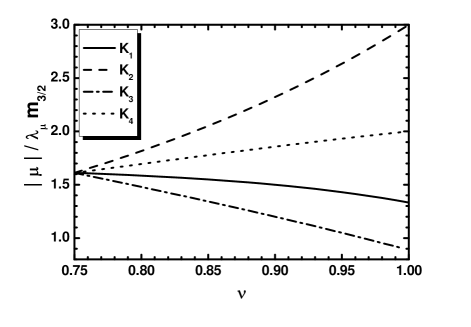
Figure 3: The ratios $|\mu|/\lambda_{\mu}m_{3/2}$ for $K=K_{1},K_{2},K_{3},$ and $K_{4}$ (solid, dashed, dot-dashed, and dotted line respectively) versus $\nu$ in the range $0.75-1$.

The magnitude of the $\mu$’s in Eq. (45) is demonstrated in Fig. 3, where we present the ratios $|\mu|/\lambda_{\mu}m_{3/2}$ for $K=K_{1}$ (solid line), $K_{2}$ (dashed line), $K_{3}$ (dot-dashed line), and $K_{4}$ (dotted line) versus $\nu$ for $3/4<\nu<1$. By coincidence all cases converge at the value $|\mu|/\lambda_{\mu}m_{3/2}\simeq 1.6$ for $\nu=3/4$. For $\lambda_{\mu}$’s of order unity, the $|\mu|$ values are a little enhanced w.r.t. $m_{3/2}$ and increase for $K=K_{2}$ and $K_{4}$ or decrease for $K=K_{1}$ and $K_{3}$ as $\nu$ increases.

IV Reheating Stage

Soon after FHI the Hubble rate $H$ becomes of the order of their masses and the IS and $z$ enter into an oscillatory phase about their minima and eventually decay via their coupling to lighter degrees of freedom. Note that ${\theta}$ remains well stabilized at zero during and after FHI and so it does not participate in the phase of dumped oscillations. Since $\langle{z}\rangle\sim m_{\rm P}$ – see Eq. (22) –, the initial energy density of its oscillations is $\rho_{z\rm I}\sim m_{z}^{2}\langle{z}\rangle^{2}$. It is comparable with the energy density of the Universe at the onset of these oscillations $\rho_{\rm t}=3m_{\rm P}^{2}H^{2}\simeq 3m_{\rm P}^{2}m_{z}^{2}$ and so we expect that $z$ will dominate the energy density of the Universe until completing its decay through its weak gravitational interactions. Actually, this is a representative case of the infamous cosmic moduli problem baerh ; moduli where reheating is induced by long-lived massive particles with mass around the weak scale.

The reheating temperature is determined by rh

$$T_{\rm rh}=\left({72/5\pi^{2}g_{\rm rh*}}\right)^{1/4}{\Gamma}_{{\delta}z}^{1/2}m_{\rm P}^{1/2},$$ (47)

where $g_{\rm rh*}\simeq 10.75-100$ counts the effective number of the relativistic degrees of freedom at $T_{\rm rh}$. Moreover, the total decay width ${\Gamma}_{{\delta}z}$ of the (canonically normalized) sgoldstino

$$\widehat{\delta z}=\langle{K^{1/2}_{ZZ^{*}}}\rangle{\delta}z~{}~{}\mbox{with}~{}~{}{\delta}z=z-\langle{z}\rangle~{}~{}\mbox{and}~{}~{}\langle{K_{ZZ^{*}}}\rangle=\langle{\omega}\rangle^{-2}$$ (48)

predominantly includes the contributions from its decay into pseudo-sgoldstinos and Higgs bosons via the kinetic terms $K_{XX^{*}}\partial_{\mu}X\partial^{\mu}X^{*}$ with $X=Z,{H_{u}}$ and ${H_{d}}$ full ; baerh ; antrh ; nsrh of the Lagrangian. In particular, we have

$${\Gamma}_{{\delta}z}\simeq{\Gamma}_{{\theta}}+{\Gamma}_{\tilde{h}},$$ (49)

where the individual decay widths are given by

$${\Gamma}_{{\theta}}\simeq\frac{\lambda_{\theta}^{2}m_{z}^{3}}{32\pi m_{\rm P}^{2}}\sqrt{1-{4m_{\theta}^{2}}/{m_{3/2}^{2}}}$$ (50a)

with $$\lambda_{\theta}=-\langle{z}\rangle/{Nm_{\rm P}}=({4\nu-3})/{\sqrt{6}\nu}$$, and

$${\Gamma}_{\tilde{h}}=\frac{3^{2\nu+1}}{2^{4\nu+1}}\lambda_{\mu}^{2}\frac{\omega^{2}}{4\pi}\frac{m_{z}^{3}}{m_{\rm P}^{2}}\nu^{-4\nu}\,.$$ (50b)

Other possible decay channels into gauge bosons through anomalies and three-body MSSM (s)particles are subdominant. On the other hand, we kinematically block the decay of $\widehat{\delta z}$ into $\widetilde{G}$’s koichi ; baerh in order to protect our setting from complications with BBN due to possible late decay of the produced $\widetilde{G}$ and problems with the abundance of the subsequently produced lightest SUSY particles. In view of Eqs. (25c) and (25a), this aim can be elegantly achieved if we set $\nu>3/4$.

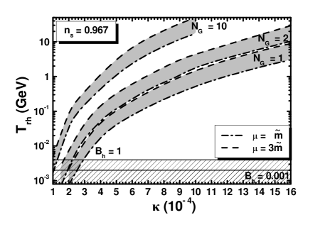
Figure 4: Allowed strips in the $\kappa-T_{\rm rh}$ plane compatible with the inflationary requirements in Sec. V for $n_{\rm s}=0.967$, and various ${\sf N}_{\rm G}$ values indicated in the graph. We take $K=K_{1}$, $\nu=7/8$, and $\mu=\widetilde{m}$ (dot-dashed lines) or $\mu=3\widetilde{m}$ (dashed lines). The BBN lower bounds on $T_{\rm rh}$ for hadronic branching ratios ${\sf B}_{\rm h}=1$ and $0.001$ are also depicted by two thin lines.

Taking $\kappa$ and $m_{z}$ values allowed by the inflationary part of our model – see Sec. VI – and selecting some specific $K$ from Eqs. (40a) – (40d), we evaluate $T_{\rm rh}$ as a function of $\kappa$ and determine the regions allowed by the BBN constraints in Eqs. (59a) and (59b) – see Sec. V below. The results of this computation are displayed in Fig. 4, where we design allowed contours in the $\kappa-T_{\rm rh}$ plane for the various ${\sf N}_{\rm G}$’s and $\nu=7/8$. This is an intermediate value in the selected margin $(3/4-1)$. The boundary curves of the allowed regions correspond to $\mu=\widetilde{m}$ or $\lambda_{\mu}=0.65$ (dot-dashed line) and $\mu=3\widetilde{m}$ or $\lambda_{\mu}=1.96$ (dashed line). The $|\mu|/\widetilde{m}-\lambda_{\mu}$ correspondence is determined via Eq. (45) for a selected $K$. Here we set $K=K_{1}$. Qualitatively similar results are obtained for an alternative $K$ choice. We see that there is an ample parameter space consistent with the BBN bounds depicted by two horizontal lines. Since the satisfaction of the inflationary requirements leads to an increase of the scale $m$ with ${\sf N}_{\rm G}$ and $m$ heavily influences $m_{z}$ and consequently $T_{\rm rh}$ – see Eq. (47) – this temperature increases with ${\sf N}_{\rm G}$. The maximal values of $T_{\rm rh}$ for the selected $\nu$ are obtained for $\mu=3\widetilde{m}$ and are estimated to be

$$T_{\rm rh}^{\max}\simeq 14~{}{\mbox{\rm GeV}},~{}33~{}{\mbox{\rm GeV}},~{}\mbox{and}~{}~{}49~{}{\mbox{\rm GeV}}$$ (51)

for ${\sf N}_{\rm G}=1,~{}2,$ and $10$ respectively. Obviously, reducing $\mu$ below $\widetilde{m}$, the parameters $\lambda_{\mu}$, ${\Gamma}_{{\delta}z}$, and so $T_{\rm rh}$ decrease too and the slice cut by the BBN bound increases. Therefore, our setting fits better with high-scale SUSY strumia and not with split strumia or natural baerh SUSY which assume $\mu\ll\widetilde{m}$.

V Observational Requirements

Our set-up must satisfy a number of observational requirements specified below.

The number of e-foldings that the pivot scale $k_{\star}=0.05/{\rm Mpc}$ undergoes during FHI must be adequately large for the resolution of the horizon and flatness problems of standard Big Bang cosmology. Assuming that FHI is followed, in turn, by a decaying-particle, radiation and matter dominated era, we can derive the relevant condition hinova ; plin :

$${N_{\rm I\star}}=\int_{\sigma_{\rm f}}^{\sigma_{\star}}\frac{d\sigma}{m^{2}_{\rm P}}\>\frac{V_{\rm I}}{V^{\prime}_{\rm I}}\simeq 19.4+{2\over 3}\ln{V^{1/4}_{\rm I0}\over{1~{}{\rm GeV}}}+{1\over 3}\ln{T_{\rm rh}\over{1~{}{\rm GeV}}},$$ (52)

where the prime denotes derivation w.r.t. $\sigma$, $\sigma_{\star}$ is the value of $\sigma$ when $k_{\star}$ crosses outside the inflationary horizon, and $\sigma_{\rm f}$ is the value of $\sigma$ at the end of FHI. The latter coincides with either the critical point $\sigma_{\rm c}=\sqrt{2}|S_{\rm c}|$ – see Eq. (33) –, or the value of $\sigma$ for which one of the slow-roll parameters review

$$\epsilon={m^{2}_{\rm P}}\left({V^{\prime}_{\rm I}}/\sqrt{2}{V_{\rm I}}\right)^{2}~{}~{}\mbox{or}~{}~{}\eta=m^{2}_{\rm P}~{}{V^{\prime\prime}_{\rm I}}/{V_{\rm I}}$$ (53)

exceeds unity in absolute value. For $\lambda\sim 10^{-12}$ as required by the cosmic coincidence problem – see below – we obtain $\langle{\sigma}\rangle\simeq 0$ which does not disturb the inflationary dynamics since $\langle{\sigma}\rangle\ll\sigma_{\rm c}$.

The amplitude $A_{\rm s}$ of the power spectrum of the curvature perturbation generated by $\sigma$ during FHI and calculated at $k_{\star}$ as a function of $\sigma_{\star}$ must be consistent with the data plcp , i.e.,

$$\sqrt{A_{\rm s}}=\frac{1}{2\sqrt{3}\,\pi m^{3}_{\rm P}}\;\left.\frac{V_{\rm I}^{3/2}(\sigma_{\star})}{|V^{\prime}_{\rm I}(\sigma_{\star})|}\right.\simeq\>4.588\times 10^{-5}.$$ (54)

The observed curvature perturbation is generated wholly by $\sigma$ since the other scalars are adequately massive during FHI – see Sec. II.3.1.

The scalar spectral index $n_{\rm s}$, its running $\alpha_{\rm s}$, and the scalar-to-tensor ratio $r$ must be in agreement with the fitting of the Planck TT, TE, EE+lowE+lensing, BICEP/Keck Array (BK18), and BAO data plin ; gws with the $\Lambda$CDM$+r$ model which approximately requires that, at 95$\%$ confidence level (c.l.),

$$n_{\rm s}=0.967\pm 0.0074\>\>\>\mbox{and}\>\>\>r\leq 0.032,$$ (55)

with $|\alpha_{\rm s}|\ll 0.01$. These observables are calculated employing the standard formulas

$$n_{\rm s}=1-6\epsilon_{\star}\ +\ 2\eta_{\star},$$ (56a)

$$\alpha_{\rm s}={2}\left(4\eta_{\star}^{2}-(n_{\rm s}-1)^{2}\right)/3-2\xi_{\star},~{}\mbox{and}~{}~{}r=16\epsilon_{\star},$$ (56b)

where $\xi\simeq m_{\rm P}^{4}~{}V^{\prime}_{\rm I}V^{\prime\prime\prime}_{\rm I}/V^{2}_{\rm I}$ and all the variables with the subscript $\star$ are evaluated at $\sigma=\sigma_{\star}$.

The dimensionless tension ${G\mu_{\rm cs}}$ of the $B-L$ CSs produced at the end of FHI in the case $\mathbb{G}=\mathbb{G}_{B-L}$ is mark

$${G\mu_{\rm cs}}\simeq\frac{1}{2}\left(\frac{M}{m_{\rm P}}\right)^{2}{\epsilon_{\rm cs}}({r_{\rm cs}})~{}~{}\mbox{with}~{}~{}{\epsilon_{\rm cs}}({r_{\rm cs}})=\frac{2.4}{\ln(2/{r_{\rm cs}})}\cdot$$ (57)

Here $G=1/8\pi m_{\rm P}^{2}$ is the Newton gravitational constant and ${r_{\rm cs}}=\kappa^{2}/2g^{2}\leq 10^{-2}$ with $g\simeq 0.7$ being the gauge coupling constant at a scale close to $M$. ${G\mu_{\rm cs}}$ is restricted by the level of the CS contribution to the observed anisotropies of CMB radiation reported by Planck plcs0 as follows:

$${G\mu_{\rm cs}}\lesssim 2.4\times 10^{-7}~{}~{}\mbox{at 95$\%$ c.l.}$$ (58a)

On the other hand, the primordial CS loops and segments connecting monopole pairs decay by emitting stochastic gravitational radiation which is measured by the pulsar timing array experiments nano ; pta . If the CS network is stable, the recent observations require nano1

$${G\mu_{\rm cs}}\lesssim 2\times 10^{-10}~{}~{}\mbox{at 95$\%$ c.l.}$$ (58b)

However, if the CSs are metastable, due to the embedding of $$\mathbb{G}_{B-L} \mathbb{G}_{\rm GUT}$$ into a larger group whose breaking leads to monopoles which can break the CSs, the interpretation nano1 of the recent observations nano ; pta dictates

$$10^{-8}\lesssim{G\mu_{\rm cs}}\lesssim 2\times 10^{-7}~{}~{}\mbox{for}~{}~{}8.2\gtrsim\sqrt{{r_{\rm ms}}}\gtrsim 7.9$$ (58c)

at $2\sigma$ where the upper bound originates from Ref. ligo and is valid for a standard cosmological evolution and CSs produced after inflation. Here ${r_{\rm ms}}$ is the ratio of the monopole mass squared to $\mu_{\rm cs}$. Since we do not specify further this possibility in our work, the last restriction does not impact on our parameters.

Consistency between theoretical and observational values of light element abundances predicted by BBN imposes a lower bound on $T_{\rm rh}$, which depends on the mass of the decaying particle $z$ and the hadronic branching ratio ${\sf B}_{\rm h}$. Namely, for large $m_{z}\sim 10^{5}~{}{\mbox{\rm GeV}}$, the most up-to-date analysis of Ref. nsref entails

$$T_{\rm rh}\geq 4.1~{}{\mbox{\rm MeV}}~{}~{}\mbox{for}~{}~{}{\sf B}_{\rm h}=1$$ (59a)

and $$T_{\rm rh}\geq 2.1~{}{\mbox{\rm MeV}}~{}~{}\mbox{for}~{}~{}{\sf B}_{\rm h}=10^{-3}.$$ (59b)

The BBN bound is mildly softened for larger $m_{z}$ values. Moreover, the possible production of $\widetilde{G}$ from the $z$ decay is mostly problematic baerh since it may lead to overproduction of the LSP (i.e., the lightest SUSY particle), whose non-thermally produced abundance from the $\widetilde{G}$ decay can drastically overshadow its thermally-produced one. As a consequence, the LSP abundance can easily violate the observational upper bound plcp from CDM considerations. This is the moduli-induced koichi LSP overproduction problem via the $\widetilde{G}$ decay baerh . To avoid this complication, we kinematically forbid the decay of $z$ into $\widetilde{G}$ selecting $\nu>3/4$ which ensures that $m_{z}<2m_{3/2}$ – see Eq. (25c).

We identify $\langle{V_{\rm F}}\rangle$ in Eq. (23) with the DE energy density, i.e.,

$$\langle{V_{\rm F}}\rangle=\Omega_{\Lambda}\rho_{\rm c0}=7.2\times 10^{-121}m_{\rm P}^{4},$$ (60)

where $\Omega_{\Lambda}=0.6889$ and $\rho_{\rm c0}=2.4\times 10^{-120}h^{2}m_{\rm P}^{4}$ with $h=0.6732$ plcp are the density parameter of DE and the current critical energy density of the Universe respectively. By virtue of Eq. (23), we see that Eq. (60) can be satisfied for $\lambda\sim m/m_{\rm P}$. Explicit values are given for the cases in Table 1.

Scenarios with large $\widetilde{m}$, although not directly accessible at the LHC, can be probed via the measured value of the Higgs boson mass. Within high-scale SUSY, updated analysis requires lhc ; strumia

$$3\times 10^{3}\lesssim\widetilde{m}/{\mbox{\rm GeV}}\lesssim 3\times 10^{11},$$ (61)

for degenerate sparticle spectrum, $\mu$ and $\tan\beta$ in the ranges $\widetilde{m}/3\leq\mu\leq 3\widetilde{m}$ and $1\leq\tan\beta\leq 50$, and varying the stop mixing.

VI Results

As deduced from Secs. II.1.1 – II.1.3 and III, our model depends on the parameters

$${\sf N}_{\rm G},~{}\kappa,~{}M,~{}m,~{}\lambda,~{}\nu,~{}k,~{}~{}\mbox{and}~{}~{}\lambda_{\mu}$$

(recall that $N$ is related to $\nu$ via Eq. (7)). Let us initially clarify that $\lambda$ can be fixed at a rather low value as explained below Eq. (60) and does not influence the rest of our results. Moreover, $k$ affects $m_{\theta}$ and $m_{\rm I\theta}$ via Eqs. (25c) and (31a) and helps us to avoid massless modes. We take $k=0.1$ throughout our investigation.

As shown in Ref. mfhi , the confrontation of FHI with data for any fixed ${\sf N}_{\rm G}$ requires a specific adjustment between $\kappa$ or $M$ and the ${\rm a}_{S}$ which is given in Eq. (38d) as a function of $m$, $\nu$, $\kappa$, and $M$ – see Eq. (30). Obviously a specific ${\rm a}_{S}$ value can be obtained by several choices of the initial parameters $\nu$ and $m$. These parameters influence also the requirement in Eq. (52) via $T_{\rm rh}$, which is given in Eq. (47). However, to avoid redundant solutions we first explore our results for the IS in terms of the variables $\kappa,M,$ and ${\rm a}_{S}$ in Sec. VI.1 taking a representative $T_{\rm rh}$ value, e.g., $T_{\rm rh}\simeq 1~{}{\mbox{\rm GeV}}$. Variation of $T_{\rm rh}$ over one or two orders of magnitude does not affect our findings in any essential way. Therefore, we do not impose in Sec. VI.1 the constraints from the BBN in Eqs. (59a) and (59b). In Sec. VI.2, we then interconnect these results with the HS parameters $\nu$ and $m$.

VI.1 Inflation Analysis

Enforcing the constraints in Eqs. (52) and (54) we can find $M$ and $\sigma_{\star}$, for any given ${\sf N}_{\rm G}$, as functions of our free parameters $\kappa$ and ${\rm a}_{S}$. Let us clarify here that for ${\sf N}_{\rm G}=1$ the parameter space is identical with the one explored in Ref. mfhi , where the HS is not specified. As explained there – see also Ref. kaihi – observationally acceptable values of $n_{\rm s}$ can be achieved by implementing hilltop FHI. This type of FHI requires a non-monotonic $V_{\rm I}$ with $\sigma$ rolling from its value $\sigma_{\rm max}$ at which the maximum of $V_{\rm I}$ lies down to smaller values. As for any model of hilltop inflation, $V_{\rm I}^{\prime}$ and therefore $\epsilon$ in Eq. (53) and $r$ in Eq. (56b) decrease sharply as $N_{\rm I\star}$ increases – see Eq. (52) –, whereas $V_{\rm I}^{\prime\prime}$ (or $\eta$) becomes adequately negative, thereby lowering $n_{\rm s}$ within its range in Eq. (55).

These qualitative features are verified by the approximate computation of the quantities in Eq. (53) for $\sigma<\sigma_{\rm max}$ which are found to be

$$\epsilon\simeq m_{\rm P}^{2}\left(C^{\prime}_{\rm RC}+C^{\prime}_{\rm SSB}\right)^{2}/2~{}~{}\mbox{and}~{}~{}\eta\simeq m_{\rm P}^{2}C^{\prime\prime}_{\rm RC},$$ (62)

where the derivatives of the various contributions read

$$C^{\prime}_{\rm SSB} \simeq-{\rm a}_{S}/\sqrt{2V_{\rm I0}},$$ (63a)

$$C^{\prime}_{\rm RC} \simeq\frac{{\sf N}_{\rm G}\kappa^{2}x}{32M\pi^{2}}\left(4\tanh^{-1}\left({2}/{x^{2}}\right)+x^{2}\ln(1-4/x^{4})\right),$$ (63b)

$$C^{\prime\prime}_{\rm RC} \simeq\frac{{\sf N}_{\rm G}\kappa^{2}}{32M^{2}\pi^{2}}\left(4\tanh^{-1}\left({2}/{x^{2}}\right)+3x^{2}\ln(1-4/x^{4})\right).$$ (63c)

The required behavior of $V_{\rm I}$ in Eq. (37) can be attained, for given ${\sf N}_{\rm G}$, thanks to the similar magnitudes and the opposite signs of the terms $C^{\prime}_{\rm RC}$ and $C^{\prime}_{\rm SSB}$ in Eqs. (63a) and (63b) which we can obtain for carefully selecting $\kappa$ and ${\rm a}_{S}$. Apparently, we have $C^{\prime}_{\rm SSB}<0$ and $C^{\prime}_{\rm RC}>0$ for $\sigma_{\star}<\sigma_{\rm max}$ since $|4\tanh^{-1}\left({2}/{x^{2}}\right)|>|x^{2}\ln(1-4/x^{4})|$. On the contrary, $C^{\prime\prime}_{\rm RC}<0$, since the negative contribution $3x^{2}\ln(1-4/x^{4})$ dominates over the first positive one, and so we obtain $\eta<0$ giving rise to acceptably low $n_{\rm s}$ values.

Figure 5: $V_{\rm I}$ as a function of $\sigma$ in units of $M$ for the parameters given in column B of Table 1. The values $\sigma_{\star}$, $\sigma_{\rm f}$, $\sigma_{\rm max}$, and $\sigma_{\rm min}$ of $\sigma$ are also depicted.

We can roughly determine $\sigma_{\rm max}$ by expanding $C^{\prime}_{\rm RC}$ for large $\sigma$ and equating the result with $C^{\prime}_{\rm SSB}$. We obtain

$$\frac{{\sf N}_{\rm G}\kappa^{2}}{8\pi^{2}\sigma_{\rm max}}=\frac{{\rm a}_{S}}{\sqrt{2}\kappa M^{2}}~{}\Rightarrow~{}\sigma_{\rm max}\simeq\frac{\kappa^{3}M^{2}{\sf N}_{\rm G}}{4\sqrt{2}\pi^{2}{\rm a}_{S}}.$$ (64)

Needless to say, $V_{\rm I}$ turns out to be bounded from below for large $\sigma$’s since in this regime $C_{\rm SUGRA}$ starts dominating over $C_{\rm RC}$ generating thereby a (${\sf N}_{\rm G}$-independent) minimum at about

$$\sigma_{\rm min}\simeq\left(\frac{{\rm a}_{S}m_{\rm P}^{4}}{\sqrt{2}c_{4\nu}\kappa M^{2}}\right)^{1/3}\cdot$$ (65)

For $\sigma>\sigma_{\rm min}$, $V_{\rm I}$ becomes a monotonically increasing function of $\sigma$ and so the boundedness of $V_{\rm I}$ is assured.

From our numerical computation we observe that, for constant ${\sf N}_{\rm G},\kappa$, and ${\rm a}_{S}$, the lower the value for $n_{\rm s}$ we wish to attain, the closer we must set $\sigma_{\star}$ to $\sigma_{\rm max}$. Given that $\sigma_{\rm max}$ turns out to be comparable to $\sigma_{\rm c}$ and the hierarchy $\sigma_{\rm c}<\sigma_{\star}<\sigma_{\rm max}$ has to hold, we see that we need two types of mild tunings in order to obtain successful FHI. To quantify the amount of these tunings, we define the quantities

$$\Delta_{\rm c\star}={\sigma_{\star}-\sigma_{\rm c}\over\sigma_{\rm c}}~{}~{}\mbox{and}~{}~{}\Delta_{\rm max*}={\sigma_{\rm max}-\sigma_{\star}\over\sigma_{\rm max}}\,.$$ (66)

The naturalness of the hilltop FHI increases with $\Delta_{\rm c\star}$ and $\Delta_{\rm max*}$. To get an impression of the amount of these tunings and their dependence on the parameters of the model, we display in Table 1 the resulting $\Delta_{\rm c\star}$ and $\Delta_{\rm max*}$ together with $M$, ${\rm a}_{S}$, $\alpha_{\rm s}$, and $r$ for $\kappa=0.0005$ and $n_{\rm s}$ fixed to its central value in Eq. (55). In all cases, we obtain $N_{\rm I\star}\simeq 40.5$ from Eq. (52). We notice that $\Delta_{\rm max*}>\Delta_{\rm c\star}$ and that their values may be up to $10\%$ increasing with ${\sf N}_{\rm G}$ (and ${\rm a}_{S}$). Recall that in Ref. mfhi it is shown that $\Delta_{\rm c\star}$ and $\Delta_{\rm max*}$ increase with $\kappa$ (and $M$). From the observables listed in Table 1 we also infer that $|\alpha_{\rm s}|$ turns out to be of order $10^{-4}$, whereas $r$ is extremely tiny, of order $10^{-11}$, and therefore far outside the reach of the forthcoming experiments devoted to detect primordial gravity waves. For the preferred $n_{\rm s}$ values, we observe that $r$ and $|\alpha_{\rm s}|$ increase with ${\rm a}_{S}$.

The structure of $V_{\rm I}$ described above is visualized in Fig. 5, where we display a typical variation of $V_{\rm I}$ as a function of $\sigma/M$ for the values of the parameters shown in column B of Table 1. The maximum of $V_{\rm I}$ is located at $\sigma_{\rm max}/M=1.52\,\{1.38\}$, whereas its minimum lies at $\sigma_{\rm min}/M=29.1\,\{29.5\}$ – the values obtained via the approximate Eqs. (64) and (65) are indicated in curly brackets. The values of $\sigma_{\star}/M\simeq 1.4637$ and $\sigma_{\rm f}/M\simeq 1.41421$ are also depicted together with $\sigma_{\rm max}/M$ in the subplot of this figure. We remark that the key $\sigma$ values for the realization of FHI are squeezed very close to one another and so their accurate determination is essential for obtaining reliable predictions from Eqs. (56a) and (56b). Moreover, $N_{\rm I\star}$ in Eq. (52) can only be found numerically taking all the possible contributions to $V_{\rm I}^{\prime}$ from Eqs. (63a) and (63b) and thus $\sigma_{\star}$ can not be expressed analytically in terms of $N_{\rm I\star}$. For these reasons, the results presented in the following are exclusively based on our numerical analysis.

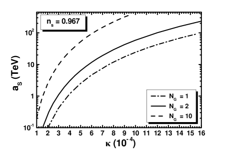
Figure 6: Values of ${\rm a}_{S}$ allowed by Eqs. (52) and (54) versus $\kappa$ for various ${\sf N}_{\rm G}$’s and fixed $n_{\rm s}=0.967$.

We first display in Fig. 6 the contours which are allowed by Eqs. (52) and (54) in the $\kappa-{\rm a}_{S}$ plane taking $n_{\rm s}=0.967$ and ${\sf N}_{\rm G}=1$ (dot-dashed line), ${\sf N}_{\rm G}=2$ (solid line), and ${\sf N}_{\rm G}=10$ (dashed line). The various lines terminate at $\kappa$ values close to $10^{-3}$ beyond which no observationally acceptable inflationary solutions are possible. We do not depict the very narrow strip obtained for each ${\sf N}_{\rm G}$ by varying $n_{\rm s}$ in its allowed range in Eq. (55), since the obtained boundaries are almost indistinguishable. From the plotted curves we notice that the required ${\rm a}_{S}$’s increase with ${\sf N}_{\rm G}$.

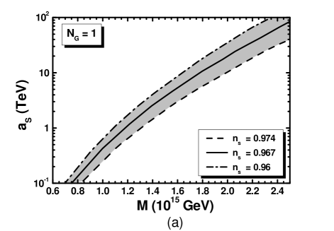
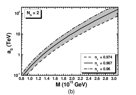
Figure 7: Regions (shaded) allowed by Eqs. (52), (54), and (55) in the $M-{\rm a}_{S}$ plane for ${\sf N}_{\rm G}=1$ (a), ${\sf N}_{\rm G}=2$ (b) and ${\sf N}_{\rm G}=10$ (c). The conventions adopted for the various lines are also shown.

Working in the same direction, we delineate in Fig. 7 the regions in the $M-{\rm a}_{S}$ plane allowed by Eqs. (52), (54), and (55) for the considered $\mathbb{G}$’s. In particular, we use ${\sf N}_{\rm G}=1,2,$ and $10$ in subfigures (a), (b), and (c) respectively. The boundaries of the allowed areas in Fig. 7 are determined by the dashed [dot-dashed] lines corresponding to the upper [lower] bound on $n_{\rm s}$ in Eq. (55). We also display by solid lines the allowed contours for $n_{\rm s}=0.967$. We observe that the maximal allowed $M$’s increase with ${\sf N}_{\rm G}$. The maximal $r$’s are encountered in the upper right end of the dashed lines, which correspond to $n_{\rm s}=0.974$, with the maximal value being $r=6.2\times 10^{-10}$ for ${\sf N}_{\rm G}=10$. On the other hand, the maximal $|\alpha_{\rm s}|$’s are achieved along the dot-dashed lines and the minimal value of $\alpha_{\rm s}$ is $-3.2\times 10^{-4}$ for ${\sf N}_{\rm G}=10$ too. Summarizing our findings from Fig. 7 for the central $n_{\rm s}$ value in Eq. (55) and ${\sf N}_{\rm G}=1,2,$ and $10$ respectively we end up with the following ranges:

$$0.07\lesssim{M/10^{15}~{}{\rm GeV}}\lesssim 2.56~{}~{}\mbox{and}~{}~{}0.1\lesssim{{\rm a}_{S}/{\mbox{\rm TeV}}}\lesssim 100,$$ (67a)

$$0.82\lesssim{M/10^{15}~{}{\rm GeV}}\lesssim 3.7~{}~{}\mbox{and}~{}~{}0.09\lesssim{{\rm a}_{S}/{\mbox{\rm TeV}}}\lesssim 234,$$ (67b)

$$1.22\lesssim{M/10^{15}~{}{\rm GeV}}\lesssim 4.77~{}~{}\mbox{and}~{}~{}0.2\lesssim{{\rm a}_{S}/{\mbox{\rm TeV}}}\lesssim 460.$$ (67c)

Within these margins, $\Delta_{\rm c\star}$ ranges between $0.5\%$ and $20\%$ and $\Delta_{\rm max*}$ between $0.4\%$ and $12\%$. The lower bounds of these inequalities are expected to be displaced to slightly larger values due to the post-inflationary requirements in Eqs. (59a) and (59b) which are not considered here for the shake of generality. Recall that precise incorporation of these constraints requires the adoption of a specific $K$ from Eqs. (40a) – (40d) and corresponding $\mu/\widetilde{m}$ relation from Eq. (45).

In the case $\mathbb{G}=\mathbb{G}_{B-L}$, CSs may be produced after FHI with ${G\mu_{\rm cs}}=(6.5-89)\times 10^{-9}$ for the parameters in Eq. (67a). Therefore, the corresponding parameter space is totally allowed by Eq. (58a) but completely excluded by Eq. (58b), if the CSs are stable. If these CSs are metastable, the explanation kainano of the recent data nano ; pta on stochastic gravity waves is possible for $M\gtrsim 9\times 10^{14}~{}{\mbox{\rm GeV}}$ in Eq. (67a) where Eq. (58c) is fulfilled. No similar restrictions exist if $\mathbb{G}=\mathbb{G}_{\rm LR}$ or $\mathbb{G}_{\rm 5_{X}}$, which do not lead to the production of any cosmic defect. On the other hand, the unification of gauge coupling constants within MSSM close to $M_{\rm GUT}=2.86\times 10^{16}~{}{\mbox{\rm GeV}}$ remains intact if $\mathbb{G}=\mathbb{G}_{B-L}$ despite the fact that $M\ll M_{\rm GUT}$ for $M$ given in Eq. (67a). Indeed, the gauge boson associated with the $U(1)_{B-L}$ breaking is neutral under $\mathbb{G}_{\rm SM}$ and so it does not contribute to the relevant renormalization group running. If $\mathbb{G}=\mathbb{G}_{\rm LR}$ or $\mathbb{G}_{\rm 5_{X}}$ we may invoke threshold corrections or additional matter supermultiples to restore the gauge coupling unification – for $\mathbb{G}=\mathbb{G}_{\rm 5_{X}}$ see Ref. flipnew .

VI.2 Link to the MSSM

The inclusion of the HS in our numerical computation assists us to gain information about the mass scale of the SUSY particles through the determination of $\widetilde{m}\sim m_{3/2}$ – see Eq. (46). Indeed, ${\rm a}_{S}$, which is already restricted as a function of $\kappa$ or $M$ for given ${\sf N}_{\rm G}$ in Figs. 6 and 7, can be correlated to $m$ via Eq. (38d). Taking into account Eq. (30) and the fact that $\langle{z}\rangle_{\rm I}/m_{\rm P}\sim 10^{-3}$ – see Table 1 – we can solve analytically and very accurately Eq. (38d) w.r.t. $m$. We find

$$m\simeq\left(\frac{{\rm a}_{S}}{2^{1+\nu}(2-\nu)}\right)^{(2-\nu)/2}\left(\frac{3H_{\rm I}^{2}}{(1-\nu)\nu^{2}}\right)^{\nu/4}.$$ (68)

Let us clarify here that in our numerical computation we use an iterative process, which though converges quickly, in order to extract consistently $m$ as a function of $\kappa$ and $M$. This is because the determination of the latter parameters via the conditions in Eqs. (52) and (54) requires the introduction of a trial $m$ value which allows us to use as input the form of $V_{\rm I}$ in Eq. (37). Thanks to the aforementioned smallness of $\langle{z}\rangle_{\rm I}$ in Eq. (38d), $m$ turns out to be two to three orders of magnitude larger than ${\rm a}_{S}$, suggesting that $\widetilde{m}$ lies clearly at the PeV scale via Eqs. (46) and (25a). In fact, taking advantage of the resulting $m$ for fixed $\nu$ in Eq. (68), we can compute $m_{3/2}$ from Eq. (25a), and $m_{z}$ and $m_{\theta}$ from Eq. (25c). All these masses turn out to be of the same order of magnitude – see Table 1. Then $\widetilde{m}$ and $T_{\rm rh}$ can be also estimated from Eqs. (46) and (47) for a specific $K$ from Eqs. (40a) – (40d). The magnitude of $\widetilde{m}$ and the necessity for $\mu\sim\widetilde{m}$, established in Sec. IV, hints towards the high-scale MSSM.

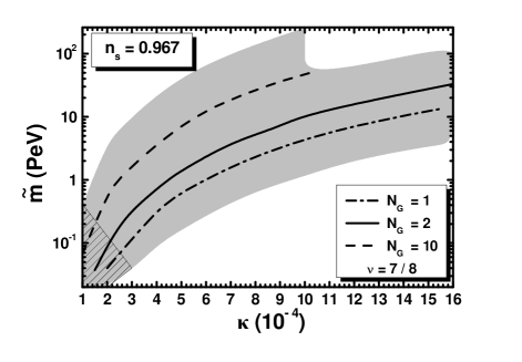
Figure 8: Region in the $\kappa-\widetilde{m}$ plane allowed by Eqs. (52) and (54)for $K=K_{1}$, $\mu=\widetilde{m}$, $n_{\rm s}=0.967$, and $1\leq{\sf N}_{\rm G}\leq 10$, $3/4<\nu<1$. The allowed contours for $\nu=7/8$ are also depicted. Hatched is the region excluded by BBN for ${\sf B}_{\rm h}=0.001$.

To highlight numerically our expectations, we take $K=K_{1}$ and fix initially $\nu=7/8$, which is a representative value. The predicted $\widetilde{m}$ as a function of $\kappa$ is depicted in Fig. 8 for the three ${\sf N}_{\rm G}$’s considered in our work. We use the same type of lines as in Fig. 6. Assuming also that $\mu=\widetilde{m}$ we can determine the segments of these lines that can be excluded by the BBN bound in Eq. (59b). In all, we find that $\widetilde{m}$ turns out to be confined in the ranges

$$0.34\lesssim\widetilde{m}/{\mbox{\rm PeV}}\lesssim 13.6~{}~{}\mbox{for}~{}~{}{\sf N}_{\rm G}=1,$$ (69a)

$$0.21\lesssim\widetilde{m}/{\mbox{\rm PeV}}\lesssim 32.9~{}~{}\mbox{for}~{}~{}{\sf N}_{\rm G}=2,$$ (69b)

$$0.58\lesssim\widetilde{m}/{\mbox{\rm PeV}}\lesssim 46.8~{}~{}\mbox{for}~{}~{}{\sf N}_{\rm G}=10.$$ (69c)

Allowing $\nu$ and $\mu$ to vary within their possible respective margins $(0.75-1)$ and $(1-3)\widetilde{m}$, we obtain the gray shaded region in Fig. 8. We present an overall region for the three possible ${\sf N}_{\rm G}$’s, since the separate ones overlap each other. Obviously the lower boundary curve of the displayed region is obtained for ${\sf N}_{\rm G}=1$ and $\nu\simeq 0.751$, whereas the upper one corresponds to ${\sf N}_{\rm G}=10$ and $\nu\simeq 0.99$. The hatched region is ruled out by Eq. (59b). All in all, we obtain the predictions

$$1.2\lesssim{\rm a}_{S}/{\mbox{\rm TeV}}\lesssim 460~{}~{}\mbox{and}~{}~{}0.09\lesssim\widetilde{m}/{\mbox{\rm PeV}}\lesssim 253$$ (70)

and $T_{\rm rh}^{\max}\simeq 71~{}{\mbox{\rm GeV}},139~{}{\mbox{\rm GeV}},$ and $163~{}{\mbox{\rm GeV}}$ for ${\sf N}_{\rm G}=1,2,$ and $10$ respectively attained for $\mu=3\widetilde{m}$ and $\nu\simeq 0.99$. The derived allowed margin of $\widetilde{m}$, which is included in Eq. (61), and the employed $\mu$ values render our proposal compatible with the mass of the Higgs boson discovered in LHC lhc if we adopt as a low energy effective theory the high-scale version of MSSM strumia .

VII Conclusions

We considered the realization of FHI in the context of an extended model based on the superpotential and Kähler potential in Eqs. (1) and (5), which are consistent with an approximate $R$ symmetry. The minimization of the SUGRA scalar potential at the present vacuum constrains the curvature of the internal space of the goldstino superfield and provides a tunable energy density which may be interpreted as the DE without the need of an unnaturally small coupling constant. On the other hand, this same potential causes a displacement of the sgoldstino to values much smaller than $m_{\rm P}$ during FHI. Combining this fact with minimal kinetic terms for the inflaton, the $\eta$ problem is resolved allowing hilltop FHI. The slope of the inflationary path is generated by the RCs and a tadpole term with a minus sign and values which increase with the dimensionality of the representation of the relevant Higgs superfields. Embedding $\mathbb{G}_{B-L}$ into a larger gauge group $\mathbb{G}_{\rm GUT}$ which predicts the production of monopoles prior to FHI that can eventually break the CSs allows the attribution of the observed data on the gravitational waves to the decay of metastable $B-L$ CSs.

We also discussed the generation of the $\mu$ term of MSSM following the Giudice-Masiero mechanism and restricted further the curvature of the goldstino internal space so that phenomenologically dangerous production of $\widetilde{G}$ may be avoided. This same term assists in the decay of the sgoldstino, which normally dominates the energy density of the Universe, at a reheat temperature which can be as high as $163~{}{\mbox{\rm GeV}}$ provided that the $\mu$ parameter is of the order of the $\widetilde{G}$ mass, i.e., of order PeV. Linking the inflationary sector to a degenerate MSSM mass scale $\widetilde{m}$ we found that $\widetilde{m}$ lies in a range consistent with the Higgs boson mass measured at LHC within high-scale SUSY.

The long-lasting matter domination obtained in our model because of the sgoldstino oscillations after the end of FHI leads wells to a suppression at relatively large frequencies ($f>0.1~{}{\rm Hz}$) of the spectrum of the gravitational waves from the decay of the metastable CSs. This effect may be beneficial for spectra based on ${G\mu_{\rm cs}}$ values which violate the upper bound of Eq. (58c) from the results of Ref. ligo . Since we do not achieve such ${G\mu_{\rm cs}}$ values here we do not analyze further this implication of our scenario. On the other hand, the low reheat temperature encountered in our proposal makes difficult the achievement of baryogenesis. However, there are currently attempts bau based on the idea of cold electroweak baryogenesis cbau which may overcome this problem. It is also not clear which particle could play the role of CDM in a high-scale SUSY regime. Let us just mention that a thorough investigation is needed including the precise solution of the relevant Bolzmann equations as in Ref. rh in order to assess if the abundance of the lightest SUSY particle can be confined within the observational limits in this low-reheating scenario.

Appendix A SUGRA CORRECTIONS TO THE INFLATIONARY POTENTIAL of FHI

As shown in Sec. II.3.2, the presence of $W_{\rm H}$ and $K_{\rm H}$ in Eqs. (2b) and (6b) respectively transmit (potentially important) corrections to the inflationary potential. We present here, for the first time to the best of our knowledge, these corrections without specify the form of these functions. The corrections from the IS are also taken into account.

In particular, we consider the following superpotential and Kähler potential resulting from the ones in Eqs. (1) and (5) by setting $\Phi$ and $\bar{\Phi}$ to zero:

$$W=W_{\rm I}(S)+W_{\rm H}(Z)~{}~{}\mbox{and}~{}~{}K=K_{\rm I}(S)+K_{\rm H}(Z),$$ (71)

where $W_{\rm I}$ and $K_{\rm I}$ are given by

$$W_{\rm I}=-\hat{\kappa}M^{2}S~{}~{}\mbox{and}~{}~{}K_{\rm I}=K_{\rm I}(|S|^{2})$$ (72)

(cf. Eqs. (2a) and (6a)). We also assume that $K_{\rm I}$ can be reliably expanded in powers of $|S|/m_{\rm P}$ as follows:

$$K_{\rm I}\simeq|S|^{2}+\frac{k_{4}}{4}\frac{|S|^{4}}{m_{\rm P}^{2}}+\frac{k_{6}}{9}\frac{|S|^{6}}{m_{\rm P}^{3}}+\cdots.$$ (73)

Under these circumstances, the inverse Kähler metric reads

$$K^{SS^{*}}_{\rm I}\simeq 1-k_{4}{|S|^{2}}{m_{\rm P}^{2}}+(k_{4}^{2}-k_{6}){|S|^{4}}/{m_{\rm P}^{4}}+\cdots$$ (74a)

and the exponential prefactor of $$V_{\rm F}$$ in Eq. (9) is well approximated by

$$e^{K_{\rm I}/m_{\rm P}^{2}}\simeq 1+\frac{|S|^{2}}{m_{\rm P}^{2}}+\frac{1+2k_{4}}{2}\frac{|S|^{4}}{m_{\rm P}^{4}}+\cdots.$$ (74b)

Taking into account the two last expressions and expanding $V_{\rm F}$ in Eq. (9) with $W$ and $K$ from Eq. (71) up to the forth power in $|S|/m_{\rm P}$, we obtain the quite generic formula below

$$V_{\rm F} \simeq v_{0}+m_{\rm I3/2}^{2}|S|^{2}+\left(v_{1}S^{*}+{\rm c.c}\right)+v_{2}{|S|^{2}}/{m_{\rm P}^{2}}$$

$$+\left(v_{3}S^{*}+{\rm c.c}\right){|S|^{2}}/{m_{\rm P}^{2}}+v_{4}{|S|^{4}}/{m_{\rm P}^{4}}+\cdots,$$ (75)

where the various $v$’s are found to be

$$v_{0} =\kappa^{2}M^{4},$$ (76a)

$$v_{1} =\kappa M^{2}m_{\rm I3/2}\left\langle{2-K^{ZZ^{*}}_{\rm H}\partial_{Z}G_{\rm H}}\right\rangle_{\rm I},$$ (76b)

$$v_{2} =\kappa^{2}M^{4}\left\langle{K^{ZZ^{*}}_{\rm H}|\partial_{Z}K_{\rm H}|^{2}/m_{\rm P}^{2}-k_{4}}\right\rangle_{\rm I},$$ (76c)

$$v_{3} =\kappa M^{2}m_{\rm I3/2}\left\langle{(1+k_{4}/2)-K^{ZZ^{*}}_{\rm H}\partial_{Z}G_{\rm H}}\right\rangle_{\rm I},$$ (76d)

$$v_{4} =\kappa^{2}M^{4}\Big{(}1/2+k_{4}(4k_{4}-7)/4-k_{6}$$

$$\left.+\left\langle{K^{ZZ^{*}}_{\rm H}|\partial_{Z}K_{\rm H}|^{2}/m_{\rm P}^{2}}\right\rangle_{\rm I}\right).$$ (76e)

Here $\kappa$ is the rescaled coupling constant $\hat{\kappa}$ after absorbing the relevant prefactor $e^{\left\langle{K_{\rm H}}\right\rangle_{\rm I}/2m_{\rm P}}$ in Eq. (9) and we used the definition of the $\widetilde{G}$ mass

$$m_{\rm I3/2}=\left\langle{e^{K_{\rm H}/2m_{\rm P}^{2}}W_{\rm H}/m_{\rm P}^{2}}\right\rangle_{\rm I},$$

and the Kähler invariant function, see, e.g., Ref. gref ,

$$G_{\rm H}=K_{\rm H}/m_{\rm P}^{2}+\ln|W_{\rm H}/m_{\rm P}^{3}|^{2}.$$ (77)

From these results we see that $v_{2}$ and $v_{4}$ generically receive contributions from both the IS and HS, whereas $v_{1}$ and $v_{3}$ exclusively from the HS – cf. Refs. pana ; kelar . Specifically, from Eq. (76c), we can recover the miraculous cancellation occurring within minimal FHI mfhi ; buchbl , where the HS is ignored and $k_{4}=k_{6}=0$ in Eq. (73). Switching on $K_{\rm H}$ and noticing that

$$k_{4}=\partial^{2}_{S}\partial^{2}_{S^{*}}K_{\rm I}(S=S^{*}=0),$$ (78)

we can also see that Eq. (76c) agrees with that presented in Ref. pana . The applicability of our results can be easily checked for other HS settings buch1 ; high ; nshi too.

References

J. Martin, C. Ringeval, and V. Vennin, Phys. Dark Univ. 5, 75 (2014) [arXiv:1303.3787]; K. Sato and J. Yokoyama, Int. J. Mod. Phys. D 24, no. 11, 1530025 (2015).

G. Lazarides, Lect. Notes Phys. 592, 351 (2002) [hep-ph/ 0111328]; G. Lazarides, J. Phys. Conf. Ser. 53, 528 (2006) [hep-ph/0607032].

G. Dvali, Q. Shafi, and R.K. Schaefer, Phys. Rev. Lett. 73, 1886, 1994 [hep-ph/9406319]; G. Lazarides, R.K. Schaefer, and Q. Shafi, Phys. Rev. D 56, 1324 (1997) [hep-ph/9608256]; G. Lazarides and N.D. Vlachos, Phys. Rev. D 56, 4562 (1997) [hep-ph/9707296]; G. Lazarides, NATO Sci. Ser. II 34, 399 (2001) [hep-ph/0011130].

W. Buchmüller, V. Domcke, and K. Schmitz, Nucl. Phys. B862, 587 (2012) [arXiv:1202.6679].

G.R. Dvali, G. Lazarides, and Q. Shafi, Phys. Lett. B 424, 259 (1998) [hep-ph/9710314].

B. Kyae and Q. Shafi, Phys. Lett. B 635, 247 (2006) [hep-ph/ 0510105]; M.M.A. Abid, M. Mehmood, M.U. Rehman, and Q. Shafi, J. Cosmol. Astropart. Phys. 10, 015 (2021) [arXiv: 2107.05678].

Y. Akrami et al. [Planck Collaboration], Astron. Astrophys. 641, A10 (2020) [arXiv:1807.06211].

C. Panagiotakopoulos, Phys. Lett. B 459, 473 (1999) [hep- ph/9904284]; C. Panagiotakopoulos, Phys. Rev.  D 71, 063516 (2005) [hep-ph/0411143].

M. Bastero-Gil, S.F. King, and Q. Shafi, Phys. Lett. B 651, 345 (2007) [hep-ph/0604198]; B. Garbrecht, C. Pallis, and A. Pilatsis, J. High Energy Phys. 12, 038 (2006) [hep-ph/0605264]; M.U. Rehman, V.N. Şenoğuz, and Q. Shafi, Phys. Rev. D 75, 043522 (2007) [hep-ph/0612023].

C. Pallis, J. Cosmol. Astropart. Phys. 04, 024 (2009) [arXiv: 0902.0334].

M.U. Rehman, Q. Shafi, and J.R. Wickman, Phys. Rev. D 83, 067304 (2011) [arXiv:1012.0309]; M. Civiletti, C. Pallis, and Q. Shafi, Phys. Lett. B 733, 276 (2014) [arXiv:1402. 6254].

V.N. Şenoğuz and Q. Shafi, Phys. Rev. D 71, 043514 (2005) [hep-ph/0412102].

M.U. Rehman, Q. Shafi, and J.R. Wickman, Phys. Lett. B 683, 191 (2010) [arXiv:0908.3896]; M.U. Rehman, Q. Shafi, and J.R. Wickman, Phys. Lett. B 688, 75 (2010) [arXiv:0912.4737]; K. Nakayama et al., J. Cosmol. Astropart. Phys. 12, 010 (2010) [arXiv:1007.5152].

C. Pallis and Q. Shafi, Phys. Lett. B 725, 327 (2013) [arXiv:1304.5202].

W. Buchmüller, V. Domcke, K. Kamada, and K. Schmitz, J. Cosmol. Astropart. Phys. 07, 054 (2014) [arXiv:1404.1832].

Q. Shafi and J.R. Wickman, Phys. Lett. B 696, 438 (2011) [arXiv:1009.5340].

C. Pallis and Q. Shafi, Phys. Lett. B 736, 261 (2014) [arXiv: 1405.7645].

R. Armillis and C. Pallis, “Recent Advances in Cosmology”, edited by A. Travena and B. Soren (Nova Science Publishers Inc., New York, 2013) [arXiv:1211.4011].

N. Aghanim et al. [Planck Collaboration], Astron. Astrophys. 641, A6 (2020) [arXiv:1807.06209].

P.A.R. Ade et al. [BICEP and Keck], Phys. Rev. Lett. 127, no.15, 151301 (2021) [arXiv:2110.00483].

G. Lazarides and C. Pallis, Phys. Lett. B 651, 216 (2007) [hep-ph/0702260].

N. Okada and Q. Shafi, Phys. Lett. B 775, 348 (2017) [arXiv:1506.01410]; M.U. Rehman, Q. Shafi, and F.K.Va-
rdag, Phys. Rev. D 96, no. 6, 063527 (2017) [arXiv: 1705.03693]; G. Lazarides, M.U. Rehman, Q. Shafi, and F.K. Vardag, Phys. Rev. D 103, no. 3, 035033 (2021) [arXiv: 2007.01474].

L. Wu, S. Hu, and T. Li, Eur. Phys. J. C 77, no. 3, 168 (2017) [arXiv:1605.00735].

W. Buchmüller, L. Covi, and D. Delepine, Phys. Lett. B 491, 183 (2000) [hep-ph/0006168].

S. Antusch, M. Bastero-Gil, K. Dutta, S.F. King, and P.M. Kostka, J. Cosmol. Astropart. Phys. 01, 040 (2009) [arXiv:0808.2425].

T. Higaki, K.S. Jeong, and F. Takahashi J. High Energy Phys. 12, 111 (2012) [arXiv:1211.0994].

P. Brax, C. van de Bruck, A.C. Davis, and S.C. Davis, J. Cosmol. Astropart. Phys. 09, 012 (2006) [hep-th/0606140]; S. C. Davis and M. Postma, J. Cosmol. Astropart. Phys. 04, 022 (2008) [arXiv:0801.2116]; S. Mooij and M. Postma, J. Cosmol. Astropart. Phys. 06, 012 (2010) [arXiv:1001.0664].

C. Pallis, Phys. Rev. D 100, no. 5, 055013 (2019) [arXiv: 1812.10284]; C. Pallis, Eur. Phys. J. C 81, no. 9, 804 (2021) [arXiv:2007.06012].

P.A.R. Ade et al. [Planck Collaboration], Astron. Astrophys. 594, A13 (2016) [arXiv:1502.01589].

W. Buchmüller, V. Domcke, and K. Schmitz, J. Cosmol. Astropart. Phys. 11, 020 (2023) [arXiv:2307.04691]; S. Antusch, K. Hinze, S. Saad, and J. Steiner, arXiv: 2307.04595; B. Fu, S.F. King, L. Marsili, S. Pascoli, J. Turner, and Y.-L. Zhou, arXiv:2308.05799; G. Lazarides, R. Maji, A. Moursy, and Q. Shafi, arXiv:2308.07094; A. Afzal, M. Mehmood, M.U. Rehman, and Q. Shafi, arXiv: 2308.11410; R. Maji and W.I. Park, arXiv:2308.11439.

A. Afzal et al. [NANOGrav Collaboration], Astrophys. J. Lett. 951, no. 1, L11 (2023) [arXiv:2306.16219].

G. Agazie et al. [NANOGrav Collaboration], Astrophys. J. Lett. 951, no. 1, L8 (2023) [arXiv:2306.16213].

J. Antoniadis et al. [EPTA Collaboration] arXiv:2306. 16214; D.J. Reardon et al., Astrophys. J. Lett. 951, no. 1, L6 (2023) [arXiv:2306.16215]; H. Xu et al., Res. Astron. Astrophys. 23, no. 7, 075024 (2023) [arXiv:2306.16216].

R. Abbott et al. [LIGO Scientific, Virgo, and KAGRA Collaboration], Phys. Rev. Lett. 126, no. 24, 241102 (2021) [arXiv:2101.12248].

K.J. Bae, H. Baer, V. Barger, and D. Sengupta, Phys. Rev. D 99, no. 11, 115027 (2019) [arXiv:1902.10748].

G.F. Giudice and A. Masiero, Phys. Lett. B 206, 480 (1988).

A. Brignole, L.E. Ibáñez, and C. Muñoz, Adv. Ser. Direct. High Energy Phys. 18, 125 (1998) [hep-ph/9707209].

G. Kane, K. Sinha, and S. Watson, Int. J. Mod. Phys. D 24, no. 08, 1530022 (2015) [arXiv:1502.07746].

K.J. Bae, H. Baer, V. Barger, and R.W. Deal, J. High Energy Phys. 02, 138 (2022) [arXiv:2201.06633].

M. Endo, F. Takahashi, and T.T. Yanagida, Phys. Rev. D 76, 083509 (2007) [arXiv:0706.0986].

J. Ellis, M. Garcia, D. Nanopoulos, and K. Olive, J. Cosmol. Astropart. Phys. 10, 003 (2015) [arXiv:1503.08867].

Y. Aldabergenov, I. Antoniadis, A. Chatrabhuti, and H. Isono, Eur. Phys. J. C 81, no. 12, 1078 (2021) [arXiv:2110.01347].

T. Hasegawa et al., J. Cosmol. Astropart. Phys. 12, 012 (2019) [arXiv:1908.10189].

M. Endo et al., Phys. Rev. Lett. 96, 211301 (2006) [hep-ph/ 0602061]; S. Nakamura and M. Yamaguchi, Phys. Lett. B 638, 389 (2006) [hep-ph/0602081].

H. Baer et al., Eur. Phys. J. ST 229, no. 21, 3085 (2020) [arXiv:2002.03013].

W. Buchmüller, E. Dudas, L. Heurtier, and C. Wieck, J. High Energy Phys. 14, 053 (2014) [arXiv:1407.0253]; E. Dudas, T. Gherghetta, Y. Mambrini, and K.A. Olive, Phys. Rev. D 96, no. 11, 115032 (2017) [arXiv:1710.07341].

J. Ellis, D.V. Nanopoulos, K.A. Olive, and S. Verner, Phys. Rev. D 100, no. 2, 025009 (2019) [arXiv:1903.05267]; J. Ellis, D. V. Nanopoulos, K. A. Olive, and S. Verner, J. Cosmol. Astropart. Phys. 08, 037 (2020) [arXiv:2004.00643].

I. Antoniadis, A. Chatrabhuti, H. Isono, and R. Knoops, Eur. Phys. J. C 76, no. 12, 680 (2016) [arXiv:1608.02121]; Y. Aldabergenov, A. Chatrabhuti, and S.V. Ketov, Eur. Phys. J. C 79, no. 8, 713 (2019) [arXiv:1907.10373]; I. Antoniadis, O. Lacombe, and G.K. Leontaris, Eur. Phys. J. C 80, no. 11, 1014 (2020) [arXiv:2007.10362]; Y. Aldabergenov, A. Chatrabhuti, and H. Isono, Eur. Phys. J. C 81, no. 2, 166 (2021) [arXiv:2009.02203].

V. Domcke and K. Schmitz, Phys. Rev. D 95, no. 7, 075020 (2017) [arXiv:1702.02173]; V. Domcke and K. Schmitz, Phys. Rev. D 97, no. 11, 115025 (2018) [arXiv:1712.08121].

M.C. Romão and S.F. King, J. High Energy Phys. 07, 033 (2017) [arXiv:1703.08333]; S.F. King and E. Perdomo, J. High Energy Phys. 05, 211 (2019) [arXiv:1903.08448].

R. Kallosh and A. Linde, Phys. Rev. D 91, 083528 (2015) [arXiv:1502.07733]; A. Linde, J. Cosmol. Astropart. Phys. 11, 002 (2016) [arXiv:1608.00119].

G. Aad et al. [ATLAS Collaboration], Phys. Rev. D 90, 052004 (2014); CMS Collaboration, Tech. Rep. CMS-PAS-HIG-14-009 (2014).

E. Bagnaschi, G.F. Giudice, P. Slavich, and A. Strumia, J. High Energy Phys. 09, 092 (2014) [arXiv:1407.4081].

R. Jeannerot, S. Khalil, G. Lazarides, and Q. Shafi, J. High Energy Phys. 10, 012 (2000) [hep-ph/0002151]; R. Jeannerot, S. Khalil, and G. Lazarides, J. High Energy Phys. 07, 069 (2002) [hep-ph/0207244].

G. Lazarides and C. Panagiotakopoulos, Phys. Rev. D 52, R559 (1995) [hep-ph/9506325]; G. Lazarides and A. Vamvasakis, Phys. Rev. D 76, 083507 (2007) [arXiv:0705.3786]; M.U.  Rehman and Q. Shafi, Phys. Rev. D 86, 027301 (2012) [arXiv: 1202.0011].

P. Binétruy, Supersymmetry: Theory, experiment and cosmology, Oxford (2006).

G. Lazarides and Q. Shafi, Phys. Rev. D 58, 071702 (1998) [hep-ph/9803397].

C. Pallis, Astropart. Phys. 21, 689 (2004) [hep-ph/0402033]; C. Pallis, Nucl. Phys. B751, 129 (2006) [hep-ph/0510234].

M. Hindmarsh, Prog. Theor. Phys. Suppl. 190, 197 (2011) [arXiv:1106.0391].

M. Mehmood, M.U. Rehman, and Q. Shafi, J. High Energy Phys. 02, 181 (2021) [arXiv:2010.01665]; J. Ellis, J.L. Evans, N. Nagata, D.V. Nanopoulos, and K.A. Olive, Eur. Phys. J. C 81, no. 12, 1109 (2021) [arXiv:2110.06833].

Y. Cui, M. Lewicki, D.E. Morrissey, and J.D. Wells, J. High Energy Phys. 01, 081 (2019) [arXiv:1808.08968]; P. Auclair et al., J. Cosmol. Astropart. Phys. 04, 034 (2020) [arXiv:1909.00819]; Y. Gouttenoire, G. Servant, and P. Simakachorn, J. Cosmol. Astropart. Phys. 07, 032 (2020) [arXiv:1912.02569].

M.M. Flores, A. Kusenko, L. Pearce, and G. White, arXiv: 2208.09789.

J. Garcia-Bellido et al., Phys. Rev. D 60, 123504 (1999) [hep -ph/9902449]; L.M. Krauss and M. Trodden, Phys. Rev. Lett. 83, 1502 (1999) [hep-ph/9902420].