RRCNN⁺: An Enhanced Residual Recursive Convolutional Neural Network for Non-stationary Signal Decomposition

Abstract

Time-frequency analysis is an important and challenging task in many applications. Fourier and wavelet analysis are two classic methods that have achieved remarkable success in many fields. They also exhibit limitations when applied to nonlinear and non-stationary signals. To address this challenge, a series of nonlinear and adaptive methods, pioneered by the empirical mode decomposition method have been proposed. Their aim is to decompose a non-stationary signal into quasi-stationary components which reveal better features in the time-frequency analysis. Recently, inspired by deep learning, we proposed a novel method called residual recursive convolutional neural network (RRCNN). Not only RRCNN can achieve more stable decomposition than existing methods while batch processing large-scale signals with low computational cost, but also deep learning provides a unique perspective for non-stationary signal decomposition. In this study, we aim to further improve RRCNN with the help of several nimble techniques from deep learning and optimization to ameliorate the method and overcome some of the limitations of this technique.

I Introduction

Time-frequency analysis has gone through over 200 years of development, and its beginning can be traced back to the Fourier transform [1]. To process signals more effectively, wavelet transform, which provides focusing capability, has been studied since the late 1980s [2]. On one hand, Fourier and wavelet methods have remarkable success in a wide range of applications. On the other hand, they are linear transforms, which become a limitation when handling non-stationary signals. In 1998, Huang and collaborators proposed the empirical mode decomposition (EMD) [3], which is a nonlinear procedure for decomposing a signal into multiple quasi-stationary components so that they can be better analyzed. EMD has gained a lot of popularity and found numerous applications in different disciplines. However, its mathematical foundation is still lacking. Many alternative algorithms with improved performance have emerged in recent years. They can be classified into two categories: methods based on iterations and methods based on optimization.

Among the iteration-based methods, we mention the one based on moving average computation [4, 5], partial differential equation (PDE) solution [6, 7], and recursive filter application[8, 9]. In this category, Lin et al. proposed the iterative filtering (IF) method to calculate the local average. The idea is to apply filters to replace the mean of the upper and lower envelopes computation in the sifting process of EMD [8]. Cicone et al. conducted in-depth research on IF and extended it to high-dimensional [10] and non-stationary signals [9]. The optimization-based methods include compressed sensing [11], variational optimization [12, 13, 14, 15], and a few other techniques [16, 17, 18].In the variational optimization-based methods, Dragomiretskiy et al. proposed in [12] variational mode decomposition (VMD) with the goal of decomposing a signal into a few modal functions with a specific sparsity. Osher et al. in [14] further develop the idea contained in VMD, by developing the geometric mode decomposition which is based on VMD itself.

After an in-depth comparison of existing methods, we find some common features. 1) The local average of a signal is critical. Many methods aim to find it in a reasonable way. 2) It is unrealistic to find a single local average method handling all signals. 3) Existing methods usually require parameters. Their results are generally sensitive to the selection of parameters. These observations inspire us to consider the problem from a new perspective. Namely, finding the local average customized as the “pattern” of a signal, which is a typical task routinely accomplished by modern deep learning methods.

In [19] we proposed a deep-learning-based method, called residual recursive convolutional neural network (RRCNN) for non-stationary signal decomposition. Experiments show that RRCNN not only is more stable and effective than existing methods on artificially synthesized signals but also can replicate the decomposition of existing methods on real-life signals with a significant reduction in boundary effects. More importantly, once the RRCNN model is trained, it yields decompositions in real time that are unparalleled by any of the existing methods. However, since RRCNN was the first deep learning algorithm designed for this purpose, it did not realize the full potential of deep learning in non-stationary signal decomposition. For example, its weights are always the same in predicting different signals. In this sense, it is not fully adaptive to different classes of signals. In addition, the decomposition produced via RRCNN may contain high-frequency oscillations with small amplitude in some components. These small artifacts can degrade the subsequent time-frequency analysis of the signal.

In this work, we employ several nimble techniques from deep learning, including the multi-scale convolution [20, 21], attention [22], residue [23], and the total-variation-based denoising (TVD) [24, 25], to further improve RRCNN. The proposed model is called RRCNN⁺. The main contributions are summarized here: 1) The new improved module composed of the multi-scale convolution, attention, and residue techniques allows RRCNN⁺ to extract heterogeneous features, and have a stronger adaptability. 2) TVD allows RRCNN⁺ to remove the small amplitude high-frequency oscillations that are often observed in RRCNN. The resulting components appear to have more physical meaning than the one produced with the standard RRCNN algorithm in some applications.

The rest of this paper is organized as follows. We review RRCNN in Section II. Then, we introduce RRCNN⁺ and illustrate how it works in Section III. Experiments are discussed in Section IV. Section V provides the conclusion.

II RRCNN

Given a non-stationary signal $X\in\mathbb{R}^{N}$, RRCNN can be described as the following optimization problem,

$$\left\{\begin{split}&\min_{\{\mathcal{W}_{m}\}_{m=1}^{M}}\|\hat{\bf Y}-{\bf Y}\|_{F}^{2}+\eta\,QTV(\hat{\bf Y})\\ &\text{s.t.,~{}}\hat{Y}_{m}=F(X_{m-1},\mathcal{W}_{m}),X_{m}=X_{m-1}-\hat{Y}_{m},\end{split}\right.$$ (1)

where $m=1,2,\ldots,M$, $M$ denotes the number of the expected components (each is called an intrinsic mode function (IMF) [3]), $\hat{\bf Y}=\{\hat{Y}_{m}|\hat{Y}_{m}\in\mathbb{R}^{N}\}_{m=1}^{M}$ and ${\bf Y}=\{Y_{m}|Y_{m}\in\mathbb{R}^{N}\}_{m=1}^{M}$ represent the predicted and true IMFs respectively, $\|\cdot\|_{F}$ is the Frobenius norm, $\eta$ denotes the penalty parameter, $QTV(\hat{\bf Y})=\sum_{t=1}^{N-1}\sum_{m=1}^{M}(\hat{Y}_{(t+1),m}-\hat{Y}_{t,m})^{2}$ is added to ensure the smoothness of each $\hat{Y}_{m}$, $\mathcal{W}_{m}$ denotes the set of parameters involved in finding the $m$-th IMF. To facilitate the understanding of the calculation process of $F(X_{m-1},\mathcal{W}_{m})$, $X_{m-1}$ and $\mathcal{W}_{m}$ are denoted here as $X$ and $\mathcal{W}$, $F(X,\mathcal{W})$ is obtained by $f\left(X^{(S-1)},\mathcal{W}^{(S-1)}\right)$, where $S$ represents the number of recursion, $\mathcal{W}^{(S-1)}$ is the parameter set composed of the undetermined weights in the $(S-1)$-th recursion, $f(\cdot,\cdot)$ and $X^{(i+1)}$ are calculated as: $f\left(X^{(i)},\mathcal{W}^{(i)}\right)=\sigma\left(X^{(i)}\ast W_{1}^{(i)}\right)\ast\tilde{W}_{2}^{(i)}$, $X^{(i+1)}=X^{(i)}-f(X^{(i)},\mathcal{W}^{(i)})$, where $i=0,1,\ldots,S-2$, $X^{(0)}=X$, $\mathcal{W}^{(i)}=\{W_{1}^{(i)},W_{2}^{(i)}|W_{1}^{(i)}\in\mathbb{R}^{K_{1}},W_{2}^{(i)}\in\mathbb{R}^{K_{2}}\}$ ($K_{1}$ and $K_{2}$ represent the convolutional filter lengths), $\tilde{W}_{2}^{(i)}=\text{softmax}\left(W_{2}^{(i)}\right)$, $\sigma(\cdot)$ is the activation function, and $\ast$ denotes the 1-D convolution operation.

Although it is empirically observed that RRCNN is superior to the existing methods, there is room for further improvements. First of all, $\{\mathcal{W}_{m}\}_{m=1}^{M}$ do not depend on the specific signal. That is to say, once RRCNN is trained, it uses the same $\{\mathcal{W}_{m}\}_{m=1}^{M}$ to process signals of different classes in the prediction phase. To some extent, this is not adaptive, while adaptivity is a desirable trait in non-stationary signal decomposition. Secondly, adding $QTV$ to the objective function may bring two issues. (i) A bad choice in $\eta$ can confuse RRCNN in the learning process. So the selection of $\eta$ becomes critical and sensitive. (ii) For non-stationary signal decomposition, the smoothness has a specific physical meaning, it aims to avoid the high-frequency, low-amplitude oscillations in generating IMF. Adding the QTV directly to the objective function is difficult to avoid these oscillations.

III RRCNN⁺

To improve RRCNN, we incorporate some techniques including a mechanism composed of multi-scale convolution [20, 21], attention [22] and residue [23], and total-variation-denoising (TVD) [26] into model (1). More precisely, the proposed RRCNN⁺ method is expressed as

$$\left\{\begin{split}&\min_{\{\mathcal{W}_{m}\}_{m=1}^{M}}\|\hat{\bf Y}-{\bf Y}\|_{F}^{2}\\ &\text{s.t.,~{}}\hat{Y}_{m}=\tilde{F}(X_{m-1},\mathcal{W}_{m}),\hat{Y}_{m}\leftarrow\text{TVD}\left(\hat{Y}_{m}\right)\\ &~{}~{}~{}~{}~{}~{}X_{m}=X_{m-1}-\hat{Y}_{m},\end{split}\right.$$ (2)

where $\text{TVD}\left(\hat{Y}_{m}\right)$ is used to smooth $\hat{Y}_{m}$, $\tilde{F}(X_{m-1},\mathcal{W}_{m})$ denotes the structure of $F(X_{m-1},\mathcal{W}_{m})$ improved by the multi-scale convolution, attention, and residue techniques. The other symbols are the same as in (1). $\tilde{F}(\cdot,\cdot)$ is defined as $\tilde{F}(X,\mathcal{W})=\tilde{f}\left(X^{(S-1)},\mathcal{W}^{(S-1)}\right)$, $\tilde{f}(\cdot,\cdot)$ and $X^{(i+1)}$ are calculated as follows,

$$\small\left\{\begin{split}&X_{k}=\sigma\left(X^{(i)}\ast W_{1k}^{(i)}\right),~{}X_{att}=\text{Attention}\left(X^{(i)}\right),\\ &\tilde{f}\left(X^{(i)},\mathcal{W}^{(i)}\right)=\sigma\left(\text{Concat}([X^{(i)},\{X_{k}\},X_{att}])\ast W_{2}^{(i)}\right)\ast\tilde{W}_{3}^{(i)},\\ &X^{(i+1)}=X^{(i)}-\tilde{f}\left(X^{(i)},\mathcal{W}^{(i)}\right),\end{split}\right.$$

where $k=1,2,3$, $\mathcal{W}^{(i)}$ composed of convolution kernel weights at different scales, i.e., $\{W_{1k}^{(i)}\in\mathbb{R}^{\lfloor K_{1}/2^{k-1}\rfloor}\}_{k=1}^{3}$, $W_{2}^{(i)}\in\mathbb{R}^{K_{2}}$ and $W_{3}^{(i)}\in\mathbb{R}^{K_{3}}$ ($K_{1}$, $K_{2}$ and $K_{3}$ represent the filter lengths); $X_{att}=\text{Attention}\left(X^{(i)}\right)$ denotes the attention layer of $X^{(i)}$ proposed in [22]; $\tilde{W}_{3}^{(i)}=\text{softmax}\left(W_{3}^{(i)}\right)$, and the other symbols are the same as in RRCNN.

Given a component $\hat{Y}\in\mathbb{R}^{N}$, the output of $\text{TVD}(\hat{Y})$ is generated by solving the following optimization problem: $\arg\min_{Y\in\mathbb{R}^{N}}\{\frac{1}{2}\|\hat{Y}-Y\|_{2}^{2}+\lambda\text{TV}(Y)\}$, where $\lambda$ denotes a penalty parameter, $\text{TV}(Y)=\|{\bf D}Y\|_{1}$, and $\bf D$ is the 1-order difference matrix. The solution of $\text{TVD}(\hat{Y})$ is given in Algorithm 1 of the supplementary material.

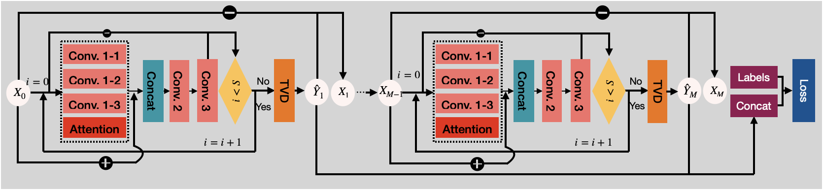
Figure 1: Graphic illustration of the network structure of RRCNN⁺.

The overall architecture of RRCNN⁺ is shown in Fig. 1. The pseudocode of RRCNN⁺ is reported in Algorithm 2 of the supplementary material. Compared to RRCNN, the improvements of RRCNN⁺ are reflected in two aspects. First, three convolutions with different kernel scales and an attention layer are carried out, their outputs and shared input are concatenated as the input of the Conv. 2 layer. Second, TVD is added in front of each IMF. The improvements are called the multi-scale convolutional attention and TVD modules, respectively, where the former enhances the adaptability and the diversity of the extracted features, while the latter obtains smooth components that are more meaningful from a physical perspective.

IV Experiments

We first evaluate the TVD and multi-scale convolutional attention modules that are adopted in RRCNN⁺. For the convenience of notation, we denote the models improved by TVD and multi-scale convolutional attention as RRCNN_TVD and RRCNN_ATT, respectively. Then, RRCNN⁺ is also compared with the state-of-the-art methods, including EMD [3], EEMD [27], VMD [12], EWT [28], FDM [29], IF [30], INCMD [31], SYNSQ_CWT and SYNSQ_STFT [32]. Details of the experimental data, settings, and evaluation metrics are described in the supplementary material.

IV-A Are TVD and multi-scale convolutional attention effective?

To justify that TVD and multi-scale convolutional attention modules are effective, we first compare RRCNN_TVD, RRCNN_ATT and RRCNN⁺ with RRCNN on both training and validation datasets of Dataset_1 and Dataset_2. The results, measured by MAE (mean absolute error), RMSE (root mean squared error), MAPE (mean absolute percentage error) and TV (total variation), are listed in Table I. We obtain the following findings: (i) For the vast majority of cases of both training and validation sets of Dataset_1 and Dataset_2, TVD and multi-scale convolutional attention effectively improve the performance over RRCNN. (ii) Combining TVD and multi-scale convolutional attention, i.e., RRCNN⁺, improves performance over RRCNN in all cases. In addition, we examine the smoothness by comparing the TV norm. The TV values for the components generated by RRCNN⁺ are essentially the closest to those of the true components.

TABLE I: Results of different models on training and validation sets of Dataset_1 and Dataset_2.

Dataset		Method	Error			Smoothness
			MAE	RMSE	MAPE	TV
Dataset_1	Training	True	0	0	0	1139.7
		RRCNN	0.0299	0.0517	0.4967	1104.3
		RRCNN_TVD	0.0219	0.0408	0.4904	1081.8
		RRCNN_ATT	0.0156	0.0332	0.3753	1133.7
		RRCNN+	0.0156	0.0307	0.3429	1133.8
	Validation	True	0	0	0	1162.9
		RRCNN	0.0283	0.0567	0.5187	1130.7
		RRCNN_TVD	0.0227	0.0453	0.4316	1105.8
		RRCNN_ATT	0.0150	0.0353	0.3937	1160.2
		RRCNN+	0.0148	0.0329	0.3628	1156.4
Dataset_2	Training	True	0	0	0	1139.7
		RRCNN	0.0362	0.0564	0.5510	1071.8
		RRCNN_TVD	0.0348	0.0543	0.7784	1062.8
		RRCNN_ATT	0.0334	0.0529	0.5043	1071.6
		RRCNN+	0.0290	0.0482	0.5280	1118.8
	Validation	True	0	0	0	1162.9
		RRCNN	0.0366	0.0593	0.5555	1088.1
		RRCNN_TVD	0.0341	0.0549	0.4964	1080.5
		RRCNN_ATT	0.0327	0.0534	0.6524	1091.5
		RRCNN+	0.0269	0.0435	0.4593	1140.7

To test the generalization capability of both modules, two signals not contained in both datasets are constructed. The first one is $x_{1}(t)=\cos(6.4\pi t)+\cos(5\pi t)$, where $\cos(6.4\pi t)$ and $\cos(5\pi t)$ are denoted as the components $c_{1}$ and $c_{2}$ of $x_{1}$, respectively. The frequencies of $c_{1}$ and $c_{2}$ are very close, which makes $x_{1}$ can be used to evaluate the deep-learning-based models trained on Dataset_1. The second signal is $x_{2}(t)=\cos\left(8\pi t+2t^{2}+\cos(t)\right)+\cos(5\pi t)+\varepsilon(t)$, where $\cos\left(8\pi t+2t^{2}+\cos(t)\right)$ and $\cos(5\pi t)$ are called the components $c_{1}$ and $c_{2}$ of $x_{2}$, respectively, $\varepsilon(t)$ is additive Gaussian noise with $\text{SNR}=15dB$. $x_{2}$ contains stronger noise than that added to the signals in Dataset_2, and it is used to test against the trained deep-learning-based models on Dataset_2.

Results of $x_{1}$, $x_{2}$ are given in Table II and Fig. 2. In Table II, we observe that the results obtained by RRCNN_TVD, RRCNN_ATT and RRCNN⁺ are always better, measured by error metrics, than that of RRCNN, which indicates the effectiveness of introducing TVD and multi-scale convolutional attention. From the TV norm comparison, we see that RRCNN_TVD, RRCNN_ATT and RRCNN⁺ improve the results obtained by RRCNN, except in one case on $c_{1}$ of $x_{2}$, where the TV norm of RRCNN is the closest to that of true component. By looking closely at Fig. 2, we found that RRCNN_TVD, RRCNN_ATT and RRCNN⁺ greatly improve the performance of RRCNN at the peaks and troughs.

TABLE II: Results of $x_{1}$, $x_{2}$ by deep-learning-based models trained on Dataset_1 and Dataset_2, respectively.

Signal		Method	Error			Smoothness
			MAE	RMSE	MAPE	TV
$x_{1}$	$c_{1}$	True	0	0	0	76.6830
		RRCNN	0.1781	0.2386	1.0592	66.4462
		RRCNN_TVD	0.1502	0.2003	0.7016	65.5484
		RRCNN_ATT	0.1550	0.1999	0.9284	69.0337
		RRCNN+	0.1462	0.1903	0.6798	65.6757
	$c_{2}$	True	0	0	0	59.9961
		RRCNN	0.0938	0.1323	0.5310	62.0982
		RRCNN_TVD	0.0655	0.0788	0.4929	59.0212
		RRCNN_ATT	0.1549	0.1902	1.1313	56.1674
		RRCNN+	0.0882	0.1175	0.4167	57.8752
$x_{2}$	$c_{1}$	True	0	0	0	141.7220
		RRCNN	0.1170	0.1604	2.0179	144.3518
		RRCNN_TVD	0.1050	0.1364	2.7891	134.9686
		RRCNN_ATT	0.0796	0.1092	1.2263	146.0654
		RRCNN+	0.0643	0.0872	1.1104	135.8261
	$c_{2}$	True	0	0	0	59.9961
		RRCNN	0.0930	0.1169	0.4770	63.7375
		RRCNN_TVD	0.0636	0.0830	0.3456	61.3893
		RRCNN_ATT	0.0631	0.0817	0.4748	60.8893
		RRCNN+	0.0442	0.0543	0.2591	61.5314

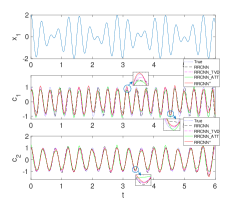
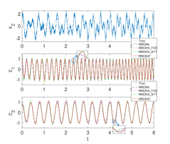
Figure 2: Results of $x_{1}$, $x_{2}$ by deep-learning-based models trained on Dataset_1, Dataset_2, respectively. Left: $x_{1}$; Right: $x_{2}$.

IV-B Can RRCNN⁺ outperform the state-of-the-art models?

RRCNN⁺ is also compared with existing methods, including EMD, EEMD, VMD, EWT, FDM, IF, INCMD, SYNSQ_CWT, SYNSQ_STFT, RRCNN, RRCNN_TVD and RRCNN_ATT. Again, we take $x_{1}$ and $x_{2}$ that are constructed in Section IV-A as the test signals.

The results obtained by different methods are shown in Table VI of the supplementary material. Here we only list the results of the true and the obtained components by the top three methods in Table VI. We find that: (i) Since the frequencies of the constituent components of $x_{1}$ are very close, and $x_{2}$ is disturbed by high level noise, some existing methods, such as EWT, FDM and VMD for $x_{1}$, and EEMD and SYNSQ_STFT for $x_{2}$ have a hard time distinguishing the two components. Other methods, like EWT, INCMD and SYNSQ_CWT only show relatively accurate components on $x_{2}$. (ii) Deep-learning-based methods are generally impressive on both $x_{1}$ and $x_{2}$.

The components and the corresponding time-frequency distributions by the top three models are depicted in Fig. 4 in the supplementary material. Here, we only depict time-frequency distributions of true and the components of RRCNN⁺ in Fig. 3. Although the time-frequency information of non-stationary signals is not considered in RRCNN⁺, its result is still relatively reasonable. We expect that a more accurate time-frequency distribution will be yielded when time-frequency information is incorporated into the model.

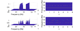
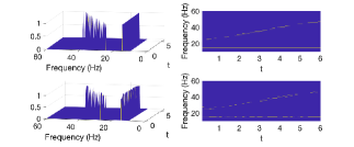
Figure 3: Time-frequency distribution by IMFogram [33] for the true (top) and resulting components (bottom) of $x_{1}$ (left) and $x_{2}$ (right) by RRCNN⁺.

TABLE III: Results of $x_{1}$ and $x_{2}$ by top three methods, where deep learning based models for $x_{1}$ and $x_{2}$ are trained based on Dataset_1 and Dataset_2, respectively.

Signal		Method	Error			Smoothness
			MAE	RMSE	MAPE	TV
$x_{1}$	$c_{1}$	True	0	0	0	76.6830
		SYNSQ_CWT	0.1566	0.2684	0.5083	61.7489
		RRCNN_TVD	0.1502	0.2003	0.7016	65.5484
		RRCNN+	0.1462	0.1903	0.6798	65.6757
	$c_{2}$	True	0	0	0	59.9961
		SYNSQ_CWT	0.0600	0.0927	0.1596	55.1799
		RRCNN_TVD	0.0655	0.0788	0.4929	59.0212
		RRCNN+	0.0882	0.1175	0.4167	57.8752
$x_{2}$	$c_{1}$	True	0	0	0	141.7220
		RRCNN_TVD	0.1050	0.1364	2.7891	134.9686
		RRCNN_ATT	0.0796	0.1092	1.2263	146.0654
		RRCNN+	0.0643	0.0872	1.1104	135.8261
	$c_{2}$	True	0	0	0	59.9961
		RRCNN_TVD	0.0636	0.0830	0.3456	61.3893
		RRCNN_ATT	0.0631	0.0817	0.4748	60.8893
		RRCNN+	0.0442	0.0543	0.2591	61.5314

V Conclusion

We recalled RRCNN and introduced RRCNN⁺, deep-learning-based methods for non-stationary signal decomposition. We demonstrated that by introducing the multi-scale convolutional attention and TVD, RRCNN⁺ improves the performance of RRCNN, and overcomes some of its limitations.

Yet, RRCNN⁺ has some limitations too. For example, its network does not take into account the time-frequency information of the signal, which leads to the lack of time-frequency physical meaning in the results. RRCNN⁺ is a supervised learning model that needs to assign a label to each training data. It is not easy to extend this approach to real signals because labels for real signals are difficult to obtain. We plan to further address these issues in future work.

Supplementary Material

To facilitate the reading with the main paper, the section numbers and titles are consistent with those in the main paper.

III RRCNN⁺

The solution of $\text{TVD}(\hat{Y})$ and the process of RRCNN⁺ are given in Algorithm 1-2, respectively.

Algorithm 1 Solution of $\text{TVD}(\hat{Y})$

  $Y=\hat{Y}$

  for $i=1,\ldots,Nit$ do

     ${\bf F}=diag\left(abs({\bf D}Y)/\lambda\right)+{\bf D}{\bf D}^{\top}$

     $Y=Y-{\bf D}^{\top}{\bf F}^{-1}{\bf D}\hat{Y}$

  end for

Algorithm 2 RRCNN⁺

0:  Pre-decomposed signal $X\in\mathbb{R}^{N}$, number of IMFs $M$.

0:  IMFs and residue of $X$

  for $m=1\ldots,M$ do

     $X_{0}=X$

     for $s=1,\dots,S$ do

        $X_{k}=\sigma(X\ast{W}_{1k})$

        $X_{att}=\text{Attention}(X)$

        $\hat{X}=\sigma\left(\text{Concat}([X,X_{1},X_{2},X_{3},X_{att}])\ast{W}_{2}\right)\ast{\tilde{W}}_{3}$

        $X=X_{0}-\hat{X}$

     end for

     $\hat{Y}_{m}=\text{TVD}(X)$ according to Alg. 1

     $X=X_{0}-\hat{Y}_{m}$

  end for

  $\hat{\bf Y}=\{\hat{Y}_{m}\}_{m=1}^{M}$, the final $X$ are IMFs and residue.

IV Experiments

• Evaluation metrics

Table IV lists the metrics for evaluating the results, where MAE (Mean Absolute Error), RMSE (Root Mean Squared Error) and MAPE (Mean Absolute Percentage Error) are employed to measure the errors between the predicted vector $\hat{Y}\in\mathbb{R}^{N}$ and label $Y\in\mathbb{R}^{N}$, TV (Total Variation) is used to measure the smoothness of predicted component $\hat{Y}\in\mathbb{R}^{N}$. In particular, the smaller the values of MAE, RMSE and MAPE, the better the performance of the model. As a measurement of smoothness, the smaller the value of TV, the smoother the predicted component, so it cannot be used as an intuitive criterion to judge the result. In general, the closer the TV value of the predicted component is to that of the true component, the better the result is to a certain extent.

TABLE IV: Evaluation metrics

Metric	MAE	RMSE	MAPE	TV
Expression	$\frac{\|\hat{Y}-Y\|_{1}}{N}$	$\sqrt{\frac{\|\hat{Y}-Y\|_{2}^{2}}{N}}$	$\frac{\sum_{t=1}^{N}|\frac{\hat{Y}_{t}-Y_{t}}{Y_{t}}|}{N}$	$\|{\bf D}\hat{Y}\|_{1}$

• Experimental data

Similarly to what we did to evaluate RRCNN, we construct the datasets by artificially synthesizing signals to evaluate RRCNN⁺. The first dataset, called Dataset_1, is composed of the signals of two categories: some signals are composed of a mono-component signal and a zero signal, and the others are of two mono-components with close frequencies. The former is to evaluate RRCNN⁺ in decomposing the zero local average of the mono-component signal; the latter is to enable RRCNN⁺ to decompose signals with close frequencies, which is the main factor causing the mode mixing issue. Secondly, to verify the robustness of RRCNN⁺, we construct another dataset, called Dataset_2, that consists of the signals in Dataset_1 perturbed with the additive Gaussian noise with the signal-to-noise ratio (SNR) as 25dB. The inputs (a.k.a. features) and labels of Dataset_1, Dataset_2 are given in Table V.

Each dataset is divided into the training and validation sets with a ratio of $8:2$, where the training set is used to train the deep-learning-based model, and the validation set is to select the hyper-parameters for the model.

TABLE V: Inputs (features) and labels of the artificially constructed datasets, where $t\in[0,6]$ and $\varepsilon(t)$ denotes the additive Gaussian noise with SNR as $25dB$.

Dataset	$c_{2}$	$c_{1}$	Feature	Label	Note
Dataset_1	$\cos(k\pi t)$	$\cos((k+1.5)\pi t)$	$c_{1}+c_{2}$	$[c_{1},c_{2}]$	$k=5,6,\ldots,14$
		$\cos((k+1.5)\pi t+t^{2}+\cos(t))$
	$0$	$\cos((k+1.5)\pi t)$
		$\cos((k+1.5)\pi t+t^{2}+\cos(t))$
	$\cos(k\pi t)$	$\cos(kl\pi t)$	$c_{1}+c_{2}$	$[c_{1},c_{2}]$	$k=5,6,\ldots,14$
		$\cos(kl\pi t+t^{2}+\cos(t))$
	$0$	$\cos(kl\pi t)$			$l=2,3,\ldots,19$
		$\cos(kl\pi t+t^{2}+\cos(t))$
Dataset_2	$\cos(k\pi t)$	$\cos((k+1.5)\pi t)$	$c_{1}+c_{2}+\varepsilon(t)$	$[c_{1},c_{2}]$	$k=5,6,\ldots,14$
		$\cos((k+1.5)\pi t+t^{2}+\cos(t))$
	$0$	$\cos((k+1.5)\pi t)$
		$\cos((k+1.5)\pi t+t^{2}+\cos(t))$
	$\cos(k\pi t)$	$\cos(kl\pi t)$	$c_{1}+c_{2}+\varepsilon$	$[c_{1},c_{2}]$	$k=5,6,\ldots,14$
		$\cos(kl\pi t+t^{2}+\cos(t))$
	$0$	$\cos(kl\pi t)$			$l=2,3,\ldots,19$
		$\cos(kl\pi t+t^{2}+\cos(t))$

• Experimental settings

For the experiments related to EMD (Empirical Mode Decomposition), EEMD (Ensemble Empirical Mode Decomposition), VMD (Variational Mode Decomposition), EWT (Empirical Wavelet Transformer), FDM (Fourier Decomposition Method), IF (Iterative Filtering), SYNSQ_CWT (Continuous Wavelet Transform based Synchrosqueezing) and SYNSQ_STFT (Short-Time Fourier Transform based Synchrosqueezing), they are implemented in Matlab R2022a on Mac Ventura 13.3.1 operating system with processor 2.3 GHz Dual-Core Intel Core i5. For the experiments related to INCMD, RRCNN, RRCNN_TVD, RRCNN_ATT and RRCNN⁺, they are performed in Python 3.9.12 on Centos 7.4.1708 operating system with GPU (NVIDIA A30 and NVIDIA A100). The deep-learning-based models, RRCNN, RRCNN_TVD, RRCNN_ATT and RRCNN⁺ are achieved under the Tensorflow platform with version: 2.5.0, which is an end-to-end open source platform for machine learning. The codes of RRCNN_TVD, RRCNN_ATT and RRCNN⁺ will be released on Github (https://github.com/zhoudafa08/RRCNN+) once the paper is accepted.

IV-B Can RRCNN⁺ outperform the state-of-the-art models?

The results of all models are listed in Table VI. And the resulting components and its time-frequency distribution of the top three models in terms of overall performance in Table VI are depicted in Fig. 4.

TABLE VI: Errors and smoothness of $x_{1}$ and $x_{2}$ by different models, where RRCNN, RRCNN_TVD, RRCNN_ATT and RRCNN⁺ for $x_{1}$ and $x_{2}$ are trained based on Dataset_1 and Dataset_2, respectively. The best and second best results are marked by bold and underline, respectively.

Signal	Method	$c_{1}$				$c_{2}$
		Error			Smoothness	Error			Smoothness
		MAE	RMSE	MAPE	TV	MAE	RMSE	MAPE	TV
$x_{1}$	True	0	0	0	76.6830	0	0	0	59.9961
	EMD	0.2113	0.2434	1.4070	78.9678	0.2378	0.2793	1.8732	45.6324
	VMD	0.3823	0.4297	0.8779	32.7923	0.3758	0.4240	1.9308	62.7881
	EWT	0.6379	0.7078	1.0006	0.9406	0.6379	0.7078	3.6569	90.7875
	FDM	0.6369	0.7102	3.6148	90.8130	0.6368	0.7101	1.2510	5.4819
	IF	0.2447	0.2928	0.9755	51.8706	0.2932	0.3267	0.5857	32.4619
	INCMD	0.1658	0.2084	1.0495	83.4392	0.1783	0.2142	1.1291	46.2430
	SYNSQ_CWT	0.1566	0.2684	0.5083	61.7489	0.0600	0.0927	0.1596	55.1799
	SYNSQ_STFT	0.1859	0.2359	0.9761	85.7133	0.1853	0.2397	1.2491	69.0358
	RRCNN	0.1781	0.2386	1.0592	66.4462	0.0938	0.1323	0.5310	62.0982
	RRCNN_TVD	0.1502	0.2003	0.7016	65.5484	0.0655	0.0788	0.4929	59.0212
	RRCNN_ATT	0.1550	0.1999	0.9284	69.0337	0.1549	0.1902	1.1313	56.1674
	RRCNN+	0.1462	0.1903	0.6798	65.6757	0.0882	0.1175	0.4167	57.8752
$x_{2}$	True	0	0	0	141.7220	0	0	0	59.9961
	EMD	0.3774	0.6096	3.5358	91.2037	0.2415	0.3763	1.3900	49.1055
	EEMD	0.5538	0.7728	4.9839	74.1906	0.4324	0.5594	1.3101	26.7755
	VMD	0.1718	0.2640	0.5581	120.7649	0.1609	0.2553	1.2251	70.1177
	EWT	0.4540	0.5709	0.9942	43.5686	0.0467	0.0766	0.4547	61.4683
	FDM	0.1450	0.2065	1.0558	136.3556	0.1432	0.2009	1.0893	63.8787
	IF	0.2481	0.3496	0.7144	80.8994	0.0470	0.0677	0.3768	58.1244
	INCMD	0.7973	0.8983	5.8560	106.5416	0.0480	0.0682	0.4173	58.8118
	SYNSQ_CWT	0.5560	0.6202	1.2871	23.4034	0.0535	0.1004	0.1254	55.6807
	SYNSQ_STFT	0.4572	0.5694	3.2621	105.5599	0.3662	0.4394	0.6649	93.6073
	RRCNN	0.1170	0.1604	2.0179	144.3518	0.0930	0.1169	0.4770	63.7375
	RRCNN_TVD	0.1050	0.1364	2.7891	134.9686	0.0636	0.0830	0.3456	61.3893
	RRCNN_ATT	0.0796	0.1092	1.2263	146.0654	0.0631	0.0817	0.4748	60.8893
	RRCNN+	0.0643	0.0872	1.1104	135.8261	0.0442	0.0543	0.2591	61.5314

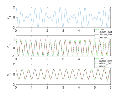
(a) Components of $x_{1}$ by SYNSQ_CWT, RRCNN_TVD and RRCNN⁺.

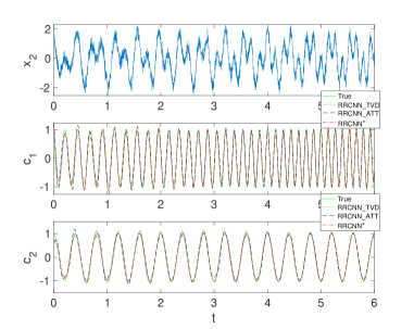
(b) Components of $x_{2}$ by RRCNN_TVD, RRCNN_ATT and RRCNN⁺.

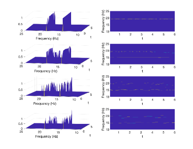
(c) Time-frequency distributions by IMFogram for the components of $x_{1}$. From top to bottom: True, SYNSQ_CWT, RRCNN_TVD and RRCNN⁺.

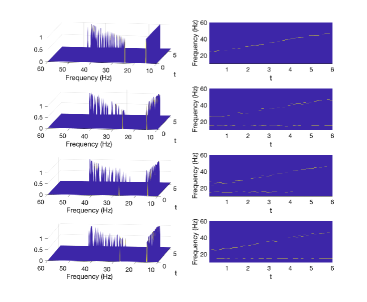
(d) Time-frequency distributions by IMFogram for the components of $x_{2}$. From top to bottom: True, RRCNN_TVD, RRCNN_ATT and RRCNN⁺.

Figure 4: Results of $x_{1}$ and $x_{2}$ by the top three models in terms of the overall performance in Table VI.

References

- [1] T. W. Körner, Fourier analysis. Cambridge university press, 2022.
- [2] D. F. Walnut, An introduction to wavelet analysis. Springer Science & Business Media, 2002.
- [3] N. E. Huang, Z. Shen, S. R. Long, M. C. Wu, H. H. Shih, Q. Zheng, N. C. Yen, C. C. Tung, and H. H. Liu, “The empirical mode decomposition and the Hilbert spectrum for nonlinear and non-stationary time series analysis,” Proceedings of the Royal Society of London. Series A: Mathematical, Physical and Engineering Sciences, vol. 454, no. 1971, pp. 903–995, 1998.
- [4] J. S. Smith, “The local mean decomposition and its application to EEG perception data,” Journal of the Royal Society Interface, vol. 2, no. 5, pp. 443–454, 2005.
- [5] H. Hong, X. Wang, and Z. Tao, “Local integral mean-based sifting for empirical mode decomposition,” IEEE Signal Processing Letters, vol. 16, no. 10, pp. 841–844, 2009.
- [6] E. Deléchelle, J. Lemoine, and O. Niang, “Empirical mode decomposition: an analytical approach for sifting process,” IEEE Signal Processing Letters, vol. 12, no. 11, pp. 764–767, 2005.
- [7] S. D. El Hadji, R. Alexandre, and A.-O. Boudraa, “Analysis of intrinsic mode functions: A PDE approach,” IEEE Signal Processing Letters, vol. 17, no. 4, pp. 398–401, 2009.
- [8] L. Lin, Y. Wang, and H. Zhou, “Iterative filtering as an alternative algorithm for empirical mode decomposition,” Advances in Adaptive Data Analysis, vol. 1, no. 04, pp. 543–560, 2009.
- [9] A. Cicone and E. Pellegrino, “Multivariate fast iterative filtering for the decomposition of nonstationary signals,” IEEE Transactions on Signal Processing, vol. 70, pp. 1521–1531, 2022.
- [10] A. Cicone and H. Zhou, “Multidimensional iterative filtering method for the decomposition of high–dimensional non–stationary signals,” Numerical Mathematics: Theory, Methods and Applications, vol. 10, no. 2, pp. 278–298, 2017.
- [11] T. Y. Hou and Z. Shi, “Sparse time-frequency representation of nonlinear and nonstationary data,” Science China Mathematics, vol. 56, pp. 2489–2506, 2013.
- [12] K. Dragomiretskiy and D. Zosso, “Variational mode decomposition,” IEEE Transactions on Signal Processing, vol. 62, no. 3, pp. 531–544, 2013.
- [13] N. ur Rehman and H. Aftab, “Multivariate variational mode decomposition,” IEEE Transactions on Signal Processing, vol. 67, no. 23, pp. 6039–6052, 2019.
- [14] S. Yu, J. Ma, and S. Osher, “Geometric mode decomposition,” Inverse Problems & Imaging, vol. 12, no. 4, 2018.
- [15] F. Zhou, L. Yang, H. Zhou, and L. Yang, “Optimal averages for nonlinear signal decompositions—another alternative for empirical mode decomposition,” Signal Processing, vol. 121, pp. 17–29, 2016.
- [16] S. Peng and W.-L. Hwang, “Null space pursuit: An operator-based approach to adaptive signal separation,” IEEE Transactions on Signal processing, vol. 58, no. 5, pp. 2475–2483, 2010.
- [17] T. Oberlin, S. Meignen, and V. Perrier, “An alternative formulation for the empirical mode decomposition,” IEEE Transactions on Signal Processing, vol. 60, no. 5, pp. 2236–2246, 2012.
- [18] N. Pustelnik, P. Borgnat, and P. Flandrin, “Empirical mode decomposition revisited by multicomponent non-smooth convex optimization,” Signal Processing, vol. 102, pp. 313–331, 2014.
- [19] F. Zhou, A. Cicone, and H. Zhou, “Rrcnn: A novel signal decomposition approach based on recurrent residue convolutional neural network,” arXiv preprint arXiv:2307.01725, 2023.
- [20] Y. Fu, J. Wu, Y. Hu, M. Xing, and L. Xie, “Desnet: A multi-channel network for simultaneous speech dereverberation, enhancement and separation,” in 2021 IEEE Spoken Language Technology Workshop (SLT). IEEE, 2021, pp. 857–864.
- [21] Z. Cui, W. Chen, and Y. Chen, “Multi-scale convolutional neural networks for time series classification,” arXiv preprint arXiv:1603.06995, 2016.
- [22] A. Vaswani, N. Shazeer, N. Parmar, J. Uszkoreit, L. Jones, A. N. Gomez, Ł. Kaiser, and I. Polosukhin, “Attention is all you need,” Advances in neural information processing systems, vol. 30, 2017.
- [23] K. He, X. Zhang, S. Ren, and J. Sun, “Deep residual learning for image recognition,” in Proceedings of the IEEE Conference on Computer Vision and Pattern Recognition, 2016, pp. 770–778.
- [24] L. I. Rudin, S. Osher, and E. Fatemi, “Nonlinear total variation based noise removal algorithms,” Physica D: nonlinear phenomena, vol. 60, no. 1-4, pp. 259–268, 1992.
- [25] M. A. Figueiredo, J. B. Dias, J. P. Oliveira, and R. D. Nowak, “On total variation denoising: A new majorization-minimization algorithm and an experimental comparisonwith wavalet denoising,” in 2006 International Conference on Image Processing. IEEE, 2006, pp. 2633–2636.
- [26] I. Selesnick, “Total variation denoising (an mm algorithm),” NYU Polytechnic School of Engineering Lecture Notes, vol. 32, 2012.
- [27] Z. Wu and N. E. Huang, “Ensemble empirical mode decomposition: A noise-assisted data analysis method,” Advances in Adaptive Data Analysis, vol. 1, no. 01, pp. 1–41, 2009.
- [28] J. Gilles, “Empirical wavelet transform,” IEEE Transactions on Signal Processing, vol. 61, no. 16, pp. 3999–4010, 2013.
- [29] P. Singh, S. D. Joshi, R. K. Patney, and K. Saha, “The Fourier decomposition method for nonlinear and non-stationary time series analysis,” Proceedings of the Royal Society A: Mathematical, Physical and Engineering Sciences, vol. 473, no. 2199, p. 20160871, 2017.
- [30] A. Cicone, J. Liu, and H. Zhou, “Adaptive local iterative filtering for signal decomposition and instantaneous frequency analysis,” Applied and Computational Harmonic Analysis, vol. 41, no. 2, pp. 384–411, 2016.
- [31] G. Tu, X. Dong, S. Chen, B. Zhao, L. Hu, and Z. Peng, “Iterative nonlinear chirp mode decomposition: A Hilbert-Huang transform-like method in capturing intra-wave modulations of nonlinear responses,” Journal of Sound and Vibration, vol. 485, p. 115571, 2020.
- [32] I. Daubechies, J. Lu, and H.-T. Wu, “Synchrosqueezed wavelet transforms: An empirical mode decomposition-like tool,” Applied and Computational Harmonic Analysis, vol. 30, no. 2, pp. 243–261, 2011.
- [33] P. Barbe, A. Cicone, W. S. Li, and H. Zhou, “Time-frequency representation of nonstationary signals: the imfogram,” Pure and Applied Functional Analysis, vol. 7, no. 1, pp. 27–39, 2022.