Maximizing Quantum-to-Classical Information Transfer in Four-Dimensional
Scanning Transmission Electron Microscopy

Abstract

We analyze the transfer of quantum information to detected classical information in four-dimensional scanning transmission electron microscopy. In estimating the moduli and phases of the Fourier coefficients of the sample’s electrostatic potential, we find that near-optimum information transfer is achieved by a delocalized speckled probe, which attains about half of the available quantum Fisher information. The quantum limit itself is precluded due to detecting the scattering in momentum space. We compare with direct phase-contrast imaging, where a Zernike phase condition attains the quantum limit for all spatial frequencies admitted by the optical system. Our conclusions also apply to other forms of coherent scalar radiation, such as visible light and x-rays.

Quests persist to develop ever-more sensitive imaging techniques to probe the structure of materials down to the atomic level. Ultra-high sensitivity becomes absolutely mandatory when studying samples such as quantum materials and radiation-sensitive materials. For radiation-based imaging techniques, dose efficiency is of primary importance, i.e., for a given “radiation budget,” what precision can be achieved in measuring the material’s properties of interest? All quests for sensitivity/precision are ultimately bound by the laws of quantum mechanics. Such limitations are most famously known in the form of the Heisenberg uncertainty relations. However, there now exists a considerably more general formalism known as quantum estimation theory (see Liu et al. (2020)), which can offer significant insights into the limitations of a given technique, and provide reasons why certain techniques enable maximimum dose efficiency.

Here, we apply the formalism to analyze and optimize the sensitivity of four-dimensional scanning transmission electron microscopy (4D-stem) (see Ophus (2019)), which has emerged as a favored technique for imaging the atomic structures of a wide variety of materials, including radiation-sensitive materials. The technique permits a range of simultaneous imaging modes, is capable of deep sub-Ångström resolution, and provides sensitivity to both light and heavy elements. The very high spatial resolution resides in the fact that 4D-stem is an indirect imaging technique, whereby an electron beam is scanned across the sample, and for each beam position the distribution of scattering is captured by a pixellated detector in momentum (diffraction) space, producing a four-dimensional dataset. The image itself never physically exists but is reconstructed via computation.

Our quantum estimation theory-based analysis reveals that, when optimized, 4D-stem can attain about half of the available quantum Fisher information, meaning that, for a given level of precision, it requires about twice the minimum electron dose permitted by quantum mechanics. For an arbitrary spatial frequency, we find that near-optimum information transfer is achieved by a delocalized speckled probe. Preclusion of the quantum limit itself is a consequence of detection in momentum space, and it applies to 4D-stem imaging generally, including bright-field, dark-field, differential-phase-contrast Shibata et al. (2012), center-of-mass Müller et al. (2014); *Yucelen-etal2018, matched-illumination Ophus et al. (2016), symmetry-based Krajnak and Etheridge (2020), and ptychographic Nellist et al. (1995); *Putkunz-etal2012; *Jiang-etal2018; *Song-etal2019; *Zhou-etal2020; *Schloz-etal2020; *ChenMuller-etal2020; *Li-etal2022 imaging.

We compare the dose efficiency of 4D-stem with phase-contrast transmission electron microscopy (tem), the standard (direct) imaging modality for biological materials and whose collection efficiency is similar. Under the Zernike phase condition, phase-contrast tem provides the greatest sensitivity, in that it enables the quantum limit for all spatial frequencies admitted by the optics. While 4D-stem generally cannot attain the quantum limit, it yields information on spatial frequencies well beyond those accessible by phase-contrast tem.

Background.—We will consider the 4D-stem and tem optical setups in Fig. 1, where beams of $\sim$100 keV electrons pass through an electron-transparent sample. In 4D-stem, a pixellated detector captures the diffracted intensity distribution for each beam position, and the resulting four-dimensional dataset is used to reconstruct an image. In tem, we assume fixed parallel illumination at normal incidence, and a pixellated detector in the image plane captures the image directly.

We assume that the experimental goal is to estimate, simultaneously, the moduli and phases of the Fourier coefficients of the sample’s electrostatic potential. For materials structure determination, the phases of the Fourier coefficients are usually of particular importance, though we shall mostly treat the moduli and phases on equal footing. The moduli and phases form a set of $P$ real parameters $\lambda_{1},\dots,\lambda_{P}$. We assume that all other parameters, such as those characterizing the optics, are already known with sufficient accuracy.

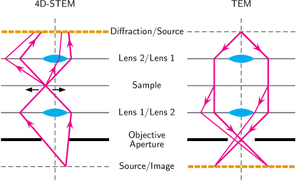
Figure 1: Electron-optical geometries for 4D-stem (left) and phase-contrast tem (right). These reciprocally-related geometries have similar collection efficiencies, and we assume an equivalent degree of aberration control up to the field angles admitted by the objective aperture.

Quantum-to-Classical Fisher information.—The quantum Fisher information matrix (qfim), a $P\times P$ matrix denoted $J$, is a key quantity in quantum estimation theory Liu et al. (2020). $J$ is a quantum analogue of the usual (classical) Fisher information matrix (cfim), a $P\times P$ matrix denoted $I$. In the regime of asymptotic statistics, $I$ and $J$ are related to the attainable variance in the (unbiased) estimation of a parameter $\lambda_{\mu}$ via the inequality chain Braunstein and Caves (1994); *Braunstein-etal1996

$${\mathrm{var}[\lambda_{\mu}]}\geq{I}^{-1}_{\mu\mu}\geq{J}^{-1}_{\mu\mu}.$$ (1)

$I^{-1}_{\mu\mu}$ is the $\mu$th diagonal element of the inverse matrix $I^{-1}$, and analogously for $J^{-1}_{\mu\mu}$. Thus, $I^{-1}_{\mu\mu}$ gives the Cramer-Rao lower bound which applies to any (unbiased) estimator, and $J^{-1}_{\mu\mu}$ provides a lower bound for $I^{-1}_{\mu\mu}$. If both equalities are obtained for all parameters, i.e., ${\mathrm{var}[\lambda_{\mu}]}={J}^{-1}_{\mu\mu}$ $\forall\mu$, then then the simultaneous quantum limit is achieved. The first equality can be achieved using a suitable estimator, such as a maximum-likelihood estimator. However, the second equality can be achieved only under optimum experimental conditions.

For a pure quantum state ${|\psi\rangle}$, $J$ can be defined as Liu et al. (2020)

$$J_{\mu\nu}\equiv 4N\mathrm{Re}\,{{\langle\psi_{\mu}|}\hat{Q}{|\psi_{\nu}\rangle}},$$ (2)

where ${|\psi_{\mu}\rangle}\equiv\partial{|\psi\rangle}/\partial\lambda_{\mu}$, $\hat{Q}\equiv 1-{|\psi\rangle\langle\psi|}$ projects onto the orthogonal complement of ${|\psi\rangle}$, and $N$ is the number of independent repetitions of the experiment. In our context, $N$ is the number of beam electrons used.

To define the cfim elements $I_{\mu\nu}$, we assume that the detection of ${|\psi\rangle}$ is described by a projection-valued measure (pvm) specified by a complete set of projectors $\{{|\xi\rangle\langle\xi|}\}$. Each projector corresponds to a possible experimental outcome with probability $p(\xi)=|{\langle\xi|\psi\rangle}|^{2}$. In this case, $I_{\mu\nu}$ can be written in the form

$$I_{\mu\nu}=4N\sum_{\xi}\frac{\mathrm{Re}\{{\langle\psi_{\mu}|\xi\rangle}{\langle\xi|\psi\rangle}\}\mathrm{Re}\{{\langle\psi|\xi\rangle}{\langle\xi|\psi_{\nu}\rangle}\}}{{\langle\xi|\psi\rangle}{\langle\psi|\xi\rangle}}.$$ (3)

It is important to appreciate that, while $J$ involves the state ${|\psi\rangle}$, it does not involve the process of detection. By contrast, $I$ does also depend on the specifics of the detection process as represented by the pvm. Loosely, we can think of $J$ and $I$ as the “potential” and “actual” information, respectively. An experiment enables the quantum limit if $I=J$, which is possible if and only if Matsumoto (2002); *BaumgratzDatta2015; *Pezze-etal2017; Liu et al. (2020); *BelliardoGiovannetti2021

$${{\langle\psi|}{\big{[}\hat{H}_{\mu},\hat{H}_{\nu}\big{]}}{|\psi\rangle}}=0\quad\text{$\forall$ $\mu$ and $\nu$},$$ (4a)

$${\langle\psi|\xi\rangle}{{\langle\xi|}\hat{Q}{|\psi_{\mu}\rangle}}\in\mathbb{R}\quad\text{$\forall$ $\xi$ and $\mu$},$$ (4b)

where $\hat{H}_{\mu}$ is an Hermitian generator for $\lambda_{\mu}$.

In what follows, unless otherwise stated, we adopt the weak phase-object approximation (wpoa) whereby expressions are retained to leading order in the projected potential $\hat{V}$. The theory is not restricted to this approximation (see Ref. Dwyer (2023) for expressions pertaining to scattering conditions ranging from weak to strong). However, the simplicity of the wpoa allows analytical results which build intuition and pave the way for future work. In the wpoa, condition (4a) is always satisfied.

Our parameters.—In coordinate space, $\hat{V}$ can be written in the form

$$V(x)=\sum_{k}V(k)e^{2\pi ik\cdot x},$$ (5)

where the Fourier coefficients $V(k)$ obey $V(k)=\bar{V}(-k)$. Our parameters $\{\lambda_{\mu}\}$ are (a subset of) the Fourier moduli $|V(k_{\mu})|$ and phases $\phi(k_{\mu})\equiv\arg V(k_{\mu})$, whose spatial frequency $k_{\mu}$ lies in the half space defined by, e.g., $k_{x}>0$. The subscript $\mu$ on $k_{\mu}$ specifies that it is associated with the parameter set, and when needed we will further specify whether $\lambda_{\mu}$ means $|V(k_{\mu})|$ or $\phi(k_{\mu})$. We need the derivatives of $\hat{V}$ with respect to each $\lambda_{\mu}$. These derivatives, denoted $\hat{V}_{\mu}$, have the Fourier representations

$$V_{\mu}(k)=\begin{cases}\delta_{k,k_{\mu}}e^{i\phi(k_{\mu})}+\delta_{k,-k_{\mu}}e^{-i\phi(k_{\mu})},&\text{$\lambda_{\mu}=|V(k_{\mu})|$},\\ \delta_{k,k_{\mu}}iV(k_{\mu})-\delta_{k,-k_{\mu}}i\bar{V}(k_{\mu}),&\text{$\lambda_{\mu}=\phi(k_{\mu})$}.\end{cases}$$ (6)

Phase-contrast tem.—We let the incident state ${|\psi_{0}\rangle}$ be a plane wave at normal incidence, denoted ${|k_{0}\rangle}$ with $k_{0}=0$. We obtain

$${|\psi\rangle}=\hat{A}(1-i\hat{V}){|k_{0}\rangle},$$ (7)

where $\hat{A}$ is the (nonunitary) operator

$$\hat{A}\equiv\sum_{|k|\leq K}{|k\rangle}e^{-2\pi i\chi(k)}{\langle k|},$$ (8)

$\chi(k)$ is the aberration phase shift, and $K$ is the aperture radius. With the above expressions, we find that the qfim for phase-contrast tem is diagonal, with

$$J_{\mu\mu}=8N|V_{\mu}(k_{\mu})|^{2},\qquad\text{$|k_{\mu}|\leq K$}.$$ (9)

Here $J_{\mu\mu}$ is independent of the aberrations, and the corresponding quantum limits of precision in the moduli and phases are ${\mathrm{var}[|V(k_{\mu})|]}=1/8N$ and ${\mathrm{var}[\phi(k_{\mu})]}=1/8N|V(k_{\mu})|^{2}$, respectively. The latter variances obey a type of number-phase uncertainty Loudon (2000).

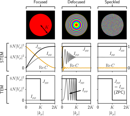
Figure 2: Quantum $J_{\mu\mu}$ and classical $I_{\mu\mu}$ Fisher information from 4D-stem and phase-contrast tem for three different aberration conditions. For each condition, the image shows an RGB plot of the aberration phase shift within the objective aperture, and the graphs show $J_{\mu\mu}$ and $I_{\mu\mu}$ for spatial frequencies up to $2K$. The lower-right graph shows tem results for the Zernike phase condition (ZPC). For stem, the real part of the autocorrelation $C$ is also shown (refer to right axis). The value of each curve at $|k_{\mu}|=2K$ persists at higher spatial frequencies. A $100$ keV beam energy, $20$ mrad aperture semi-angle, and $-100$ nm defocus are assumed (the latter value was chosen to be illustrative rather than optimum).

To determine whether the tem setup (Fig. 1) permits the quantum limit, we adopt for the pvm the complete set of projectors onto coordinate space $\{\frac{1}{M}{|x\rangle\langle x|}\}$ ($M$ is the number of points in the discretization of coordinate space). Alternatively to considering (4b), we can calculate the cfim for tem directly, which, for $|k_{\mu}|\leq K$, is

$$I_{\mu\mu}=4N|V_{\mu}(k_{\mu})|^{2}\left(1-\cos[2\pi(2\chi(0)-\chi(k_{\mu})-\chi(-k_{\mu}))]\right).$$ (10)

Fig. 2 (bottom row) compares $J_{\mu\mu}$ and $I_{\mu\mu}$ from tem phase-contrast imaging for different aberration conditions. For perfect focus $\chi(k)=0$, the image contains no information (as expected). A defocused condition enables the quantum limit for specific spatial frequencies. A Zernike phase condition $\chi(0)=\frac{1}{4},\chi(k\neq 0)=0$ enables the quantum limit for all spatial frequencies admitted by the optics Koppell et al. (2022); Dwyer (2023). An absolutely key point is that the Zernike condition makes ${|\psi\rangle}$ real (up to overall phase), so that ${|\psi\rangle}$ entails optimal interference with greatest possible sensitivity to the parameters of $\hat{V}$.

4D-stem.—We regard the 4D-stem experiment as $M$ independent quantum systems, for which the total quantum state is the tensor product

$${|\Psi\rangle}={|\psi(x_{1})\rangle}\otimes\cdots\otimes{|\psi(x_{M})\rangle},$$ (11)

where ${|\psi(x)\rangle}$ is a scattered state for which the incident beam was positioned at $x$ in the sample plane. We then use the fact that $J$ (and $I$) is additive with respect to independent systems Lu et al. (2012); *TothApellaniz2014. We also introduce the standard notation for the stem probe wave function ${\langle k|\psi_{0}(x)\rangle}=\psi_{0}(k)e^{-2\pi ik\cdot x}$, where

$$\psi_{0}(k)=\begin{cases}|\psi_{0}(k)|e^{-2\pi i\chi(k)}&\text{$|k|\leq K$},\\ 0&\text{otherwise}.\end{cases}$$ (12)

The qfim for stem is found to be diagonal, with

$$J_{\mu\mu}=8N|V_{\mu}(k_{\mu})|^{2}(1-|C(k_{\mu})|^{2}),$$ (13)

where $C(k_{\mu})=\sum_{k}\psi_{0}(k)\bar{\psi}_{0}(k+k_{\mu})$ is an autocorrelation with $C(0)=1$, and the spatial frequency $k_{\mu}$ is unrestricted. Moreover, (13) does depend on the aberrations through $C(k_{\mu})$. Maximum quantum Fisher information is obtained when $|C(k_{\mu})|=0$ (see discussion).

Notwithstanding the above remarks, 4D-stem does not enable the quantum limit for any spatial frequency. To see why, we adopt for the pvm the complete set of projectors onto Fourier space $\{{|k\rangle\langle k|}\}$, and we consider the reality condition (4b).

For wave vectors $k$ in the bright field, assuming that $|C(k_{\mu})|\approx 0$ (see above), (4b) becomes

$$\begin{split}&-i\bar{\psi}_{0}(k)\psi_{0}(k-k_{\mu})V_{\mu}(k_{\mu})e^{+2\pi ik_{\mu}\cdot x}\\ &+(+k_{\mu}\rightarrow-k_{\mu})\in\mathbb{R}\qquad\text{$\forall$ $x$, $|k|\leq K$ and $k_{\mu}$},\end{split}$$ (14)

where the notation in parentheses implies the preceding term with $+k_{\mu}$ replaced by $-k_{\mu}$. If $|k-k_{\mu}|\leq K$ and $|k+k_{\mu}|\leq K$ (the “tunable region,” see Fig. 3), then the two terms in (14) can combine to become real if the aberrations are such that $2\chi(k)-\chi(k-k_{\mu})-\chi(k+k_{\mu})=n+\tfrac{1}{2}$ for some integer $n$. On the other hand, if only $|k-k_{\mu}|\leq K$ or $|k+k_{\mu}|\leq K$ (the “untunable region,” see Fig. 3), then, due to the phase factor involving $x$, the relevant term will be real only for “half” (loosely speaking, though numerically correct) of the beam positions $x$, regardless of $k_{\mu}$ or $\chi$. Since the untunable region typically comprises a significant portion of the bright field, condition (14) cannot be satisfied.

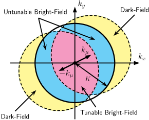
Figure 3: Bright- and dark-field contributions to the classical Fisher information for a spatial frequency $|k_{\mu}|\leq K$. Solid circle represents the stem objective aperture. Dashed circles represent the aperture displaced by $\pm k_{\mu}$. For $K<|k_{\mu}|\leq 2K$ (not shown) there is no tunable region. For $|k_{\mu}|>2K$ (not shown) there are only dark field contributions.

For $k$ in the dark field, condition (4b) takes the form

$$\begin{split}&\sum_{k^{\prime}}\bar{\psi}_{0}(k-k^{\prime})\bar{V}(k^{\prime})V_{\mu}(k_{\mu})\psi_{0}(k-k_{\mu})e^{-2\pi i(k^{\prime}-k_{\mu})\cdot x}\\ &+(+k_{\mu}\rightarrow-k_{\mu})\in\mathbb{R}\qquad\text{$\forall$ $x$, $|k|>K$ and $k_{\mu}$},\end{split}$$ (15)

where the notation implies a second summation with $+k_{\mu}$ replaced by $-k_{\mu}$. For a given $k$, only one of the summations can be in effect, which means that we cannot balance terms as before. Also notice that (15) is nonlinear in $\hat{V}$, which prevents us from obtaining general results. However, when multiple spatial frequencies $k^{\prime}$ contribute to the summation, then, owing to the phase factors involving $x$, there is again a general tendency for the condition to be satisfied for “half” of the beam positions, regardless of $k_{\mu}$ or $\chi$. (There are exceptions to this behavior: If the term $k^{\prime}=k_{\mu}$ dominates the summation, as it can when the stem probe convergence angle is small and there is little overlap of the diffraction discs, then (15) is always satisfied for $\lambda_{\mu}=|V(k_{\mu})|$, i.e., full modulus information, and never satisfied for $\lambda_{\mu}=\phi(k_{\mu})$, i.e., no phase information. The situation just described is the classic “phase problem.” Notwithstanding such cases, we take as the generic behavior, representative of 4D-stem, that when multiple spatial frequencies are present.)

Assuming the generic behavior of the dark field, we find that the complete cfim for 4D-stem is approximately diagonal, with diagonal elements given by

$$\begin{split}&I_{\mu\mu}\approx 4N|V_{\mu}(k_{\mu})|^{2}\\ &\times\big{(}1-\sum_{k}|\psi_{0}(k-k_{\mu})||\psi_{0}(k+k_{\mu})|\\ &\qquad\times\cos[2\pi(2\chi(k)-\chi(k-k_{\mu})-\chi(k+k_{\mu}))]\big{)}.\end{split}$$ (16)

Here $k_{\mu}$ is unrestricted. The terms inside the summation are the tunable bright-field contributions, which can range from fully additive (for the previously-stated condition on $\chi$) to fully subtractive (e.g., when $\chi=0$).

Fig. 2 compares $J_{\mu\mu}$ and $I_{\mu\mu}$ from 4D-stem for different aberration conditions. Perfect focus results in minimum $J_{\mu\mu}$ (since $|C|$ is maximized) and minimum $I_{\mu\mu}$ (since the tunable contributions are fully subtractive). A defocused condition dramatically improves $J_{\mu\mu}$ and improves $I_{\mu\mu}$ at specific spatial frequencies though not others. For an arbitrary spatial frequency $k_{\mu}$, a near-optimum $\chi$ is “random” on $[0,2\pi)$, giving $J_{\mu\mu}\approx 8N|V_{\mu}(k_{\mu})|^{2}$ and $I_{\mu\mu}\approx\frac{1}{2}J_{\mu\mu}$.

Discussion.—We have assumed the 4D-stem detector captures the entire scattering distribution, and found that the cfim is approximately half of the qfim. The cfim will be further reduced by a less-capable detector. Thus, 4D-stem, with its detector positioned in the diffraction plane, precludes the quantum limit in the simultaneous estimation of the Fourier moduli and phases. The latter statement is independent of the way in which the scattering data is processed, and thus applies to any 4D-stem technique. In fact, this conclusion applies even more broadly to similar techniques using other forms of coherent scalar radiation, such as visible light and x-rays.

In 4D-stem, the aberration-dependence of $J_{\mu\mu}$ can reduce the quantum information for $|k_{\mu}|\leq 2K$. For $k_{\mu}$ arbitrary, $J_{\mu\mu}$ is near-maximized by a “random” $\chi$, producing a delocalized speckled probe with expected autocorrelation ${\langle|C(k_{\mu})|^{2}\rangle}\leq 1/M_{K}$ ($M_{K}$ is the number of plane waves inside the aperture) and $I_{\mu\mu}\approx\frac{1}{2}J_{\mu\mu}$. Interestingly, there are several light and x-ray classical-imaging settings where such delocalized speckled illumination is advantageous (e.g., Ventalon and Mertz (2005); *Mudry2012; *Gatti2006; *Berujon2012; *Morgan2012). Low-autocorrelation sequences (e.g., Borwein and Ferguson (2005)) provide scope for even further optimization of $J_{\mu\mu}$. Note that $\chi$ must be effectively known to extract information $I_{\mu\mu}$ from the scattering data, and hence 4D-stem is an information encoding-decoding scheme. The $\chi$ developed in Ref. Ophus et al. (2016) for information transfer in the bright field is slightly less optimum than random. A defocused $\chi$ is most practical using current stems, though the information transfer is nonuniform. Owing to the additivity of $I$ and $J$, the information transfer in the defocused case can be made significantly more uniform by acquiring and processing data at multiple defoci.

The situation for 4D-stem can be contrasted with that for Zernike phase-contrast tem, which does enable the quantum limit for all spatial frequencies admitted by the objective aperture. Hence, in principle, for the spatial frequencies that it can access, Zernike phase contrast can match the precision of 4D-stem using about half of the electron dose. Taking into account partial spatial coherence does not change this conclusion. However, the experimental realization of a robust $\pi/2$ phase plate for electrons is highly nontrivial Rose (2010); *Glaeser2013; *Majorovits-etal2007; *Alloyeau-etal2010; *NagayamaDanev2008; *Danev-etal2014; *Muller-etal2010; *Schwartz-etal2019, and the Zernike setup is arguably the “more difficult” one in practice. No such phase plate is necessary for 4D-stem, as it capitalizes on the natural evolution of the scattering to Fourier space. In this sense, preclusion of the quantum limit in 4D-stem is a consequence of the “easier” optical setup.

While it does not enable the quantum limit, 4D-stem is able to provide information for spatial frequencies well beyond those accessible by direct imaging (for the same degree of aberration control). 4D-stem also provides more flexibility, since a broad range of image types can be derived. Thus, regarding a choice between the two forms of imaging, based on the present analysis, Zernike phase-contrast tem should provide greatest sensitivity for resolutions up to about 1 Å, whereas 4D-stem should be used when larger datasets can be tolerated, flexibility is beneficial, and information is desired at deep-sub-Å resolutions. We also mention that ptychographical techniques based on 4D-stem Maiden et al. (2012); *Brown-etal2018; *Chen-etal2021 can enable estimates of the sample’s electrostatic potential under strong scattering conditions, which is another significant advantage.

Lastly, we remark that the trade off between dose efficiency and spatial resolution in tem and stem has been discussed for decades (e.g., Thomson (1973); *Rose1974; *Rose1975). However, what is different about the formalism used here is its generality. This is apparent from the fact that our analyses required no assumptions about how the experimental data is processed. Moreover, the consideration of electron dose is an integral part of the formalism, rather than having to be inferred from additional calculations. Finally, the present formalism readily exhibits the ultimate limits of precision as allowed by the laws of quantum mechanics, and it allows some deeper, significant insights. For example, in the case of Zernike phase-contrast imaging, that the optical setup renders the detected quantum state real is the deeper reason why the quantum limit can be attained. For 4D-stem, with its indirect image formation via Fourier space, the detected quantum state is inherently complex, and the quantum limit is precluded SM .

We acknowledge fruitful discussions with Tim Petersen (Monash University) and Daniel Stroppa (Dectris Ltd.).

Supplemental Material for
“Maximizing Quantum-to-Classical Information Transfer in Four-Dimensional Scanning Transmission Electron Microscopy”

SM.I SM.I. Conventions

We use the following conventions

$$\mathbbm{1}=\sum_{k}{|k\rangle\langle k|}=\frac{1}{M}\sum_{x}{|x\rangle\langle x|},$$ (SM.1)

where $M$ is the number of points in the discretized 2D coordinate or Fourier space. Also ${\langle x|x^{\prime}\rangle}=M\delta_{xx^{\prime}}$, ${\langle k|k^{\prime}\rangle}=\delta_{kk^{\prime}}$, and ${\langle x|k\rangle}=e^{2\pi ik\cdot x}$. These produce for the discrete Fourier transform of $\psi(x)={\langle x|\psi\rangle}$ and its inverse

$$\psi(k)={\langle k|\psi\rangle}=\frac{1}{M}\sum_{x}{\langle k|x\rangle}{\langle x|\psi\rangle}=\frac{1}{M}\sum_{x}e^{-2\pi ik\cdot x}\psi(x),$$ (SM.2)

and

$$\psi(x)={\langle x|\psi\rangle}=\sum_{k}{\langle x|k\rangle}{\langle k|\psi\rangle}=\sum_{k}e^{2\pi ik\cdot x}\psi(k).$$ (SM.3)

Normalization of the wave functions is given by

$$1={\langle\psi|\psi\rangle}=\sum_{k}|\psi(k)|^{2}=\frac{1}{M}\sum_{x}|\psi(x)|^{2}.$$ (SM.4)

The Fourier and coordinate representations of $\hat{V}$ are given by

$$\begin{split}\hat{V}&=\sum_{kk^{\prime}}{|k\rangle\langle k|}\hat{V}{|k^{\prime}\rangle\langle k^{\prime}|}=\sum_{kk^{\prime}}{|k\rangle}V(k-k^{\prime}){\langle k^{\prime}|}\\ &=\frac{1}{M^{2}}\sum_{xx^{\prime}}{|x\rangle\langle x|}\hat{V}{|x^{\prime}\rangle\langle x^{\prime}|}=\frac{1}{M^{2}}\sum_{xx^{\prime}}{|x\rangle}V(x)M\delta_{xx^{\prime}}{\langle x^{\prime}|}=\frac{1}{M}\sum_{x}{|x\rangle}V(x){\langle x|}.\end{split}$$ (SM.5)

The discrete Fourier transform and inverse transform of $\hat{V}$ are given by

$$V(k-k^{\prime})={{\langle k|}\hat{V}{|k^{\prime}\rangle}}=\frac{1}{M^{2}}\sum_{xx^{\prime}}{\langle k|x\rangle}{{\langle x|}\hat{V}{|x^{\prime}\rangle}}{\langle x^{\prime}|k^{\prime}\rangle}=\frac{1}{M}\sum_{x}e^{-2\pi i(k-k^{\prime})\cdot x}V(x),$$ (SM.6)

and

$$V(x)=\frac{1}{M}{{\langle x|}\hat{V}{|x\rangle}}=\frac{1}{M}\sum_{kk^{\prime}}{\langle x|k+k^{\prime}\rangle}{{\langle k+k^{\prime}|}\hat{V}{|k^{\prime}\rangle}}{\langle k^{\prime}|x\rangle}=\sum_{k}e^{2\pi ik\cdot x}V(k).$$ (SM.7)

By $\hat{V}$, we mean the projected electrostatic interaction energy times $1/\hbar v$, where $v$ is the beam electron speed ($V(x)$ is negative for a beam electron interacting with an atom). Analogous expressions hold for $\hat{V}_{\mu}$.

SM.II SM.II. Calculation of $J_{\mu\nu}$ for phase-contrast tem

For phase-contrast tem, the detected state in the wpoa is given by

$${|\psi\rangle}=\hat{A}(1-i\hat{V}){|k_{0}\rangle}.$$ (SM.8)

To leading order in $\hat{V}$, we obtain for the qfim

$$J_{\mu\nu}=4N\mathrm{Re}\,{{\langle\psi_{\mu}|}\hat{Q}{|\psi_{\nu}\rangle}}=4N\mathrm{Re}\,{{\langle k_{0}|}\hat{V}_{\mu}{\hat{A}}^{\dagger}(1-{|k_{0}\rangle\langle k_{0}|})\hat{A}\hat{V}_{\nu}{|k_{0}\rangle}}.$$ (SM.9)

Using the expansion

$$\hat{A}=\begin{cases}\sum_{k}{|k\rangle}e^{-2\pi i\chi(k)}{\langle k|},&\text{$|k|\leq K$},\\ 0&\text{otherwise},\end{cases}$$ (SM.10)

we get

$$\begin{split}J_{\mu\nu}&=4N\left(\sum_{|k|\leq K}\mathrm{Re}\,{{\langle k_{0}|}\hat{V}_{\mu}{|k\rangle}}{{\langle k|}\hat{V}_{\nu}{|k_{0}\rangle}}-{{\langle k_{0}|}\hat{V}_{\mu}{|k_{0}\rangle}}{{\langle k_{0}|}\hat{V}_{\nu}{|k_{0}\rangle}}\right)\\ &=4N\left(\sum_{|k|\leq K}\mathrm{Re}\,\bar{V}_{\mu}(k)V_{\nu}(k)-V_{\mu}(0)V_{\nu}(0)\right).\end{split}$$ (SM.11)

This vanishes unless $k_{\mu}=k_{\nu}$ and $0<|k_{\mu}|\leq K$, in which case we obtain

$$J_{\mu\nu}=4N\left(\bar{V}_{\mu}(k_{\mu})V_{\nu}(k_{\mu})+V_{\mu}(k_{\mu})\bar{V}_{\nu}(k_{\mu})\right),\qquad\text{$0<|k_{\mu}|\leq K$}.$$ (SM.12)

This also vanishes unless $\mu$ and $\nu$ refer to the same modulus or same phase, that is, $J_{\mu\nu}$ is diagonal. The diagonal elements are given by

$$\boxed{J_{\mu\mu}=8N|V_{\mu}(k_{\mu})|^{2},\qquad\text{$0<|k_{\mu}|\leq K$},}$$ (SM.13)

which is Eq. (9) stated in the main text.

SM.III SM.III. Calculation of $I_{\mu\nu}$ for phase-contrast tem

We appropriately choose as the pvm the projectors onto coordinate space $\{\frac{1}{M}{|x\rangle\langle x|}\}$. The cfim becomes, to leading order in $\hat{V}$,

$$\begin{split}I_{\mu\nu}&=N\sum_{x}\frac{p_{\mu}(x)p_{\nu}(x)}{p(x)}\\ &=\frac{4N}{M}\sum_{x}\frac{\mathrm{Re}\{{{\langle k_{0}|}\hat{V}_{\mu}{\hat{A}}^{\dagger}(i){|x\rangle}}{{\langle x|}\hat{A}{|k_{0}\rangle}}\}\mathrm{Re}\{{{\langle k_{0}|}{\hat{A}}^{\dagger}{|x\rangle}}{{\langle x|}(-i)\hat{A}\hat{V}_{\nu}{|k_{0}\rangle}}\}}{{{\langle x|}\hat{A}{|k_{0}\rangle}}{{\langle k_{0}|}{\hat{A}}^{\dagger}{|x\rangle}}}.\end{split}$$ (SM.14)

Using the expansion of $\hat{A}$ given above, we obtain, for $|k_{\nu}|\leq K$,

$$\begin{split}{{\langle k_{0}|}{\hat{A}}^{\dagger}{|x\rangle}}{{\langle x|}\hat{A}\hat{V}_{\nu}{|k_{0}\rangle}}&=e^{2\pi i\chi(0)}\left(e^{2\pi ik_{\nu}\cdot x-2\pi i\chi(k_{\nu})}V_{\nu}(k_{\nu})+e^{-2\pi ik_{\nu}\cdot x-2\pi i\chi(-k_{\nu})}\bar{V}_{\nu}(k_{\nu})\right)\\ &=2|V_{\nu}(k_{\nu})|e^{2\pi i\chi(0)-\pi i\chi(k_{\nu})-\pi i\chi(-k_{\nu})}\cos[2\pi k_{\nu}\cdot x-\pi\chi(k_{\nu})+\pi\chi(-k_{\nu})+\phi_{\nu}(k_{\nu})].\end{split}$$ (SM.15)

The relevant real part is

$$\begin{split}\mathrm{Re}\{{{\langle k_{0}|}{\hat{A}}^{\dagger}{|x\rangle}}{{\langle x|}(-i)\hat{A}\hat{V}_{\nu}{|k_{0}\rangle}}\}&=2|V_{\nu}(k_{\nu})|\sin[2\pi\chi(0)-\pi\chi(k_{\nu})-\pi\chi(-k_{\nu})]\\ &\qquad\times\cos[2\pi k_{\nu}\cdot x-\pi\chi(k_{\nu})+\pi\chi(-k_{\nu})+\phi_{\nu}(k_{\nu})].\end{split}$$ (SM.16)

Multiplying by the analogous factor for $\mu$, and summing over $x$, we obtain that a nonzero result demands $k_{\mu}=k_{\nu}$, and then further that $\mu=\nu$, that is, $I_{\mu\nu}$ is diagonal. The diagonal elements can be cast into the form

$$\boxed{I_{\mu\mu}=4N|V_{\mu}(k_{\mu})|^{2}\left(1-\cos[2\pi(2\chi(0)-\chi(k_{\mu})-\chi(-k_{\mu}))]\right),}$$ (SM.17)

where $|k_{\mu}|\leq K$. This is Eq. (10) in the main text.

SM.IV SM.IV. Calculation of $J_{\mu\nu}$ for 4D-stem

We regard the stem experiment as consisting of $M$ independent quantum systems, one system for each position of the electron beam:

$${|\Psi\rangle}={|\psi(x_{1})\rangle}\otimes\cdots\otimes{|\psi(x_{M})\rangle},$$ (SM.18)

where ${|\psi(x)\rangle}$ is a pure scattered state for which the incident beam was positioned at $x$ in the sample plane, and $\otimes$ denotes a tensor product. Since $J$ (and $I$) is additive with respect to independent systems, we obtain

$$J_{\mu\nu}=\frac{4N}{M}\sum_{x}\mathrm{Re}\,{{\langle\psi_{\mu}(x)|}\hat{Q}(x){|\psi_{\nu}(x)\rangle}},$$ (SM.19)

where $\hat{Q}(x)\equiv 1-{|\psi(x)\rangle\langle\psi(x)|}$, ${|\psi_{\mu}(x)\rangle}\equiv\partial{|\psi(x)\rangle}/\partial\lambda_{\mu}$, and $M$ is the number of “pixels” in a discretization of the two-dimensional space. With this normalization, $N$ corresponds, as in our analysis of tem, to the total number of electrons.

Using the poa (not wpoa), we obtain

$$\begin{split}J_{\mu\nu}&=\frac{4N}{M}\sum_{x}\mathrm{Re}\,{{\langle\psi_{0}(x)|}e^{+i\hat{V}}\hat{V}_{\mu}(1-e^{-i\hat{V}}{|\psi_{0}(x)\rangle\langle\psi_{0}(x)|}e^{+i\hat{V}})\hat{V}_{\nu}e^{-i\hat{V}}{|\psi_{0}(x)\rangle}}\\ &=\frac{4N}{M}\sum_{x}\mathrm{Re}\,{{\langle\psi_{0}(x)|}\hat{V}_{\mu}(1-{|\psi_{0}(x)\rangle\langle\psi_{0}(x)|})\hat{V}_{\nu}{|\psi_{0}(x)\rangle}}.\end{split}$$ (SM.20)

For the first term (containing the identity), we obtain

$$\begin{split}&\frac{4N}{M}\mathrm{Re}\sum_{x,k,k^{\prime},k^{\prime\prime}}\bar{\psi}_{0}(k-k^{\prime})e^{-2\pi ik^{\prime}\cdot x}\bar{V}_{\mu}(k^{\prime})V_{\nu}(k^{\prime\prime})\psi_{0}(k-k^{\prime\prime})e^{2\pi ik^{\prime\prime}\cdot x}\\ &\quad=4N\mathrm{Re}\sum_{k,k^{\prime}}\bar{\psi}_{0}(k-k^{\prime})\bar{V}_{\mu}(k^{\prime})V_{\nu}(k^{\prime})\psi_{0}(k-k^{\prime})\\ &\quad=4N\sum_{k,k^{\prime}}|\psi_{0}(k-k^{\prime})|^{2}\mathrm{Re}\,\bar{V}_{\mu}(k^{\prime})V_{\nu}(k^{\prime})\\ &\quad=4N\left(\bar{V}_{\mu}(k_{\mu})V_{\nu}(k_{\mu})+V_{\mu}(k_{\mu})\bar{V}_{\nu}(k_{\mu})\right),\end{split}$$ (SM.21)

where $k_{\mu}$ is in the half space (defined by, e.g., $k_{x}>0$), and we have used $\sum_{k}|\psi_{0}(k)|^{2}=1$. From the forms of $V_{\mu}$ given in the main text, $\mu$ and $\nu$ must both refer to the modulus, or both refer to the phase, otherwise the expression in the last line vanishes. Hence the first term in $J_{\mu\nu}$ equals $8N|V_{\mu}(k_{\mu})|^{2}\delta_{\mu\nu}$.

The second term in $J_{\mu\nu}$ is

$$\begin{split}&-\frac{4N}{M}\mathrm{Re}\sum_{x,k,k^{\prime},k^{\prime\prime},k^{\prime\prime\prime}}\bar{\psi}_{0}(k)e^{+2\pi ik\cdot x}V_{\mu}(k-k^{\prime})\psi_{0}(k^{\prime})e^{-2\pi ik^{\prime}\cdot x}\bar{\psi}_{0}(k^{\prime\prime})e^{+2\pi ik^{\prime\prime}\cdot x}V_{\nu}(k^{\prime\prime}-k^{\prime\prime\prime})\psi_{0}(k^{\prime\prime\prime})e^{-2\pi ik^{\prime\prime\prime}\cdot x}\\ &\quad=-4N\mathrm{Re}\sum_{k,k^{\prime},k^{\prime\prime}}\bar{\psi}_{0}(k)V_{\mu}(k-k^{\prime})\psi_{0}(k^{\prime})\bar{\psi}_{0}(k^{\prime\prime})\bar{V}_{\nu}(k-k^{\prime})\psi_{0}(k-k^{\prime}+k^{\prime\prime})\\ &\quad=-4N\mathrm{Re}\sum_{k,k^{\prime},k^{\prime\prime}}\bar{\psi}_{0}(k)V_{\mu}(k^{\prime})\psi_{0}(k-k^{\prime})\bar{\psi}_{0}(k^{\prime\prime})\bar{V}_{\nu}(k^{\prime})\psi_{0}(k^{\prime}+k^{\prime\prime})\\ &\quad=-4N\left(\bar{V}_{\mu}(k_{\mu})V_{\nu}(k_{\mu})+V_{\mu}(k_{\mu})\bar{V}_{\nu}(k_{\mu})\right)\Big{|}\sum_{k}\bar{\psi}_{0}(k)\psi_{0}(k-k_{\mu})\Big{|}^{2},\end{split}$$ (SM.22)

where, once again, the last line is nonzero only when $\mu=\nu$. Putting the two terms together, we have, for the diagonal elements

$$\begin{split}J_{\mu\mu}&=8N|V_{\mu}(k_{\mu})|^{2}\left(1-\Big{|}\sum_{k}\bar{\psi}_{0}(k)\psi_{0}(k-k_{\mu})\Big{|}^{2}\right)\\ &=8N|V_{\mu}(k_{\mu})|^{2}\left(1-|C(k_{\mu})|^{2}\right),\end{split}$$ (SM.23)

which is (13) given in the main text. $J_{\mu\mu}$ vanishes for $k_{\mu}=0$ (as it does for phase-contrast tem). If we regard $k_{\mu}$ as nonzero but otherwise arbitrary, then $J_{\mu\mu}$ is maximized by a single plane wave. If we further stipulate a finite aperture size $K$, then $J_{\mu\mu}$ is near-maximized by “random” aberrations, corresponding to a delocalized speckled probe.

We also supply the following derivation using a coordinate representation. In this space, the derivatives of the potential have the forms

$$V_{\mu}(x)=\begin{cases}2\cos[2\pi k_{\mu}\cdot x+\phi(k_{\mu})]&\text{for $\lambda_{\mu}=|V(k_{\mu})|$},\\ 2|V(k_{\mu})|\sin[2\pi k_{\mu}\cdot x+\phi(k_{\mu})]&\text{for $\lambda_{\mu}=\arg V(k_{\mu})$}.\end{cases}$$ (SM.24)

In light of the above, we can set $\mu=\nu$ at the outset, and obtain

$$\begin{split}J_{\mu\mu}&=\frac{4N}{M}\sum_{x}\mathrm{Re}\,{{\langle\psi_{\mu}(x)|}e^{+i\hat{V}}\hat{V}_{\mu}(1-e^{-i\hat{V}}{|\psi_{0}(x)\rangle\langle\psi_{0}(x)|}e^{+i\hat{V}})\hat{V}_{\mu}e^{-i\hat{V}}{|\psi_{0}(x)\rangle}}\\ &=\frac{4N}{M^{2}}\sum_{x,x^{\prime}}V^{2}_{\mu}(x^{\prime})|\psi_{0}(x^{\prime}-x)|^{2}-\frac{4N}{M^{3}}\sum_{x}\left(\sum_{x^{\prime}}V_{\mu}(x^{\prime})|\psi_{0}(x^{\prime}-x)|^{2}\right)^{2}\\ &=\frac{4N}{M}\sum_{x^{\prime}}V^{2}_{\mu}(x^{\prime})-\frac{4N}{M}\sum_{x}\left(\frac{1}{M}\sum_{x^{\prime}}V_{\mu}(x^{\prime})[|\psi_{0}(x^{\prime}-x)|^{2}-1]\right)^{2}.\end{split}$$ (SM.25)

The second summation in the last line is a sum of squares. Therefore, if the spatial frequency $k_{\mu}$ of $V_{\mu}(x)$ is nonzero but otherwise arbitrary, then $J_{\mu\mu}$ is maximized by a stem probe whose intensity in coordinate space has minimal correlation with any such $V_{\mu}(x)$. Apart from a plane wave (which has zero correlation with $V_{\mu}(x)$ so that the entire summation in question vanishes), for a finite aperture, a delocalized speckled intensity distribution has near-minimal correlation and will near-maximize $J_{\mu\mu}$.

SM.V SM.V. Quantum-limit conditions for 4D-stem

Starting with the conditions Eq. (4) in the main text, we incorporate the beam position, and we appropriately adopt for the pvm the complete set of projectors onto Fourier space $\{{|k\rangle\langle k|}\}$, to obtain

$${{\langle\psi(x)|}{\big{[}\hat{H}_{\mu},\hat{H}_{\nu}\big{]}}{|\psi(x)\rangle}}=0\quad\text{$\forall$ $x$, $k_{\mu}$ and $k_{\nu}$},$$ (SM.26a)

$${\langle\psi(x)|k\rangle}{{\langle k|}\hat{Q}(x){|\psi_{\mu}(x)\rangle}}\in\mathbb{R}\quad\text{$\forall$ $x$, $k$ and $k_{\mu}$}.$$ (SM.26b)

Under the wpoa, $\hat{H}_{\mu}=\hat{V}_{\mu}$, so that the commutativity condition (SM.26a) is always satisfied (the same holds under the poa).

SM.V.1 A. Reality condition for the bright field

For a wave vector $k$ in the bright field, the reality condition (SM.26b) becomes, to leading order in $\hat{V}$,

$$\begin{split}{\langle\psi(x)|k\rangle}{{\langle k|}\hat{Q}(x){|\psi_{\mu}(x)\rangle}}&=-i{\langle\psi_{0}(x)|k\rangle}{{\langle k|}(1-{|\psi_{0}(x)\rangle\langle\psi_{0}(x)|})\hat{V}_{\mu}{|\psi_{0}(x)\rangle}}\\ &=-i\bar{\psi}_{0}(k)e^{2\pi ik\cdot x}\sum_{k^{\prime},k^{\prime\prime}}[\delta_{k,k^{\prime}}-\psi_{0}(k)\bar{\psi}_{0}(k^{\prime})e^{-2\pi i(k-k^{\prime})\cdot x}]V_{\mu}(k^{\prime}-k^{\prime\prime})\psi_{0}(k^{\prime\prime})e^{-2\pi ik^{\prime\prime}\cdot x}\\ &=-i\bar{\psi}_{0}(k)\psi_{0}(k-k_{\mu})V_{\mu}(k_{\mu})e^{+2\pi ik_{\mu}\cdot x}+(+k_{\mu}\rightarrow-k_{\mu})\\ &\qquad\qquad+i|\psi_{0}(k)|^{2}\sum_{k^{\prime}}\bar{\psi}_{0}(k^{\prime})\psi_{0}(k^{\prime}-k_{\mu})V_{\mu}(k_{\mu})e^{+2\pi ik_{\mu}\cdot x}+(+k_{\mu}\rightarrow-k_{\mu})\\ &=-i\bar{\psi}_{0}(k)\psi_{0}(k-k_{\mu})V_{\mu}(k_{\mu})e^{+2\pi ik_{\mu}\cdot x}+(+k_{\mu}\rightarrow-k_{\mu})\\ &\qquad\qquad+\frac{i}{M_{K}}C(k_{\mu})V_{\mu}(k_{\mu})e^{+2\pi ik_{\mu}\cdot x}+(+k_{\mu}\rightarrow-k_{\mu})\in\mathbb{R}\quad\text{$\forall$ $x$, $k$ and $k_{\mu}$},\end{split}$$ (SM.27)

where $M_{K}=1/|\psi_{0}(k)|^{2}$ for $|k|\leq K$. $M_{K}$ is just the number of wave vectors inside the stem objective aperture. Recall that we must have $|C(k_{\mu})|^{2}\ll 1$, otherwise the qfim is significantly diminished compared with phase-contrast tem. A diminished qfim in stem is achieved by using, e.g., a highly defocused probe or, better, a speckled probe, in which case ${\langle|C(k_{\mu})|^{2}\rangle}\leq 1/M_{K}\ll 1$. We assume such a relevant case. Hence, in the last line above, we can neglect the term containing $C(k_{\mu})$ to obtain

$$-i\bar{\psi}_{0}(k)\psi_{0}(k-k_{\mu})V_{\mu}(k_{\mu})e^{+2\pi ik_{\mu}\cdot x}+(+k_{\mu}\rightarrow-k_{\mu})\in\mathbb{R}\quad\text{$\forall$ $x$, $k$ and $k_{\mu}$},$$ (SM.28)

which is the bright-field reality condition (14) in the main text.

SM.V.2 B. Reality condition for the dark field

For $k$ in the dark field, to leading order in $\hat{V}$, the projection operator $\hat{Q}(x)$ can be replaced with the identity, and the condition (SM.26b) becomes

$$\begin{split}{\langle\psi(x)|k\rangle}{{\langle k|}\hat{Q}(x){|\psi_{\mu}(x)\rangle}}&={{\langle\psi_{0}(x)|}\hat{V}{|k\rangle}}{{\langle k|}\hat{V}_{\mu}{|\psi_{0}(x)\rangle}}\\ &=\sum_{k^{\prime},k^{\prime\prime}}\bar{\psi}_{0}(k^{\prime})V(k^{\prime}-k)V_{\mu}(k-k^{\prime\prime})\psi_{0}(k^{\prime\prime})e^{2\pi i(k^{\prime}-k^{\prime\prime})\cdot x}\\ &=\sum_{k^{\prime}}\bar{\psi}_{0}(k-k^{\prime})\bar{V}(k^{\prime})V_{\mu}(k_{\mu})\psi_{0}(k-k_{\mu})e^{-2\pi i(k^{\prime}-k_{\mu})\cdot x}+(+k_{\mu}\rightarrow-k_{\mu})\in\mathbb{R}\\ &\qquad\qquad\qquad\qquad\qquad\qquad\qquad\qquad\qquad\qquad\text{$\forall$ $x$, $|k|>K$ and $k_{\mu}$},\end{split}$$ (SM.29)

which is (15) in the main text.

SM.VI SM.VI. Calculation of $I_{\mu\nu}$ for 4D-stem

Using the property of additivity, it is straightforward to incorporate the beam position $x$ into the definition of the cfim $I$:

$$\begin{split}&I_{\mu\nu}=\frac{N}{M}\sum_{k,x}p(k,x)(\partial_{\mu}\ln p(k,x))(\partial_{\nu}\ln p(k,x))\\ &=\frac{4N}{M}\sum_{k,x}\frac{\mathrm{Re}\{{\langle\psi_{\mu}(x)|k\rangle}{\langle k|\psi(x)\rangle}\}\mathrm{Re}\{{\langle\psi(x)|k\rangle}{\langle k|\psi_{\nu}(x)\rangle}\}}{{\langle k|\psi(x)\rangle}{\langle\psi(x)|k\rangle}},\end{split}$$ (SM.30)

where $p(k,x)=(1/M)|{\langle k|\psi(x)\rangle}|^{2}$.

SM.VI.1 A. Bright-field contribution

For the bright-field, we stipulate that $k$ lies inside the (image of the) probe-forming aperture, that is, $|k|\leq K$. In the wpoa, we obtain, to leading order in $\hat{V}$,

$$I_{\mu\nu}^{\mathrm{BF}}=\frac{4N}{M}\sum_{|k|\leq K,x}\frac{\mathrm{Re}\{{{\langle\psi_{0}(x)|}i\hat{V}_{\mu}{|k\rangle}}{\langle k|\psi_{0}(x)\rangle}\}\mathrm{Re}\{{\langle\psi_{0}(x)|k\rangle}{{\langle k|}(-i)\hat{V}_{\nu}{|\psi_{0}(x)\rangle}}\}}{{\langle k|\psi_{0}(x)\rangle}{\langle\psi_{0}(x)|k\rangle}}.$$ (SM.31)

For the factor containing $\nu$, we obtain

$$\begin{split}\frac{\mathrm{Re}\{{\langle\psi_{0}(x)|k\rangle}{{\langle k|}(-i)\hat{V}_{\nu}{|\psi_{0}(x)\rangle}}\}}{|{\langle\psi_{0}(x)|k\rangle}|}&=|V_{\nu}(k_{\nu})||\psi_{0}(k-k_{\nu})|\sin[2\pi(\chi(k)-\chi(k-k_{\nu}))+2\pi k_{\nu}\cdot x+\phi_{\nu}(k_{\nu})]\\ &+|V_{\nu}(k_{\nu})||\psi_{0}(k+k_{\nu})|\sin[2\pi(\chi(k)-\chi(k+k_{\nu}))-2\pi k_{\nu}\cdot x-\phi_{\nu}(k_{\nu})].\end{split}$$ (SM.32)

A similar result is obtained for the factor containing $\mu$, and so the cfim consists of four terms “$+k_{\mu},+k_{\nu}$,” “$-k_{\mu},+k_{\nu}$,” “$+k_{\mu},-k_{\nu}$” and “$-k_{\mu},-k_{\nu}$.” Only the sine functions depend on the probe position $x$, and we can perform the summation over $x$ using the generic expression

$$\frac{1}{M}\sum_{x}\sin[2\pi a+2\pi k_{\mu}\cdot x]\sin[2\pi b+2\pi k_{\nu}\cdot x]=\frac{1}{2}\delta_{k_{\mu},k_{\nu}}\cos[2\pi(a-b)]-\frac{1}{2}\delta_{k_{\mu},-k_{\nu}}\cos[2\pi(a+b)].$$ (SM.33)

Using this expression, after some algebra, we obtain a non-zero result only for the diagonal terms

$$\begin{split}I_{\mu\mu}^{\mathrm{BF}}&=4N|V_{\mu}(k_{\mu})|^{2}\sum_{|k|\leq K}\left(|\psi_{0}(k-k_{\mu})|^{2}-|\psi_{0}(k-k_{\mu})||\psi_{0}(k+k_{\mu})|\cos[2\pi(2\chi(k)-\chi(k-k_{\mu})-\chi(k+k_{\mu}))]\right).\end{split}$$ (SM.34)

SM.VI.2 B. Dark-field contribution

For the dark field, $k$ lies outside of the (image of the) probe-forming aperture, that is, $|k|>K$. To leading order in $\hat{V}$, we obtain

$$I_{\mu\nu}^{\mathrm{DF}}=\frac{4N}{M}\sum_{|k|>K,x}\frac{\mathrm{Re}\{{{\langle\psi_{0}(x)|}\hat{V}_{\mu}{|k\rangle}}{{\langle k|}\hat{V}{|\psi_{0}(x)\rangle}}\}\mathrm{Re}\{{{\langle\psi_{0}(x)|}\hat{V}{|k\rangle}}{{\langle k|}\hat{V}_{\nu}{|\psi_{0}(x)\rangle}}\}}{{{\langle k|}\hat{V}{|\psi_{0}(x)\rangle}}{{\langle\psi_{0}(x)|}\hat{V}{|k\rangle}}}.$$ (SM.35)

The factor $|{{\langle k|}\hat{V}{|\psi_{0}(x)\rangle}}|^{2}$ in the denominator cancels with the factors in the numerator, so that this expression is second order in $\hat{V}$ just like the bright field contribution. Writing each of the matrix elements ${{\langle a|}b{|c\rangle}}$ in the above expression in terms of its modulus $|{{\langle a|}b{|c\rangle}}|$ and phase $\arg{{\langle a|}b{|c\rangle}}$, we can obtain after some algebra

$$\begin{split}I_{\mu\nu}^{\mathrm{DF}}&=\frac{2N|V_{\mu}(k_{\mu})||V_{\nu}(k_{\nu})|}{M}\sum_{|k|>K,x}|\psi_{0}(k-k_{\mu})||\psi_{0}(k-k_{\nu})|(\delta_{\mu\nu}+\cos[\varphi_{\mu}(k,x)+\varphi_{\nu}(k,x)-2\varphi(k,x)])\\ &+(+k_{\mu}\rightarrow-k_{\mu},+k_{\nu}\rightarrow-k_{\nu}),\end{split}$$ (SM.36)

where

$$\varphi_{\mu}(k,x)=\arg{{\langle k|}\hat{V}_{\mu}{|\psi_{0}(x)\rangle}}+2\pi k\cdot x=2\pi k_{\mu}\cdot x-2\pi\chi(k-k_{\mu})+\phi_{\mu}(k_{\mu}),$$ (SM.37)

with an analogous expression for $\arg_{\nu}(k,x)$, and

$$\varphi(k,x)=\arg{{\langle k|}\hat{V}{|\psi_{0}(x)\rangle}}+2\pi k\cdot x=\arg\sum_{k^{\prime}}V(k^{\prime})\psi_{0}(k-k^{\prime})e^{+2\pi ik^{\prime}\cdot x}.$$ (SM.38)

Expression (SM.36) contains two parts, one featuring $+k_{\mu},+k_{\nu}$ (as written out explicitly) and the other featuring $-k_{\mu},-k_{\nu}$ (as indicated by the shorthand notation). For a given $k$, only one of those parts can be nonzero, but the summation over $k$ means that both parts always contribute. Notice that the presence of the cosine terms means that $I_{\mu\nu}^{\mathrm{DF}}$ is not diagonal. Also notice that $\varphi(k,x)$ depends explicitly on the values of the Fourier coefficients participating in the summation over $k^{\prime}$, which makes further simplifications of (SM.36) difficult. However, as we will see below, the generic behavior is that the cosine terms tend to cancel out. And if we make the approximation to omit the cosine terms entirely, then $I_{\mu\nu}^{\mathrm{DF}}$ is diagonal, with the diagonal elements taking the very simple form

$$I_{\mu\mu}^{\mathrm{DF}}\approx 4N|V_{\mu}(k_{\mu})|^{2}\sum_{|k|>K}|\psi_{0}(k-k_{\mu})|^{2}.$$ (SM.39)

Consider a diagonal element of (SM.36), that is, set $\mu=\nu$, and consider the case of aberrations $\chi$ that are random on $[0,2\pi)$. In $\varphi(k,x)$, the summation over $k^{\prime}$ will execute a random walk in the Argand plane, producing an expected phase which is random on $[0,2\pi)$ (and an expected magnitude $\sqrt{\sum_{k^{\prime}}|\psi_{0}(k-k^{\prime})||\bar{V}(k^{\prime})|}$ which has cancelled out). Hence $\varphi(k,x)$ inside the cosine in (SM.36) is just a random phase. However, the presence of $\varphi_{\mu}(k,x)$ means that the phase of the term $k^{\prime}=k_{\mu}$ is not random, which results in a biased random walk. The degree of bias is determined by the size of $|V(k_{\mu})|$ relative to the moduli of the other Fourier coefficients participating in the summation over $k^{\prime}$. If $|V(k_{\mu})|$ dominates the summation, as it can when the stem objective aperture is small enough that the diffracted discs do not overlap significantly, then the “random walk” is not random at all, and we obtain for the argument of the cosine

$$2\varphi_{\mu}(k,x)-2\varphi(k,x)\approx 2\phi_{\mu}(k_{\mu})-2\phi(k_{\mu})=\begin{cases}0&\text{for $\lambda_{\mu}=|V(k_{\mu})|$},\\ \pi&\text{for $\lambda_{\mu}=\phi(k_{\mu})$}.\end{cases}$$ (SM.40)

Substituting into the expression for $I_{\mu\nu}^{\mathrm{DF}}$, we obtain

$$I_{\mu\mu}^{\mathrm{DF}}\approx\begin{cases}8N\sum_{|k|>K}|\psi_{0}(k-k_{\mu})|^{2}&\text{for $\lambda_{\mu}=|V(k_{\mu})|$},\\ 0&\text{for $\lambda_{\mu}=\phi(k_{\mu})$}.\end{cases}$$ (SM.41)

In this case, we have obtained approximately full modulus information but no phase information (as expected, because this is just the classic “phase problem” of parallel-beam diffraction). On the other hand, if $|V(k_{\mu})|$ does not dominate, as is the case when the stem objective aperture is large and multiple diffracted discs overlap significantly, then the argument of each cosine is effectively random on $[0,2\pi)$, and the cosines will tend to cancel out. In this case, we obtain

$$I_{\mu\mu}^{\mathrm{DF}}\approx\begin{cases}4N\sum_{|k|>K}|\psi_{0}(k-k_{\mu})|^{2}&\text{for $\lambda_{\mu}=|V(k_{\mu})|$},\\ 4N|V(k_{\mu})|^{2}\sum_{|k|>K}|\psi_{0}(k-k_{\mu})|^{2}&\text{for $\lambda_{\mu}=\phi(k_{\mu})$}.\end{cases}$$ (SM.42)

In this case, we have obtained approximately half of the modulus information and half of the phase information. We regard the latter case as the “generic case” for 4D-stem.

Now, still considering a diagonal element, consider the focused case $\chi=0$ (the other extreme). In this case, the phase factors involving $x$, while not random, will, when averaged over $x$, produce results very similar to those above. That is, when $|V(k_{\mu})|$ dominates we obtain approximately full modulus information but no phase information, and when $|V(k_{\mu})|$ does not dominate (the generic case) we obtain approximately half of the modulus information and half of the phase information.

The above findings are supported by the following table which shows numerical calculations of $I_{\mu\mu}^{\mathrm{DF}}$ for three different materials and three different aberration conditions (those described in the main text). The table assumes a 100 keV beam with a 20 mrad convergence semi-angle ($K=0.54$ Å^-1). The defocused cases use $C_{1}=-100$ nm. The right-hand side of the table shows the values obtained for $I_{\mu\mu}^{\mathrm{DF}}$ (normalized such that a value of unity means full information). Most values are close to 0.5, i.e., half of the information. Strong reflections tend to give more modulus information than phase information. The values exhibit only a weak dependence on the aberrations. These behaviors persist for higher-order reflections (not shown). COF is an acronym for covalent organic framework.

Sample	$k_{\mu}$	$d$ (Å)	$V(k_{\mu})$ (eV)		Focused		Defocused		Speckled
			Re	Im	mod	arg	mod	arg	mod	arg
SrTiO3 [001]	$(1,0,0)$	3.91	$+0.02$	$0.0$	0.47	0.53	0.50	0.50	0.50	0.50
	$(1,1,0)$	2.76	$+6.05$	$0.0$	0.55	0.45	0.54	0.46	0.55	0.45
	$(2,0,0)$	1.95	$+7.89$	$0.0$	0.63	0.37	0.62	0.38	0.62	0.38
	$(2,1,0)$	1.75	$-0.15$	$0.0$	0.52	0.48	0.46	0.54	0.50	0.50
	$(2,2,0)$	1.38	$+5.22$	$0.0$	0.60	0.40	0.58	0.42	0.59	0.41
Graphene	$(1,0,0)$	2.13	$+1.66$	$-2.88$	0.59	0.41	0.59	0.41	0.59	0.41
	$(1,1,0)$	1.23	$+2.96$	$0.0$	0.71	0.29	0.70	0.30	0.71	0.29
	$(2,0,0)$	1.07	$+0.56$	$+0.97$	0.63	0.37	0.62	0.38	0.61	0.39
COF-1 [001]	$(6,\bar{3},0)$	2.61	$-0.14$	$0.0$	0.57	0.43	0.52	0.48	0.50	0.50
	$(6,0,0)$	2.26	$-0.69$	$0.0$	0.55	0.45	0.55	0.45	0.55	0.45
	$(12,\bar{6},0)$	1.30	$+0.63$	$0.0$	0.61	0.39	0.59	0.41	0.59	0.41
	$(12,0,0)$	1.13	$-0.22$	$0.0$	0.52	0.48	0.52	0.48	0.52	0.48

The following table includes both diagonal and off-diagonal elements of $I_{\mu\nu}^{\mathrm{DF}}$ for the case of a focused probe on SrTiO₃ [001]. $I_{\mu\nu}^{\mathrm{DF}}$ is a real-symmetric matrix so that values below the diagonal have been omitted. The largest off-diagonal (in terms of magnitude) is about 5 times smaller than a typical diagonal, and most off-diagonals are considerably smaller still. Note the symmetries: (1) diagonal mod-arg pairs sum to unity, (2) off-diagonal mod-arg pairs sum to zero, and (3) all mixed mod-arg elements are zero. These symmetries can be inferred from (SM.36).

SrTiO3 [001]		$(1,0,0)$		$(1,1,0)$		$(2,0,0)$		$(2,1,0)$		$(2,2,0)$
		mod	arg	mod	arg	mod	arg	mod	arg	mod	arg
$(1,0,0)$	mod	0.47	0	0.003	0	0.001	0	-0.06	0	-0.0004	0
	arg		0.53	0	-0.003	0	-0.0009	0	0.06	0	0.0004
$(1,1,0)$	mod			0.55	0	0.08	0	0.001	0	0.04	0
	arg				0.45	0	-0.08	0	-0.001	0	-0.04
$(2,0,0)$	mod					0.63	0	0.002	0	0.05	0
	arg						0.37	0	-0.002	0	-0.05
$(2,1,0)$	mod							0.52	0	0.001	0
	arg								0.48	0	-0.001
$(2,2,0)$	mod									0.60	0
	arg										0.40

SM.VI.3 C. Complete bright- and dark-field contribution

Adding the generic dark-field component (when $|V(k_{\mu})|$ does not dominate) to the bright-field component calculated earlier, we obtain the (approximate) complete cfim for stem (under the wpoa)

$$I_{\mu\mu}\approx 4N|V_{\mu}(k_{\mu})|^{2}\left(1-\sum_{k}|\psi_{0}(k-k_{\mu})||\psi_{0}(k+k_{\mu})|\cos[2\pi(2\chi(k)-\chi(k-k_{\mu})-\chi(k+k_{\mu}))]\right),$$ (SM.43)

which is (16) stated in the main text.

SM.VII SM.VII. Partial spatial coherence

SM.VII.1 A. $J_{\mu\nu}$ for phase-contrast TEM

Methods to calculate the qfim for a mixed state are presented by Liu et al., 2020, cited in the main text. Usually, we must describe the mixed state using a density operator in Schmidt form

$$\hat{\rho}=\sum_{\eta}\eta{|\eta\rangle\langle\eta|},$$ (SM.44)

where $\eta$ is an eigenvalue of $\hat{\rho}$ itself, and ${|\eta\rangle}$ is the corresponding eigenstate. In our case, the eigenvalues $\eta$ do not depend on the parameters, and the qfim can be written in the form

$$J_{\mu\nu}=4N\sum_{\eta}\eta\mathrm{Re}\,{\langle\eta_{\mu}|\eta_{\nu}\rangle}-8N\sum_{\eta,\eta^{\prime}}\frac{\eta\eta^{\prime}}{\eta+\eta^{\prime}}\mathrm{Re}\,{\langle\eta_{\mu}|\eta^{\prime}\rangle}{\langle\eta^{\prime}|\eta_{\nu}\rangle}.$$ (SM.45)

For phase-contrast tem, the incident density operator in Schmidt form is

$$\hat{\rho}_{0}=\sum_{\xi}\tilde{S}(k_{0}){|k_{0}\rangle\langle k_{0}|},$$ (SM.46)

where the eigenvalue $\tilde{S}(k_{0})$ specifies the distribution of incoherent incident plane waves (proportional to the Fourier transform of the source distribution), with normalization $\sum_{k_{0}}\tilde{S}(k_{0})=1$. We make the reasonable assumption that the extent of $\tilde{S}(k_{0})$ is much smaller than the objective aperture radius $K$. The incident density operator evolves into

$$\hat{\rho}=\sum_{\xi}\tilde{S}(k_{0})\hat{A}(1-i\hat{V}){|k_{0}\rangle\langle k_{0}|}(1+i\hat{V}){\hat{A}}^{\dagger},$$ (SM.47)

which retains a Schmidt form. Using the definitions given above, we can obtain

$$J_{\mu\nu}=8N|V_{\mu}(k_{\mu})|^{2}\left(1-\sum_{k_{0}}\left(\frac{\tilde{S}(k_{0})\tilde{S}(k_{0}+k_{\mu})}{\tilde{S}(k_{0})+\tilde{S}(k_{0}+k_{\mu})}+\frac{\tilde{S}(k_{0})\tilde{S}(k_{0}-k_{\mu})}{\tilde{S}(k_{0})+\tilde{S}(k_{0}-k_{\mu})}\right)\right)\delta_{\mu\nu},\qquad\text{$0<|k_{\mu}|\leq K$}.$$ (SM.48)

If $\tilde{S}(k_{0})$ is a disc of radius $K_{0}$, then this reduces to the particularly simple form

$$\boxed{J_{\mu\nu}=8N|V_{\mu}(k_{\mu})|^{2}\left(1-\frac{M_{\mu}}{M_{0}}\right)\delta_{\mu\nu},\qquad\text{$0<|k_{\mu}|\leq K$},}$$ (SM.49)

where $M_{0}$ is the number of plane waves inside the disc source, and $M_{\mu}$ is the number of plane waves in the overlap of two such sources displaced by $k_{\mu}$. Hence $M_{\mu}/M_{0}$ is just the fractional overlap of the discs.

Thus, the effect of partial spatial coherence is to reduce the quantum Fisher information for spatial frequencies $|k_{\mu}|\leq 2K_{0}$. A similar effect occurs in the case of stem when $\chi=0$, except that here the effect occurs only at very low spatial frequencies since $K_{0}\ll K$.

SM.VII.2 B. $I_{\mu\nu}$ for phase-contrast TEM

The probability of detection at a position $x$ in the image plane is $p(x)={{\langle x|}\hat{\rho}{|x\rangle}}/M$, where $\hat{\rho}$ is the density operator given above. To calculate $p_{\nu}(x)$ we need

$$\begin{split}\sum_{k_{0}}\tilde{S}(k_{0}){{\langle k_{0}|}{\hat{A}}^{\dagger}{|x\rangle}}{{\langle x|}\hat{A}\hat{V}_{\nu}{|k_{0}\rangle}}&=e^{2\pi ik_{\nu}\cdot x}V_{\nu}(k_{\nu})\sum_{k_{0}}S(k_{0})e^{2\pi i\chi(k_{0})-2\pi i\chi(k_{0}+k_{\nu})}+(+k_{\mu}\rightarrow-k_{\mu})\\ &\approx e^{2\pi ik_{\nu}\cdot x}V_{\nu}(k_{\nu})e^{2\pi i\chi(0)-2\pi i\chi(k_{\nu})}\sum_{k_{0}}\tilde{S}(k_{0})e^{2\pi ik_{0}\cdot(\nabla\chi(0)-\nabla\chi(k_{\nu}))}+(+k_{\mu}\rightarrow-k_{\mu})\\ &=e^{2\pi ik_{\nu}\cdot x}V_{\nu}(k_{\nu})e^{2\pi i\chi(0)-2\pi i\chi(k_{\nu})}S(\nabla\chi(k_{\nu})-\nabla\chi(0))+(+k_{\mu}\rightarrow-k_{\mu}),\end{split}$$ (SM.50)

where we have used a first-order Taylor expansion of the aberration function, and $S$ denotes the inverse Fourier transform of $\tilde{S}$. We assume a symmetric source $S$. For convenience, we define a function $s(k)\equiv S(\nabla\chi(k)-\nabla\chi(0))$, which is real but not necessarily symmetric, and we denote its even and odd components as $s_{+}(k)$ and $s_{-}(k)$. Then we can obtain for the relevant real part

$$\begin{split}&\sum_{k_{0}}\tilde{S}(k_{0})\mathrm{Re}\{{{\langle k_{0}|}{\hat{A}}^{\dagger}{|x\rangle}}{{\langle x|}(-i)\hat{A}\hat{V}_{\nu}{|k_{0}\rangle}}\}\\ &\quad=2s_{+}(k_{\nu})|V_{\nu}(k_{\nu})|\sin[2\pi\chi(0)-\pi\chi(k_{\nu})-\pi\chi(-k_{\nu})]\cos[2\pi k_{\nu}\cdot x-\pi\chi(k_{\nu})+\pi\chi(-k_{\nu})+\phi_{\nu}(k_{\nu})]\\ &\quad+2s_{-}(k_{\nu})|V_{\nu}(k_{\nu})|\cos[2\pi\chi(0)-\pi\chi(k_{\nu})-\pi\chi(-k_{\nu})]\sin[2\pi k_{\nu}\cdot x-\pi\chi(k_{\nu})+\pi\chi(-k_{\nu})+\phi_{\nu}(k_{\nu})].\end{split}$$ (SM.51)

Carrying out calculations similar to the pure state case, we again find that $I_{\mu\nu}$ is diagonal. The diagonal elements can be cast into the form

$$\boxed{\begin{split}I_{\mu\mu}=4N|V_{\mu}(k_{\mu})|^{2}\bigg{(}&s^{2}_{+}(k_{\mu})\left(1-\cos[2\pi(2\chi(0)-\chi(k_{\mu})-\chi(-k_{\mu}))]\right)\\ +&s^{2}_{-}(k_{\mu})\left(1+\cos[2\pi(2\chi(0)-\chi(k_{\mu})-\chi(-k_{\mu}))]\right)\bigg{)},\qquad 0<|k_{\mu}|\leq K,\end{split}}$$ (SM.52)

which reduces to the pure state expression on setting $s_{+}=1$ and $s_{-}=0$. Thus, the effect of partial spatial coherence is to reduce the classical Fisher information at spatial frequencies $k_{\mu}$ where the aberration function is varying (an anticipated result). Note that for an aberration function $\chi$ that is either symmetric or antisymmetric, we have $s_{-}=0$ in both cases.

If $\tilde{S}(k_{0})$ is a disc of radius $K_{0}$, a Zernike phase condition is obtained by choosing the symmetric aberration function

$$\chi(k)=\begin{cases}\frac{1}{4},&\text{$|k|<K_{0}$},\\ 0,&\text{$|k|>K_{0}$}.\end{cases}$$ (SM.53)

In this case, the aberration function changes abruptly at $|k|=K_{0}$, so that the above assumption of a first-order Taylor expansion is invalid. However, a direct treatment of the summation $\sum_{k_{0}}\tilde{S}(k_{0})e^{2\pi i\chi(k_{0})-2\pi i\chi(k_{0}+k_{\nu})}$ is straightforward. The final result is

$$I_{\mu\mu}=8N|V_{\mu}(k_{\mu})|^{2}\left(1-\frac{M_{\mu}}{M_{0}}\right),\qquad\text{$0<|k_{\mu}|\leq K$},$$ (SM.54)

which is equal to $J_{\mu\mu}$. Thus, in the presence of partial spatial coherence, the Zernike phase condition enables the quantum limit for spatial frequencies admitted by the objective aperture.

SM.VII.3 C. $J_{\mu\nu}$ for 4D-STEM

Each of the $M$ independent quantum systems is now in a mixed state, and the appropriate tensor product state is

$$\hat{\rho}=\hat{\rho}(x_{1})\otimes\cdots\otimes\hat{\rho}(x_{M}).$$ (SM.55)

Calculation of $J_{\mu\nu}$ via expression (SM.45) requires each $\hat{\rho}(x)$ in diagonal form, which is a challenging problem. We will rather examine the spatially incoherent case, and infer the partially coherent case via interpolation. The incoherent case was, in fact, calculated above for phase-contrast tem. Here the result becomes

$$J_{\mu\nu}=8N|V_{\mu}(k_{\mu})|^{2}\left(1-\frac{M_{\mu}}{M_{K}}\right)\delta_{\mu\nu},$$ (SM.56)

where $M_{\mu}/M_{K}$ is the fractional overlap of the bright-field disc and the disc centered at $k_{\mu}$. The spatial frequency $k_{\mu}$ is unrestricted. This result is similar to the pure state expression except that here there is no possibility of tuning the autocorrelation owing to the incoherence.

We infer by interpolation that, even for optimum tuning of the aberrations, partial spatial coherence will permit only an incomplete reduction of the autocorrelation term. Thus, there is some reduction of the 4D-stem quantum Fisher information for spatial frequencies $|k_{\mu}|\leq 2K$. Quantum Fisher information for spatial frequencies $|k_{\mu}|>2K$ is unaffected.

SM.VII.4 D. $I_{\mu\nu}$ for 4D-STEM

Again, we will infer the result by interpolating between the pure state case and the incoherent case. Using manipulations similar to those already provided in detail, we find that the cfim for the incoherent case contains only modulus information (as expected):

$$I_{\mu\nu}=8N|V(k_{\mu})||V(k_{\nu})|\sum_{|k|>K}\frac{|\psi_{0}(k-k_{\mu})|^{2}|\psi_{0}(k-k_{\nu})|^{2}}{\sum_{k^{\prime}}|\psi_{0}(k-k^{\prime})|^{2}|V(k^{\prime})|^{2}},\qquad\lambda_{\mu}=|V(k_{\mu})|,\lambda_{\nu}=|V(k_{\nu})|.$$ (SM.57)

Moreover, this cfim is non-diagonal, and it consists solely of dark field contributions (the bright field contributions vanish). If there is no overlap of the diffraction discs, then it reduces to (SM.41), i.e., full modulus information, as it should.

We infer by interpolation that partial spatial coherence reduces those elements of the 4D-stem cfim that refer to the phases, which occurs for all spatial frequencies $k_{\mu}$. For cfim elements that refer to the moduli, if they are comprised mostly of bright field contributions then they are reduced, whereas if they are comprised mostly of dark field contributions then they are possibly increased.

References

Liu et al. (2020)J. Liu, H. Yuan, X. M. Lu, and X. Wang, J. Phys. A: Math. Gen. 53, 023001 (2020).
Shibata et al. (2012)N. Shibata, S. D. Findlay, Y. Kohno,
H. Sawada, Y. Kondo, and Y. Ikuhara, Nat. Phys. 8, 611 (2012).
Müller et al. (2014)K. Müller, F. F. Krause, A. Béché, M. Schowalter, V. Galioit,
S. Löffler, J. Verbeeck, J. Zweck, P. Schattschneider, and A. Rosenauer, Nat. Comm. 5, 5653 (2014).
Yücelen et al. (2018)E. Yücelen, I. Lazić, and E. G. T. Bosch, Sci. Rep. 8, 2676 (2018).
Ophus et al. (2016)C. Ophus, J. Ciston,
J. Pierce, T. R. Harvey, J. Chess, B. J. McMorran, C. Czarnik, H. H. Rose, and P. Ercius, Nat. Comm. 7, 10719 (2016).
Krajnak and Etheridge (2020)M. Krajnak and J. Etheridge, PNAS 117, 27805
(2020).
Nellist et al. (1995)P. D. Nellist, B. C. McCallum, and J. M. Rodenburg, Nature 374, 630
(1995).
Putkunz et al. (2012)C. T. Putkunz, A. J. D’Alfonso, A. J. Morgan, M. Weyland,
C. Dwyer, L. Bourgeois, J. Etheridge, A. Roberts, R. E. Scholten, K. A. Nugent, and L. J. Allen, Phys. Rev. Lett. 108, 173901 (2012).
Jiang et al. (2018)Y. Jiang, Z. Chen,
Y. Han, P. Deb, H. Gao, S. Xie, P. Purohit,
M. W. Tate, J. Park, S. M. Gruner, V. Elser, and D. A. Muller, Nature 559, 343 (2018).
Song et al. (2019)J. Song, C. S. Allen,
S. Gao, C. Huang, H. Sawada, X. Pan, J. Warner, P. Wang, and A. I. Kirkland, Sci. Rep. 9, 3919 (2019).
Zhou et al. (2020)L. Zhou, J. Song, J. S. Kim, X. Pei, C. Huang, M. Boyce, L. Mendonca, D. Clare, A. Siebert, C. S. Allen, E. Liberti, D. Stuart,
X. Pan, P. D. Nellist, P. Zhang, A. I. Kirkland, and P. Wang, Nat. Comm. 11, 2773 (2020).
Schloz et al. (2020)M. Schloz, T. C. Pekin,
Z. Chen, W. Van den Broek, D. A. Muller, and C. T. Koch, Opt. Express 28, 28306 (2020).
Chen et al. (2020)Z. Chen, M. Odstrcil,
Y. Jiang, Y. Han, M.-H. Chiu, L.-J. Li, and D. A. Muller, Nat. Comm. 11, 2994 (2020).
Li et al. (2022)G. Li, H. Zhang, and Y. Han, ACS Cent. Sci. 8, 1579 (2022).
Braunstein and Caves (1994)S. L. Braunstein and C. M. Caves, Phys.
Rev. Lett. 72, 3439
(1994).
Braunstein et al. (1996)S. L. Braunstein, C. M. Caves, and G. J. Milburn, Annal. Phys. 247, 135
(1996).
Matsumoto (2002)K. Matsumoto, J.
Phys. A: Math. Gen. 35, 3111 (2002).
Baumgratz and Datta (2015)T. Baumgratz and A. Datta, Phys.
Rev. Lett. 116, 030801
(2015).
Pezze et al. (2017)L. Pezze, M. A. Ciampini,
N. Spagnolo, P. C. Humphreys, A. Datta, I. A. Walmsley, M. Barbieri, F. Sciarrino, and A. Smerzi, Phys. Rev. Lett. 119, 130504 (2017).
Belliardo and Giovannetti (2021)F. Belliardo and V. Giovannetti, New J. Phys. 23, 063055
(2021).
Dwyer (2023)C. Dwyer, Phys.
Rev. Lett. 130, 056101
(2023).
Loudon (2000)R. Loudon, The Quantum Theory of
Light, 3rd ed. (Oxford
University Press, 2000).
Koppell et al. (2022)S. A. Koppell, Y. Israel,
A. J. Bowman, B. B. Klopfer, and M. A. Kasevich, Appl. Phys. Lett. 120, 190502 (2022).
Lu et al. (2012)X.-M. Lu, S. Luo, and C. H. Oh, Phys. Rev. A 86, 022342 (2012).
Tóth and Apellaniz (2014)G. Tóth and I. Apellaniz, J.
Phys. A: Math. Theor. 47, 424006 (2014).
Ventalon and Mertz (2005)C. Ventalon and J. Mertz, Opt.
Lett. 30, 3350 (2005).
Mudry et al. (2012)E. Mudry, K. Belkebir,
J. Girard, J. Savatier, E. Le Moal, C. Nicoletti, M. Allain, and A. Sentenac, Nat. Photonics 6, 312 (2012).
Gatti et al. (2006)A. Gatti, M. Bache,
D. Magatti, E. Brambilla, F. Ferri, and L. A. Lugiato, J. Mod. Opt. 53, 739 (2006).
Bérujon et al. (2012)S. Bérujon, E. Ziegler, R. Cerbino, and L. Peverini, Phys. Rev. Lett. 108, 158102 (2012).
Morgan et al. (2012)K. S. Morgan, D. M. Paganin,
and K. K. W. Siu, Appl. Phys.
Lett. 100, 124102
(2012).
Borwein and Ferguson (2005)P. Borwein and R. Ferguson, IEEE
Trans. Info. Theory 51, 1564 (2005).
Rose (2010)H. Rose, Ultram. 110, 488
(2010).
Glaeser (2013)R. M. Glaeser, Rev.
Sci. Instrum. 84, 111101
(2013).
Majorovits et al. (2007)E. Majorovits, B. Barton,
K. Schultheiss, F. Pérez-Willard, D. Gerthsen, and R. R. Schröder, Ultram. 107, 213 (2007).
Alloyeau et al. (2010)D. Alloyeau, W. K. Hsieh,
E. H. Anderson, L. Hilken, G. Benner, X. Meng, F. R. Chen, and C. Kisielowski, Ultram. 110, 563 (2010).
Nagayama and Danev (2008)K. Nagayama and R. Danev, Phil.
Trans. R. Soc. B 363, 2153 (2008).
Danev et al. (2014)R. Danev, B. Buijsse,
M. Khoshouei, J. M. Plitzko, and W. Baumeister, PNAS 111, 15635 (2014).
Müller et al. (2010)H. Müller, J. Jin,
R. Danev, J. Spence, H. Padmore, and R. M. Glaeser, New J. Phys. 12, 073011 (2010).
Schwartz et al. (2019)O. Schwartz, J. J. Axelrod, S. L. Campbell, C. Turnbaugh,
R. M. Glaeser, and H. Müller, Nat. Meth. 16, 1016 (2019).
Maiden et al. (2012)A. M. Maiden, M. J. Humphry,
and J. M. Rodenburg, J. Opt. Soc. Am.
A 29, 1606 (2012).
Brown et al. (2018)H. G. Brown, Z. Chen,
M. Weyland, C. Ophus, J. Ciston, L. J. Allen, and S. D. Findlay, Phys. Rev. Lett. 121, 266102 (2018).
Chen et al. (2021)Z. Chen, Y. Jiang,
Y.-T. Shao, M. E. Holtz, M. Odstrcil, M. Guizar-Sicairos, I. Hanke, S. Ganschow, D. G. Schlom, and D. A. Muller, Science 372, 826 (2021).
Thomson (1973)M. G. R. Thomson, Optik 39, 15
(1973).
Rose (1974)H. Rose, Optik 39, 416 (1974).
Rose (1975)H. Rose, Optik 42, 217 (1975).
(47)Derivations and auxiliary details
are provided in the accompanying supplemental material.