Simultaneous Modeling of Disease Screening and Severity Prediction: A Multi-task and Sparse Regularization Approach

Abstract

Disease prediction is one of the central problems in biostatistical research. Some biomarkers are not only helpful in diagnosing and screening diseases but also associated with the severity of the diseases. It should be helpful to construct a prediction model that can estimate severity at the diagnosis or screening stage from perspectives such as treatment prioritization. We focus on solving the combined tasks of screening and severity prediction, considering a combined response variable such as {healthy, mild, intermediate, severe}. This type of response variable is ordinal, but since the two tasks do not necessarily share the same statistical structure, the conventional cumulative logit model (CLM) may not be suitable. To handle the composite ordinal response, we propose the Multi-task Cumulative Logit Model (MtCLM) with structural sparse regularization. This model is sufficiently flexible that can fit the different structures of the two tasks and capture their shared structure of them. In addition, MtCLM is valid as a stochastic model in the entire predictor space, unlike another conventional and flexible model, the non-parallel cumulative logit model (NPCLM). We conduct simulation experiments and real data analysis to illustrate the prediction performance and interpretability.

1 Introduction

Biomarkers play an important role in biomedical research, and in practice, they are widely used as non-invasive tools for screening [1]. Sometimes a single substance is used as a biomarker, such as prostate-specific antigen (PSA) for prostate cancer [2], but often multiple biomarkers are combined and used as a more powerful diagnostic tool by building statistical models [3, 4]. Biomarkers are sometimes associated not only with the presence or absence of disease but also with the disease severity. For example, Alpha-fetoprotein (AFP), Des-gamma-carboxyprothrombin (DCP), and Lens culinaris agglutinin-reactive fraction of AFP (AFP-L3) are well-known biomarkers for hepatocellular carcinoma (HCC). These biomarkers are measured through blood testing and serve as less invasive diagnostic markers for HCC. Furthermore, it has been reported that these markers are associated with prognosis and cancer stage [5, 6]. We believe that by using markers associated with both the presence of disease and severity, a model could be developed that allows for early diagnosis and simultaneously predicts the severity of the disease.

Disease severity is typically encoded as an ordinal categorical variable (e.g., mild, intermediate, and severe), and it is natural to use an ordinal regression model to predict it. In fact, numerous studies have applied ordinal regression models to predict disease severity (e.g., [7, 8]). To combine screening and severity prediction tasks, the absence of disease is defined as the lowest category of “severity”. For instance, we define the response variable as {healthy, mild, intermediate, severe}. Just as with the single task of severity prediction, a conventional ordinal regression model, specifically the cumulative logit model (CLM), can also be applied to the combined response variable. However, this approach may be problematic; CLM presumes an identical relationship between the response and the predictor across all levels of the response, which is referred to as parallelism assumption. The parallelism assumption is questionable for the combined response because the two tasks do not necessarily share the same statistical structure; in other words, the same predictors do not necessarily contribute in the same way to screening and severity prediction. One possible solution to this issue is to relax the parallelism assumption by using a varying coefficient version of CLM, which we call non-parallel CLM (NPCLM). However, as discussed in Section 2, the varying coefficients approach could make the estimation and interpretation of the model challenging. A multinomial logit model (MLM) is more flexible and can handle variability, but it discards the ordinal nature of the response variable.

In this study, we address the problem of combining disease screening with the prediction of disease severity by employing multi-task learning approach. Multi-task learning is a machine learning approach where multiple models are trained simultaneously, leveraging shared information and structures across the tasks to improve predictive performance. Our approach is designed for the combined ordinal responses and is more flexible than CLM, but unlike NPCLM, it does not compromise interpretability. Through this approach, we expect to identify biomarkers that are important for both screening and predicting disease severity and to construct a prediction model that is useful for both purposes.

This paper is organized as follows. In Section 2, we review CLM, NPCLM, and related extensions. In Section 3, we propose a novel prediction model and also discuss its relationships with other categorical models and potential extensions. In Section 4, we introduce an estimation method using sparse regularization and an optimization algorithm. The proposed models employ structural sparse penalties to exploit the common structure between screening and severity prediction. In Section 5, we present the results of simulation experiments, considering various structures between screening and severity prediction, and clarifying under what conditions the proposed method performs well. In Section 6, we report the results of real data analysis. Finally, we make some concluding discussion in Section 7.

2 Cumulative Logit Model

For ordinal responses, CLM is one of the most popular regression models [9]. Let

$$Y_{i}\in\{0,1,\ldots,K\}~{}(:=\mathcal{Y}),~{}~{}X_{i}\in\mathcal{X},~{}~{}~{}i=1,\ldots,n,$$

the response and the covariates, where $\mathcal{X}$ is the $p$-dimensional predictor space, and the set $\mathcal{Y}$ is equipped with an ordinal relation of natural numbers. CLM is defined as

$$\mathrm{logit}~{}\mathbb{P}(Y_{i}\leq k\mid X_{i})=\alpha_{k}+X_{i}^{T}{\boldsymbol{\beta}},~{}~{}~{}k=1,\ldots,K-1,$$

where $\alpha_{k}\in\mathbb{R}$ and $\boldsymbol{\beta}\in\mathbb{R}^{p}$ are the intercepts and regression coefficient, and $\mathrm{logit}(u)=\log\{u/(1-u)\}~{}~{}(u\in(0,1))$. CLM has another important interpretation. Suppose that there is a latent continuous variable $Y^{*}\in\mathbb{R}$ behind the response and that $Y^{*}_{i}$ is associated with the covariates as

$$Y^{*}_{i}=X_{i}^{T}{\tilde{\boldsymbol{\beta}}}+\varepsilon_{i},~{}~{}~{}~{}\varepsilon_{i}\sim Logistic(0,1),$$

where $\tilde{\boldsymbol{\beta}}\in\mathbb{R}^{p}$ is the regression parameters for $Y^{*}_{i}$, and $Logistic(0,1)$ is the standard logistic distribution. Then, by defining $Y_{i}=k~{}\text{iff}~{}\tilde{\alpha}_{k-1}<Y^{*}_{i}\leq\tilde{\alpha}_{k}$ with an increasing sequence $\{\tilde{\alpha}_{k}\}_{k=0}^{K}$ with $\tilde{\alpha}_{0}=-\infty$ and $\tilde{\alpha}_{K}=\infty$, we have

$$\mathrm{logit}~{}\mathbb{P}(Y_{i}\leq k\mid X_{i})=\mathrm{logit}~{}\mathbb{P}(Y_{i}^{*}\leq\tilde{\alpha}_{k}\mid X_{i})=\mathrm{logit}~{}F_{\varepsilon}(\tilde{\alpha}_{k}-X_{i}^{T}{\tilde{\boldsymbol{\beta}}})=\tilde{\alpha}_{k}-X_{i}^{T}{\tilde{\boldsymbol{\beta}}},$$

where $F_{\varepsilon}$ is the cumulative distribution function of $Logistic(0,1)$. By replacing $\alpha_{k}=\tilde{\alpha}_{k}$ for all $k\in\{1,\ldots,K-1\}$ and $\boldsymbol{\beta}=-\tilde{\boldsymbol{\beta}}$, we can see that this model is equivalent to CLM. Therefore, we can see $\alpha_{k}$ as the thresholds determining the class $Y_{i}$ from the latent variable $Y_{i}^{*}$. The linear functions $\alpha_{k}+X_{i}^{T}\boldsymbol{\beta}$ representing the log-odds of the cumulative probability of each level are all parallel because they share the same slope $\boldsymbol{\beta}$. The parallelism assumption is necessary to ensure that the model is valid in the sense that the conditional cumulative probability $\mathbb{P}(Y_{i}\leq k\mid X_{i}=x)$ derived from CLM is monotonic at any given $x\in\mathcal{X}$ (e.g., [10]).

The non-parallel CLM (NPCLM), sometimes called the non-proportional odds model, is the model with different slopes $\boldsymbol{\gamma}_{k}$ for each response level. This implies the conditional cumulative probability curves of NPCLM can be non-monotone. Such curves violate the appropriate ordering of the response probabilities. So NPCLM is more flexible and expressive than CLM, but it is valid on some restricted subspace of $\mathcal{X}$. Peterson et al. (1990) proposed a model that is intermediate between CLM and NPCLM [11]. This partial proportional odds model is defined as follows:

$$\mathrm{logit}~{}\mathbb{P}(Y_{i}\leq k\mid X_{i})=\alpha_{k}+X_{i}^{T}{\boldsymbol{\beta}}+X_{i}^{T}{\boldsymbol{\gamma}}_{k},~{}~{}~{}k=1,\ldots,K-1.$$ (1)

This model is designed to capture the homogeneous effect by $\boldsymbol{\beta}$ and the heterogeneous effect by $\boldsymbol{\gamma}_{k}$. Still, similarly to NPCLM, this model is generally valid as a probability model only on the restricted subspace of $\mathcal{X}$. To control the balance of flexibility and monotonicity, various estimation techniques with regularization have been proposed. Wurm et al. (2021) use L1 and/or L2 norm on coefficient parameters $\boldsymbol{\beta}$ and $\boldsymbol{\gamma}_{k}$ of the partial proportional odds model [12]. If the parallel assumption holds, then $\gamma_{k}$ should be zero due to L1 penalization, and even when the parallel assumption is violated, the variability of $\gamma_{k}$ is controlled by the penalties. Wurm et al. (2021) have also proposed an efficient coordinate descent algorithm [12], which is similar to that of the lasso regression [13, 14]. Tutz et al. (2016) have introduced the penalization on the difference of the adjacent regression coefficient [15]. For NPCLM, their penalty term is $\sum_{j}\|\beta_{j+1}-\beta_{j}\|_{2}^{2}$, resulting in smoothed coefficients between the adjacent response levels. They use the L1 penalty for the adjacent coefficients instead of the L2 penalty. With the L1 penalty, unlike the L2 penalty, the adjacent regression coefficients are expected to be estimated as the same if the parallelism assumption holds. Additionally, they have proposed an algorithm based on the Alternating Direction Method of Multipliers (ADMM; [16]).

In our setting, the non-parallel models may be helpful, but as previously discussed, they can be non-monotone for given $x$. Furthermore, although these models are linear, they are sometimes not easy to interpret even from a mathematical perspective. If the estimated coefficients indicate that $\mathrm{logit}~{}\mathbb{P}(Y_{i}=healthy\mid X_{i}=x)$ and $\mathrm{logit}~{}\mathbb{P}(Y_{i}\leq mild\mid X_{i}=x)$ have different coefficients with opposite sign for $X$, it may be difficult to understand, given that the event $\{Y_{i}\leq mild,X_{i}=x\}$ includes $\{Y_{i}=healthy,X_{i}=x\}$. In the next section, we propose a multi-task learning approach that maintains monotonicity over the entire $\mathcal{X}$ and possesses a flexibility that allows it to capture the different structures between the tasks of screening and severity prediction.

3 Proposed Model

3.1 Definition and interpretation

Let $Y_{i}\in\{0,1,\ldots,K\}$ be an ordinal outcome for which zero indicates the case $i$ being healthy, and $\{1,\ldots,K\}$ corresponds to disease severity. Our model, which we call Multi-task Cumulative Linear Model (MtCLM), is defined as

$$\mathrm{logit}~{}\mathbb{P}(Y_{i}=0\mid X_{i})= ~{}\alpha+X_{i}^{T}{\boldsymbol{\beta}}$$ (2)

$$\mathrm{logit}~{}\mathbb{P}(1\leq Y_{i}\leq k\mid Y_{i}\geq 1,X_{i})= ~{}\zeta_{k}+X_{i}^{T}{\boldsymbol{\gamma}},~{}~{}~{}k\in\{1,\ldots,K-1\}$$ (3)

where $\alpha,\zeta_{k}\in\mathbb{R},{\boldsymbol{\beta},\boldsymbol{\gamma}\in\mathbb{R}^{p}}$ are model parameters. We refer to model (2) as the screening model and model (3) as the severity model. The screening model is a simple logistic regression model, while the severity model defines CLM for severity within the patient group. Note that the parameters are assumed to be variation independent, meaning an estimator that simply maximizes the joint likelihood of (2) and (3) is equivalent to an estimator that maximizes the likelihood of (2) and (3) separately. When estimated using the penalized maximum likelihood method introduced in the next section, the proposed model can exploit the shared structure between screening and severity prediction.

Similarly to CLM, the proposed model has a latent-variable interpretation. Let $Y^{*}_{i},Y^{**}_{i}\in\mathbb{R}$ be the latent random variables, and define as follows:

$$Y^{*}_{i}= ~{}X_{i}^{T}\tilde{\boldsymbol{\beta}}+\varepsilon^{*}_{i},~{}~{}~{}~{}\varepsilon_{i}^{*}\sim Logistic(0,1),$$

$$Y^{**}_{i}= ~{}X_{i}^{T}\tilde{\boldsymbol{\gamma}}+\varepsilon^{**}_{i},~{}~{}~{}~{}\varepsilon_{i}^{**}\sim Logistic(0,1),$$

$$Y_{i}= ~{}0~{}\text{iff}~{}-\infty<Y^{*}_{i}\leq\tilde{\alpha},$$

$$Y_{i}= ~{}k~{}\text{iff}~{}Y^{*}_{i}>\tilde{\alpha}~{}\mathrm{and}~{}\tilde{\zeta}_{k-1}<Y^{**}_{i}\leq\tilde{\zeta}_{k}~{}~{}~{}\text{for}~{}j=1,\ldots,K,$$

where $\tilde{\alpha}\in\mathbb{R}$ is a thresholding parameter, $\{\tilde{\zeta}_{j}\}_{k=0}^{K}$ is an increasing sequence in which $\tilde{\zeta}_{0}=-\infty$ and $\tilde{\zeta}_{K}=\infty$, $\tilde{\boldsymbol{\beta}},\tilde{\boldsymbol{\gamma}}\in\mathbb{R}^{p}$ are regression coefficients, and $(\varepsilon_{i}^{*},\varepsilon_{i}^{**})$ are independent errors drawn from the standard logistic distribution. Then, we obtain

$$\mathrm{logit}~{}\mathbb{P}(Y_{i}=0\mid X_{i})= ~{}\mathrm{logit}~{}\mathbb{P}(Y_{i}^{*}\leq\tilde{\alpha}\mid X_{i})=\tilde{\alpha}-X_{i}^{T}{\tilde{\boldsymbol{\beta}}},$$

$$\mathrm{logit}~{}\mathbb{P}(1\leq Y_{i}\leq k\mid Y_{i}\geq 1,X_{i})= ~{}\mathrm{logit}~{}\mathbb{P}(Y_{i}^{**}\leq{\tilde{\zeta}_{k}}\mid Y_{i}\geq 1,X_{i})=\tilde{\zeta}_{k}-X_{i}^{T}\tilde{\boldsymbol{\gamma}}.$$

That is, the proposed model supposes that there are latent variables $(Y^{*}_{i},Y^{**}_{i})$ behind screening and severity prediction and that they share the association structure through $X_{i}$. As noted above, we leverage the shared structure between screening and severity prediction by penalized likelihood-based estimation.

It should be noted that MtCLM is not restricted to its current form, specifically, the combination of screening and severity prediction. Indeed, it could be reworked into a more comprehensive framework. For instance, we are not limited to binary diagnosis for the first-level model, or we can set a deeper hierarchy. More flexible models, such as a multinomial logit model, can also be incorporated. Despite the potential generalizability, we choose to use the current form of MtCLM for two reasons. Firstly, a more generalized version could potentially increase complexity, making interpretation and practical application more challenging. Secondly, our aim in this paper is to propose a method that captures the shared structural features in diagnosis and severity prediction, so more flexible models are beyond our scope.

3.2 Relationships to other categorical and ordinal models

Our model is related to other models with ordinal or non-ordinal categorical regression models. Let $g_{0}(X_{i})=\alpha+X_{i}^{T}{\boldsymbol{\beta}}$ and $g_{k}(X_{i})=\zeta_{k}+X_{i}^{T}{\boldsymbol{\gamma}}$. Then, the conditional cumulative probability for $Y$ is

$$~{}\mathrm{logit}~{}\mathbb{P}(Y_{i}\leq k\mid X_{i})$$

$$= ~{}\mathrm{logit}~{}\left\{\mathbb{P}(1\leq Y_{i}\leq k\mid Y_{i}\geq 1,X_{i})\mathbb{P}(Y_{i}\geq 1\mid X_{i})+\mathbb{P}(Y_{i}=0\mid X_{i})\right\}$$

$$= ~{}\mathrm{logit}~{}\left[\sigma\{g_{k}(X_{i})\}(1-\sigma\{g_{0}(X_{i})\})+\sigma\{g_{0}(X_{i})\}\right],$$

where $\sigma$ is a sigmoid function: i.e., the inverse of $\mathrm{logit}$ function. We can see if $\sigma\{g_{0}(X_{i})\}\rightarrow 0$, which means $\mathbb{P}(Y_{i}=0\mid X_{i})\rightarrow 0$, the MtCLM reduces to CLM for $Y_{i}\in\{1,\ldots,K\}$. Also, we can see that MtCLM is non-parallel even if $\boldsymbol{\beta}=\boldsymbol{\gamma}$ because the gradient with respect to $X_{i}$ depends on $k$. The relationship between CLM and MtCLM is not straightforward due to the non-linearity of the sigmoid and logit functions.

We can see that MLM has a more clear relationship with MtCLM than CLM. Let $\mathrm{logit}~{}\mathbb{P}(Y_{i}=k\mid X_{i})=g^{(k)}_{MLM}(X_{i})~{}(k=0,\ldots,K-1)$, where $g^{(k)}_{MLM}$ is the linear predictor for the $k$th level. Then, we obtain the following expression of the conditional probability of MtCLM:

$$\mathrm{logit}~{}\mathbb{P}(Y_{i}=0\mid X_{i})= ~{}g^{(0)}_{MLM}(X_{i}),$$ (4)

$$\mathrm{logit}~{}\mathbb{P}(Y_{i}\leq k\mid Y_{i}\geq 1,X_{i})= ~{}\log\frac{\mathbb{P}(1\leq Y_{i}\leq k\mid X_{i})}{\mathbb{P}(Y_{i}>k\mid X_{i})}=\mathrm{log}~{}\frac{\sum_{j=1}^{k}\sigma\{g^{(k)}_{MLM}(X_{i})\}}{1-\sum_{j=0}^{k}\sigma\{g^{(k)}_{MLM}(X_{i})\}}.$$ (5)

There are many other regression models for an ordinal response [9]. The continuation ratio logit model assumes that the conditional probability $\mathbb{P}(Y_{i}=k+1\mid Y_{i}\geq k,X_{i})$ is logit-linear for all $k$s, meaning that MtCLM is locally equivalent to the continuation ratio logit model at $k=1$. The adjacent category logit model expresses the logarithm of $\mathbb{P}(Y_{i}=k+1\mid X_{i})/\mathbb{P}(Y_{i}=k\mid X_{i})$ as a linear function. These models are flexible and do not violate the monotonicity of the cumulative probabilities. They are also useful and may be a good choice when there is a need for more flexible models. Specifically, if it is assumed that the variables important for lower and higher levels of severity prediction differ, these models could be quite useful. However, as we see in Section 6, there is sometimes an insufficient number of cases at some levels of severity prediction. One reason that MtCLM imposes a monotonicity assumption on the severity prediction model is to conduct stable estimation even in such situations. Besides, the interpretation of the odds ratios varies model by model: the continuation ratio logit model estimates, for example, the odds ratio of intermediate to more than intermediate among the patients with of intermediate or severe. The adjacent category logit model does not take into account the severe patients or healthy individuals when discussing mild vs. intermediate since it estimates the odds ratios of pairwise comparisons for adjacent categories. In contrast, MtCLM can be interpreted in the same way as a conventional logistic regression model for the screening model and as a conventional CLM for the severity prediction model. Although the final choice of model depends on the research purpose, MtCLM’s strength also lies in its small deviation from the popular models.

4 Sparse Estimation and Algorithm

As noted in Section 3, we cannot exploit the shared structure of the two tasks, screening and severity prediction, through simple maximum likelihood estimation. Therefore, we employ a penalized maximum likelihood approach.

4.1 Penalized Likelihood for MtCLM

The log-likelihood of MtCLM is given by

$$\ell(\mathbf{Y},\mathbf{X},\alpha,{\boldsymbol{\beta}},{\boldsymbol{\zeta}},{\boldsymbol{\gamma}})= ~{}\log\mathcal{L}_{1}(\mathbf{Y},\mathbf{X},\alpha,{\boldsymbol{\beta}})+\log\mathcal{L}_{2}(\mathbf{Y},\mathbf{X},{\boldsymbol{\zeta}},{\boldsymbol{\gamma}}).$$ (6)

Here,

$$\mathcal{L}_{1}(\mathbf{Y},\mathbf{X},\alpha,{\boldsymbol{\beta}})= ~{}\prod_{i=1}^{n}\sigma(\alpha+X_{i}^{T}{\boldsymbol{\beta}})^{\mathbf{1}(Y_{i}=0)}\left\{1-\sigma(\alpha+X_{i}^{T}{\boldsymbol{\beta}})\right\}^{\mathbf{1}(Y_{i}\geq 1)},$$ (7)

$$\mathcal{L}_{2}(\mathbf{Y},\mathbf{X},\boldsymbol{\zeta},\boldsymbol{\gamma})= ~{}\prod_{i=1}^{n}\prod_{k=1}^{K}\left\{\sigma(\zeta_{k}+X_{i}^{T}\boldsymbol{\gamma})-\sigma(\zeta_{k-1}+X_{i}^{T}\boldsymbol{\gamma})\right\}^{\mathbf{1}(Y_{i}=k)},$$ (8)

where ${\boldsymbol{\zeta}}=(\zeta_{1},\ldots,\zeta_{K-1})^{T}$, $\mathbf{Y}=(Y_{1},\ldots,Y_{n})^{T}$, and $\mathbf{X}=(X_{1},\ldots,X_{n})^{T}$. Since we let $\zeta_{0}=-\infty$ and $\zeta_{K}=\infty$, $\sigma(\zeta_{0}+X_{i}^{T}\boldsymbol{\gamma})=0$ and $\sigma(\zeta_{K}+X_{i}^{T}\boldsymbol{\gamma})=1$ for all $X_{i}$. The log-likelihood for MtCLM is a sum of the log-likelihoods of the logistic regression model for screening and the CLM for severity prediction.

If the two probablilities, $\mathbb{P}(Y_{i}=0\mid X_{i})$ and $\mathbb{P}(1\leq Y_{i}\leq k\mid Y_{i}\geq 1,X_{i})$ have the similar associations with the covariate $X_{j}$, the corresponding regression coefficients $\beta_{j}$ and $\gamma_{j}$ are supposed to be similar. We implement this intuition using two types of structural sparse penalty terms, namely, the fused lasso-type penalty [17] and the group lasso-type penalty [18]. These two types of penalty terms are defined as follows:

$$\mathcal{P}_{F}(\boldsymbol{\beta},\boldsymbol{\gamma};\lambda_{F})=\lambda_{F}\sum_{j=1}^{p}|\beta_{j}-\gamma_{j}|,$$ (9)

$$\mathcal{P}_{G}(\boldsymbol{\beta},\boldsymbol{\gamma};\lambda_{G})=\lambda_{G}\sum_{j=1}^{p}\sqrt{\beta_{j}^{2}+\gamma^{2}_{j}}$$ (10)

where $\lambda_{F},\lambda_{G}\geq 0$ are tuning parameters determining the intensity of regularization.

The estimator of MtCLM is defined as the minimizer of the penalized log-likelihoods:

$$\min_{\alpha,{\boldsymbol{\beta}},{\boldsymbol{\zeta}},{\boldsymbol{\gamma}}}-\frac{1}{n}\ell(\mathbf{Y},\mathbf{X},\alpha,{\boldsymbol{\beta}},{\boldsymbol{\zeta}},{\boldsymbol{\gamma}})+\mathcal{P}_{F}(\boldsymbol{\beta},\boldsymbol{\gamma};\lambda_{F})+\lambda_{11}\|\boldsymbol{\beta}\|_{1}+\lambda_{12}\|\boldsymbol{\gamma}\|_{1},$$ (11)

$$\min_{\alpha,{\boldsymbol{\beta}},{\boldsymbol{\zeta}},{\boldsymbol{\gamma}}}-\frac{1}{n}\ell(\mathbf{Y},\mathbf{X},\alpha,{\boldsymbol{\beta}},{\boldsymbol{\zeta}},{\boldsymbol{\gamma}})+\mathcal{P}_{G}(\boldsymbol{\beta},\boldsymbol{\gamma};\lambda_{G})+\lambda_{11}\|\boldsymbol{\beta}\|_{1}+\lambda_{12}\|\boldsymbol{\gamma}\|_{1},$$ (12)

where $\lambda_{11},\lambda_{12}\geq 0$ are tuning parameters for L1 penalties of $\boldsymbol{\beta}$ and $\boldsymbol{\gamma}$. We can enhance sparsity of $\boldsymbol{\beta}$ and $\boldsymbol{\gamma}$ by setting $\lambda_{11},\lambda_{12}$ to be nonzero. It would be possible to incorporate both $\mathcal{P}_{F}$ and $\mathcal{P}_{G}$ simultaneously, but we discuss them separately because they exploit the shared structure of the screening and severity prediction models in different ways.

In general, sparse regularization problems can be viewed as optimization problems under inequality constraints [14]. Figure 1 illustrates the optimization problems with inequality constraints for both the fused lasso type and the group lasso type, and it intuitively explains how the solutions to these problems would be obtained. The group lasso-type regularization uniformly selects $X_{j}$ when it is related to $Y$, regardless of the positions of the true point $(\beta_{j},\gamma_{j})$, and a uniform bias toward the origin is introduced. On the other hand, the fused lasso type has a small bias when $\beta_{j}\approx\gamma_{j}$ is true, and in other cases, a bias enters according to the position of $(\beta_{j},\gamma_{j})$. For illustrations of cases that $\beta_{j}\not\approx\gamma_{j}$, see Appendix A.

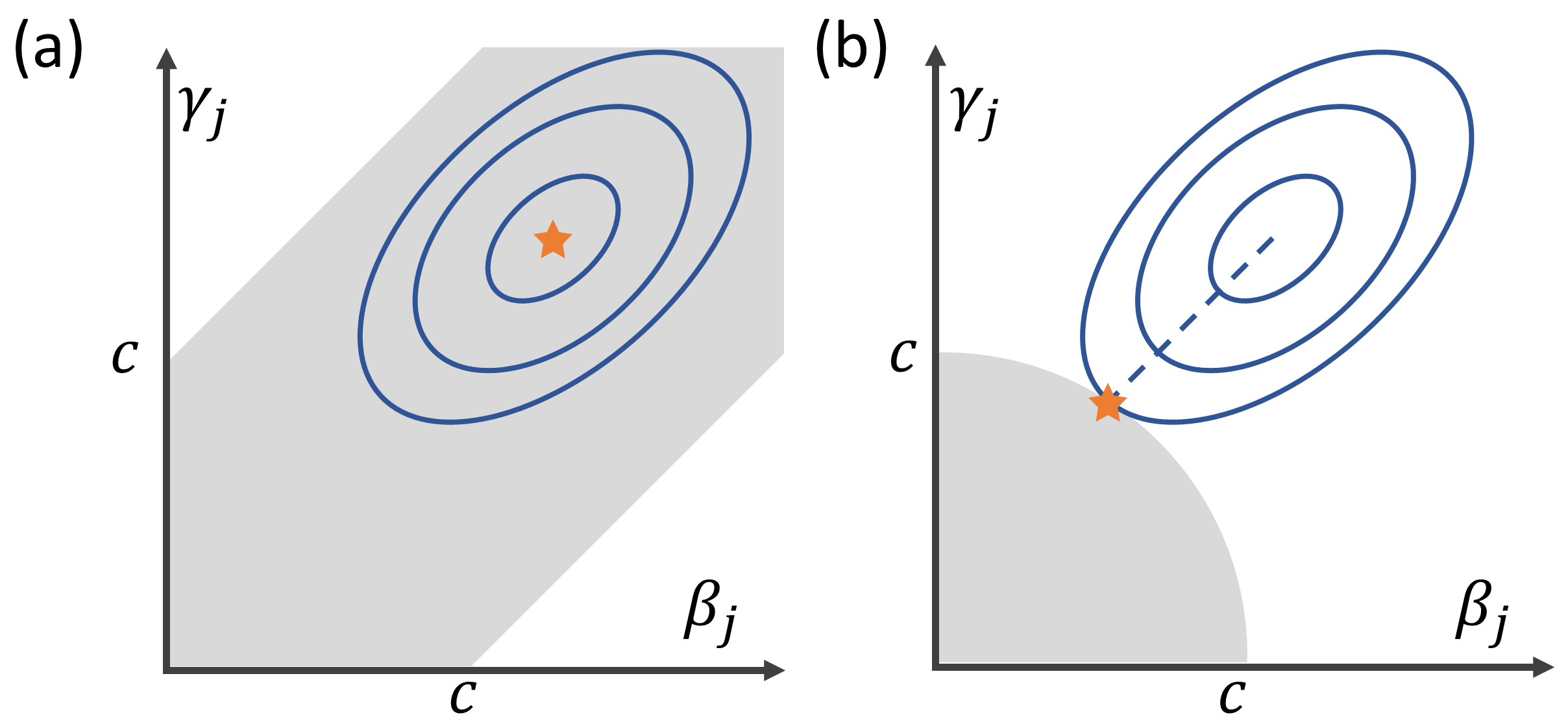
Figure 1: Illustrations for the structural sparse penalties and the optimal solution regarding the regression coefficients of $X_{j}$. Figure 1(a) shows the inequality constraint of fused lasso-type (gray shading; $|\beta_{j}-\gamma_{j}|\leq c$) and the log-likelihood function (blue contour lines), while Figure 1(b) shows the inequality constraint of group lasso-type (gray shading; $\sqrt{\beta_{j}^{2}+\gamma^{2}_{j}}\leq c$) and the log-likelihood function. The star marks indicate the points of the optimal solutions. When the unconstrained optimal solutions (center of the contour lines) satisfy $\beta_{j}\approx\gamma_{j}$ as these figures, it is understood that the fused lasso-type estimate is not biased, and the group lasso-type estimate is shrunk to the origin.

Since the log-likelihood of the screening and severity prediction models and the penalty terms are convex [19, 20, 21], these penalized likelihood functions are also convex. The penalized log-likelihood functions have tuning parameters. They can be selected by standard prediction-based techniques such as cross-validation. In Section 5, we demonstrate parameter tuning of the proposed method by cross-validation using several choices of measures.

4.2 Alternating Direction Method of Multipliers for MtCLM

The Alternating Direction Method of Multipliers (ADMM) is a popular algorithm used for convex optimization problems where the objective function is the sum of two convex functions. ADMM introduces redundant optimization parameters and breaks down the problem into smaller, more tractable components. It is widely applicable to sparse estimation methods, including the fused lasso and the group lasso [16].

To derive the ADMM algorithm for MtCLM, we prepare another expression for the penalties. Let $\boldsymbol{\Theta}=(\boldsymbol{\beta}~{}\boldsymbol{\gamma})$, and the penalty terms are re-expressed as

$$\mathcal{P}_{F}(\boldsymbol{\Theta};\lambda_{F})= ~{}\lambda_{F}\|{\boldsymbol{\Theta}}{\boldsymbol{d}}\|_{1},$$

$$\mathcal{P}_{G}(\boldsymbol{\beta},\boldsymbol{\gamma};\lambda_{F})= ~{}\lambda_{G}\sum_{j=1}^{p}\|{\boldsymbol{\theta}}_{j}\|_{2},$$

where ${\boldsymbol{d}}=(1-1)^{T}$, and ${\boldsymbol{\theta}}_{j}~{}(j=1,\ldots,p)$ are row vectors of $\boldsymbol{\Theta}$. The fused-lasso penalty can be expressed as a special case of the generalized lasso [22], but we write as above for convenience.

Now we derive the ADMM algorithm for the problem (11). The optimization problem (11) is equivalent to the following one, which introduces redundant parameters ${\boldsymbol{a}}\in\mathbb{R}^{p}$ and ${\bf B}=({\boldsymbol{b}}_{\cdot 1}~{}{\boldsymbol{b}}_{\cdot 2})\in\mathbb{R}^{p\times 2}$:

$$\begin{array}[]{c}\displaystyle\min_{\alpha,\boldsymbol{\zeta},\boldsymbol{\Theta},{\boldsymbol{a}},{\bf B}}~{}-\frac{1}{n}\ell(\mathbf{Y},\mathbf{X},\alpha,\boldsymbol{\zeta},\boldsymbol{\Theta},{\bf B})+\lambda_{F}\|{\boldsymbol{a}}\|_{1}+\lambda_{11}\|{\boldsymbol{b}}_{\cdot 1}\|_{1}+\lambda_{12}\|{\boldsymbol{b}}_{\cdot 2}\|_{1}\\ \text{subject to}~{}~{}~{}\boldsymbol{\Theta}{\boldsymbol{d}}={\boldsymbol{a}},\boldsymbol{\Theta}=\mathbf{B}.\end{array}$$ (15)

The augmented Lagrangian of this problem is defined as

$$L(\alpha,\boldsymbol{\zeta},\boldsymbol{\Theta},{\boldsymbol{a}},{\bf B})= ~{}-\frac{1}{n}\ell(\mathbf{Y},\mathbf{X},\alpha,\boldsymbol{\zeta},\boldsymbol{\Theta},{\bf B})+\lambda_{F}\|{\boldsymbol{a}}\|_{1}+{\boldsymbol{u}}^{T}(\boldsymbol{\Theta}{\boldsymbol{d}}-{\boldsymbol{a}})+\frac{\mu_{F}}{2}\|\boldsymbol{\Theta}{\boldsymbol{d}}-{\boldsymbol{a}}\|^{2}_{2}$$

$$~{}~{}~{}~{}+\lambda_{11}\|{\boldsymbol{b}}_{\cdot 1}\|_{1}+\lambda_{12}\|{\boldsymbol{b}}_{\cdot 2}\|_{1}+\mathrm{tr}\left\{\mathbf{V}^{T}(\boldsymbol{\Theta}-\mathbf{B})\right\}+\frac{\mu_{1}}{2}\|\boldsymbol{\Theta}-\mathbf{B}\|^{2}_{F},$$ (16)

where $\boldsymbol{u}$ and $\mathbf{V}=({\boldsymbol{v}}_{\cdot 1}~{}{\boldsymbol{v}}_{\cdot 2})$ are Lagrange multiliers and $\mu_{F},\mu_{1}$ are tuning parameters for optimization. In ADMM, the parameters are updated in sequence to minimize (16). The Lagrange multipliers are updated by the gradient descent. Given the parameters of the previous step, the updating formulae are given below:

$$(\alpha^{t+1},\boldsymbol{\zeta}^{t+1},\boldsymbol{\Theta}^{t+1})= ~{}\mathop{\rm argmin}\limits_{\boldsymbol{\alpha},\boldsymbol{\zeta},\boldsymbol{\Theta}}~{}L(\alpha,\boldsymbol{\zeta},\boldsymbol{\Theta},{\boldsymbol{a}}^{t},\mathbf{B}^{t}),$$ (17)

$$\boldsymbol{a}^{t+1}= ~{}\mathop{\rm argmin}\limits_{\boldsymbol{a}}~{}\lambda_{F}\|{\boldsymbol{a}}\|_{1}+\boldsymbol{u}^{tT}(\boldsymbol{\Theta}^{t+1}{\boldsymbol{d}}-\boldsymbol{a})+\frac{\mu_{F}}{2}\|\boldsymbol{\Theta}^{t+1}{\boldsymbol{d}}-\boldsymbol{a}\|_{2}^{2},$$ (18)

$$\mathbf{B}^{t+1}= ~{}\mathop{\rm argmin}\limits_{\mathbf{B}}~{}\lambda_{11}\|{\boldsymbol{b}}_{\cdot 1}\|_{1}+\lambda_{12}\|{\boldsymbol{b}}_{\cdot 2}\|_{1}$$

$$~{}~{}~{}~{}~{}~{}~{}~{}~{}~{}~{}~{}+\mathrm{tr}\left\{\mathbf{V}^{tT}(\boldsymbol{\Theta}^{t+1}-\mathbf{B})\right\}+\frac{\mu_{1}}{2}\|\boldsymbol{\Theta}^{t+1}-\mathbf{B}\|^{2}_{2},$$ (19)

$$\boldsymbol{u}^{t+1}= ~{}\boldsymbol{u}^{t}+\rho(\boldsymbol{\Theta}^{t+1}{\boldsymbol{d}}-\boldsymbol{a}^{t+1}),$$ (20)

$$\mathbf{V}^{t+1}= ~{}\mathbf{V}^{t}+\rho(\boldsymbol{\Theta}^{t+1}-\mathbf{B}^{t+1}),$$ (21)

where $\rho$ is a step size for each ADMM iteration. The small problem of (17) does not have an explicit solution, so it must be solved using an iterative algorithm. Since the target function of (17) is convex, it can be solved using an off-the-shelf solver. In our implementation, we used the optim package in R. The problems (18) and (19) have explicit solutions:

$$\boldsymbol{a}^{t+1}= ~{}S(\boldsymbol{\Theta}^{t+1}{\boldsymbol{d}}+\mu_{F}^{-1}\boldsymbol{u}^{t},\mu_{F}^{-1}\lambda_{F}),$$ (22)

$$\mathbf{\boldsymbol{b}}_{\cdot 1}^{t+1}= ~{}S(\boldsymbol{\beta}^{t+1}+\mu_{1}^{-1}{\boldsymbol{v}}_{\cdot 1}^{t+1},\mu_{1}^{-1}\lambda_{11}),$$ (23)

$$\mathbf{\boldsymbol{b}}_{\cdot 2}^{t+1}= ~{}S(\boldsymbol{\gamma}^{t+1}+\mu_{1}^{-1}{\boldsymbol{v}}_{\cdot 2}^{t+1},\mu_{1}^{-1}\lambda_{12}),$$ (24)

where the function $S(z,\xi)=\mathrm{sign}(z)(|z|-\xi)_{+}$ is the soft-thresholding operator, which is applied elementwise to a vector. Repeat steps (17) through (21) until an appropriate convergence criterion is met to obtain the final estimate. The algorithm for (12) is derived in a similar way, which can be found in Appendix B.

5 Numerical Experiments

In this section, to evaluate the performance of the proposed method, we perform numerical experiments in settings with low-dimensional predictors ($X\in\mathbb{R}^{10}$) and high-dimensional predictors ($X\in\mathbb{R}^{500}$). In both settings, the sample size is fixed at $N=200$. Response $Y$ has four levels $\{0,1,2,3\}$, generated through thresholding the latent variable $Y^{*}$ and $Y^{**}$ with independent logistic errors. The covariates are generated from a standard normal distribution independent of each other. We prepared five scenarios which have different generation models:

1. Parallel CLM,

2. MtCLM, whose covariates are only associated with diagnosis,

3. MtCLM, whose two models share the same predictors and the same regression coefficients,

4. MtCLM, whose two models share the same predictors but their regression coefficients have inverse signs,

5. MtCLM, whose two models share only one major predictor with the same regression coefficient.

Details on the generation models are found in Appendix C. Note that Scenario 3 appears to satisfy the parallelism assumption, but not as mentioned in Section 3.2. Scenarios 2 to 5 do not meet the parallelism assumption, and in particular, Scenarios 2 and 4 are in serious violation.

For comparison, we use the following methods and implementations:

• Binomial Logistic Regression (with L1 penalty): glmnet package [13, 23],

• CLM (non-penalized): polr function in R package MASS [24],

• CLM (with L1 penalty): ordinalNet package [12],

• NPCLM (with L2 smoothing): serp package [11, 25],

• NPCLM (with L1 penalty): ordinalNet package [12],

• MtCLM (with L1 penalty): glmnet for screening, ordinalNet for severity prediction,

• MtCLM (with L1 + Fused lasso penalty): our implementation,

• MtCLM (with L1 + Group lasso penalty): our implementation.

These methods, except for polr and serp, have parameters that control the strength of regularization terms like $\lambda_{F}$ and $\lambda_{G}$ in MtCLM. Such parameters of the comparative methods are selected using 5-fold cross-validation (CV) from 4 points (0.005, 0.01, 0.05, 0.1). For the proposed methods, $(\lambda_{11},\lambda_{12})$ are fixed at $(0.01,0.05)$, and $\lambda_{F},\lambda_{G}$ are chosen from 4 points (0.005, 0.01, 0.05, 0.1) using 5-fold CV in the low-dimensional settings; $(\lambda_{11},\lambda_{12})$ are fixed at $(0.05,0.1)$, and $\lambda_{F},\lambda_{G}$ are chosen from 3 points (0.01, 0.05, 0.1) using 5-fold CV in the high-dimensional settings. For the comparative experiment, there are many choices of evaluation measures. We report the area under the receiver operating characteristic curve (ROC-AUC; also referred to as AUC in this paper) and the F1 score for the screening task and report the overall accuracy and mean absolute errors (MAE) for $Y$ for the joint task of screening and severity prediction. Details about the evaluation measure are found in Appendix C. We simulate 1,000 datasets in a low-dimensional setting and 200 datasets in a high-dimensional setting, and the mean and standard deviation (SD) are reported for all measures.

5.1 Appropriate Measure for Cross-validation

Firstly, we assess which measure is appropriate for the cross-validation of the proposed methods. We compare the following measures: log-likelihood, overall accuracy, MAE for $Y$, AUC for screening, and F1 score for screening. As demonstrated in Appendix C, the log-likelihood-based CV produced the least dispersed and/or the best estimates across all evaluation measures. Therefore, we will employ the log-likelihood-based CV for all proposed methods henceforth.

5.2 Low-dimensional Settings

Table 1 shows the main results of comparative experiments on the dataset with $X\in\mathbb{R}^{10}$. On the whole, the proposed methods were competitive with the existing methods in all scenarios. Although Scenario 1 is designed to best fit CLM, the proposed method performed as well as CLM. NPCLM (serp) was not as good as other methods. The generative models for Scenarios 2 through 5 are MtCLM, and Scenarios 2 and 4 highly violate the parallelism assumption of the CLM. In Scenario 2, MtCLM performed as well as the binomial logistic regression in screening while the CLM and NPCLM did not. In this scenario, we do not show the overall accuracy and MAE since severity is designed to be independent of the predictors. In Scenario 3, all models except NPCLM (serp) performed well, and the MtCLM with fused-lasso penalty was slightly better than others in MAE. The reason why the fused lasso-type penalty worked well may be the true parameter vectors of the two models are identical. NPCLM (L1) performed as well as others on average, but F1 and MAE had larger SD. In Scenario 4, only MtCLM performed well in both screening and severity prediction; NPCLM, despite being flexible enough, did not perform well in F1, Accuracy, and MAE. In Scenario 5, we obtained a similar result as Scenario 3, possibly due to the lead predictor in Scenario 5 being the same as Scenario 3.

The performance indices concerning variable selection for MtCLM are also provided in Appendix D. The L1 + fused lasso-type penalty tended to yield high sensitivity but low specificity results, while the L1 + group lasso-type penalty and the L1 penalty generally produced results with higher specificity. Both MtCLM (L1) and MtCLM (L1 + Group) exhibited competitive performance in terms of the F1 score.

Table 1: Comparative analysis of the predictive performance measures between MtCLM and other methods low-dimensional settings ($N=200,p=10$). MtCLM is the proposed model. “L1”, “Fused”, and “Group” denote the types of penalty terms used in each method. The means and standard deviations were calculated from the 1,000 repetitions.

Mean (SD)
	Screening (binary)		Overall (four levels)
Method	AUC	F1	Accuracy	MAE
Scenario 1
Binom. Logistic Reg. (L1)	.913 (.0041)	.827 (.0076)	-	-
CLM (non-penalized)	.913 (.0035)	.830 (.0054)	.653 (.0065)	.447 (.0171)
CLM (L1)	.915 (.0029)	.828 (.0086)	.655 (.0062)	.450 (.0209)
NPCLM (serp)	.907 (.0060)	.805 (.0074)	.629 (.0039)	.554 (.0165)
NPCLM (L1)	.916 (.0028)	.823 (.0125)	.654 (.0081)	.463 (.0286)
MtCLM (L1)	.913 (.0041)	.827 (.0075)	.642 (.0098)	.449 (.0200)
MtCLM (L1 + Fused)	.916 (.0033)	.831 (.0072)	.646 (.0099)	.443 (.0204)
MtCLM (L1 + Group)	.915 (.0036)	.830 (.0073)	.643 (.0099)	.450 (.0212)
Scenario 2
Binom. Logistic Reg. (L1)	.914 (.0039)	.828 (.0072)	-	-
CLM (non-penalized)	.901 (.0090)	.790 (.0164)	-	-
CLM (L1)	.912 (.0069)	.771 (.0206)	-	-
NPCLM (serp)	.907 (.0060)	.796 (.0101)	-	-
NPCLM (L1)	.914 (.0019)	.744 (.0263)	-	-
MtCLM (L1)	.914 (.0039)	.828 (.0072)	-	-
MtCLM (L1 + Fused)	.915 (.0034)	.830 (.0068)	-	-
MtCLM (L1 + Group)	.915 (.0034)	.830 (.0068)	-	-
Scenario 3
Binom. Logistic Reg. (L1)	.915 (.0042)	.828 (.0077)	-	-
CLM (non-penalized)	.915 (.0031)	.832 (.0049)	.660 (.0070)	.414 (.0140)
CLM (L1)	.918 (.0026)	.832 (.0066)	.663 (.0069)	.415 (.0178)
NPCLM (serp)	.909 (.0059)	.806 (.0072)	.633 (.0043)	.529 (.0157)
NPCLM (L1)	.918 (.0029)	.828 (.0109)	.662 (.0092)	.427 (.0269)
MtCLM (L1)	.915 (.0042)	.828 (.0078)	.655 (.0087)	.414 (.0143)
MtCLM (L1 + Fused)	.918 (.0030)	.832 (.0072)	.658 (.0087)	.410 (.0160)
MtCLM (L1 + Group)	.916 (.0036)	.830 (.0073)	.655 (.0090)	.417 (.0164)
Scenario 4
Binom. Logistic Reg. (L1)	.914 (.0040)	.827 (.0072)	-	-
CLM (non-penalized)	.870 (.0176)	.776 (.0137)	.566 (.0060)	.727 (.0352)
CLM (L1)	.895 (.0197)	.766 (.0179)	.563 (.0092)	.772 (.0518)
NPCLM (serp)	.908 (.0061)	.800 (.0088)	.641 (.0121)	.635 (.0227)
NPCLM (L1)	.917 (.0043)	.717 (.0251)	.545 (.0244)	.894 (.0617)
MtCLM (L1)	.914 (.0040)	.827 (.0072)	.700 (.0077)	.501 (.0142)
MtCLM (L1 + Fused)	.915 (.0037)	.829 (.0070)	.702 (.0075)	.498 (.0139)
MtCLM (L1 + Group)	.916 (.0036)	.829 (.0070)	.702 (.0075)	.496 (.0137)
Scenario 5
Binom. Logistic Reg. (L1)	.914 (.0044)	.830 (.0074)	-	-
CLM (non-penalized)	.912 (.0040)	.830 (.0053)	.658 (.0072)	.420 (.0146)
CLM (L1)	.914 (.0030)	.830 (.0072)	.661 (.0072)	.422 (.0179)
NPCLM (serp)	.908 (.0061)	.807 (.0076)	.637 (.0050)	.525 (.0164)
NPCLM (L1)	.916 (.0028)	.826 (.0113)	.662 (.0089)	.433 (.0266)
MtCLM (L1)	.914 (.0043)	.830 (.0074)	.662 (.0089)	.411 (.0143)
MtCLM (L1 + Fused)	.915 (.0035)	.831 (.0068)	.662 (.0086)	.412 (.0154)
MtCLM (L1 + Group)	.916 (.0037)	.832 (.0069)	.662 (.0092)	.413 (.0160)

5.3 High-dimensional Settings

Assuming high-dimensional data such as RNA microarray data, we conduct comparative experiments on high-dimensional datasets. The sample size is fixed at $N=200$ and the dimension of $X$ is set to be $500$. The NPCLM models are not included in this experiment because they demonstrated relatively poor performance in low-dimensional settings. Additionally, the non-penalized CLM is also excluded.

The results are presented in Table 2. For the high-dimensional datasets, MtCLM with structured penalties demonstrated superior performance in many scenarios and measures. CLM (L1) exhibited similar behavior to that in the low-dimensional settings, namely, it performed well in Scenarios 1, 3, and 5, but not in Scenarios 2 and 4. MtCLM with the fused-lasso penalty performed relatively well in Scenario 3, which was the same in the low-dimensional settings. MtCLM with the group-lasso penalty showed superior performance in many settings, and it had the smallest variance in AUC across all scenarios. The performance of variable selection is also reported in Appendix D. MtCLM with the L1 + group lasso-type penalty achieved the best F1 score, primarily due to its high specificity.

Table 2: Comparative analysis of the predictive performance measures between MtCLM and other methods high-dimensional settings ($N=200,p=500$). MtCLM is the proposed model. “L1”, “Fused”, and “Group” denote the types of penalty terms used in each method. The means and standard deviations were calculated from the 200 repetitions.

Mean (SD)
	Screening (binary)		Overall (four levels)
Method	AUC	F1	Accuracy	MAE
Scenario 1
Binom. Logistic Reg. (L1)	.908 (.0099)	.821 (.0118)	-	-
CLM (L1)	.911 (.0038)	.816 (.0133)	.643 (.0080)	.478 (.0279)
MtCLM (L1)	.908 (.0088)	.821 (.0110)	.627 (.0139)	.478 (.0220)
MtCLM (L1 + Fused)	.913 (.0026)	.826 (.0076)	.635 (.0127)	.463 (.0224)
MtCLM (L1 + Group)	.913 (.0015)	.825 (.0094)	.625 (.0190)	.485 (.0319)
Scenario 2
Binom. Logistic Reg. (L1)	.908 (.0080)	.820 (.0107)	-	-
CLM (L1)	.909 (.0116)	.745 (.0221)	-	-
MtCLM (L1)	.908 (.0075)	.820 (.0103)	-	-
MtCLM (L1 + Fused)	.910 (.0034)	.821 (.0125)	-	-
MtCLM (L1 + Group)	.913 (.0018)	.824 (.0115)	-	-
Scenario 3
Binom. Logistic Reg. (L1)	.909 (.0068)	.822 (.0099)	-	-
CLM (L1)	.912 (.0037)	.822 (.0106)	.653 (.0105)	.440 (.0263)
MtCLM (L1)	.909 (.0078)	.821 (.0112)	.644 (.0118)	.437 (.0196)
MtCLM (L1 + Fused)	.914 (.0025)	.827 (.0076)	.650 (.0115)	.427 (.0212)
MtCLM (L1 + Group)	.914 (.0016)	.825 (.0093)	.641 (.0164)	.444 (.0311)
Scenario 4
Binom. Logistic Reg. (L1)	.907 (.0099)	.820 (.0135)	-	-
CLM (L1)	.904 (.0184)	.743 (.0223)	.546 (.0116)	.844 (.0542)
MtCLM (L1)	.908 (.0077)	.821 (.0113)	.689 (.0124)	.518 (.0229)
MtCLM (L1 + Fused)	.911 (.0048)	.821 (.0140)	.689 (.0174)	.517 (.0282)
MtCLM (L1 + Group)	.915 (.0032)	.826 (.0129)	.694 (.0137)	.508 (.0252)
Scenario 5
Binom. Logistic Reg. (L1)	.908 (.0063)	.820 (.0099)	-	-
CLM (L1)	.908 (.0042)	.818 (.0118)	.650 (.0103)	.448 (.0287)
MtCLM (L1)	.907 (.0086)	.819 (.0120)	.645 (.0116)	.436 (.0198)
MtCLM (L1 + Fused)	.912 (.0018)	.824 (.0072)	.650 (.0098)	.426 (.0189)
MtCLM (L1 + Group)	.912 (.0017)	.823 (.0107)	.642 (.0151)	.439 (.0276)

6 Real Data Analysis and Parameter Interpretation

In this section, we report the results of applying the proposed methods and some existing methods.

Debernardi et al. (2020) provide an open and cleaned dataset on the concentration of certain proteins in the urine of healthy individuals and patients with pancreatic ductal adenocarcinoma (PDAC) or benign hepatobiliary diseases [26]. The dataset was downloaded from Kaggle datasets on July 3rd, 2023 . The Debernardi dataset consists of 590 individuals and includes the concentration of five molecules (creatinine, LYVE1, REG1B, TFF1, REG1A), cancer diagnosis, cancer stage, and certain demographic factors. They reported that a combination of the three molecules, LYVE1, REG1B, and TFF1, showed good predictive performance in detecting PDAC. To accommodate the composite task of screening and severity prediction, we defined the response variable as follows:

• 0 represents no PDAC, corresponding to "diagnosis" being equal to 1 or 2 in the original dataset.

• 1 represents PDAC at stages I, IA, and IB.

• 2 represents PDAC at stages II, IIA, and IIB.

• 3 represents PDAC at stage III.

• 4 represents PDAC at stage IV.

In the original dataset, individuals with $diagnosis=2$ have benign hepatobiliary diseases but do not have cancer. Therefore, individuals in the original dataset with $diagnosis\in\{1,2\}$ are redefined as 0. The composite response is summarized in Table 3. For further descriptive information on the dataset, refer to Appendix E.

Table 3: Summary for the composite response

Response Levels	0	1	2	3	4
# of Cases	391	16	86	76	21

We applied the methods CLM (polr), CLM (L1), MtCLM (L1), MtCLM (L1 + Fused), and MtCLM (L1 + Group) to this composite response, using age and the concentrations of molecules as predictors. Note that REG1A was excluded from the analysis due to the presence of missing values in about half of the cases. For the methods with tuning parameters, we selected them using 5-fold cross-validation.

Table 4 shows the estimated regression coefficients of these methods.

Table 4: Estimated regression coefficients for each model. CLM is a conventional ordinal regression model, and MtCLM is the proposed one. L1, Fused, and Group denote the types of regularization terms. The hyphen indicates that the regression coefficient is zero, in other words, the variable is not selected.

Model	Regularization	Task	age	creatinine	LYVE1	REG1B	TFF1
CLM	None	Overall	0.634	$-0.286$	2.381	0.474	0.023
	L1	Overall	0.594	$-0.169$	1.847	0.471	-
MtCLM	L1	Screening	0.711	$-0.467$	2.001	0.594	0.113
		Sev. Pred.	-	0.259	-	-	-
	L1 + Fused	Screening	0.677	$-0.376$	1.761	0.582	0.066
		Sev. Pred.	-	0.241	-	-	-
	L1 + Group	Screening	0.680	$-0.377$	1.666	0.592	0.089
		Sev. Pred.	-	0.249	-	-	-

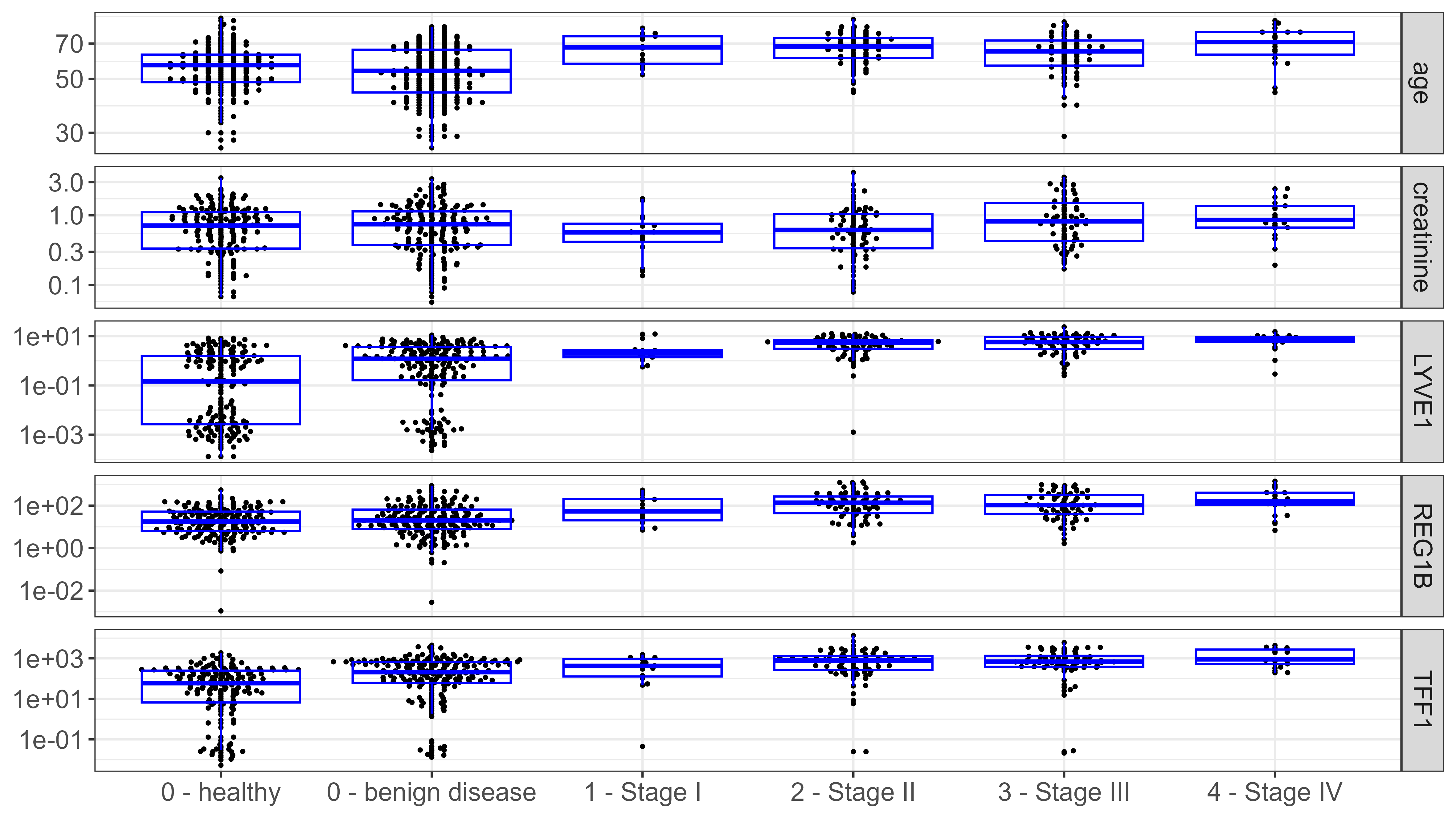
Figure A3: A box plot overlaid by beeswarm. This shows univariate relationships between markers and severity in the dataset provided by Debernardi et al. (2020).

The coefficients of CLM (polr) and CLM (L1) indicated that age, LYVE1, and REG1B were positively associated with the composite response, and that creatinine was negatively associated. On the other hand, the coefficients of the MtCLMs suggested that creatinine was negatively associated with the presence of cancer but positively associated with cancer severity. These inverse relationships can also be observed by the descriptive analysis (see Figure A3). More importantly, while the three molecules were associated with the outcome in the screening model, they showed no association with the cancer severity. Additionally, creatinine has been reported to have a negative association with the presence of pancreatic cancer [27, 28]. Our results by MtCLM are consistent with these findings, although it should be noted that these results were about serum creatinine. The association of REG1B with cancer severity disappeared when using the fused and group lasso regularizations. These results suggest that the two tasks, screening and severity prediction, had significantly different structures in Debernardi’s dataset, making MtCLM a more suitable choice.

In interpreting these results, it is important to note that our defined category $Y=0$ includes not only healthy individuals but also cases of non-cancer diseases. As shown in Appendix E, there are differences in the distribution of markers between healthy individuals and those with non-cancer diseases.

7 Discussion

In this study, we have discussed the combined problem of screening and severity prediction, considering that some biomarkers are associated not only with the presence of disease but also with disease severity. To address this problem, we have proposed a multi-task approach with structured sparse regularization, MtCLM, leveraging the shared structure between the two tasks. MtCLM is an ordinal regression model, which is more flexible than CLM, but unlike NPCLM, it is valid across the entire predictor space and interpretable. The performance of MtCLM on prediction and variable selection was verified by simulation, and an example of real data analysis was provided.

This study suggests the usefulness of a multi-task learning approach for tasks that are expected to have shared structures in medicine, such as screening and severity prediction of the same disease. The idea of multi-task learning is not considered to be prevalent in the field of biomedical research. However, many diseases share risk factors and genetic abnormalities (e.g., hyperlipemia is a risk factor for cardiovascular and cerebrovascular diseases (e.g., [29]), and the HER2 gene is amplified in ovarian and gastric cancers in addition to breast cancer (e.g., [30])), and the idea of multi-task learning that takes advantage of commonalities among tasks may be useful in building prediction models or investigating prognostic factors using limited data.

Appendix Appendix A Further Illustrations for the Learning with Structural Sparse Regularization

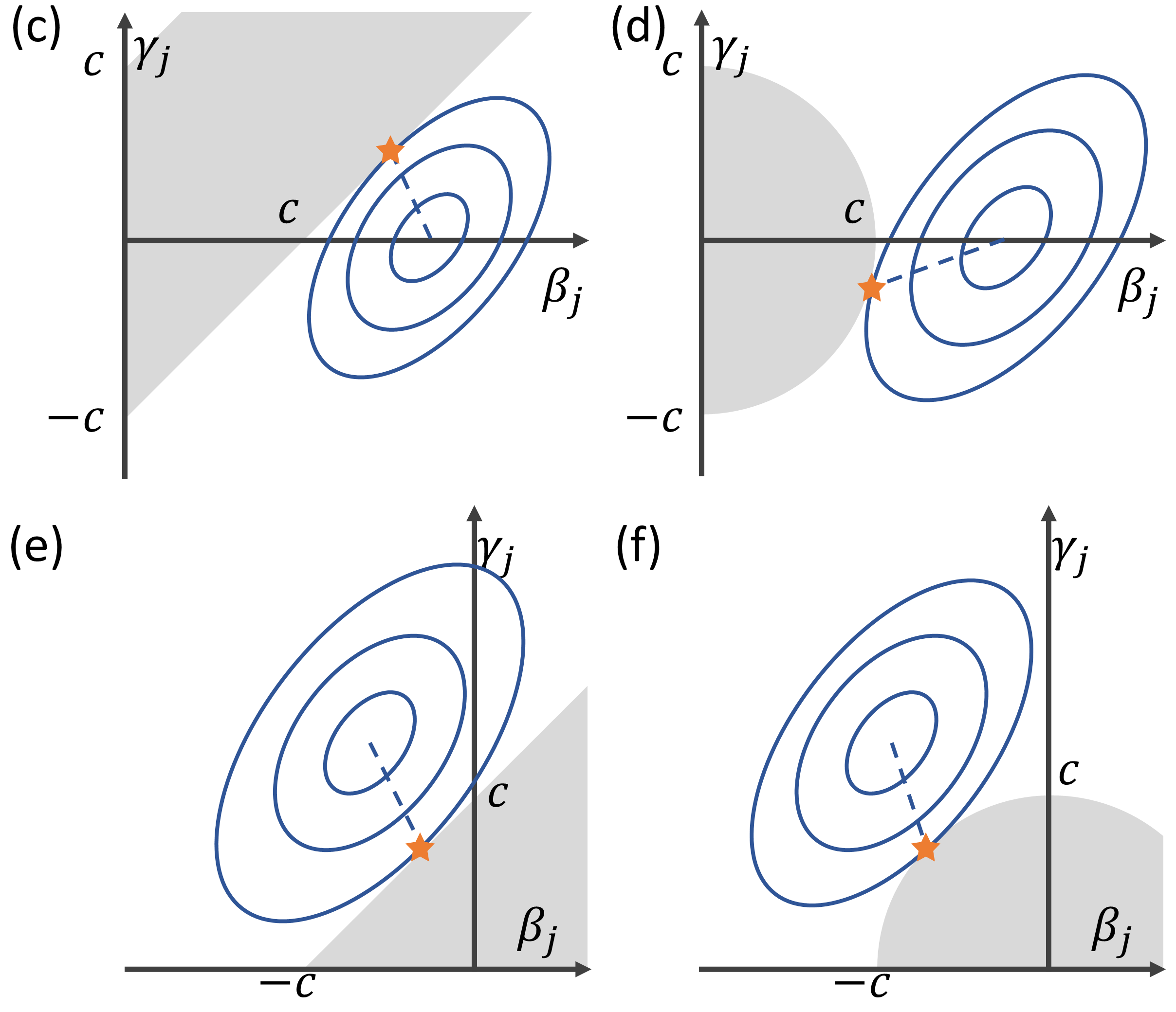
Figure A1: (Continues from Figure 1) Illustrations for the structural sparse penalties and the optimal solution regarding the regression coefficients of $X_{j}$. (Left) the inequality constraint of fused lasso-type (gray shading; $|\beta_{j}-\gamma_{j}|\leq c$) and the log-likelihood function (blue contour lines). (Right) the inequality constraint of group lasso-type (gray shading; $\sqrt{\beta_{j}^{2}+\gamma^{2}_{j}}\leq c$) and the log-likelihood function. (Upper) the cases with $\beta_{j}>0$ and $\gamma_{j}=0$ being true. (Lower) the cases with $\beta_{j}>0$ and $\gamma_{j}<0$ being true. The star marks indicate the points of the optimal solutions.

Appendix Appendix B Details of ADMM Algorithm

Appendix B.1 ADMM for Group lasso-type Estimation

In this subsection, we derive the ADMM algorithm for the problem (12). The optimization problem (12) is equivalent to the following problem, which introduces a redundant parameter ${\bf B}\in\mathbb{R}^{p\times 2}$.

$$\begin{array}[]{c}\displaystyle\min_{\alpha,\boldsymbol{\zeta},\boldsymbol{\Theta},{\boldsymbol{B}}}~{}-\frac{1}{n}\ell(\mathbf{Y},\mathbf{X},\alpha,\boldsymbol{\zeta},\boldsymbol{\Theta})+\lambda_{G}\sum_{j=1}^{p}\|{\boldsymbol{b}}_{j\cdot}\|_{2}+\lambda_{11}\|{\boldsymbol{b}}_{\cdot 1}\|_{1}+\lambda_{12}\|{\boldsymbol{b}}_{\cdot 2}\|_{1}\\ \text{subject to}~{}~{}~{}\boldsymbol{\Theta}={\bf B},\end{array}$$ (A3)

where ${\boldsymbol{b}}_{j\cdot}~{}(j=1,\ldots,p)$ are row vectors of ${\bf B}$. The augmented Lagrangian of this problem is defined as

$$L(\alpha,\boldsymbol{\zeta},\boldsymbol{\Theta},{\bf B})= ~{}-\frac{1}{n}\ell(\mathbf{Y},\mathbf{X},\alpha,\boldsymbol{\zeta},\boldsymbol{\Theta})+\lambda_{G}\sum_{j=1}^{p}\|{\boldsymbol{b}}_{j\cdot}\|_{2}+\lambda_{11}\|{\boldsymbol{b}}_{\cdot 1}\|_{1}+\lambda_{12}\|{\boldsymbol{b}}_{\cdot 2}\|_{1}$$

$$~{}~{}~{}~{}+\mathrm{tr}\{{\bf V}^{T}(\boldsymbol{\Theta}-{\bf B})\}+\frac{\mu}{2}\|\boldsymbol{\Theta}-{\bf B}\|^{2}_{F},$$ (A4)

where $\bf V$ is a Lagrange multilier and $\mu$ is a tuning parameter for optimization. In ADMM, the parameters are updated in sequence to minimize (A4). The Lagrange multipliers are updated by the gradient descent. Given the parameters of the previous step, the updating formulae are given below:

$$(\alpha^{t+1},\boldsymbol{\zeta}^{t+1},\boldsymbol{\Theta}^{t+1})= ~{}\mathop{\rm argmin}\limits_{\boldsymbol{\alpha},\boldsymbol{\zeta},\boldsymbol{\Theta}}~{}L(\alpha,\boldsymbol{\zeta},\boldsymbol{\Theta},{\bf B}^{t}),$$ (A5)

$${\bf B}^{t+1}= ~{}\mathop{\rm argmin}\limits_{\bf B}~{}\lambda_{G}\sum_{j=1}^{p}\|{\boldsymbol{b}}_{j\cdot}\|_{2}+\lambda_{11}\|{\boldsymbol{b}}_{\cdot 1}\|_{1}+\lambda_{12}\|{\boldsymbol{b}}_{\cdot 2}\|_{1}$$

$$~{}~{}~{}~{}+\mathrm{tr}\{{\bf V}^{tT}(\boldsymbol{\Theta}^{t+1}-{\bf B})\}+\frac{\mu}{2}\|\boldsymbol{\Theta}^{t+1}-{\bf B}\|_{F}^{2},$$ (A6)

$${\bf V}^{t+1}= ~{}{\bf V}^{t}+\rho(\boldsymbol{\Theta}^{t+1}-{\bf B}^{t+1}),$$ (A7)

The small problem (A5) does not have an explicit solution, so it has to be solved by an iterative algorithm. Since the target function of (A5) is convex, it can be solved using an off-the-shelf solver. The problems (A6) can be solved in the following 2-step procedure [31, 32]:

$${\boldsymbol{b}}_{\cdot 1}^{{\dagger}}= ~{}S({\boldsymbol{\beta}}^{t+1}+\mu^{-1}{\boldsymbol{v}}_{\cdot 1}^{t},\mu^{-1}\lambda_{11}),$$

$${\boldsymbol{b}}_{\cdot 2}^{{\dagger}}= ~{}S({\boldsymbol{\gamma}}^{t+1}+\mu^{-1}{\boldsymbol{v}}_{\cdot 2}^{t},\mu^{-1}\lambda_{12}),$$

and

$${\boldsymbol{b}}_{j\cdot}^{t+1}= ~{}S_{G}({\boldsymbol{b}}_{j\cdot}^{{\dagger}},\sqrt{2}\mu^{-1}\lambda_{G})~{}~{}~{}(j=1,\ldots,p),$$

where $S_{G}(\boldsymbol{z},\xi)=(1-\frac{\xi}{\|\boldsymbol{z}\|_{2}})_{+}{\boldsymbol{z}}$ is the soft-thresholding operator for a group lasso-type penalty, and ${\boldsymbol{b}}_{j\cdot}^{{\dagger}}$ is the $j$th row vector of ${\mathbf{B}}^{{\dagger}}$. Repeat steps (A5) through (A7) until an appropriate convergence criterion is met to obtain the final estimate.

Appendix B.2 Gradient of the Augmented Langrangian

We derive the gradient of the augmented Lagrangian for the fused lasso-type problem. Note that the derivative of $\sigma(u)$ is $\sigma^{[1]}(u)=\sigma(u)\{1-\sigma(u)\}$, which is also the density function of the logistic distribution. Each gradient is given as follows:

$$\frac{\partial L}{\partial\alpha}=-\frac{1}{n}\frac{\partial\ell}{\partial\alpha}=-\frac{1}{n}\frac{\partial\log\mathcal{L}_{1}}{\partial\alpha}=-\frac{1}{n}\sum_{i=1}^{n}\left[{\bf 1}(Y_{i}=0)-\sigma\{\alpha+X_{i}\boldsymbol{\beta}\}\right],$$

$$\frac{\partial L}{\partial\boldsymbol{\beta}}= ~{}-\frac{1}{n}\frac{\partial}{\partial\boldsymbol{\beta}}\left\{\log\mathcal{L}_{1}+{\boldsymbol{u}}^{T}(\boldsymbol{\Theta}{\boldsymbol{d}}-\boldsymbol{a})+\frac{\mu_{F}}{2}\|\boldsymbol{\Theta}{\boldsymbol{d}}-\boldsymbol{a}\|^{2}_{2}+\mathrm{tr}\left\{\mathbf{V}^{T}(\boldsymbol{\Theta}-\mathbf{B})\right\}+\frac{\mu_{1}}{2}\|\boldsymbol{\Theta}-\mathbf{B}\|^{2}_{F}\right\}$$

$$= ~{}-\frac{1}{n}\sum_{i=1}^{n}\left[{\bf 1}(Y_{i}=0)-\sigma\{\alpha+X_{i}\boldsymbol{\beta}\}\right]X_{i}+{\boldsymbol{u}}+\mu_{F}(\boldsymbol{\Theta}{\boldsymbol{d}}-{\boldsymbol{a}})+{\boldsymbol{v}}_{1}+\mu_{1}({\boldsymbol{\beta}}-{\boldsymbol{b}}_{\cdot 1}),$$

$$\frac{\partial L}{\partial\zeta_{k}}= ~{}-\frac{1}{n}\frac{\partial\log\mathcal{L}_{2}}{\partial\zeta_{k}}$$

$$= ~{}-\frac{1}{n}\sum_{i=1}^{n}\left[\frac{{\bf 1}(Y_{i}=k)\sigma^{[1]}(\zeta_{k}+X_{i}^{T}\boldsymbol{\gamma})}{\sigma(\zeta_{k}+X_{i}^{T}\boldsymbol{\gamma})-\sigma(\zeta_{k-1}+X_{i}^{T}\boldsymbol{\gamma})}-\frac{{\bf 1}(Y_{i}=k+1)\sigma^{[1]}(\zeta_{k}+X_{i}^{T}\boldsymbol{\gamma})}{\sigma(\zeta_{k+1}+X_{i}^{T}\boldsymbol{\gamma})-\sigma(\zeta_{k}+X_{i}^{T}\boldsymbol{\gamma})}\right],$$

$$\frac{\partial L}{\partial\boldsymbol{\gamma}}= ~{}-\frac{1}{n}\frac{\partial}{\partial\boldsymbol{\gamma}}\left\{\log\mathcal{L}_{2}+{\boldsymbol{u}}^{T}(\boldsymbol{\Theta}{\boldsymbol{d}}-\boldsymbol{a})+\frac{\mu}{2}\|\boldsymbol{\Theta}{\boldsymbol{d}}-\boldsymbol{a}\|^{2}_{2}+\mathrm{tr}\left\{\mathbf{V}^{T}(\boldsymbol{\Theta}-\mathbf{B})\right\}+\frac{\mu_{1}}{2}\|\boldsymbol{\Theta}-\mathbf{B}\|^{2}_{F}\right\}$$

$$= ~{}-\frac{1}{n}\sum_{i=1}^{n}\sum_{k=1}^{K}\left[{\bf 1}(Y_{i}=k)X_{i}\frac{\sigma^{[1]}(\zeta_{k}+X_{i}^{T}\boldsymbol{\gamma})-\sigma^{[1]}(\zeta_{k-1}+X_{i}^{T}\boldsymbol{\gamma})}{\sigma(\zeta_{k}+X_{i}^{T}\boldsymbol{\gamma})-\sigma(\zeta_{k-1}+X_{i}^{T}\boldsymbol{\gamma})}\right]$$

$$~{}~{}~{}~{}~{}-{\boldsymbol{u}}-\mu(\boldsymbol{\Theta}{\boldsymbol{d}}-{\boldsymbol{a}})+{\boldsymbol{v}}_{2}+\mu_{1}({\boldsymbol{\gamma}}-{\boldsymbol{b}}_{\cdot 2}).$$

Since $\zeta_{0}=-\infty$ and $\zeta_{K}=\infty$, we have $\sigma^{[1]}(\zeta_{0}+X_{i}^{T}\boldsymbol{\gamma})=\sigma^{[1]}(\zeta_{K}+X_{i}^{T}\boldsymbol{\gamma})=0$.

For the group lasso-type augmented Lagrangian, some modifications are needed. Let $\boldsymbol{v}_{1}$ and $\boldsymbol{v}_{2}$ be the column vectors of $\mathbf{V}$, and then the gradients are

$$\frac{\partial L}{\partial\boldsymbol{\beta}}= ~{}-\frac{1}{n}\frac{\partial}{\partial\boldsymbol{\beta}}\left\{\log\mathcal{L}_{1}+\mathrm{tr}\left\{\mathbf{V}^{T}(\boldsymbol{\Theta}-\mathbf{B})\right\}+\frac{\mu}{2}\|\boldsymbol{\Theta}-\mathbf{B}\|^{2}_{F}\right\}$$

$$= ~{}-\frac{1}{n}\sum_{i=1}^{n}\left[{\bf 1}(Y_{i}=0)-\sigma\{\alpha+X_{i}\boldsymbol{\beta}\}\right]X_{i}+{\boldsymbol{v}}_{1}+\mu(\boldsymbol{\beta}-{\boldsymbol{b}}_{\cdot 1}),$$

$$\frac{\partial L}{\partial\boldsymbol{\gamma}}= ~{}-\frac{1}{n}\frac{\partial}{\partial\boldsymbol{\gamma}}\left\{\log\mathcal{L}_{2}+\mathrm{tr}\left\{\mathbf{V}^{T}(\boldsymbol{\Theta}-\mathbf{B})\right\}+\frac{\mu}{2}\|\boldsymbol{\Theta}-\mathbf{B}\|^{2}_{F}\right\}$$

$$= ~{}-\frac{1}{n}\sum_{i=1}^{n}\sum_{k=1}^{K}\left[{\bf 1}(Y_{i}=k)X_{i}\frac{\sigma^{[1]}(\zeta_{k}+X_{i}^{T}\boldsymbol{\gamma})-\sigma^{[1]}(\zeta_{k-1}+X_{i}^{T}\boldsymbol{\gamma})}{\sigma(\zeta_{k}+X_{i}^{T}\boldsymbol{\gamma})-\sigma(\zeta_{k-1}+X_{i}^{T}\boldsymbol{\gamma})}\right]+{\boldsymbol{v}}_{2}+\mu(\boldsymbol{\gamma}-{\boldsymbol{b}}_{\cdot 2}).$$

Appendix Appendix C Details on the Numerical Experiments

Appendix C.1 Data Generation Models

The datasets for the numerical experiments were generated from the CLM and MtCLM models.

Scenario 1

The generative model is CLM, and the latent variable is defined below:

$$Y^{*}=3X_{1}-0.5X_{2}+\varepsilon,~{}~{}~{}\varepsilon\sim Logistic(0,1).$$

The ordinal response $Y$ is generated by thresholding $Y^{*}$ on its 50, 66.7, and 83.3 percentiles of the population.

Scenario 2

The generative model is MtCLM, and the latent variable is defined below:

$$Y^{*}= ~{}3X_{1}-0.5X_{2}+\varepsilon,~{}~{}~{}\varepsilon\sim Logistic(0,1),$$

$$Y^{**}= ~{}\mathrm{undefined}.$$

The ordinal response $Y$ is set to be zero if $Y^{*}<0$, and for individuals with $Y^{*}\geq 0$, $Y$ is randomly assigned to $\{1,2,3\}$. This implies that the severity prediction task is independent of the predictors.

Scenario 3

The generative model is MtCLM, and the latent variable is defined below:

$$Y^{*}= ~{}3X_{1}-0.5X_{2}+\varepsilon,~{}~{}~{}\varepsilon\sim Logistic(0,1),$$

$$Y^{**}= ~{}3X_{1}-0.5X_{2}+\varepsilon,~{}~{}~{}\varepsilon\sim Logistic(0,1).$$

The ordinal response $Y$ is set to be zero if $Y^{*}<0$, and for individuals with $Y^{*}\geq 0$, $Y$ is assigned to $\{1,2,3\}$ by thresholding $Y^{**}$ on its 33.3 and 66.7 percentiles of the population.

Scenario 4

The generative model is MtCLM, and the latent variable is defined below:

$$Y^{*}= ~{}3X_{1}-0.5X_{2}+\varepsilon,~{}~{}~{}\varepsilon\sim Logistic(0,1),$$

$$Y^{**}= ~{}0.5X_{1}-3X_{2}+\varepsilon,~{}~{}~{}\varepsilon\sim Logistic(0,1).$$

The ordinal response $Y$ is set to be zero if $Y^{*}<0$, and for individuals with $Y^{*}\geq 0$, $Y$ is assigned to $\{1,2,3\}$ by thresholding $Y^{**}$ on its 33.3 and 66.7 percentiles of the population.

Scenario 5

The generative model is MtCLM, and the latent variable is defined below:

$$Y^{*}= ~{}3X_{1}-0.5X_{2}+\varepsilon,~{}~{}~{}\varepsilon\sim Logistic(0,1),$$

$$Y^{**}= ~{}3X_{1}+0.5X_{3}+\varepsilon,~{}~{}~{}\varepsilon\sim Logistic(0,1).$$

The ordinal response $Y$ is set to be zero if $Y^{*}<0$, and for individuals with $Y^{*}\geq 0$, $Y$ is assigned to $\{1,2,3\}$ by thresholding $Y^{**}$ on its 33.3 and 66.7 percentiles of the population.

Appendix C.2 Evaluation Measures

We use the following evaluation measures to evaluate the predictive performance.

• ROC-AUC: the area under the curve for the receiver operating characteristic. We simply refer to it as AUC. This takes values in [0,5, 1.0] and it measures the overall performance for the binary classification of a continuous indicator, taking into account sensitivity and specificity on various cutoff values.

• F1 Score: the harmonic mean of the positive predictive value (PPV, or Precision) and the sensitivity (or Recall), which measures the overall performance for the binary classification of a specific rule.

• Accuracy: the proportion of the accurate prediction across all levels of the ordinal response.

• MAE: the mean absolute error for the ordinal response.

To evaluate the variable selection performance, we use the following measures.

• F1 Score

• False Discovery Rate (FDR): False Positive / Predicted Positive.

• Sensitivity: True Positive / Positive.

• Specificity: True Negative / Negative.

Appendix Appendix D Additional Results for Numerical Experiments

Appendix D.1 CV Measure Selection

Table A1: Predictive performance of MtCLM with various cross-validation measures ($N=200,p=10$). “L1”, “Fused”, and “Group” denote the types of penalty terms. The means and standard deviations were calculated from the 1,000 repetitions.

Mean (SD)
		Screening (binary)		Overall (four levels)
Penalty	CV measure	AUC	F1	Accuracy	MAE
Scenario 1
L1 + Fused	loglike	.916 (.0033)	.831 (.0072)	.646 (.0099)	.443 (.0204)
	AUC	.916 (.0034)	.831 (.0074)	.647 (.0098)	.442 (.0199)
	F1	.916 (.0032)	.831 (.0074)	.646 (.0098)	.443 (.0200)
	Accuracy	.916 (.0033)	.831 (.0074)	.647 (.0099)	.443 (.0203)
	MAE	.916 (.0030)	.831 (.0073)	.647 (.0097)	.442 (.0198)
L1 + Group	loglike	.915 (.0036)	.830 (.0073)	.643 (.0099)	.450 (.0212)
	AUC	.914 (.0031)	.828 (.0080)	.639 (.0127)	.457 (.0269)
	F1	.914 (.0031)	.828 (.0077)	.639 (.0120)	.457 (.0257)
	Accuracy	.914 (.0032)	.829 (.0076)	.640 (.0111)	.455 (.0244)
	MAE	.915 (.0032)	.829 (.0075)	.641 (.0107)	.454 (.0225)
Scenario 2
L1 + Fused	loglike	.915 (.0034)	.830 (.0068)	-	-
	AUC	.915 (.0038)	.828 (.0078)	-	-
	F1	.914 (.0037)	.828 (.0079)	-	-
	Accuracy	.914 (.0040)	.828 (.0081)	-	-
	MAE	.914 (.0043)	.827 (.0094)	-	-
L1 + Group	loglike	.915 (.0034)	.830 (.0068)	-	-
	AUC	.915 (.0029)	.828 (.0082)	-	-
	F1	.915 (.0029)	.829 (.0075)	-	-
	Accuracy	.915 (.0027)	.829 (.0073)	-	-
	MAE	.915 (.0026)	.828 (.0085)	-	-
L1 + Fused	loglike	.918 (.0030)	.832 (.0072)	.658 (.0087)	.410 (.0160)
	AUC	.918 (.0029)	.832 (.0072)	.659 (.0084)	.409 (.0156)
	F1	.918 (.0031)	.831 (.0071)	.658 (.0085)	.410 (.0155)
	Accuracy	.918 (.0031)	.831 (.0072)	.658 (.0086)	.411 (.0157)
	MAE	.918 (.0030)	.831 (.0071)	.658 (.0084)	.410 (.0154)
L1 + Group	loglike	.916 (.0036)	.830 (.0073)	.655 (.0090)	.417 (.0164)
	AUC	.916 (.0031)	.829 (.0084)	.651 (.0119)	.423 (.0215)
	F1	.916 (.0029)	.829 (.0078)	.651 (.0118)	.423 (.0219)
	Accuracy	.916 (.0031)	.829 (.0076)	.652 (.0106)	.422 (.0209)
	MAE	.916 (.0032)	.829 (.0076)	.653 (.0104)	.420 (.0187)
Continued on next page

Table A1: Continued from the previous page.

Mean (SD)
		Screening (binary)		Overall (four levels)
Penalty	CV measure	AUC	F1	Accuracy	MAE
Scenario 4
L1 + Fused	loglike	.915 (.0037)	.829 (.0070)	.702 (.0075)	.498 (.0139)
	AUC	.915 (.0041)	.828 (.0080)	.700 (.0089)	.500 (.0163)
	F1	.914 (.0061)	.827 (.0091)	.699 (.0109)	.502 (.0199)
	Accuracy	.914 (.0050)	.827 (.0084)	.699 (.0099)	.501 (.0184)
	MAE	.914 (.0060)	.827 (.0090)	.699 (.0109)	.502 (.0197)
L1 + Group	loglike	.916 (.0036)	.829 (.0070)	.702 (.0075)	.496 (.0137)
	AUC	.918 (.0033)	.830 (.0087)	.700 (.0110)	.497 (.0180)
	F1	.918 (.0031)	.830 (.0079)	.701 (.0099)	.496 (.0166)
	Accuracy	.918 (.0032)	.830 (.0079)	.702 (.0099)	.496 (.0172)
	MAE	.918 (.0032)	.830 (.0081)	.701 (.0096)	.496 (.0167)
Scenario 5
L1 + Fused	loglike	.915 (.0035)	.831 (.0068)	.662 (.0086)	.412 (.0154)
	AUC	.915 (.0035)	.831 (.0069)	.662 (.0087)	.412 (.0156)
	F1	.915 (.0034)	.831 (.0067)	.661 (.0085)	.412 (.0154)
	Accuracy	.915 (.0034)	.831 (.0066)	.662 (.0086)	.412 (.0154)
	MAE	.915 (.0034)	.831 (.0067)	.661 (.0084)	.412 (.0152)
L1 + Group	loglike	.916 (.0037)	.832 (.0069)	.662 (.0092)	.413 (.0160)
	AUC	.915 (.0031)	.831 (.0075)	.658 (.0117)	.420 (.0211)
	F1	.915 (.0032)	.831 (.0071)	.658 (.0111)	.419 (.0199)
	Accuracy	.915 (.0032)	.831 (.0073)	.659 (.0111)	.418 (.0199)
	MAE	.915 (.0032)	.831 (.0073)	.659 (.0109)	.417 (.0189)

Appendix D.2 Low-dimensional Settings

Table A2: Comparative analysis of the variable selection performance measures between MtCLM and other methods low-dimensional settings ($N=200,p=10$). CLM denotes the conventional cumulative logit model, and MtCLM is the proposed model. “L1”, “Fused”, and “Group” denote the types of penalty terms used in each method. The means and standard deviations were calculated from the 1,000 repetitions.

Mean (SD)
Penalty	F1	FDR	Sensitivity	Specificity
Scenario 2
L1	.437 (.1518)	.672 (.2172)	.922 (.1810)	.699 (.1589)
L1 + Fused	.232 (.0418)	.868 (.0263)	.973 (.1131)	.271 (.1321)
L1 + Group	.381 (.1131)	.746 (.1359)	.948 (.1534)	.628 (.1478)
Scenario 3
L1	.532 (.1189)	.604 (.1559)	.920 (.1275)	.579 (.1932)
L1 + Fused	.474 (.0934)	.683 (.0935)	.998 (.0295)	.411 (.1840)
L1 + Group	.559 (.1067)	.592 (.1151)	.935 (.1206)	.628 (.1367)
Scenario 4
L1	.509 (.1178)	.615 (.1531)	.854 (.1490)	.591 (.1888)
L1 + Fused	.425 (.0628)	.728 (.0534)	.989 (.0524)	.313 (.1508)
L1 + Group	.511 (.1024)	.619 (.1094)	.815 (.1206)	.639 (.1283)
Scenario 5
L1	.533 (.1168)	.605 (.1517)	.922 (.1297)	.581 (.1911)
L1 + Fused	.428 (.0765)	.718 (.0716)	.942 (.1200)	.362 (.1784)
L1 + Group	.557 (.1030)	.594 (.1169)	.941 (.1182)	.621 (.1393)

Appendix D.3 High-imensional Settings

Table A3: Comparative analysis of the variable selection performance measures between MtCLM and other methods high-dimensional settings ($N=200,p=500$). CLM denotes the conventional cumulative logit model, and MtCLM is the proposed model. “L1”, “Fused”, and “Group” denote the types of penalty terms used in each method. The means and standard deviations were calculated from the 200 repetitions.

Mean (SD)
Penalty	F1	FDR	Sensitivity	Specificity
Scenario 2
L1	.083 (.0304)	.956 (.0164)	.740 (.2504)	.966 (.0117)
L1 + Fused	.050 (.0343)	.974 (.0187)	.642 (.2263)	.917 (.0679)
L1 + Group	.387 (.2149)	.563 (.3718)	.573 (.1765)	.993 (.0082)
Scenario 3
L1	.194 (.0584)	.886 (.0378)	.713 (.1619)	.975 (.0118)
L1 + Fused	.229 (.1742)	.856 (.1232)	.866 (.2125)	.928 (.0794)
L1 + Group	.532 (.1804)	.324 (.3647)	.562 (.1296)	.996 (.0059)
Scenario 4
L1	.192 (.0754)	.884 (.0570)	.664 (.1409)	.974 (.0154)
L1 + Fused	.170 (.1112)	.899 (.0779)	.812 (.1085)	.931 (.0716)
L1 + Group	.641 (.2235)	.258 (.3502)	.651 (.1225)	.997 (.0047)
Scenario 5
L1	.193 (.0659)	.888 (.0424)	.739 (.1687)	.974 (.0121)
L1 + Fused	.168 (.1142)	.894 (.0815)	.666 (.1741)	.934 (.0759)
L1 + Group	.550 (.1743)	.295 (.3540)	.562 (.1344)	.996 (.0058)

Appendix Appendix E Further Information of Real Data Analysis

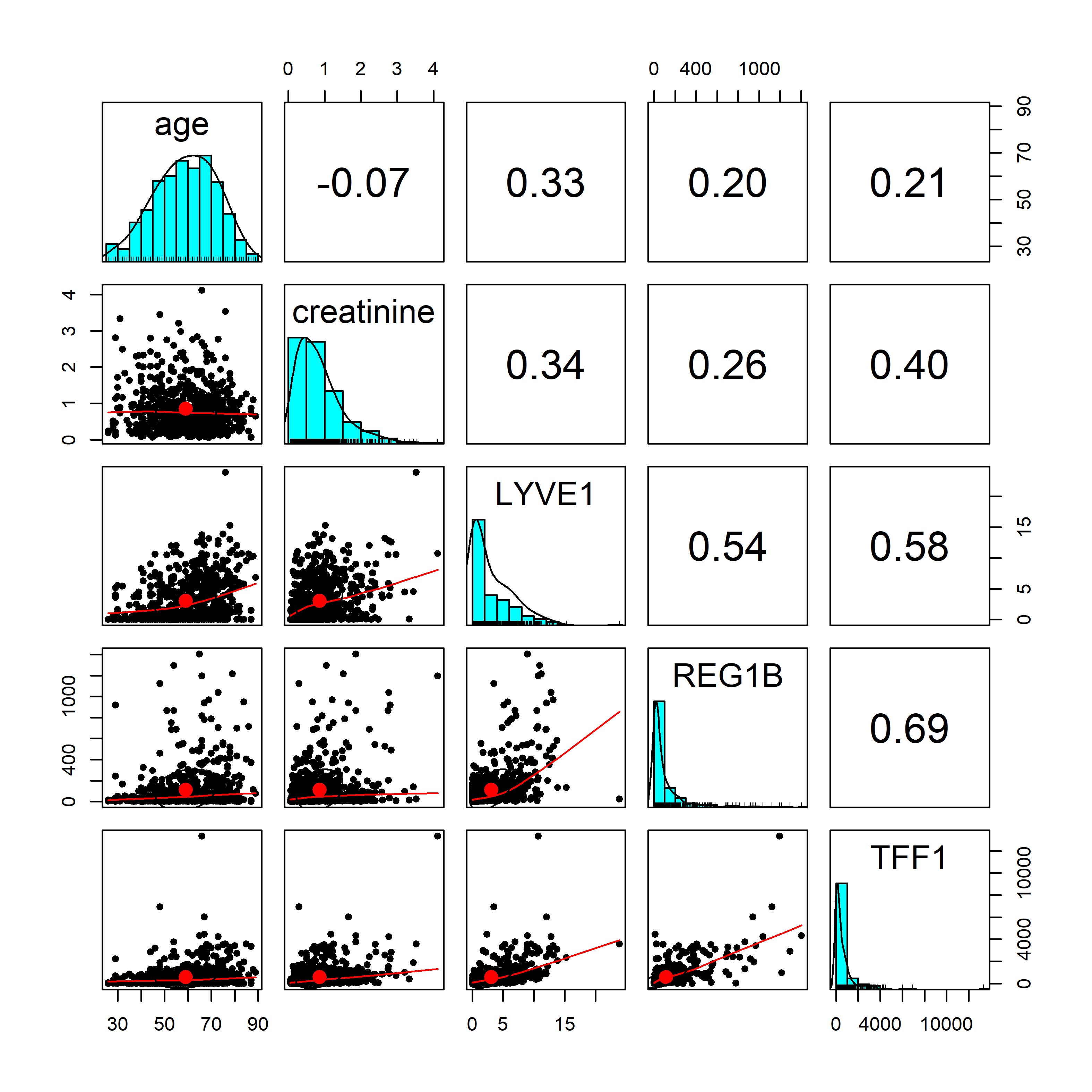
Figure A2: Correlation plot of age and biomarkers in the dataset provided by Debernardi et al. (2020). Each value in the upper-right boxes is Pearson’s correlation.

References

- [1] Biomarkers Definitions Working Group. Biomarkers and surrogate endpoints: preferred definitions and conceptual framework. Clin. Pharmacol. Ther., 69(3):89–95, March 2001.
- [2] Hans Lilja, David Ulmert, and Andrew J Vickers. Prostate-specific antigen and prostate cancer: prediction, detection and monitoring. Nat. Rev. Cancer, 8(4):268–278, April 2008.
- [3] John R Prensner, Mark A Rubin, John T Wei, and Arul M Chinnaiyan. Beyond PSA: the next generation of prostate cancer biomarkers. Sci. Transl. Med., 4(127):127rv3, March 2012.
- [4] Keisuke Asakura, Tsukasa Kadota, Juntaro Matsuzaki, Yukihiro Yoshida, Yusuke Yamamoto, Kazuo Nakagawa, Satoko Takizawa, Yoshiaki Aoki, Eiji Nakamura, Junichiro Miura, Hiromi Sakamoto, Ken Kato, Shun-Ichi Watanabe, and Takahiro Ochiya. A miRNA-based diagnostic model predicts resectable lung cancer in humans with high accuracy. Communications Biology, 3(1):1–9, March 2020.
- [5] Masao Omata, Ann-Lii Cheng, Norihiro Kokudo, Masatoshi Kudo, Jeong Min Lee, Jidong Jia, Ryosuke Tateishi, Kwang-Hyub Han, Yoghesh K Chawla, Shuichiro Shiina, Wasim Jafri, Diana Alcantara Payawal, Takamasa Ohki, Sadahisa Ogasawara, Pei-Jer Chen, Cosmas Rinaldi A Lesmana, Laurentius A Lesmana, Rino A Gani, Shuntaro Obi, A Kadir Dokmeci, and Shiv Kumar Sarin. Asia-Pacific clinical practice guidelines on the management of hepatocellular carcinoma: a 2017 update. Hepatol. Int., 11(4):317–370, July 2017.
- [6] European Association for the Study of the Liver. Electronic address: easloffice@easloffice.eu and European Association for the Study of the Liver. EASL clinical practice guidelines: Management of hepatocellular carcinoma. J. Hepatol., 69(1):182–236, July 2018.
- [7] Kindie Fentahun Muchie. Determinants of severity levels of anemia among children aged 6–59 months in ethiopia: further analysis of the 2011 ethiopian demographic and health survey. BMC Nutrition, 2(1):1–8, August 2016.
- [8] Pooja D Jani, Lauren Forbes, Arkopal Choudhury, John S Preisser, Anthony J Viera, and Seema Garg. Evaluation of diabetic retinal screening and factors for ophthalmology referral in a telemedicine network. JAMA Ophthalmol., 135(7):706–714, July 2017.
- [9] Alan Agresti. Analysis of Ordinal Categorical Data. John Wiley & Sons, April 2010.
- [10] Akifumi Okuno and Kazuharu Harada. An interpretable neural network-based non-proportional odds model for ordinal regression with continuous response. March 2023.
- [11] Bercedis Peterson and Frank E Harrell. Partial proportional odds models for ordinal response variables. J. R. Stat. Soc. Ser. C Appl. Stat., 39(2):205–217, 1990.
- [12] Michael J Wurm, Paul J Rathouz, and Bret M Hanlon. Regularized ordinal regression and the ordinalnet R package. J. Stat. Softw., 99(6), September 2021.
- [13] Robert Tibshirani. Regression shrinkage and selection via the lasso. J. R. Stat. Soc., 58(1):267–288, January 1996.
- [14] T Hastie, R Tibshirani, and others. Statistical learning with sparsity. Monographs on statistics, 2015.
- [15] Gerhard Tutz and Jan Gertheiss. Regularized regression for categorical data. Stat. Modelling, 16(3):161–200, June 2016.
- [16] Stephen Boyd, Neal Parikh, Eric Chu, Borja Peleato, and Jonathan Eckstein. Distributed optimization and statistical learning via the alternating direction method of multipliers. Foundations and Trends® in Machine Learning, 3(1):1–122, 2011.
- [17] Robert Tibshirani, Michael Saunders, Saharon Rosset, Ji Zhu, and Keith Knight. Sparsity and smoothness via the fused lasso. J. R. Stat. Soc. Series B Stat. Methodol., 67(1):91–108, February 2005.
- [18] Ming Yuan and Yi Lin. Model selection and estimation in regression with grouped variables. J. R. Stat. Soc. Series B Stat. Methodol., 68(1):49–67, 2006.
- [19] J Burridge. A note on maximum likelihood estimation for regression models using grouped data. J. R. Stat. Soc., 43(1):41–45, September 1981.
- [20] John W Pratt. Concavity of the log likelihood. J. Am. Stat. Assoc., 76(373):103–106, March 1981.
- [21] Alan Agresti. Foundations of Linear and Generalized Linear Models. John Wiley & Sons, January 2015.
- [22] Ryan J Tibshirani and Jonathan Taylor. The solution path of the generalized lasso. Ann. Stat., 39(3):1335–1371, June 2011.
- [23] H Zou and T Hastie. Regularization and variable selection via the elastic net. J. R. Stat. Soc. Series B Stat. Methodol., 2005.
- [24] W N Venables and B D Ripley. Modern Applied Statistics with S, 4th ed. Springer New York, 2001.
- [25] Ejike R Ugba, Daniel Mörlein, and Jan Gertheiss. Smoothing in ordinal regression: An application to sensory data. Stats, 4(3):616–633, July 2021.
- [26] Silvana Debernardi, Harrison O’Brien, Asma S Algahmdi, Nuria Malats, Grant D Stewart, Marija Plješa-Ercegovac, Eithne Costello, William Greenhalf, Amina Saad, Rhiannon Roberts, Alexander Ney, Stephen P Pereira, Hemant M Kocher, Stephen Duffy, Oleg Blyuss, and Tatjana Crnogorac-Jurcevic. A combination of urinary biomarker panel and PancRISK score for earlier detection of pancreatic cancer: A case-control study. PLoS Med., 17(12):e1003489, December 2020.
- [27] Ben Boursi, Brian Finkelman, Bruce J Giantonio, Kevin Haynes, Anil K Rustgi, Andrew D Rhim, Ronac Mamtani, and Yu-Xiao Yang. A clinical prediction model to assess risk for pancreatic cancer among patients with New-Onset diabetes. Gastroenterology, 152(4):840–850.e3, March 2017.
- [28] Xin Dong, Yan Bo Lou, Yun Chuan Mu, Mu Xing Kang, and Yu Lian Wu. Predictive factors for differentiating pancreatic cancer-associated diabetes mellitus from common type 2 diabetes mellitus for the early detection of pancreatic cancer. Digestion, 98(4):209–216, July 2018.
- [29] Laurie Kopin and Charles Lowenstein. Dyslipidemia. Ann. Intern. Med., 167(11):ITC81–ITC96, December 2017.
- [30] C Gravalos and A Jimeno. HER2 in gastric cancer: a new prognostic factor and a novel therapeutic target. Ann. Oncol., 19(9):1523–1529, September 2008.
- [31] Noah Simon, Jerome Friedman, Trevor Hastie, and Robert Tibshirani. A Sparse-Group lasso. J. Comput. Graph. Stat., 22(2):231–245, April 2013.
- [32] Jitendra K Tugnait. Sparse-Group lasso for graph learning from Multi-Attribute data. IEEE Trans. Signal Process., 69:1771–1786, 2021.