Detailed balance in mixed quantum–classical mapping approaches

Abstract

The violation of detailed balance poses a serious problem for the majority of current quasiclassical methods for simulating nonadiabatic dynamics. In order to analyze the severity of the problem, we predict the long-time limits of the electronic populations according to various quasiclassical mapping approaches, by applying arguments from classical ergodic theory. Our analysis confirms that regions of the mapping space that correspond to negative populations, which most mapping approaches introduce in order to go beyond the Ehrenfest approximation, pose the most serious issue for reproducing the correct thermalization behaviour. This is because inverted potentials, which arise from negative electronic populations entering into the nuclear force, can result in trajectories unphysically accelerating off to infinity. The recently developed mapping approach to surface hopping (MASH) provides a simple way of avoiding inverted potentials, while retaining an accurate description of the dynamics. We prove that MASH, unlike any other quasiclassical approach, is guaranteed to describe the exact thermalization behaviour of all quantum–classical systems, confirming it as one of the most promising methods for simulating nonadiabatic dynamics in real condensed-phase systems.

I Introduction

Quantum nonadiabatic effects play a crucial role in the description of many relevant physical processes, including radiationless decay, Matsika and Krause (2011) energy and charge transferAkimov and Prezhdo (2014) and coherence control in quantum gates.Magazzù et al. (2018) Unfortunately the computational cost of brute-force quantum calculations scales exponentially with the number of system degrees of freedom, making it impossible to simulate the vast majority of realistic systems in this way. An increased interest in the development of quasiclassical methods has therefore arisen, aimed at mapping nonadiabatic dynamics onto effective quasiclassical models that can be simulated as efficiently as classical systems. However, improvements in efficiency are often achieved at the expense of accuracy. Although rigorous quantum–classical dynamics can be defined in terms of coupled trajectories,Kapral (2015); Martens (2016) we wish to reduce the numerical complexity by evolving trajectories independently. These quasiclassical methods are often accurate at short times, but can suffer from significant long-time errors. Runeson et al. (2022a) In particular, if detailed balance is violated, the final populations will not reflect the correct thermal distribution.

Ehrenfest dynamics is the prototypical quasiclassical nonadiabatic theory that propagates the nuclear dynamics on a mean-field potential energy surface corresponding to a dynamical superposition of electronic states. Tully (1998); Kirrander and Vacher (2020) The advantage of this approach is its simplicity, although the accuracy is known to be deficient in many systems.Stock and Thoss (2005); Tully (2012); Saller, Kelly, and Richardson (2019); Runeson and Richardson (2019); Mannouch and Richardson (2020a); Runeson et al. (2022b); Amati et al. (2022) This is in part due to the fact that the method drastically violates detailed balance in thermal equilibrium. Parandekar and Tully (2006); Runeson et al. (2022a)

In order to improve upon the accuracy of Ehrenfest dynamics, a wide array of mean-field mapping approaches have been developed. The main idea is to construct a quasiclassical continuous phase space for the electrons, so that the electronic and nuclear degrees of freedom can be treated on an equal footing. The most commonly-used mapping for quasiclassical approaches is the Meyer–Miller–Stock–Thoss (MMST) formalism, where the electronic subsystem is mapped onto the single-excitation subspace of a set of harmonic oscillators. Meyer and Miller (1979); Stock and Thoss (1997, 2005); Sun, Wang, and Miller (1998); Wang et al. (1999); Kim, Nassimi, and Kapral (2008); Kelly et al. (2012); Liu et al. (2020) Further improvements in the accuracy of quasiclassical approaches can be achieved by treating the identity operator exactly within the mapping, by representing it by the number one.Saller, Kelly, and Richardson (2019, 2020); Gao et al. (2020) A similar improvement is obtained more naturally by departing from the MMST formalism and instead describing the electronic degrees of freedom in terms of a set of spherical spin coordinates, known as spin mapping.Runeson and Richardson (2019, 2020) While all these developments often lead to improved dynamics over Ehrenfest theory, they all clearly still violate detailed balance in general.

One important difference between mapping-based approaches and Ehrenfest dynamics is that mapping-space regions corresponding to negative electronic populations are present in the former. Although mapping approaches are typically more accurate than Ehrenfest simulations, these problematic regions can pose a serious issue for the dynamics, as the resulting inverted potentials may give rise to an unphysical nuclear force that can cause trajectories to accelerate off to infinity.Bonella and Coker (2001)

In addition to these problems, there is a conceptual difficulty with using mapping approaches in strongly asymmetric systems in which one initializes the simulation in an excited state and expects the dynamics to thermalize to the ground adiabatic state. Here, the short-time dynamics must be described by a multi-state nonadiabatic system, whereas the long-time dynamics is an effective one-state problem. A method that attempts to tackle this issue head-on is the ellipsoid-mapping approach,Amati, Runeson, and Richardson (2023) which replaces the spherical spin-mapping phase space with an anisotropic ellipsoid geometry. The shape and orientation of the ellipsoid is dynamically adjusted so as to best represent the effective structure of the local electronic Hamiltonian. This is achieved in such a way that the dynamics rigorously obey detailed balance by construction. The approach is however only applicable for computing thermal correlation functions and not able treat the thermalization of systems initialized out of equilibrium, as we wish to do in this paper.

Another approach designed to go beyond mean-field methods is the symmetric quasiclassical (SQC) approach.Miller and Cotton (2016) Although the dynamics of SQC are identical to those of the mean-field methods introduced previously, the electronic populations are instead measured by windowing the electronic phase space in such a way that the obtained values are guaranteed to lie in the physical range between zero and one. An advantage of the method compared to other quasiclassical theories is that SQC is known to obey detailed balance in the limit of zero electron–nuclear coupling.Miller and Cotton (2015) However, although it is often an improvement over the original MMST methods, SQC may still lead to inaccurate long-time dynamics in the more general coupled regime, Bellonzi, Jain, and Subotnik (2016) and is typically of a similar level of accuracy to the spin-mapping methods.Runeson and Richardson (2019, 2020) This is because although SQC avoids measuring negative populations, its trajectories still suffer from their contribution to the nuclear force.

Fewest switches surface hopping (FSSH)Tully (1990) ensures that the nuclear force is always physical by propagating the nuclei on a single adiabatic surface at any given time. In order to describe nonadiabatic transitions, the active surface is changed stochastically with a probability that mimics the dynamics of the underlying electronic wavefunction. After a transition, the nuclear momenta are rescaled in the direction of the nonadiabatic coupling vector, consistent with earlier semiclassical scattering theories.Pechukas (1969); Herman (1984) Remarkably, FSSH has been shown to approximately fulfill detailed balance, even in cases when the electronic and nuclear degrees of freedom are strongly coupled (although rigorously so only in the limit of strong nonadiabatic coupling). Schmidt, Parandekar, and Tully (2008) Although much is known about the approximations underlying surface hopping (see in particular the work of Subotnik and Kapral),Subotnik, Ouyang, and Landry (2013); Kapral (2016) the main problem of FSSH is that the approach still lacks a complete formal derivation. This means that there is still some disagreement over the correct way of performing certain aspects of the method that could not be derived from first principles, such as the treatment of frustrated hops. Additionally, the stochastic nature of FSSH means that the electronic wavefunction and the current active surface can become inconsistent during the dynamics, leading to the so-called ‘inconsistency error’ that is known to significantly degrade the accuracy of FSSH observables.Mannouch and Richardson (2023)

It seems that the ultimate quasiclassical approach for accurately describing both the short- and long-time dynamics in nonadiabatic systems is one that combines the best features of SQC and FSSH. The mapping approach to surface hopping (MASH) is a newly developed quasiclassical method that achieves just that.Mannouch and Richardson (2023) MASH consistently windows both the observables and the nuclear force, eliminating the possibility of obtaining negative populations in either. This results in MASH having deterministic dynamics, for which the active surface and the electronic degrees of freedom remain consistent throughout the entire time evolution. The approach is also completely derivable from first principles, leading to a unique prescription for frustrated hops that ensures that the exact short-time dynamics is correctly reproduced. Finally, MASH has been tested on a range of commonly-used condensed-phase model systems, where it appears to describe the correct long-time thermalization behaviour.

In this paper, we utilize classical ergodic theory to predict the long-time thermalization behaviour of a wide range of quasiclassical approaches, including mean-field mapping methods, SQC and MASH. By comparing our predictions to those of the expected quantum–classical outcome, we provide a simple and rigorous procedure for benchmarking the long-time dynamics. We apply our theory to spin–boson models in challenging parameter regimes and also to an anharmonic model, which together illustrate why negative populations pose a serious problem for reproducing the correct thermalization behaviour for the majority of quasiclassical approaches. Despite this, we show that MASH is guaranteed to exactly reproduce the correct thermal populations in the long-time limit for all quantum–classical systems, confirming its potential for being one of the best methods for accurately simulating nonadiabatic dynamics in real condensed-phase systems.

II Theory

In the present work, we focus on the dynamics of a quantum subsystem consisting of $N$ states, $\ket{k}$, coupled to a classical environment, in this case a heat bath. The general form of the Hamiltonian is

$$\hat{H}(x,p)=\frac{p^{2}}{2m}+U(x)+\hat{V}(x),$$ (1)

where $(x,p)$ are the multidimensional classical phase-space variables of the environment. $U(x)$ and $\hat{V}(x)$ are state-independent and state-dependent potentials respectively; the latter is a traceless $N\times N$ matrix in the diabatic basis, $\{\ket{k}\}_{k=1}^{N}$. Let us remark that it is valid to treat the bath classically provided that the energy associated with the thermal fluctuations of the environmental modes is large compared to their zero-point energies, although not necessarily large compared to the energy scales of the quantum subsystem. In the framework of atomistic systems in the condensed phase, the subsystem and the environment typically refer to electronic and nuclear degrees of freedom respectively, although this particular situation is not strictly required in the following.

The aim of quasiclassical approaches is to accurately predict the evolution of quantum correlation functions, with a computational cost comparable to classical simulations. Approximate quasiclassical dynamics associated with Eq. 1 can be derived by first taking the partial Wigner transform of the quantum Hamiltonian and then taking the classical limit of the bath. Leaf (1968); Sergi and Kapral (2004) The quantum subsystem is mapped onto a continuous phase-space representation, via Cartesian mapping variables, $X,P\in\mathbb{R}^{N}$. Stock and Thoss (2005); Saller, Runeson, and Richardson (2021) This leads to a representation of the full system in terms of the phase-space points, $\Gamma=\{X,P,x,p\}$. The Hamiltonian [Eq. (1)] is then mapped onto a phase-space function, $\mathcal{H}(\Gamma)=p^{2}/2m+U(x)+\mathcal{V}(x,X,P)$, from which the dynamics are obtained.

Quasiclassical approaches derived in this way result in equations of motion of the form

$$\dot{X}_{k} =\sum_{k^{\prime}}\braket{k}{\hat{V}(x)}{k^{\prime}}P_{k^{\prime}},$$ (2a)

$$\dot{P}_{k} =-\sum_{k^{\prime}}\braket{k}{\hat{V}(x)}{k^{\prime}}X_{k^{\prime}},$$ (2b)

$$\dot{x}_{j} =\frac{p_{j}}{m_{j}},$$ (2c)

$$\dot{p}_{j} =-\frac{\partial U(x)}{\partial x_{j}}+\mathcal{F}_{j}(x,X,P).$$ (2d)

Here we have assumed that the matrix elements $\braket{k}{\hat{V}(x)}{k^{\prime}}$ are real. The first two lines are equivalent to the Schrödinger equation for the real and imaginary parts of the electronic wavefunction. The last two lines are Newton’s equations of motion for the bath modes. The expressions for the state-dependent potential, $\mathcal{V}(x,X,P)$ and nuclear force, $\mathcal{F}_{j}(x,X,P)$, depend on the specific method considered. Apart from the total energy, $\mathcal{H}(\Gamma)$, these equations of motion additionally conserve the norm of the Cartesian mapping variables, $r=\tfrac{1}{2}\sum_{k=1}^{N}(X_{k}^{2}+P_{k}^{2})$.

From these dynamics, quantum correlation functions, $\operatorname{Tr}[\hat{\rho}_{0}\hat{A}\hat{B}(t)]$, are then approximated by

$$\mathcal{C}_{AB}(t)=\int\mathrm{d}\Gamma\,\rho_{0}(\Gamma)A(\Gamma)B(\Gamma_{t}),$$ (3)

where the observable operators are mapped onto phase-space functions [i.e., $\hat{A}(x,p)\mapsto A(\Gamma)$], the specifics of which are method dependent. Note that in some approaches, the quasiclassical representations of the initial and time-evolved operators can differ, even if quantum mechanically the operators are identical (due to different projections of electronic operators Kelly et al. (2012); Saller, Kelly, and Richardson (2019) or due to the inclusion of weighting factors into correlation functions Mannouch and Richardson (2023)).

A well known limitation of the majority of quasiclassical methods is their inability to obey detailed balance and recover the correct long-time populations.Parandekar and Tully (2006); Müller and Stock (1998); Runeson et al. (2022a); Amati, Runeson, and Richardson (2023) This issue results in dynamical correlation functions relaxing to incorrect long-time limits. As we will see, the way in which the correlation function operators and the state-dependent force are represented by phase-space functions can lead to significant differences in the thermalization properties of different methods.

II.1 Mean-field approaches

For mean-field approaches, the state-dependent potential is approximated by its expectation value with respect to the Cartesian mapping variables. This gives rise to dynamics that correspond to the nuclei being propagated on a weighted average of the potential energy surfaces

$$\mathcal{V}(x,X,P) =\frac{1}{2}\sum_{kk^{\prime}}\braket{k}{\hat{V}(x)}{k^{\prime}}(X_{k}X_{k^{\prime}}+P_{k}P_{k^{\prime}}),$$ (4a)

$$\mathcal{F}_{j}(x,X,P) =-\frac{1}{2}\sum_{kk^{\prime}}\frac{\partial\braket{k}{\hat{V}(x)}{k^{\prime}}}{\partial x_{j}}(X_{k}X_{k^{\prime}}+P_{k}P_{k^{\prime}}).$$ (4b)

Let us remark that Eqs. (2) are simply Hamilton’s equations of motion given the mean-field form of the state-dependent potential [Eq. 4a].

The prototypical mean-field approach is Ehrenfest dynamics, for which both the nuclear force and the electronic observables are given by expectation values associated with the normalized time-evolved electronic wavefunction (here expressed in terms of mapping variables). Improved mean-field methods have been obtained by mapping the electronic subsystem onto a fictitious system containing continuous degrees of freedom, $(X,P)$, such that the quantum and nuclear subsystems can be treated on an equal footing. Whereas in Ehrenfest theory, $X$ and $P$ simply correspond to the real and imaginary parts of the electronic wavefunction, in the mapping approaches, they span a space in which representations of the wavefunction are constructed. While the mean-field expression for the state-dependent nuclear force remains the same [Eq. 4b], the phase-space representations of the observable operators generally depend on the mapping space used.

In the case of the Meyer–Miller–Stock–Thoss (MMST) mapping, Meyer and Miller (1979); Stock and Thoss (1997) electronic states are mapped onto the single-excitation subspace of a set of $N$ harmonic oscillators. This leads to (at least) two possible representations of the electronic operators in terms of phase-space functions.Kelly et al. (2012); Saller, Kelly, and Richardson (2019) In the Wigner approach, the phase-space functions are obtained from the Wigner transform of the associated operators in the mapped harmonic-oscillator system, analogous to the representation of the potential energy operator used in Eq. 4a. In the singly-excited oscillator (SEO) approach,Stock and Thoss (1997) projection operators onto the physically relevant single-excitation subspace are added, which results in an additional factor of $\phi(r)=16\mathrm{e}^{-2r}$ appearing from the Wigner transform. At least one factor of $\phi(r)$ is required for the integral over mapping variables to converge. These exponential factors are normally incorporated into the definition of the initial density, $\rho_{0}(\Gamma)$, as they define the distribution from which the Cartesian mapping variables are initially sampled. We will call this contribution $\rho_{0,\mathrm{s}}$.

Both of these approaches lead to the representation of the identity operator, $\mathcal{I}_{\mathrm{s}}$, being a function of the mapping variable norm, $r$. It was however previously observed that representing the identity operator with the number one (which can be thought of as the exact mapping for this operator) can lead to more accurate results. Saller, Kelly, and Richardson (2019, 2020); Gao et al. (2020) We refer to MMST methods that represent the identity operator in this way as ‘unity approaches’.

Another variant of MMST mapping utilizes so-called focused initial conditions when the dynamics are initialized in an electronic population,Kim, Nassimi, and Kapral (2008) by initially sampling the mapping variables from the regions that satisfy $A(\Gamma)=1$. These thus have delta functions for their initial $r$-distributions. All Ehrenfest trajectories have $r=1$ due to the absence of electronic zero-point energy, whereas in focused MMST methods, which utilize the energy levels of a harmonic oscillator, the populated state contributes $\frac{3}{2}$ and the $N-1$ unpopulated states contribute $\frac{1}{2}$ each, leading to $r=\frac{3}{2}+\frac{1}{2}(N-1)=\frac{1}{2}(N+2)$.

For spin mapping,Runeson and Richardson (2019, 2020) the electronic states are described by a set of spin variables, which results in the following advantageous features over MMST mapping. First, the associated mapping space is isomorphic with the original quantum subspace, such that the use of projection operators is no longer required and the representation of observable operators is therefore unique. Second, the correspondence between the identity and the number one arises naturally from the underlying theory and does not need to be imposed, as in the case of the unity approaches. The algorithm is practically identical to the MMST-focused method except that the hypersphere radius is $r=\sqrt{N+1}$. Spin mapping in its original formulation is a linearized quasiclassical method. Runeson and Richardson (2019, 2020) Spin-PLDM is a partially linearized extension Mannouch and Richardson (2020a, b) developed within the framework of the partially linearized density matrix (PLDM) approach. Huo and Coker (2011); Hsieh and Kapral (2012) The equations of motion are similar to those of the fully-linearized mapping methods except that two sets of mapping variables are employed to describe the forward and backward propagation separately.

Table 1 summarizes the different ways in which observable operators are represented by the methods studied in this work. We remark that double-SEO is also known as the linearized semiclassical initial value representation (LSC-IVR),Sun, Wang, and Miller (1998); Wang et al. (1999) while single-SEO is often referred to as the Poisson bracket mapping equation (PBME).Kim and Rhee (2020); Kelly et al. (2012) Most cases are easily obtained by rewriting the expressions from the original papersSaller, Kelly, and Richardson (2019); Runeson and Richardson (2019, 2020) in terms of $r$. The more obscure spin-PLDM expression for $\rho_{0,\mathrm{s}}$ given in Table 1 has first been derived in Ref. Runeson, 2022 by integrating out all other spin degrees of freedom apart from the centroid. Note that this particular expression is only valid for two-state systems.

One of the major problems of most mean-field approaches is the presence of negative populations, which can lead to both unphysical values for the long-time limit of correlation functions and unphysical dynamics corresponding to propagating the nuclei on inverted potentials. In the following, we introduce two approaches that are designed to alleviate the problem of negative populations, namely the symmetric quasiclassical theory (SQC) and the mapping approach to surface hopping (MASH).

Table 1: A comparison between the different quasiclassical methods studied in this work. For each method, the initial mapping-variable distribution, $\rho_{0,\mathrm{s}}$ and the identity operator representation, $\mathcal{I}_{\mathrm{s}}$ are given. Here, $\phi(r)=16\mathrm{e}^{-2r}$. Derivations of the radial distributions and representations of the identity for different mean-field approaches can be found in Refs. Saller, Kelly, and Richardson, 2019; Runeson and Richardson, 2019. Additionally, the accuracy of the thermalization behaviour of each method in the high-temperature ($\beta\to 0$), low-temperature ($\beta\to\infty$) and weak electron-nuclear coupling ($\alpha\to 0$) limits is indicated, valid for any two-state system. We mark with ticks all entries that agree with the correct quantum–classical result, along with any erroneous multiplicative factors for the $\beta\to 0$ and $\beta\to\infty$ limits. For example, Ehrenfest predicts the long-time adiabatic population difference a factor of 3 too small when $\beta\rightarrow 0$ but is correct when $\beta\rightarrow\infty$. Further details on the representation of the operators in different methods are given in Sec. IV.

Method	$r^{N-1}\rho_{0,\mathrm{s}}$	$\mathcal{I}_{\mathrm{s}}$	$\beta\rightarrow 0$	$\beta\rightarrow\infty$	$\alpha\rightarrow 0$
MASH	$\mathcal{W}_{AB}(\bm{S}^{\mathrm{ad}})$	1	$\checkmark$	$\checkmark$	$\checkmark$
SQC	$h(2-r)$	$h(|rS^{\text{ad}}_{z}|-2+r)$	$\checkmark$	$\checkmark$	$\checkmark$
Spin mapping	$\delta(r-\sqrt{N+1})$	$1$	$\checkmark$	$\times\sqrt{3}$	$\times$
Spin-PLDM	$\tfrac{4}{3}rh(\sqrt{3}-r)$	$1$	$\checkmark$	$\times\tfrac{4\sqrt{3}}{3}$	$\times$
Ehrenfest	$\delta(r-1)$	1	$\times\tfrac{1}{3}$	$\checkmark$	$\times$
MMST-focused	$\delta(r-\tfrac{1}{2}(N+2))$	1	$\times\tfrac{4}{3}$	$\times 2$	$\times$
Single-Wigner	$\tfrac{1}{2}r^{N-1}\phi(r)$	$r-1$	$\checkmark$	$\checkmark$	$\times$
Double-SEO	$\tfrac{1}{2}r^{N-1}\phi^{2}(r)$	$r-\tfrac{1}{2}$	$\times\tfrac{1}{2}$	$\checkmark$	$\times$
Single-SEO	$\tfrac{1}{2}r^{N-1}\phi(r)$	$r-\tfrac{1}{2}$	$\times\tfrac{3}{2}$	$\times 2$	$\times$
Double-unity	$\tfrac{1}{2}r^{N-1}\phi^{2}(r)$	$1$	$\checkmark$	$\times 4$	$\times$
Single-unity	$\tfrac{1}{2}r^{N-1}\phi(r)$	$1$	$\checkmark$	$\times 2$	$\times$

II.2 Symmetric quasiclassical windowing (SQC)

The symmetric quasiclassical approach (SQC) attempts to improve upon the standard MMST mapping approaches by measuring the electronic populations with ‘windows’ that guarantee that population observables always physically lie between zero and one. These windows are usually defined in terms of the action-angle variables ($n_{k}\geq 0$ and $q_{k}$ respectively), which are related to the Cartesian mapping variables introduced in Sec. II as follows: Cotton and Miller (2013)

$$X_{k} =\sqrt{2(n_{k}+\gamma)}\cos{q_{k}},$$ (5a)

$$P_{k} =-\sqrt{2(n_{k}+\gamma)}\sin{q_{k}}.$$ (5b)

The most successful choice for the windowing functions are the so-called ‘triangular windows’, which for state $k$ take the form Cotton and Miller (2019a)

$$\begin{split}W_{k}(n)&=(2-\gamma-n_{k})^{2-N}h(n_{k}+\gamma-1)h(2-\gamma-n_{k})\\ &\times\prod_{k^{\prime}\neq k}h(2-2\gamma-n_{k}-n_{k^{\prime}}),\end{split}$$ (6)

where $h(\cdot)$ denotes the Heaviside step function, the zero-point energy parameter is set to $\gamma=1/3$, and the angle variables, $q_{k}$, are uniformly sampled independently from the interval $[0,2\pi)$. The success of this windowing scheme is due to the fact that the windows associated with different electronic states touch, allowing the approach to correctly describe population transfer even between weakly-coupled states. Cotton and Miller (2016) However, because the windowing functions given by Eq. 6 do not fill the entire mapping space, the sum of the populations is not a constant of motion. Therefore, all SQC observables must be renormalized to obtain a total population of one whenever they are measured.

While this scheme guarantees that the population observables always return physical values, the approach still suffers from the effects of inverted potentials, because the dynamics evolve via the same Hamiltonian as for the mean-field methods. This means that while it has been shown that SQC correctly thermalizes in the limit of weak system-bath coupling, Miller and Cotton (2015) it is expected that this is in general not true in other parameter regimes, particularly for strongly-coupled and anharmonic systems. One suggestion to alleviate the problem of inverted potentials is to introduce a state-dependent zero-point energy parameter, $\gamma_{k}$, into the definition of the state-dependent nuclear force [Eq. 4b], and adjust their values independently for each trajectory so that the contribution to the force from each electronic population is correctly reproduced.Cotton and Miller (2019b) On the one hand, this strategy can reduce the likelihood of trajectories unphysically accelerating off to infinity (at least at short times). On the other hand, this means that the values of $\gamma_{k}$ used for measuring the observables and performing the dynamics are inconsistent.

II.3 Mapping approach to surface hopping (MASH)

The mapping approach to surface hopping (MASH) Mannouch and Richardson (2023) is a new nonadiabatic trajectory approach that offers the best of both worlds between FSSH and quasiclassical mapping dynamics. MASH can be thought of as going beyond SQC by windowing both the observables and the nuclear force, thus solving the problem of inverted potentials completely. Windowing forces in this way introduces hops similar to those of FSSH, although the inconsistency error of FSSH is not present in MASH. These appealing features make MASH one of the most promising approaches for performing accurate nonadiabatic dynamics within realistic ab initio simulations of molecules at a relatively low computational cost.

MASH was originally derived for systems involving two electronic states using the spin-mapping variables in the adiabatic basis, given by

$$rS_{x}^{\mathrm{ad}} =X_{+}X_{-}+P_{+}P_{-},$$ (7a)

$$rS_{y}^{\mathrm{ad}} =X_{+}P_{-}-X_{-}P_{+},$$ (7b)

$$rS_{z}^{\mathrm{ad}} =\tfrac{1}{2}(X^{2}_{+}+P^{2}_{+}-X^{2}_{-}-P^{2}_{-}),$$ (7c)

where $\pm$ refer to the upper and lower adiabatic states. Like FSSH, MASH works within the kinematic picture, where the nuclear momentum retains the intuitive meaning of mass times velocity, unlike the canonical momentum associated with the Hamiltonian in the adiabatic representation.Cotton, Liang, and Miller (2017) Thus the MASH expression for the energy takes the same form as in Eq. 1, except that the state-dependent potential is now given in the adiabatic basis. In terms of these mapping variables, the MASH representation of the state-dependent potential and the nuclear force operator are given byMannouch and Richardson (2023)

$$\mathcal{V}(x,S^{\mathrm{ad}}) =V_{z}^{\mathrm{ad}}(x)\,\operatorname{sgn}(S_{z}^{\mathrm{ad}}),$$ (8a)

$$\mathcal{F}_{j}(x,S^{\mathrm{ad}}) =-\frac{\partial V^{\mathrm{ad}}_{z}(x)}{\partial x_{j}}\,\operatorname{sgn}(S_{z}^{\mathrm{ad}})$$

$$\quad+4V^{\mathrm{ad}}_{z}(x)d_{j}(x)S^{\mathrm{ad}}_{x}\delta(S^{\mathrm{ad}}_{z}),$$ (8b)

where $\operatorname{sgn}(\cdot)$ returns the sign of its argument, the adiabatic potential energy surfaces are $V_{\pm}(x)=U(x)\pm V_{z}^{\mathrm{ad}}(x)$, $d_{j}(x)$ is the nonadiabatic coupling vectorDomcke, Yarkony, and Köppel (2004) and $\delta(\cdot)$ is the Dirac delta function. From Eq. 8a it can be seen that the adiabatic windows used in MASH correspond to the spin-hemispheres. These windows, like the triangular windows of SQC, touch at the equator, but unlike SQC windows, they fill the whole mapping space, which is necessary in MASH to guarantee that the force is well defined throughout the entire time-propagation. The last term on the right-hand side of Eq. 8b ensures energy conservation by applying an impulse at the equator. As MASH is guaranteed to exactly reproduce the short-time dynamics of the quantum–classical Liouville equation,Kapral (2015) this term therefore constitutes a unique and correct prescription for the momentum rescaling and frustrated hops, which is a feature that is lacking in almost all previous surface-hopping approaches. In practice the algorithm is simply a deterministic version of FSSH with momentum rescalings at each attempted hop. Finally, the initial mapping-variable distribution, $\rho_{0,\mathrm{s}}=\mathcal{W}_{AB}(\bm{S}^{\mathrm{ad}})$, is determined so that the MASH windows exactly reproduce the Rabi oscillations of a bare electronic system.Mannouch and Richardson (2023)

Because of its use of the kinematic picture, the equations of motion associated with MASH are not obviously generated by a Hamiltonian. This means that $\mathcal{H}(\Gamma)$ with the MASH representation of the potential [Eq. 8a] is technically a conserved energy rather than the generator of the quasiclassical dynamics. This raises the question of whether applying classical ergodic theory to predict the long-time limit of the MASH correlation functions is justified. Despite this, the method does possess many of the features associated with Hamiltonian dynamics, such as the conservation of phase-space volume, suggesting that the use of classical ergodic theory may still be applicable. In Sec. III.2, we will show numerically that the long-time limits of MASH correlation functions do agree with the predictions of classical ergodic theory, which justifies our use of it for MASH.

II.4 Ergodic Theory

Quasiclassical approaches that are both deterministic and based on independent trajectories can be analyzed within the framework of classical ergodic theory. In this section, we expand this idea to derive a general expression for the long-time limits of correlation functions, Eq. 12. As previously discussed, the equations of motion [Eq. 2] conserve the norm of the Cartesian mapping variables, $r=\tfrac{1}{2}\sum_{k=1}^{N}(X_{k}^{2}+P_{k}^{2})$. We cannot therefore simply apply classical ergodic theory directly to our problem. In fact, according to the so-called ergodic hierarchy, Berkovitz, Frigg, and Kronz (2006) a necessary requirement for the dynamics to exhibit mixing behavior on a given manifold of the phase space is the condition of ergodicity, i.e., only the Hamiltonian, $\mathcal{H}(\Gamma)$, is allowed to be conserved on that manifold. Thus, in order to isolate the additional conserved variable, $r$, we define a set of hyperspherical coordinates for the mapping variables, $(X,P)\mapsto(r,\Omega)$, where $\Omega$ denotes the solid angle. By introducing $\tilde{\Gamma}=(\Omega,x,p)$, we can rewrite Eq. 3 as

$$\mathcal{C}_{AB}(t) =\int_{0}^{\infty}\mathrm{d}r\,r^{N-1}\mathcal{C}_{AB}^{(r)}(t),$$ (9a)

$$\mathcal{C}_{AB}^{(r)}(t) =\int\mathrm{d}\tilde{\Gamma}\,\rho_{0}(r,\tilde{\Gamma})A(r,\tilde{\Gamma})B(r,\tilde{\Gamma}_{t}).$$ (9b)

To evaluate the long-time limit of Eq. 9, we define $\rho^{(r)}_{t,0}(\tilde{\Gamma}^{\prime}|\tilde{\Gamma})$ as the conditional probability of occupying the state $\tilde{\Gamma}^{\prime}$ at time $t$, given that the dynamics propagate on the hypersurface of constant $r$ and that the system was initialized in state $\tilde{\Gamma}$. Equation 9b is then expanded as

$$\mathcal{C}_{AB}^{(r)}(t) =\int\mathrm{d}\tilde{\Gamma}\,\rho_{0}(r,\tilde{\Gamma})A(r,\tilde{\Gamma})\int\mathrm{d}\tilde{\Gamma}^{\prime}\,\rho^{(r)}_{t,0}(\tilde{\Gamma}^{\prime}|\tilde{\Gamma})B(r,\tilde{\Gamma}^{\prime}).$$ (10)

We will assume that the dynamics fulfill the strong mixing conditionHawkins (2021); Berkovitz, Frigg, and Kronz (2006)

$$\begin{split}\lim_{t\to\infty}\rho^{(r)}_{t,0}(\tilde{\Gamma}^{\prime}|\tilde{\Gamma})&=\rho_{\mathrm{eq}}(r,\tilde{\Gamma}^{\prime})=\frac{\mathrm{e}^{-\beta\mathcal{H}(r,\tilde{\Gamma}^{\prime})}}{\mathcal{Z}(r)},\end{split}$$ (11)

where $\mathcal{Z}(r)=\int\mathrm{d}\tilde{\Gamma}\,\mathrm{e}^{-\beta\mathcal{H}(r,\tilde{\Gamma})}$. The equilibrium canonical distribution in Eq. 11 is the long-time distribution expected for a classical ergodic system with finite temporal correlations. Evans, Searles, and Williams (2009) The inverse temperature, $\beta$, in Eq. 11 is obtained using the assumption of equipartition of energy in thermal equilibrium. Equation 11 implies that as $t\to\infty$, the probability of reaching any point $\tilde{\Gamma}^{\prime}$ on a given manifold at constant $r$ does not depend on the initial conditions. This is expected to be valid in most models that include a large number of bath degrees of freedom that couple to the relevant subsystem. With Eqs. 10 and 11, we obtain the following expression for the long-time limit of quasiclassical correlation functions:

$$\mathcal{C}_{AB}(t\rightarrow\infty) =\int_{0}^{\infty}\mathrm{d}r\,r^{N-1}\langle A\rangle_{0}^{(r)}\langle B\rangle_{\mathrm{eq}}^{(r)},$$ (12a)

$$\langle A\rangle_{0}^{(r)} =\int\mathrm{d}\tilde{\Gamma}\,\rho_{0}(r,\tilde{\Gamma}){A}(r,\tilde{\Gamma}),$$ (12b)

$$\langle B\rangle_{\mathrm{eq}}^{(r)} =\frac{1}{\mathcal{Z}(r)}\int\mathrm{d}\tilde{\Gamma}\,\mathrm{e}^{-\beta\mathcal{H}(r,\tilde{\Gamma})}{B}(r,\tilde{\Gamma}).$$ (12c)

The correct long-time limit expected for the quantum–classical correlation function as $\hbar\rightarrow 0$ is however given by

$$\mathcal{C}_{AB}^{\mathrm{QC}}(t\rightarrow\infty) =\braket{A}^{\mathrm{QC}}_{0}\braket{B}^{\mathrm{QC}}_{\mathrm{eq}},$$ (13a)

$$\braket{A}^{\mathrm{QC}}_{0} =\int\mathrm{d}x\mathrm{d}p\,\operatorname{tr}_{\mathrm{s}}[\hat{\rho}_{0}(x,p)\hat{A}(x,p)],$$ (13b)

$$\braket{B}^{\mathrm{QC}}_{\mathrm{eq}} =\frac{1}{Z_{\mathrm{QC}}}\int\mathrm{d}x\mathrm{d}p\,\operatorname{tr}_{\mathrm{s}}[\mathrm{e}^{-\beta\hat{H}(x,p)}\hat{B}(x,p)],$$ (13c)

where $\operatorname{tr}_{\mathrm{s}}[\cdot]$ denotes the partial trace with respect to the subsystem and $Z_{\mathrm{QC}}=\int\mathrm{d}x\mathrm{d}p\,\operatorname{tr}_{\mathrm{s}}[\mathrm{e}^{-\beta\hat{H}(x,p)}]$. Mauri, Car, and Tosatti (1993) This provides the benchmark result against which we will test the various quasiclassical predictions. While higher-order contributions in $\hbar$ to the quantum–classical Boltzmann operator do in principle exist,Nielsen, Kapral, and Ciccotti (2001) we do not consider them here, as almost all quasiclassical approaches cannot even reproduce the dominant zeroth-order term correctly in all cases. Additionally we show in Appendix A that Eq. 13 is independent of the Hamiltonian representation, as long as the $\hbar\rightarrow 0$ limit is taken.

The main difficulty for quasiclassical approaches in reproducing this long-time limit is found in the term given by Eq. 13c. This is because the majority of mappings implemented in quasiclassical approaches can only at most reproduce the correct trace relations for a product of two operators, $\int\mathrm{d}x\mathrm{d}p\,\operatorname{tr}_{\mathrm{s}}[\hat{H}(x,p)\hat{B}(x,p)]=\int\mathrm{d}\Gamma\,\mathcal{H}(\Gamma){B}(\Gamma)$, and will therefore not be able to correctly describe all the terms arising from the Taylor expansion of the Boltzmann operator in Eq. 13c. In order to better understand the relative accuracy of different quasiclassical approaches in reproducing the correct long-time limit of correlation functions, we apply this analysis to the specific case of two-state systems coupled to a heat bath.

III Application to two-level systems

The arguments derived so far hold for a subsystem consisting of an arbitrary number of quantum levels. For the sake of simplicity, here and in the following we apply our analysis to two-level quantum systems, although the majority of our arguments apply equally well to multi-state problems. In this case, the state-dependent potential in Eq. 1 can be written as

$$\begin{split}\hat{V}(x)&=\Delta(x)\hat{\sigma}_{x}+\kappa(x)\hat{\sigma}_{z},\\ &\equiv V_{z}^{\text{ad}}(x)\hat{\sigma}^{\text{ad}}_{z}(x),\end{split}$$ (14)

where $\Delta(x)$ and $\kappa(x)$ denote diabatic Hamiltonian parameters and $\hat{\sigma}_{i}$, for $i=x,y,z$, are the Pauli operators in the diabatic basis. These, together with the $2\times 2$ identity, $\hat{\mathcal{I}}_{\text{s}}$, form a complete set of Hermitian operators for the two-level system. The $\hat{\sigma}^{\text{ad}}_{i}(x)$ operators are the Pauli matrices in the adiabatic basis, related to the diabatic $\hat{\sigma}_{i}$ operators by a linear transformation. Mannouch and Richardson (2023) Finally, $V_{z}^{\text{ad}}(x)=\sqrt{\Delta(x)^{2}+\kappa(x)^{2}}$ denotes half the energy gap in the adiabatic basis.

We test our theoretical predictions on two nonadiabatic models in which the state-dependent potential depends on a one-dimensional reaction coordinate, $x_{\mathrm{c}}$. This convenient choice implies that the nuclear phase-space integrals in Eq. 12 become one-dimensional, simplifying the interpretation of our results. An $f$-dimensional secondary bath, with coordinates $x_{1},\dots,x_{f}$, is introduced to provide friction on the reaction coordinate, such that the dynamics thermalize in the long-time limit. The secondary bath interacts with the subsystem only via the reaction coordinate and can therefore be easily integrated out of the long-time limit expressions. Amati, Runeson, and Richardson (2023) The two contributions to the potential in Eq. 1 are then expressed as

$$U(x) =\frac{1}{2}\sum_{j=1}^{f}\omega_{j}^{2}\left(x_{j}+\frac{c_{j}x_{\mathrm{c}}}{\omega_{j}^{2}}\right)^{2}+U_{\mathrm{RC}}(x_{\mathrm{c}}),$$ (15a)

$$\hat{V}(x) =\hat{V}_{\mathrm{RC}}(x_{\mathrm{c}}),$$ (15b)

where $U_{\mathrm{RC}}(x_{\mathrm{c}})$ and $\hat{V}_{\mathrm{RC}}(x_{\mathrm{c}})$ depend on the specific model considered and $m=1$ for all degrees of freedom, which corresponds to working in mass-weighted coordinates. We also choose a purely Ohmic spectral density for the secondary bath

$$J(\omega)=\eta\omega.$$ (16)

The use of an Ohmic spectral density means that the dynamical simulations can be easily performed by evolving the reaction coordinate using Langevin equations of motion, which implicitly describe the effects of the secondary bath. Tuckerman (2010)

In the following, we focus on the long-time dynamics of $\hat{B}=\hat{\sigma}^{\text{ad}}_{z}(x_{\mathrm{c}})$, which corresponds to the population difference between the two adiabatic states. Additionally, we consider a factorized initial condition, where the electronic subsystem is initialized in $\hat{A}=\tfrac{1}{2}\hat{\mathcal{I}}_{\mathrm{s}}$ and the phase-space variables associated with the reaction coordinate are sampled from an initial Gaussian distribution

$$\rho_{\mathrm{b}}(x_{\mathrm{c}},p_{\mathrm{c}})=\frac{\beta\Omega}{2\pi}\mathrm{e}^{-\beta(\frac{1}{2}p_{\mathrm{c}}^{2}+\frac{1}{2}\Omega^{2}x_{\mathrm{c}}^{2})},$$ (17)

where $\Omega$ defines its physical width. We call this correlation function $\mathcal{C}_{\mathcal{I}z}(t)$. Note that other correlation functions with observables orthogonal to $\hat{\sigma}^{\text{ad}}_{z}(x_{\mathrm{c}})$ [e.g., the coherences $\hat{\sigma}^{\text{ad}}_{x}(x_{\mathrm{c}})$ and $\hat{\sigma}^{\text{ad}}_{y}(x_{\mathrm{c}})$] have to zeroth-order in $\hbar$ a zero expectation value in the long-time limit by symmetry. This implies that if the long-time limit of $\mathcal{C}_{\mathcal{I}z}(t)$ is captured correctly, so will all other correlation functions, as long as they are constructed from the appropriate linear combinations of the adiabatic observables.

III.1 Spin–boson model

The spin–boson model Leggett et al. (1987) is commonly used to describe charge transfer in the condensed phase. Despite its apparent simplicity, it provides a stringent test for quasiclassical methods, especially in strongly asymmetric cases due to the problem of negative populations. In the reaction-coordinate picture, the potentials associated with the spin–boson model areThoss, Wang, and Miller (2001)

$$U_{\mathrm{RC}}(x_{\mathrm{c}}) =\tfrac{1}{2}\Omega^{2}x_{\mathrm{c}}^{2},$$ (18a)

$$\hat{V}_{\mathrm{RC}}(x_{\mathrm{c}}) =\Delta\hat{\sigma}_{x}+(\varepsilon+\alpha x_{\mathrm{c}})\hat{\sigma}_{z},$$ (18b)

where $\Omega$ is the frequency of the reaction coordinate (which we also choose to coincide with the width of the initial Gaussian distribution [Eq. 17]), $\Delta$ is the coupling between the two diabatic states and $\alpha$ is the system–bath coupling strength. We employ reduced units where mass and $\hbar$ are 1.

Figure 1: The long-time limits of the adiabatic population difference as a function of the energy bias, $\varepsilon$, for the spin–boson model introduced in Sec. III.1. The other parameters are fixed to $\beta=0.3$, $\Delta=1$, $\alpha=1$, $\Omega=1$. Inset: the difference between the benchmark quantum–classical result [from Eq. 13] and the quasiclassical predictions for the same methods shown in the main panel.

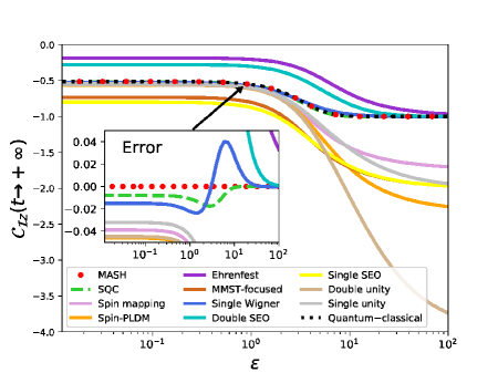
The long-time limits of the adiabatic population difference are shown in Fig. 1 as a function of the energy bias, $\varepsilon$, and are calculated with several different quasiclassical approaches. The other parameters are fixed to $\beta=0.3$, $\Delta=1$, $\alpha=1$, $\Omega=1$, so that the condition for classical nuclei, $\beta\Omega<1$, is satisfied. Shi et al. (2009); Zhu, Liu, and Shi (2013) This parameter choice is also justified by calculations discussed in Ref. Amati, Runeson, and Richardson, 2023, where quasiclassical dynamics in the same parameter regime were found to agree well with numerically exact results with all degrees of freedom treated quantum mechanically. Tanimura (2020); Berkelbach (2020) The validity of our theoretical formula, Eq. 12, for predicting the long-time limit of quasiclassical correlation functions has already been demonstrated by us for this model in another recent work, Amati et al. (2022) where we found that its predictions matched well with dynamical simulations.

The general robustness of quasiclassical approaches for thermalizing correctly in any parameter regime of this model can be ascertained by considering the two parameter limits of $\varepsilon\rightarrow 0$ and $\varepsilon\rightarrow\infty$. Of these extremes, one would expect the $\varepsilon\rightarrow 0$ limit to be the least challenging for quasiclassical approaches, as for our chosen parameter set of the model, the thermal energy is large compared to all other energy scales, such that the quasiclassical description of both electronic and nuclear degrees of freedom should be valid. It is therefore slightly surprising that a significant number of the approaches we tested fail in this regime, including the commonly used Ehrenfest approach. The $\varepsilon\rightarrow\infty$ limit is even more challenging, as this leads to unphysical negative populations associated with the excited state in many quasiclassical approaches [i.e., $\mathcal{C}_{\mathcal{I}z}<-1$], as can be seen in Fig. 1. We do however note that the double SEO and single Wigner approaches, despite still having phase-space regions that correspond to negative populations, do thermalize to the correct physical value in the $\varepsilon\rightarrow\infty$ limit.

The best approaches with regards to their thermalization behaviour for this model are single Wigner, SQC and MASH, which all thermalize reasonably accurately in both the $\varepsilon\rightarrow 0$ and $\varepsilon\rightarrow\infty$ limits. As a result, these approaches are observed to thermalize relatively well for all parameter regimes of the model, as illustrated in Fig. 1. In particular, MASH is seen to exactly reproduce our benchmark result across the whole range.

III.2 An anharmonic model

In order to fully test the effect of inverted potentials on the thermalization behaviour of mean-field approaches, an anharmonic model is needed for which at least one of the diabatic potentials can become unbounded. We choose the reaction-coordinate potentials appearing in Eq. 15 to be

$$U_{\mathrm{RC}}(x_{\mathrm{c}}) =\tfrac{1}{2}\left[\tfrac{1}{2}\Omega^{2}x_{\mathrm{c}}^{2}+\mathrm{e}^{-\Omega(x_{\mathrm{c}}-\bar{x}_{\mathrm{c}})}\right],$$ (19a)

$$\hat{V}_{\mathrm{RC}}(x_{\mathrm{c}}) =\Delta\hat{\sigma}_{x}+\tfrac{\alpha}{2}\left[\tfrac{1}{2}\Omega^{2}x_{\mathrm{c}}^{2}-\mathrm{e}^{-\Omega(x_{\mathrm{c}}-\bar{x}_{\mathrm{c}})}\right]\hat{\sigma}_{z},$$ (19b)

where $0\leq\alpha\leq 1$ determines the strength of the electron-nuclear coupling and we choose the other parameters to be $\Delta=1$, $\Omega=1$, $\bar{x}_{\mathrm{c}}=5$ and $\beta=0.3$. This model is constructed so that the electronic and nuclear subsystems are uncoupled at $\alpha=0$ and the model becomes identical to a previously used electronic predissociation modelRichardson and Thoss (2014); Lawrence and Manolopoulos (2018) at $\alpha=1$. On increasing $\alpha$, we see in Fig. 2 that the red diabatic well at lower energy becomes progressively less bounded. Additionally, the energy gap between the lower and upper adiabatic states increases, which more significantly drives the system into the lower energy adiabat in the long-time limit.

Figure 2: The diabatic potentials associated with the anharmonic model, $\tfrac{1}{4}[1\pm\alpha]\Omega^{2}x_{\mathrm{c}}^{2}+\tfrac{1}{2}[1\mp\alpha]\mathrm{e}^{-\Omega(x_{\mathrm{c}}-\bar{x}_{\mathrm{c}})}$, for several values of the coupling parameter, $\alpha$. The potentials have been vertically shifted such that the lowest energy minimum of the diabats is located at zero. In the case of $\alpha=0$, the two diabatic potentials are identical.

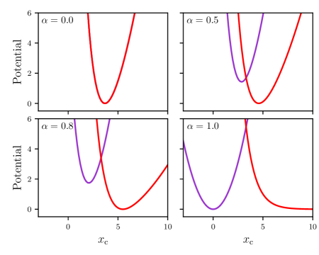
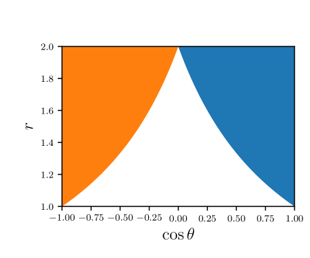
If a trajectory has a large enough negative population in the purple diabat [Fig. 2], so that the contribution from its potential becomes inverted, then the total nuclear force can become unbounded, resulting in the trajectory accelerating off to infinity. This problem can be understood in terms of the mean-field approximation to the state-dependent potential [Eq. 4a], the magnitude of which can become unphysically large through the multiplication of the Cartesian mapping variables with a norm, $r$, greater than one. For this model, this results in the following definition of the effective electron–nuclear coupling associated with these methods: $\alpha_{\rm{eff}}=\alpha r$. Given that that the red diabatic potential shown in Fig. 2 becomes unbounded when $\alpha\geq 1$, we see that this will first occur for the mean-field methods when $\alpha r_{\mathrm{max}}\geq 1$, where $r_{\mathrm{max}}$ is the maximum allowed value of the Cartesian mapping variable norm for that method. We therefore note that the inverted potential problem is particularly problematic for MMST approaches, for which $r_{\rm{max}}=\infty$, so that the nuclear force can become unbounded for any non-zero value of $\alpha$.

Figure 3: The long-time limits of the adiabatic population difference for the anharmonic model introduced in Sec. III.2, as a function of the coupling parameter, $\alpha$. The lines in the figure correspond to our theoretical predictions given by Eq. 12, while the stars are results from dynamical simulations. The simulations were performed by sampling the initial nuclear phase-space variables from Eq. 17 and then propagating the trajectories for $t=400$ with $\eta=2\Omega$ in Eq. 16. Results are only shown in regions where trajectories cannot become unbounded due to inverted potentials.

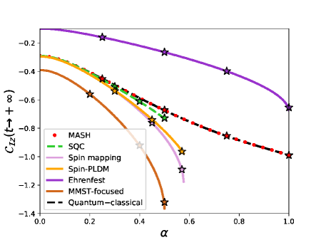
Results for the long-time limits of the adiabatic population difference for this model are shown in Fig. 3 for different quasiclassical methods. The lines in the picture correspond to the theoretical predictions from ergodic theory, while the stars are numerical results from dynamical simulations. Results for each method are only provided for the values of $\alpha$ for which the nuclear force cannot become unbounded because of the problem of inverted potentials. We first note that the long-time limits from the dynamical simulations agree well with our simple formula [Eq. 12], further confirming the validity of applying classical ergodic theory to predict the long-time limit of quasiclassical correlation functions. Importantly, the agreement confirms that the same formula can also be used to accurately predict the long-time limit of MASH correlation functions, even though MASH does not formally have Hamiltonian generated dynamics, as discussed previously in Sec. II.3.

Of all the quasiclassical methods we have tested, MASH is the only one in complete agreement with the quantum–classical benchmark. Its success is largely due to its windowing scheme applied consistently to both the observables and the nuclear force, such that the method does not suffer from the problem of negative populations in either. Although the SQC approach does not deviate too strongly from the exact long-time limit in the parameter regime $0\leq\alpha<0.5$ (in part due to the windowing of its observables), the problem of unbounded inverted potentials contributing to the nuclear force (which unlike for MASH are not windowed) means that SQC becomes unstable in the $0.5\leq\alpha\leq 1$ regime (because $r_{\mathrm{max}}=2$ for SQC, as shown in Appendix B). It would of course be possible to simply discount unbounded trajectories, but this would introduce an ad hoc modification to the method, which may affect some of its formal properties. In addition to MASH, Ehrenfest also does not suffer from the problem of inverted potentials (because $r=1$) and can therefore also be applied in all parameter regimes of the model. However, we see from Fig. 3 that the Ehrenfest long-time populations are highly inaccurate, as was also observed in Fig. 1.

In Sec. IV, we further analyze our long-time limit formula to better understand the deficiencies in the thermalization behaviour of certain methods, as well as the excellent thermalization properties of MASH.

IV Analysis

For the two-state models considered in this paper, the benchmark quantum–classical predictions for the long-time limits of the adiabatic populations are obtained from Eq. 13 using $\hat{A}=\tfrac{1}{2}\hat{\mathcal{I}}_{\mathrm{s}}$ and $\hat{B}=\hat{\sigma}^{\text{ad}}_{z}(x)$. Inserting the expressions for the Hamiltonian [Eqs. 1 and 14] and explicitly performing both the quantum traces and the integrals over the nuclear momenta, we find that

$$\mathcal{C}_{\mathcal{I}z}^{\mathrm{QC}}(t\rightarrow\infty)=-\frac{\Braket{\sinh\left[\beta V_{z}^{\text{ad}}(x)\right]}_{\mathrm{b}}}{\Braket{\cosh\left[\beta V_{z}^{\text{ad}}(x)\right]}_{\mathrm{b}}}.$$ (20)

The phase-space average associated with the state-independent nuclear potential is defined as

$$\langle f(x)\rangle_{\mathrm{b}}=\frac{\int\mathrm{d}x\,\mathrm{e}^{-\beta U(x)}f(x)}{\int\mathrm{d}x\,\mathrm{e}^{-\beta U(x)}},$$ (21)

and we have assumed that $\hat{\rho}_{0}(x,p)$ is normalized, $\int\mathrm{d}x\mathrm{d}p\,\operatorname{tr}_{\rm{s}}[\hat{\rho}_{0}(x,p)]=1$. This expression is most easily derived within the kinematic representation. We show in Appendix A that the same result can be obtained using the Hamiltonian in the adiabatic representation, in the $\hbar\rightarrow 0$ limit.

In the following we calculate the equivalent long-time limit expressions for several quasiclassical methods. In order to perform the electronic phase-space integrals necessary to compare our predictions with Eq. 20, we choose to work with the spin-mapping variables in the adiabatic basis [Eq. 7].

IV.1 Mean-Field Approaches

For mean-field approaches, the long-time limit involves the following operator representations: $A(r,\tilde{\Gamma})=\tfrac{1}{2}\mathcal{I}_{\mathrm{s}}(r)$, $B(r,\tilde{\Gamma})=rS^{\mathrm{ad}}_{z}$ and $\rho_{0}(r,\tilde{\Gamma})=\rho_{0,\mathrm{s}}(r)\rho_{\mathrm{b}}(x,p)$. Inserting these into Eq. 12 and performing some of the phase-space integrals, we find

$$\mathcal{C}^{\text{MF}}_{\mathcal{I}z}(t\rightarrow\infty)=-\int_{0}^{\infty}\mathrm{d}r\,r^{2}\rho_{0,\text{s}}(r)\,\mathcal{I}_{\text{s}}(r)$$

$$\times\Bigg{\langle}\frac{\beta rV^{\text{ad}}_{z}(x)\cosh[\beta rV^{\text{ad}}_{z}(x)]-\sinh[\beta rV^{\text{ad}}_{z}(x)]}{[\beta rV_{z}^{\text{ad}}(x)]^{2}\mathcal{Z}^{\mathrm{MF}}(r)}\Bigg{\rangle}_{\mathrm{b}},$$ (22a)

$$\mathcal{Z}^{\mathrm{MF}}(r)=\Braket{\frac{\sinh{\left[\beta rV_{z}^{\text{ad}}(x)\right]}}{\beta rV^{\text{ad}}_{z}(x)}}_{\mathrm{b}}.$$ (22b)

Comparing Eq. 20 and Eq. 22, we see that the expression for the long-time limit of the mean-field correlation function has the wrong functional form, such that there is no universal expression for $\rho_{0,\text{s}}(r)\mathcal{I}_{\text{s}}(r)$ that guarantees that the corresponding mean-field approach would always thermalize to the quantum–classical benchmark. For a given temperature, a system-specific expression for these functions can however be determined so that Eq. 20 and Eq. 22 agree. This idea has recently been used to design the “ellipsoid mapping”, a new mean-field approach for computing thermal correlation functions that rigorously obeys detailed balance. Amati, Runeson, and Richardson (2023) Such an approach however requires a static calculation to be carried out at thermal equilibrium for each system and temperature of interest, in order to calculate the correct associated expression for $\rho_{0,\text{s}}(r)\mathcal{I}_{\text{s}}(r)$, before any dynamical simulations can be performed.

If we instead decide to only use universal functions for $\rho_{0,\text{s}}(r)\mathcal{I}_{\text{s}}(r)$, then their form can at best be chosen to ensure correct thermalization in certain parameter limits. In the following, we consider the limiting cases of high temperature, low temperature and weak system–bath coupling. For the high-temperature limit ($\beta\rightarrow 0$), we show in Sec. C.1 that mean-field approaches are at best capable of reproducing the benchmark [Eq. 20] up to first order in $\beta$. To achieve this for any two-level system, the condition

$$\frac{1}{3}\int_{0}^{\infty}\mathrm{d}r\,r^{3}\rho_{0,\text{s}}(r)\mathcal{I}_{\text{s}}(r)=1$$ (23)

must be satisfied. Mean-field methods that fulfill Eq. 23 are marked with a tick in the $\beta\rightarrow 0$ column of Table 1. For methods that do not satisfy this condition, the value associated with the left-hand side of Eq. 23 is given, which by comparing Eq. 35a and Eq. 35b is seen to be the multiplicative error in the long-time population difference of the method when $\beta\rightarrow 0$. Incidentally, these errors qualitatively explain the deviations of the long-time limit populations from the quantum–classical benchmark in the $\varepsilon\rightarrow 0$ limit of Fig. 1. While the $\varepsilon\rightarrow 0$ and the $\beta\rightarrow 0$ limits of a spin–boson model do not always coincide, they do so approximately for the parameter regime that we study here.

In the low-temperature limit ($\beta\to\infty$), mean-field approaches can correctly reproduce the long-time limit of correlation functions to at best zeroth order in $\mathrm{e}^{-\beta V_{z}^{\mathrm{ad}}(x)}$. As shown in Sec. C.2, they must then satisfy

$$\int_{0}^{\infty}\mathrm{d}r\,r^{2}\rho_{0,\text{s}}(r)\mathcal{I}_{\text{s}}(r)=1.$$ (24)

Mean-field methods that satisfy Eq. 24 are marked with a tick in the $\beta\rightarrow\infty$ column of Table 1. For methods that do not satisfy this condition, the value associated with the left-hand side of Eq. 24 is given, which is the multiplicative error in the long-time population difference of the method when $\beta\rightarrow\infty$. For strongly asymmetric systems, relaxation in the long-time limit will predominately occur into the lowest potential-energy well, like in the low-temperature limit. This means that our results for $\beta\rightarrow\infty$ can also be used to explain the thermalization behaviour of mean-field methods in the spin–boson model for $\varepsilon\rightarrow\infty$, given in Fig. 1. We note however that the asymptotic approach to the low-temperature limit, which corresponds to the term that is first-order in $\mathrm{e}^{-\beta V_{z}^{\mathrm{ad}}(x)}$, is always wrong for mean-field approaches, as is also observed numerically from our results in Fig. 1.

We show in Sec. C.3 (and also illustrate with crosses for all the mean-field methods in the $\alpha\rightarrow 0$ column of Table 1) that it is not possible to design mean-field methods which consistently thermalize correctly in the weak-coupling limit. Despite this, spin mapping and spin-PLDM appear very accurate in the $\alpha\rightarrow 0$ limit of the anharmonic model [see Fig. 3]. This is because the weak-coupling limit for this particular parameter set of the model also coincides with the $\beta\rightarrow 0$ limit. These methods would not have been as accurate in this limit if we would have instead studied a lower-temperature regime. Let us remark that if the electron–nuclear coupling is identically zero, all methods discussed are able to correctly capture the Rabi oscillations of the isolated electronic subsystem. In this case ergodic theory does not apply, given that the dynamics do not thermalize to equilibrium at long times. Note that this condition is different from the $\alpha\to 0$ limit discussed in Tables 1 and C.3, where the coupling is assumed to be infinitesimal but nonzero.

IV.2 Symmetric quasiclassical windowing (SQC)

For SQC, the potential still retains the same representation as for the mean-field methods [i.e., $\hat{\sigma}^{\mathrm{ad}}_{z}(x)\mapsto rS^{\mathrm{ad}}_{z}$ in Eq. 14], but the observable operators are now represented by the triangular windows, given by Eq. 34 in terms of the spin-mapping variables. Inserting these operator representations into Eq. 12 and performing some of the phase-space integrals gives

$$\mathcal{C}^{\mathrm{SQC}}_{\mathcal{I}z}(t\rightarrow\infty) =\frac{\tilde{\mathcal{C}}^{\mathrm{SQC}}_{\mathcal{I}z}(t\rightarrow\infty)}{\mathcal{N}^{\mathrm{SQC}}(t\rightarrow\infty)},$$ (25a)

$$\tilde{\mathcal{C}}^{\mathrm{SQC}}_{\mathcal{I}z}(t\rightarrow\infty) =-\int_{1}^{2}\mathrm{d}r\,(r-1)$$

$$\times\Braket{\frac{\sinh[\beta V^{\mathrm{ad}}_{z}(x)]\sinh[\beta(r-1)V^{\mathrm{ad}}_{z}(x)]}{\beta rV^{\mathrm{ad}}_{z}(x)\mathcal{Z}^{\mathrm{MF}}(r)}}_{\mathrm{b}},$$ (25b)

$$\mathcal{N}^{\mathrm{SQC}}(t\rightarrow\infty) =\int_{1}^{2}\mathrm{d}r\,(r-1)$$

$$\times\Braket{\frac{\cosh[\beta V^{\mathrm{ad}}_{z}(x)]\sinh[\beta(r-1)V^{\mathrm{ad}}_{z}(x)]}{\beta rV^{\mathrm{ad}}_{z}(x)\mathcal{Z}^{\mathrm{MF}}(r)}}_{\mathrm{b}},$$ (25c)

where $\mathcal{N}^{\mathrm{SQC}}(t)$ is the normalization factor, which is required to ensure that the electronic populations sum to one. Note that we have applied the ergodic theory outlined in Sec. II.4 separately to each term in the ratio of Eq. 25a.

A comparison with Eq. 20 clearly shows that Eq. 25 is not exact, again having the wrong functional form compared to the benchmark quantum–classical long-time limit. However, the advantage of SQC over the other mean-field approaches is that the long-time limit of its correlation function also reproduces the benchmark in the weak-coupling limit,Miller and Cotton (2015) in addition to the high- and low-temperature limits (as indicated in Table 1). More details on the thermalization of SQC in these limits is given in Appendix C. The fact that SQC can simultaneously describe the thermalization correctly in all of these limits explains why it is reasonably accurate for all values of $\varepsilon$ for the spin–boson model in Fig. 1 and accurate in the $\alpha\rightarrow 0$ limit of the anharmonic model in Fig. 2. However for larger values of $\alpha$, there is a clear deviation even before the unbounded inverted potentials appear at $\alpha\geq 0.5$.

IV.3 Mapping approach to surface hopping (MASH)

In MASH, both the potential and observable operators are consistently described through the windowing scheme, $$\hat{\sigma}^{\mathrm{ad}}_{z}(x)\mapsto\operatorname{sgn}(S_{z}^{\mathrm{ad}})$$. Following a strategy similar to the one outlined above for the other methods, we find for the long-time population difference of MASH that

$$\mathcal{C}^{\text{MASH}}_{\mathcal{I}z}(t\rightarrow\infty) =\int_{-1}^{1}\mathrm{d}S_{z}^{\text{ad}}\,\operatorname{sgn}{(S_{z}^{\text{ad}})}\rho^{\mathrm{MASH}}_{\mathrm{eq}}(S_{z}^{\mathrm{ad}}),$$ (26a)

$$\rho^{\mathrm{MASH}}_{\mathrm{eq}}(S_{z}^{\mathrm{ad}}) =\frac{\braket{\mathrm{e}^{-\beta V_{z}^{\mathrm{ad}}(x)\operatorname{sgn}(S^{\mathrm{ad}}_{z})}}_{\mathrm{b}}}{2\Braket{\cosh{[\beta V_{z}^{\text{ad}}(x)]}}_{\mathrm{b}}},$$ (26b)

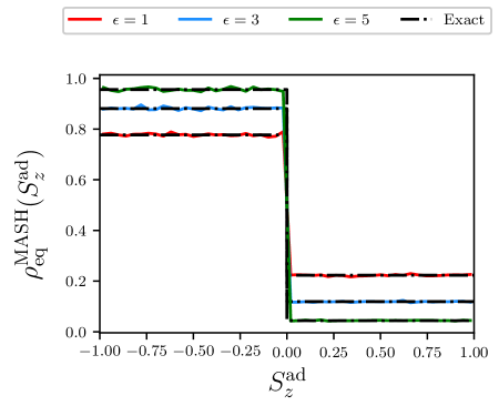
where we have additionally used that the initial distribution for the spin-mapping variables for this correlation function is $$r\rho_{0,\mathrm{s}}=\mathcal{W}_{\mathrm{PP}}(\bm{S}^{\mathrm{ad}})=2|S_{z}^{\mathrm{ad}}| \rho_{\mathrm{eq}}^{\mathrm{MASH}}(S_{z}^{\mathrm{ad}})$$.Mannouch and Richardson (2023) The marginal equilibrium distribution function for MASH, , corresponds to the long-time limit of the conditional probability, given by Eq. 11, with the bath degrees of freedom integrated out.

We first note that our expression for the marginal equilibrium distribution function for MASH agrees with the long-time distribution of $S^{\mathrm{ad}}_{z}$, histogrammed from an ensemble of dynamical MASH trajectories. This is shown in Fig. 4 for the same spin–boson model that was introduced in Sec. III.1, for several values of $\varepsilon$. This marginal distribution constitutes an exact discrete-valued representation of the quantum–classical Boltzmann factors, which demonstrates how MASH effectively quantizes the electronic states, enabling it to thermalize to the benchmark quantum–classical distribution in all cases. The ultimate proof of the long-time accuracy of the MASH dynamics is the fact that Eq. 20 and Eq. 26a are seen to be identical once the integrals over the spin-mapping variables have been performed analytically. To the best of our knowledge, MASH is the only nonequilibrium quasiclassical approach that is guaranteed to thermalize correctly in all nonadiabatic systems in the $\hbar\rightarrow 0$ limit.

Figure 4: The marginal equilibrium distribution function for the mapping variable $S_{z}^{\text{ad}}$, calculated for the spin–boson model defined in Sec. III.1, for several values of the energy bias $\varepsilon$. The colored lines are obtained from histogramming MASH trajectories initialized from Eq. 17 and propagated for $t=500$ with the optimal damping parameter, $\eta=2\Omega$ [Eq. 16]. Additionally, the black dashed lines correspond to the expected results from classical ergodic theory, given by Eq. 26b.

This result may come as a surprise as it is known that MASH does not rigorously obey detailed balance, due to the non-conservation of its weighting factor by the dynamics.Mannouch and Richardson (2023) This raises the question of how MASH can still thermalize correctly. To describe the issue quantitatively, a measure of the microscopic reversibility error (MRE) was defined in Ref. Mannouch and Richardson, 2023. Based on the same ergodicity arguments used here, we show in Appendix D that in the long-time limit the MRE vanishes. This shows that the violation of detailed balance by MASH can only lead to errors at intermediate times, with no adverse effects on its long-time relaxation behaviour.

V Conclusions

In this paper, we presented an analysis of the long-time limits of quasiclassical approaches for simulating nonadiabatic dynamics. We exploited the Hamiltonian structure of the dynamics to make use of results from classical ergodic theory, rigorously accounting for the conservation of the norm of the mapping variables. This allowed us to assess and compare the accuracy of different methods in capturing the correct detailed balance at long times. Our theoretical framework can be applied to any quasiclassical method which is incompressible (i.e., it conserves phase-space volume) non-integrable (i.e., the dynamics cannot be solved analytically) and deterministic.Arnold (1978)

Using our theory, we tested the thermalization behaviour of a wide array of quasiclassical approaches on both the harmonic and anharmonic models. Our analysis revealed that most of the commonly used quasiclassical approaches violate detailed balance and thus do not recover the correct quantum–classical thermal distribution. Errors are particularly large for the anharmonic model, where the problem of inverted potentials meant that trajectories from the majority of quasiclassical approaches were unphysically accelerated off to infinity. Among all of the methods considered, only MASH is guaranteed to predict the exact quantum–classical correlation functions in the long-time limit, to zeroth-order in $\hbar$. This method is therefore capable of solving the long-standing issue of detailed balance (at least in the long-time limit), a problem which has plagued the field of quasiclassical dynamics to date. In addition, because MASH does not suffer from the problem of inverted potentials, it is ideally suited for performing ab-initio nonadiabatic simulations of molecules, where the strongly anharmonic adiabatic potentials would pose a significant challenge to the other quasiclassical approaches.

The main limitation of the original version of MASH, introduced in Ref. Mannouch and Richardson, 2023, is that it was derived only for two-state problems. Recently a multi-state generalization of MASH has been proposed by Runeson and Manolopoulos.Runeson and Manolopoulos (2023) In this version, they modified the observable operators to be more similar to the mean-field approaches, which made it easier for them to generalize the underlying theory to multi-state problems. Like the original MASH approach, it is guaranteed to thermalize correctly in the long-time limit. However, it is not guaranteed to exactly reproduce the short-time dynamics of the quantum–classical Liouville equation, which was the means by which the original MASH approach obtained unique and rigorous prescriptions for the momentum rescalings, treatment of frustrated hops and decoherence corrections. In addition, the measurement of observables is not performed using the same windowing procedure as for the nuclear force, meaning that the two can become inconsistent and the observables may measure negative populations. Whilst the accuracy of the numerical results look promising,Runeson and Manolopoulos (2023) given that the rigorous nature and internal consistency of the original MASH approach was its main advantage over FSSH, we still think that there is more work to be done in order to obtain the ultimate multi-state generalization of MASH.

There may however still be a place for mean-field mapping methods. In contrast to typical molecules in the gas phase, many solid-state systems are characterized by a high degree of electronic coherence. Due to the dense bands of electronic states, the treatment of the nonadiabatic dynamics using mean-field approaches seems the most suitable. From our analysis, we conclude that single-Wigner and SQC would be the best mean-field approaches to use in this case. Given that the electronic structure of solids is fairly harmonic, we also expect that the problem of inverted potentials would not be as severe.

It is interesting to compare the conclusions from our analysis to those obtained in previous work. In Refs. Saller, Kelly, and Richardson, 2019, 2020; Gao et al., 2020, it was observed that the unity methods led to improved accuracy compared to other MMST approaches. Similar improvements were observed in Refs. Runeson and Richardson, 2019, 2020; Mannouch and Richardson, 2020a, b, 2022 for spin-mapping methods, which also treat the identity operator exactly within the mapping. However, most previous studies were performed on harmonic models with reasonably small energy biases. From our analysis in this paper, we observe that for more extreme systems, the quasiclassical approaches that treat the identity operator exactly do not always perform the best, suggesting that other criteria may also be important to consider. For example, a recent analysis performed on the ab-initio exited-state dynamics in ethylene found that the best approaches in this case were those that had the least phase-space volume associated with negative populations.Miyazaki and Ananth (2023)

The long-time accuracy of quasiclassical methods can often be significantly improved by utilizing these techniques within the Nakajima–Zwanzig generalized quantum master equation (GQME) formalism. Kelly et al. (2016); Mulvihill et al. (2019); Montoya-Castillo and Reichman (2016) This approach describes the non-unitary dissipative dynamics of the subsystem in terms of a non-Markovian equation of motion. Memory effects in the GQME are captured by kernels that decay on timescales that are in general much shorter than the typical electronic relaxation times. This means that it is often advantageous to calculate the kernels using quasiclassical methods, instead of obtaining the full dynamics directly. However it has recently been shown that using the GQME is not guaranteed to fix detailed balanceAmati et al. (2022) if the input quasiclassical method is not sufficiently accurate at short times. Given the remarkable long-time accuracy exhibited by MASH, it could be insightful to couple this method to the GQME for determining the importance of non-Markovian dissipative effects in the dynamics, as well as to reduce the cost of quasiclassical simulations through computing short-lived memory kernels.

Recently there has been increased interest in understanding the effect of strong light-matter coupling on the properties of matter. For quantum light, the coupled electron–photon dynamics can be described using quasiclassical approaches, where the photon phase-space variables are initially sampled from a Wigner distribution.Hoffmann et al. (2019a, b); Saller, Kelly, and Geva (2021) While the short-time dynamics is observed to be fairly accurate, the long-time dynamics is known to suffer as a result of unphysical zero-point energy leakage from these quantum modes.Hsieh, Krotz, and Tempelaar (2023) For classical light, the presence of an external driving field breaks the thermalization to the Boltzmann distribution. The dynamics converge at long times to nonequilibrium stationary states which can be described in certain parameter regimes by the Floquet–Gibbs distribution. Engelhardt, Platero, and Cao (2019); Shirai, Mori, and Miyashita (2015) In both cases, our analysis based on classical ergodic theory could be extended in order to analyze how well quasiclassical approaches describe the correct light-modified long-time properties.

Author Declarations

Conflict of Interest

The authors have no conflicts to disclose.

Author Contributions

Graziano Amati: Conceptualization (equal); Formal analysis (equal); Investigation (equal); Methodology (equal); Visualization (equal); Writing – original draft (equal); Writing – review & editing (equal). Jonathan R. Mannouch: Conceptualization (equal); Formal analysis (equal); Investigation (equal); Methodology (equal); Visualization (equal); Writing – original draft (equal); Writing – review & editing (equal). Jeremy O. Richardson: Conceptualization (equal); Formal analysis (supporting); Supervision (lead); Writing – review & editing (equal).

Appendix A Hamiltonian representations

The total Hamiltonian can be expressed in various representations. In the following we demonstrate that our results are independent of these choices.

For simplicity, we perform the analysis in this section on two-state Hamiltonians, although our conclusions are entirely valid for multi-state problems. We start with the Hamiltonian written in the diabatic basis [Eq. 1]. If the classical nuclear limit is first taken before the electronic operators are transformed to the adiabatic basis, we end up in the kinematic representationCotton, Liang, and Miller (2017) [Eq. 14]

$$\hat{H}_{\text{kin}}(x,p)=\frac{p^{2}}{2m}+U(x)+V^{\rm{ad}}_{z}(x)\hat{\sigma}^{\rm{ad}}_{z}(x).$$ (27)

To illustrate that our quantum–classical benchmark [Eq. 13] is identical in both the diabatic and kinematic representations, we compute the quantum–classical partition function using the diabatic representation

$$\begin{split}Z_{\mathrm{QC}}&=\int\mathrm{d}x\mathrm{d}p\,\operatorname{tr}_{\mathrm{s}}[\mathrm{e}^{-\beta\hat{H}(x,p)}]\\ &=\int\mathrm{d}x\mathrm{d}p\,\mathrm{e}^{-\beta p^{2}/2m-\beta U(x)}\operatorname{tr}_{\mathrm{s}}\left[\mathrm{e}^{-\beta\hat{V}(x)}\right]\\ &=\int\mathrm{d}x\mathrm{d}p\,\mathrm{e}^{-\beta p^{2}/2m-\beta U(x)}\left(\mathrm{e}^{-\beta V^{\mathrm{ad}}_{z}(x)}+\mathrm{e}^{\beta V^{\mathrm{ad}}_{z}(x)}\right),\end{split}$$ (28)

where we have used the fact that the trace of the exponential of an operator is the sum of the exponentials of its eigenvalues. This result is clearly identical to that obtained from the kinematic representation, as the only difference is that the potential energy is already diagonal in the latter.

If the order of operations is interchanged so that the transformation to the adiabatic basis is done before the classical nuclear limit is taken, we end up in the adiabatic representation

$$\begin{split}\hat{H}_{\text{ad}}(x,p_{\mathrm{ad}})=\frac{1}{2m}&\left(p_{\mathrm{ad}}+\hbar d(x)\hat{\sigma}^{\rm{ad}}_{y}(x)\right)^{2}\\ &+U(x)+V^{\rm{ad}}_{z}(x)\hat{\sigma}^{\rm{ad}}_{z}(x),\end{split}$$ (29)

where $d(x)=\Braket{\psi_{+}(x)}{\frac{\partial}{\partial x}}{\psi_{-}(x)}$ is the nonadiabatic coupling vector and $p_{\mathrm{ad}}$ is the canonical momentum associated with the adiabatic representation. Factors of $\hbar$, which originate from the nuclear momentum operator, are explicitly retained for the following discussion. Computing the quantum–classical partition function using the adiabatic representation, we find

$$\begin{split}Z_{\mathrm{QC}}^{\mathrm{ad}}&=\int\mathrm{d}x\mathrm{d}p_{\mathrm{ad}}\,\operatorname{tr}_{\mathrm{s}}\left[\mathrm{e}^{-\beta\hat{H}_{\mathrm{ad}}(x,p_{\mathrm{ad}})}\right],\\ &=\int\mathrm{d}x\mathrm{d}p_{\mathrm{ad}}\,\mathrm{e}^{-\beta(p_{\mathrm{ad}}^{2}+\hbar^{2}d(x)^{2})/2m-\beta U(x)}\\ &\quad\times\operatorname{tr}_{\mathrm{s}}\left[\mathrm{e}^{-\beta\left(\hbar d(x)p_{\mathrm{ad}}\hat{\sigma}_{y}^{\mathrm{ad}}(x)/m+\hat{V}_{z}^{\mathrm{ad}}(x)\hat{\sigma}_{z}^{\mathrm{ad}}(x)\right)}\right],\\ &\simeq\int\mathrm{d}x\mathrm{d}p_{\mathrm{ad}}\,\mathrm{e}^{-\beta p_{\mathrm{ad}}^{2}/2m-\beta U(x)}\operatorname{tr}_{\mathrm{s}}\left[\mathrm{e}^{-\beta V_{z}^{\mathrm{ad}}(x)\hat{\sigma}_{z}^{\mathrm{ad}}(x)}\right]\end{split}$$ (30)

where in the final line we take the $\hbar\rightarrow 0$ limit. Is it then seen that Eqs. 28 and 30 are identical in this limit.

Appendix B Operators for SQC in spherical coordinates

In this appendix, we rewrite the two-state SQC representation of the adiabatic population operators in spherical coordinates. Using this result, an analytic expression for the long-time limit of the adiabatic populations can be obtained for this method [Eq. 25]. Unlike most other mapping approaches, the exact form of SQC depends on the representation chosen. We will utilize the adiabatic representation, which has previously been employed in ab initio simulations,Talbot, Head-Gordon, and Cotton (2022) because this is expected to lead to the best possible predictions available from the approach. It is then also easier to compare with MASH, which is always run in the adiabatic representation.

The SQC approach is usually expressed in terms of action–angle variables. These can be transformed to spherical coordinates by combining Eqs. 5 and 7, which leads to

$$rS^{\mathrm{ad}}_{x} =r\sin\theta\cos\phi=2\sqrt{(n_{+}+\gamma)(n_{-}+\gamma)}\cos(q_{+}-q_{-}),$$ (31a)

$$rS^{\mathrm{ad}}_{y} =r\sin\theta\sin\phi=2\sqrt{(n_{+}+\gamma)(n_{-}+\gamma)}\sin(q_{+}-q_{-}),$$ (31b)

$$rS^{\mathrm{ad}}_{z} =r\cos\theta=n_{+}-n_{-},$$ (31c)

where $q_{+}$ and $q_{-}$ are the angle variables for the upper and lower adiabatic states and are initially sampled uniformly in the range $[0,2\pi)$. Additionally, $n_{+}$ and $n_{-}$ are the action variables for the two adiabatic states, sampled from the appropriate triangular window corresponding to the initial electronic population [Eq. 6].Cotton and Miller (2016)

The expression for the windows in spherical coordinates can be determined from the inverse transformation of Eq. 31, which corresponds to

$$n_{+} =\frac{r}{2}(1+\cos\theta)-\gamma,$$ (32a)

$$n_{-} =\frac{r}{2}(1-\cos\theta)-\gamma,$$ (32b)

$$q_{+}-q_{-} =\phi.$$ (32c)

Note that $q_{+}+q_{-}$ is an unimportant cyclic variable conjugate to the conserved radius. The new angle variable $\phi$ is initially sampled uniformally in the range $[0,2\pi)$. Finally, inserting Eq. 32 into Eq. 6, we find that the triangular windows in spherical coordinates are

$$\mathcal{W}_{+}(r,\theta) =h\left(\tfrac{r}{2}(1+\cos\theta)-1\right)h(2-r),$$ (33a)

$$\mathcal{W}_{-}(r,\theta) =h\left(\tfrac{r}{2}(1-\cos\theta)-1\right)h(2-r).$$ (33b)

which are illustrated in Fig. 5. Note that for $r=2$, the SQC windows fill the $\cos\theta$ axis and correspond to the hemispheres of the spin-sphere, which are identical to the windows used in MASH. This connection is unsurprising, as it has already been noted that the weighting factors used in the MASH correlation functions correspond to those for the $r=2$ MMST sphere.Mannouch and Richardson (2023) Finally, in order to find the SQC representations for the $r^{N-1}\rho_{0,\mathrm{s}}(r)$ distribution and the $\hat{\mathcal{I}}_{\mathrm{s}}$ and $\hat{\sigma}_{z}^{\mathrm{ad}}(x)$ operators, linear combinations of Eq. 33 can be taken, leading to

$$r^{N-1}\rho_{0,\mathrm{s}}(r) =h(2-r),$$ (34a)

$$\mathcal{I}_{\mathrm{s}}(r) =h(|rS^{\text{ad}}_{z}|-2+r),$$ (34b)

$$\sigma^{\text{ad}}_{z}(x) =\operatorname{sgn}(S_{z}^{\text{ad}})h(|rS^{\text{ad}}_{z}|-2+r).$$ (34c)

Figure 5: The triangular windows used in SQC expressed in spherical polar coordinates. The blue and orange regions correspond to $W_{+}(r,\theta)$ and $W_{-}(r,\theta)$ respectively, which take the form of spherical caps.

Appendix C Perturbative expansions of the long-time limit

In this appendix, we obtain perturbative expressions for the long-time limit of various quasiclassical correlation functions. These expressions allow us to assess how accurately different methods thermalize in different parameter regimes. Note that it is unnecessary to carry out the following analysis for MASH, because, as proven in Sec. IV.3, the long-time limits of its correlation functions are exact and hence all orders of these perturbative expansions are guaranteed to be correctly reproduced.

C.1 The $\beta\rightarrow 0$ limit

The $\beta\rightarrow 0$ limit allows us to assess how accurately quasiclassical approaches reproduce the long-time limit of correlation functions at high-temperature. Because we are already assuming in this paper that we are in the high-temperature limit with respect to the nuclear degrees of freedom (so that a classical treatment of the bath is valid), we clarify that by the high-temperature limit here we mean relative to the electronic energy scales.

Using the expressions Eqs. 20, 22 and 25, we obtain the following results for the first-order term in the corresponding high-temperature Taylor expansions

$$\mathcal{C}_{\mathcal{I}z}^{\mathrm{QC}}(t\rightarrow\infty) \sim-\beta\langle V_{z}^{\mathrm{ad}}(x)\rangle_{\mathrm{b}},$$ (35a)

$$\mathcal{C}^{\text{MF}}_{\mathcal{I}z}(t\rightarrow\infty) \sim-\frac{\beta}{3}\langle V^{\mathrm{ad}}_{z}(x)\rangle_{\mathrm{b}}\int\mathrm{d}r\,r^{3}\rho_{0,\text{s}}(r)\,\mathcal{I}_{\text{s}}(r),$$ (35b)

$$C^{\text{SQC}}_{\mathcal{I}z}(t\rightarrow\infty) \sim-\beta\langle V_{z}^{\mathrm{ad}}(x)\rangle_{\mathrm{b}}.$$ (35c)

We thus see that SQC is able to correctly thermalize in the high-temperature limit, although we note that this is not the case for all mean-field methods. Comparing Eqs. 35a and 35b leads to the condition expressed in Eq. 23 that must be satisfied for mean-field methods to describe this limit correctly.

While the $\varepsilon\rightarrow 0$ and the $\beta\rightarrow 0$ limits of a spin–boson model do not always coincide, they approximately do for the parameter regime that we study here. This means that these high-temperature limit formulas can be used to understand the thermalization behaviour of quasiclassical approaches in the $\varepsilon\rightarrow 0$ limit of the spin-boson model discussed in Sec. III.1.

C.2 The $\beta\rightarrow\infty$ limit

Here we investigate the low-temperature ($\beta\rightarrow\infty$) limit with respect to the electronic energy scales. We still assume that the temperature is high with respect to the nuclear degrees of freedom, such that it is valid to treat them classically. The zeroth-order terms of these expansions are

$$\mathcal{C}_{\mathcal{I}z}^{\mathrm{QC}}(t\rightarrow\infty) \sim-1,$$ (36a)

$$\mathcal{C}^{\text{MF}}_{\mathcal{I}z}(t\rightarrow\infty) \sim-\int\mathrm{d}r\,r^{2}\rho_{0,\text{s}}(r)\,\mathcal{I}_{\text{s}}(r),$$ (36b)

$$\mathcal{C}_{\mathcal{I}z}^{\mathrm{SQC}}(t\rightarrow\infty) \sim-1.$$ (36c)

We note that SQC also describes the thermalization in the low-temperature regime correctly, while mean-field methods do not unless they satisfy the condition Eq. 24.

In the long-time limit, the system will predominately relax into the lowest potential-energy well in both the $\beta\rightarrow\infty$ and the $\varepsilon\rightarrow\infty$ limits of the spin–boson model. This means that our long-time limit formulas for ${\beta\rightarrow\infty}$ can also be used to understand the thermalization behaviour of quasiclassical approaches in the $\varepsilon\rightarrow\infty$ limit of the spin–boson model discussed in Section III.1. We additionally remark that quasiclassical approaches that reproduce the correct $\beta\rightarrow\infty$ limit are not in general guaranteed to reproduce the right asymptotic approach (apart from MASH), as observed in our numerical results [see in particular Ehrenfest and double SEO in Fig. 1].

C.3 The $\alpha\rightarrow 0$ limit

The weak-coupling limit ($\alpha\rightarrow 0$) leads to a significant simplification of our long-time limit formulas, because in this limit $V^{\mathrm{ad}}_{z}(x)=V_{z}^{(0)}$ becomes independent of the nuclear positions and such terms can be taken outside the phase-space averages, $\braket{\cdots}_{\mathrm{b}}$. This means that identical terms in the numerator and denominator of a fraction that previously belonged in different phase-space integrals now cancel. Performing these simplifications leads to the zeroth-order terms

$$\mathcal{C}_{\mathcal{I}z}^{\mathrm{QC}}(t\rightarrow\infty) \sim-\tanh{(\beta V_{z}^{(0)}}),$$ (37a)

$$\mathcal{C}^{\text{MF}}_{\mathcal{I}z}(t\rightarrow\infty) \sim-\int\mathrm{d}r\,r^{2}\rho_{0,\text{s}}(r)\,\mathcal{I}_{\text{s}}(r)$$

$$\qquad\times\Bigg{[}\coth(\beta rV_{z}^{(0)})-\frac{1}{\beta rV_{z}^{(0)}}\Bigg{]},$$ (37b)

$$C^{\text{SQC}}_{\mathcal{I}z}(t\rightarrow\infty) \sim-\tanh{(\beta V_{z}^{(0)}}).$$ (37c)

We find that SQC is also exact in the weak-coupling limit, as was also shown in Ref. Miller and Cotton, 2015. This time, the mean-field condition depends on $\beta V_{z}^{(0)}$ and so cannot be satisfied in general unless the method is explicitly dependent on this system-dependent variable (similar to Ref. Amati, Runeson, and Richardson, 2023). These results are summarized in the corresponding column of Table 1.

Appendix D Microscopic-reversibility error in MASH

The microscopic-reversibility error (MRE) was introduced as a way of estimating the error in MASH arising from the violation of time-reversal symmetry.Mannouch and Richardson (2023) This arises due to the presence of a weighting factor in the definition of the MASH correlation functions that is not conserved by the dynamics.

For the specific case of the adiabatic population difference studied in this work, the MRE is defined by

$$\left\langle\left[|S^{\mathrm{ad}}_{z}(t)|-|S^{\mathrm{ad}}_{z}|\right]\operatorname{sgn}(S^{\mathrm{ad}}_{z}(t))\right\rangle_{0},$$ (38)

where $\tfrac{1}{2}$ and $\operatorname{sgn}(S_{z}^{\mathrm{ad}})$ are the MASH representations of the $\tfrac{1}{2}\hat{\mathcal{I}}_{\mathrm{s}}$ and $\hat{\sigma}_{z}^{\mathrm{ad}}(x)$ operators respectively, $2|S_{z}^{\mathrm{ad}}|$ is the corresponding MASH weighting factor for this correlation function, and the ensemble average $\braket{\cdots}_{0}$ is defined in Eq. 12b.

Our formula for evaluating the long-time limit of quasiclassical correlation functions [Eq. 12] can be applied here to evaluate the long-time limit of the MRE. Using

$$\int_{-1}^{1}\mathrm{d}S_{z}^{\mathrm{ad}}\,\left\langle\left[S^{\mathrm{ad}}_{z}-\operatorname{sgn}(S^{\mathrm{ad}}_{z})\right]\rho^{\mathrm{MASH}}_{\mathrm{eq}}(S^{\mathrm{ad}}_{z})\right\rangle_{\mathrm{b}}=0$$ (39)

we find that the MRE vanishes in the long-time limit. To obtain this result, we have also used $\langle|S^{\mathrm{ad}}_{z}|\rangle_{0}=1$ and the definitions of the the ensemble average $\braket{\cdots}_{\mathrm{b}}$ and the MASH thermal density given in Eqs. 21 and 26b respectively. This result therefore explains why MASH is able to exactly reproduce the long-time limit of correlation functions despite not rigorously obeying detailed balance.

References

- Matsika and Krause (2011) S. Matsika and P. Krause, “Nonadiabatic events and conical intersections,” Annu. Rev. Phys. Chem. 62, 621–643 (2011).
- Akimov and Prezhdo (2014) A. V. Akimov and O. V. Prezhdo, “Nonadiabatic Dynamics of Charge Transfer and Singlet Fission at the Pentacene/C60 Interface,” J. Am. Chem. Soc. 136, 1599–1608 (2014).
- Magazzù et al. (2018) L. Magazzù, P. Forn-Díaz, R. Belyansky, J.-L. Orgiazzi, M. A. Yurtalan, M. R. Otto, A. Lupascu, C. M. Wilson, and M. Grifoni, “Probing the strongly driven spin-boson model in a superconducting quantum circuit,” Nat. Commun. 9, 1403 (2018).
- Kapral (2015) R. Kapral, “Quantum dynamics in open quantum-classical systems,” J. Phys.-Condens. Mat. 27, 073201 (2015).
- Martens (2016) C. C. Martens, “Surface hopping by consensus,” J. Phys. Chem. Lett. 7, 2610–2615 (2016).
- Runeson et al. (2022a) J. E. Runeson, J. R. Mannouch, G. Amati, M. R. Fiechter, and J. O. Richardson, “Spin-mapping methods for simulating ultrafast nonadiabatic dynamics,” Chimia 76, 582–588 (2022a).
- Tully (1998) J. C. Tully, “Mixed quantum–classical dynamics,” Faraday Discuss. 110, 407–419 (1998).
- Kirrander and Vacher (2020) A. Kirrander and M. Vacher, “Ehrenfest Methods for Electron and Nuclear Dynamics,” in Quantum Chemistry and Dynamics of Excited States (John Wiley & Sons, Ltd, 2020) Chap. 15, pp. 469–497.
- Stock and Thoss (2005) G. Stock and M. Thoss, “Classical description of nonadiabatic quantum dynamics,” Adv. Chem. Phys. 131, 243–376 (2005).
- Tully (2012) J. C. Tully, “Perspective: Nonadiabatic dynamics theory,” J. Chem. Phys. 137, 22A301 (2012).
- Saller, Kelly, and Richardson (2019) M. A. C. Saller, A. Kelly, and J. O. Richardson, “On the identity of the identity operator in nonadiabatic linearized semiclassical dynamics,” J. Chem. Phys. 150, 071101 (2019).
- Runeson and Richardson (2019) J. E. Runeson and J. O. Richardson, “Spin-mapping approach for nonadiabatic molecular dynamics,” J. Chem. Phys. 151, 044119 (2019).
- Mannouch and Richardson (2020a) J. R. Mannouch and J. O. Richardson, “A partially linearized spin-mapping approach for nonadiabatic dynamics. I. Derivation of the theory,” J. Chem. Phys. 153, 194109 (2020a).
- Runeson et al. (2022b) J. E. Runeson, J. E. Lawrence, J. R. Mannouch, and J. O. Richardson, “Explaining the efficiency of photosynthesis: quantum uncertainty or classical vibrations?” J. Phys. Chem. Lett. 13, 3392–3399 (2022b).
- Amati et al. (2022) G. Amati, M. A. Saller, A. Kelly, and J. O. Richardson, “Quasiclassical approaches to the generalized quantum master equation,” J. Chem. Phys. 157, 234103 (2022).
- Parandekar and Tully (2006) P. V. Parandekar and J. C. Tully, “Detailed balance in Ehrenfest mixed quantum-classical dynamics,” J. Chem. Theory Comput. 2, 229–235 (2006).
- Meyer and Miller (1979) H.-D. Meyer and W. H. Miller, “A classical analog for electronic degrees of freedom in nonadiabatic collision processes,” J. Chem. Phys. 70, 3214–3223 (1979).
- Stock and Thoss (1997) G. Stock and M. Thoss, “Semiclassical description of nonadiabatic quantum dynamics,” Phys. Rev. Lett. 78, 578–581 (1997).
- Sun, Wang, and Miller (1998) X. Sun, H. Wang, and W. H. Miller, “Semiclassical theory of electronically nonadiabatic dynamics: Results of a linearized approximation to the initial value representation,” J. Chem. Phys. 109, 7064–7074 (1998).
- Wang et al. (1999) H. Wang, X. Song, D. Chandler, and W. H. Miller, “Semiclassical study of electronically nonadiabatic dynamics in the condensed-phase: Spin-boson problem with Debye spectral density,” J. Chem. Phys. 110, 4828–4840 (1999).
- Kim, Nassimi, and Kapral (2008) H. Kim, A. Nassimi, and R. Kapral, “Quantum-classical Liouville dynamics in the mapping basis,” J. Chem. Phys. 129, 084102 (2008).
- Kelly et al. (2012) A. Kelly, R. van Zon, J. Schofield, and R. Kapral, “Mapping quantum-classical Liouville equation: Projectors and trajectories,” J. Chem. Phys. 136, 084101 (2012).
- Liu et al. (2020) Y. Liu, X. Gao, Y. Lai, E. Mulvihill, and E. Geva, “Electronic dynamics through conical intersections via quasi-classical mapping Hamiltonian methods,” J. Chem. Theory Comput. 16, 4479–4488 (2020).
- Saller, Kelly, and Richardson (2020) M. A. C. Saller, A. Kelly, and J. O. Richardson, “Improved population operators for multi-state nonadiabatic dynamics with the mixed quantum-classical mapping approach,” Faraday Discuss. 221, 150–167 (2020).
- Gao et al. (2020) X. Gao, M. A. C. Saller, Y. Liu, A. Kelly, J. O. Richardson, and E. Geva, “Benchmarking Quasiclassical Mapping Hamiltonian Methods for Simulating Electronically Nonadiabatic Molecular Dynamics,” J. Chem. Theory Comput. 16, 2883–2895 (2020).
- Runeson and Richardson (2020) J. E. Runeson and J. O. Richardson, “Generalized spin mapping for quantum-classical dynamics,” J. Chem. Phys. 152, 084110 (2020).
- Bonella and Coker (2001) S. Bonella and D. F. Coker, “A semiclassical limit for the mapping hamiltonian approach to electronically nonadiabatic dynamics,” J. Chem. Phys. 114, 7778–7789 (2001).
- Amati, Runeson, and Richardson (2023) G. Amati, J. E. Runeson, and J. O. Richardson, “On detailed balance in nonadiabatic dynamics: From spin spheres to equilibrium ellipsoids,” J. Chem. Phys. 158, 064113 (2023).
- Miller and Cotton (2016) W. H. Miller and S. J. Cotton, “Classical molecular dynamics simulation of electronically non-adiabatic processes,” Faraday Discuss. 195, 9–30 (2016).
- Miller and Cotton (2015) W. H. Miller and S. J. Cotton, “Communication: Note on detailed balance in symmetrical quasi-classical models for electronically non-adiabatic dynamics,” J. Chem. Phys 142, 131103 (2015).
- Bellonzi, Jain, and Subotnik (2016) N. Bellonzi, A. Jain, and J. E. Subotnik, “An assessment of mean-field mixed semiclassical approaches: Equilibrium populations and algorithm stability,” J. Chem. Phys. 144, 154110 (2016).
- Tully (1990) J. C. Tully, “Molecular dynamics with electronic transitions,” J. Chem. Phys. 93, 1061–1071 (1990).
- Pechukas (1969) P. Pechukas, “Time-dependent semiclassical scattering theory. II. Atomic collisions,” Phys. Rev. 181, 174 (1969).
- Herman (1984) M. F. Herman, “Nonadiabatic semiclassical scattering. I. Analysis of generalized surface hopping procedures,” J. Chem. Phys. 81, 754–763 (1984).
- Schmidt, Parandekar, and Tully (2008) J. R. Schmidt, P. V. Parandekar, and J. C. Tully, “Mixed quantum-classical equilibrium: Surface hopping,” J. Chem. Phys. 129, 044104 (2008).
- Subotnik, Ouyang, and Landry (2013) J. E. Subotnik, W. Ouyang, and B. R. Landry, “Can we derive Tully’s surface-hopping algorithm from the semiclassical quantum Liouville equation? Almost, but only with decoherence,” J. Chem. Phys. 139, 214107 (2013).
- Kapral (2016) R. Kapral, “Surface hopping from the perspective of quantum–classical liouville dynamics,” Chem. Phys. 481, 77–83 (2016), quantum Dynamics and Femtosecond Spectroscopy dedicated to Prof. Vladimir Y. Chernyak on the occasion of his 60th birthday.
- Mannouch and Richardson (2023) J. R. Mannouch and J. O. Richardson, “A mapping approach to surface hopping,” J. Chem. Phys. 158, 104111 (2023).
- Leaf (1968) B. Leaf, “Weyl transformation and the classical limit of quantum mechanics,” J. Math. Phys. 9, 65–72 (1968).
- Sergi and Kapral (2004) A. Sergi and R. Kapral, “Quantum-classical limit of quantum correlation functions,” J. Chem. Phys. 121, 7565–7576 (2004).
- Saller, Runeson, and Richardson (2021) M. A. C. Saller, J. E. Runeson, and J. O. Richardson, “Path-integral approaches to non-adiabatic dynamics,” in Quantum Chemistry and Dynamics of Excited States: Methods and Applications, edited by L. González and R. Lindh (Wiley, Chichester, 2021) pp. 629–653.
- Müller and Stock (1998) U. Müller and G. Stock, “Consistent treatment of quantum-mechanical and classical degrees of freedom in mixed quantum-classical simulations,” J. Chem. Phys. 108, 7516–7526 (1998).
- Mannouch and Richardson (2020b) J. R. Mannouch and J. O. Richardson, “A partially linearized spin-mapping approach for nonadiabatic dynamics. II. Analysis and comparison with related approaches,” J. Chem. Phys. 153, 194110 (2020b).
- Huo and Coker (2011) P. Huo and D. F. Coker, “Communication: Partial linearized density matrix dynamics for dissipative, non-adiabatic quantum evolution,” J. Chem. Phys. 135, 201101 (2011).
- Hsieh and Kapral (2012) C.-Y. Hsieh and R. Kapral, “Nonadiabatic dynamics in open quantum-classical systems: Forward-backward trajectory solution,” J. Chem. Phys. 137, 22A507 (2012).
- Kim and Rhee (2020) H. W. Kim and Y. M. Rhee, “Two-oscillator mapping modification of the Poisson bracket mapping equation formulation of the quantum–classical Liouville equation,” J. Chem. Phys. 153, 214103 (2020).
- Runeson (2022) J. E. Runeson, Spin-mapping approaches for mixed quantum–classical dynamics, Ph.D. thesis, ETH Zurich (2022).
- Cotton and Miller (2013) S. J. Cotton and W. H. Miller, “Symmetrical windowing for quantum states in quasi-classical trajectory simulations: Application to electronically non-adiabatic processes,” J. Chem. Phys. 139, 234112 (2013).
- Cotton and Miller (2019a) S. J. Cotton and W. H. Miller, “A symmetrical quasi-classical windowing model for the molecular dynamics treatment of non-adiabatic processes involving many electronic states,” J. Chem. Phys. 150, 104101 (2019a).
- Cotton and Miller (2016) S. J. Cotton and W. H. Miller, “A new symmetrical quasi-classical model for electronically non-adiabatic processes: Application to the case of weak non- adiabatic coupling,” J. Chem. Phys 145, 144108 (2016).
- Cotton and Miller (2019b) S. J. Cotton and W. H. Miller, “Trajectory-adjusted electronic zero point energy in classical meyer-miller vibronic dynamics: Symmetrical quasiclassical application to photodissociation,” J. Chem. Phys. 150, 194110 (2019b).
- Cotton, Liang, and Miller (2017) S. J. Cotton, R. Liang, and W. H. Miller, “On the adiabatic representation of Meyer-Miller electronic-nuclear dynamics,” J. Chem. Phys. 147, 064112 (2017).
- Domcke, Yarkony, and Köppel (2004) W. Domcke, D. R. Yarkony, and H. Köppel, eds., Conical Intersections: Electronic Structure, Dynamics and Spectroscopy (World Scientific, Singapore, 2004).
- Berkovitz, Frigg, and Kronz (2006) J. Berkovitz, R. Frigg, and F. Kronz, “The ergodic hierarchy, randomness and Hamiltonian chaos,” Stud. Hist. Philos. Sci. B - Stud. Hist. Philos. Mod. Phys. 37, 661–691 (2006).
- Hawkins (2021) J. Hawkins, Ergodic Dynamics: From Basic Theory to Applications, Graduate Texts in Mathematics (Springer Nature Switzerland, Cham, 2021).
- Evans, Searles, and Williams (2009) D. J. Evans, D. J. Searles, and S. R. Williams, “Dissipation and the relaxation to equilibrium,” J. Stat. Mech. Theory Exp. 2009, P07029 (2009).
- Mauri, Car, and Tosatti (1993) F. Mauri, R. Car, and E. Tosatti, “Canonical Statistical Averages of Coupled Quantum-Classical Systems,” Europhys. Lett. 24, 431 (1993).
- Nielsen, Kapral, and Ciccotti (2001) S. Nielsen, R. Kapral, and G. Ciccotti, “Statistical mechanics of quantum-classical systems,” J. Chem. Phys. 115, 5805–5815 (2001).
- Tuckerman (2010) M. E. Tuckerman, Statistical Mechanics: Theory and Molecular Simulation (Oxford University Press, 2010).
- Leggett et al. (1987) A. J. Leggett, S. Chakravarty, A. T. Dorsey, M. P. A. Fisher, A. Garg, and W. Zwerger, “Dynamics of the dissipative two-state system,” Rev. Mod. Phys. 59, 1 (1987).
- Thoss, Wang, and Miller (2001) M. Thoss, H. Wang, and W. H. Miller, “Self-consistent hybrid approach for complex systems: Application to the spin-boson model with Debye spectral density,” J. Chem. Phys. 115, 2991 (2001).
- Shi et al. (2009) Q. Shi, L. Chen, G. Nan, R. Xu, and Y. Yan, “Electron transfer dynamics: Zusman equation versus exact theory,” J. Chem. Phys. 130 (2009).
- Zhu, Liu, and Shi (2013) L. Zhu, H. Liu, and Q. Shi, “A new method to account for the difference between classical and quantum baths in quantum dissipative dynamics,” New J. Phys. 15, 095020 (2013).
- Tanimura (2020) Y. Tanimura, “Numerically “exact” approach to open quantum dynamics: The hierarchical equations of motion (HEOM),” J. Chem. Phys. 153, 020901 (2020).
- Berkelbach (2020) T. C. Berkelbach, “A python package for reduced density matrix techniques,” https://github.com/berkelbach-group/pyrho (2020).
- Richardson and Thoss (2014) J. O. Richardson and M. Thoss, “Non-oscillatory flux correlation functions for efficient nonadiabatic rate theory,” J. Chem. Phys. 141, 074106 (2014).
- Lawrence and Manolopoulos (2018) J. E. Lawrence and D. E. Manolopoulos, “Analytic continuation of Wolynes theory into the Marcus inverted regime,” J. Chem. Phys. 148, 102313 (2018).
- Arnold (1978) V. I. Arnold, Mathematical methods of classical mechanics (Springer-Verlag, New York, 1978).
- Runeson and Manolopoulos (2023) J. E. Runeson and D. E. Manolopoulos, “A multi-state mapping approach to surface hopping,” (2023), arXiv:2305.08835 .
- Mannouch and Richardson (2022) J. R. Mannouch and J. O. Richardson, “A partially linearized spin-mapping approach for simulating nonlinear optical spectra,” J. Chem. Phys. 156, 024108 (2022).
- Miyazaki and Ananth (2023) K. Miyazaki and N. Ananth, “Nonadiabatic simulations of photoisomerization and dissociation in ethylene using ab initio classical trajectories,” (2023), arXiv:2306.10195 .
- Kelly et al. (2016) A. Kelly, A. Montoya-Castillo, L. Wang, and T. E. Markland, “Generalized quantum master equations in and out of equilibrium: When can one win?” J. Chem. Phys. 144, 184105 (2016).
- Mulvihill et al. (2019) E. Mulvihill, X. Gao, Y. Liu, A. Schubert, B. D. Dunietz, and E. Geva, “Combining the mapping Hamiltonian linearized semiclassical approach with the generalized quantum master equation to simulate electronically nonadiabatic molecular dynamics,” J. Chem. Phys. 151, 074103 (2019).
- Montoya-Castillo and Reichman (2016) A. Montoya-Castillo and D. R. Reichman, “Approximate but accurate quantum dynamics from the Mori formalism: I. Nonequilibrium dynamics,” J. Chem. Phys. 144, 184104 (2016).
- Hoffmann et al. (2019a) N. M. Hoffmann, C. Schäfer, A. Rubio, A. Kelly, and H. Appel, “Capturing vacuum fluctuations and photon correlations in cavity quantum electrodynamics with multitrajectory Ehrenfest dynamics,” Phys. Rev. A 99, 063819 (2019a).
- Hoffmann et al. (2019b) N. M. Hoffmann, C. Schäfer, N. Säkkinen, A. Rubio, H. Appel, and A. Kelly, “Benchmarking semiclassical and perturbative methods for real-time simulations of cavity-bound emission and interference,” J. Chem. Phys. 151, 244113 (2019b).
- Saller, Kelly, and Geva (2021) M. A. C. Saller, A. Kelly, and E. Geva, “Benchmarking Quasiclassical Mapping Hamiltonian Methods for Simulating Cavity-Modified Molecular Dynamics,” J. Phys. Chem. Lett. 12, 3163–3170 (2021).
- Hsieh, Krotz, and Tempelaar (2023) M.-H. Hsieh, A. Krotz, and R. Tempelaar, “A mean-field treatment of vacuum fluctuations in strong light–matter coupling,” J. Phys. Chem. Lett. 14, 1253–1258 (2023).
- Engelhardt, Platero, and Cao (2019) G. Engelhardt, G. Platero, and J. Cao, “Discontinuities in Driven Spin-Boson Systems due to Coherent Destruction of Tunneling: Breakdown of the Floquet-Gibbs Distribution,” Phys. Rev. Lett. 123, 120602 (2019).
- Shirai, Mori, and Miyashita (2015) T. Shirai, T. Mori, and S. Miyashita, “Condition for emergence of the Floquet-Gibbs state in periodically driven open systems,” Phys. Rev. E 91, 030101 (2015).
- Talbot, Head-Gordon, and Cotton (2022) J. J. Talbot, M. Head-Gordon, and S. J. Cotton, “The symmetric quasi-classical model using on-the-fly time-dependent density functional theory within the tamm–dancoff approximation,” Mol. Phys. 121, e2153761 (2022).
- Note (1) Our derivation is similar to that used in Ref. \rev@citealpnumMiller2015SQC, but we believe it to be more rigorous as we explicitly take account of the conserved norm of the mapping variables.