Leveraging World Model Disentanglement in Value-Based Multi-Agent Reinforcement Learning

Abstract

In this paper, we propose a novel model-based multi-agent reinforcement learning approach named Value Decomposition Framework with Disentangled World Model to address the challenge of achieving a common goal of multiple agents interacting in the same environment with reduced sample complexity. Due to scalability and non-stationarity problems posed by multi-agent systems, model-free methods rely on a considerable number of samples for training. In contrast, we use a modularized world model, composed of action-conditioned, action-free, and static branches, to unravel the environment dynamics and produce imagined outcomes based on past experience, without sampling directly from the real environment. We employ variational auto-encoders and variational graph auto-encoders to learn the latent representations for the world model, which is merged with a value-based framework to predict the joint action-value function and optimize the overall training objective. We present experimental results in Easy, Hard, and Super-Hard StarCraft II micro-management challenges to demonstrate that our method achieves high sample efficiency and exhibits superior performance in defeating the enemy armies compared to other baselines.

1 Introduction

As teams of agents expand in size, so does their potential for tackling increasingly intricate tasks. However, the growth in potential is accompanied by a significant rise in the complexity of coordinating the actions and interactions of these agents, considering various constraints and dynamic environments. In light of these challenges, this work proposes to extend the current state-of-the-art approaches, based on latent imagination with world models (Hafner et al. 2022), to multi-agent reinforcement learning (MARL) with the key concept of disentanglement, which facilitates effective scaling to unprecedented multi-agent team sizes and problem complexities.

Recently, model-based reinforcement learning (MBRL) has demonstrated sample efficiency and scalability in handling large single-agent tasks (Xu et al. 2018; Hafner et al. 2020, 2022; Yang and Wang 2020; Luo et al. 2022). We explore its application to MARL with an emphasis on latent space generative models, as each agent may only have access to local observations, suffering from the partial observability issue. The majority of applied MARL research has been centered around model-free methods (Tampuu et al. 2017; Lowe et al. 2017; Iqbal and Sha 2018; Zhou et al. 2020; Jeon et al. 2022), while model-based algorithmic studies are still slowly progressing from simple stochastic games to more complex scenarios (Brafman and Tennenholtz 1999, 2003; Zhang, Yang, and Başar 2021). Training model-based policies can be challenging across various domains (Shen et al. 2020). In multi-agent systems, changes occurring around an agent are frequently uncontrollable due to simultaneous interactions with other agents. This leads to a complex learning problem for holistic models, while a recent study on modular representation attempted to decouple the environment dynamics into passive and active components (Pan et al. 2022). Inspired by their work, we maintain three branches within our world model: action-conditioned, action-free, and static. Each branch tackles a unique learning task, including grasping common interaction-free (static) state features, identifying passive (action-free) forces surrounding an agent, and understanding the full complexity of the active (action-conditioned) control system. The predictions of the branches are synergistic and produce informative latent space roll-outs, which are learned by variational and graph convolutional auto-encoders. Combined with individual action values from the joint agent network, the simulated roll-outs are passed into a mixing network, which adopts value decomposition techniques for estimating joint value functions. To the extent of our knowledge, our study marks the first endeavor to leverage the disentanglement of latent representations in MARL.

We evaluate our method on the StarCraft II MARL benchmarks (Samvelyan et al. 2019). We have constantly observed its performance matching or surpassing the state-of-the-art with lower sample complexity. The most significant improvement is evident in a group of environments classified as Super-Hard. They are characterized by a high diversity of unit types involved in complicated interactions and scalability problems that previous approaches struggled with. Our method consistently develops winning strategies for such challenges, while competing algorithms nearly fail to learn with regular sample sizes. This reinforces the importance of our disentanglement approach for large-scale MARL tasks.

2 Related Work

Model-Based Reinforcement Learning.

A fundamental concept in MBRL is the environment model (Luo et al. 2022). It is an abstraction of the environment dynamics, formulated as a Markov decision process (MDP). The agent has the ability to imagine, which means it can generate simulated samples in the environment model. This reduces the interactions with the real environment and improves sample efficiency (Xu et al. 2018; Janner et al. 2019). As a class of the environment model, world models can be applied to learning representations and behaviors (Watter et al. 2015; Pan et al. 2022). Built on the framework of PlaNet (Hafner et al. 2019), Dreamer (Hafner et al. 2023) uses a world model to train the agent with latent imaginations, efficiently predicting long-term behaviors. Meanwhile, the development of multi-agent MBRL has mainly focused on theoretical analyses (Bai and Jin 2020; Zhang et al. 2020; Yang and Wang 2020). Existing algorithms in this field rely heavily on specific prior knowledge such as information on states and adversaries (Brafman and Tennenholtz 2003; Park, Cho, and Kim 2019; Zhang et al. 2021), which can be inaccessible in many scenarios. By contrast, our method constructs models to estimate the prior and posterior distributions of the states, without the need to access enemies’ information.

Value-Based MARL Methods.

A large class of algorithms applied in MARL are value-based methods. They typically compute value function estimates and differ in the extent of centralization. In a fully decentralized scenario (Tan 1997; Tampuu et al. 2017), each agent improves its own policy assuming a stationary environment. Because it fails to account for the behaviors of other agents, this assumption cannot hold (Yang and Wang 2020). There is no theoretical guarantee that an independent learning algorithm will converge in MARL (Zhang, Yang, and Başar 2021). Alternatively, centralized controllers have been applied to gathering the joint observations and actions of the agents (Boutilier 1996; Guestrin, Lagoudakis, and Parr 2002; Kok and Vlassis 2006). They minimize the non-stationarity problem at the cost of scalability, meaning that the joint action space expands exponentially with respect to the number of agents.

Recent studies attempted to design MARL algorithms that lie between the two extremes of decentralization (Yang, Borovikov, and Zha 2019; Son et al. 2019; Rashid et al. 2020; Wang et al. 2020b, c), according to Centralized Training with Decentralized Execution (CTDE) (Kraemer and Banerjee 2016). CTDE stipulates that agents are allowed to exchange information with other agents only during training and they must act in a decentralized manner during execution. Following this paradigm, VDN (Sunehag et al. 2017) uses a joint value function $Q_{tot}$ for agents to learn, and QMIX (Rashid et al. 2018) constructs a mixing network for estimating $Q_{tot}$ with a monotonicity constraint. In our approach, a value factorization framework is employed to mix the agents’ individual action values. It receives the outputs from the disentangled representation learning process, which infers future states using informative simulated roll-outs. It can therefore predict real-world dynamics and approximate the global value function with high accuracy.

3 Background

Dec-POMDP

When agents engage in a task, it is possible that each of them has a limited field of view. The decentralized partially observable Markov decision process (Dec-POMDP) is appropriate for modeling collaborative agents in a partially observable environment (Oliehoek and Amato 2016).

Definition 3.1

A Dec-POMDP is defined by a tuple $M:=\langle\mathcal{S},\mathcal{A},\mathcal{N},T,\mathcal{Z},O,R,\gamma\rangle$ where $\mathcal{S}$ is the state space of all agents, $\mathcal{A}$ is the joint action space of all agents, $\mathcal{N}=\{1,...,N\}$ represents the set of $N$ agents, $T$ is the state transition function, $\mathcal{Z}$ represents the observation space, $O$ is the observation function, $R$ is the reward function, and $\mathit{\gamma}\in[0,1]$ represents the discount factor w.r.t. time.

At time step $t$, each agent $i\in\mathcal{N}$ chooses an action $a^{i}$ from its own action space $\mathcal{A}^{i}$ to form the joint action $\mathbf{a}\in\mathcal{A}$, where $\mathbf{a}:=(a^{1},...,a^{N})$ and $\mathcal{A}:=\times_{i\in\mathcal{N}}\mathcal{A}^{i}$. Then the environment moves from $s$ to $s^{\prime}$ based on $T(s^{\prime}|s,\mathbf{a}):\mathcal{S}\times\mathcal{A}\times\mathcal{S}\to[0,1].$ Every agent $i$ draws an observation $z\in\mathcal{Z}$ according to $O(s,i):\mathcal{S}\times\mathcal{N}\to\mathcal{Z}$ because of partial observability. $i$ has its own action-observation history, denoted by $\tau^{i}\in\mathcal{T}:=(\mathcal{Z}\times\mathcal{A})^{*}$, and selects $a^{i}$ by its policy $\pi^{i}(a^{i}|\tau^{i}):\mathcal{T}\times\mathcal{A}\to[0,1].$ The learning goal is to maximize the expected return by optimizing the joint policy ${\pi}=(\pi^{1},...,\pi^{N})$. The joint action-value function of ${\pi}$ is $Q^{\pi}(s_{t},\mathbf{a}_{t})=\mathbb{E}_{s_{t+1:\infty},\mathbf{a}_{t+1:\infty}}[G_{t}|s_{t},\mathbf{a}_{t}]$, where $G_{t}=\sum^{\infty}_{k=0}\gamma^{k}r_{t+k}$ is the discounted return; $r_{t+k}$ is the reward computed by $R$ for all agents at time step $t+k$.

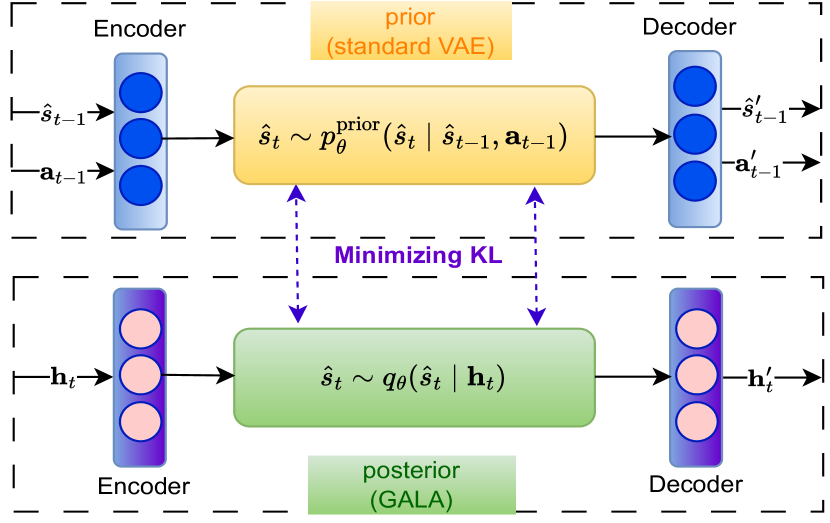
((a))

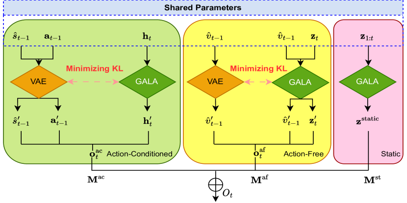
((b))

Figure 1: The learning processes and the structure of the modularized world model. (a) Using VAE and GALA to learn the prior and the posterior in the KL term. The KL distance between the distributions connected by the purple dotted line is minimized. $\mathbf{h}_{t}$ can be viewed as a function of $\hat{s}_{t-1},\mathbf{a}_{t-1},$ and $\mathbf{z}_{t}$. (b) The three modules of the world model with shared parameters.

Value Decomposition and Individual-Global-Max

Based on the CTDE paradigm, value decomposition is an effective technique deployed in MARL algorithms since it encourages collaboration between agents. To apply this technique, we need to define the Individual-Global-Max:

Definition 3.2

Let $\mathcal{A}$ be the joint action space and $\mathcal{T}$ be the joint action-observation history space. Denote the agents’ joint action-observation histories as $\boldsymbol{\tau}\in\mathcal{T}$ and their joint actions as $\mathbf{a}\in\mathcal{A}$. Given the joint action-value function $Q_{tot}:\mathcal{T}\times\mathcal{A}\to\mathbb{R},$ if there exist individual $\{Q_{i}:\mathcal{T}^{i}\times\mathcal{A}^{i}\to\mathbb{R}\}_{i\in\{1,...,N\}}$ such that the following holds:

$$\operatorname*{arg\,max}_{\mathbf{a}\in\mathcal{A}}Q_{tot}(\boldsymbol{\tau},\mathbf{a})=\begin{bmatrix}\operatorname*{arg\,max}_{a^{1}}Q_{1}(\tau^{1},a^{1})\\ \vdots\\ \operatorname*{arg\,max}_{a^{N}}Q_{N}(\tau^{N},a^{N})\end{bmatrix}$$ (1)

then $\{Q_{i}\}_{i\in\{1,...,N\}}$ satisfy the Individual-Global-Max (IGM) condition for $Q_{tot}$ with $\boldsymbol{\tau}$, which means $Q_{tot}(\boldsymbol{\tau},\mathbf{a})$ can be decomposed by $\{Q_{i}\}_{i\in\{1,...,N\}}$.

IGM guarantees that a MARL task can be solved in a decentralized manner as long as local and global action-value functions are consistent (Son et al. 2019).

4 Method

When multiple agents are interacting with each other simultaneously, the environment dynamics can be more sophisticated than in single-agent scenarios. To learn latent dynamics models effectively, we can leverage disentangled representation learning (Goyal et al. 2021; Pan et al. 2022). We hereby introduce a novel model-based multi-agent reinforcement learning algorithm named Value De-composition Framework with Disentangled World Model (VDFD). Specifically, the world model is decomposed into three modules: an action-conditioned (controllable) branch that responds to and depends on the actions of the agents, an action-free (non-controllable) branch that is independent of the agents’ behaviors, and a static branch that consists of environmental features and remains unchanged.

In this section, we analyze how the variational lower bound for the latent state inference in the world model can be deduced and optimized when the environment is modeled as Dec-POMDP. We then discuss the details of world model disentanglement. Next, we elaborate on the entire workflow of VDFD which consists of two parts, world model imagination and reinforcement learning with value function factorization. Lastly, we derive the overall learning objective by summing up the loss functions of different components.

Disentangling the World Model for Representation Learning

Since the global state $s$ is inaccessible to agents outside the centralized training phase, we need to infer the latent state $\hat{s}$ from local actions $\mathbf{a}$ and observations $\mathbf{z}$. We implement a variational auto-encoder (VAE) and a variational graph auto-encoder (VGAE) to approximate the prior and posterior distributions of $\hat{s}$, which is a crucial step in maximizing the evidence lower bound for Dec-POMDP. To learn compact and accurate representations of a multi-agent environment, we disentangle dynamic and static components, denoted as $d$ and $\mathbf{z}^{\text{static}}$, from the world model and train them jointly. The mixed dynamics $d$ of the model can be decoupled into an action-conditioned branch, which corresponds to the state transition $\hat{s}_{t}\sim q(\cdot|\hat{s}_{t-1},\mathbf{a}_{t-1},\mathbf{z}_{t})$, and an action-free branch, which is beyond the control of the agents and can therefore be separated from their joint actions. The non-controllable transition can be modeled as $\hat{v}_{t}\sim q(\cdot|\hat{v}_{t-1},\mathbf{z}_{t})$. The roll-outs from decoupled branches are jointly conveyed to the value factorization framework for centralized training.

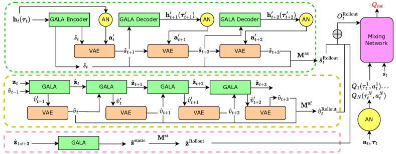
Figure 2: The overall architecture of the VDFD model. The modules enclosed by green, yellow, and pink dashed lines represent the action-conditioned, action-free, and static branches, respectively. The bright yellow circle denotes the agent network, which implements the joint policy for all agents. The joint actions can therefore be extracted from it.

Deriving the Variational Lower Bound.

To perform latent space inference in Dec-POMDP, we need to deduce the evidence lower bound (ELBO) corresponding to this setting. Inspired by the probabilistic approach in (Huang et al. 2020), we create two approximate functions $q_{\pi}(\cdot)$ and $q_{\theta}(\cdot)$, where $\theta$ represents the learnable parameter, $q_{\pi}(\cdot)$ is used for approximating the optimal joint policy, and $q_{\theta}(\cdot)$ is the inference function for latent states. When we keep $q_{\theta}(\cdot)$ fixed, $q_{\pi}(\cdot)$ can be trained using soft Q-learning or vanilla Q-learning. When we fix $q_{\pi}(\cdot)$ as the optimal policy, $q_{\theta}(\cdot)$ can be learned for the latent space. Given time steps $t\in[0,T]$, joint actions $\mathbf{a}\in\mathcal{A}$ and joint observations $\mathbf{z}\in\mathcal{Z}$, we can define the approximate posterior as $q_{\theta}(\hat{s}_{t}|\hat{s}_{t-1},\mathbf{a}_{t-1},\mathbf{z}_{t})$. This function is used to infer the latent states. $\hat{s}_{t}$ is an abstract representation of the agents’ local observations, which indicates that $\mathbf{z}_{t}\sim p(\mathbf{z}_{t}|\hat{s}_{t})$. We can then derive the ELBO of Dec-POMDP, $\mathcal{L}_{\text{ELBO}}(\mathbf{a}_{0:T},\mathbf{z}_{1:T})$, as below. The full deduction procedures can be found in Appendix B.

$$\log p(\mathbf{a}_{0:T},\mathbf{z}_{1:T})$$

$$=\log\mathbb{E}_{q_{\theta}(\hat{s}_{1:T}|\mathbf{a}_{0:T},\mathbf{z}_{1:T})}\left[\frac{p(\hat{s}_{1:T},\mathbf{a}_{0:T},\mathbf{z}_{1:T})}{q_{\theta}(\hat{s}_{1:T}|\mathbf{a}_{0:T},\mathbf{z}_{1:T})}\right]$$

$$\geq\mathbb{E}_{q_{\theta}(\hat{s}_{1:T}|\mathbf{a}_{0:T},\mathbf{z}_{1:T})}\log\left[\frac{p(\hat{s}_{1:T},\mathbf{a}_{0:T},\mathbf{z}_{1:T})}{q_{\theta}(\hat{s}_{1:T}|\mathbf{a}_{0:T},\mathbf{z}_{1:T})}\right]$$

$$\approx\sum_{t=1}^{T}\{\log\left[p(\mathbf{a}_{t}|\mathbf{z}_{t})\right]+\log\left[p(\mathbf{z}_{t}|\hat{s}_{t})\right]$$

$$\phantom{=}\,-\mathcal{D}_{\text{KL}}\left[q_{\theta}(\hat{s}_{t}|\hat{s}_{t-1},\mathbf{a}_{t-1},\mathbf{z}_{t})\parallel p(\hat{s}_{t}|\hat{s}_{t-1},\mathbf{a}_{t-1})\right]\}$$ (2)

Optimizing the ELBO.

We investigate each term in the sum of Eq.2 to maximize the ELBO. First, $\log\left[p(\mathbf{a}_{t}|\mathbf{z}_{t})\right]$ stands for the joint policy that is independent of the state inference. The second term, $\log\left[p(\mathbf{z}_{t}|\hat{s}_{t})\right]$, indicates that the latent states contain the information from which the local observations can be derived. The last term denotes the negative Kullback-Leibler (KL) divergence, which implies that the KL distance between the approximates of posterior and prior should be minimized in the optimization process. As the actual prior $p(\hat{s}_{t}|\hat{s}_{t-1},\mathbf{a}_{t-1})$ is unknown, we introduce a generative function $p^{\text{prior}}_{\theta}(\hat{s}_{t}|\hat{s}_{t-1},\mathbf{a}_{t-1})$ to estimate the prior.

Using Generative Models.

We apply generative models to learning $p^{\text{prior}}_{\theta}(\hat{s}_{t}|\hat{s}_{t-1},\mathbf{a}_{t-1})$ and $q_{\theta}(\hat{s}_{t}|\hat{s}_{t-1},\mathbf{a}_{t-1},\mathbf{z}_{t})$ in the KL term. We construct a VAE for the prior $p^{\text{prior}}_{\theta}(\cdot)$. It takes in the past state, $\hat{s}_{t-1}$, and past actions of all agents, $\mathbf{a}_{t-1}$, to compute the prior distribution of the current state. The prior latent state is denoted $\hat{s}_{t}\sim p^{\text{prior}}_{\theta}(\hat{s}_{t}\mid\hat{s}_{t-1},\mathbf{a}_{t-1}).$

We employ a variant of the VGAE named GALA (Park et al. 2019) for the posterior $q_{\theta}(\cdot)$ to improve the computational efficiency of state inference. GALA is a completely symmetric auto-encoder that combines traditional VAE structure with a Graph Convolutional Network (GCN) encoder (Kipf and Welling 2016). Additionally, it has a special decoder that performs Laplacian sharpening, which is a counterpart to the encoder that conducts Laplacian smoothing. Unlike previous VGAEs that only use an affinity matrix of the GCN in the decoding phase, GALA is able to directly reconstruct the feature matrix of the nodes. Consequently, it captures the information on the relationship between nodes. Because GALA leverages GCN, it ensures that the number of parameters to be trained remains constant so long as the feature dimension of the nodes remains stable, irrespective of the growth in the number of agents. We use recurrent neural networks (RNNs) to implement the agent network in Dec-POMDP. We denote the hidden outputs of the RNN for agent $i$ and for the whole network as $h^{i}_{t}$ and $\mathbf{h}_{t}$, respectively. We interpret $h^{i}_{t}$ as the integration of all past knowledge specific to agent $i$, and assume that $\mathbf{h}_{t}$ collectively encapsulates all the past information of the environment. By this assumption, we can reformulate the approximate posterior $q_{\theta}(\cdot|\hat{s}_{t-1},\mathbf{a}_{t-1},\mathbf{z}_{t})$ as $q_{\theta}(\cdot|\mathbf{h}_{t})$. Initially, the posterior latent state is $\hat{s}_{t}\sim q_{\theta}(\hat{s}_{t}|\hat{s}_{t-1},\mathbf{a}_{t-1},\mathbf{z}_{t}).$ With the reparameterization, it can be transformed into $\hat{s}_{t}\sim q_{\theta}(\hat{s}_{t}|\mathbf{h}_{t}).$ Figure 1(a) illustrates the learning behaviors of the generative models.

Modules of the World Model.

We expatiate on our own version of world model disentanglement. At time step $t$, we define the environment dynamics as $d_{1:t}$. By dividing $d_{1:t}$ into a branch of action-conditioned latent states $\hat{s}_{1:t}$ and a branch of action-free latent states $\hat{v}_{1:t}$, we aim at analyzing interactions and understanding relationships between them. We apply the aforementioned generative models to them, as shown in Figures 1(a) and 1(b). Within the action-conditioned branch, we have the prior representations modeled as $\hat{s}_{t}\sim p^{\text{prior}}_{\theta}(\hat{s}_{t}|\hat{s}_{t-1},\mathbf{a}_{t-1})$ and the posteriors as $\hat{s}_{t}\sim q_{\theta}(\hat{s}_{t}|\mathbf{h}_{t}).$ We seek to minimize the KL divergence between them. Inside the action-free branch, we model the priors as $\hat{v}_{t}\sim p^{\text{prior}}_{\theta}(\hat{v}_{t}|\hat{v}_{t-1})$ and the posteriors as $\hat{v}_{t}\sim q_{\theta}(\hat{v}_{t}|\hat{v}_{t-1},\mathbf{z}_{t})$, minimizing the KL distance as well. Lastly, the static branch incorporates the observations denoted as $\mathbf{z}_{1:t}$. Because it has no priors or posteriors, we only use GALA for representation learning. Denote the outputs of action-conditioned, action-free, and static branches as $\mathbf{o}_{t}^{\text{ac}}$, $\mathbf{o}_{t}^{\text{af}}$, and $\mathbf{z}^{\text{static}}$, respectively. Define $\odot$ as Hadamard product. Let $\mathbf{M}^{\text{ac}}$, $\mathbf{M}^{\text{af}}$, and $\mathbf{M}^{\text{st}}$ be real-valued masks, which can be regarded as hyper-parameters. We obtain the masked output: $O_{t}=\mathbf{M}^{\text{ac}}\odot\mathbf{o}_{t}^{\text{ac}}+\mathbf{M}^{\text{af}}\odot\mathbf{o}_{t}^{\text{af}}+\mathbf{M}^{\text{st}}\odot\mathbf{z}^{\text{static}}$.

We can decide whether the action-free module has an impact on learning using our prior knowledge of the tasks. When non-controllable dynamics can be treated as irrelevant time-varying noises, $\hat{v}_{1:t}$ will be zeroed out and the joint policy is merely correlated with $\hat{s}_{1:t}$. For tasks like video prediction and multi-agent cooperation, however, the action-free latent states can affect the decision-making of the agent. The policy and the reward then depend on both $\hat{s}_{1:t}$ and $\hat{v}_{1:t}$.

Combining the Modularized World Model with Value Function Decomposition

We amalgamate the world model with the mixing network in QMIX to make it applicable in multi-agent systems. It operates under the condition of IGM. Receiving outputs of the agent network and merging them monotonically, this mixing network is responsible for the reinforcement learning process in our method. It models the joint action-value function $Q_{tot}(\boldsymbol{\tau}_{t},\mathbf{a}_{t})$, the only component of the environment that is not included in the disentangled world model. $Q_{tot}(\boldsymbol{\tau}_{t},\mathbf{a}_{t})$ can be decomposed into individual action-value functions to calculate the expected returns. After combining the value decomposition framework with the world model, we obtain the complete workflow of VDFD. It is displayed in Figure 2. The architecture may seem different from Figure 1(b) because we use the world model to carry out latent imaginations, where the roll-out horizon for imagination is set to 3.

We will explain how one step forward in the imagination works. At time step $t$, $\mathbf{h}_{t}$ encapsulates all past information including the joint action-observation histories $\boldsymbol{\tau}_{t}.$ In the action-conditioned module, $\mathbf{h}_{t}$ is fed into the agent network. Under the joint policy $\pi=(\pi^{1},...,\pi^{N})$, the imagined joint actions can be obtained by $\mathbf{a}_{t}^{\prime}\sim\pi(\cdot|\boldsymbol{\tau}_{t})$. Then $\mathbf{a}_{t}^{\prime}$ is sent by the agent network into the VAE. Meanwhile, the GALA encoder takes $\mathbf{h}_{t}$ as input and computes the posterior latent state $\hat{s}_{t}\sim q_{\theta}(\cdot|\mathbf{h}_{t})$, which is also sent into the prior model. With all the inputs required, it can infer the latent state $\hat{s}_{t+1}\sim p^{\text{prior}}_{\theta}(\cdot|\hat{s}_{t},\mathbf{a}_{t}^{\prime})$. $\hat{s}_{t+1}$ is then taken by GALA decoder as input to derive $\mathbf{h}_{t+1}^{\prime}$, which contains the imagined action-observation histories $\boldsymbol{\tau}_{t+1}^{\prime}.$ The one step forward is completed in this module and the procedures repeat at $t+1$. Regarding the action-free module, the inputs for GALA at time $t$ are $\hat{v}_{t-1}$ and joint observations $\mathbf{z}_{t}$, and it outputs $\hat{v}_{t-1}^{\prime}$ and $\hat{\mathbf{z}}_{t}$ by reconstruction. The prior VAE uses $\hat{v}_{t-1}^{\prime}$ to deduce $\hat{v}_{t}\sim p^{\text{prior}}_{\theta}(\cdot|\hat{v}_{t-1}^{\prime})$, which is passed into GALA together with $\hat{\mathbf{z}}_{t}$ for the next step forward. For the static module, we only need to feed the environment observations into GALA.

Suppose the roll-out horizon is set to $j\in\mathbb{Z}$. We perform $j$ roll-outs in the action-conditioned and action-free branches to obtain the latent states $\{\hat{s}_{t},...,\hat{s}_{t+j}\}$ and $\{\hat{v}_{t},...,\hat{v}_{t+j}\}$. They are aggregated to form the roll-out states $\hat{s}_{t}^{\text{Rollout}}$ and $\hat{v}_{t}^{\text{Rollout}}$, using real-valued masks $\mathbf{M}^{\text{ac}}$ and $\mathbf{M}^{\text{af}}$. We denote the observations as $\hat{\mathbf{z}}_{1:t+j}$ for the static branch. GALA takes in $\hat{\mathbf{z}}_{1:t+j}$ and returns $\hat{\mathbf{z}}^{\text{static}}$, which is transformed into $\hat{\mathbf{z}}^{\text{Rollout}}$ through $\mathbf{M}^{\text{st}}$. Combining $\hat{s}_{t}^{\text{Rollout}}$, $\hat{v}_{t}^{\text{Rollout}}$ and $\hat{\mathbf{z}}^{\text{Rollout}}$ together, we obtain ${O}_{t}^{\text{Rollout}}$, building a bridge between world model learning and value decomposition framework, in which the mixing network receives three different types of inputs. The first type consists of individual action-value functions from the agent network, the second is the real global state ${s}_{t}$, and the last is ${O}_{t}^{\text{Rollout}}$. Because ${O}_{t}^{\text{Rollout}}$ incorporates information about potential future observations and states with isolated controllable and non-controllable dynamics, it can assist the agents greatly in decision-making.

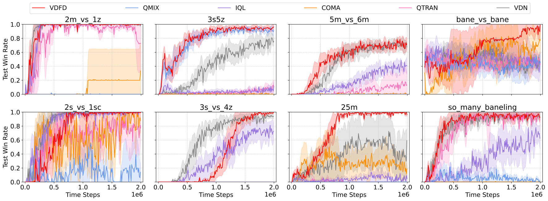
Figure 3: Comparison between the performance of VDFD and the baselines in Hard SMAC environments.

Components of the Learning Objective

We divide the optimization of the overall learning objective into two parts. The first is our decoupled world model, which involves learning imagined data via generative models. The second is our value decomposition framework, which takes as input the agent networks for reinforcement learning.

In the action-conditioned module of the world model, we aim to minimize the KL divergence between the prior and posterior distributions. We need to prevent the prior distribution of $\hat{s}_{t}$ from becoming extremely complex, meaning that we also consider the KL term between the prior and the Normal distribution $p(s_{t}):=\mathcal{N}(0,I)$. Then we obtain:

$$\mathcal{L}_{\text{ac}}^{\text{KL}}(\theta) =\mathcal{D}_{\text{KL}}\left[p^{\text{prior}}_{\theta}\left(\hat{s}_{t}\mid\hat{s}_{t-1},\mathbf{a}_{t-1}\right)\|p(s_{t})\right]$$

$$\phantom{=}\,+\mathcal{D}_{\text{KL}}\left[q_{\theta}(\hat{s}_{t}|\mathbf{h}_{t})\|p^{\text{prior}}_{\theta}\left(\hat{s}_{t}|\hat{s}_{t-1},\mathbf{a}_{t-1}\right)\right]$$

$$=\mathcal{L}_{\text{ac-prior}}^{\text{KL}}(\theta)+\mathcal{L}_{\text{ac-post}}^{\text{KL}}(\theta)$$

Reconstruction processes occur in both generative models. The VAE outputs $\hat{s}_{t-1}^{\prime}$ and $\mathbf{a}_{t-1}^{\prime}$, which are reconstructed from the original past state and actions, $\hat{s}_{t-1}$ and $\mathbf{a}_{t-1}$. Likewise, GALA outputs $\mathbf{h}_{t}^{\prime}$ by reconstructing the authentic past information $\mathbf{h}_{t}$. The reconstruction loss function can be expressed as $\mathcal{L}_{\text{ac}}^{\text{REC}}(\theta)=\mathcal{L}_{\text{ac-prior}}^{\text{REC}}(\theta)+\mathcal{L}_{\text{ac-post}}^{\text{REC}}(\theta)$, where:

$$\mathcal{L}_{\text{ac-prior}}^{\text{REC}}(\theta)=\text{MSE}(\hat{s}_{t-1},\hat{s}_{t-1}^{\prime};\theta)+\text{MSE}(\mathbf{a}_{t-1},\mathbf{a}_{t-1}^{\prime};\theta)$$

$$\mathcal{L}_{\text{ac-post}}^{\text{REC}}(\theta)=\text{MSE}(\mathbf{h}_{t-1},\mathbf{h}_{t-1}^{\prime};\theta)$$

Here $\text{MSE}(\cdot)$ denotes the mean squared error function. The calculation of loss in the action-free branch is very similar to the action-conditioned branch, except that the auto-encoders receive different inputs and produce different outputs. We can derive KL divergence loss and reconstruction loss as:

$$\mathcal{L}_{\text{af}}^{\text{KL}}(\theta) =\mathcal{D}_{\text{KL}}\left[p^{\text{prior}}_{\theta}\left(\hat{v}_{t}\mid\hat{v}_{t-1}\right)\|p(v_{t})\right]$$

$$\phantom{=}\,+\mathcal{D}_{\text{KL}}\left[q_{\theta}(\hat{v}_{t}|\hat{v}_{t-1},\mathbf{z}_{t})\|p^{\text{prior}}_{\theta}\left(\hat{v}_{t}|\hat{v}_{t-1}\right)\right]$$

$$=\mathcal{L}_{\text{af-prior}}^{\text{KL}}(\theta)+\mathcal{L}_{\text{af-post}}^{\text{KL}}(\theta)$$

$$\mathcal{L}_{\text{af}}^{\text{REC}}(\theta) =\text{MSE}(\hat{v}_{t-1},\hat{v}_{t-1}^{\prime};\theta)+$$

$$\phantom{=}\,\text{MSE}((\hat{v}_{t-1},\mathbf{z}_{t-1}),(\hat{v}_{t-1}^{\prime},\mathbf{z}_{t-1}^{\prime});\theta)$$

$$=\mathcal{L}_{\text{af-prior}}^{\text{REC}}(\theta)+\mathcal{L}_{\text{af-post}}^{\text{REC}}(\theta)$$

There is no KL term in the static branch of the world model. The loss is computed as $\mathcal{L}_{\text{st}}(\theta)=\text{MSE}(\hat{\mathbf{z}}_{1:t},\hat{\mathbf{z}}^{\text{static}};\theta)$.

We implement the KL balancing technique as an option when minimizing the KL loss because we want to avoid the posterior representations being regularized towards a poorly trained prior. To address this problem, we employ different learning rates so that the KL divergence is minimized faster with respect to the prior than the posterior. We apply the $stop\_grad(\cdot)$ function in (Hafner et al. 2022), which stops backpropagation from gradients of variables. Let $\alpha\in[0,1]$ be the learning rate. KL balancing can then be defined as:

$$\mathcal{D}_{\text{KLB}}\left[q_{\theta}(\cdot)\|p^{\text{prior}}_{\theta}(\cdot)\right]=\alpha\mathcal{D}_{\text{KL}}\left[q_{\theta}(\cdot)\|{\scriptstyle stop\_grad}(p^{\text{prior}}_{\theta}(\cdot))\right]$$

$$\phantom{=}\,+(1-\alpha)\mathcal{D}_{\text{KL}}\left[{\scriptstyle stop\_grad}(q_{\theta}(\cdot))\|p^{\text{prior}}_{\theta}(\cdot)\right]$$

Finally, we denote the learnable parameters of the value decomposition framework as $\phi$. To maintain consistency with QMIX, we define the TD target and TD loss as:

$$y^{tot}=r_{t}+\gamma\text{max}_{\mathbf{a}_{t+1}}Q_{tot}(\boldsymbol{\tau}_{t+1},\mathbf{a}_{t+1},s_{t+1},;\phi)$$

$$\mathcal{L}^{\text{TD}}(\phi)=\left(y^{tot}-Q_{tot}(\boldsymbol{\tau}_{t},\mathbf{a}_{t},s_{t},;\phi)\right)^{2}$$

The overall loss function of VDFD can thus be expressed as:

$$\mathcal{L}={\scriptstyle\beta_{1}}\mathcal{L}_{\text{ac}}^{\text{KL}}+{\scriptstyle\beta_{2}}\mathcal{L}_{\text{ac}}^{\text{REC}}+{\scriptstyle\beta_{3}}\mathcal{L}_{\text{af}}^{\text{KL}}+{\scriptstyle\beta_{4}}\mathcal{L}_{\text{af}}^{\text{REC}}+{\scriptstyle\beta_{5}}\mathcal{L}_{\text{st}}+\mathcal{L}^{\text{TD}}$$

where $\{\beta_{i}\}_{i\in\{1...5\}}$ are hyper-parameters corresponding to the real-valued masks. By jointly optimizing components of the overall learning objective, we guide VDFD to accurately predict latent trajectories and efficiently perform reinforcement learning, eventually maximizing the returns.

5 Experiments

To assess the performance of VDFD, we consider StarCraft Multi-Agent Challenge (SMAC), a well-established MARL benchmark that consists of battle scenarios corresponding to diverse learning tasks (Samvelyan et al. 2019). We compare our method with widely-applied MARL baselines, including VDN (Sunehag et al. 2017), IQL (Tampuu et al. 2017), COMA (Foerster et al. 2018), QMIX (Rashid et al. 2018), and QTRAN (Son et al. 2019). Moreover, we carry out ablation experiments to analyze the impact of the main components of our method, including different branches in the disentangled world model, the variational graph auto-encoder, and the approximate prior function.

Performance on StarCraft II Micro-Management

Built upon StarCraft II, SMAC focuses on the problem of micro-management, in which each agent takes fine-grained control over an individual unit and selects actions independently. As SMAC requires the official API, we use the newest SC2.4.10 release (Blizzard 2019). It contains stability updates and bug fixes compared to the older releases adopted in previous papers (Rashid et al. 2018; Mahajan et al. 2019; Du et al. 2019; Jeon et al. 2022). Every agent manipulating a unit receives observations only within the unit’s field of view, which leads to partial observability.

Figure 4: Performance of VDFD against the baselines in Easy SMAC environments.

We evaluate the VDFD model on 21 diverse scenarios (maps) to demonstrate its generalization capability. We carry out experiments in each environment with five different seeds and for 2M time steps. The main results are summarized as Test Win Rate, defined as the percentage of episodes in which our army defeats the enemies within the permitted time limit (Samvelyan et al. 2019). We plot the mean and the standard deviation of the five independent runs for each scenario. The SMAC scenarios can be classified into three categories: Easy, Hard, and Super-Hard, based on the difficulty. Figure 4 shows all four Easy environments. VDFD and QMIX are clearly the best performers under this category, almost reaching a win rate of $1.0$. In Figure 3, however, we find there exists a performance gap between Easy and Hard challenges for the baselines. Neither QMIX nor QTRAN shows top performance in more than one of the eight maps. The major reason is that all the Easy scenarios are symmetric, meaning that allies and enemies have the same number of units. However, the Hard challenges have either asymmetric formations or a much larger number of units. The allied army in 25m has 25 Marines, far exceeding 3m and 8m. Asymmetric scenarios, such as so_many_baneling and 2m_vs_1z, require the agents’ effective control over the units to beat the enemies consistently. In 3s_vs_4z, the allied Stalkers need a specific strategy called kiting in order to vanquish the enemy Zealots, which causes delays to the reward.

Figure 5: Performance of VDFD against the other considered algorithms in Super-Hard SMAC environments.

In contrast with the MARL baselines, VDFD achieves the best performance in all of the Hard scenarios, approaching a win rate of $1.0$ in seven of them. It has approximately the same sampling efficiency as VDN in 5m_vs_6m and excels over any other algorithm in the remaining environments. Because VDFD leverages the decoupled world model that performs latent imaginations, it is equipped with useful knowledge about what will happen in the future given different actions. It can therefore maintain precise control over the ally units and adopt the optimal micro-management strategy for a certain environment more easily than other baselines. Furthermore, since VDFD is essentially a model-based approach, it can be more sample-efficient than model-free methods, especially in large-scale battles. This is even more obvious in Figure 5, which indicates that the baselines can hardly learn a policy to defeat the enemy units at any time in Super-Hard maps. By comparison, VDFD demonstrates the highest level of competence in devising winning tactics in all four environments, reaching state-of-the-art performance. The Super-Hard challenges require more effective cooperation and particular micro-management tricks to defeat opponents. In 3s5z_vs_3s6z, the enemy troops have one more Zealot than the allies, which enables them to isolate the ally Zealots from the ally Stalkers and attack the latter. MMM2 is both asymmetric and heterogeneous, in which there are three different types of units on each side. The enemy army in 2c_vs_64zg consists of 64 Zerglings, yielding the largest state and action spaces in SMAC. It is followed by 27m_vs_30m, which consists of 57 Marines in total. Analogous to handling the Hard challenges, the model-based nature of VDFD enables it to reason about the future with reduced sample complexity. Leveraging simulated roll-outs, VDFD is able to learn policies that consistently overcome opponents.

Figure 6: Comparison of VDFD win rates with two sets of ablations on two scenarios 5m_vs_6m and MMM2.

Ablation Studies

We carry out ablation experiments to investigate the effects of the main components in VDFD. First of all, the performance comparison between VDFD and QMIX is implicitly an ablation study that shows the importance of combining the world model with value function factorization.

Secondly, to examine the influence of the modules in the disentangled world model, we perform a set of experiments with three alterations of VDFD: NO-AC, NO-AF, and NO-ST. In Figure 6, we present the ablation results of them. For the first alteration, we remove the action-conditioned branch of the world model by masking out the outputs of the branch. Likewise, NO-AF and NO-ST are implemented to mask out action-free and static branches. It is clear that the lack of any module in the world model results in sub-optimal performance, as they correspond to different parts of the information about the environment dynamics. NO-AC suffers the most because the agent network and the action representations are excluded from the imagination process.

Finally, we conduct an ablation study on the impact of generative models. We consider two variants of VDFD in this ablation study, VDF-SV and VDF-POST. The graph auto-encoder GALA is substituted with a fully-connected VAE for learning the posterior $q_{\theta}(\cdot)$ in VDF-SV. For VDF-POST, we exclude the VAE for learning $p^{\text{prior}}_{\theta}(\cdot)$, which means that only the posterior GALA is used for state inference. Figure 6 reveals that both VDF-SV and VDF-POST are outclassed by VDFD. The former indicates that GALA excels fully-connected VAE in seizing the information about the relationship between agents. The latter implies that it is necessary to approximate the unknown prior, instead of using only the posterior in representation learning.

6 Conclusion

We present VDFD, a model-based method coalescing disentangled representation learning into value function factorization, to address the immense complexity of MARL. To optimize the learning objective, we model the system as Dec-POMDP and integrate generative models in VDFD. We encapsulate the environment representations into a decoupled world model to enhance sample efficiency. VDFD acquires the capability of inferring future states by learning the latent trajectories in the world model. We demonstrate experimentally and analytically that VDFD outstrips well-known MARL baselines and achieves solid generalizability. Using ablation studies, we confirm that the components of VDFD are indispensable for its outstanding performance.

Looking ahead, we aim at implementing different generative models, such as new variants of the VAE, to compare their effectiveness when applied to the world model. Moreover, we plan to explore the applicability of VDFD in difficult sparse-reward environments, which can provide insights into its potential for many real-world applications.

Appendix A Markov Games

In MARL environments, the dynamics of the environment and the reward are determined by the joint actions of all agents, and a generalization of MDP that is able to model the decision-making processes of multiple agents is needed. This generalization is known as stochastic games, also referred to as Markov games (Littman 1994).

Definition A.1

A Markov game $G_{M}$ is defined as a tuple

$$\langle\mathcal{N},\mathcal{S},\{\mathcal{A}^{i}\}_{i\in\{1,...,N\}},P,\{\mathbf{R}^{i}\}_{i\in\{1,...,N\}},\mathit{\gamma}\rangle,where$$

• $\mathcal{N}=\{1,...,N\}$ represents the set of $N$ agents, and it is equivalent to a single-agent MDP when $N=1$.

• $\mathcal{S}$ is the state space of all agents in the environment.

• $\{\mathcal{A}^{i}\}_{i\in\{1,...,N\}}$ stands for the set of action space of every agent $i\in\{1,...,N\}$.

• Define $\mathcal{A}:=\mathcal{A}^{1}\times...\times\mathcal{A}^{N}$ to be the set of all possible joint actions of $N$ agents, and define $\triangle{\mathcal{(S)}}$ to be the probability simplex on $\mathcal{S}$. $P:\mathcal{S}\times\mathcal{A}\to\triangle{\mathcal{(S)}}$ is the probability function that outputs the transition probability to any state $s^{\prime}\in\mathcal{S}$ given state $s\in\mathcal{S}$ and joint actions $\mathbf{a}\in\mathcal{A}$.

• $\{\mathbf{R}^{i}\}_{i\in\{1,...,N\}}$ is the set of reward functions of all agents, in which $\mathbf{R}^{i}:\mathcal{S}\times\mathcal{A}\times\mathcal{S}\to\mathbb{R}$ denotes the reward function of the $i$-th agent that outputs a reward value on a transition from state $s\in\mathcal{S}$ to state $s^{\prime}\in\mathcal{S}$ given the joint actions of all agents $\mathbf{a}\in\mathcal{A}$.

• Lastly, $\mathit{\gamma}\in[0,1]$ represents the discount factor w.r.t. time.

A Markov game, when used to model the learning of multiple agents, makes the interactions between agents explicit. At an arbitrary time step $t$ in the Markov game, an agent $i$ takes its action $a_{i,t}$ at the same time as any other agent given the current state $s_{t}$. The agents’ joint actions, $\mathbf{a}_{t}$, cause the transition to the next state $s_{t+1}\sim P(\cdot|s_{t},\mathbf{a}_{t})$ and make the environment to generate a reward $\mathbf{R}^{i}$ for agent $i$. Every agent has the goal of maximizing its own long-term reward, which can be achieved by finding a behavioral policy

$$\pi(\mathbf{a}|s):=\prod_{i\in\mathcal{N}}\pi^{i}({a^{i}}|s)$$

Specifically, the value function of agent $i$ is defined as

$$V^{i}_{\pi^{i},\pi^{-i}}(s):=\mathbb{E}_{s_{t+1}\sim P(\cdot|s_{t},\mathbf{a}_{t}),a^{-i}\sim\pi^{-i}(\cdot|s_{t})}\big{[}\sum_{t}\gamma^{t}\mathbf{R}^{i}_{t}(s_{t},\mathbf{a}_{t},s_{t+1})|a^{i}_{t}\sim\pi^{i}(\cdot|s_{t}),s_{0}\big{]}$$

where the symbol $-i$ stands for the set of all indices in $\{1,...,N\}$ excluding $i$. It is clear that in a Markov game, the optimal policy of an arbitrary agent $i$ is always affected by not only its own behaviors but also the policies of the other agents. This situation gives rise to significant disparities in the approach to finding solutions between traditional single-agent settings and multi-agent reinforcement learning.

In the realm of MARL, a prevalent situation arises where agents do not have access to the global environmental state. They are only able to make observations of the state by leveraging an observation function. This scenario is formally defined as Dec-POMDP, as we have shown in Definition 3.1. It contains two extra terms for the observation function

$$O(s,i):\mathcal{S}\times\mathcal{N}\to\mathcal{Z}$$

and for the set of observations $\mathcal{Z}$ made by each of the agents, in addition to the definition of the Markov game.

Appendix B Detailed Deduction of the ELBO

Equation 2 in the main paper briefly shows how the ELBO of Dec-POMDP, $\mathcal{L}_{\text{ELBO}}(\mathbf{a}_{0:T},\mathbf{z}_{1:T})$, is derived. We present the full deduction process here.

$$\quad\mathcal{L}_{\text{ELBO}}(\mathbf{a}_{0:T},\mathbf{z}_{1:T})$$

$$=\log p\left(\mathbf{a}_{0:T},\mathbf{z}_{1:T}\right)$$

$$=\log\mathbb{E}_{q_{\theta}(\hat{s}_{1:T}\mid\mathbf{a}_{0:T},\mathbf{z}_{1:T})}\left[\frac{p(\hat{s}_{1:T},\mathbf{a}_{0:T},\mathbf{z}_{1:T})}{q_{\theta}(\hat{s}_{1:T}\mid\mathbf{a}_{0:T},\mathbf{z}_{1:T})}\right]$$

$$\geq\mathbb{E}_{q_{\theta}(\hat{s}_{1:T}\mid\mathbf{a}_{0:T},\mathbf{z}_{1:T})}\log\left[\frac{p(\hat{s}_{1:T},\mathbf{a}_{0:T},\mathbf{z}_{1:T})}{q_{\theta}(\hat{s}_{1:T}\mid\mathbf{a}_{0:T},\mathbf{z}_{1:T})}\right]$$ (3)

$$=\int q_{\theta}(\hat{s}_{1:T}\mid\mathbf{a}_{0:T},\mathbf{z}_{1:T})\log\left[\frac{p(\hat{s}_{1:T},\mathbf{a}_{0:T},\mathbf{z}_{1:T})}{q_{\theta}(\hat{s}_{1:T}\mid\mathbf{a}_{0:T},\mathbf{z}_{1:T})}\right]d\hat{s}_{1:T}$$

$$=\int\sum_{t=1}^{T}q_{\theta}(\hat{s}_{1:T}\mid\mathbf{a}_{0:T},\mathbf{z}_{1:T})\log\left[\frac{p\left(\mathbf{a}_{t}\mid\mathbf{z}_{t}\right)p\left(\mathbf{z}_{t}\mid\hat{s}_{t}\right)p\left(\hat{s}_{t}\mid\hat{s}_{t-1},\mathbf{a}_{t-1}\right)}{q_{\theta}\left(\hat{s}_{t}\mid\hat{s}_{t-1},\mathbf{a}_{t-1},\mathbf{z}_{t}\right)}\right]d\hat{s}_{1:T}$$

$$=\sum_{t=1}^{T}\int q_{\theta}(\hat{s}_{1:t}\mid\mathbf{a}_{0:t},\mathbf{z}_{1:t})\log\left[\frac{p\left(\mathbf{a}_{t}\mid\mathbf{z}_{t}\right)p\left(\mathbf{z}_{t}\mid\hat{s}_{t}\right)p\left(\hat{s}_{t}\mid\hat{s}_{t-1},\mathbf{a}_{t-1}\right)}{q_{\theta}\left(\hat{s}_{t}\mid\hat{s}_{t-1},\mathbf{a}_{t-1},\mathbf{z}_{t}\right)}\right]d\hat{s}_{1:t}$$

$$=\sum_{t=1}^{T}\left\{\int q_{\theta}(\hat{s}_{1:t}\mid\mathbf{a}_{0:t},\mathbf{z}_{1:t})\log\left[p\left(\mathbf{a}_{t}\mid\mathbf{z}_{t}\right)p\left(\mathbf{z}_{t}\mid\hat{s}_{t}\right)\right]d\hat{s}_{1:t}\right.$$

$$\quad\left.+\int q_{\theta}(\hat{s}_{1:t}\mid\mathbf{a}_{0:t},\mathbf{z}_{1:t})\log\left[\frac{p\left(\hat{s}_{t}\mid\hat{s}_{t-1},\mathbf{a}_{t-1}\right)}{q_{\theta}\left(\hat{s}_{t}\mid\hat{s}_{t-1},\mathbf{a}_{t-1},\mathbf{z}_{t}\right)}\right]d\hat{s}_{1:t}\right\}$$

$$=\sum_{t=1}^{T}\left\{\int q_{\theta}(\hat{s}_{1:t}\mid\mathbf{a}_{0:t},\mathbf{z}_{1:t})\log\left[p\left(\mathbf{a}_{t}\mid\mathbf{z}_{t}\right)p\left(\mathbf{z}_{t}\mid\hat{s}_{t}\right)\right]d\hat{s}_{1:t}\right.$$

$$\quad\left.-\int q_{\theta}\left(\hat{s}_{1:t-1}\mid\mathbf{a}_{0:t-1},\mathbf{z}_{1:t-1}\right)\mathcal{D}_{\text{KL}}\left[q_{\theta}\left(\hat{s}_{t}\mid\hat{s}_{t-1},\mathbf{a}_{t-1},\mathbf{z}_{t}\right)\parallel p\left(\hat{s}_{t}\mid\hat{s}_{t-1},\mathbf{a}_{t-1}\right)\right]d\hat{s}_{1:t}\right\}$$

$$=\mathbb{E}_{q_{\theta}\left(\hat{s}_{1:T}\mid\mathbf{a}_{0:T},\mathbf{z}_{1:T}\right)}\sum_{t=1}^{T}\left\{\log\left[p\left(\mathbf{a}_{t}\mid\mathbf{z}_{t}\right)p\left(\mathbf{z}_{t}\mid\hat{s}_{t}\right)\right]\right.$$

$$\left.\quad-\mathcal{D}_{\text{KL}}\left[q_{\theta}\left(\hat{s}_{t}\mid\hat{s}_{t-1},\mathbf{a}_{t-1},\mathbf{z}_{t}\right)\parallel p\left(\hat{s}_{t}\mid\hat{s}_{t-1},\mathbf{a}_{t-1}\right)\right]\right\}$$

$$\approx\sum_{t=1}^{T}\{\log\left[p\left(\mathbf{a}_{t}\mid\mathbf{z}_{t}\right)p\left(\mathbf{z}_{t}\mid\hat{s}_{t}\right)\right]$$

$$\quad-\mathcal{D}_{\text{KL}}\left[q_{\theta}\left(\hat{s}_{t}\mid\hat{s}_{t-1},\mathbf{a}_{t-1},\mathbf{z}_{t}\right)\parallel p\left(\hat{s}_{t}\mid\hat{s}_{t-1},\mathbf{a}_{t-1}\right)\right]\}$$ (4)

$$=\sum_{t=1}^{T}\{\log\left[p\left(\mathbf{a}_{t}\mid\mathbf{z}_{t}\right)\right]+\log\left[p\left(\mathbf{z}_{t}\mid\hat{s}_{t}\right)\right]$$

$$\quad-\mathcal{D}_{\text{KL}}\left[q_{\theta}\left(\hat{s}_{t}\mid\hat{s}_{t-1},\mathbf{a}_{t-1},\mathbf{z}_{t}\right)\parallel p\left(\hat{s}_{t}\mid\hat{s}_{t-1},\mathbf{a}_{t-1}\right)\right]\}$$ (5)

Note that (3) is reached via Jensen’s inequality. Equation 4 can be obtained by sampling $\hat{s}_{1:T}\sim q_{\theta}\left(\hat{s}_{1:T}\mid\mathbf{a}_{0:T},\mathbf{z}_{1:T}\right)$. Equation 5 is identical to Equation 2.

Appendix C Supplemental Related Work

Variational Auto-Encoder (VAE)

The VAE model is a generative model that learns a probability distribution across the input space (Fortuin et al. 2019). It is composed of an encoder network and a decoder network. When provided with the input data $\mathbf{x}$, VAE assumes that $\mathbf{x}$ is generated from a latent variable $\mathbf{z}$ that is not directly observed (Kingma and Welling 2013). The latent variable $\mathbf{z}$ is sampled from the prior distribution over the latent space, which is the centered isotropic multivariate Gaussian $p(\mathbf{z})=\mathcal{N}(\mathbf{z};\boldsymbol{0},\boldsymbol{I})$. The VAE then proceeds to learn the conditional distribution $p(\mathbf{x}|\mathbf{z})$. The posterior distribution of the latent variables, $p(\mathbf{z}|\mathbf{x})$, is assumed to take on an approximate Gaussian with a diagonal covariance to address the intractability of the true posterior distribution. Consequently, the reconstruction error can be computed and back-propagated through the encoder-decoder network (Ha and Schmidhuber 2018).

The encoder of the VAE can be considered as a recognition model, and the decoder serves as a generative model (Kingma and Welling 2013). The VAE model can then be described as the combination of two coupled but independently parameterized models. These two models support each other: the recognition model provides the generative model with the approximates for its posteriors over latent random variables. And conversely, the generative model enables the recognition model to learn informative representations of the data. The recognition model is the approximate inverse of the generative model, according to Bayes’ rule.

Policy Gradient MARL Methods

In single-agent RL, there exists a class of policy gradient methods that do not necessarily require estimates of the value functions. These algorithms update the learning parameters along the direction of the gradient of specific metrics with respect to the policy parameter (Sutton and Barto 2018). The optimal policy is estimated using parametrized function approximations.

Policy gradient algorithms belong to one of the two main categories of MARL algorithms, including actor-critic methods that update policy networks while learning a centralized value function to guide policy optimization based on the policy gradient theorem (Yang and Wang 2020). Gupta, Egorov, and Kochenderfer (2017) described a multi-agent policy gradient version of the trust region policy optimization (Schulman et al. 2015) that enables policy parameter sharing among all agents, but the actor and the critic can only be conditioned on local observations and actions. BiCNet (Peng et al. 2017) also allowed parameter sharing to enhance the scalability of the model, but the communication among agents actually depends on bi-directional RNN. Lowe et al. (2017) adopted the framework of deep deterministic policy gradient (Lillicrap et al. 2015) to multi-agent settings and proposed MADDPG, an approach that uses actors trained on the local observations and a centralized critic for function approximation. The critic is learned by the agents based on their joint observation and joint action. COMA (Foerster et al. 2018) utilized a critic for centralized learning as well, conditioning the critic on the agents’ actions and global state information. The most notable feature of COMA is that the critic computes a counterfactual baseline, to which the estimated return for the joint action is compared. However, COMA tends to suffer high variance in the computation of the counterfactual baseline, causing instabilities in multi-agent benchmarking (Papoudakis et al. 2020). Yu et al. (2021) carefully investigated the performance of proximal policy optimization (Schulman et al. 2017) in cooperative multi-agent environments and obtained competitive sample efficiency with minimal hyperparameter tuning and no major algorithmic modifications. Designing a centrally computed critic to pass the current state information into decentralized agents for learning optimal cooperative behaviors has proved to be an important line of approach in addressing the credit assignment problem (Iqbal and Sha 2018; Du et al. 2019; Zhou et al. 2020).

Value-Based MARL Methods

Another main category of RL algorithms applied to multi-agent systems is value-based methods. Back in the last century, Tan (1997) attempted to use one-step Q-learning (Watkins 1989) on every RL agent in simulated hunter-prey tasks and proposed independent Q-learning (IQL). IQL was later combined with the deep Q-network (Mnih et al. 2015) and extended into learning two-player video games (Tampuu et al. 2017). In a fully decentralized scenario, each agent independently learns an action-value function. It tries to improve its own policy with the assumption of participating in a stationary environment. Because each agent fails to account for the behaviors selected by other agents or the rewards received by them, the assumption of environment stationarity in traditional RL no longer holds (Yang and Wang 2020). There is no theoretical guarantee that an independent learning algorithm will converge in this case (Zhang, Yang, and Başar 2021).

On the other hand, a centralized controller gathers the observation and the joint action of the agents. A method in which all agents have access to global state information and are aware of the non-stationarity in the environment also demonstrates centralization. Boutilier (1996) described the multi-agent Markov decision process, assuming that all agents observe the global rewards. Guestrin, Lagoudakis, and Parr (2002) designed a global payoff function as the sum of local payoff functions, which are a variant of local rewards. The global payoff function was optimized by agents using a variable elimination algorithm. However, due to the combinatorial nature of MARL, the scale of the joint action space will expand exponentially with respect to the number of agents within the same environment (Zhang, Yang, and Başar 2021). As a result, appropriate remedies for scalability issues need to be found.

Recently, studies into MARL have focused on devising algorithms that lie between the two extremes of decentralization (Yang, Borovikov, and Zha 2019; Wang et al. 2020c). They have relaxed the decentralized constraint that state information is always hidden for agents both when they are learning the policies and when they are executing the learned policies. All the agents are now allowed to observe the hidden information only when they are learning, indicating a certain extent of centralization (Kraemer and Banerjee 2016). Building on deep Q-learning agents, the value decomposition network (Sunehag et al. 2017) shares network weights and information channels and specifies roles across them. VDN leverages the joint value function $Q_{tot}$ of the learning agents, which can be additively factorized into individual Q functions $\tilde{Q_{i}}$. The assumption of VDN can be overly restrictive, since the additive value decomposability may not hold for more complex action-value functions. QMIX (Rashid et al. 2018) replaces the full factorization in VDN with the enforcement of monotonicity between the joint $Q_{tot}$ and the individual $\tilde{Q_{i}}$, which enables it to represent a larger class of action-value functions than VDN. The QMIX structure consists of agent networks representing individual value functions, a mixing network estimating $Q_{tot}$, and a set of hyper-networks computing the weights for the mixing network. Realizing that QMIX has difficulties in factorizing tasks with non-monotonic characteristics, Son et al. (2019) developed QTRAN, which creates a transformed function $Q^{\prime}_{jt}$ from any factorizable joint action-value function $Q_{jt}$ and makes sure that the transformed Q function shares the same optimal joint action with the original function. Rigorous research has been conducted in leveraging value function factorization to value-based learning since then (Rashid et al. 2020; Wang et al. 2020b, a; Jeon et al. 2022).

References

- Bai and Jin (2020) Bai, Y.; and Jin, C. 2020. Provable Self-Play Algorithms for Competitive Reinforcement Learning. ArXiv, abs/2002.04017.
- Blizzard (2019) Blizzard. 2019. Blizzard/s2client-proto: StarCraft II client - protocol definitions used to communicate with starcraft II. https://github.com/Blizzard/s2client-proto. Accessed: 2023-08-09.
- Boutilier (1996) Boutilier, C. 1996. Planning, Learning and Coordination in Multiagent Decision Processes. In Proceedings of the 6th Conference on Theoretical Aspects of Rationality and Knowledge, TARK ’96, 195–210. San Francisco, CA, USA: Morgan Kaufmann Publishers Inc. ISBN 1558604179.
- Brafman and Tennenholtz (1999) Brafman, R.; and Tennenholtz, M. 1999. A near-optimal poly-time algorithm for learning in a class of stochastic games. IJCAI International Joint Conference on Artificial Intelligence, 2: 734–739. 16th International Joint Conference on Artificial Intelligence, IJCAI 1999 ; Conference date: 31-07-1999 Through 06-08-1999.
- Brafman and Tennenholtz (2003) Brafman, R.; and Tennenholtz, M. 2003. R-max–A General Polynomial Time Algorithm for Near-Optimal Reinforcement Learning. Journal of Machine Learning Research, 3(2): 213. Publisher: Microtome Publishing.
- Du et al. (2019) Du, Y.; Han, L.; Fang, M.; Liu, J.; Dai, T.; and Tao, D. 2019. LIIR: Learning Individual Intrinsic Reward in Multi-Agent Reinforcement Learning. In Wallach, H.; Larochelle, H.; Beygelzimer, A.; d'Alché-Buc, F.; Fox, E.; and Garnett, R., eds., Advances in Neural Information Processing Systems, volume 32. Curran Associates, Inc.
- Foerster et al. (2018) Foerster, J.; Farquhar, G.; Afouras, T.; Nardelli, N.; and Whiteson, S. 2018. Counterfactual Multi-Agent Policy Gradients. Proceedings of the AAAI Conference on Artificial Intelligence, 32(1). Number: 1.
- Fortuin et al. (2019) Fortuin, V.; Baranchuk, D.; Rätsch, G.; and Mandt, S. 2019. GP-VAE: Deep Probabilistic Time Series Imputation. arXiv e-prints, arXiv:1907.04155.
- Goyal et al. (2021) Goyal, A.; Lamb, A.; Hoffmann, J.; Sodhani, S.; Levine, S.; Bengio, Y.; and Schölkopf, B. 2021. Recurrent Independent Mechanisms. In 9th International Conference on Learning Representations, ICLR 2021, Virtual Event, Austria, May 3-7, 2021. OpenReview.net.
- Guestrin, Lagoudakis, and Parr (2002) Guestrin, C.; Lagoudakis, M. G.; and Parr, R. E. 2002. Coordinated Reinforcement Learning. In International Conference on Machine Learning.
- Gupta, Egorov, and Kochenderfer (2017) Gupta, J.; Egorov, M.; and Kochenderfer, M. J. 2017. Cooperative Multi-agent Control Using Deep Reinforcement Learning. In AAMAS Workshops.
- Ha and Schmidhuber (2018) Ha, D. R.; and Schmidhuber, J. 2018. World Models. ArXiv, abs/1803.10122.
- Hafner et al. (2020) Hafner, D.; Lillicrap, T.; Ba, J.; and Norouzi, M. 2020. Dream to Control: Learning Behaviors by Latent Imagination. arXiv:1912.01603 [cs]. ArXiv: 1912.01603.
- Hafner et al. (2019) Hafner, D.; Lillicrap, T.; Fischer, I.; Villegas, R.; Ha, D.; Lee, H.; and Davidson, J. 2019. Learning Latent Dynamics for Planning from Pixels. arXiv:1811.04551 [cs, stat]. ArXiv: 1811.04551.
- Hafner et al. (2022) Hafner, D.; Lillicrap, T.; Norouzi, M.; and Ba, J. 2022. Mastering Atari with Discrete World Models. ArXiv:2010.02193 [cs, stat].
- Hafner et al. (2023) Hafner, D.; Pasukonis, J.; Ba, J.; and Lillicrap, T. P. 2023. Mastering Diverse Domains through World Models. ArXiv, abs/2301.04104.
- Huang et al. (2020) Huang, S.; Su, H.; Zhu, J.; and Chen, T. 2020. SVQN: Sequential Variational Soft Q-Learning Networks. In International Conference on Learning Representations.
- Iqbal and Sha (2018) Iqbal, S.; and Sha, F. 2018. Actor-Attention-Critic for Multi-Agent Reinforcement Learning. In International Conference on Machine Learning.
- Janner et al. (2019) Janner, M.; Fu, J.; Zhang, M.; and Levine, S. 2019. When to Trust Your Model: Model-Based Policy Optimization. In Wallach, H.; Larochelle, H.; Beygelzimer, A.; d'Alché-Buc, F.; Fox, E.; and Garnett, R., eds., Advances in Neural Information Processing Systems, volume 32. Curran Associates, Inc.
- Jeon et al. (2022) Jeon, J.; Kim, W.; Jung, W.; and Sung, Y. 2022. MASER: Multi-Agent Reinforcement Learning with Subgoals Generated from Experience Replay Buffer. Number: arXiv:2206.10607 arXiv:2206.10607 [cs].
- Kingma and Welling (2013) Kingma, D. P.; and Welling, M. 2013. Auto-Encoding Variational Bayes. arXiv e-prints, arXiv:1312.6114.
- Kipf and Welling (2016) Kipf, T.; and Welling, M. 2016. Semi-Supervised Classification with Graph Convolutional Networks. ArXiv, abs/1609.02907.
- Kok and Vlassis (2006) Kok, J. R.; and Vlassis, N. 2006. Collaborative Multiagent Reinforcement Learning by Payoff Propagation. J. Mach. Learn. Res., 7: 1789–1828.
- Kraemer and Banerjee (2016) Kraemer, L.; and Banerjee, B. 2016. Multi-agent reinforcement learning as a rehearsal for decentralized planning. Neurocomputing, 190: 82–94.
- Lillicrap et al. (2015) Lillicrap, T. P.; Hunt, J. J.; Pritzel, A.; Heess, N. M. O.; Erez, T.; Tassa, Y.; Silver, D.; and Wierstra, D. 2015. Continuous control with deep reinforcement learning. CoRR, abs/1509.02971.
- Littman (1994) Littman, M. L. 1994. Markov Games as a Framework for Multi-Agent Reinforcement Learning. In International Conference on Machine Learning.
- Lowe et al. (2017) Lowe, R.; Wu, Y.; Tamar, A.; Harb, J.; Abbeel, P.; and Mordatch, I. 2017. Multi-Agent Actor-Critic for Mixed Cooperative-Competitive Environments. CoRR, abs/1706.02275.
- Luo et al. (2022) Luo, F.-M.; Xu, T.; Lai, H.; Chen, X.-H.; Zhang, W.; and Yu, Y. 2022. A Survey on Model-based Reinforcement Learning. ArXiv:2206.09328 [cs].
- Mahajan et al. (2019) Mahajan, A.; Rashid, T.; Samvelyan, M.; and Whiteson, S. 2019. MAVEN: Multi-Agent Variational Exploration. In Advances in Neural Information Processing Systems, volume 32. Curran Associates, Inc.
- Mnih et al. (2015) Mnih, V.; Kavukcuoglu, K.; Silver, D.; Rusu, A. A.; Veness, J.; Bellemare, M. G.; Graves, A.; Riedmiller, M.; Fidjeland, A. K.; Ostrovski, G.; Petersen, S.; Beattie, C.; Sadik, A.; Antonoglou, I.; King, H.; Kumaran, D.; Wierstra, D.; Legg, S.; and Hassabis, D. 2015. Human-level control through deep reinforcement learning. Nature, 518(7540): 529–533. Number: 7540 Publisher: Nature Publishing Group.
- Oliehoek and Amato (2016) Oliehoek, F. A.; and Amato, C. 2016. A concise introduction to decentralized POMDPs. Springer.
- Pan et al. (2022) Pan, M.; Zhu, X.; Wang, Y.; and Yang, X. 2022. Iso-Dream: Isolating and Leveraging Noncontrollable Visual Dynamics in World Models. arXiv.org.
- Papoudakis et al. (2020) Papoudakis, G.; Christianos, F.; Schäfer, L.; and Albrecht, S. V. 2020. Benchmarking Multi-Agent Deep Reinforcement Learning Algorithms in Cooperative Tasks. In NeurIPS Datasets and Benchmarks.
- Park et al. (2019) Park, J.; Lee, M.; Chang, H. J.; Lee, K.; and Choi, J. Y. 2019. Symmetric Graph Convolutional Autoencoder for Unsupervised Graph Representation Learning. 2019 IEEE/CVF International Conference on Computer Vision (ICCV), 6518–6527.
- Park, Cho, and Kim (2019) Park, Y. J.; Cho, Y. S.; and Kim, S. B. 2019. Multi-agent reinforcement learning with approximate model learning for competitive games. PLOS ONE, 14(9): 1–20.
- Peng et al. (2017) Peng, P.; Yuan, Q.; Wen, Y.; Yang, Y.; Tang, Z.; Long, H.; and Wang, J. 2017. Multiagent Bidirectionally-Coordinated Nets for Learning to Play StarCraft Combat Games. CoRR, abs/1703.10069.
- Rashid et al. (2020) Rashid, T.; Farquhar, G.; Peng, B.; and Whiteson, S. 2020. Weighted QMIX: Expanding Monotonic Value Function Factorisation. CoRR, abs/2006.10800.
- Rashid et al. (2018) Rashid, T.; Samvelyan, M.; de Witt, C. S.; Farquhar, G.; Foerster, J.; and Whiteson, S. 2018. QMIX: Monotonic Value Function Factorisation for Deep Multi-Agent Reinforcement Learning. ArXiv:1803.11485 [cs, stat].
- Samvelyan et al. (2019) Samvelyan, M.; Rashid, T.; de Witt, C. S.; Farquhar, G.; Nardelli, N.; Rudner, T. G. J.; Hung, C.-M.; Torr, P. H. S.; Foerster, J.; and Whiteson, S. 2019. The StarCraft Multi-Agent Challenge. ArXiv:1902.04043 [cs, stat].
- Schulman et al. (2015) Schulman, J.; Levine, S.; Abbeel, P.; Jordan, M.; and Moritz, P. 2015. Trust Region Policy Optimization. In Bach, F.; and Blei, D., eds., Proceedings of the 32nd International Conference on Machine Learning, volume 37 of Proceedings of Machine Learning Research, 1889–1897. Lille, France: PMLR.
- Schulman et al. (2017) Schulman, J.; Wolski, F.; Dhariwal, P.; Radford, A.; and Klimov, O. 2017. Proximal Policy Optimization Algorithms. ArXiv, abs/1707.06347.
- Shen et al. (2020) Shen, J.; Zhao, H.; Zhang, W.; and Yu, Y. 2020. Model-Based Policy Optimization with Unsupervised Model Adaptation. In Proceedings of the 34th International Conference on Neural Information Processing Systems, NIPS’20. Red Hook, NY, USA: Curran Associates Inc. ISBN 9781713829546.
- Son et al. (2019) Son, K.; Kim, D.; Kang, W. J.; Hostallero, D. E.; and Yi, Y. 2019. QTRAN: Learning to Factorize with Transformation for Cooperative Multi-Agent Reinforcement Learning. In Proceedings of the 36th International Conference on Machine Learning, 5887–5896. PMLR. ISSN: 2640-3498.
- Sunehag et al. (2017) Sunehag, P.; Lever, G.; Gruslys, A.; Czarnecki, W. M.; Zambaldi, V.; Jaderberg, M.; Lanctot, M.; Sonnerat, N.; Leibo, J. Z.; Tuyls, K.; and Graepel, T. 2017. Value-Decomposition Networks For Cooperative Multi-Agent Learning. ArXiv:1706.05296 [cs].
- Sutton and Barto (2018) Sutton, R. S.; and Barto, A. G. 2018. Reinforcement Learning: An Introduction. Cambridge, MA, USA: A Bradford Book. ISBN 0262039249.
- Tampuu et al. (2017) Tampuu, A.; Matiisen, T.; Kodelja, D.; Kuzovkin, I.; Korjus, K.; Aru, J.; Aru, J.; and Vicente, R. 2017. Multiagent cooperation and competition with deep reinforcement learning. PLOS ONE, 12(4): e0172395. Publisher: Public Library of Science.
- Tan (1997) Tan, M. 1997. Multi-Agent Reinforcement Learning: Independent versus Cooperative Agents. In International Conference on Machine Learning.
- Wang et al. (2020a) Wang, J.; Ren, Z.; Liu, T.; Yu, Y.; and Zhang, C. 2020a. QPLEX: Duplex Dueling Multi-Agent Q-Learning. CoRR, abs/2008.01062.
- Wang et al. (2020b) Wang, T.; Dong, H.; Lesser, V.; and Zhang, C. 2020b. ROMA: Multi-Agent Reinforcement Learning with Emergent Roles. In Proceedings of the 37th International Conference on Machine Learning, ICML’20. JMLR.org.
- Wang et al. (2020c) Wang, T.; Gupta, T.; Mahajan, A.; Peng, B.; Whiteson, S.; and Zhang, C. 2020c. RODE: Learning Roles to Decompose Multi-Agent Tasks. CoRR, abs/2010.01523.
- Watkins (1989) Watkins, C. J. C. H. 1989. Learning from delayed rewards. Ph.D. thesis. University of Cambridge.
- Watter et al. (2015) Watter, M.; Springenberg, J.; Boedecker, J.; and Riedmiller, M. 2015. Embed to Control: A Locally Linear Latent Dynamics Model for Control from Raw Images. In Cortes, C.; Lawrence, N.; Lee, D.; Sugiyama, M.; and Garnett, R., eds., Advances in Neural Information Processing Systems, volume 28. Curran Associates, Inc.
- Xu et al. (2018) Xu, H.; Li, Y.; Tian, Y.; Darrell, T.; and Ma, T. 2018. Algorithmic Framework for Model-based Reinforcement Learning with Theoretical Guarantees. ArXiv, abs/1807.03858.
- Yang, Borovikov, and Zha (2019) Yang, J.; Borovikov, I.; and Zha, H. 2019. Hierarchical Cooperative Multi-Agent Reinforcement Learning with Skill Discovery. CoRR, abs/1912.03558.
- Yang and Wang (2020) Yang, Y.; and Wang, J. 2020. An Overview of Multi-Agent Reinforcement Learning from Game Theoretical Perspective. CoRR, abs/2011.00583.
- Yu et al. (2021) Yu, C.; Velu, A.; Vinitsky, E.; Wang, Y.; Bayen, A. M.; and Wu, Y. 2021. The Surprising Effectiveness of MAPPO in Cooperative, Multi-Agent Games. CoRR, abs/2103.01955.
- Zhang et al. (2020) Zhang, K.; Kakade, S.; Basar, T.; and Yang, L. 2020. Model-Based Multi-Agent RL in Zero-Sum Markov Games with Near-Optimal Sample Complexity. In Larochelle, H.; Ranzato, M.; Hadsell, R.; Balcan, M.; and Lin, H., eds., Advances in Neural Information Processing Systems, volume 33, 1166–1178. Curran Associates, Inc.
- Zhang, Yang, and Başar (2021) Zhang, K.; Yang, Z.; and Başar, T. 2021. Multi-Agent Reinforcement Learning: A Selective Overview of Theories and Algorithms. ArXiv:1911.10635 [cs, stat].
- Zhang et al. (2021) Zhang, W.; Wang, X.; Shen, J.; and Zhou, M. 2021. Model-based Multi-agent Policy Optimization with Adaptive Opponent-wise Rollouts. In Zhou, Z.-H., ed., Proceedings of the Thirtieth International Joint Conference on Artificial Intelligence, IJCAI-21, 3384–3391. International Joint Conferences on Artificial Intelligence Organization. Main Track.
- Zhou et al. (2020) Zhou, M.; Liu, Z.; Sui, P.; Li, Y.; and Chung, Y. Y. 2020. Learning Implicit Credit Assignment for Multi-Agent Actor-Critic. ArXiv, abs/2007.02529.