A Comparison between Markov Switching Zero-inflated and Hurdle Models for Spatio-temporal Infectious Disease Counts

Abstract

In epidemiological studies, zero-inflated and hurdle models are commonly used to handle excess zeros in reported infectious disease cases. However, they can not model the persistence (from presence to presence) and reemergence (from absence to presence) of a disease separately. Covariates can sometimes have different effects on the reemergence and persistence of a disease. Recently, a zero-inflated Markov switching negative binomial model was proposed to accommodate this issue. We present a Markov switching negative binomial hurdle model as a competitor of that approach, as hurdle models are often also used as alternatives to zero-inflated models for accommodating excess zeroes. We begin the comparison by inspecting the underlying assumptions made by both models. Hurdle models assume perfect detection of the disease cases while zero-inflated models implicitly assume the case counts can be under-reported, thus we investigate when a negative binomial distribution can approximate the true distribution of reported counts. A comparison of the fit of the two types of Markov switching models is undertaken on chikungunya cases across the neighborhoods of Rio de Janeiro. We find that, among the fitted models, the Markov switching negative binomial zero-inflated model produces the best predictions and both Markov switching models produce remarkably better predictions than more traditional negative binomial hurdle and zero-inflated models.

Keywords : Bayesian inference; Endemic-epidemic model; Under-reporting; Chikungunya

1 Introduction

In epidemiological studies, disease counts taken at different spatial locations across different instants in time often contain a great number of zeros. In this case, a count distribution, like the Poisson or Negative Binomial distribution, is often unable to capture the large number of observed zero counts present in the data. Zero-inflated (ZI) and hurdle models [RN7, RN8] are the two primary types of models that have been proposed to deal with count data with excess zeros.

The first paper on ZI Poisson (ZIP) regression models handled count data with excess zeros by mixing a Poisson distribution and a distribution with a point mass at zero. [RN6] In practice, due to the need for model flexibility, we can mix count distributions other than the Poisson with a distribution that has point mass at zero, like a ZI negative binomial model (ZINB) [RN46]. Overall, we refer to them as ZI count (ZIC) models [RN2]. In an epidemiology application of a ZIC model, a Bernoulli process is used to determine whether the disease is present [RN49]. A one from the Bernoulli process indicates the disease is present and the number of cases comes from the count process, while a zero indicates the disease is absent and the number of cases is zero. Zeros can come from the zero mass process or the count process. Correspondingly, zero counts produced by a ZI model are often distinguished by "structural zeros", from the zero mass process that corresponds to the absence of disease, and "sampling zeros", which imply unreported cases from the at-risk population during the study period, produced by the count process [RN1]. We can also relate associated factors to the Bernoulli process, which controls the presence/absence of the disease [RN9].

In comparison with ZI models, hurdle models also consist of two mixed parts: one is a zero-generating process, but the other part is a zero truncated count process, like a zero-truncated negative binomial distribution, which leads to a negative binomial hurdle model (NBH) [RN50]. We can associate certain factors with the probability of observing a positive count in the same way as ZI models [RN12]. However, unlike ZI models, in hurdle models zeros can not be produced by the at-risk population. Namely, in hurdle models, all zero counts are "structural zeros" by construction. Therefore, compared to ZI models, a zero in a hurdle model, within an epidemiological context, can only arise due to the actual absence of the disease rather than the undetected situation. Implicitly, this means that the disease is perfectly detected or that undetected cases are too few to be relevant, which is the main difference in the interpretation of zeros between ZI and hurdle models.

Under-reporting is another challenge for researchers in epidemiology, where the reported disease counts can be less than the true counts. A zero-truncated count process, like a zero-truncated negative binomial distribution, can be applied to the reported counts when the disease is present under the perfect detection assumption of a hurdle model. However, a count distribution, such as the negative binomial or Poisson, can fail to approximate the true distribution of reported cases under the imperfect detection assumption of a ZI model. Section 2 explores when the approximation can be acceptable.

Under the framework of spatio-temporal data, we can separate the presence of the disease into two categories, persistence (from presence to presence) and reemergence (from absence to presence). ZI models can only accommodate the characteristics of overall disease presence and cannot model reemergence and persistence separately. Sometimes, covariate effects can be quite different between the reemergence and persistence of an infectious disease [RN5]. A recent paper extended the common zero-inflated count model (ZIC) to a zero-state coupled Markov switching negative binomial model (ZS-CMSNB), under which the disease switched between periods of presence and absence in each area through a series of Markov chains where the reemergence and persistence were modelled separately [RN5]. As a counterpart to the ZI models, in our framework, we follow the structure of hurdle models to assume that the zero mass process represents the reported cases when the disease is absent and a truncated count distribution (e.g. a zero truncated negative binomial distribution) represents the reported cases when the disease is present. We then assume a non-homogeneous Markov Chain switches the disease between the presence and absence states. We compare the Markov-switching negative binomial hurdle model to its zero-inflated counterpart on the fit, plausibility of assumptions and interpretation when modelling weekly chikungunya reported cases in Rio de Janeiro. In [RN1] they compared hurdle and zero-inflated models but not specifically in an epidemiological context or with Markov switching models.

1.1 Motivating example: Chikungunya cases in Rio de Janeiro

Chikungunya is an infectious disease that became endemic in Rio de Janeiro, Brazil in 2016 [RN30]. For our study, we obtained publicly available data from the website of the Municipal Health Secretariat of Rio de Janeiro. The data comprises weekly counts across the 160 administrative districts of Rio de Janeiro. The data spans the period between January 2015 and May 2022. It is suspected that chikungunya started circulating unnoticed in the city before the first reported transmission [RN31]. Due to a lack of social index information, we decide to exclude one small district, Paquetá Island.

Figure 1 illustrates weekly chikungunya infectious cases for two administrative districts of Rio de Janeiro, one with a small population (Saúde) and the other one (Campo Grande) relatively large. In the Saúde district, chikungunya is only observed present for a couple of weeks and is observed absent for most of the period (96.61% of the study period). In the Campo Grande district, the disease showed a longer time of observed persistence (54.95% of the study period) and is observed to reemerge (go from absence to presence) quicker. These differences in chikungunya persistence and reemergence probabilities at the district level could be explained by population differences, as there is a well-known inverse relationship between population and the rate of disease extinction in epidemiology [RN27]. Socioeconomic factors may also partly explain the distinct patterns [RN28], since districts with lower Human Development Index (HDI) tend to lack tap water supply, which allows mosquitoes to breed in water storage containers and transmit disease [RN35]. Because the mosquitoes are accustomed to urban utilities, the level of which is inversely correlated with the proportion of green areas (areas with agriculture, swamps and shoals, tree and shrub cover, and woody-grass cover) [RN47], the level of green area in a district could be inversely correlated with the disease transmission there. In this motivating example, we are mainly interested in investigating associations between certain factors, such as HDI and green areas, and Zika emergence and persistence, as well as the problem of future case prediction in a district to help policymakers better direct resources to districts in need.

This paper is organized as follows. In Section 2, we explore mathematically how differences in hurdle and ZI model structures are related implicitly to assumptions about disease detection. In Section 3 we review the statistical models and propose a Markov switching hurdle model. Section 4 introduces the inferential procedure for model fitting and temporal prediction. Section 5 presents the analysis of the chikungunya data and a comparison in terms of prediction between the hurdle and zero-inflated Markov switching models, and also more conventional zero-inflated and hurdle alternatives. The paper concludes with a discussion in Section LABEL:sec:_discussion.

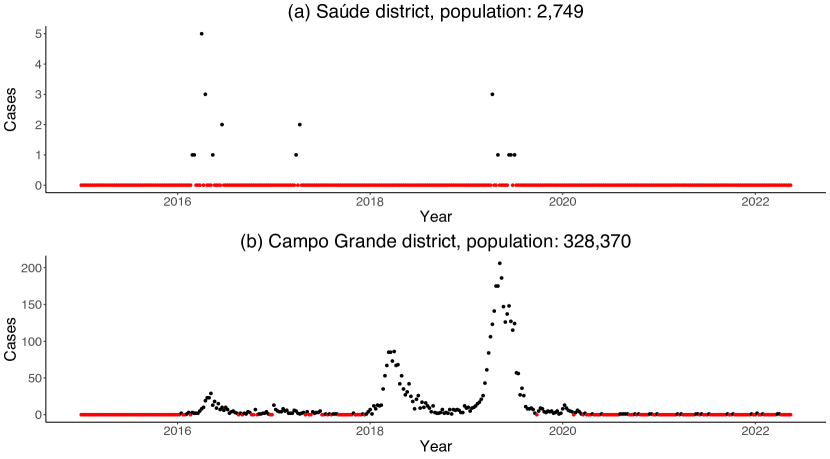
Figure 1: Weekly chikungunya infectious cases for (a) Saúde district and (b) Campo Grande district; red solid circles represent 0 cases at the reported week during the study period.

2 A Negative Binomial Approximation of Under-reported Case Counts

In epidemiology, both ZI and hurdle models assume that, for every area and/or time period, the disease can be either present or absent and that when the disease is absent no cases will be reported [RN45, harris_climate_2019]. The main difference between hurdle and ZI models is that, when the disease is present, a hurdle model assumes the reported cases come from a zero-truncated distribution while a ZI model assumes the reported cases are generated by a count distribution that can produce zeroes, such as the negative binomial distribution. To illustrate how these differences relate to assumptions about disease detection, let $Z$ be the actual counts when the disease is present and $Y$ be the reported counts when the disease is present. When the disease is present the actual counts $Z$ must be greater than zero and so we can assume $Z$ follows a zero-truncated negative binomial model, that is,

$$Z|\lambda,r\sim ZTNB(\lambda,r),$$ (1)

where $\lambda$ is the mean value and $r$ is the over-dispersion parameter of the negative binomial that gets truncated assuming the variance of the negative binomial that gets truncated is given by $\lambda+\lambda^{2}/r$. We can then assume the reported counts $Y$ given the actual counts $Z$ follows a binomial distribution, i.e.,

$$Y|Z,p_{0}\sim BIN(Z,p_{0}),$$ (2)

where $p_{0}$ is the probability of reporting any one count when the disease is present. It can be shown that the marginal distribution of $Y$ is,

$$P(Y=y|\lambda,r,p_{0})=\mathopen{}\mathclose{{}\left\{\begin{array}[]{lcclcc}\frac{(\frac{r}{r+\lambda})^{r}p_{0}^{y}(r+y-1)!(\frac{\lambda}{\lambda+r})^{y}(\frac{\lambda p_{0}+r}{\lambda+r})^{-r-y}}{(r-1)!y!(1-(\frac{r}{r+\lambda})^{r})}&&&\ y>0,&&\\ \frac{(\frac{r}{\lambda})^{r}(1-(\frac{\lambda p_{0}+r}{\lambda+r})^{-r})}{(\frac{r}{\lambda})^{r}-(\frac{\lambda+r}{\lambda})^{r}}&&&\ y=0.&&\end{array}}\right.$$ (3)

See Supplementary Material (SM) Section 1 for the derivation of this distribution.

Under perfect detection $p_{0}=1$ and $Y=Z$ leading to a hurdle model with count part given by (1). If instead $p_{0}<1$ zeroes could arise when the disease is present if it goes undetected leading to a ZI model with count part given by (3). However, in practice, we cannot use (3) as the count part of a ZI model since typically the reporting probability $p_{0}$ is not identifiable from the reported cases alone [RN51]. Usually, a negative binomial distributed variable $W$ is used as the count part of a ZI model and, therefore, the distribution of $W$ would be implicitly approximating the distribution of true reported counts $Y$[RN55]. To test the appropriateness of this approximation we can match the mean and variance of $W$ with the exact distribution (3),

$$W\sim NB(\mu^{(w)},r^{(w)}),$$ (4)

where $\mu^{(w)}=\frac{p_{0}\lambda}{1-(\frac{r}{r+\lambda})^{r}}$ and $r^{(w)}=\frac{1}{(1-(\frac{r}{r+\lambda})^{r})(1+\frac{1}{r})-1}$. See SM Section 1 for this derivation.

Figure 2 shows three scenarios of the comparison between the exact distribution (3) and the approximated negative binomial distribution (4) of the reported counts. When the reporting rate is small, using a negative binomial distribution is close to the exact distribution of the reported counts. This indicates that a ZI model with the commonly used negative binomial count part is a reasonable choice under a small reporting rate. However, the approximation does not work well when the reporting rate gets large. This suggests a hurdle model may be more applicable under a large reporting rate as the hurdle model assumes $p_{0}=1$. Note that this result is intuitive since if the reporting rate is very large we would not expect many zeroes due to a failure to detect the disease even if the expected number of actual cases were small. The negative binomial distribution places a lot of weight at 0 when the mean is small and thus it would not fit the true reported cases well.

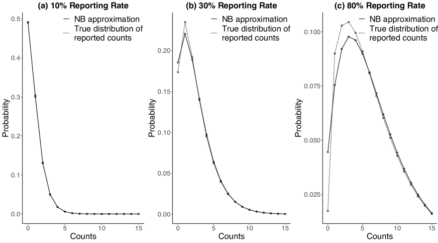
Figure 2: Probability mass functions of the true distribution of reported counts ($Y$) and the approximated NB distribution ($W$) under (a) a low reporting rate ($p_{0}=0.1$), (b) a moderate reporting rate ($p_{0}=0.3$) and (c) a large reporting rate ($p_{0}=0.8$). The over-dispersion of the actual counts ($r=2$) and the incidence of actual cases ($\lambda=8$) are the same for all three scenarios.

In this section, we discussed the marginal distribution of reported counts under imperfect detection and when a negative binomial distribution approximates it closely. In Section 3 we will show expressions for hurdle models with zero-truncated negative binomial count parts, and ZI models with negative binomial count parts as a possibly reasonable approximating distribution of the true reported counts. Following the mean and variance of the distribution of the counts in equation (3), we allow the mean and the over-dispersion parameters of the negative binomial distribution to depend on covariates. In Section 5 we will produce a real analysis of the chikungunya infectious data, and we also allow the mean and over-dispersion parameter of the negative binomial distribution to depend on a vector of selected covariates.

3 Modeling Zeros: Zero-inflated and Hurdle Models

Assume we have infectious disease cases in areas $i=1,2,...,N$ and at times $t=1,2,...,T$. Let $y_{it}$ be the reported disease case counts from area $i$ at time $t$. Let $X_{it}$ be a binary random variable that indicates the true presence or absence of the disease in area $i$ at time $t$, i.e., $X_{it}=1$ if the disease is present and $X_{it}=0$ if the disease is absent. Additionally, let $\bm{y}^{(t-1)}=(\bm{y}_{1},\bm{y}_{2},\cdots,\bm{y}_{t-1})^{T}$ be the vector of counts up to time $t-1$. Each component of $\bm{y}^{({t-1})}$, say at time $k$, defined as $\bm{y}_{k}=(y_{1k},y_{2k},\cdots,y_{Nk})^{T}$, is the vector containing the observed counts of the disease across the areas at time $k$, $k=1,2,\cdots,t-1$. Finally, all available observations are stacked onto the vector $\bm{y}=(\bm{y}_{1},\bm{y}_{2},\cdots,\bm{y}_{T})^{T}$.

Under the assumptions of a zero-inflated or hurdle model, when the disease is present the reported cases are generated by a count distribution, say $p(y_{it}\mid\bm{\theta}_{it})$ and when the disease is absent no cases are reported. Note that $\bm{\theta}_{it}$ is the parameter vector defining the distribution of $Y_{it}$. Generally, the reported cases for area $i$ at time $t$ given the disease’s presence/absence status and the vector of counts up to time $t$ can be expressed as

$$Y_{it}|X_{it},\bm{y}^{(t-1)}\sim\mathopen{}\mathclose{{}\left\{\begin{array}[]{lcc}0&\ \text{if}\ X_{it}=0&(\text{absence}),\\ p(y_{it}\mid\bm{\theta}_{it})&\ \text{if}\ X_{it}=1&(\text{presence}).\end{array}}\right.$$ (5)

As discussed in Section 2, a negative binomial distribution is a reasonable specification for $p(y_{it}\mid\bm{\theta}_{it})$ if the reporting rate is small. Then a zero that comes from the negative binomial distribution represents the disease going undetected while a zero from the zero mass distribution represents the true absence of the disease. Such models are known as zero-inflated models [RN45]. In contrast to zero-inflated models, if we assume perfect detection of the disease, we can specify $p(y_{it}\mid\bm{\theta}_{it})$ as a zero-truncated negative binomial distribution since, under perfect detection, there will always be cases reported when the disease is present. Such models are known as hurdle models [harris_climate_2019].

The practical difference between ZI and hurdle models is that for ZI models, the zeros can come from both disease absence or undetected cases while in hurdle models zero counts can only be generated due to the actual absence of the disease. That is, hurdle models assume perfect detection of the cases or at least that undetected cases are too few to be relevant. However, a zero-inflated model allows for the imperfect detection of disease cases.

3.1 Modeling the Presence/Absence of Disease

If the disease is present or absent, we would expect it to be more likely to be present or absent again in the next reported time. Therefore, we assume that $X_{it}$, conditioned on all the previous cases before time $t$, $\bm{y}^{(t-1)}$, and the presence/absence of the disease in all neighboring areas in the previous time, denoted by $\bm{X}_{(-i)(t-1)}$, follows a two-state non-homogeneous Markov chain. The transition probability matrix of the Markov chain is denoted by,

$$\Gamma\mathopen{}\mathclose{{}\left(X_{it}|\bm{y}^{(t-1)},\bm{X}_{(-i)(t-1)}}\right)=\hbox{}\vbox{\kern 0.86108pt\hbox{$\kern 0.0pt\kern 2.5pt\kern-2.0pt\mathopen{}\mathclose{{}\left[\kern 0.0pt\kern-2.5pt\kern-5.55557pt\vbox{\kern-0.86108pt\vbox{\vbox{ \halign{\kern\arraycolsep\hfil\@arstrut$\kbcolstyle#$\hfil\kern\arraycolsep& \kern\arraycolsep\hfil$\@kbrowstyle#$\ifkbalignright\relax\else\hfil\fi\kern\arraycolsep&& \kern\arraycolsep\hfil$\@kbrowstyle#$\ifkbalignright\relax\else\hfil\fi\kern\arraycolsep\cr 2.0pt\hfil\@arstrut$\scriptstyle\textbf{State}$\hfil\kern 2.0pt&2.0pt\hfil$\scriptstyle X_{it}=0\ (\textbf{absence})\,$\hfil\kern 2.0pt&2.0pt\hfil$\scriptstyle$\hfil\kern 2.0pt&2.0pt\hfil$\scriptstyle X_{it}=1\ (\textbf{presence})\,\\[8pt]X_{i,t-1}=0\ (\textbf{absence})\,$\hfil\kern 2.0pt&2.0pt\hfil$\scriptstyle 1-p01_{it}$\hfil\kern 2.0pt&2.0pt\hfil$\scriptstyle$\hfil\kern 2.0pt&2.0pt\hfil$\scriptstyle p01_{it}\\[5pt]X_{i,t-1}=1\ (\textbf{presence})\,$\hfil\kern 2.0pt&2.0pt\hfil$\scriptstyle 1-p11_{it}$\hfil\kern 2.0pt&2.0pt\hfil$\scriptstyle$\hfil\kern 2.0pt&2.0pt\hfil$\scriptstyle p11_{it}$\hfil\kern 2.0pt\crcr}}}}}\right]$}},$$ (7)

where

$$p01_{it}=P(X_{it}=1|X_{i,t-1}=0,\bm{y}^{(t-1)},\bm{X}_{(-i)(t-1)})\quad\text{(probability of reemergence)},$$

$$p11_{it}=P(X_{it}=1|X_{i,t-1}=1,\bm{y}^{(t-1)},\bm{X}_{(-i)(t-1)})\quad\text{(probability of persistence)}.$$

We also want a statistical model able to investigate how disease persistence and reemergence may be explained by multiple risk factors. Due to the characteristics of infectious diseases, the disease is more likely to be present in an area when the disease is present in its neighboring areas in the previous week. Therefore, the probability of reemergence in area $i$ at time $t$, i.e. $p01_{it}$, can depend on a vector of risk factors $\bm{g}_{it}$ and the spatial neighbors as

$$\text{logit}(p01_{it})=\alpha_{0}^{(0)}+\bm{g}_{it}^{T}\bm{\alpha}^{(0)}+\gamma_{1}\sum_{j\in\text{Nei}(i)}X_{j,t-1},$$ (8)

where $\text{Nei}(i)$ represents the index set of all neighboring areas of area $i$, and $\bm{g}_{it}=(g_{it}^{(1)},g_{it}^{(2)},\cdots,g_{it}^{(D)})^{T}$ is a D-dimensional covariate vector. Similarly, the probability of persistence in area $i$ at time $t$, i.e. $p11_{it}$ is modelled as

$$\text{logit}(p11_{it})=\alpha_{0}^{(1)}+\delta^{(1)}\log(y_{i,t-1}+1)+\bm{g}_{it}^{T}\bm{\alpha}^{(1)}+\gamma_{2}\sum_{j\in\text{Nei}(i)}X_{j,t-1},$$ (9)

where $\log(y_{i,t-1}+1)$ is a term representing the reported case counts for area $i$ at time $t-1$. The term $\log(y_{i,t-1}+1)$ is included in the model for $p11_{it}$ because we find it reasonable to assume that the disease will be less likely to go extinct if there are many cases previously. In (8) and (9), $\bm{\alpha}^{(0)}$ and $\bm{\alpha}^{(1)}$ represent the effects of the covariates on the disease’s reemergence and persistence probabilities respectively, and they can be different. Note that this is different from more classical zero-inflated and hurdle models where $\bm{\alpha}^{(0)}=\bm{\alpha}^{(1)}=\bm{\alpha}$ and $\alpha_{0}^{(0)}=\alpha_{0}^{(1)}=\alpha_{0}$, which implicitly assumes each covariate must have the same effect on the reemergence and persistence of the disease[RN56]. For the Markov chain, we also need to set initial state distributions for the first time in each area, which we denote by $p_{0}(X_{i0})$ for $i=1,2,...,N$.

Modelling the parameters of the count part

It is assumed that $p(y_{it}\mid\bm{\theta}_{it})$ in equation (5) follows either a negative binomial distribution, in the case of the ZI models, or a truncated negative binomial distribution, in the case of the hurdle models, with mean $\mu_{it}$ and overdispersion parameter $r_{it}$ (for the ZTNB $\mu_{it}$ and $r_{it}$ are the mean and overdispersion parameter of the NB that gets truncated).

For infectious disease counts, previous cases are likely to transmit the disease to other individuals, creating new cases; that is, for an area $i$, the previously reported cases, i.e. $y_{i,t-1}$, may affect the expected value $\mu_{it}$ of the reported cases $y_{it}$. Thus, we decompose $\mu_{it}$ as in Bauer and Wakefield (2018) [RN29], that is,

$$\mu_{it}=\mu_{it}^{AR}y_{i,t-1}+\mu_{it}^{EN},$$ (10)

where $\mu_{it}^{AR}$ is the autoregressive rate which is a multiplier on the previous week’s cases that is meant to capture transmission from the previous cases and $\mu_{it}^{EN}$ is an endemic component meant to capture infectious risk from other sources like the environment and imported cases.

The autoregressive AR rate $\mu_{it}^{AR}$ is modelled as

$$\mu_{it}^{AR}=\exp{(b0_{i}+\bm{g}_{it}^{T}\bm{\beta}^{AR})},$$ (11)

where $b0_{i}|\sigma_{b0}^{2}\sim_{IID}N(\beta_{0}^{AR},\sigma_{b0}^{2})$ is an area level random effect and $\bm{\beta}^{AR}$ represents the possible effects of risk factors $\bm{g}_{it}$ on $\mu_{it}^{AR}$. The endemic part $\mu_{it}^{EN}$ is modelled as

$$\mu_{it}^{EN}=\exp{\mathopen{}\mathclose{{}\left(b_{i}+\beta_{2}^{EN}sin\mathopen{}\mathclose{{}\left(\frac{t}{52}2\pi}\right)+\beta_{3}^{EN}cos\mathopen{}\mathclose{{}\left(\frac{t}{52}2\pi}\right)}\right)},$$ (12)

where $b_{i}|\sigma_{b}^{2}\sim_{IID}N(\beta_{0}^{EN}+\beta_{1}^{EN}log(N_{i}),\sigma_{b}^{2})$ is an areal level random effect whose mean is a linear function of the population size of the $i$th district. A possible annual seasonal component is modelled by the sine and cosine components [RN34]. It is known that environmental variables such as temperature and precipitation impact the life cycle of the mosquito that transmits chikungunya [RN41]. As we did not have access to these environmental variables in Rio de Janeiro, we include sine/cosine components as a surrogate to account for the seasonal structure that might be present in the data. We expect there to be more reported cases in the summer than in the winter by the strong effects of climate variables on the mosquito’s life cycle [RN32].

As shown in Equation (4) the overdispersion parameter of the negative binomial approximation to the true reported counts depends on the expected number of actual counts and so should vary across space and time with covariates. Therefore, we model the overdispersion parameter of the NB and ZTNB distributions, $r_{it}$, as a log-linear function of covariates and past cases,

$$\log(r_{it})=\alpha_{0}^{(2)}+\bm{g}_{it}^{T}\bm{\alpha}^{(2)}+\delta^{(2)}log(y_{i,t-1}+1).$$ (13)

In this paper, we will refer to the models defined by the following equations:

• ZINB: Equations (5) with $p(y_{it}|\bm{\theta}_{it})=NB(\mu_{it},r_{it})$; (7)-(9) with $\bm{\alpha}^{(0)}=\bm{\alpha}^{(1)}=\bm{\alpha}$, $\alpha_{0}^{(0)}=\alpha_{0}^{(1)}=\alpha_{0}$ and $\gamma_{1}=\gamma_{2}=0$; (10)-(13),

• NBH: Equations (5) with $p(y_{it}|\bm{\theta}_{it})$ following a zero truncated negative binomial distribution, that is, $p(y_{it}|\bm{\theta}_{it})=ZTNB(\mu_{it},r_{it})$; (7)-(9) with $\bm{\alpha}^{(0)}=\bm{\alpha}^{(1)}=\bm{\alpha}$, $\alpha_{0}^{(0)}=\alpha_{0}^{(1)}=\alpha_{0}$ and $\gamma_{1}=\gamma_{2}=0$; (10)-(13),

• ZS-MSNB (Zero-state Markov switching negative binomial) [RN5]: Equations (5) with $p(y_{it}|\bm{\theta}_{it})=NB(\mu_{it},r_{it})$, (7)-(13),

• ZS-MSNBH (Proposed zero-state Markov switching negative binomial hurdle): Equations (5) with $p(y_{it}|\bm{\theta}_{it})=ZTNB(\mu_{it},r_{it})$, (7)-(13).

The ZINB and NBH models represent classical commonly fit versions of ZI and hurdle models [RN1, tawiah_zero-inflated_2021] while the ZS-MSNB and ZS-MSNBH models represent their Markov switching counterparts. The Markov switching models have some important advantages including allowing for separate covariate effects between the reemergence and persistence and being able to more easily account for many consecutive 0s and positive counts since when the disease is in the presence or absence states it is usually more likely to remain there due to the Markov chain [RN5].

There are some similarities between the specifications of the ZS-MSNB and ZS-MSNBH models. For a specific number of reported cases in district $i$ at time $t$, $y_{it}$, they both assume a latent indicator variable $X_{it}$ to distinguish the case-generating process. However, the indicator variable $X_{it}$ in a ZS-MSNB model is assumed to be not observed when there are zero reported cases[RN49], because in the ZS-MSNB model, both the negative binomial process and the zero process can produce a zero count, which means an observed zero count could be due to either the disease being absent or undetected. These differences in the model specification of $y_{it}|X_{it}$ lead to divergent interpretations. The ZS-MSNBH model assumes perfect detection of the counts, while the ZS-MSNB model allows for the imperfect detection of the disease counts.

Furthermore, ZS-MSNB and ZS-MSNBH are a priori plausible in different patterns of case data. When a time series shows switching between long periods of only zero counts and long periods of positive counts, interspersed with some zeros, a ZS-MSNB model is more applicable, like the time series of reported cases shown in Figure 1(b). In contrast, for the case where a time series shows switching between long periods of zero counts and long periods of only positive counts, a ZS-MSNBH model may fit better than a ZS-MSNB model.

4 Inferential Procedure

Let $\bm{X}=(\bm{X}_{1},\bm{X}_{2},...,\bm{X}_{T})^{T}$ be the vector of all state indicators, where $\bm{X}_{t}=(X_{1t},X_{2t},...,X_{Nt})^{T}$. Let $\bm{\Theta}_{0}=(\beta_{0}^{AR},\bm{\beta}^{AR},\beta_{2}^{EN},\beta_{3}^{EN},\beta_{0}^{EN},\beta_{1}^{EN},\alpha_{0}^{(0)},\alpha_{0}^{(1)},\alpha_{0}^{(2)},\bm{\alpha}^{(0)},\bm{\alpha}^{(1)},\bm{\alpha}^{(2)},\delta^{(1)},\delta^{(2)},\gamma_{1},\gamma_{2},\sigma_{b},\sigma_{b0},\\\{b_{i}\}_{i=1}^{N},\{b0_{i}\}_{i=1}^{N})^{T}$ be the whole parameter vector apart from state indicators $\bm{X}$.

In a ZS-MSNBH model, the marginal likelihood function given $\bm{y}$, marginalizing out the state indicators, is given by

$$p(\bm{y}|\bm{\Theta}_{0}) =\prod_{i=1}^{N}\prod_{t=2}^{T}p(y_{it}|\bm{y}^{(t-1)},\bm{\Theta}_{0})$$ (14)

$$=\prod_{i=1}^{N}\prod_{t=2}^{T}\text{ZTNB}(y_{it}|\mu_{it},r_{it})p01_{it}^{1-I[y_{i,t-1}>0]}p11_{it}^{I[y_{i,t-1}>0]}+$$

$$I[y_{it}=0](1-p01_{it})^{1-I[y_{i,t-1}>0]}(1-p11_{it})^{I[y_{i,t-1}>0]},$$

where $I[\mathchoice{\mathbin{\vbox{\hbox{\scalebox{0.5}{$\displaystyle\bullet$}}}}}{\mathbin{\vbox{\hbox{\scalebox{0.5}{$\textstyle\bullet$}}}}}{\mathbin{\vbox{\hbox{\scalebox{0.5}{$\scriptstyle\bullet$}}}}}{\mathbin{\vbox{\hbox{\scalebox{0.5}{$\scriptscriptstyle\bullet$}}}}}]$ represents an indicator function and $\text{ZTNB}(y_{it}|\mu_{it},r_{it})$ represents a zero-truncated negative binomial distribution where the mean and over-dispersion parameters of the associated negative binomial are given by $\mu_{it}$ and $r_{it}$ respectively. We follow the Bayesian paradigm to estimate the parameters of the models. One of the reasons for using the Bayesian approach is because we cannot marginalize out $\bm{X}$ in the ZS-MSNB model, and so it is the only tractable method for that model [RN5]. We assume prior independence among the components of $\bm{\Theta}_{0}$. Then we specify normal priors for $\bm{\beta}^{AR}$, $\beta_{2}^{EN}$, $\beta_{3}^{EN}$, $\beta_{0}^{EN}$, $\beta_{1}^{EN}$, $\alpha_{0}^{(0)}$, $\alpha_{0}^{(1)}$, $\alpha_{0}^{(2)}$, $\bm{\alpha}^{(0)}$, $\bm{\alpha}^{(1)}$, $\bm{\alpha}^{(2)}$, $\delta^{(1)}$, $\delta^{(2)}$, $\gamma_{1}$ and $\gamma_{2}$ ; inverse gamma priors for $\sigma^{2}_{b0}$ and uniform prior for $\sigma_{b}$. Regardless of the prior specification, the posterior distribution is not available in closed form. Thus, we will use Markov chain Monte Carlo methods, particularly a Gibbs sampler with some steps of the Metropolis-Hastings algorithm, to draw samples from the resultant posterior distribution.

In a ZS-MSNB model, the joint likelihood function considering $\bm{X}$ and $\bm{y}$ is given by

$$p(\bm{y},\bm{X}|\bm{\Theta}_{0})=\prod_{i=1}^{N}\prod_{t=2}^{T}p(y_{it}|X_{it},\bm{y}^{(t-1)},\bm{\Theta}_{0})\prod_{i=1}^{N}p(X_{i1})\prod_{t=2}^{T}p(X_{it}|\bm{X}_{t-1},\bm{y}^{(t-1)},\bm{\Theta}_{0}).$$ (15)

The Gibbs sampler procedure for the ZS-MSNB model is challenging as $\bm{X}$ is not fully observed and $\bm{X}$ cannot be marginalized from the likelihood function, we follow a data augmentation algorithm to obtain samples from the posterior distribution of this model [RN5].

4.1 Model Comparison Criteria and Temporal Prediction

In our Bayesian framework, we can use the Watanabe-Akaike information criterion (WAIC) [RN14] to compare some model specifications. For a ZS-MSNBH model, the WAIC is calculated by

$$\begin{gathered}\text{lpdd}=\sum_{i=1}^{N}\sum_{t=2}^{T}\log\mathopen{}\mathclose{{}\left(\frac{1}{Q-M}\sum_{m=M+1}^{Q}p(y_{it}|\bm{y}^{(t-1)},{\bm{\Theta}_{0}}^{[m]})}\right),\\ \text{pwaic}=\sum_{i=1}^{N}\sum_{t=2}^{T}Var_{m=M+1}^{Q}\log\mathopen{}\mathclose{{}\left(p(y_{it}|\bm{y}^{(t-1)},{\bm{\Theta}_{0}}^{[m]})}\right),\\ \text{WAIC}=-2(\text{lpdd}-\text{pwaic}),\end{gathered}$$ (16)

where $[m]$ is a superscript of a variable that denotes a draw from the posterior distribution of that parameter, $M$ is the size of the burn-in period, $Q$ is the size of the MCMC sample, and $Var_{m=M+1}^{Q}z_{m}=\frac{1}{Q-M}\sum_{m=M+1}^{Q}(z_{m}-\bar{z})^{2}$ represents the sample variance. The WAIC calculation is different for the ZS-MSNB model. We follow the method, where the calculation is conditional on the state in the ZS-MSNB model [RN5], while the state is marginalized in the ZS-MSBH model as shown in (16). Since it is not easy to integrate out $\bm{X}$, applying WAIC to compare a ZS-MSNB model to the other models can be unfair because it has many more parameters [RN42]. Therefore, we only use WAIC for choosing between separate specifications of the same class of models, while we use proper scoring rules, explained in more detail below, for comparing the predictive performance of different models. A model specification with the lowest WAIC is considered to have the best fit, and two specifications with a difference of 10 or more in WAIC are usually considered to have significant differences.

Proper scoring rules [RN15] compare different models on the basis of their out-of-sample predictive performance. Scoring rules measure how well the probabilistic forecasts are by assigning scores based on the predictive distribution and the observation [RN40]. One of the most popular proper scoring rules is the ranked probability score (rps) [RN43]. The model with the lowest rps is considered the best predictive model.

To produce a K-step-ahead temporal prediction, we used a simulation process to draw multiple samples from the posterior predictive distribution, from which we calculated the mean and 95% prediction interval. Let $T_{0}$ be the final time point that was used for model fitting; the out-of-sample prediction is performed by obtaining a sample from the posterior predictive distribution at time $T_{0}+k$ for $k=1,2,\cdots,K$, where $K$ is the maximum step we are interested in. Posterior predictive sampling for the ZS-MSNB and ZS-MSNBH models are shown, respectively, in Section 2 of the SM. A realization from the posterior predictive distribution is denoted as $y_{i,T_{0}+k}^{[m]}\sim p(y_{i,T_{0}+k}|\bm{y})$, where we use the superscript $[m]$ to denote a draw from the posterior of a parameter.

To compare the models in terms of their ability to predict the cases, we use the ranked probability score approximated by draws from the posterior predictive distributions. The ranked probability score [RN43] for the k-th step ahead prediction in district $i$ is defined as

$$\text{rps}(i,T_{0},k)=\sum_{j=0}^{\infty}(P_{i,T_{0},k}(j)-{I}[y_{i,\ T_{0}+k}^{(obs)}\leq j])^{2},$$ (17)

where $y_{i,T_{0}+k}^{(obs)}$ is the observed future value for district $i$, and $P_{i,T_{0},k}(j)$ is the empirical cumulative distribution function calculated using the draws $y_{i,T_{0}+k}^{[m]}\sim p(y_{i,T_{0}+k}|\bm{y})$, evaluated at $j$. The ranked probability score is given by the average ranked probability score over a set of time points from $T_{a}$ to $T_{b}$, i.e.,

$$\overline{rps}(k)=\frac{1}{N(T_{b}-T_{a}+1)}\sum_{i=1}^{N}\sum_{T_{0}=T_{a}}^{T_{b}}\text{rps}(i,T_{0},k).$$ (18)

The model with the lowest $\overline{rps}(k)$ is considered to be the best model at the k-step-ahead prediction for the evaluation period $T_{a}$ to $T_{b}$.

5 Analysis of the Chikungunya Infection Data in Rio de Janeiro

In this section, we explore different model structures for the chikungunya dataset, described in Section 1.1. We first assign a prior distribution to the parameter vector. Because the parameters are assumed to be independent, the joint prior distribution is therefore given by the product of each marginal prior distribution, i.e., for the parameter vector $\bm{\Theta}_{0}=(\beta_{0}^{AR},\bm{\beta}^{AR},\beta_{2}^{EN},\beta_{3}^{EN},\beta_{0}^{EN},\beta_{1}^{EN},\alpha_{0}^{(0)},\alpha_{0}^{(1)},\alpha_{0}^{(2)},\bm{\alpha}^{(0)},\bm{\alpha}^{(1)},\bm{\alpha}^{(2)},\delta^{(1)},\delta^{(2)},\gamma_{1},\gamma_{2},\sigma_{b},\sigma_{b0},\{b_{i}\}_{i=1}^{N},\\\{b0_{i}\}_{i=1}^{N})^{T}$, we assume independent prior distributions; a zero mean normal prior distribution with some large variance, $\theta_{i}\sim N(0,100^{2})$, for all unbounded parameters; and we assume independent prior distributions for $\sigma_{b0}^{2}\sim\text{InvGamma}(0.1,0.1)$ and $\sigma_{b}\sim\text{UNIF}(0,10)$. For the ZS-MSNB model, when, $y_{it}=0$ we assign the prior distribution for the initial state to $p(X_{i1})\sim Bernoulli(0.5)$, while if $y_{it}>0$ then $X_{i1}=1$. For the ZS-MSNBH model, there is no need to specify the initial distribution of $X_{i1}$ as $X_{i1}=I[y_{i1}>0]$.

We first investigate the a priori plausibility of ZI/hurdle models based on the model assumptions. When chikungunya was introduced, its circulation was usually not characterized by health authorities, in which case a lot of under-reporting of cases is expected [RN53]. Therefore, the assumptions of the ZINB/ZS-MSNB model, which allows for undetected disease cases, are more plausible than the NBH/ZS-MSNBH model. Also, as discussed in Section 2, the likely low reporting rates suggest that a negative binomial count part for the ZI models is appropriate.

For each of the ZS-MSNB and ZS-MSNBH models, we use WAIC to compare the inclusion/exclusion of the spatial neighbor’s terms in Equations (8) and (9), i.e. $\gamma_{1}$ and $\gamma_{2}$. As shown in Table 1 the WAIC supports the inclusion of the spatial terms for the two Markov switching models. Therefore, in this Section, we considered the ZS-MSNB and ZS-MSNBH models, with spatial terms, as well as the NBH and ZINB models, as defined in Section 3. We also considered a model which assumes the disease is always present, i.e., $X_{it}=1$ for all $i$ and $t$, which we call the negative binomial (NB) model.

Motivated by our discussion in Section 3, the vector of covariates is specified as $\bm{g_{it}}=(\text{HDI}_{i},\text{pop}_{i},\text{greenarea}_{i})^{T}$, where $\text{HDI}_{i}$ is the Human Development Index in district $i$ and $\text{pop}_{i}$ is the population in district $i$ obtained from the 2010 Census, the latest available, and $\text{greenarea}_{i}$ is the proportion of green areas in district $i$ [RN45]. We obtain the Human Development Index data from ipeadata (http://www.ipeadata.gov.br/Default.aspx), and we obtain the green area data from datario (www.data.rio).

Table 1: Different model specifications when fitted to the chikungunya infectious data compared using WAIC. ‘Spatial/no spatial’ represents the inclusion/exclusion of the spatial neighbors term $\gamma_{1}$ and $\gamma_{2}$ (in Equations (8) and (9)). The best specification for each model is indicated in italics.

Model	Specification	WAIC
ZS-MSNB	No spatial	75524.15
	Spatial	68450.44
ZS-MSNBH	No spatial	92135.83
	Spatial	87635.98

The posterior distribution of the fitted models is obtained through MCMC methods as described above and in Section 4 using the R package NIMBLE [RN52]. For all five models, we ran the Gibbs sampler for 80,000 iterations on 3 chains, with an initial 30,000 iterations considered as burn-in. All the sampling processes began from a random value to avoid local optimization. The codes to run the MCMC are available from GitHub (https://github.com/MingchiXu/Markov_Switching_Hurdle_code). To check the convergence of the chains, we used the Gelman-Rubin statistic (all estimated parameters$<$ 1.05) and the minimum effective sample size ($>$1000) [RN39]. The fitted values in two example districts are shown in Section 3 of the SM for the ZS-MSNB and ZS-MSNBH models. The fitted values were constructed by simulating from the fitted models and show a good agreement between the models and the observed data. Though the hurdle model sometimes switches rapidly week to week between presence and absence which is not very realistic.

Table 5 shows the posterior summaries from the count part of the ZS-MSNB and ZS-MSNBH models, i.e., equations (11) and (12) for the two fitted models. The coefficients for the population in both the autoregressive and endemic parts of the mean reported cases are positive, which means higher populated districts have higher transmission of the disease. However, we found there is no evidence of an association between HDI and disease transmission. We also did not find an association between green areas and disease transmission.

Table 2: Posterior mean and 95% CI of parameters in the structure of the expected reported cases by different models fitted to the chikungunya data. (A bold-faced estimate means 0 is not included in the 95% CI)

	Posterior mean & 95% CI
Parameter	ZS-MSNB	ZS-MSNBH
	${\begin{array}[c]{@{}c@{}}$-0.379$\\ (-0.419,-0.341)\end{array}$}$	${\begin{array}[c]{@{}c@{}}$-0.381$\\ (-0.420,-0.345)\end{array}$}$
${\begin{array}[c]{@{}c@{}}{\beta_{1}^{AR}}\\ (\text{pop})\end{array}$}$	${\begin{array}[c]{@{}c@{}}$\mathbb{0.002}$\\ (0.001,0.002)\end{array}$}$	${\begin{array}[c]{@{}c@{}}$\mathbb{0.001}$\\ (0.001,0.002)\end{array}$}$
${\begin{array}[c]{@{}c@{}}{\beta_{2}^{AR}}\\ (\text{HDI})\end{array}$}$	${\begin{array}[c]{@{}c@{}}${0.046}$\\ ({-0.473},{0.558})\end{array}$}$	${\begin{array}[c]{@{}c@{}}${0.124}$\\ (-0.373,0.622)\end{array}$}$
${\begin{array}[c]{@{}c@{}}{\beta_{3}^{AR}}\\ (\text{greenarea})\end{array}$}$	${\begin{array}[c]{@{}c@{}}${-0.161}$\\ ({-0.324},{0.000})\end{array}$}$	${\begin{array}[c]{@{}c@{}}$-0.101$\\ (-0.260,0.056)\end{array}$}$
${\begin{array}[c]{@{}c@{}}{\beta_{2}^{EN}}\\ (\text{sine})\end{array}$}$	${\begin{array}[c]{@{}c@{}}$\mathbb{0.583}$\\ (0.536,0.630)\end{array}$}$	${\begin{array}[c]{@{}c@{}}$\mathbb{0.244}$\\ (0.212,0.276)\end{array}$}$
${\begin{array}[c]{@{}c@{}}{\beta_{3}^{EN}}\\ (\text{cosine})\end{array}$}$	${\begin{array}[c]{@{}c@{}}$\mathbb{-0.357}$\\ (-0.403,-0.310)\end{array}$}$	${\begin{array}[c]{@{}c@{}}$\mathbb{-0.089}$\\ (-0.120,-0.058)\end{array}$}$
${\begin{array}[c]{@{}c@{}}{\beta_{0}^{EN}}\\ (\text{Intercept})\end{array}$}$	${\begin{array}[c]{@{}c@{}}$\mathbb{-0.776}$\\ (-0.860,-0.694)\end{array}$}$	${\begin{array}[c]{@{}c@{}}$\mathbb{0.223}$\\ (0.192,0.253)\end{array}$}$
${\begin{array}[c]{@{}c@{}}{\beta_{1}^{EN}}\\ (\text{log(pop)}\text{ on Endemic})\end{array}$}$	${\begin{array}[c]{@{}c@{}}$\mathbb{0.435}$\\ (0.357,0.515)\end{array}$}$	${\begin{array}[c]{@{}c@{}}$\mathbb{0.061}$\\ (0.030,0.092)\end{array}$}$

Figure