Non-convex regularization based on shrinkage penalty function

Abstract

Total Variation regularization (TV) is a seminal approach for image recovery. TV involves the norm of the image’s gradient, aggregated over all pixel locations. Therefore, TV leads to piece-wise constant solutions, resulting in what is known as the ”staircase effect.” To mitigate this effect, the Hessian Schatten norm regularization (HSN) employs second-order derivatives, represented by the pth norm of eigenvalues in the image hessian vector, summed across all pixels. HSN demonstrates superior structure-preserving properties compared to TV. However, HSN solutions tend to be overly smoothed. To address this, we introduce a non-convex shrinkage penalty applied to the Hessian’s eigenvalues, deviating from the convex lp norm. It is important to note that the shrinkage penalty is not defined directly in closed form, but specified indirectly through its proximal operation. This makes constructing a provably convergent algorithm difficult as the singular values are also defined through a non-linear operation. However, we were able to derive a provably convergent algorithm using proximal operations. We prove the convergence by establishing that the proposed regularization adheres to restricted proximal regularity. The images recovered by this regularization were sharper than the convex counterparts.

Department of Electrical Engg., Indian Institute of Science, Bengaluru-12, Karnataka, India.
manug@iisc.ac.in & mvel@iisc.ac.in

1 Introduction

Total Variation (TV) [24] is widely applicable because of its ability to preserve edges. But, image reconstruction (restoration) via TV regularization leads to piece-wise constant estimates. This effect is known as the staircase effect. A well-known workaround for the above problem is to use higher-order derivatives [1, 2, 3, 4] of the image rather than only the first-order derivative. The use of higher-order derivatives leads to smooth intensity variations on the edges rather than sharp jumps in the intensity, thereby eliminating staircase artifacts. The above workaround led to many solutions, important ones being TV-2, Total Generalized Variation (TGV), Hessian-Schatten norm, and others. Hessian-Schatten (HS) norm regularization is an important work because of it theoretical properties and good performance for a wide variety of inverse problems [5, 6, 7]. Although HS norm regularization leads to good reconstruction quality, it leads to smoothing of solution-images, which is a common drawback of all convex regularizations. Also, it is well known that non-convex regularizations [8] lead to sharper images. But, convergence of non-convex and non-smooth optimization algorithms is difficult to establish. Due to these difficulties in optimization of non-convex functionals, there are very few works that explore higher-order derivative based non-convex regularization functionals, and also have convergence guarantees. An important work by [9] explores the properties non-convex potential functionals, and also give an algorithm to solve the image reconstruction problem. It is also important to mention the work by [10] that analyses properties of edges of the recovered images via non-convex regularization functionals. There are many works that explore non-convex first-order total variation, for e.g. [11, 12]. The work by [12] is important as it provides convergence as well as recovery guarantees of the proposed reconstruction algorithm. To the best of our knowledge, there is no non-convex regularization that exploits the structural information encoded in the singular values of the image hessian. This is because computing these singular values involves a non-linear operation without a known closed-form solution. In this work, we derive a non-convex regularization inspired from the Hessian-Schatten norm [4] and non-convex shrinkage penalty [12]. In this work, we use the shrinkage penalty on the singular values of the hessian. Although non-convex regularizations are designed to better approximate the $l_{0}$ norm, non-convexity has many drawbacks such as convergence issues and no recovery guarantees. In addition to being non-convex, the optimization problem for the non-convex formulation of HS is also non-smooth. This further adds to the complexity of the problem in terms of optimization. Now, the above problems are solved by the following contributions in this work:

1. Design of a non-convex regularization retaining the theoretical and structural properties of the original HS-norm,

2. algorithm to solve the image restoration problem with the proposed non-convex functional,

3. convergence results for the algorithm, and

4. establshing various theoretical properties of the restoration cost with the proposed regularization.

   1.1 Organization of the paper

   In section 2, we give describe the proposed non-convex regularization. In section 3, we give details of the image restoration problem and show the numerical results for the image restoration problem in section 4. Finally, all the theoretical results and proofs are given in section 5.

2 Formulation

2.1 Forward model

The degradation model for a linear imaging inverse problem is expressed as follows:

$$\mathbf{m}=\mathcal{T}(\mathbf{u})+\mathbf{\eta},$$ (1)

In this work, our approach involves considering images in a (lexicographically) scanned form, departing from the conventional 2-D array perspective. Therefore, the measurement image takes on a vector representation: $\mathbf{m}\in\mathbb{C}^{N}$, while $\mathbf{u}\in\mathbb{R}^{N}$ signifies the original image specimen. Additionally, the operator $\mathcal{T}$ is a linear operator representing the forward model.

This paper focuses on MRI image reconstruction. In MRI reconstruction, the forward model $\mathcal{T}$ can be understood as the composition of two operators: $\mathcal{T}=\mathcal{M}\circ\mathcal{F}$. The operator $\mathcal{M}$ corresponds to the sampling trajectory and can be represented through multiplication by a diagonal matrix, which embodies a 2D mask consisting of 1s (where sampling occurs) and zeros (where sampling is absent). On the other hand, $\mathcal{F}$ symbolizes the 2D Discrete Fourier Transform. Additionally, $\mathbf{\eta}\in\mathbb{C}^{N}$ denotes the Gaussian measurement noise.

It is important to note that when referring to a pixel in the square image $\mathbf{u}$, containing $N$ pixels, at the coordinates $[r_{1},r_{2}]$, the notation $[\mathbf{u}]_{\mathbf{r}}$ is used, rather than $u_{r_{1}\sqrt{N}+r_{2}}$. This choice of notation is made to enhance clarity and conciseness when indicating access to the pixel positioned at coordinate $\mathbf{r}$. Also, $\sum_{\mathbf{r}}$ denotes the summation over all pixel locations.

2.2 Hessian-Schatten norm regularization

The $q$-Hessian-Schatten-norm [4] ($\mathcal{HS}_{q}(\cdot)$) at any pixel location of an image is defined as the $l_{q}$ norm of the singular values of the image Hessian. The corresponding $q$-Hessian-Schatten-norm (HS) regularization functional for an image is obtained as the sum of these norm values across all pixel locations. Let $\mathbf{D}_{xx},\ \mathbf{D}_{xy},\ \mathbf{D}_{yx}\,\text{and }\mathbf{D}_{yy.}$ denote the discrete second derivative operators (i.e, discrete analogue of second-order partial derivative $\partial(\cdot)/\partial x\partial y$ etc.), then the discrete Hessian , $\mathcal{H}:\mathbb{R}^{N}\rightarrow\mathbb{R}^{2\times 2\times N}$ can be defined as:

$$[\mathcal{H}(\mathbf{u})]_{\mathbf{r}}=\begin{pmatrix}[\mathbf{D}_{xx}(\mathbf{u})]_{\mathbf{r}}&[\mathbf{D}_{xy}(\mathbf{u})]_{\mathbf{r}}\\ [\mathbf{D}_{yx}(\mathbf{u})]_{\mathbf{r}}&[\mathbf{D}_{yy}(\mathbf{u})]_{\mathbf{r}}\end{pmatrix}\in\mathbb{R}^{2\times 2},$$

for all $N$ pixel locations indexed by $\mathbf{r}$. Now, let $\sigma_{1}([\mathcal{H}(\mathbf{u})]_{\mathbf{r}})$ and $\sigma_{2}([\mathcal{H}(\mathbf{u})]_{\mathbf{r}})$ denote the singular values of $[\mathcal{H}(\mathbf{u})]_{\mathbf{r}}$. With this, the Hessian-Schatten-norm can be defined as:

$$\mathcal{HS}_{q}(\mathbf{u})=\sum_{\mathbf{r}}\big{[}|\sigma_{1}([\mathcal{H}(\mathbf{u})]_{\mathbf{r}})|^{q}+|\sigma_{2}([\mathcal{H}(\mathbf{u})]_{\mathbf{r}})|^{q}\big{]}^{1/q},$$

where $q$ is considered to lie in $[1,\infty].$ This is because the above choice of $q$ makes $\mathcal{HS}_{q}(\cdot)$ convex, and therefore efficient convex optimization algorithms (e.g. ADMM[5], primal-dual splitting [4] etc.) can be used to obtain the reconstruction. The original work [4] also proposed solutions using proximal operators for $q\in\{1,2,\infty\}$. Although the convexity of the HS-norm described above is an advantage with respect to optimization and convergence, it has been verified theoretically as well as by numerical experiments that non-convex regularization functionals lead to a better quality of the recovered image. This motivates the extension of the HS penalty to non-convex formulation, which can lead to better reconstruction. In this following section, we describe the non-convex HS (based) regularization obtained by applying the shrinkage penalty [12] on the singular values of the Hessian.

2.3 Shrinkage Penalty

The shrinkage penalty, as discussed in [12], possesses theoretical properties—such as the exact recovery of sparse vectors and the convergence of proximal algorithms—that resemble those of the conventional $l_{1}$ penalty, despite its non-convex nature.

The shrinkage penalty ($g_{q}(\cdot)$) is not explicitly defined; rather, it is characterized by its proximal operation. The proximal operation ($s_{q}$) is the solution to the following cost for $t$:

$$\gamma(x,t)=\rho g_{q}(t)+\frac{1}{2}(t-x)^{2}.$$ (2)

The function $s_{q}$ is given by:

$$s_{q}(x)=\operatorname*{arg\,min}_{t}\gamma(x,t)=\max\left\{|x|-\rho^{2-q}|x|^{1-q},0\right\}\cdot\text{sign}(x).$$

This expression of $s_{q}(\cdot)$ is known as the $q$-shrinkage operation. Notably, when $q=1$, $s_{q}(\cdot)$ corresponds to the familiar soft-thresholding operation (which is the solution to eq. 2 with $g_{q}(t)$ replaced by $|t|$). For a given proximal mapping ($s$), the corresponding cost ($g$) will exist given the conditions outlined in 2.1 are satisfied.

Literature Theorem 2.1.

[12] Consider a continuous function $s:[0,\infty)\rightarrow\mathbb{R}$ and satisfies

$$s(x)=\begin{cases}0\ \ x\leq\lambda\\ \text{strictly increasing}\ \ \ x\geq\lambda,\par\end{cases}$$

also $s(x)\leq x.$ With this $s$, define $S:\mathbb{R}\rightarrow\mathbb{R}$ such that $S:x\mapsto s(x)sign(x)$, then $S(\cdot)$ is a proximal mapping of an even, continuous and strictly increasing function $g.$ Moreover, $g(\cdot)$ is differentiable in $(0,\infty)$, and $g(\cdot)$ is non-differrentiable at $0$ if and only if $\lambda>0$ with $\partial g(0)=[-1,1]$.

It can be observed that these conditions are satisfied by the $s_{q}$ defined above. The function ($g_{q}(\cdot)$) derived from the shrinkage function has some interesting properties:

• $g_{q}(\cdot)$ is coercive for $q\in(0,1)$

• $g_{q}^{\prime\prime}(x)<0$ for all $x\in(0,\infty)$, this means that $g_{q}^{\prime}:(0,\infty)\rightarrow(0,\infty)$ is invertible and $(g_{q}^{\prime})^{-1}:(0,\infty)\rightarrow(0,\infty)$ is well defined.

These properties will be used in showing the existence of the solution for the regularized image reconstruction, and the restricted proximal regularity of the cost.

2.4 QSHS: q-Shrinkage Hessian-Schatten penalty

With this $g_{q}$, we can define the shrinkage-Schatten penalty ($f(\cdot)$) on the singular values of the image Hessian $\mathcal{H}(\mathbf{u})$ at pixel location $\mathbf{r}$ as:

$$f([\mathcal{H}\mathbf{u}]_{\mathbf{r}})=g_{q}(\sigma_{1}([\mathcal{H}\mathbf{u}]_{\mathbf{r}}))+g_{q}(\sigma_{2}([\mathcal{H}\mathbf{u}]_{\mathbf{r}})).$$ (3)

Without the closed form solution for $g_{q}$, we can still use $g_{q}$ for image restoration as we can solve the following optimization problem (which is a step in the ADMM algorithm described in section 3) in terms of the shrinkage operation $s_{q}(\cdot).$

$$H^{*}=\operatorname*{arg\,min}_{H}\frac{1}{2}\|M-H\|_{2}^{2}+\rho f(H),M\in\mathbb{R}^{2\times 2}.$$

To solve the above problem, we define $M=USV^{T}$ and $H=U_{1}S_{1}V_{1}^{T}$ to be the singular value decompositions of $M$ and $H$ respectively. Following the approach by [4], we apply Von Neumann’s trace inequality to obtain: $\|M-H\|_{2}\geq\|S-S_{1}\|_{2}$. Now, using the result obtained above, we get: $\rho f(H)+\frac{1}{2}\|M-H\|_{2}^{2}\geq 0.5(\sigma_{2}(H)-\sigma_{2}(M))^{2}+0.5(\sigma_{1}(H)-\sigma_{1}(M))^{2}+\rho g_{q}(\sigma_{1}(H))+\rho g_{q}(\sigma_{2}(H))$. Since, the problem is separable we can obtain

$$\sigma_{i}^{*}=\operatorname*{arg\,min}_{\sigma}\frac{1}{2}(\sigma-\sigma_{i}(M))^{2}+\rho g_{q}(\sigma)=s_{q}(\sigma_{i}(M)),$$

for $i=1,2$. Therefore,

$${H^{*}}=U\begin{pmatrix}s_{q}(\sigma_{1}(M))&0\\ 0&s_{q}(\sigma_{2}(M))\end{pmatrix}V^{T}.$$ (4)

Here, the proposed ${H^{*}}$ will have a sparser set of singular values, when compared to the original ${H}$. By this formulation it is clear that the proposed non-convex functional will retain the properties of the original HS formulation and lead to sharper results.

The above defined $f(\cdot)$ has many propoerties similar to HS norm:

• We prove that the QSHS penalty satisfies a technical condition of the so-called restricted proximal regularity (please refer to definition 5.1 for details), which generalizes the concept of convexity. This condition helps us to show the convergence of the proposed algorithm. We prove this result in section 5.

• The (continuous analogue of) QSHS penalty is translational and rotational invariant. We state the result rigorously in the form of the following proposition. propositionrotationinvariant Let $u:\mathbb{R}^{2}\rightarrow\mathbb{R}$ be a twice continuously differentiable function and let $\mathcal{H}$ denote the hessian operator, $f(u)\stackrel{{\scriptstyle def}}{{=}}\int_{\mathbf{r}}g_{q}(\sigma_{1}(\mathcal{H}u(\mathbf{r})))+g_{q}(\sigma_{2}(\mathcal{H}u(\mathbf{r})))d\mathbf{r}$, then $f(u)=f(u\circ R_{\theta})$ for any rotation matrix $R_{\theta}.$ The proof of the above proposition is similar to the one presented in [4]. The result given in [4] can be directly extended to our formulation as the proposed penalty is based on the singular values of the hessian. Therefore, we skip the proof.

3 Image restoration problem

The recovered image ($\mathbf{u}^{*}$) can be obtained by solving the following optimization problem:

$$\mathbf{u}^{*}=\operatorname*{arg\,min}_{u\in S}\frac{1}{2}\|\mathcal{T}\mathbf{u}-\mathbf{m}\|_{2}^{2}+\rho\sum_{\mathbf{r}}f([\mathcal{H}\mathbf{u}]_{\mathbf{r}}).$$ (5)

Here, $f$ is the shrinkage penalty defined in eq. 3 and $S$ is the set where desired solution lies. For example, one widely used choice for $S$ is the positive orthant, i.e $\{\mathbf{u}|[\mathbf{u}]_{\mathbf{r}}\geq 0\ \ \forall\mathbf{r}\}.$ We prove the following lemma that guarantees the existence of the solution of the optimization problem given in eq. 5. lemmacoercive If $\mathcal{N}(\mathcal{T})\cap\mathcal{N}(\mathcal{H})=\{\mathbf{0}\}$, the image restoration cost $f(\mathbf{u})=\frac{1}{2}\|\mathcal{T}\mathbf{u}-\mathbf{m}\|^{2}+\rho\sum_{\mathbf{r}}g_{q}(\sigma_{1}([\mathcal{H}\mathbf{u}]_{\mathbf{r}}))+g_{q}(\sigma_{2}([\mathcal{H}\mathbf{u}]_{\mathbf{r}}))$ is coercive. Also, $f(\cdot)$ is continuous, therefore, existence of the minimum point is guaranteed by the Weierstrass theorem. For the complete proof, please refer to section 5.2.

We solve the optimization by ADMM approach. Although ADMM is (conventionally) guaranteed to converge for convex functions, but there are recent works (e.g. [13]) that demonstrate the effectiveness of ADMM for non-convex problems. In order to derive the ADMM algorithm, we first write a constrained formulation of eq. 5. It can be verified that eq. 5 is equivalent to the following constrained problem ($I_{S}$ denotes the indicator function on set $S$):

$$\mathbf{u}^{*} =\operatorname*{arg\,min}_{u\in S}\frac{1}{2}\|\mathcal{T}\mathbf{u}-\mathbf{m}\|_{2}^{2}+\rho\sum_{\mathbf{r}}f([\mathbf{H}]_{\mathbf{r}})+I_{S}(\mathbf{v}),$$

$$\text{ subject to }[\mathcal{H}\mathbf{u}]_{\mathbf{r}}=[\mathbf{H}]_{\mathbf{r}}\ \forall\mathbf{r}\text{ and }\mathbf{u}=\mathbf{v}.$$ (6)

Note that the constrained formulation decouples the two terms in eq. 5. The ADMM involves minimization of the augmented Lagrangian ($\mathcal{L}()$) which is given as:

$$\mathcal{L}( \mathbf{u},\mathbf{H},\mathbf{v},\hat{\mathbf{u}},\hat{\mathbf{H}})=$$ (7)

$$0.5\ \|\mathcal{T}\mathbf{u}-\mathbf{m}\|_{2}^{2}+\rho\sum_{\mathbf{r}}f([\mathbf{H}]_{\mathbf{r}})+I_{S}(\mathbf{v})$$

$$+\frac{\beta}{2}\sum_{\mathbf{r}}\|[\mathcal{H}\mathbf{u}]_{\mathbf{r}}-[\mathbf{H}]_{\mathbf{r}}\|_{F}^{2}+\langle[\hat{\mathbf{H}}]_{\mathbf{r}},\|[\mathcal{H}\mathbf{u}]_{\mathbf{r}}-[\mathbf{H}]_{\mathbf{r}}\rangle+\frac{\beta}{2}\|\mathbf{u}-\mathbf{v}\|_{2}^{2}+\langle\hat{\mathbf{u}},\mathbf{u}-\mathbf{v}\rangle.$$

The ADMM algorithm is composed of minimization of $\mathcal{L}()$ w.r.t $\mathbf{u},\mathbf{H}$ and $\mathbf{v}$ cyclically, and then updating Lagrange multipliers $\hat{\mathbf{H}}$ and $\hat{\mathbf{u}}.$

For any iteration $k\in\mathbb{N}$, the algorithm advances through the following four steps:

Step 1, minimization w.r.t $\mathbf{v}$: $\mathbf{v}$ is updated as: $\mathbf{v}^{(k+1)}=\operatorname*{arg\,min}_{\mathbf{v}}\mathcal{L}(\mathbf{u}^{(k)},\mathbf{H}^{(k)},\mathbf{v},\hat{\mathbf{u}}^{(k)},\hat{\mathbf{H}}^{(k)}).$ This reduces to the following minimization on completing the squares:

$$\mathbf{v}^{(k+1)} =\operatorname*{arg\,min}_{\mathbf{v}}I_{S}(\mathbf{v})+\frac{\beta}{2}\ \|\mathbf{u}^{(k)}-\mathbf{v}+\frac{\hat{\mathbf{u}}^{(k)}}{\beta}\|_{2}^{2}$$

$$=P_{S}(\mathbf{u}^{(k)}+\frac{\hat{\mathbf{u}}^{(k)}}{\beta})$$ (8)

Here, $P_{S}(\cdot)$ is the projection on set $S$.
Step 2, minimization w.r.t $\mathbf{H}$: In step 2, $\mathbf{H}$ is updated as:

$$\mathbf{H}^{(k+1)}=\operatorname*{arg\,min}_{\mathbf{H}\in\mathbb{R}^{2\times 2\times N}}\mathcal{L}(\mathbf{u}^{(k)},\mathbf{H},\mathbf{v}^{(k+1)},\hat{\mathbf{u}}^{(k)},\hat{\mathbf{H}}^{(k)}).$$

Since, the above minimization is separable for each pixel location $\mathbf{r},$ we solve the minimization for a fixed $\mathbf{r}.$ This minimization reduces to

$$\operatorname*{arg\,min}_{[\mathbf{H}]_{\mathbf{r}}\in\mathbb{R}^{2\times 2}}\frac{\beta}{2}\|[\mathcal{H}\mathbf{u}^{(k)}]_{\mathbf{r}}-[\mathbf{H}]_{\mathbf{r}}+\frac{[\hat{\mathbf{H}}^{(k)}]_{\mathbf{r}}}{\beta}\|_{F}^{2}+\rho f([\mathbf{H}]_{\mathbf{r}}).$$

The solution to the above problem has already been done in the previous section (eq. 4), where $M$ plays the role of $[\mathcal{H}\mathbf{u}^{(k)}]_{\mathbf{r}}+[\hat{\mathbf{H}}^{(k)}]_{\mathbf{r}}.$
Step 3, minimizing w.r.t $\mathbf{u}$: Updating $\mathbf{u}$ is essentially minimizing $\frac{1}{2}\ \|\mathcal{T}\mathbf{u}-\mathbf{m}\|_{2}^{2}+\frac{\beta}{2}\sum_{\mathbf{r}}\|[\mathcal{H}\mathbf{u}]_{\mathbf{r}}-[\mathbf{H}^{(k+1)}]_{\mathbf{r}}+\frac{[\hat{\mathbf{H}}^{(k)}]_{\mathbf{r}}}{\beta}\|_{F}^{2}+\frac{\beta}{2}\|\mathbf{u}-\mathbf{v}^{(k+1)}+\frac{\hat{\mathbf{u}}^{(k)}}{\beta}\|_{2}^{2}$ w.r.t $\mathbf{u}.$ The minimizer of the above cost can be written as:

$$\big{[}\mathcal{T}^{*}\mathcal{T}+\beta (\mathbf{D}_{xx}^{T}\mathbf{D}_{xx}+\mathbf{D}_{xy}^{T}\mathbf{D}_{xy}+\mathbf{D}_{yx}^{T}\mathbf{D}_{yx}+\mathbf{D}_{yy}^{T}\mathbf{D}_{yy}+\mathcal{I})\big{]}\mathbf{u}^{(k+1)}=$$ (9)

$$\mathcal{T}^{*}\mathbf{m}+\beta\mathbf{v}^{(k+1)}-\mathbf{u}^{(k)}+\beta(\mathbf{D}_{xx}^{T}\bar{\mathbf{H}}_{11}+\mathbf{D}_{xy}^{T}\bar{\mathbf{H}}_{12}+\mathbf{D}_{yx}^{T}\bar{\mathbf{H}}_{21}+\mathbf{D}_{yy}^{T}\bar{\mathbf{H}}_{22}).$$ (10)

Here, $\left[\begin{array}[]{cc}\bar{\mathbf{H}}_{11}&\bar{\mathbf{H}}_{12}\\ \bar{\mathbf{H}}_{21}&\bar{\mathbf{H}}_{22}\end{array}\right]=\mathbf{H}^{(k+1)}-\hat{\mathbf{H}}^{(k)}/\beta.$The above problem is linear, and as all the operators involved are block circulant, the equation can be solved efficiently by using 2D-FFTs.

Step 4, updating multipliers: After the above steps multipliers can be updated as:

• $\hat{\mathbf{u}}^{(k+1)}=\hat{\mathbf{u}}^{(k)}+\beta(\mathbf{u}^{(k+1)}-\mathbf{v}^{(k+1)})$, and

• $\forall\mathbf{r}:[\hat{\mathbf{H}}^{(k+1)}]_{\mathbf{r}}=[\hat{\mathbf{H}}^{(k)}]_{\mathbf{r}}+\beta[\mathcal{H}\mathbf{u}^{(k+1)}]_{\mathbf{r}}-\beta[\mathbf{H}^{(k+1)}]_{\mathbf{r}}.$

3.1 Convergence Guarantees

ADMM was proposed in [14, 15]. ADMM typically converges for convex problems [16], but can fail to converge for multi-block (3 or more) splitting. The behaviour of ADMM for non-convex and non-smooth problems was largely unknown and many questions are still unanswered. But, owing to successful results of the algorithm in many applications (especially in signal processing literature, see for e.g. [17, 18, 19]) there has been a lot of interest in understanding the convergence of the ADMM for non-convex and non-smooth problems. There are many frameworks that establish the convergence of non-convex ADMM [20, 21, 13, 22, 23]. The works by [22] and [23] need restrictive assumptions on the iterates, which are difficult to verify. The [20] work requires that the hessian of the smooth part (data-fitting) of the cost be lower-bounded, this is not true as $\mathcal{T}$ has a non-trivial null space for most of the imaging inverse problems. [21] prove the convergence for only a special class of optimization problems, and the framework is not general. [23] provide the most general framework and allow us to prove that the algorithm is (subsequentially) convergent. We prove the following theorem that guarantees that any sub-sequential limit of the sequence generated by the above algorithm is a stationary point of the image restoration cost. theoremconvergenceIf $\mathcal{N}(\mathcal{T})\cap\mathcal{N}(\mathcal{H})=\{\mathbf{0}\}$ and $\beta$ is sufficiently large the iterates generated algorithm defined in section 3 by steps 1-4 are bounded. Moreover, each limit point of the sequence generated by the iterate is a stationary point of the image restoration cost $f(\mathbf{u})=\frac{1}{2}\|\mathcal{T}\mathbf{u}-\mathbf{m}\|^{2}+\rho\sum_{\mathbf{r}}g_{q}(\sigma_{1}([\mathcal{H}\mathbf{u}]_{\mathbf{r}}))+g_{q}(\sigma_{2}([\mathcal{H}\mathbf{u}]_{\mathbf{r}}))$ (defined in eq. 5). The theorem provides the following assurance: when the sequence produced by the algorithm converges, its convergence will occur at the point where the sub-gradient of the restoration cost reaches zero. Given that the sequence is bounded, the existence of a converging subsequence is guaranteed. Consequently, the limit of this subsequence will correspond to the point where the sub-gradient of the cost becomes zero. For the proof of the above theorem, please see section 5.2.

4 Simulation Results

To demonstrate the effectiveness of the proposed method, we compare the reconstruction results with q-Hessian Schatten norm [4] (for $q$=1 and 2) and TV-1 [24]. Hessian Schatten norm for $q=2$ is popularly known as TV-2. We use two sampling masks ($\mathcal{M}$) with sampling densities 18 and 9 percent. We add noise with $\sigma=2.5.$ In numerical simulations, we use a data-set with 5 typical MRI-images (see fig. 1) of size $256\times 256.$ For the proposed shrinkage penalty we use $q=.5$ (in eq. 2). The optimal regularization parameter was tuned (by golden-section method) to obtain minimum Mean Squared Error (MSE). The SSIM scores of the reconstructions are given in the table 1. The table clearly shows that the proposed method performs better than all other methods by a significant margin. To demonstrate the visual difference between the images, we show result of image 2 for mask-2 (shown in fig. 3 and zoomed view in fig. 4). Clearly, the proposed method recovers sharper images as dot like structures are much sharper in the proposed method. Also, from the algorithm it is clear that there is no significant computational cost associated with the $q-$ shrinkage step.

Im	Mask	TV-1	TV-2	HS-1	Proposed
1	1	0.915	0.920	0.925	0.958
	2	0.790	0.804	0.816	0.884
2	1	0.960	0.964	0.966	0.980
	2	0.893	0.903	0.905	0.953
3	1	0.937	0.937	0.940	0.957
	2	0.815	0.815	0.820	0.849
4	1	0.936	0.938	0.941	0.966
	2	0.866	0.871	0.875	0.920
5	1	0.924	0.930	0.932	0.949
	2	0.816	0.817	0.825	0.859

Table 1: Table showing SSIM values of reconstructions

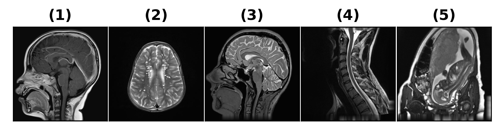
Figure 1: Test Images

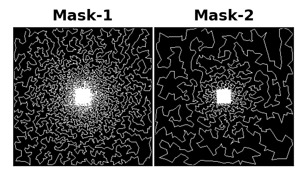
Figure 2: Masks for sampling trajectories

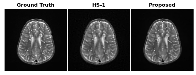
Figure 3: Result for Im2 and Mask 2

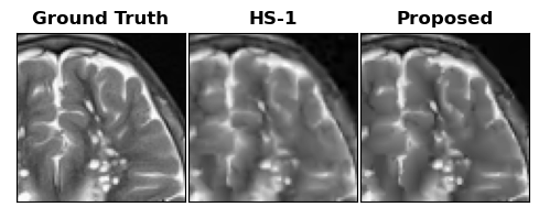
Figure 4: Zoomed view of the result

5 Theoretical Results and Proofs

5.1 Properties of QSHS penalty

Now, we formally define the concept of restricted proximal regularity.

Definition 5.1.

(Restricted proximal regularity) A lower semi-continuous function $f:\mathbb{R}^{n}\rightarrow\mathbb{R}\cup\{\infty\}$ is restricted proximal regular if for any $M>0$ and any bounded set $\Omega$ there exists $\gamma\equiv\gamma(M,\Omega)$ such that the following holds for all $y\in\Omega,x\in\{\,x\in\Omega\mid\|p\|\leq M\ \ \ \forall p\ \ \ \in\partial f(x)\,\}$, and for all $d\in\partial f(x)$:

$$f(y)-f(x)-\langle d,(y-x)\rangle\geq-\frac{\gamma}{2}\|y-x\|^{2}.$$

The following proposition establishes the restricted proximal regularity of the proposed QSHS penalty. The proof proceeds by following the methodology outlined in the proof of restricted proximal regularity for $l_{q}$ norms ($q\in(0,1)$) as presented in [13]. However, a notable challenge in this context is the lack of a closed-form expression for the penalty. Consequently, we use the abstract properties of $g_{q}$ to prove the result. propositionrpr Consider any $\mathbf{H}\in\mathbb{R}^{2\times 2},$ then $r(\mathbf{H})\stackrel{{\scriptstyle def}}{{=}}g_{q}(\sigma_{1}(\mathbf{H}))+g_{q}(\sigma_{2}(\mathbf{H}))$ is restricted proximal regular.

Proof.

We use the following result [25] for the sub-gradient: Let $H\in\mathbb{R}^{2\times 2}$ and $H=[U\ U_{1}]\begin{bmatrix}S&\mathbf{0}\\ \mathbf{0}&\mathbf{0}\\ \end{bmatrix}[V\ V_{1}]^{T}$ be the singular value decomposition (SVD) of $H$, $r(H)=\sum_{i=1}^{2}g_{q}(S_{ii}(\mathbf{H})),$ then $UDV^{T}+U_{1}\Theta V_{1}^{T}\in\partial r(H),$ where $D$ is diagonal matrix with entries $(D)_{ii}=g_{q}^{\prime}(S_{ii}),\text{ and }\Theta$ is any arbitrary matrix.

Without loss of generality we choose, $\Omega=\{\,X\in\mathbb{R}^{2\times 2}\mid\|X\|\leq P\,\}$. Now, for any $M,P>0$, we intend to show that

$$r(B)-r(A)-\langle T,B-A\rangle\geq-\frac{\gamma}{2}\|B-A\|^{2}$$

for all $B\in\Omega,A\in\Omega_{M}\stackrel{{\scriptstyle def}}{{=}}\{\,X\in\Omega\mid\|T\|\leq M,\ \ \ \forall T\ \ \ \in\partial r(X)\,\}$, and for all $T\in\partial r(A)$ . We do this in the following cases:

Case 1:

$\|B-A\|\geq\epsilon_{0}=\frac{1}{3}(g_{q}^{\prime})^{-1}(M)$ Note that the above condition is equivalent to

$$\frac{-\|B-A\|}{\epsilon_{0}}\leq-1.$$ (11)

First, it can be observed that,

$$r(B)-r(A)-\langle T,B-A \rangle\stackrel{{\scriptstyle a}}{{\geq}}-r(A)+\|T\|\|B-A\|,$$ (12)

$$\stackrel{{\scriptstyle b}}{{\geq}}-R_{max}-M\|B-A\|.$$ (13)

Here, $(a)$ is true as $r(\cdot)$ is non-negative and by Cauchy-Scwartz inequality; while $(b)$ is true as $T$ is bounded and $r(\cdot)$ is a continuous function on a bounded and closed set, therefore, it attains maximum $R_{max}.$ Now, using eq. 11 we obtain

$$r(B)-r(A)-\langle T,B-A\rangle{\geq}-\big{(}\frac{R_{max}+M\epsilon_{0}}{\epsilon_{0}^{2}}\big{)}\|B-A\|^{2}.$$ (14)

Case 2:

$\|B-A\|<\epsilon_{0}$. To prove this, we first define $\Omega^{\prime}=\{\,T\in\mathbb{R}^{n\times n}\mid\|T\|\leq P,\ \min_{i}\sigma_{i}(T)\geq\epsilon_{0}\,\}$.

Now, we decompose $B=U_{B}\Sigma_{B}V_{B}^{T}$, $B=U_{B}\Sigma_{B}^{(1)}V_{B}^{T}+U_{B}\Sigma_{B}^{(2)}V_{B}^{T}=B_{1}+B_{2},$ where all singular values of $B_{1}$ are greater than $\epsilon_{0}.$ Clearly, $B_{1}\in\Omega^{\prime}.$ We show that $A\in\Omega^{\prime}.$ This is proved by contradiction. Assume the contrary that $A\notin\Omega^{\prime}.$ This means, $\exists\ i$ such that $\sigma_{i}(A)<\epsilon_{0}\implies\sigma_{i}(A)<3\epsilon_{0}.$ Now, since $g_{q}^{\prime}(\cdot)$ is non-increasing, we have $g_{q}^{\prime}(\sigma_{i}(A))>g_{q}^{\prime}(3\epsilon_{0})=g_{q}^{\prime}((g_{q}^{\prime})^{-1}(M))=M.$ Let $A=U_{A}S_{A}V_{A}^{T}$ be the singular value decomposition of A. Define $T_{1}\stackrel{{\scriptstyle def}}{{=}}U_{A}S^{\prime}V_{A}^{T},$ where $\{S^{\prime}\}_{kk}=g_{q}^{\prime}(\{S_{A}\}_{kk})$ for all $k$. Now, by lemma $T_{1}\in\partial r(A).$ But, $\|T_{1}\|\geq\|S^{\prime}\|\geq g_{q}^{\prime}(\sigma_{i}(A))>M.$ This contradicts the fact that $A\in\Omega_{M}.$ Hence, $A\in\Omega^{\prime}.$ Now, we define a function, $F:\mathbb{R}^{n\times n}\rightarrow\mathbb{R}^{n\times n}$, which is defined as

$$F:X\mapsto U_{X}D_{X}^{\prime}V_{X}^{T}.$$

Here, $X=U_{X}D_{X}V_{X}^{T}$ is the singular value decomposition of $X$ and $D_{X}^{\prime}$ is a diagonal matrix which is defined as $(D_{X}^{\prime})_{ii}=g_{q}^{\prime}((D_{X})_{ii})$. Since $F$ is continuous on compact set on $\Omega^{\prime}$, it is Lipschitz continuous on $\Omega^{\prime}$ [26], this means $\|F(B)-F(A)\|\leq L\|B-A\|$. Now, by Taylor’s expansion we have:

$$r(B_{1})-r(A)-\langle B_{1}-A,U_{A}S^{\prime}V_{A}^{T}\rangle\geq\frac{-L}{2}\|B_{1}-A\|^{2}$$ (15)

. Now, $\|U_{2}^{T}U_{B}\|\leq\frac{\|A-B_{1}\|}{\epsilon_{0}}$ and $\|V_{2}^{T}V_{B}\|\leq\frac{\|A-B_{1}\|}{\epsilon_{0}}$ [27]. Now,

$$\langle U_{2}^{T}\Theta V_{2},B_{1}-A\rangle=\langle\Theta,U_{2}U_{B}^{T}\Sigma_{B}^{(1)}V_{B}V_{2}^{T}\rangle\geq-\frac{M^{2}\|B_{1}-A|\|^{2}}{\epsilon_{0}^{2}}.$$ (16)

Also, $r(B_{2})-<T,B_{2}>\geq 0$ and by triangle inequality we get:$\|B_{1}-A\|\leq\|B_{1}-B\|+\|B-A\|\leq 2\|B-A\|.$ Adding eq. 15 and eq. 16 we get,

$$r(B)-r(A)-\langle B-A,T\rangle\geq-(\frac{L}{2}+\frac{4M^{2}}{\epsilon_{0}^{2}})\|B-A\|^{2}.$$ (17)

∎

5.2 Properties of Restoration cost

The following helps us to establish that the restoration cost is coercive.

Claim 0.1.

If $\mathcal{N}(\mathcal{T})\cap\mathcal{N}(\mathcal{H})=\{\mathbf{0}\}$ the function $\|\mathcal{T}\mathbf{u}\|+\|\mathcal{H}\mathbf{u}\|_{*}\geq\gamma\|\mathbf{u}\|,\text{where }\gamma>0.$ Here, $\|\mathcal{H}\mathbf{u}\|_{*}$ is $\mathcal{H}S_{1}(\mathbf{u}),$ the conventional $l-1$ Hessian Schatten norm.

Proof.

The above statement is trivial if $\mathbf{u}=\mathbf{0}.$ If $\mathbf{u}\neq\mathbf{0}$, let $\hat{\mathbf{u}}=\frac{\mathbf{u}}{\|\mathbf{u}\|}$, then $\|\mathcal{T}\hat{\mathbf{u}}\|+\|\mathcal{H}\hat{\mathbf{u}}\|_{*}\geq\inf_{\|p\|=1}\|\mathcal{T}{\mathbf{p}}\|+\|\mathcal{H}{\mathbf{p}}\|_{*}$. Since, $\|\mathbf{p}\|=1$ is a compact set, $\exists\mathbf{p}_{min}$ (with $\|\mathbf{p}_{min}\|=1$) such that $\inf_{\|p\|=1}\|\mathcal{T}{\mathbf{p}}\|+\|\mathcal{H}{\mathbf{p}}\|_{*}=\|\mathcal{T}{\mathbf{p}_{min}}\|+\|\mathcal{H}{\mathbf{p}_{min}}\|_{*}$. Define, $\gamma=\|\mathcal{T}{\mathbf{p}_{min}}\|+\|\mathcal{H}{\mathbf{p}_{min}}\|_{*}.$ Clearly, $\gamma\neq 0$ as we will get a vector in intersection of the null spaces, i.e. $\mathbf{p}_{min}\in\mathcal{N}(\mathcal{T})\cap\mathcal{N}(\mathcal{H})$, this contradicts the hypothesis. Re-substituting $\hat{\mathbf{u}}=\frac{\mathbf{u}}{\|\mathbf{u}\|}$ completes the proof. ∎

*

Proof.

Without loss of generality, we prove the theorem for $\rho=1.$ Consider the level set $\mathcal{L}_{\eta}(f)\stackrel{{\scriptstyle def}}{{=}}\{\,\mathbf{x}\mid f(\mathbf{x})\leq\eta\,\}.$ Now, if $f(\mathbf{x})\leq\eta\implies\frac{1}{2}\|\mathcal{T}\mathbf{x}-\mathbf{m}\|^{2}\leq\eta.$ Now, by triangle inequality

$$\|\mathcal{T}\mathbf{x}\|\leq\sqrt{2\eta}+\|\mathbf{m}\|.$$ (18)

Since, $\mathbf{u}\in\mathcal{L}_{\eta}(f)\implies g_{q}(\sigma_{i}([\mathcal{H}\mathbf{u}]_{\mathbf{r}}))\leq\eta\ \ \ \forall\mathbf{r}\text{ and }i=1,2.$ As $g_{q}(\cdot)$ is coercive for $q\in(0,1)$, we have $\sigma_{i}([\mathcal{H}\mathbf{u}]_{\mathbf{r}})\leq M$ for some $M>0.$ This above statement is true because of the fact that any level set of a coercive function is compact. By Taylor’s series of $g_{q}$ around $0$ we can see that: $g_{q}(\sigma_{i}([\mathcal{H}\mathbf{u}]_{\mathbf{r}}))=g_{q}^{\prime}(\gamma_{i,\mathbf{r}})\sigma_{i}([\mathcal{H}\mathbf{u}]_{\mathbf{r}})$ for $\gamma_{i,\mathbf{r}}\in[0,2M)$. Since, $g_{q}^{\prime}(\cdot)$ is decreasing, therefore, $g_{q}^{\prime}(\gamma_{i,\mathbf{r}})\geq g_{q}^{\prime}(2M)\stackrel{{\scriptstyle def}}{{=}}C_{2M}.$ Hence, $\mathbf{x}\in\mathcal{L}_{\eta}(f)\implies C_{2M}\|\mathcal{H}\mathbf{u}\|_{*}\leq\sum_{\mathbf{r}}g_{q}(\sigma_{1}([\mathcal{H}\mathbf{u}]_{\mathbf{r}}))+g_{q}(\sigma_{2}([\mathcal{H}\mathbf{u}]_{\mathbf{r}})\leq\eta.$ Now, we use the following 0.1 to show that the level set $\mathcal{L}_{\eta}(f)$ is bounded. Using, 0.1 we get

$$\gamma\|\mathbf{u}\|\leq\|\mathcal{T}\mathbf{u}\|+\|\mathcal{H}\mathbf{u}\|_{*}\leq\frac{\eta}{C_{2M}}+\sqrt{2\eta}+\|\mathbf{m}\|.$$ (19)

This means the level set $\mathcal{L}_{\eta}(f)$ is bounded. Combining with the fact the level set is closed as $f(\cdot)$ is continuous implies that the level set is compact. As this is true for any level set, therefore $f$ is coercive.∎

5.3 Proof of convergence

$N_{iter}\leftarrow 1000$;

$\mathbf{u}^{(0)}=\mathbf{0}$;

$\mathbf{v}^{(0)}=\mathbf{0}$;

$\mathbf{w}^{(0)}=\mathbf{0}$;

if $i\leq N_{iter}$ then

       $\mathbf{u}^{(i+1)}\leftarrow\operatorname*{arg\,min}_{\mathbf{u}}\mathcal{L}_{\beta}(\mathbf{u},\mathbf{v}^{(i)},\mathbf{w}^{(i)})$;

       $\mathbf{v}^{(i+1)}\leftarrow\operatorname*{arg\,min}_{\mathbf{v}}\mathcal{L}_{\beta}(\mathbf{u}^{(i+1)},\mathbf{v},\mathbf{w}^{(i)})$;

       $\mathbf{w}^{(i+1)}\leftarrow\mathbf{w}^{(i)}+\beta(\mathbf{A}\mathbf{u}^{(i+1)}+\mathbf{B}\mathbf{v}^{(i+1)})$;

       $i\leftarrow i+1$;

      

Algorithm 1 Non-convex ADMM

We will use the following theorem by [13] to show the convergencve of our algorithm.

Literature Theorem 5.1.

([13], theorem 2.2) Consider the minimization of the function $\phi(\mathbf{u},\mathbf{v})=h(\mathbf{v})+g(\mathbf{v})$ subject to $\mathbf{A}\mathbf{u}+\mathbf{B}\mathbf{v}=\mathbf{0}$ by non-convex ADMM algorithm (Algorithm 1). Define the augmented Lagrangian, $\mathcal{L}_{\beta}(\mathbf{u},\mathbf{v},\mathbf{w})\stackrel{{\scriptstyle def}}{{=}}\phi(\mathbf{u},\mathbf{v})+\mathbf{w}^{T}(\mathbf{A}\mathbf{u}+\mathbf{B}\mathbf{v})+\frac{\beta}{2}\|\mathbf{A}\mathbf{u}+\mathbf{B}\mathbf{v}\|^{2}.$ If

C1

: $\phi(\mathbf{u},\mathbf{v})$ is coercive on the set $\{\,(\mathbf{u},\mathbf{v})\mid\mathbf{A}\mathbf{u}+\mathbf{B}\mathbf{v}=\mathbf{0}\,\};$

C2

: $Im(A)\subset Im(B)$, where $Im$ denotes the image of the linear operator;

C3

:$\mathbf{A}$ and $\mathbf{B}$ are full column rank;

C4

: $g$ is restricted proximal regular, and

C5

:$h$ is Lipschitz smooth,

then algorithm generates a bounded sequence that has atleast one limit point, and each limit point is a stationary point of $\mathcal{L}_{\beta}(\cdot)$

Now, we show the convergence of algorithm using the above theorem.

*

Proof.

We establish the validity of the aforementioned theorem by fulfilling the conditions ((C1)-(C5)) of 5.1. In comparison to the splitting presented in section 3, we set $h\equiv\frac{1}{2}\|\mathcal{T}(\cdot)-\mathbf{m}\|_{2}^{2}$ and $g\equiv\rho\sum_{\mathbf{r}}f(\cdot)+I_{S}(\cdot)$. The operator $\mathbf{A}$ is analogous to a linear operator, satisfying $\mathcal{A}(\mathbf{u})-\mathbf{v}=\mathbf{0}$. For each pixel location $\mathbf{r}$, $\mathcal{A}:[\mathbf{u}]_{\mathbf{r}}\rightarrow([\mathcal{H}\mathbf{u}]_{\mathbf{r}},[\mathbf{u}]_{\mathbf{r}})$. Regarding the constraints, it is evident that $\mathbf{B}$ corresponds to the negative identity matrix.

(C1) follows from section 3, and (C4) follows from definition 5.1. (C2) is trivial since $\mathbf{B}$ is the negative identity. (C5) holds true due to the quadratic nature of the data-fitting cost. To ascertain (C3), we must demonstrate that $\mathcal{N}(\mathbf{B})=\mathbf{0}$ and $\mathcal{N}(\mathbf{A})=\mathbf{0}$. Since $\mathbf{B}$ is the negative identity matrix, $\mathcal{N}(\mathbf{B})=\mathbf{0}$. For $\mathbf{A}$, let $\mathcal{A}(\mathbf{z})=\mathbf{0}$, implying $[\mathcal{H}\mathbf{z}]_{\mathbf{r}}=\mathbf{0}$ and $[\mathbf{z}]_{\mathbf{r}}=\mathbf{0}$ for all $\mathbf{r}$, which concludes $\mathbf{z}=\mathbf{0}$. Hence, all the conditions are met. The next step is to establish that the stationary point of the augmented Lagrangian coincides with that of the restoration cost. Suppose $(\mathbf{u}^{*},\mathbf{v}^{*},\mathbf{w}^{*})$ is the stationary point of the augmented Lagrangian; this implies:

1. $\mathcal{A}\mathbf{u}^{*}-\mathbf{v}^{*}=\mathbf{0}$,

2. $\nabla h(\mathbf{u}^{*})+\mathcal{A}^{T}\mathbf{w}^{*}=0,$ and

3. $\partial g(\mathbf{v}^{*})-\mathbf{w}^{*}\ni\mathbf{0}.$

Rearranging 2 and 3 we obtain $\nabla h(\mathbf{u}^{*})\in-\mathcal{A}^{T}\partial g(\mathbf{v}^{*})$. Now, we use 1 to get

$$-\nabla h(\mathbf{u}^{*})-\mathcal{A}^{T}\partial(\mathcal{A}\mathbf{u}^{*})\ni\mathbf{0}$$ (20)

$$\implies-\partial f(\mathbf{u}^{*})\ni\mathbf{0}$$ (21)

$$\implies\partial f(\mathbf{u}^{*})\ni\mathbf{0}.$$ (22)

∎

6 References

References

- [1] Scherzer O 1998 Computing 60 1–27 ISSN 0010-485X
- [2] Bredies K, Kunisch K and Pock T 2010 SIAM Journal on Imaging Sciences 3 492–526
- [3] Lysaker M, Lundervold A and Tai X C 2003 IEEE Transactions on image processing 12 1579–1590
- [4] Lefkimmiatis S, Ward J P and Unser M 2013 IEEE transactions on image processing 22 1873–1888
- [5] Lefkimmiatis S and Unser M 2013 IEEE transactions on image processing 22 4314–4327
- [6] Liu L, Li X, Xiang K, Wang J and Tan S 2017 IEEE transactions on medical imaging 36 2588–2599
- [7] Wang Q, Qu G and Ji D 2021 Mathematical Methods in the Applied Sciences 44 1674–1687
- [8] Arigovindan M, Fung J C, Elnatan D, Mennella V, Chan Y H M, Pollard M, Branlund E, Sedat J W and Agard D A 2013 Proceedings of the National Academy of Sciences 110 17344–17349
- [9] Nikolova M, Ng M K and Tam C P 2010 IEEE Transactions on Image Processing 19 3073–3088
- [10] Nikolova M 2005 Multiscale Modeling & Simulation 4 960–991
- [11] Sidky E Y, Chartrand R and Pan X 2007 Image reconstruction from few views by non-convex optimization 2007 IEEE Nuclear Science Symposium Conference Record vol 5 pp 3526–3530
- [12] Woodworth J and Chartrand R 2016 Inverse Problems 32 075004
- [13] Wang Y, Yin W and Zeng J 2019 Journal of Scientific Computing 78 29–63
- [14] Glowinski R and Marroco A 1975 Revue française d’automatique, informatique, recherche opérationnelle. Analyse numérique 9 41–76
- [15] Gabay D and Mercier B 1976 Computers & mathematics with applications 2 17–40
- [16] Davis D and Yin W 2016 Convergence rate analysis of several splitting schemes Splitting methods in communication, imaging, science, and engineering (Springer) pp 115–163
- [17] Chartrand R and Wohlberg B 2013 A nonconvex admm algorithm for group sparsity with sparse groups 2013 IEEE international conference on acoustics, speech and signal processing (IEEE) pp 6009–6013
- [18] Liavas A P and Sidiropoulos N D 2015 IEEE Transactions on Signal Processing 63 5450–5463
- [19] Wen Z, Yang C, Liu X and Marchesini S 2012 Inverse Problems 28 115010
- [20] Li G and Pong T K 2015 SIAM Journal on Optimization 25 2434–2460
- [21] Hong M, Luo Z Q and Razaviyayn M 2016 SIAM Journal on Optimization 26 337–364
- [22] Magnússon S, Weeraddana P C, Rabbat M G and Fischione C 2015 IEEE Transactions on Control of Network Systems 3 296–309
- [23] Wang F, Cao W and Xu Z 2018 Science China Information Sciences 61 1–12
- [24] Rudin L I, Osher S and Fatemi E 1992 Physica D: nonlinear phenomena 60 259–268
- [25] Watson G A 1992 Linear Algebra Appl 170 33–45
- [26] Ding C, Sun D, Sun J and Toh K C 2018 Mathematical Programming 168 509–531
- [27] Li R C and Stewart G 2000 Linear Algebra and its Applications 313 41–51