Composite scalar bosons masses: Effective potential versus Bethe-Salpeter approach

Abstract

Ten years ago the $125$ GeV Higgs resonance was discovered at the LHC [1, 2] , if this boson is a fundamental particle or a particle composed of new strongly interacting particles is still an open question. If this is a composite boson there are still no signals of other possible composite states of this scheme, a possible solution to this problem was recently discussed in Refs.[30, 31], where it is argued that the Higgs boson can be a composite dilaton [30]. In this work, considering an effective potential for composite operators we verify that the potential responsible for a light composite scalar boson of $O(120)GeV$, behaves like $\propto\Phi^{4}$ suggesting that if the Higgs boson is a composite scalar it may be a composite dilaton.

I Introduction

The Higgs boson discovery was one of the major particle physics breakthrough in the last decades. If this boson is composed by new strongly interacting particles is still an open question , composite scalar bosons appear in the context of Technicolor theories (TC) [3, 4, 5], which usually have a composition scale of order of $\Lambda_{C}\geq 1$TeV. Another possibility raised a few years ago is to have a Higgs arising as a composite pseudo-Goldstone boson (PGB) from the strongly interacting sector. In this case the Higgs mass is protected by an approximate global symmetry and is only generated via quantum effects, models based on this approach are usually called composite Higgs models[29].

Technicolor, was inspired in QCD, to provide a natural and consistent quantum-field theoretic description of electroweak (EW) symmetry breaking, without elementary scalar fields. Crafting a realistic Technicolor model can be a very precise engineering problem.

Over the years different models have emerged considering different approaches to obtain large mass anomalous dimension ($\gamma$), which in summary, can be classified as
(i) Quasi-conformal TC theories[6, 7, 8, 9, 10, 11], where $\gamma(N_{TC},n_{F})$, and it is possible to obtain an almost conformal behavior when the fermions are in the fundamental representation, $R=F$ , introducing a large number of TC fermions $n_{F}$. Nonetheless, the cost of such procedure may be a large S parameter, in an the similar way an almost conformal TC theory can also be obtained when the fermions are in larger representations that the fundamental one[12, 13, 14, 15].
(ii) Methods of lattice gauge theory, as the authors in Refs.[16, 17, 18, 19] has demonstrated, the conformal window for the $SU(3)$ gauge theory lies in the range $8<n_{f}<12$, and in this region is possible indeed have a slowly running coupling (or $\beta\approx 0$ ).
(iii) Gauged Nambu-Jona-Lasinio models, in this case the existence of an “effective” four-fermion interaction in TC dynamics[20, 21, 22, 23, 24, 25, 26], could also be responsible by large $\gamma$ values.

As proposed by Holdom[27], a light composite scalar boson may be generated when the strong interaction theory (or TC) has a large mass anomalous dimension ($\gamma$), the discussion of how these scenarios might lead to a light composite scalar boson is presented in Refs.[28]. Assuming these different scenarios, calculations involving effective Higgs Lagrangians led to different predictions regarding the masses of composite scalar bosons.

The self-energy of the new fermions (technifermions) responsible for the composite states, that are characterized by a large mass anomalous dimension $\gamma$, result in mass diagrams whose calculation do not scale with the naive dimensions. In this case, the self-energy $\Sigma_{\textnormal{\tiny}\textsc{F}}(p^{2})$ at large momenta is proportional to

$$\Sigma_{\textnormal{\tiny}\textsc{F}}(p^{2})\propto\frac{\mu_{\textnormal{\tiny}\textsc{F}}^{3}}{p^{2}}(p^{2}/\mu_{\textnormal{\tiny}\textsc{F}}^{2})^{\gamma/2}.$$ (1)

where $\mu_{\textnormal{\tiny}\textsc{F}}\sim O(1)TeV$ is the typical composition or dynamical fermion mass scale.

The absence of signals of a large scalar boson sector in the experimental data, as well as a possible explanation of a light Higgs boson, has been beautifully discussed recently in Refs.[30, 31]. In that references it is argued that the Higgs boson, a Gildener-Weinberg dilaton [32], could be a composite dilaton [30].

Recently, considering constituents of same mass, we computed the composite scalar mass using Bethe-Salpeter equations (BSE) [33]. The calculation was performed with the help of an ansatz in the form of Eq.(1) for the constituent self-energy dependent on the mass anomalous dimension, the results obtained indicate how the scalar mass $M_{S}$ can vary with the mass anomalous dimension($\gamma$) leading to $M_{S}(\gamma)=A(\gamma)\mu_{\textnormal{\tiny}\textsc{F}}$. At this point, we must emphasize that there are not in the literature other calculations using the Bethe-Salpeter equations to address the question of a possible composite Higgs boson in Technicolor models. Usually, the solutions of the Bethe-Salpeter equations are used in hadronic physics, as, for example, in the study of meson spectroscopy[34].

In this work, considering effective potential for composite operators[35, 36, 37] we extend the discussion started in Ref.[33], in particular we verify that the potential responsible for a light composite scalar boson, $M_{S}\sim O(120)GeV$, behaves like $\propto\Phi^{4}$, indicating the possibility that the Higgs boson may in principle be a composite dilaton as suggested in Refs.[30, 31], and its mass can be smaller than the composition scale as long as we have large anomalous dimensions. Moreover, we determine the mass obtained for the lightest pseudo scalar boson, $\Pi^{0}\sim\bar{N}N$ and we retrieve the result described in Ref.[38], assuming the Bethe-Salpeter equations.

This paper is organized as follows: In section II we determine the effective potential for composite operators for the constituent self-energy considered in Ref.[33], in the section III we calculate the scalar composite scalar mass from the effective potential. With the help of Bethe-Salpeter equations (BSE), assuming the same conditions employed in the previous section, in the section IV we calculate the scalar boson mass and compare with the previous result. At the end of this section, we determine $\Pi^{0}$ mass from the BSE equations. The section V contains our conclusions.

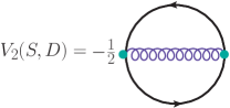
Figure 1: Two-particle irreducible contribution to the vacuum energy.

II The effective potential and the self-energy ansatz

II.1 The effective potential for composite operators

The effective potential for composite operators was proposed many years ago in Ref[35] by Cornwall, Jackiw and Tomboulis, as complementary references we suggest to the reader [37, 39], where it is possible to find a detailed calculation of the composite scalar masses considering this method. The effective action for composite operators $\overline{\Gamma}(G)$ is a function of the Green functions denoted by $G=G_{n}$, and is stationary with respect to variations of $G_{n}$. The effective potential $V(G)$ is defined by the following equation

$$V(G_{n})\int d^{4}x=-\overline{\Gamma}(G)|_{ti},$$ (2)

where $(ti:=translation\,\,invariant)$ , and $V(G)$ can be written in terms of the complete fermion (S) and gauge boson (D) propagators, in the form

$$\!\!\!\!\!V(S,D)=-iTr\left(\ln S_{0}^{-1}S-S_{0}^{-1}S+1\right)+iV_{2}(S,D),$$ (3)

where in this expression the complete fermion propagator is represented by

$$S^{-1}(p)={\not{p}}A(p^{2})-B(p^{2})\,.$$ (4)

whereas, the free propagator is $S_{0}=i/{\not\!p}$, and we shall assume $A(q^{2})=1$ and $B(p^{2})=\Sigma(p^{2})$. In these equations, we are not considering contributions to the potential due to gauge and ghosts loops, we just are interested only in the fermionic bilinear condensation in the scalar channel, and will consider a non-abelian gauge theory, stronger than QCD, whose fermions form the composite scalar boson. In this case, we can consider the approximation where $D=D_{0}$ stands for the bare gauge boson propagator, that in Landau gauge, can be written as

$$g^{\mu\nu}D_{\mu\nu}(p-k)=\frac{3}{(p-k)^{2}}=3G(p-k).$$ (5)

In order to keep the above equations in a compact form, we are not writing the Lorentz and $SU(n)_{TC}$ indexes, as well as momentum integrals. The last term in Eq.(3), $V_{2}(S,D)$, corresponds to the sum of all two-particle irreducible vacuum diagrams, shown in Fig.(1), that can be analytically represented by

$$iV_{2}(S,D)=-\frac{i}{2}\,Tr(\Gamma S\Gamma SD),$$ (6)

where $\Gamma$ is the fermion proper vertex. An important property in the potential Eq.(3) is that its minimization with respect to the complete propagators ($S$ or $D$) , $\delta V/\delta(S,D)=0$, reproduce exactly the Schwinger-Dyson equations for the complete $S$ and $D$ propagators.

To obtain an effective Lagrangian for the composite scalar boson, it is better to compute the vacuum energy density which is given by the effective potential calculated at minimum subtracted by its perturbative part, which does not contribute to dynamical mass generation

$$\Omega_{V}=V(S,D)-V(S_{0},D_{0}),$$ (7)

After replacing the Eqs.(3), (4) and (5) in Eq.(7), now indicating the momenta integrals we can write

$$\Omega_{V}=i\int\frac{d^{4}p}{(2\pi)^{4}}Tr\left[\ln\left(1-\frac{\Sigma^{2}(p^{2})}{p^{2}}\right)+\frac{\Sigma^{2}(p^{2})}{p^{2}-\Sigma^{2}(p^{2})}\right.$$

$$\hskip 17.07182pt\left.+\frac{3C_{2}g^{2}(p^{2})\Sigma^{2}(p^{2})}{p^{2}(p^{2}-\Sigma^{2}(p^{2}))}i\int^{p^{2}}\frac{d^{4}k}{(2\pi)^{4}}\frac{\Sigma^{2}(k^{2})}{k^{2}(k^{2}-\Sigma^{2}(k^{2}))}\right],$$

(8)

where to obtain the above equation we assumed the angle approximation

$$\frac{g^{2}(p,k)}{(p-k)^{2}}=\frac{g^{2}(p^{2})}{p^{2}}\Theta(p^{2}-k^{2})+\frac{g^{2}(k^{2})}{k^{2}}\Theta(k^{2}-p^{2})$$

and $\Theta$ is the Heaviside step function. In the Euclidean space we can write $\Omega_{V}$ as

$$\Omega_{V}=\Omega_{V_{A}}+\Omega_{V_{B}}$$ (9)

where

$$\Omega_{V_{A}}=-\frac{N_{TC}n_{F}}{8\pi^{2}}\int p^{2}dp^{2}\left[\ln\left(1+\frac{\Sigma^{2}(p^{2})}{p^{2}}\right)-\frac{\Sigma^{2}(p^{2})}{p^{2}+\Sigma^{2}(p^{2})}\right],$$ (10)

and

$$\Omega_{V_{B}}=+\frac{N_{TC}n_{F}}{8\pi^{2}}\int p^{2}dp^{2}\left[\frac{3C_{2}\alpha_{TC}(p^{2})\Sigma^{2}(p^{2})}{2\pi p^{2}(p^{2}+\Sigma^{2}(p^{2}))}\int^{p^{2}}\frac{dk^{2}\Sigma^{2}(k^{2})}{k^{2}(k^{2}+\Sigma^{2}(k^{2}))}\right],$$ (11)

in these equations, $N_{TC}$ is the number of technicolors (techniquarks are in the fundamental representation $R=F$ of $SU(N_{TC})$), and $n_{F}=n_{F}(R)$ is the number of technifermions(F).

II.2 The self-energy ansatz

In usual calculations involving the Schwinger-Dyson equations, the self-energy $\Sigma(p^{2})$ is obtained from the numerical solutions for the fermionic propagators. In this work we will assume the ansatz employed in [33], that is a function of the mass anomalous dimension $\gamma$, and has the form

$$\Sigma(p^{2})=\frac{\mu^{3}}{p^{2}+\mu^{2}}\left(\frac{p^{2}+\mu^{2}}{\mu^{2}}\right)^{\kappa}\,$$ (12)

where $\kappa=\gamma/2$. In this expression $\mu=\mu_{F}$ is the dynamically generated mass, and Eq.(12) behaves in the infrared region as $\mu$ , as $\kappa\rightarrow 0$, Eq.(12) leads to self-energy roughly equal to $\mu^{3}/p^{2}$ in the asymptotic region , which is the behavior predicted by a standard operator product expansion (OPE) for the techniquark self-energy $\Sigma(p^{2})$ for $\langle\bar{Q}Q\rangle\sim\mu^{3}$.

However , when $\kappa\rightarrow 1$(or $\gamma\to 2)$ Eq.(12) can be written in the form

$$\Sigma(p^{2})\approx\mu\left[1+\delta_{1}\ln\left[(p^{2}+\mu^{2})/\mu^{2}\right]\right]^{-\delta_{2}}\,,$$ (13)

where to arrive at this form, $\delta_{1}$ and $\delta_{2}$ are obtained from $\gamma$ when expanded as a function of the running coupling $g^{2}(p^{2})$. In this case, the self-energy stands for an extreme walking gauge theory, and the standard OPE prediction is modified by a large anomalous dimension $(\gamma)$, and the self-energy behaves as $\mu\ln^{-\gamma}(p^{2}/\mu^{2})$ asymptotically, mapping the SDE possible solutions in the full Euclidean space, allow us to obtain an equation for the scalar mass $M_{S}$ as a function of $\gamma$.

III The effective Lagrangian for composite scalar bosons

III.1 The kinetic term of the effective action

In this section, we shall consider the problem of generating one light composite scalar boson in the context of the effective potential assuming the self-energy ansatz given by Eq.(12). As pointed out recently in Ref.[30, 31] a composite Gildener-Weinberg dilaton should result from an effective potential that, at leading order(0), is proportional to

$$V(\Phi)_{0}\propto\Phi^{4},$$ (14)

where $\Phi$ is a composite effective field. A theory that generates a composite Higgs boson, where $\Phi\propto\bar{Q}Q$ and $\bar{Q}Q$ corresponds to a bound state of techniquarks Q, should naturally not contain a quadratic term in the effective potential.

The $\Sigma^{2}(p^{2})/p^{2}$ term in the logarithm in Eq.(10) can be expanded, the contribution of the $\Sigma^{2}$ term in this equation eventually cancels out, leading to the absence of quadratic terms in the effective potential. This cancellation is a consequence of the fact that $\Sigma(p^{2})$ obeys the linear homogeneous SDE for the fermion propagator[37, 39].

In order to obtain an expression for the effective Lagrangian of composite scalars bosons from Eq.(12), we will reconsider the approach described in Ref.[36] to determine a complete effective theory, including the kinetic term of the effective action. The fermionic propagator can be described by a fermion bilinear that has the following operator expansion

$$S(x,y)=\langle\Omega|T[\chi(x+\frac{1}{2}y)\psi(x-\frac{1}{2}y)]|\Omega\rangle\,\,\,{}^{\,\,\sim}_{y\rightarrow 0}\,\,\,C(y)\phi(x),$$ (15)

where in the above equation $C(y)$ is a $c$-number function, and $\phi(x)$ acts like a dynamical effective scalar field. Taking into account the structure of the real vacuum, where the propagator is a fermion bilinear and $\Sigma$ depending on two momenta $\Sigma(p,k)$, we can consider the Fourier transform of above equation and write

$$\Sigma(p,k)\sim\phi(k)\Sigma(p)\,.$$ (16)

In the effective action, $\phi(x)$ can be seen as a variational parameter whose minimum will be indicated by $\phi$, corresponding to the leading contribution of its expansion around $k=0$. A more detailed presentation of this approach can be seen in Ref.[36], as commented in Ref.[39], depending on the theory dynamics, i.e. $\kappa\in[0,1]$ in Eq.(12), when the self-energy decreases slowly with the momentum, which corresponds to the case when $\kappa\to 1$ in Eq.(12), the kinetic term is important for the characterization of the effective Lagrangian.

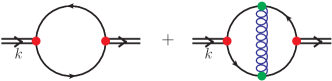
Figure 2: Diagrams contributing to the kinetic term in the effective Lagrangian.

The kinetic term is given by the polarization diagrams ($\Pi(k^{2},\phi)$) shown in Fig.(2), these diagrams are responsible in the effective Lagrangian for terms of the form

$$\Omega_{K}=\int d^{4}x\frac{1}{2}\partial_{\mu}\phi\partial^{\mu}\phi\,.$$ (17)

When the diagrams of Fig.(2) are calculated it is possible to verify that this term will be multiplied by a non-trivial function ($Z(\kappa)$) , which has a dependency with ($N_{TC}$), and the number of fermions ($n_{F}$), and also $\gamma$, once we consider the anzatz for $\Sigma$ described by Eq.(12). This non-trivial function, that must normalize the scalar composite field $\phi$, was obtained in the Ref.[36] and can be written as

$$(Z(\kappa))^{-1}\approx\frac{N_{TC}n_{F}}{4\pi^{2}}\int dp^{2}\frac{(p^{2})^{2}(\Sigma(p^{2})/\mu)^{2}}{(p^{2}+\mu^{2})^{3}}\,\,\,,$$ (18)

the index $\kappa=\frac{\gamma}{2}$ is the same one appearing in Eq.(12).

III.2 The effective Lagrangian

Once we have characterized the kinetic term in the effective Lagrangian, now we can calculate the expansion for $\Sigma(p^{2})/p^{2}<<1$ in Eq.(9), and write this equation in terms of the variational field $\phi$ in the form [37, 39]

$$\tilde{\Omega}\approx\int d^{4}x\left[\frac{1}{2Z^{(\kappa)}}\partial_{\mu}\phi\partial^{\mu}\phi-\lambda_{4(0)}\phi^{4}+\lambda_{6(0)}\phi^{6}-...\right],$$

(19)

where now

$$\lambda_{4(0)}=\,\,\frac{N_{TC}n_{F}}{8\pi^{2}}\,\int dz\left(\,\,\,-\frac{3}{4}\frac{f^{4}(z)}{z}-f^{2}(z)\frac{df^{2}(z)}{dz}\,\,\,+\right.$$

$$\left.+\frac{2}{3}\frac{f^{6}(z)}{z^{2}}+\frac{f^{4}(z)}{z^{2}}\frac{df^{2}(z)}{dz}-\frac{5}{8}\frac{f^{8}(z)}{z^{3}}-\frac{f^{6}(z)}{z^{2}}\frac{df^{2}(z)}{dz}+\right.$$

$$\left.+\frac{3}{5}\frac{f^{10}(z)}{z^{4}}+\frac{f^{8}(z)}{z^{3}}\frac{df^{2}(z)}{dz}...\right)$$

$$\lambda_{6(0)}=-\frac{\lambda_{4(0)}}{\mu^{2}},$$ (20)

with $z=\frac{p^{2}}{\mu^{2}}$ and $f(z)=\frac{\Sigma(p^{2})}{\mu}$. The effective coupling constants $\lambda_{4(0)}$ and $\lambda_{6(0)}$ are determined from Eqs.(9) and (12).

In Eq.(11) $C_{2}$ is the Casimir operator for fermions, and we consider $g^{2}(p^{2})=g^{2}$ and also the MAC hypothesis[40, 41] in this calculation, where $\frac{g^{2}C_{2}}{4\pi}\approx C_{2}\alpha\approx\frac{\pi}{3}$, that lead to

$$\lambda_{4(0)}(\kappa)\approx\frac{N_{TC}n_{F}}{8\pi^{2}}\left[\frac{1}{2}+\frac{3}{16\kappa-16}+\frac{2}{3(7-6\kappa)}\,+\right.$$

$$\hskip 85.35826pt\left.-\frac{5}{8(10-8\kappa)}+\frac{3}{5(13-10\kappa)}+\right.$$

$$\hskip 85.35826pt\left.-\frac{(\kappa-1)\left(68\kappa^{2}-172\kappa+109\right)}{(4\kappa-5)(6\kappa-7)(10\kappa-13)}\right]$$

$$\lambda_{6(0)}(\kappa)\approx-\frac{1}{\mu^{2}}\lambda_{4(0)}(\kappa).$$ (21)

The Eq.(19) differs from a conventional scalar field Lagrangian by the kinetic term $Z(\kappa)$, therefore, the final effective Lagrangian comes out when we normalize the scalar field $\Phi$ according to $\Phi\equiv[Z(\kappa)]^{-\frac{1}{2}}\phi$ , leading to the normalized effective Lagrangian $\tilde{\Omega}(\kappa)$

$$\tilde{\Omega}(\kappa)=\int d^{4}x\left[\frac{1}{2}\partial_{\mu}\Phi\partial^{\mu}\Phi-\tilde{\lambda}_{4}(\kappa)\Phi^{4}+\tilde{\lambda}_{6}(\kappa)\Phi^{6}-...\right],$$

(22)

where, assuming Eq.(12), the normalization function $Z(\kappa)$ can be determined to be equal to

$$Z(\kappa)\approx\frac{4\pi^{2}}{N_{TC}n_{F}}\left(2-2\kappa\right).$$ (23)

The coupling constants $\lambda_{4(0)}$, $\lambda_{6(0)}$ indicated in Eq.(21), were replaced by the respective normalized ones $\tilde{\lambda}_{4}(\kappa)\equiv Z^{2}(\kappa)\lambda_{4(0)}$ and $\tilde{\lambda}_{6}(\kappa)\equiv Z^{3}(\kappa)\lambda_{6(0)}$. Therefore, the scalar mass $M^{2}_{S}(\kappa)$ can be determined from the effective potential Eq.(22) at the minimum from

$$M^{2}_{S}(\kappa)=\frac{\partial^{2}\tilde{\Omega}(\kappa)}{\partial\Phi^{2}}{|}_{{}_{\Phi=\Phi_{min}}}\!\!\!\!\!\approx 2\frac{(\tilde{\lambda}_{4}(\kappa))^{2}}{\tilde{\lambda}_{6}(\kappa)}\approx 2Z(\kappa)\lambda_{4(0)}(\kappa)\mu^{2}.$$ (24)

Note that the effective potential depends on the TC fermionic representation $R$, the product $(N_{TC}\times n_{F}(R))$, and the anomalous dimension $\gamma=\gamma(N_{TC},n_{F}(R))$. In order to present numerical results as a function of $\gamma$ (which is also a function of $N_{TC}$ and $n_{F}(R)$), we will simply assume that TC is not so different from QCD and adopt $N_{TC}=3$ and $n_{F}=5$[33], expecting that we can still present the variation of the TC masses with $\gamma$ when determined from the effective potential. At this point we must point out that

$$M^{2}_{S}(\kappa)/\mu^{2}\approx 2Z(\kappa)\lambda_{4(0)}(\kappa)\propto\frac{\not{\!\!N}_{TC}\not{\!n}_{F}}{\not{\!\!N}_{TC}\not{\!n}_{F}}f(\kappa)\propto f(\kappa)$$

i.e. the dependence of $M^{2}_{S}(\gamma,N_{TC},n_{F}(R))=M^{2}_{S}(\gamma)$ results only from the anzatz dependency, Eq.(12), with $\gamma$.

In usual perturbative QCD, we can expect $\gamma\sim 0$, however, as we commented large mass anomalous dimensions $\gamma$ could be obtained in scenarios as listed (i)-(iii).

An increase of $n_{F}$, for example as the authors in Refs.[16, 17, 18, 19] have demonstrated the conformal window for the $SU(3)$ gauge theory lies in the range $8<n_{f}<12$, or the consideration of higher TF representations $R>F$[12, 13, 14, 15], would lead to large values to $\gamma$ needed to produce changes in the TC mass function. In calculations involving the Eq.(12), we will consider $\gamma$ as an adjustable parameter, and if the Higgs boson is a composite particle, a realistic TC model could probably be characterized by one of these possible scenarios.

IV The TC scalar mass: BSE versus effective potential approach

IV.1 The $SU(N)_{TC}$ scalar masses

In this section, we will reconsider the approach employed in Ref.[33] for the characterization of the TC scalar and pseudo scalar masses using the Bethe-Salpeter equations (BSE).

We will assume that (BSE) equations described in Refs.[42, 43, 44], with the approximations discussed in[33], with the difference that in this work we will consider $G_{\rho\nu}(k-q)$ given by Eq.(5), in order to compare the results obtained with the effective potential.

The Bethe-Salpeter equation can be written as

$$\chi^{tc}(p,q)=-\imath\int\frac{d^{4}k}{(2\pi)^{4}}S(q+\alpha p)K_{\rho\nu}(p,k,q)S(q-\beta p),$$

$$K_{\rho\nu}(p,k,q)=\gamma_{\rho}\chi^{tc}(p,k)\gamma_{\nu}G_{\rho\nu}(k-q),$$ (25)

where in the above expression $\chi^{tc}$ is the technicolor(tc) BS wave function, $\alpha$ and $\beta$ characterize the fraction of momentum carried by the constituents, with $\alpha+\beta=1$.

In the calculation, we will consider that each constituent carries half of the momentum , i.e. $\alpha=\beta=1/2$. In the Eq.(25) the fermion propagator is given by (4), and the BSE solution appear as an eigenvalue problem for $p^{2}=M^{2}$, where $M$ is the bound state mass.

In the equation(25) the variables are $p,q,k$, $k$ is integrated, and we remain with an equation in $q$ that will have a solution for $p^{2}=M^{2}$. To solve this integral equation, to scalar channel we can project $\chi^{tc}(p,q)=\chi^{tc}_{S}(p,q)$ into four coupled homogeneous integral equations given by

$$\chi^{tc}_{S}(p,q)=\chi_{S0}+\not{p}\chi_{S1}+\not{q}\chi_{S2}+[\not{p},\not{q}]\chi_{S3},$$ (26)

which are functions of $p^{2}$, $q^{2}$ and $p.q=pqcos\theta$. It is possible to expand $\chi^{tc}(p,q)$ in terms of Tschebyshev polynomials, and these equations can be truncated at a given order determined by the relative size of the next-order functions. A satisfactory solution can be obtained by keeping only some terms, like $\chi_{S(0,1)}^{(0)},\chi_{S(1)}^{(0,1)},\chi_{S(2)}^{(0,1)}$.

In addition to the above considerations we will consider constituents of same mass $m=m_{a}=m_{b}$, with $m=\Sigma(x+\frac{1}{4}p^{2})$, where $x=q^{2}/\mu^{2}$and $\mu=\mu_{tc}$ is the characteristic mass scale of the binding forces(TC).

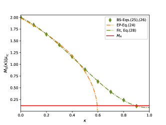
Figure 3: Scalar masses $M_{S}(\kappa)$ considering different approaches. The contextualization of the curves behavior are described in the text.

The procedure for determining $M_{S}(\kappa)$ is the same one described in Ref.[33]. In Fig.3 we present the behavior obtained for $M_{S}(\kappa)/\mu_{tc}$ considering the anzats for $\Sigma(p^{2})$ given by Eq.(12), assuming Eq.(24) and the corresponding result obtained from Eq.(25). As in Eq.(24) the scalar mass depicted in the Fig.3 is just a function of $\gamma$, which is an adjustable parameter.

In this figure we normalize ours results for $M_{S}$ in terms of

$$M_{S}=2\mu_{tc}.$$ (27)

associated to a negligible $\gamma$.

The choice of this normalization is based on the result described in Ref.[45], where Delbourgo and Scadron verified analytically with the help of the homogeneous BSE equations, that the sigma meson mass is given by $m_{\sigma}=2\mu_{dyn}$. We can use this result obtained for QCD to determine, by appropriate rescaling, the behavior of $M_{S}$ in TC models, where $\mu_{tc}=1TeV$.

In the Fig.3, the dot-dashed line in orange matches the results obtained from Eq.(24), the points denoted in ( $\blacklozenge$) represent the BSE numerical solutions obtained for $M_{S}(\kappa)/\mu_{tc}$. The line, in red, corresponds to the radius $M_{H}/\mu_{tc}$ for comparison with the $M_{S}(\kappa)/\mu_{tc}$ results.

In the dot-dashed line in olive we show the fit for $M_{S}(\kappa)/\mu_{tc}$ data with $R^{2}=0.99997$ which corresponds to

$$S(\kappa)=\frac{M_{S}(\kappa)}{\mu_{tc}}=2-1.3161\kappa-2.65806\kappa^{2}$$

$$\hskip 68.28644pt+1.38845\kappa^{3}+0.66806\kappa^{4}.$$ (28)

The expansion considered in Eq.(19) is not sensitive to the region of low momenta, which is captured by the BS equations, so that at $\gamma\approx 1$ the curves start to show a different behavior.

The comparison of the behavior exhibited for $M_{S}(\kappa)/\mu_{F}$, obtained with the different approaches, suggests that the potential responsible for generating the composite light scalar behaves like $\propto\Phi^{4}$, being characterized by $\gamma\sim O(1.2-1.8)$ indicating that the composite scalar boson $\Phi$ seems to behave like a dilaton as suggested in[30, 31].

IV.2 TC pseudo scalar masses

Let us suppose that the TC group is not so different from QCD where there are many pseudo Goldstone bosons (or technipions) resulting from the chiral symmetry breaking of the technicolor theory.

These technipions, besides the ones absorbed by the W’s and Z gauge bosons, can be classified for example according to[47]:

(a) Charged and neutral color singlets:

$$\Pi^{\pm}\sim\bar{U}^{i}D_{i}+\bar{D}^{i}U_{i}-3\bar{N}E$$

$$\Pi^{0}\sim\bar{U}^{i}U_{i}+\bar{D}^{i}D_{i}-3(\bar{N}N+\bar{E}E),$$ (29)

where $(i)$ denote de number of TC flavours.

(b) Colored triplets:

$$\Pi^{3}\sim\bar{N}U^{a}_{i}+\bar{E}U^{a}_{i},$$ (30)

(c) Colored octets:

$$\Pi^{8}\sim\bar{U}^{a^{\prime}}_{i}U^{a}_{i}+\bar{D}^{a^{\prime}}_{i}D^{a}i,$$ (31)

in the above expressions $(a,a^{\prime})$ denote a color index.

The heaviest pseudo Goldstone boson carries color once they have large radiative corrections from QCD, while others may have only electroweak corrections to their masses.

The lightest technifermion will be the neutral one (N), and the lightest pseudo Goldstone $\Pi^{0}\sim\bar{N}N$, and we assumed that such neutral boson is composed by (N) technifermions. From this point we can determine $\Pi^{0}$ mass, $M_{\Pi^{0}}$, from the BSE equations.

For pseudo scalar components the projection of $\chi^{tc}(p,q)=\chi^{tc}_{P}(p,q)$ is given by

$$\chi^{tc}_{P}(p,q)=\gamma_{5}(\chi_{P0}+\not{p}\chi_{P1}+\not{q}\chi_{P2}+[\not{p},\not{q}]\chi_{P3}\,),$$ (32)

the components of Eq.(32), $\chi_{P(i)}^{(0,1)}$ for $i=0..3$, are listed in Appendix A. Assuming the Eqs.(25) and (32), in Fig.4 we present the behavior for $M_{\Pi^{0}}(\kappa)/\mu_{tc}$ compared to $M_{S}(\kappa)/\mu_{tc}$, where we again normalize our results in terms of Eq.(27).

In this figure the dot-dashed line in olive correspond to the fit of $M_{S}(\kappa)/\mu_{tc}$ given by Eq.(28), the points indicated by ( $\blacktriangle$) in Fig.(3) represent the BSE numerical solutions obtained for $P(\kappa)=M_{\Pi^{0}}(\kappa)/\mu_{tc}$.

The dot-dashed light blue line represents the fit for $M_{\Pi^{0}}(\kappa)/\mu_{tc}$ data with $R^{2}=0.999997$, which corresponds to

$$P(\kappa)=M_{\Pi^{0}}(\kappa)/\mu_{tc}=2-1.88021\kappa+0.0626412\kappa^{2}$$

$$\hskip 89.626pt-0.792769\kappa^{3}+0.780151\kappa^{4}.$$ (33)

Therefore, from Eqs.(28) and (33), we determine the radius for $M_{S}(\kappa)=M_{H}$ as

$$\frac{M_{PS}}{M_{S}}=2.47,$$ (34)

which represents the following lower bound on the lightest pseudo scalar mass $M_{\Pi^{0}}\approx 309GeV$. This result confirms the estimate presented in Ref.[38], which corresponds to

$$M_{\Pi^{0}}\approx(200-460)GeV.$$ (35)

where we had also assumed that such neutral boson is solely composed by N technifermions.

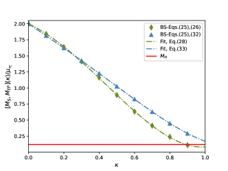
Figure 4: Pseudoscalar masses $M_{\Pi^{0}}(\kappa)/\mu_{tc}$(curve in light blue) and scalar masses depicted in Fig.(3). The contextualization of the curves behavior are described in the text.

V Conclusions

In this work, we verify that the effective potential responsible for $M_{S}\sim O(120)GeV$ behaves like $\propto\Phi^{4}$ at leading order. We also considered the comparison between two different approaches to obtain $M_{S}(\gamma)$, i.e. the effective potential for composite operators and Bethe-Salpeter equations. These results corroborate with the hypothesis that if the Higgs boson is a composite scalar, it may be a composite dilaton as suggested in Refs.[30, 31].

This result is displayed in Fig.(3), the curves obtained with different approaches, considering $G(k-q)$ given by Eq.(5), overlap exactly up to $\gamma\approx 1$. As we commented, the expansion considered in the Eq.(19) is not sensitive to the region of low momenta, which is captured by the BS equations, so that at $\gamma\approx 1$ the curves start to show different behaviors.

In the last section of this work, we include the determination of the lightest pseudo scalar mass $M_{\Pi^{0}}\approx 309GeV$, that confirms the estimate presented in Ref.[38]. Charged and colored technifermions will not only have larger masses than the neutral technifermion(N), but also more radiative corrections to their masses, and we can expect even larger masses for these colored and charged pseudo scalar bosons.

According to the discussion presented in Ref.[39], we still have other contributions to the effective Lagrangian, given by Eq.(19). These contributions are the ones coming from ordinary massive quarks and leptons that couple to the composite scalar boson $\Phi$. These contributions will be dominated by the heaviest fermion, the quark top, and will generate terms of order $\Phi^{3}$ and $\Phi^{4}$.

However, as we verified in this work the $\Phi^{4}$ contributions to $\tilde{\Omega}$ from massive fermions can be disregarded, the only exception is the contribution to $\Phi^{3}$ term, which is small but introduce some effect in the scalar mass calculation. If the Higgs boson is a composite particle it is still possible that its constituents are bounded by a non-Abelian gauge strong interaction, and we believe that combining different approaches can be useful for characterizing the properties of this possible composite state.

Appendix A The pseudo scalar components $\chi_{P(i)}^{(0,1)}$ in the BS equations

Assuming that each constituent, the (N) techniquarks, carries half of the momentum $\alpha=\beta=1/2$ , the different components of Eq.(32), $\chi_{P(i)}^{(0,1)}$ for $i=0..3$, are listed in the sequence

$$\chi^{(0)}_{P0}(x,p^{2})=3[(x-\frac{1}{4}p^{2}+m^{2})J_{1}]I_{P0}+\Delta\chi^{(0)}_{P0}\,,$$ (36)

where

$$I_{P0}=\frac{2}{3\pi}\int dyy\chi^{(0)}_{P0}K_{1}\,,$$ (37)

with $y=k^{2}/\Lambda^{2}$ and

$$K_{1}(x,y)=\frac{3}{16\pi^{2}}\int d\theta sen^{2}\theta G(x,y,cos\theta)\,,$$ (38)

$$J_{1}=\frac{2}{\pi}\int_{0}^{\pi}d\theta\frac{sen^{2}\theta}{D(p^{2},q^{2},pqcos\theta)}$$ (39)

and in the Eq.(39), we have

$$D(p^{2},q^{2},pqcos\theta)=\{(q+\frac{1}{2}p)^{2}+m^{2}\}\{(q-\frac{1}{2}p)^{2}+m^{2}\}.$$ (40)

Considering Taylor’s series expansion of $(q+\frac{1}{2}p)^{2}+m^{2}$ and $(q-\frac{1}{2}p)^{2}+m^{2}$ , keeping the first-order derivative terms for $m$, we have that the function $J_{1}$ can be written as

$$J_{1}=\frac{2}{c_{1}c_{4}+c_{2}c_{3}}\left[\frac{c_{2}}{D_{1}}+\frac{c_{4}}{D_{2}}+d_{1}\left(\frac{c_{1}}{D_{1}}-\frac{c_{3}}{D_{2}}\right)\right]$$ (41)

where, in our approximation with $\alpha=\beta=1/2$, we obtain

$$c_{1}=c_{3}=x+\frac{1}{4}p^{2}+m^{2}$$

$$c_{2}=c_{4}=1+2mm^{\prime}$$

and $m^{\prime}$ is the derivative of $m$ with respect to the momentum. In addition, as a consequence of $\alpha=\beta$

$$d_{1}=0$$

$$D_{1}=D_{2}=c_{1}+\sqrt{c_{1}^{2}-p^{2}xc_{2}^{2}}.$$

In Eq.(36) , the term $\Delta\chi^{(0)}_{P0}$ stands for corrections to the leading-order results for $\chi^{(0)}_{P0}$, that correspond to $\chi^{(0,1)}_{P1}$ , $\chi^{(0,1)}_{P2}$ and $\chi^{(0,1)}_{P3}$.

With the approximations considered, we have

$$\Delta\chi^{(0)}_{P0}=-\frac{2}{3\pi}mp^{2}J_{1}\int dyy\chi_{P1}^{(0)}(K_{1}+2yK_{3})+$$

$$\hskip 39.83368pt-\frac{4}{9\pi}p^{2}J_{3}\int dyy\chi_{P1}^{(0)}(3K_{1}-4yK_{3})+$$

$$\hskip 39.83368pt+\frac{2}{3\pi}p^{2}(J_{1}-J_{3})h(K_{6},K_{3},x,y)$$

$$\hskip 39.83368pt+\frac{2}{3\pi}\left[(x-\frac{1}{4}p^{2}+m^{2})((J_{1}-4J_{3})p^{2}\right]$$

$$\hskip 39.83368pt\times h(K_{7},K_{1},y),$$ (42)

where we define,

$$h(K_{6},K_{3},x,y)=\int dyy\chi_{P3}^{(0)}\left(2\sqrt{xy}K_{6}-\frac{8}{3}xyK_{3}\right)$$

$$h(K_{7},K_{1},y)=\int dyy^{2}\chi_{P0}^{(2)}\left(\frac{4}{3}K_{7}-K_{1}\right).$$ (43)

In the equation above, the lowest order terms $\chi_{P(1-3)}^{(0)}$ are given by

$$\chi_{P1}^{(0)}=\frac{mJ_{1}}{J_{1}(x-\frac{1}{4}p^{2}+m^{2})}\chi^{(0)}_{P0}\,\,,\,\,\chi_{P2}^{(0)}=0\,\,,\,\,\chi_{P3}^{(0)}=\frac{1}{2}\frac{J_{1}}{J_{1}(x-\frac{1}{4}p^{2}+m^{2})}\chi^{(0)}_{P0}.$$ (44)

While the higher order term, $\chi_{P0}^{(2)}$ is given by

$$\chi_{P0}^{(2)}=\frac{1}{xp^{2}}\frac{4(x-\frac{1}{4}p^{2}+m^{2})J_{3}-J_{1}}{J_{1}(x-\frac{1}{4}p^{2}+m^{2})}\chi^{(0)}_{P0}.$$ (45)

We are dealing with scalars(S) and pseudo scalars(PS) bosons with equal mass constituents and in this case we have simpler equations, compared to Ref.[43], that correspond to

$$J_{2}=0\,\,\,,\,\,\,J_{3}=\frac{1}{D_{1}^{2}}.$$ (46)

In the Eqs.(42-45), the kernels $K_{i}(x,y)$, with $i=3,6,7$ are given by

$$K_{3}(x,y)=\frac{3}{16\pi^{2}}\int d\theta\frac{sen^{4}\theta}{x+y-2\sqrt{xy}cos\theta}G(x,y,cos\theta),$$ (47)

$$K_{6}(x,y)=\frac{3}{16\pi^{2}}\int d\theta sen^{2}\theta cos\theta G(x,y,cos\theta),$$ (48)

$$K_{7}(x,y)=\frac{3}{16\pi^{2}}\int d\theta sen^{4}\theta G(x,y,cos\theta).$$ (49)

As in the determination of $M_{S}(\kappa)$, to obtain $M_{PS}(\kappa)$ we consider $G_{\rho\nu}$ in the Landau gauge given by Eq.(5), in addition we also consider the MAC hypothesis[40, 41]. Therefore, in this equation $G(x,y,cos\theta)=\mu^{2}G(k-q)^{2}$, with $G(k-q)$ given by Eq.(5), that leads to

$$\mu^{2}G(k-q)=\frac{\mu^{2}}{p^{2}+k^{2}-2pqcos\theta}=G(x,y,cos\theta).$$ (50)

References

- [1] ATLAS Collaboration, Phys. Lett. B 716, 1 (2012).
- [2] CMS Collaboration, Phys. Lett. B 716, 30 (2012).
- [3] S. Weinberg, Phys. Rev. D 19, 1277 (1979).
- [4] L. Susskind, Phys. Rev. D 20, 2619 (1979).
- [5] E. Farhi and L. Susskind, Phys. Rept. 74, 277 (1981).
- [6] K. D. Lane and M. V. Ramana, Phys. Rev. D 44, 2678 (1991).
- [7] T. W. Appelquist, J. Terning and L. C. R. Wijewardhana, Phys. Rev. Lett. 79, 2767 (1997).
- [8] Y. Aoki et al., Phys. Rev. D 85, 074502 (2012).
- [9] T. Appelquist, K. Lane and U. Mahanta, Phys. Rev. Lett. 61, 1553 (1988).
- [10] R. Shrock, Phys. Rev. D 89, 045019 (2014).
- [11] M. Kurachi and R. Shrock, JHEP 0612, 034 (2006).
- [12] R. Foadi, M. T. Frandsen, T. A. Ryttov and F. Sannino, Phys. Rev. D 76, 055005 (2007).
- [13] M. Jarvinen, C. Kouvaris and F. Sannino, Phys. Rev. D 78, 115010 (2008).
- [14] Karin Dissauer, Mads T. Frandsen, Tuomas Hapola, and Francesco Sannino , Phys. Rev. D87, 035005 (2013).
- [15] Ari Hietanen, Claudio Pica, Francesco Sannino, and Ulrik Ishj Sndergaard, Phys. Rev. D87, 034508 (2013).
- [16] T.Appelquist, G.T.Fleming, and E.T.Neil, Phys. Rev. Lett. 100, 171607 (2008).
- [17] T.Appelquist, G.T.Fleming, and E.T.Neil, Phys. Rev. D79, 076010 (2009).
- [18] T.Appelquist, R.C.Brower, G.T.Fleming, A. Hasenfratz, X.Y.Jin, J.Kiskis, E.T.Neil, J.C.Osborn, C.Rebbi, E.Rinaldi, D.Schaich, P. Vranas, E. Weinberg, and O. Witzel (Lattice Strong Dynamics (LSD) Collaboration), Phys. Rev. D 93, 114514 (2016).
- [19] Thomas Appelquist, James Ingoldby and Maurizio Piai, J. High Energ. Phys. (2017), 2017: 35; J. High Energ. Phys. (2018) 2018: 39.
- [20] V. A. Miransky and K. Yamawaki, Mod. Phys. Lett. A 4, 129 (1989).
- [21] K.-I. Kondo, H. Mino and K. Yamawaki, Phys. Rev. D 39, 2430 (1989).
- [22] V. A. Miransky, T. Nonoyama and K. Yamawaki, Mod. Phys. Lett. A 4, 1409 (1989).
- [23] T. Nonoyama, T. B. Suzuki and K. Yamawaki, Prog. Theor. Phys. 81, 1238 (1989).
- [24] V. A. Miransky, M. Tanabashi and K. Yamawaki, Phys. Lett. B 221, 177 (1989).
- [25] K.-I. Kondo, M. Tanabashi and K. Yamawaki, Mod. Phys. Lett. A 8, 2859 (1993).
- [26] T. Takeuchi, Phys. Rev. D 40, 2697 (1989).
- [27] B. Holdom, Phys. Rev. D 24, 1441 (1981).
- [28] K. Yamawaki, Prog. Theor. Phys. Suppl. 180, 1 (2010); and hep-ph/9603293; C. T. Hill, E. H. Simmons, Phys.Rept. 381 (2003) 235-402, Phys.Rept. 390 (2004) 553-554 (erratum); e-Print: hep-ph/0203079 [hep-ph].
- [29] B. Bellazzini, C. Csáki and J. Serra, Eur. Phys. J. C 74, 2766 (2014).
- [30] E. J. Eichten and K. Lane, Phys. Rev. D 103, 115022 (2021).
- [31] K. Lane, “The composite Higgs signal at the next big collider”, Snowmass Summer Study, arXiv: 2203.03710.
- [32] E. Gildener and S. Weinberg, Phys. Rev. D 13, 3333 (1976).
- [33] A. Doff and A. A. Natale, Int. J. Mod. Phys.A 38, 8, 2350046 (2023).
- [34] P. Maris, AIP Conference Proceedings 892, 65 (2007); Craig D. Roberts, David G. Richards, Tanja Horn and Lei Chang, Prog. Part. Nucl. Phys. 120, 103883 (2021); Pei-Lin Yin, Chen Chen, Gastão Krein, Craig D. Roberts, Jorge Segovia, and Shu-Sheng Xu, Phys. Rev. D 100, 034008 (2019).
- [35] J. M. Cornwall, R. Jackiw and E. Tomboulis, Phys. Rev. D 10, 2428 (1974).
- [36] J. M. Cornwall and R. C. Shellard, Phys. Rev. D 18, 1216 (1978)
- [37] A. A. Natale, Nucl. Phys. B 226, 365 (1983).
- [38] A. Doff, A. A. Natale, EPL 136, 5, 51002 (2021).
- [39] A. Doff, A. A. Natale and P. S. Rodrigues da Silva, Phys. Rev. D 77, 075012 (2008).
- [40] J. M. Cornwall, Phys. Rev. D 10, 500 (1974).
- [41] S. Raby, S. Dimopoulos, and L. Susskind, Nucl. Phys. B 169, 373 (1980).
- [42] P. Jain and H. J. Munczek, Phys. Rev. D 44, 1873 (1991).
- [43] H. J. Munczek and P. Jain, Phys. Rev. D 46, 438 (1992).
- [44] P. Jain and H. J. Munczek, Phys. Rev. D 48, 5403 (1993).
- [45] R. Delbourgo and M. D. Scadron, Phys. Rev. Lett. 48, 379 (1982).
- [46] K. Lane, Phys. Rev. D 10, 2605 (1974).
- [47] A. Doff, A. A. Natale, Eur. Phys. J. C 32, 417 (2003).