Determination of stable branches of relative equilibria of the $N$-vortex problem on the sphere

Abstract

We consider the $N$-vortex problem on the sphere assuming that all vorticities have equal strength. We investigate relative equilibria (RE) consisting of $n$ latitudinal rings which are uniformly rotating about the vertical axis with angular velocity $\omega$. Each such ring contains $m$ vortices placed at the vertices of a concentric regular polygon and we allow the presence of additional vortices at the poles. We develop a framework to prove existence and orbital stability of branches of RE of this type parametrised by $\omega$. Such framework is implemented to rigorously determine and prove stability of segments of branches using computer-assisted proofs. This approach circumvents the analytical complexities that arise when the number of rings $n\geq 2$ and allows us to give several new rigorous results. We exemplify our method providing new contributions consisting in the determination of enclosures and proofs of stability of several equilibria and RE for $5\leq N\leq 12$.

Keywords: $N$-vortex problem, relative equilibrium, stability, interval arithmetic, computer-assisted proofs.
2020 MSC: 70K42, 76M60, 65G30, 65G20, 47H10, 37C25.

1 Introduction

In the last decades the $N$-vortex problem on the sphere has received considerable attention. A non-exhaustive list of references contains [11, 10, 32, 44, 13, 61, 12, 45, 64, 16, 24, 54] and other papers that are mentioned below. The equations of motion go back to Gromeka [27] and Bogomolov [9]. The importance of the system is usually associated with geophysical fluid dynamics since it provides a simple model for the dynamics of cyclones and hurricanes in planetary atmospheres. Moreover, recent numerical work [46] suggests that the $N$-vortex problem on the sphere plays a crucial role in the long term behaviour of the incompressible two-dimensional Euler equations on the same domain. We also mention that the $N$-vortex problem on the sphere equipped with a general Riemannian metric was recently studied in [65] and, as noted in [34, 58], this is a convenient approach to treat the $N$-vortex problem on more general closed surfaces of genus $0$. We refer the reader to the book [53] and the papers [1, 2] for an overview and extensive bibliography on vortex dynamics.

The equations of motion of the problem define a Hamiltonian system on the $2N$-dimensional phase space $M$ which is obtained as the cartesian product of $N$ copies of the 2-sphere $S^{2}$ minus the collision set. The Hamiltonian function $H:M\to\mathbb{R}$ accounts for the pairwise interaction between the vortices, and the symplectic form $\Omega$ on $M$ is a weighted sum by the vortex strengths of the area form on each copy of $S^{2}$. A fundamental aspect of the problem is that both $H$ and $\Omega$ are invariant under the action of $SO(3)$ on $M$ that simultaneously rotates all vortices. As a consequence, the equations of motion are $SO(3)$-equivariant and, in accordance with Noether’s Theorem, there exists a momentum map $\Phi:M\to\mathbb{R}^{3}$, whose components are first integrals. It is well-known (see e.g. [47]) that the problem is integrable if $N\leq 3$, and on the zero level set of $\Phi$ if $N=4$, and appears to be non-integrable otherwise.

The simplest solutions to the problem are the equilibrium configurations which correspond to the critical points of $H$. If all the vortex strengths have the same sign, then $H$ is bounded from below and it assumes a global minimum on $M$. The minimising configurations are called ground states and form a very important kind of stable equilibria. Unfortunately, the rigorous determination of the ground states is an extremely complicated problem for which very little is known. If all vortices have equal strengths, which is the case that we treat in most of this work, after a suitable normalisation, the Hamiltonian $H:M\to\mathbb{R}$ becomes

$$H(v)=-\sum_{i<j}\ln\left(\left\|v_{i}-v_{j}\right\|^{2}\right),\qquad v=(v_{1},\dots,v_{N})\in M,$$

where, for all $i=1,\dots,N$, $v_{i}$ is a unit vector on $\mathbb{R}^{3}$ which specifies the position of the $i^{th}$ vortex on the unit sphere $S^{2}$ (note that $v_{i}\neq v_{j}$ for all $i$, $j$, since collisions have been removed). Using the above expression for $H$, it is easy to see that the ground state configurations are geometrically characterised as those which maximise the product of the pairwise euclidean distances between the vortices. These configurations are sometimes called Fekete points, and their determination corresponds to Smale’s problem $\#7$ which has only been solved for a few values of $N$ (2, 3, 4, 5, 6 and 12). We refer the reader to [3], the nice review [4] and the references therein for more information on Smale’s problem $\#7$. In Table 1.1 below we list the known Fekete points together with a conjecture of their position for the values $N=7,\dots,11$ (the detailed description of the configurations in the table is given in section 6.1). The configurations of the table are illustrated in Figures 1.1 and 1.2. One can analytically show that these are critical points of $H$ except for $N=11$ whose treatment, as explained in section 6.1, required the use of a computer-assisted proof.

$N$	Polyhedron	$\mathbb{Z}_{m}$ -symmetries
2	antipodal points	$\mathbb{Z}_{2}$
3	equilateral triangle	$\mathbb{Z}_{3}$
4	tetrahedron	$\mathbb{Z}_{2}$ and $\mathbb{Z}_{3}$
5	triangular bipyramid	$\mathbb{Z}_{2}$ and $\mathbb{Z}_{3}$
6	octahedron	$\mathbb{Z}_{2}$, $\mathbb{Z}_{3}$ and $\mathbb{Z}_{4}$
7	pentagonal bipyramid	$\mathbb{Z}_{2}$ and $\mathbb{Z}_{5}$
8	square antiprism	$\mathbb{Z}_{2}$ and $\mathbb{Z}_{4}$
9	triaugmented triangular prism	$\mathbb{Z}_{2}$ and $\mathbb{Z}_{3}$
10	gyroelongated square bipyramid	$\mathbb{Z}_{2}$ and $\mathbb{Z}_{4}$
11	–     (see section 6.1 for details)	$\mathbb{Z}_{2}$
12	icosahedron	$\mathbb{Z}_{2}$, $\mathbb{Z}_{3}$ and $\mathbb{Z}_{5}$

Table 1.1: Known ($N=2,3,4,5,6,12$) and conjectured ($N=7,8,9,10,11$) ground states of the $N$ vortex problem on the sphere assuming identical vortex strengths. See section 6.1 for details.

Another type of fundamental solutions, whose study is the main topic of this work, is given by relative equilibria (RE). For our specific problem, these are periodic solutions in which all vortices rotate uniformly about a fixed axis at constant angular speed $\omega\in\mathbb{R}$. These solutions correspond to critical points of $H$ restricted to the level sets of $\Phi$. Without loss of generality, the rotation axis is chosen as the vertical $z$-axis in $\mathbb{R}^{3}$ throughout this work.

An important class of RE is that in which the vortices are arranged in $n$ latitudinal rings, each of which consists of a regular polygon of $m$ identical vortices. We allow for the possibility of having $p$ vortices at the poles ($p=0,1$ or $2$) so the total number of vortices $N=mn+p$. Such RE possess a discrete $\mathbb{Z}_{m}$-symmetry and will be thus called $\mathbb{Z}_{m}$-symmetric RE. Several previous works have focused on the study of this type of RE [57, 13, 41, 39, 15, 7, 40]. In particular, the seminal work of Lim, Montaldi and Roberts [41] gives several existence results based on symmetry considerations. However, explicit analytic expressions and stability results for these RE are mainly known for the case of $n=1$ ring (see [40] for a comprehensive list of results in this case). When the number of rings $n\geq 2$, the computational complexity enormously increases and one has to settle with numerical investigations as in [40]. This is somewhat unsettling, considering that the $\mathbb{Z}_{m}$-symmetric RE consisting of only one ring lose stability as the number of vortices $m$ in each ring grows (see e.g. [40] and our discussion in section 6.3 for precise statements).

In this work we circumvent the difficulty to obtain rigorous existence and stability results for $\mathbb{Z}_{m}$-symmetric RE having $n\geq 2$ rings by relying on computer-assisted proofs (CAPs). This approach falls in the category of CAPs in dynamics, which is by now a well-developed field, with some famous early pioneering works being the proof of the universality of the Feigenbaum constant [38] and the proof of existence of the strange attractor in the Lorenz system [62]. We refer the interested reader to the survey papers [33, 50, 59, 5, 26, 30], as well as the books [63, 6, 51].

1.1 Contributions

Our work focuses on the case of equal vortex strengths and develops a theoretical framework for existence and stability of branches of $\mathbb{Z}_{m}$-symmetric RE parametrised by the angular speed $\omega$. This framework is implemented in an INTLab code (available in [20]) which establishes existence and provides rigorous bounds for (segments of) the branch using CAPs. Moreover, the code also performs a (nonlinear) stability test which may be validated with a CAP.

The input for the code is a numerical approximation of a non-degenerate RE (configuration and angular speed) with a prescribed $\mathbb{Z}_{m}$-symmetry. Provided that the given RE approximation has sufficient precision and is far from bifurcations, the code returns an enclosure of a segment of the branch containing the approximated RE and possessing the prescribed symmetry. The stability procedure involves validation of the positivity of the spectrum of a certain matrix and limitations arise in the presence of eigenvalues which are either too close to zero or which cluster.

The fundamental aspects of our theoretical framework and its CAP-implementation are summarised below. We divide the presentation of our results on existence, stability and CAPs.

Existence.

The first step in our construction is to perform a discrete reduction of the system by $\mathbb{Z}_{m}$ leading to a reduced Hamiltonian system with an $SO(2)$-symmetry. This is the content of Theorem 3.5 whose formulation is inspired by the previous work [25] of the second and third author. This discrete reduction relies on the permutation symmetry of the vortices and corresponds to the restriction of the dynamics to the invariant submanifold of $M$ formed by $\mathbb{Z}_{m}$-symmetric configurations. Theorem 3.5 shows that the dynamics in this invariant manifold is conjugate to the dynamics of a symplectic Hamiltonian system on a $2n$-dimensional reduced phase space, that we denote $M_{n}$, and whose reduced Hamiltonian function $h:M_{n}\to\mathbb{R}$ is given explicitly by (3.4). Moreover, the theorem also shows that this reduced Hamiltonian system possesses an $SO(2)$-symmetry corresponding to the simultaneous rotation of the rings.

The discrete reduction allows us to cast the problem of determination of branches of $\mathbb{Z}_{m}$-symmetric RE parametrised by $\omega$ in terms of the determination of branches of critical points of the augmented Hamiltonian of the reduced system, which is the function $h_{\omega}:M_{n}\to\mathbb{R}$ depending parametrically on $\omega$ given by $h_{\omega}=h-\omega\phi$, where $\phi:M_{n}\to\mathbb{R}$ is the momentum map of the $SO(2)$-action on $M_{n}$. After introducing Lagrange multipliers to embed $M_{n}$ in $\mathbb{R}^{3n}$, and introducing an unfolding parameter as in [49, 29] to deal with an $SO(2)$-degeneracy coming from the symmetries, we reduce the problem of determining critical points of $h_{\omega}$ to finding zeros of a suitable map

$$F:\mathbb{R}^{d+1}\to\mathbb{R}^{d},\qquad(x,\omega)\mapsto F(x,\omega).$$ (1.1)

The map $F$ involves the derivatives of $h_{\omega}$ and its explicit form, and the dimension $d$, may be read from (3.15). Under the hypothesis that a non-degenerate zero of $F$ is known (corresponding to a $\mathbb{Z}_{m}$-symmetric RE of our problem which is non-degenerate in a sense that we make precise in the text) the existence of a local branch of $\mathbb{Z}_{m}$-symmetric RE parametrised by $\omega$ is then guaranteed by the implicit function theorem. The existence results that we have just outlined are formalised in Theorem 3.10 and Corollary 3.12. In particular, the corollary implies the existence of local branches of $\mathbb{Z}_{m}$-symmetric RE emanating from each $\mathbb{Z}_{m}$-symmetry of the equilibria illustrated in Figures 1.1 and 1.2 having $N\neq 7$. These RE are obtained via a suitable vertical displacement of the rings, which results in their uniform rotation with small angular frequency about the vertical axis.

Finally we indicate that this paper also contains an original general existence result which is not used in our framework but provides a groundwork for our investigation. It is valid for arbitrary vortex strengths and shows existence of two local branches of RE parametrised by $\omega$ emanating from any non-degenerate equilibrium (Theorem 3.2).

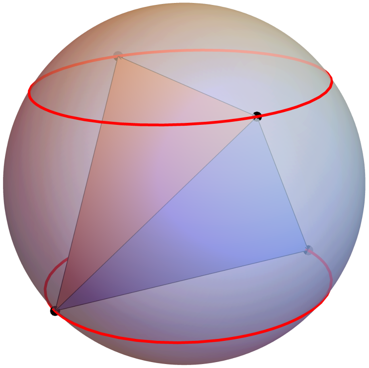
(a) $N=4$, $\mathbb{Z}_{2}$

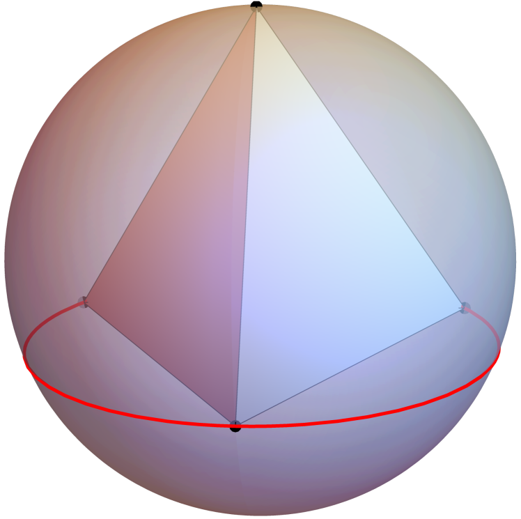
(b) $N=4$, $\mathbb{Z}_{3}$

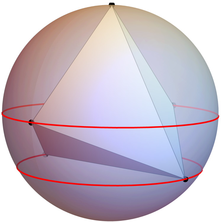
(c) $N=5$, $\mathbb{Z}_{2}$

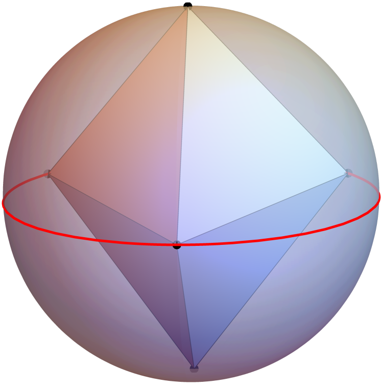
(d) $N=5$, $\mathbb{Z}_{3}$

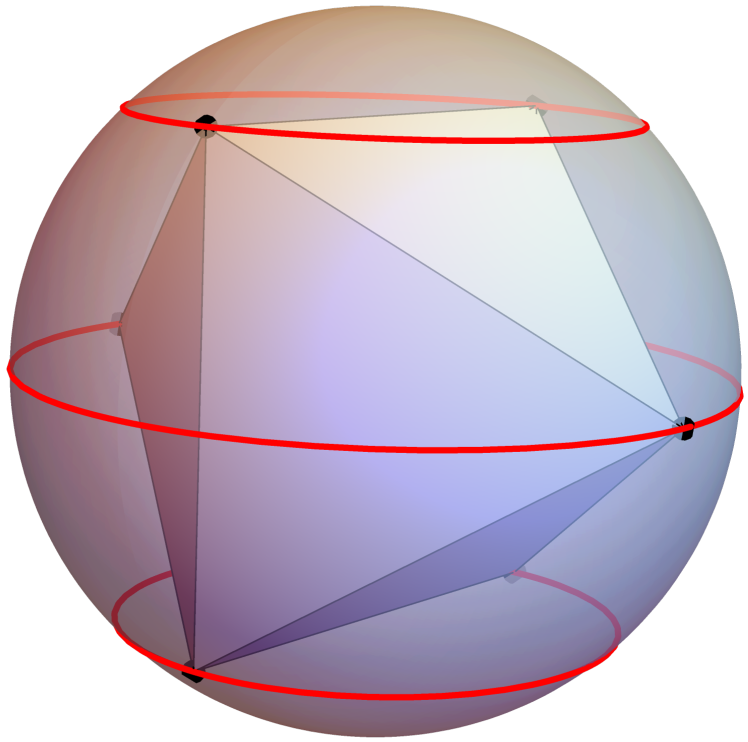
(e) $N=6$, $\mathbb{Z}_{2}$

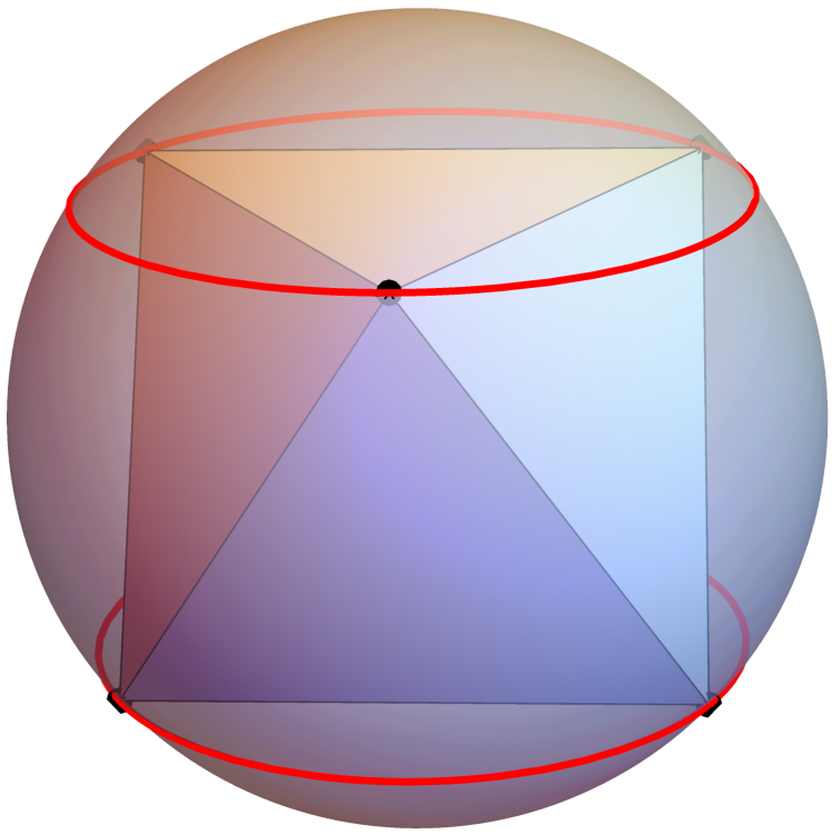
(f) $N=6$, $\mathbb{Z}_{3}$

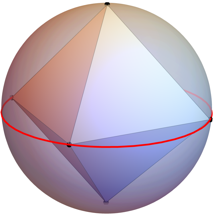
(g) $N=6$, $\mathbb{Z}_{4}$

(h) $N=12$, $\mathbb{Z}_{2}$

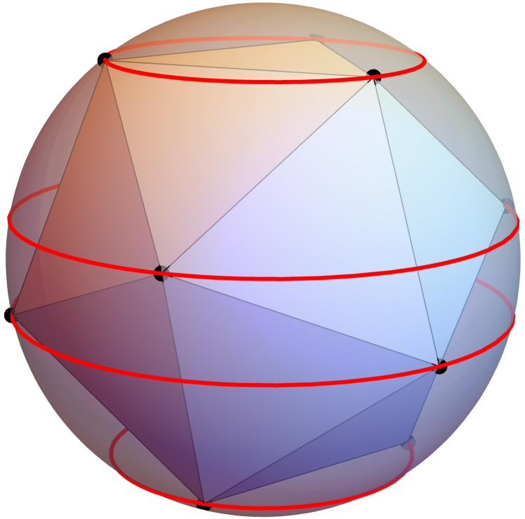
(i) $N=12$, $\mathbb{Z}_{3}$

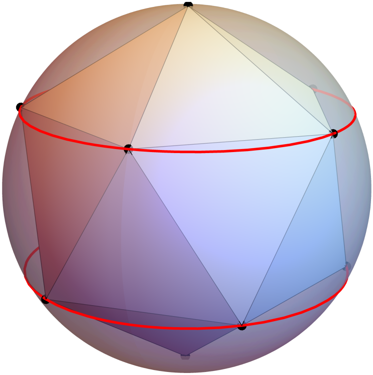
(j) $N=12$, $\mathbb{Z}_{4}$

Figure 1.1: Ground states for $N=4,5,6,12$ and their $\mathbb{Z}_{m}$-symmetries.

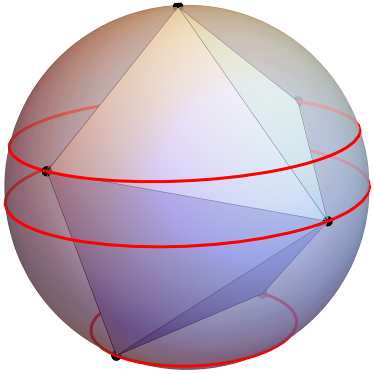
(a) $N=7$, $\mathbb{Z}_{2}$

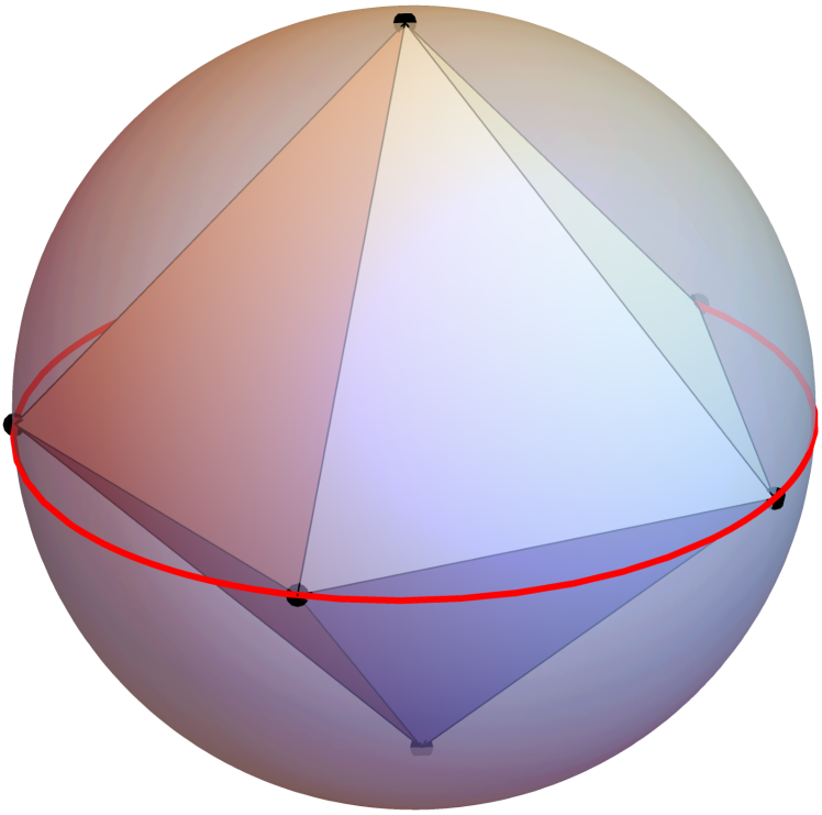
(b) $N=7$, $\mathbb{Z}_{5}$

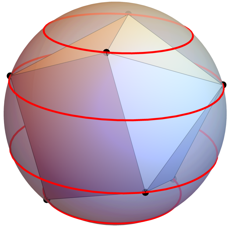
(c) $N=8$, $\mathbb{Z}_{2}$

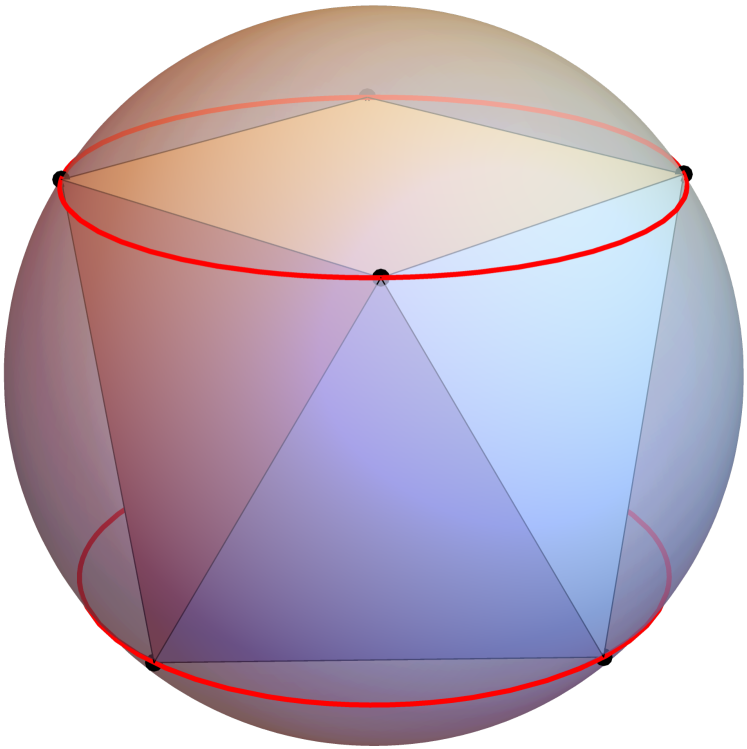
(d) $N=8$, $\mathbb{Z}_{4}$

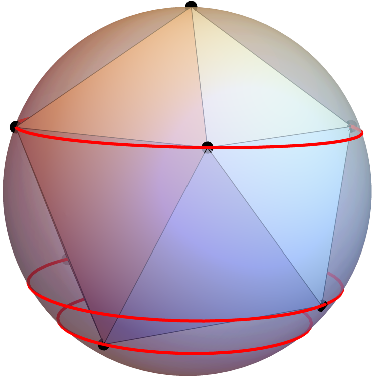
(e) $N=9$, $\mathbb{Z}_{2}$

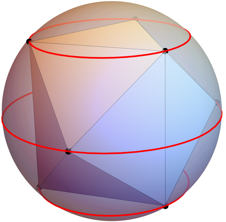
(f) $N=9$, $\mathbb{Z}_{3}$

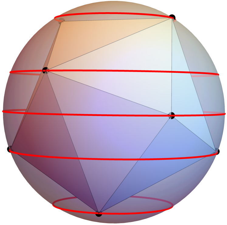
(g) $N=10$, $\mathbb{Z}_{2}$

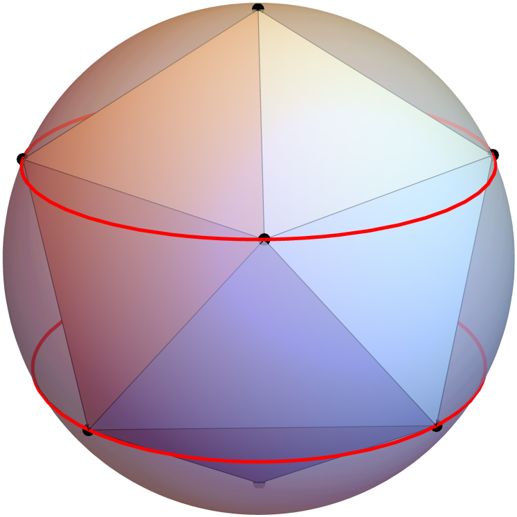
(h) $N=10$, $\mathbb{Z}_{4}$

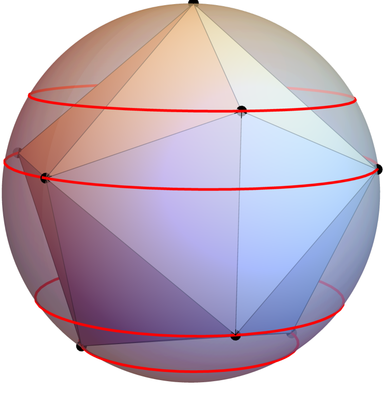
(i) $N=11$, $\mathbb{Z}_{2}$

Figure 1.2: Conjectured ground states for $N=7,8,9,10,11$ and their $\mathbb{Z}_{m}$-symmetries.

Stability.

Our nonlinear stability analysis relies on the energy-momentum method of Patrick [56]. Such method concludes Lyapunov stability modulo a subgroup, which in our case generically translates into orbital stability of a periodic orbit (see Proposition 2.7). The method examines positivity of a certain Hessian matrix which we block-diagonalise exploiting the $\mathbb{Z}_{m}$-symmetries following closely the construction of Laurent-Polz, Montaldi and Roberts [40]. Our approach differs from [40] in two ways. On the one hand, instead of using spherical coordinates, we work with the extrinsic geometry induced by our embedding of $M$ on $\mathbb{R}^{3N}$. This allows us to interpret tangent vectors to $M$ as vectors in the ambient space $\mathbb{R}^{3N}$, which is convenient for the implementation of CAPs. Secondly, we refine the block diagonalisation of [40] by exploiting the complex structure of some blocks as determined by Theorem 4.8. The great technicality involved in this block diagonalisation and its refinement is compensated by obtaining larger ranges of application of CAPs, since the method prevents clustering of eigenvalues of large matrices.

A summary of the stability test which indicates the matrix blocks which need to be computed, and their dimension, according to the values of $m$, $n$ and $p$ is given in subsection 4.5.

Computer-assisted proofs (CAPs).

The CAPs in this paper are obtained via a finite dimensional Newton-Kantorovich like theorem (see [55] for the original version), which is similar to the well-known interval Newton’s method [28, 48] and Krawczyk’s operator approach [35, 52]. This method allows us to find zeros of the mapping $F$ in (1.1) to find enclosures of the branches of $\mathbb{Z}_{m}$-symmetric RE and also, via a suitable formulation, to validate eigenvalues necessary for the stability test.

As mentioned above, the CAPs are implemented in an INTLab code available in [20], whose input is a numerical approximation of a $\mathbb{Z}_{m}$-symmetric RE (configuration and angular speed). If the approximation has sufficient precision and is not too close to a bifurcation, the code proves existence of a branch of RE with this symmetry, determines an enclosure and validates the stability test.

The range of applications of our framework and our code is exemplified by the results presented in section 6. In particular, Theorem 6.1 proves stability of the equilibrium configurations in Table 1.1 for $N=8,9,10,11$ (the case $N=7$ is degenerate and our test is inconclusive, and the stability for other values of $N$ in the table was known). We then prove existence and find enclosures of segments of stable branches of RE emanating from the equilibria in Table 1.1. These results are presented in section 6.2, and allow us to conjecture which branches of RE minimise $H$ on the level sets $\Phi^{-1}(\mu)\subset M$ for $\mu$ close to zero for the different values of $N$. Finally, in section 6.3, we investigated RE near total collision. The results of [40] imply that for $N\geq 10$ the $\mathbb{Z}_{m}$-symmetric RE consisting of only 1-ring are unstable. Our results in section 6.3 provide an educated first guess of the shape of the RE which minimises $H$ on the level sets of $\Phi$ near total collision for $N=10,11,12$.

1.2 Structure of the paper

We start by reviewing some known preliminary material in section 2. This serves to introduce concepts and notation used throughout the paper. Moreover, it is useful to recall known details and results on RE, the energy-momentum method and the CAPs that we use. We then focus on results on existence of branches of RE in section 3. Our main original results in this section are Theorem 3.2 on the existence of branches of RE near equilibrium for arbitrary vortex strengths, Theorem 3.5 on the discrete $\mathbb{Z}_{m}$-reduction in the case of equal vorticities, and Theorem 3.10 and Corollary 3.12 on the existence of local branches of $\mathbb{Z}_{m}$-symmetric RE. Section 4 focuses on the application of the energy-momentum method for nonlinear stability of RE. Most of this section is a development of the block-diagonalisation of [40] which, as mentioned above, is better suited for the implementation of CAPs. Our refinement of this construction is given in Theorem 4.8 which exploits the complex structure of some blocks. A useful summary of the blocks that need to be constructed and whose eigenvalues need to be calculated according to the values of $m$, $n$ and $p$ is given in subsection 4.5. In Section 5 we explain how CAPs are implemented using the setting of sections 3 and 4 to establish existence and stability of branches of $\mathbb{Z}_{m}$-symmetric RE. Finally, we give examples of the range of applications of our framework and our code in section 6. The paper contains a series of appendices which complement the main body of the text.

2 Preliminaries

In this section we recall the equations of motion and basic known properties of the equations of motion of the $N$-vortex on the sphere. This allows us to introduce the notation and concepts used ahead. In particular our working definition of RE is given in Definition 2.1. We then recall some properties of RE which follow from the general theory of RE for Hamiltonian systems with symmetry which are used in our construction. We also recall the energy momentum method for nonlinear stability in subsection 2.4 and the Newton-Kantorovich like theorem for our CAPs in subsection 2.5.

2.1 Equations of motion

The equations of motion of the $N$-vortex problem on the sphere are a Hamiltonian system on the phase space $M$ obtained as the cartesian product of $N$ copies of the unit sphere in $\mathbb{R}^{3}$ minus the collision set $\Delta$. That is, $M:=(S^{2}\times\dots\times S^{2})\setminus\Delta$ where

$$S^{2}:=\{w\in\mathbb{R}^{3}\,:\,\|w\|=1\}\qquad\mbox{and}\qquad\Delta:=\{(v_{1},\dots,v_{N})\in M\,:\,v_{i}=v_{j}\,\,\mbox{for some $i\neq j$}\}.$$

The Hamiltonian function $H:M\to\mathbb{R}$ and symplectic form $\Omega$ on $M$ are given by

$$H(v):=-\frac{\Gamma_{i}\Gamma_{j}}{4\pi}\sum_{i<j}\ln\left(\left\|v_{i}-v_{j}\right\|^{2}\right),\qquad\Omega:=\sum_{i=1}^{N}\Gamma_{i}\pi^{*}_{i}\omega_{S^{2}}.$$

Here $v=(v_{1},\dots,v_{N})\in M$ specifies the position of each of the vortices whose respective (constant) intensities are denoted by the scalars $\Gamma_{i}\neq 0$. The map $\pi_{i}:M\to S^{2}$ denotes the projection onto the $i^{th}$ factor of the cartesian product $S^{2}\times\dots\times S^{2}$ and $\omega_{S^{2}}$ is the standard area form on $S^{2}$. The resulting equations of motion are

$$\dot{v}_{j}=-\frac{1}{\Gamma_{j}}v_{j}\times\nabla_{v_{j}}H=\frac{1}{4\pi}\sum_{i\neq j}\Gamma_{i}\frac{v_{i}\times v_{j}}{\|v_{i}-v_{j}\|^{2}},\qquad i=1,\dots,N,$$ (2.1)

where $\times$ denotes the cross product in $\mathbb{R}^{3}$. Owing to the Hamiltonian structure, the Hamiltonian function $H$ is a first integral.

2.2 Rotational symmetries, center of vorticity, equilibria and relative equilibria

Rotational symmetries.

The position of the vortices in the sphere is specified by $v=(v_{1},\dots,v_{N})\in M$. This tacitly assumes a choice of an inertial frame whose origin lies at the center of the sphere which defines cartesian coordinates for the $v_{j}$’s. There is freedom in the choice of orientation of this inertial frame and this is reflected by the invariance of the problem under the $SO(3)$ action that simultaneously rotates all vortices. Specifically we consider the $SO(3)$ action on $M$ defined by

$$(g,v)\mapsto g.v:=(gv_{1},\dots,gv_{N})\in M,\qquad g\in SO(3),\;v=(v_{1},\dots,v_{N})\in M.$$

For $N\geq 3$ this action is free since the collisions do not belong to $M$. It is also a proper action since $SO(3)$ is compact.

It is easily checked that both the Hamiltonian and the symplectic form are invariant under this action and as a consequence, the equations of motion (2.1) are $SO(3)$-equivariant.

Center of vorticity.

One may easily show that the components of the map

$$\Phi:M\to\mathbb{R}^{3},\qquad\Phi(v)=\Gamma_{1}v_{1}+\dots+\Gamma_{N}v_{N},$$ (2.2)

are first integrals of the equations of motion (2.1). It is common to refer to $\Phi(v)$ as the center of vorticity of the vortex configuration $v=(v_{1},\dots,v_{N})$. The existence of these first integrals is in fact an instance of Noether’s theorem. Upon the standard identification of the dual Lie algebra $\mathfrak{so}(3)^{*}$ with $\mathbb{R}^{3}$, the function $\Phi$ can be geometrically interpreted as the momentum map associated to the symplectic action of $SO(3)$ on the symplectic manifold $(M,\Omega)$.

For $N\geq 3$, the freeness of the action guarantees that $\Phi$ is a submersion onto its image. As a consequence, if $\mu\in\mathbb{R}^{3}$ is such that $\Phi(v)=\mu$ for some $v\in M$, then $\Phi^{-1}(\mu)$ is a smooth submanifold of $M$ of codimension 3 and $T_{v}\Phi^{-1}(\mu)=\ker d\Phi(v)$.

The momentum map $\Phi$ plays a fundamental role in the study of relative equilibria. An important property of $\Phi$ is its equivariance with respect to the coadjoint representation which, in our interpretation, is simply the standard linear action of $SO(3)$ on $\mathbb{R}^{3}$, namely, one has

$$\Phi(g.v)=g\Phi(v),\quad\forall v\in M,\;g\in SO(3).$$ (2.3)

Equilibrium points and ground states.

The simplest solutions of the equations of motion are the equilibria which are in one-to-one correspondence with the critical points of $H:M\to\mathbb{R}$. Due to the $SO(3)$ invariance of the problem, equilibrium points are never isolated: if $v_{0}\in M$ is an equilibrium of (2.1) so is $g.v_{0}$ for any $g\in SO(3)$. In other words, the orbit $SO(3).v_{0}\subset M$ is comprised of equilibrium points.

If all the vortex strengths $\Gamma_{i}$ have the same sign, then $H$ is bounded from below and it assumes a global minimum on $M$. The minimising configurations are called ground states and form a very important kind of equilibria from the physical point of view. Again, the $SO(3)$-invariance of $H$ implies that if $v_{0}\in M$ is a ground state then the orbit $SO(3).v_{0}\subset M$ consists of ground states. The ground states of the system are stable in a sense that will be made precise below. As mentioned in the introduction, proving that a given equilibrium is the ground state of the system is a very difficult problem for which very little is known.

Relative equilibria.

The next type of fundamental solutions are the so-called relative equilibria (RE) which are the main subject of this work. This kind of solutions may exist for any system of differential equations which is equivariant with respect to the action of a continuous symmetry group. There are several equivalent definitions of relative equilibria. For our purposes, it suffices to define them as solutions of the equations that at the same time are orbits of a one-parameter subgroup of the symmetry group. Thus, in our case, relative equilibria have the form $v(t)=e^{\xi t}.a$ for a fixed $a\in M$ and a skew-symmetric matrix $\xi\in\mathfrak{so}(3)$. This is a periodic solution in which the vortices steadily rotate along the axis passing through the center of the sphere in the direction of the vector $\xi_{e}\in\mathbb{R}^{3}$ satisfying $\langle\xi_{e}\rangle=\ker\xi$ and whose angular velocity $\omega_{e}$ satisfies $2\omega_{e}^{2}=\mbox{trace}(\xi\xi^{T})$.

Just like equilibrium points, relative equilibria are never isolated: if $v(t)=e^{\xi t}.a$ is a relative equilibrium and $g\in SO(3)$ then, by equivariance of (2.1), $\tilde{v}(t):=g.v(t)$ is also a solution. However, we may write

$$\tilde{v}(t)=g.v(t)=(ge^{\xi t}g^{-1}).(g.a)=e^{(g\xi g^{-1})t}.(g.a)=e^{\tilde{\xi}t}.\tilde{a},$$

where $\tilde{\xi}:=g\xi g^{-1}\in\mathfrak{so}(3)$ and $\tilde{a}:=g.a\in M$, which shows that $\tilde{v}(t)$ is also a relative equilibrium with axis of rotation $\tilde{\xi}_{e}=g\xi_{e}$ and the same angular frequency $\tilde{\omega}_{e}=\omega_{e}$. Physically, this means that the orientation of the axis of rotation of a relative equilibrium is unessential and may be arbitrarily chosen via a suitable rotation of the inertial frame. On the other hand, relative equilibria having distinct angular frequencies are not related by a rotation. Therefore, for the rest of the paper, we will restrict our attention to relative equilibria for which the axis of rotation is the $z$-axis and we will give a prominent role to the angular velocity $\omega$. In accordance with this, we search for solutions of (2.1) of the form

$$v(t)=e^{\omega J_{3}t}.a=(e^{\omega J_{3}t}a_{1},\dots,e^{\omega J_{3}t}a_{N}),\qquad J_{3}:=\begin{pmatrix}0&-1&0\\ 1&0&0\\ 0&0&0\end{pmatrix},$$ (2.4)

for a certain frequency $\omega\in\mathbb{R}$ and a configuration $a=(a_{1},\dots,a_{N})\in M$. Our discussion leads to the following definition.

Definition 2.1.

A relative equilibrium (RE) of the equations of motion (2.1) is a pair $(a,\omega)\in M\times\mathbb{R}$ such that $v(t)$ given by (2.4) is a solution of (2.1). We say that $\omega$ is the angular velocity and $a\in M$ is the configuration of the relative equilibrium.

Remark 2.2.

1. Equilibrium points may be interpreted as RE with zero angular velocity.

2. If $(a,\omega)$ is a RE with $\omega\neq 0$, then so is $(e^{J_{3}\theta}.a,\omega)$ for any $\theta\in[0,2\pi)$. This is a consequence of the autonomous nature of the equations of motion (2.1): if $v(t)$ is a solution, then so is $v(t+t_{0})$ for any $t_{0}\in\mathbb{R}$. In other words, $a$ is determined up to a time-shift along the solution with initial condition $a$. Considering that the solution is periodic, this time-shift corresponds to a certain $SO(2)$ action. Such $SO(2)$ action is precisely the one-parameter subgroup of $SO(3)$ of rotations about the $z$ axis. Namely, if we denote $e_{3}:=(0,0,1)\in\mathbb{R}^{3}$, and define

   $$SO(2):=\{g\in SO(3)\,:\,ge_{3}=e_{3}\}=\left\{e^{J_{3}\theta}=\begin{pmatrix}\cos\theta&-\sin\theta&0\\ \sin\theta&\cos\theta&0\\ 0&0&1\end{pmatrix}\,:\,\theta\in[0,2\pi)\right\},$$ (2.5)

   then the orbit $SO(2).a$ coincides with the dynamical orbit of the solution $v(t)=e^{\omega J_{3}t}.a$, and is comprised of relative equilibrium configurations with the same angular velocity $\omega$.

3. Some authors instead define the whole orbit $SO(3).a\subset M$ of the relative equilibrium configuration $a$ as the relative equilibrium since it projects to a single equilibrium point of the reduced system on the quotient space $M/SO(3)$. As explained in item (ii), our approach selects instead an $SO(2)$-orbit of representatives. This is essential for the continuation of relative equilibria as a function of the angular velocity $\omega$ considered ahead.

For any $\omega\in\mathbb{R}$ define the augmented Hamiltonian

$$H_{\omega}:M\to\mathbb{R},\qquad H_{\omega}(v):=H(v)-\omega\Phi_{3}(v),$$ (2.6)

where $\Phi_{3}:M\to\mathbb{R}$ denotes the third component of the momentum map $\Phi$ given by (2.2). Namely, $\Phi_{3}(v)=e_{3}\cdot\Phi(v)$ where $e_{3}=(0,0,1)\in\mathbb{R}^{3}$, and $\cdot$ denotes the standard euclidean product in $\mathbb{R}^{3}$. The following proposition is a particular instance of general results on relative equilibria on symplectic manifolds (see e.g. [42]). We present an elementary proof for completeness.

Proposition 2.3.

The following statements hold.

1. $(a,\omega)\in M\times\mathbb{R}$ is a relative equilibrium if and only if $a\in M$ is a critical point of $H_{\omega}$.

2. If $(a,\omega)\in M\times\mathbb{R}$ is a relative equilibrium with $\omega\neq 0$ then $e_{3}\times\Phi(a)=0$.

Proof.

(i) Let $\omega\in\mathbb{R}$ and introduce the time dependent change of variables,

$$y_{j}(t)=e^{-\omega J_{3}t}v_{j}(t)\text{,}\qquad j=1,\dots,N.$$

According to Definition 2.1, it is clear that $(a,\omega)\in M\times\mathbb{R}$ is a relative equilibrium if and only if $a\in M$ is an equilibrium solution for the equations satisfied by $y(t)=(y_{1}(t),\dots,y_{N}(t))$. A direct calculation shows that

$$\dot{y}_{j}=\frac{1}{4\pi}\sum_{i\neq j)}^{N}\Gamma_{i}\frac{y_{i}\times y_{j}}{\left\|y_{j}-y_{i}\right\|^{2}}-\omega e_{3}\times y_{j}=-y_{j}\times\left(\nabla_{y_{j}}H_{\omega}(y)\right).$$

This shows that the equations for $y(t)$ are Hamiltonian on the symplectic manifold $(M,\Omega)$ with respect to the Hamiltonian function $H_{\omega}$. As a consequence, the equilibrium points of $y(t)$ are in one-to-one correspondence with the critical points of $H_{\omega}$.

(ii) By conservation of $\Phi$ we have $\Phi(a)=\Phi(v(t))$ where $v(t)$ is given by (2.4). Therefore,

$$\begin{split}\Gamma_{1}a_{1}+\dots+\Gamma_{N}a_{N}&=\Gamma_{1}e^{\omega J_{3}t}a_{1}+\dots+\Gamma_{N}e^{\omega J_{3}t}a_{N}\\ &=e^{\omega J_{3}t}(\Gamma_{1}a_{1}+\dots+\Gamma_{N}a_{N})=e^{\omega J_{3}t}\Phi(a).\end{split}$$

Differentiating with respect to $t$ and evaluating at $t=0$ gives $\omega J_{3}\Phi(a)=0$, which for $\omega\neq 0$ is equivalent to $e_{3}\times\Phi(a)=0$.

∎

A fundamental observation which follows directly from (2.3) and the definition of the augmented Hamiltonian $H_{\omega}$ is that, for $\omega\neq 0$, $H_{\omega}$ is no longer $SO(3)$-invariant but only $SO(2)$-invariant with $SO(2)$ given by (2.5). As a consequence of this $SO(2)$-symmetry, if $a\in M$ is a critical point of $H_{\omega}$ so is $e^{J_{3}\theta}.a$ for $\theta\in[0,2\pi)$. This observation (together with Proposition 2.3) is consistent with item (ii) of Remark 2.2.

Another useful interpretation of RE which follows from the Proposition 2.3 and the Lagrange multiplier theorem is stated next. We refer the reader to [42, Chapter 4] for details.

Proposition 2.4.

$(a,\omega)\in M\times\mathbb{R}$ is a relative equilibrium if and only if $a\in M$ is a critical point of the restriction of $H$ to the level set $\Phi^{-1}(\mu)\subset M$ where $\mu=(0,0,\Phi_{3}(a))\in\mathbb{R}^{3}$.

Recall from our previous discussion on the ground states, that if all the vortex strengths $\Gamma_{i}$ have equal sign, then the Hamiltonian $H$ is bounded from below. Therefore, given $\mu\in\mathbb{R}^{3}$ belonging to the image of $\Phi$, there exists a minimal energy relative equilibrium $(a,\omega)\in M\times\mathbb{R}$ satisfying that $H(a)$ is the minimum value of the restriction of $H$ to $\Phi^{-1}(\mu)\subset M$. These minimising RE are stable (in a sense that we make precise below). The results in section 6 allow us to conjecture which are the positions of these RE in the case of identical vortex strengths for specific values of $N$, and to prove that they are at least local minima of the restriction of $H$ to $\Phi^{-1}(\mu)\subset M$ for certain values of $\mu$ using computer-assisted proofs.

2.3 The case of identical vortex strengths.

Most of the results of this paper assume that the vortex strengths $\Gamma_{i}=\Gamma_{j}$ for all $i,j=1,\dots,N$. With an appropriate scaling of units, we can assume that the Hamiltonian $H$ and the symplectic form $\Omega$ are given by

$$H(v)=-\sum_{i<j}\ln\left(\left\|v_{i}-v_{j}\right\|^{2}\right),\qquad\Omega=\sum_{i=1}^{N}\ \pi^{*}_{i}\omega_{S^{2}},$$ (2.7)

and the equations of motion are

$$\dot{v}_{j}=-v_{j}\times\nabla_{v_{j}}H=\sum_{i\neq j}\frac{v_{i}\times v_{j}}{\|v_{i}-v_{j}\|^{2}},\qquad i=1,\dots,N.$$ (2.8)

Finally, the centre of vorticity, or momentum map $\Phi$, whose general form is given by (2.2) simplifies to

$$\Phi:M\to\mathbb{R}^{3},\qquad\Phi(v)=v_{1}+\dots+v_{N}.$$ (2.9)

The assumption that the vortices have equal strengths introduces a discrete symmetry by permutation of the vortices. Specifically, if $S_{N}$ is the symmetric group of order $N$ and $\hat{G}:=S_{N}\times SO(3)$ then $\hat{G}$ defines a (left) action on $M$ by

$$(\sigma,g).(v_{1},\dots,v_{N}):=(gv_{\sigma^{-1}(1)},\dots,gv_{\sigma^{-1}(N)}),\quad(\sigma,g)\in S_{N}\times SO(3)=\hat{G},\quad(v_{1},\dots,v_{N})\in M.$$ (2.10)

The above action is symplectic, preserves the Hamiltonian $H$, and the equations (2.8) are equivariant. However, in contrast with the $SO(3)$-action on $M$, the $\hat{G}$-action is not free and this will allow us to extract valuable information.

Equilibrium points and ground states.

We first recall the following known result about equilibria in the case of identical vorticities (see Theorem 10.1 in [4] and the references therein).

Proposition 2.5.

Let $a\in M$ be an equilibrium point of the equations of motion (2.8) for identical vortices, then $\Phi(a)=0$.

We now recall from the introduction, that determining the ground states in the case of equal vortex strengths corresponds to Smale’s problem $\#7$ which has only been solved for a few values of $N$ (2, 3, 4, 5, 6 and 12). Table 1.1 lists the known ground states together with our conjecture of their position for the values $N=7,8,9,10,11$. The table also indicates their $\mathbb{Z}_{m}$-symmetries since they will be essential in our study of relative equilibria emanating from these configurations at a later stage of the paper. The contents of the table for $N\geq 4$ are illustrated in Figures 1.1 and 1.2. Note that the center of vorticity of all these configurations vanishes by virtue of Proposition 2.5.

2.4 Stability of relative equilibria

Our discussion of stability of relative equilibria relies on the following definition.

Definition 2.6.

(Patrick [56]). Let $K<SO(3)$ be a subgroup. A relative equilibrium $(a,\omega)\in M\times\mathbb{R}$ is $K$-stable or stable modulo $K$ if for any neighbourhood $V$ of $K.a$ there exists a neighbourhood $U\subset V$ of $a$ which is invariant under the flow of the equations of motion (2.1) for $t\geq 0$.

The idea of the definition is that if $(a,\omega)\in M\times\mathbb{R}$ is a $K$-stable relative equilibrium, then the solutions with initial conditions near $a$ will stay close to the $K$-orbit through $a$ for all $t\geq 0$.

Let $(a,\omega)$ be a relative equilibrium and suppose that $\Phi(a)=\mu\in\mathbb{R}^{3}$. As shown by Patrick [56], if $(a,\omega)$ projects to a Lyapunov stable equilibrium point of the symmetry reduced symplectic system, then the RE is $SO(3)_{\mu}$-stable where $SO(3)_{\mu}$ is the isotropy subgroup of $\mu$ under the coadjoint action (represented as $(g,\mu)\mapsto g\mu$). In other words, for the unreduced system (2.1), initial conditions near $a$ may only drift along the orbits of $SO(3)_{\mu}$. Therefore, the appropriate notion of stability of the RE $(a,\omega)$ is that of $SO(3)_{\mu}$-stability.

There are two possibilities for $SO(3)_{\mu}$:

1. If $\mu=0$ then $SO(3)_{\mu}=SO(3)_{0}=SO(3)$.

2. If $\mu\neq 0$ then $SO(3)_{\mu}$ is the set of rotation matrices around $\mu$ which is isomorphic to $SO(2)$. (If $\omega\neq 0$, then $SO(3)_{\mu}$ exactly equals the representation of $SO(2)$ in (2.5) since $\mu=\Phi(a)$ is parallel to $e_{3}$ by Proposition 2.3(ii).)

According to Proposition 2.5, the first case ($\mu=0$) is always encountered at equilibria when all vortices have equal strengths. For instance, all equilibrium configurations in Table 1.1 have $\mu=0$ and are $SO(3)_{0}=SO(3)$-stable. This means that a solution whose initial condition is close to any of these equilibria will in general not stay close to it, but will be constrained to evolve in such way that the vortices are at every time near the vertices of a rotated version of such equilibrium.

On the other hand, the second case ($\mu\neq 0$) is the generic one. For $\omega\neq 0$, considering that $SO(2).a$ coincides with the dynamical orbit of the solution $v(t)=e^{\omega J_{3}t}.a$ (item (ii) of Remark 2.2), we come to the following conclusion that we state as a proposition due to its relevance.

Proposition 2.7.

Let $(a,\omega)\in M\times\mathbb{R}$ be a RE with $\omega\neq 0$. If $\mu=\Phi(a)\neq 0$ then $SO(3)_{\mu}$-stability of the RE $(a,\omega)$ is equivalent to orbital stability of the periodic orbit $v(t)=e^{\omega J_{3}t}.a$.

2.4.1 Energy momentum method

The stability analysis of RE that we employ in this work relies on the energy-momentum method of Patrick [56] and will allow us to determine sufficient conditions for $SO(3)_{\mu}$-stability.

Let $(a,\omega)\in M\times\mathbb{R}$ be a relative equilibrium and let $\mu=\Phi(a)\in\mathbb{R}^{3}$. From our discussion above, we know that $a$ is a critical point of the augmented Hamiltonian $H_{\omega}:M\to\mathbb{R}$. The energy-momentum method examines the signature of the restriction of the Hessian $d^{2}H_{\omega}(a):T_{a}M\times T_{a}M\to\mathbb{R}$ to a subspace $\mathcal{N}_{a}\subset T_{a}M$ satisfying the property

$$\mathcal{N}_{a}\oplus(\mathfrak{so}(3)_{\mu}\cdot a)=\ker d\Phi(a).$$ (2.11)

Here $\mathfrak{so}(3)_{\mu}$ denotes the Lie algebra of $SO(3)_{\mu}$ and $\mathfrak{so}(3)_{\mu}\cdot a\subset T_{a}M$ is the tangent space to the $SO(3)_{\mu}$-orbit through $a$ at $a$. The subspace $\mathcal{N}_{a}$ is called a symplectic slice and is a symplectic subspace of $T_{a}M$. The above property states that it is tangent to the level set $\Phi^{-1}(\mu)$ at $a$ and is also a direct complement of the tangent space to the $SO(3)_{\mu}$-orbit through $a$.

If the restriction of $d^{2}H_{\omega}(a)$ to the symplectic slice $\mathcal{N}_{a}$ is definite then [42, Theorem 5.1.1] implies that $(a,\omega)$ is $SO(3)_{\mu}$-stable in $\Phi^{-1}(\mu)$ and $SO(3)$-stable in $M$. The results of Patrick [56] then imply that $(a,\omega)$ is $SO(3)_{\mu}$-stable in $M$. In particular we conclude that:

if the restriction of $d^{2}H_{\omega}(a)$ to $\mathcal{N}_{a}$ is positive definite, then the RE $(a,\omega)$ is $SO(3)_{\mu}$-stable.

2.5 computer-assisted proofs

As mentioned in the introduction, the CAPs in this paper are obtained via a finite dimensional Newton-Kantorovich like theorem (see [55] for the original version), which is similar to the well-known interval Newton’s method [28, 48] and Krawczyk’s operator approach [35, 52]. The central idea is to compute an approximate solution to the problem and to show that a Newton-like operator is a contraction on a ball centered at the numerical approximation. Additionally, we combine predictor-corrector continuation methods (e.g. see [31, 21]) together with the uniform contraction principle (e.g. see [17]) to obtain one-dimensional branches of solutions. Let us give some details.

Consider a smooth map $F:\mathbb{R}^{d}\times\mathbb{R}\rightarrow\mathbb{R}^{d}$, $(x,\omega)\mapsto F(x,\omega)$, for some $d\in\mathbb{N}$. Now consider two numerical approximations $(\bar{x}_{0},\omega_{0}),(\bar{x}_{1},\omega_{1})$ such that $F(\bar{x}_{i},\omega_{i})\approx 0$ (for $i=0,1$). Given $s\in[0,1]$, let $\bar{x}_{s}:=s\bar{x}_{1}+(1-s)\bar{x}_{0}$ and $\omega_{s}:=s\omega_{1}+(1-s)\omega_{0}$.

Choose a norm $\|\cdot\|$ on $\mathbb{R}^{d}$, and given a point $x\in\mathbb{R}^{d}$, define the closed ball of radius $r>0$ by $\overline{B_{r}(x)}=\{\xi\in\mathbb{R}^{d}:\|\xi-x\|\leq r\}$.

Theorem 2.8 (Uniform Newton-Kantorovich-like theorem).

Let $F$ be as above and $A\in M_{d}(\mathbb{R})$ be such that $A\approx D_{x}F(\bar{x}_{0},\omega_{0})^{-1}$. Consider the non-negative bounds $Y$, $\hat{Y}$, $Z$ and the positive number $r_{*}$ satisfying

$$\|AF(\bar{x}_{0},\omega_{0})\| \leq Y,$$

$$\|A[F(\bar{x}_{s},\omega_{s})-F(\bar{x}_{0},\omega_{0})]\| \leq\hat{Y},\quad\textit{for s}\in[0,1]$$

$$\|A[I-D_{x}F(c,\omega_{s})]\| \leq Z,\quad\textit{for all c}\in\overline{B_{r_{*}}(\bar{x}_{s})}\textit{and s}\in[0,1].$$

Define the radii polynomial

$$p(r):=(Z-1)r+Y+\hat{Y}.$$ (2.12)

If there exists $r_{0}$ such that $0<r_{0}\leq r_{*}$ satisfies $p(r_{0})<0$, then there exists a function

$$\tilde{x}:\{\omega_{s}:s\in[0,1]\}\rightarrow\bigcup\limits_{s\in[0,1]}\overline{B_{r_{*}}(\bar{x}_{s})}$$

such that $F(\tilde{x}(\omega_{s}),\omega_{s})=0$ for all $s\in[0,1]$.

The above Newton-Kantorovich-like theorem will be used to show existence of branches of relative equilibria (see Section 5.1) and to prove stability via a rigorous control of the eigenvalues of a specific matrix (see Section 5.2).

3 Existence of branches of relative equilibria

This section is concerned with the existence of branches of RE. We first present a general non-constructive existence result valid for arbitrary vortex strengths in subsection 3.1 and then focus on the case of identical vortex strengths. We develop a constructive framework to prove existence of symmetric RE in subsection 3.2 which will be implemented using CAPs in subsection 5.1.

3.1 Existence of relative equilibria for arbitrary vortex strengths

We start by recalling the following classical definition that is needed in the formulation of our results.

Definition 3.1 (Bott (1954) [14]).

Let $P\subset M$ be a submanifold and suppose each point in $P$ is a critical point of $f:M\to\mathbb{R}$. We say that $P$ is a nondegenerate critical submanifold if, in addition, for each $x\in P$ one has $\ker\left(d^{2}f(x)\right)=T_{x}P$.

Note that it is obvious that $T_{x}P\subset\ker\left(d^{2}f(x)\right)$ and the definition is really saying that $d^{2}f(x)$ is non-degenerate in the directions transversal to $T_{x}P$ for all $x\in P$.

Theorem 3.2.

Let $N\geq 3$ and suppose that $a_{0}\in M$ is an equilibrium of (2.1) with the property that $SO(3).a_{0}$ is a nondegenerate critical manifold of $H_{0}:M\rightarrow\mathbb{R}$. Then there exists $\omega_{0}>0$ such that for any $\omega\in(-\omega_{0},\omega_{0})$ there exist at least two distinct relative equilibria with angular velocity $\omega$. These relative equilibria approach the orbit $SO(3).a_{0}$ as $\omega\to 0$.

The proof that we give below is not constructive and will not be used to determine RE at a later stage of the paper. It relies on topological argument and techniques for the persistence of relative equilibria under symmetry breaking (e.g. [23]) which are well suited to our problem since the symmetries of the augmented Hamiltonian $H_{\omega}$ break from $SO(3)$ to only $SO(2)<SO(3)$ as $\omega$ passes through zero.

Proof.

Let $\mathcal{N}\subset T_{a_{0}}M$ be a vector subspace which is a direct complement of $T_{a_{0}}(SO(3).a_{0})$. The Palais slice theorem guarantees the existence of an $SO(3)$ invariant tubular neighbourhood $U$ of $SO(3).a_{0}$ which is diffeomorphic to $SO(3)\times\mathcal{N}_{0}$, where $\mathcal{N}_{0}\subset\mathcal{N}$ is a neighbourhood of $0$. We may thus represent a point $v\in U$ as a pair $v=(g,x)\in SO(3)\times\mathcal{N}_{0}$. In particular, the point $a_{0}=(e,0)$ (where $e$ denotes the identity element in $SO(3)$) and elements of the orbit $SO(3).a_{0}$ have the form $(g,0)$. Our hypothesis that the orbit of $a_{0}$ is a nondegenerate critical manifold of $H_{0}$ implies that for all $g\in SO(3)$ we have

$$dH_{0}(g,0)=0\qquad\mbox{and}\qquad\left.d^{2}H_{0}(g,0)\right|_{\mathcal{N}}\quad\mbox{is non-degenerate}.$$

In particular, for fixed $g_{0}\in SO(3)$ and $\omega\in\mathbb{R}$, the map $f_{g_{0},\omega}:\mathcal{N}_{0}\to\mathcal{N}^{*}$ given by $f_{g_{0},\omega}(x)=d_{x}H_{\omega}(g_{0},x)$ satisfies

$$f_{g_{0},0}(0)=0\qquad\mbox{and}\qquad D_{x}f_{g_{0},0}(0)\quad\mbox{is invertible}.$$

Therefore, by the implicit function theorem we have

$$d_{x}H_{\omega}(g,\tilde{x}_{g_{0}}(g,\omega))=0,$$

for a unique function $\tilde{x}_{g_{0}}:U_{g_{0}}\times I_{g_{0}}\to\mathcal{N}_{0}$, where $U_{g_{0}}$ is a neighbourhood of $g_{0}\in SO(3)$, $I_{g_{0}}\subset\mathbb{R}$ is a small interval around zero, and $\tilde{x}_{g_{0}}$ satisfies $\tilde{x}_{g_{0}}(g_{0},0)=0$.

The above argument may be repeated varying the group element $g_{0}\in SO(3)$. Using compactness of $SO(3)$, one may obtain (see [23] for details) a uniform version of the implicit function theorem, namely, the existence of $\omega_{0}>0$ and a unique function $\tilde{x}:SO(3)\times(-\omega_{0},\omega_{0})\to\mathcal{N}_{0}$ satisfying $\tilde{x}(g,0)=0$ such that

$$d_{x}H_{\omega}(g,\tilde{x}(g,\omega))=0,\qquad\mbox{for all $g\in SO(3)$, $\omega\in(-\omega_{0},\omega_{0})$}.$$

For any $\omega\in(-\omega_{0},\omega_{0})$ define $\psi_{\omega}:SO(3)\to\mathbb{R}$ by $\psi_{\omega}(g)=H_{\omega}(g,\tilde{x}(g,\omega))$. By compactness of $SO(3)$ the function $\psi_{\omega}$ attains its maximum and its minimum at certain $g_{1},g_{2}\in SO(3)$ and hence $H_{\omega}$ has an extremum at $a_{1}:=(g_{1},\psi_{\omega}(g_{1}))$ and $a_{2}:=(g_{2},\psi_{\omega}(g_{2}))$. Therefore, $(a_{1},\omega)$ and $(a_{2},\omega)$ are the desired relative equilibria. ∎

Remark 3.3.

1. The proof given above follows the ideas from [23, Theorem 2.2] (see also references therein), although our case is simpler because the $SO(3)$ action on $M$ is free when the total number of vortices $N\geq 3$.

2. There are several existence results of RE in Lim, Montaldi and Roberts [41, Section 3]. Their approach relies on the discrete symmetries arising from permutations of identical vortices, and the momentum value plays a prominent role. In particular, section 3.3 in their paper is devoted to bifurcations from zero momentum. Our Theorem 3.2 is complementary to their results since we do not assume any equality between the vortex intensities and the emphasis is given to the angular velocity $\omega$ instead of the momentum. It is important to notice that equilibrium points (for which $\omega=0$) may have non-vanishing momentum if the intensities of the vortices are distinct as is seen by the example of two antipodal vortices with different strengths.

3. It is unclear to us how general is the non-degeneracy assumption in the theorem. It would be reasonable to expect that it is generically satisfied, but in the course of our investigations (see Remark 6.3) we discovered that it does not hold for the pentagonal bipyramid corresponding to $N=7$ in Table 1.1 where all vortex intensities are assumed to coincide.

3.2 Existence of symmetric relative equilibria in the case of identical vortex strengths

From now on we suppose that all vortices have equal strengths, so $H$, $\Omega$, $\Phi$ and the equations of motion are given by (2.7), (2.8) and (2.9). We also recall from section 2.3 that the total symmetry group is $\hat{G}=S_{N}\times SO(3)$ and acts on $M$ symplectically by (2.10), and, with respect to this action, $H$ is invariant and the equations of motion (2.8) are equivariant.

3.2.1 $\mathbb{Z}_{m}$-symmetric configurations and discrete reduction

Consider a positive integer $m\geq 1$ and denote by $g_{m}\in SO(3)$ the matrix

$$g_{m}:=\exp\left(\frac{2\pi}{m}J_{3}\right)=\begin{pmatrix}\cos\frac{2\pi}{m}&-\sin\frac{2\pi}{m}&0\\ \sin\frac{2\pi}{m}&\cos\frac{2\pi}{m}&0\\ 0&0&1\end{pmatrix}.$$ (3.1)

Assume that $N=mn+p$ with $p=0,1$ or $2$, and let $\tau_{m}\in S_{N}$ be the following permutation written as the product of $n$ disjoint cycles

$$\tau_{m}:=(1,\dots,m)(m+1,\dots,2m)(2m+1,\dots,3m)\cdots((n-1)m+1,\dots,nm).$$ (3.2)

Definition 3.4.

Let $v=(v_{1},\dots,v_{N})\in M$. We say that $v$ is $\mathbb{Z}_{m}$-symmetric if $(\tau_{m},g_{m}).v=v$.

The definition is tailored to identify the configurations $v\in M$ comprised of $n$ latitudinal rings, each consisting of a regular $m$-gon and in the presence of $p$ vortices at the poles ($p=0,1$ or $2$). Note that if $m=1$ there is really no ring and the configuration may have no symmetries. In this case we follow the convention that $n=N$ and $p=0$.

Let $K_{m}$ be the subgroup of $\hat{G}$ generated by $(\tau_{m},g_{m})\in\hat{G}$. It is clear that $K_{m}$ is isomorphic to the cyclic group $\mathbb{Z}_{m}$. The set of all $\mathbb{Z}_{m}$-symmetric configurations is then

$$\mbox{Fix}(K_{m}):=\{v\in M\,:\,(\sigma,g).v=v\;\forall(\sigma,g)\in K_{m}\}\subset M.$$

Considering that $K_{m}$ is a subgroup of $\hat{G}$ and the equations (2.8) are $\hat{G}$-equivariant, it follows that $\mbox{Fix}(K_{m})$ is invariant under the flow of (2.8). Therefore, we may speak of $\mathbb{Z}_{m}$-symmetric solutions, $\mathbb{Z}_{m}$-symmetric equilibria and $\mathbb{Z}_{m}$-symmetric relative equilibria.

We wish to understand the structure of the set $\mbox{Fix}(K_{m})$ and the restriction of (2.8) to it. Suppose first that $m\geq 2$ and consider the set $M_{n}$ which is the cartesian product of $n$ copies of the unit sphere in $\mathbb{R}^{3}$ minus the collisions and poles. Namely,

$$M_{n}:=\underbrace{S^{2}\times\cdots\times S^{2}}_{n}\setminus(\Delta_{n}\cup P_{n}),$$

where

$$\Delta_{n}:=\{u\in(S^{2})^{n}\,:\,u_{i}=u_{j}\,\mbox{for some $i\neq j$}\},\quad\mbox{and}\quad P_{n}:=\{u\in(S^{2})^{n}\,:\,u_{i}=(0,0,\pm 1)\,\mbox{for some $i$}\}.$$ (3.3)

Elements of $M_{n}$ should be interpreted as generators of the $n$ latitudinal rings that make up a $\mathbb{Z}_{m}$-symmetric configuration. Note that the removal of the set $P_{n}$ in the definition of $M_{n}$ above is necessary since the presence of a ring generator at the pole leads to a collision if $m\geq 2$. For $m=1$ we will instead assume that $M_{n}=M$ (we do not need to remove $P_{n}$ since the presence of a “generator” at the pole does not lead to a collision).

For our purposes it is convenient to equip $M_{n}$ with the symplectic form $\omega_{M_{n}}:=m\sum_{j=1}^{n}\pi_{j}^{\ast}\omega_{S^{2}}$ and consider the Hamiltonian function $h:M_{n}\to\mathbb{R}$ given by

$$h(u):=\sum_{j=1}^{n}\left(-\frac{m}{4}\sum_{i=1}^{m-1}\ln\left\|g_{m}^{i}u_{j}-u_{j}\right\|^{2}-\frac{m}{2}\sum_{j<j^{\prime}\leq n}\sum_{i=1}^{m}\ln\left\|g_{m}^{i}u_{j}-u_{j^{\prime}}\right\|^{2}-\frac{m}{2}\sum_{f\in F_{p}}\ln\left\|u_{j}-f\right\|^{2}\right),$$ (3.4)

where $u=(u_{1},\dots,u_{n})\in M_{n}$ and $F_{p}$ is the ordered set defined according to the value of $p=N-mn\in\{0,1,2\}$ as

$$F_{0}:=\emptyset,\qquad F_{1}:=\{(0,0,1)\},\qquad F_{2}:=\{(0,0,1),(0,0,-1)\}.$$ (3.5)

The Hamiltonian vector field on $M_{n}$ corresponding to $h$ and the symplectic form $\omega_{M_{n}}$ is given by the reduced system

$$\dot{u}_{j}=-\frac{1}{m}u_{j}\times\nabla_{u_{j}}h(u),\qquad j=1,\dots,n.$$ (3.6)

Finally, consider the map $\rho:M_{n}\to M$ defined according to the value of $p=N-mn\in\{0,1,2\}$, by

$$\rho(u_{1},\dots,u_{n})=(g_{m}^{1}u_{1},\dots,g_{m}^{m}u_{1},g_{m}^{1}u_{2},\dots,g_{m}^{m}u_{2},\dots,g_{m}^{1}u_{n},\dots,g_{m}^{m}u_{n},F_{p}),$$ (3.7)

where $F_{p}$ is given by (3.5). This mapping produces a $\mathbb{Z}_{m}$-symmetric configuration on $M$ out of the ring generators $(u_{1},\dots,u_{n})$ in the natural way.

The following theorem is inspired by [25, Theorem 3.5]. Among other things, it states that if an initial condition is made up of $n$ latitudinal rings, each of which is made up of a regular $m$-gon (and possibly $p$ poles), then its evolution by (2.8) will preserve such structure and the reduced system (3.6) describes the evolution of the ring generators $u_{1},\dots,u_{n}$.

Although the discussion above and the theorem are primarily intended to be applied when $m\geq 2$, they also hold trivially for $m=1$ (see Remark 3.6). It is convenient to allow $m=1$ in our discussion to study RE which possess no symmetries at a later stage of the paper.

Theorem 3.5.

Let $N\geq 3$. The following statements hold.

1. The set $\mbox{\em Fix}(K_{m})$ is an embedded submanifold of $M$ whose connected components are diffeomorphic to $M_{n}$ and are invariant under the flow of (2.8).

2. The mapping $\rho$ defined by (3.7) is a diffeomorphism from $M_{n}$ to a connected component of $\mbox{\em Fix}(K_{m})$ which satisfies $h=H\circ\rho$ and conjugates the flows of (3.6) and (2.8). That is, $t\rightarrow u(t)$ is a solution of (3.6) if and only if $t\mapsto\rho(u(t))$ is a solution of (2.8).

3. Let $SO(2)$ be given by (2.5). The diagonal action of $SO(2)$ on $M_{n}$ is free, symplectic and has momentum map $\phi:M_{n}\to\mathbb{R}$ given by

   $$\phi(u)=m\left(\sum_{i=1}^{n}u_{i}\right)\cdot e_{3},$$ (3.8)

   and, up to perhaps a constant, $\phi=\Phi_{3}\circ\rho$. Moreover, the reduced Hamiltonian $h$ given by (3.4) is $SO(2)$-invariant and hence, as a consequence, (3.6) is $SO(2)$-equivariant and $\phi$ is a first integral.

4. Assume that $m\geq 2$. The centre of vorticity of elements of $\mbox{\em Fix}(K_{m})$ is parallel to $e_{3}$ i.e. $\Phi(v)\times e_{3}=0,\,\forall v\in\mbox{\em Fix}(K_{m})$.

Proof.

(i)-(ii) The mapping $\rho$ defined by (3.7) is injective and takes values on $\mbox{Fix}(K_{m})$. First note that if $p=0$ it is easy to show that

$$\mbox{Fix}(K_{m})=\{(g_{m}^{1}u_{1},\dots,g_{m}^{m}u_{1},g_{m}^{1}u_{2},\dots,g_{m}^{m}u_{2},\dots,g_{m}^{1}u_{n},\dots,g_{m}^{m}u_{n})\,:\,u=(u_{1},\dots,u_{n})\in M_{n}\},$$

which shows that $\rho$ is onto and hence bijective. It is clear that $\rho^{-1}$ is smooth so in this case $\rho$ is a diffeomorphism. Now, if $p=1$ or $p=2$, then $\mbox{Fix}(K_{m})$ is the disjoint union of two diffeomorphic connected components $\mbox{Fix}(K_{m})^{\pm}$ which are given by

$$\mbox{Fix}(K_{m})^{\pm}:=\{(g_{m}^{1}u_{1},\dots,g_{m}^{m}u_{1},g_{m}^{1}u_{2},\dots,g_{m}^{m}u_{2},\dots,g_{m}^{1}u_{n},\dots,g_{m}^{m}u_{n},(0,0,\pm 1))\,:\,u=(u_{1},\dots,u_{n})\in M_{n}\},$$

if $p=1$, and instead by

$$\begin{split}\mbox{Fix}(K_{m})^{+}&:=\{(g_{m}^{1}u_{1},\dots,g_{m}^{m}u_{1},\dots,g_{m}^{1}u_{n},\dots,g_{m}^{m}u_{n},(0,0,1),(0,0,-1))\,:\,u=(u_{1},\dots,u_{n})\in M_{n}\},\\ \mbox{Fix}(K_{m})^{-}&=\{(g_{m}^{1}u_{1},\dots,g_{m}^{m}u_{1},\dots,g_{m}^{1}u_{n},\dots,g_{m}^{m}u_{n},(0,0,-1),(0,0,1))\,:\,u=(u_{1},\dots,u_{n})\in M_{n}\},\end{split}$$

if $p=2$. In any case, arguing as in the case $p=0$, shows that $\rho$ is a diffeomorphism from $M_{n}$ onto $\mbox{Fix}(K_{m})^{+}$. The invariance of (the connected components of) $\mbox{Fix}(K_{m})$ follows from the $\hat{G}$-equivariance of (2.8) since $K_{m}$ is a subgroup of $\hat{G}$.

Now denote by $\mbox{Fix}(K_{m})^{+}$ the image of $M_{n}$ by $\rho$ for any $p=0,1,2$ (in other words, $\mbox{Fix}(K_{m})^{+}$ is defined as above for $p=1,2$ and instead equals $\mbox{Fix}(K_{m})$ if $p=0$).

In order to prove that $\rho$ conjugates the flows of (3.6) and (2.8), we proceed as in the proof of [25, Theorem 3.5] and argue that $\rho$ is in fact a symplectomorphism from $M_{n}$ equipped with $\omega_{M_{n}}$ onto $\mbox{Fix}(K_{m})^{+}$ equipped with the restriction of $\Omega$ (given by (2.7)). Below we show that $h=H\circ\rho$ (with $H$ given by (2.7)). Therefore (see e.g. [43, Proposition 5.4.4]), $\rho$ pulls-back the restriction of the Hamiltonian vector field of $H$ with respect to $\Omega$ to $\mbox{Fix}(K_{m})^{+}$ onto the Hamiltonian vector field of $h$ with respect to $\omega_{M_{n}}$. Hence, the solution curves of these vector fields are mapped onto each other by $\rho$. In other words, $\rho$ maps solutions of (3.6) into solutions of (2.8) as required.

The proof that $\Omega$ pulls-back to $\omega_{M_{n}}$ by $\rho$ is a simple generalisation of the proof of [25, Lemma 3.10] that we omit. We now show that indeed $h=H\circ\rho$ which completes the proof. Starting from (2.7) and (3.7), we compute for $u=(u_{1},\dots,u_{n})\in M_{n}$:

$$H\circ\rho(u)=-\frac{1}{4}\sum_{(i,j)\neq(i^{\prime},j^{\prime})}\ln\left\|g_{m}^{i}u_{j}-g_{m}^{i^{\prime}}u_{j^{\prime}}\right\|^{2}-\frac{1}{2}\sum_{f\in F_{p}}\sum_{i=1}^{m}\sum_{j=1}^{n}\ln\left\|g_{m}^{i}u_{j}-f\right\|^{2}.$$ (3.9)

Using $g_{m}^{i}f=f$ for $f\in F_{p}$, gives

$$\frac{1}{2}\sum_{f\in F_{p}}\sum_{i=1}^{m}\sum_{j=1}^{n}\ln\left\|g_{m}^{i}u_{j}-f\right\|^{2}=\frac{1}{2}\sum_{f\in F_{p}}\sum_{i=1}^{m}\sum_{j=1}^{n}\ln\left\|g_{m}^{i}(u_{j}-f)\right\|^{2}=\frac{m}{2}\sum_{j=1}^{n}\sum_{f\in F_{p}}\ln\left\|u_{j}-f\right\|^{2}\text{.}$$ (3.10)

On the other hand,

$$\begin{split}\frac{1}{4}\sum_{(i,j)\neq(i^{\prime},j^{\prime})}\ln\left\|g_{m}^{i}u_{j}-g_{m}^{i^{\prime}}u_{j^{\prime}}\right\|^{2}&=\frac{1}{4}\sum_{(i,j)\neq(i^{\prime},j^{\prime})}\ln\left\|g_{m}^{i-i^{\prime}}u_{j}-u_{j^{\prime}}\right\|^{2}\\ &=\frac{1}{4}\sum_{j=1}^{n}\sum_{\begin{subarray}{c}i,i^{\prime}=1\\ (i\neq i^{\prime})\end{subarray}}^{m}\ln\left\|g_{m}^{i-i^{\prime}}u_{j}-u_{j}\right\|^{2}+\frac{1}{4}\sum_{j\neq j^{\prime}}\sum_{i,i^{\prime}=1}^{m}\ln\left\|g_{m}^{i-i^{\prime}}u_{j}-u_{j^{\prime}}\right\|^{2}\\ &=\sum_{j=1}^{n}\left(\frac{m}{4}\sum_{i=1}^{m-1}\ln\left\|g_{m}^{i}u_{j}-u_{j}\right\|^{2}\right)+\sum_{j\neq j^{\prime}}\left(\frac{m}{4}\sum_{i=1}^{m}\ln\left\|g_{m}^{i}u_{j}-u_{j^{\prime}}\right\|^{2}\right)\\ &=\sum_{j=1}^{n}\left(\frac{m}{4}\sum_{i=1}^{m-1}\ln\left\|g_{m}^{i}u_{j}-u_{j}\right\|^{2}+\frac{m}{2}\sum_{j<j^{\prime}\leq n}\sum_{i=1}^{m}\ln\left\|g_{m}^{i}u_{j}-u_{j^{\prime}}\right\|^{2}\right).\end{split}$$ (3.11)

Substitution of (3.10) and (3.11) into (3.9) and comparing with (3.4) shows that $H\circ\rho=h$ as required.

(iii) The action is clearly symplectic since the area form on the sphere is invariant under rotations. The action is free since the action of $SO(2)$ on $S^{2}$ fixes only the North and South poles and these are removed from $M_{n}$ (see the definition of $P_{n}$ in (3.3)) if $m\geq 2$. If $m=1$, then $M_{n}=M$ and the freeness follows since $n=N\geq 3$.

The Hamiltonian vector field of $\phi$ defined by (3.8) with respect to the symplectic form $\omega_{M_{n}}$ defines the equations

$$\dot{u}_{j}=-\frac{1}{m}u_{j}\times\nabla_{u_{j}}\phi(u)=e_{3}\times u_{j}=J_{3}u_{j},\qquad j=1,\dots,n.$$

These equations coincide with the corresponding ones for the infinitesimal generator of the action corresponding to the matrix $J_{3}$ in the Lie algebra of the group $SO(2)$, which proves that $\phi$ is indeed the momentum map. It is immediate to check that $h$ is $SO(2)$-invariant directly from (3.4) using that $g_{m}\in SO(2)$ and $SO(2)$ is abelian. The preservation of $\phi$ along the flow of (3.6) and the $SO(2)$-equivariance of these equations follow from general results for Hamiltonian systems with symmetry (see e.g. [43]).

Next, using the expression of $\Phi$ given in (2.9), and the description of the set $\mbox{Fix}(K_{m})$ in terms of its connected components given in the proof of (i) above, it is easy to see that if $v\in\mbox{Fix}(K_{m})$ then there exists $u=(u_{1},\dots,u_{n})\in M_{n}$ such that

$$\Phi(v)=\sum_{j=1}^{n}\sum_{i=1}^{m}g_{m}^{i}u_{j}+\sigma_{p}e_{3},$$ (3.12)

where $\sigma_{p}=0$ if $p=0,2$ and $\sigma_{1}=\pm 1$ (the sign depending on whether $v\in\mbox{Fix}(K_{m})^{+}$ or $v\in\mbox{Fix}(K_{m})^{-}$). Hence, using the identity

$$\sum_{i=1}^{m}g_{m}^{i}=\begin{cases}\mbox{Id}_{3}\quad&\mbox{if}\quad m=1,\\ me_{3}e_{3}^{T}\quad&\mbox{if}\quad m\geq 2,\end{cases}$$ (3.13)

we obtain $\phi=\Phi_{3}\circ\rho$ if $p=0,2$ and $\phi=\Phi_{3}\circ\rho-1$ if $p=1$.

(iv) For $m\geq 2$, using (3.12) and (3.13) we obtain

$$\Phi(v)=\left(m\sum_{j=1}^{n}u_{j}\cdot e_{3}+\sigma_{p}\right)e_{3},$$

which is parallel to $e_{3}$ as claimed. ∎

Remark 3.6.

Looking ahead at the continuation of RE without symmetries, it is useful to note how the above discussion specialises for $m=1$. In this case $g_{m}$ is the $3\times 3$ identity matrix and $\tau_{m}$ is the identity permutation so $K_{m}$ is the trivial subgroup of $\hat{G}$. It follows that $\mbox{Fix}(K_{m})=M$, $\rho$ is the identity map on $M$, $h=H$, and the systems (2.8) and (3.6) coincide.

3.2.2 Symmetric relative equilibria: definition and main properties

In view of item (iii) of Theorem 3.5, the reduced system (3.6) is equivariant with respect to the action of $SO(2)$. Therefore, we may consider existence of relative equilibria of (3.6) with respect to this action. In analogy with Definition 2.1, we say that the pair $(b,\omega)\in M_{n}\times\mathbb{R}$ is a RE of (3.6) if

$$u(t)=(e^{\omega J_{3}t}b_{1},\dots,e^{\omega J_{3}t}b_{n}),$$

is a solution of (3.6) where $b=(b_{1},\dots,b_{n})$. In analogy with item (i) of Proposition 2.3, we have:

Proposition 3.7.

$(b,\omega)\in M_{n}\times\mathbb{R}$ is a relative equilibrium of (3.6) if and only if $b\in M_{n}$ is a critical point of the augmented Hamiltonian $h_{\omega}:=h-\omega\phi:M_{n}\to\mathbb{R}$, where $\phi$ is defined in item (iii) of Theorem 3.5.

It is straightforward to prove this result proceeding in analogy to the proof that we presented of Proposition 2.3(i). It also follows by general considerations since the $SO(2)$ action on $M_{n}$ is symplectic and has momentum map $\phi$ as stated in Theorem 3.5.

In view of Theorem 3.5, we have $h_{\omega}=H_{\omega}\circ\rho$ (up to perhaps a constant). Considering that $\rho$ is a diffeomorphism from $M_{n}$ onto a connected component of $\mbox{Fix}(K_{m})$ that we denote $\mbox{Fix}(K_{m})^{+}$, it follows that the critical points of $H_{\omega}$ in $\mbox{Fix}(K_{m})^{+}$ are in one-to-one correspondence with the critical points of $h_{\omega}$ in $M_{n}$. Therefore, if $(b,\omega)\in M_{n}\times\mathbb{R}$ is a RE of (3.6) then $(\rho(b),\omega)\in M\times\mathbb{R}$ is a $\mathbb{Z}_{m}$-symmetric RE of (2.8). Conversely, if $(a,\omega)\in M\times\mathbb{R}$ is a $\mathbb{Z}_{m}$-symmetric RE of (2.8) belonging to $\mbox{Fix}(K_{m})^{+}$, there exists a RE $(b,\omega)\in M_{n}\times\mathbb{R}$ of (3.6) such that $a=\rho(b)$. Therefore, the search for $\mathbb{Z}_{m}$-symmetric RE of (2.8) reduces to finding critical points of $h_{\omega}$. If $m\geq 2$, this is a considerable simplification with respect to finding critical points of $H_{\omega}$ since the $SO(3)$-symmetry of $H_{0}$ is broken by our construction and, as a consequence, it will be possible to apply the implicit function theorem to $dh_{\omega}$ close to $\omega=0$.

Looking ahead at the implementation, we look for critical points of $h_{\omega}:M_{n}\to\mathbb{R}$ using the method of Lagrange multipliers. We write $\lambda=(\lambda_{1},\dots,\lambda_{n})\in\mathbb{R}^{n}$ and define the function

$$h_{\omega}^{*}:\mathbb{R}^{3n}\times\mathbb{R}^{n}\to\mathbb{R},\qquad h_{\omega}^{*}(u,\lambda):=h_{\omega}(u)+m\sum_{j=1}^{n}\lambda_{j}R_{j}(u),$$ (3.14)

where $R_{j}(u)=\frac{1}{2}\left(\|u_{j}\|^{2}-1\right)$ and with $h_{\omega}$ in (3.14) interpreted as a function of $u\in\mathbb{R}^{3n}$ in the obvious way. The method of Lagrange multipliers states that $\hat{u}\in M_{n}$ is a critical point of $h_{\omega}:M_{n}\to\mathbb{R}$ if and only if there exists $\hat{\lambda}\in\mathbb{R}^{n}$ such that $(\hat{u},\hat{\lambda})$ is a critical point of $h_{\omega}^{*}$.

Remark 3.8.

The domain of $h_{\omega}^{*}$ should actually be restricted to avoid points $u\in\mathbb{R}^{3n}$ at which the formula for $h_{\omega}$ is not defined. These include collisions but also elements $u\in\mathbb{R}^{3n}$ for which a component $u_{j}\in\mathbb{R}^{3}$ is parallel to $e_{3}$. We have decided to overlook this detail in the definition of $h_{\omega}^{*}$ to facilitate the presentation.

3.2.3 Symmetric relative equilibria: existence as zeros of a map and continuation

Suppose that $(b_{0},\omega_{0})\in M_{n}\times\mathbb{R}$ is a RE of (2.5). We do not assume that $\omega_{0}\neq 0$ so $b_{0}$ could be an equilibrium point, and in fact, this particular case will be very relevant for us. We want to determine a branch of RE emanating from $(b_{0},\omega_{0})$, namely, we want to find RE $(b(\omega),\omega)\in M_{n}\times\mathbb{R}$ parametrised by $\omega$ close to $\omega_{0}$ and satisfying $b(\omega_{0})=b_{0}$. In view of the discussion above, such RE correspond to critical points of $h^{*}_{\omega}$ given by (3.14) so the problem can be reformulated as the continuation of critical points of $h^{*}_{\omega}$ as a function of $\omega$. The complication that arises is that, for any value $\omega$, the function $h_{\omega}^{\ast}$ is invariant under the action of $SO(2)$ on $\mathbb{R}^{3n}\times\mathbb{R}^{n}$ given by $g.(u,\lambda)=(gu_{1},\dots,gu_{n},\lambda)$ where $g\in SO(2)$ (and $SO(2)$ is given by (2.5) as usual). Therefore, for a fixed value of $\omega$, a critical point of $h^{*}_{\omega}$ in fact gives rise to an $SO(2)$-orbit of critical points. Our strategy to deal with this complication is to isolate an element of the critical orbit $SO(2).b_{0}$ in order to apply the implicit function theorem. For this we follow the approach of [49, 29] and consider the zeros of the augmented map:

$$\begin{split}F:\;&\mathbb{R}^{3n+n+1}\times\mathbb{R}\rightarrow\mathbb{R}^{3n+n+1}\\ &(u,\lambda,\alpha;\omega)\mapsto(\nabla_{u}h_{\omega}^{\ast}(u,\lambda)+\alpha\mathcal{J}_{3}u,R_{1}(u),...,R_{n}(u),\mathcal{J}_{3}b_{0}\cdot(u-b_{0})),\end{split}$$ (3.15)

where $\mathcal{J}_{3}:=\mbox{diag}(J_{3},\dots,J_{3})$ is the $3n\times 3n$ diagonal block matrix with $n$ entries equal to $J_{3}$. We employ the terminology of [49, 29] and refer to $\alpha\in\mathbb{R}$ as the unfolding parameter. We also recall from these references that the condition $\mathcal{J}_{3}b_{0}\cdot(u-b_{0})=0$ requires $u\in\mathbb{R}^{3n}$ to belong to a Poincaré section of $SO(2).b_{0}$ through $b_{0}$. In particular, such condition cannot be satisfied for $u\in SO(2).b_{0}$ unless $u=b_{0}$ so $b_{0}$ is the unique representative of the critical orbit $SO(2).b_{0}$ that produces a zero of $F$. Finally, note that the conditions $R_{j}(u)=0$ guarantee that $u\in M_{n}$.

The following proposition explains how zeros of $F$ give rise to $\mathbb{Z}_{m}$-symmetric RE of our problem. The proposition is valid for all $m\geq 1$.

Proposition 3.9.

Let $N\geq 3$. The zeros of the augmented map $F$ defined by (3.15) give rise to relative equilibria of the $N$-vortex problem consisting of $n$-rings of regular $m$-gons and $p$-poles. More precisely, if $F(\hat{u},\hat{\lambda},\hat{\alpha};\hat{\omega})=0$, then $\hat{u}\in M_{n}$ and $(\hat{u},\hat{\omega})$ is a RE of the reduced system (3.6). Moreover, if we denote $\hat{v}:=\rho(\hat{u})$ then $\hat{v}\in M$ is $\mathbb{Z}_{m}$-symmetric and $(\hat{v},\hat{\omega})$ is a $\mathbb{Z}_{m}$-symmetric RE of the full system (2.8).

Before presenting the proof, we note that

$$\mathcal{J}_{3}u\neq 0,\qquad\mbox{for all $u\in M_{n}$.}$$ (3.16)

The reason is that $\mathcal{J}_{3}u$ is the value of the infinitesimal generator at $u$ of the $SO(2)$-action corresponding to the Lie algebra element $J_{3}$. Such infinitesimal generator cannot vanish since the action is free (see item (iii) in Theorem 3.5). Condition (3.16) will be used in the proof below and also ahead in the proof of Theorem 3.10.

Proof.

Suppose that $(\hat{u},\hat{\lambda},\hat{\alpha};\hat{\omega})\in\mathbb{R}^{3n+n+1}\times\mathbb{R}$ belongs to the domain of $F$ and satisfies $F(\hat{u},\hat{\lambda},\hat{\alpha};\hat{\omega})=0$. The conditions $R_{i}(\hat{u})=0$ imply that $\|\hat{u}_{i}\|^{2}=1$ for all $i=1,\dots,n$. Moreover, since $F$ is well-defined at $(\hat{u},\hat{\lambda},\hat{\alpha};\hat{\omega})$ then $\hat{u}_{i}\neq\hat{u}_{j}$ for all $i,j=1,\dots,n$. For $m\geq 2$ the well-definiteness of $F$ also implies that $\hat{u}_{i}\neq(0,0,\pm 1)$ for all $i=1,\dots,n$. These conditions imply that $\hat{u}\in M_{n}$.

Now note that the vanishing of the first component of $F(\hat{u},\hat{\lambda},\hat{\alpha};\hat{\omega})$ implies

$$\nabla_{u}h_{\hat{\omega}}^{\ast}(\hat{u},\hat{\lambda})+\hat{\alpha}\mathcal{J}_{3}\hat{u}=0.$$ (3.17)

We claim that this condition can only hold if $\hat{\alpha}=0$. To see this note that the $SO(2)$-invariance of $h^{*}_{\hat{\omega}}$ implies

$$h^{*}_{\hat{\omega}}(\exp(sJ_{3})\hat{u}_{1},\dots,\exp(sJ_{3})\hat{u}_{n},\hat{\lambda})=h^{*}_{\hat{\omega}}(\hat{u}_{1},\dots,\hat{u}_{n},\hat{\lambda})$$

for all $s\in\mathbb{R}$. Differentiating with respect to $s$ and evaluating at $s=0$ gives $\nabla_{u}h_{\hat{\omega}}^{\ast}(\hat{u},\hat{\lambda})\cdot\mathcal{J}_{3}\hat{u}=0$. Therefore, taking the scalar product on both sides of (3.17) with $\mathcal{J}_{3}\hat{u}$ gives $\hat{\alpha}\|\mathcal{J}_{3}\hat{u}\|^{2}=0$. But this implies that $\hat{\alpha}=0$ because of (3.16) and since $\hat{u}\in M_{n}$.

Considering that $\hat{\alpha}=0$, the condition (3.17) simplifies to $\nabla_{u}h_{\hat{\omega}}^{\ast}(\hat{u},\hat{\lambda})=0$ which together with the relations $R_{i}(\hat{u})=0$ imply that $(\hat{u},\hat{\lambda})$ is a critical point of $h_{\hat{\omega}}^{\ast}$. By the Lagrange multiplier theorem we conclude that $\hat{u}\in M_{n}$ is a critical point of $h_{\hat{\omega}}:M_{n}\to\mathbb{R}$ and hence, by Proposition 3.7, $(\hat{u},\hat{\omega})$ is a RE of the reduced system (3.6). The conclusions about $\hat{v}=\rho(\hat{u})$ follow directly from Theorem 3.5 (see the discussion after Proposition 3.7). ∎

The following theorem establishes the existence of a unique branch $(b(\omega),\omega)$ of RE emanating from $(b_{0},\omega_{0})$ as discussed above, and provides a method to determine it as zeros of the augmented map $F$ defined above (3.15). The theorem requires a non-degeneracy assumption on the critical orbit $SO(2).b_{0}$ of $h_{\omega_{0}}$ (see Definition 3.1), but $\omega_{0}$ may be zero.

Theorem 3.10.

Let $m\geq 1$, $N\geq 3$, and let $(b_{0},\omega_{0})\in M_{n}\times\mathbb{R}$ be a RE of the reduced system (3.6) and suppose that $SO(2).b_{0}$ is a non-degenerate critical manifold of $h_{\omega_{0}}:M_{n}\to\mathbb{R}$. There exists $\varepsilon>0$ such that the following statements hold for all $\omega\in(\omega_{0}-\varepsilon,\omega_{0}+\varepsilon)$:

1. there exists a unique $b=b(\omega)\in M_{n}$ with $b(\omega_{0})=b_{0}$ and depending smoothly on $\omega$ such that $(b(\omega),\omega)$ is a a RE of (3.6). Furthermore, if we denote $a(\omega):=\rho(b(\omega))$, then $a(\omega)\in M$ is $\mathbb{Z}_{m}$-symmetric and $(a(\omega),\omega)$ is a $\mathbb{Z}_{m}$-symmetric RE of the full system (2.8).

2. apart from the existence of $b(\omega)$ with the properties stated above, there exist unique smooth functions $\lambda=\lambda(\omega)\in\mathbb{R}^{n}$ and $\alpha=\alpha(\omega)\in\mathbb{R}$ such that $F(b(\omega),\lambda(\omega),\alpha(\omega);\omega)=0$.

Proof.

Since $(b_{0},\omega_{0})\in M_{n}\times\mathbb{R}$ is a RE then $b_{0}$ is a critical point of $h_{\omega_{0}}$ and hence there exists $\lambda_{0}\in\mathbb{R}^{n}$ such that $(b_{0},\lambda_{0})$ is a critical point of $h_{\omega_{0}}^{*}$ and, therefore, $F(b_{0},\lambda_{0},0;\omega_{0})=0$. We will apply the implicit function theorem to prove (ii). The proof of (i) then follows from Proposition 3.9.

The application of the implicit function theorem requires $D_{(u,\lambda,\alpha)}F(b_{0},\lambda_{0},0;\omega_{0})$ to be invertible. To prove that this is indeed the case, suppose that the vector $(\delta u,\delta\lambda,\delta\alpha)\in\mathbb{R}^{3n}\times\mathbb{R}^{n}\times\mathbb{R}$ belongs to the null-space of $D_{(u,\lambda,\alpha)}F(b_{0},\lambda_{0},0;\omega_{0})$. Below we show that necessarily $(\delta u,\delta\lambda,\delta\alpha)=0$.

Denote by $b_{j}^{0}$ the components of $b_{0}$ so that $b_{0}=(b_{1}^{0},\dots,b_{n}^{0})\in M_{n}$. Similarly, suppose that $\lambda_{0}=(\lambda_{1}^{0},\dots,\lambda_{n}^{0})\in\mathbb{R}^{n}$, that $\delta u=(\delta u_{1},\dots,\delta u_{n})\in\mathbb{R}^{3n}$ and $\delta\lambda=(\delta\lambda_{1},\dots,\delta\lambda_{n})\in\mathbb{R}^{n}$. One computes

$$\begin{split}D_{(u,\lambda,\alpha)}&F(b_{0},\lambda_{0},0;\omega_{0})(\delta u,\delta\lambda,\delta\alpha)=\\ &\left(\nabla_{u}^{2}h_{\omega_{0}}^{\ast}(b_{0},\lambda_{0})\delta u+(b_{1}^{0}\,\delta\lambda_{1},...,b_{n}^{0}\,\delta\lambda_{n})+\mathcal{J}_{3}b_{0}\delta\alpha\,,\,b_{1}^{0}\cdot\delta u_{1}\,,\,\dots\,,\,b^{0}_{n}\cdot\delta u_{n}\,,\,\mathcal{J}_{3}b_{0}\cdot\delta u\right).\end{split}$$

Hence, the assumption that $(\delta u,\delta\lambda,\delta\alpha)$ is a null-vector of $D_{(u,\lambda,\alpha)}F(b_{0},\lambda_{0},0;\omega_{0})$ yields

$$\begin{split}&\nabla_{u}^{2}h_{\omega_{0}}^{\ast}(b_{0},\lambda_{0})\delta u+(b_{1}^{0}\,\delta\lambda_{1},...,b_{n}^{0}\,\delta\lambda_{n})+\mathcal{J}_{3}b_{0}\delta\alpha=0,\\ &b^{0}_{j}\cdot\delta u_{j}=0,\qquad j=1,\dots,n,\\ &\mathcal{J}_{3}b_{0}\cdot\delta u=0.\end{split}$$ (3.18)

First note that the embedding $M_{n}\hookrightarrow(\mathbb{R}^{3})^{n}$ leads to the identification

$$T_{b_{0}}M_{n}=\{{\bf w}=(w_{1},\dots,w_{n})\in(\mathbb{R}^{3})^{n}\,:\,b^{0}_{j}\cdot w_{j}=0,\;j=1,\dots,n\,\},$$

so the conditions $b^{0}_{j}\cdot\delta u_{j}=0$ for all $j=1,\dots,n$ imply $\delta u\in T_{b_{0}}M_{n}$.

Next note that the $SO(2)$-invariance of $h_{\omega_{0}}^{\ast}$ implies $\nabla_{u}^{2}h_{\omega_{0}}^{\ast}(b_{0},\lambda_{0})\mathcal{J}_{3}b_{0}=0$, or, equivalently,
$(\mathcal{J}_{3}b_{0})^{T}\nabla_{u}^{2}h_{\omega_{0}}^{\ast}(b_{0},\lambda_{0})=0$. Therefore, multiplying both sides of the first equation of (3.18) on the left by $(\mathcal{J}_{3}b_{0})^{T}$ gives

$$-\sum_{j=1}^{N}(b_{j}^{0})^{T}J_{3}b_{j}^{0}\delta\lambda_{j}+\|\mathcal{J}_{3}b_{0}\|^{2}\delta\alpha=\|\mathcal{J}_{3}b_{0}\|^{2}\delta\alpha=0,$$

which implies that $\delta\alpha=0$ in view of (3.16) since $b_{0}\in M_{n}$. Therefore, the first equation of (3.18) becomes

$$\nabla_{u}^{2}h_{\omega_{0}}^{\ast}(b_{0},\lambda_{0})\delta u+(b_{1}^{0}\,\delta\lambda_{1},...,b_{n}^{0}\,\delta\lambda_{n})=0.$$ (3.19)

Let ${\bf w}=(w_{1},\dots,w_{n})\in T_{b_{0}}M_{n}$ and multiply both sides of (3.19) on the left by ${\bf w}^{T}$. Given that
${\bf w}^{T}(b_{1}^{0}\,\delta\lambda_{1},...,b_{n}^{0}\,\delta\lambda_{n})=\sum_{j=1}^{n}(w_{j}\cdot b_{j}^{0})\delta\lambda_{j}=\sum_{j=1}^{n}0\delta\lambda_{j}=0$, we obtain

$${\bf w}^{T}\nabla_{u}^{2}h_{\omega_{0}}^{\ast}(b_{0},\lambda_{0})\delta u=0.$$

Considering that ${\bf w}^{T}\nabla_{u}^{2}h_{\omega_{0}}^{\ast}(b_{0},\lambda_{0})\delta u=d^{2}h_{\omega_{0}}(b_{0})({\bf w},\delta u)$, and that the above equation holds for arbitrary ${\bf w}\in T_{b_{0}}M_{n}$, we conclude that $\delta u\in\ker d^{2}h_{\omega_{0}}(b_{0})$. The assumption that $SO(2).b_{0}$ is a non-degenerate critical manifold of $h_{\omega_{0}}$ then implies that $\delta u\in T_{b_{0}}(SO(2).b_{0})$. But $T_{b_{0}}(SO(2).b_{0})$ is one-dimensional and is generated by the vector $\mathcal{J}_{3}b_{0}$, so we may write $\delta u=c\mathcal{J}_{3}b_{0}$ for some $c\in\mathbb{R}$. But then, using the last equation in (3.18), we obtain $c\|\mathcal{J}_{3}b_{0}\|^{2}=0$ which implies $c=0$. Therefore, $\delta u=0$ and in view of (3.19) we obtain

$$b_{j}^{0}\,\delta\lambda_{j}=0\qquad j=1,\dots,n.$$

Considering that $b_{j}^{0}$ is a unit vector for all $j$, the above conditions imply $\delta\lambda=(\delta\lambda_{1},\dots,\delta\lambda_{n})=0$. ∎

Remark 3.11.

Recall that when $m=1$ one has $M_{n}=M$ and $h_{\omega}=H_{\omega}$ (up to perhaps a constant). Also, the systems (2.8) and (3.6) coincide and $\rho$ is the identity map on $M$. In view of these observations, we conclude that, for $m=1$, Theorem 3.10 specialises as a continuation result for general (possibly non-symmetric) RE of the problem. It is however important to notice that the non-degeneracy hypothesis will never be satisfied if $\omega_{0}=0$ since $H_{0}=H$ is $SO(3)$-invariant. It could however be satisfied for $\omega_{0}\neq 0$.

The following corollary establishes the existence of $\mathbb{Z}_{m}$-symmetric RE arising from $\mathbb{Z}_{m}$-symmetric equilibria. In contrast with Theorem 3.2, this result is constructive and will be used to find RE emerging from the equilibria in Table 1.1 as zeros of the map $F$ according to their $\mathbb{Z}_{m}$-symmetries. Similarly to Remark 3.11, we note that the non-degeneracy hypothesis of the $SO(2)$-orbit in its statement cannot be satisfied if $m=1$ since in such case $M_{n}=M$ and $h=H$ which is $SO(3)$-invariant. On the other hand, such condition may be satisfied for $m\geq 2$, since in this case $h_{0}=h$ is only $SO(2)$-invariant and this is the situation met for the equilibria in Table 1.1 (see Remark 3.13 below).

Corollary 3.12.

Let $a_{0}\in M$ be a $\mathbb{Z}_{m}$-symmetric equilibrium of (2.8) satisfying $a_{0}=\rho(b_{0})$ for a certain $b_{0}\in M_{n}$. By Theorem 3.5, it follows that $b_{0}$ is an equilibrium of (3.6) and hence a critical point of $h$. Suppose that $SO(2).b_{0}$ is a non-degenerate critical manifold of $h:M_{n}\to\mathbb{R}$. Then there exists $\omega_{0}>0$ such that for any $\omega\in(-\omega_{0},\omega_{0})$ there exists a unique $\mathbb{Z}_{m}$-symmetric RE $(a(\omega),\omega)$ depending smoothly on $\omega$ and such that $a(\omega)\to a_{0}$ as $\omega\to 0$. Moreover, $a(\omega)$ is determined by the condition $a(\omega)=\rho(b(\omega))$ where $b(\omega)$ satisfies $F(b(\omega),\lambda(\omega),0;\omega)=0$ for a unique $\lambda=\lambda(\omega)\in\mathbb{R}^{n}$ which depends smoothly on $\omega$.

The proof follows by applying Theorem 3.10 to the RE $(b_{0},\omega_{0})$ with $\omega_{0}=0$. We remark that the hypothesis that $a_{0}=\rho(b_{0})$ for a certain $b_{0}\in M_{n}$ is always satisfied, perhaps after a reflection about the equatorial plane that places any vortices at the poles according to the ordering of the sets $F_{1}$, $F_{2}$ in (3.5).

Remark 3.13.

The hypothesis that $SO(2).b_{0}$ is a non-degenerate critical manifold of $h:M_{n}\to\mathbb{R}$ is automatically satisfied if $SO(3).a_{0}$ is a non-degenerate critical manifold of $H:M\to\mathbb{R}$. Except for $N=7$, all configurations in Table 1.1 are non-degenerate minima of $H:M\to\mathbb{R}$ (see Section 6.1). Therefore, Corollary 3.12 implies the existence of a branch of $\mathbb{Z}_{m}$-symmetric RE emanating from these equilibria for each symmetry indicated in Table 1.1 and illustrated in Figures 1.1 and 1.2.

4 Nonlinear stability analysis of relative equilibria

We now focus on the nonlinear stability of relative equilibria using the energy-momentum method described in subsection 2.4.1.

Consider a relative equilibrium $(a,\omega)\in M\times\mathbb{R}$ and recall from Proposition 2.3 that $a$ is a critical point of the augmented Hamiltonian $H_{\omega}$ (defined by (2.6)). As explained in subsection 2.4.1, the energy momentum examines the positiveness of the restriction of $d^{2}H_{\omega}(a)$ to a symplectic slice $\mathcal{N}_{a}$ which is an appropriate subspace of $T_{a}M$. Throughout this section we identify

$$T_{a}M=V_{a}:=\{{\bf w}=(w_{1},\dots,w_{N})\in(\mathbb{R}^{3})^{N}\,:\,a_{j}\cdot w_{j}=0,\;j=1,\dots,N\,\},$$ (4.1)

where $a=(a_{1},\dots,a_{N})\in M$. The space $V_{a}$ is equipped with the inner product $\langle\cdot,\cdot\rangle$ which coincides with the restriction of the standard euclidean product on $(\mathbb{R}^{3})^{N}$. Such inner product is induced by the Riemannian metric on $S^{2}$ that underlies the vortex dynamics.

A general symplectic slice $\mathcal{N}_{a}$ valid for any RE $(a,\omega)$ with $\mu=\Phi(a)\neq 0$ is given in Appendix C. Below we suppose that $(a,\omega)$ is $\mathbb{Z}_{m}$-symmetric with $m\geq 2$ and construct a specific one that takes this symmetry into account to give a block diagonalisation of $\left.d^{2}H_{\omega}\right|_{\mathcal{N}_{a}}$. Our construction is greatly influenced by previous work of Laurent-Polz, Montaldi and Roberts [40]. We first give a reformulation of their construction of a symmetry-adapted basis that is more suitable to the implementation of CAPs in sections 4.1, 4.2 and 4.3, and then present a further simplification based on the complex structure of some blocks in section 4.4. Finally, we present a summary of the block matrices and the stability test in section 4.5. Despite their technicality, the constructions in this section are very useful to obtain larger ranges of application of CAPs since they prevent the clustering of eigenvalues of large matrices. The implementation of CAPs of stability of branches of RE based on this approach is discussed in section 5.2 and exemplified in section 6.

4.1 Isotypic decomposition of $V_{a}=T_{a}M$ and block diagonalisation of $d^{2}H_{\omega}(a)$

Assume that the RE $(a,\omega)$ is $\mathbb{Z}_{m}$-symmetric with $m\geq 2$ (Definition 3.4). In this section we consider the associated linear action of the group $K_{m}\cong\mathbb{Z}_{m}$ (defined in section 3.2.1 above) on $V_{a}=T_{a}M$, give the isotypic decomposition of $V_{a}$ and explain how it yields a block diagonalisation of $d^{2}H_{\omega}(a)$.

4.1.1 A linear action of $K_{m}\cong\mathbb{Z}_{m}$ on $V_{a}=T_{a}M$

Following the notation of subsection 3.2.1, assume that $a$ is comprised of $n\geq 1$ rings, each with $m\geq 2$ vortices and $p$ poles ($p$ equal to $0$, $1$ or $2$) so that $N=mn+p$. Because of the permutation symmetry of the vortices, we may arrange them in a convenient fashion. We assume that if the North or South pole are present, then they appear in the last entry (or entries) of $a$. Moreover, in accordance with (3.7), we assume throughout this section that

$$a=(a_{1,1},\dots,a_{1,m},a_{2,1},\dots,a_{2,m},\dots,\dots,\dots,a_{n,1},\dots,a_{n,m};p_{1},p_{2}).$$ (4.2)

In our notation, for $j\in\{1,\dots,n\}$ the entries $(a_{j,1},\dots,a_{j,m})$ denote the location of the $m$ vortices of the $j^{th}$ ring ordered in an easterly direction so that

$$a_{j,k}=g_{m}^{k}u_{j},\qquad j=1,\dots,n,\quad k=1,\dots,m,$$ (4.3)

where we recall from (3.1) that $g_{m}=\exp\left(\frac{2\pi}{m}J_{3}\right)$ and

$$u_{j}:=(x_{j},y_{j},z_{j})=a_{j,m}\in S^{2},$$ (4.4)

is a generator of the $j^{th}$ ring. The entries $p_{1}$ and $p_{2}$ in (4.2) are the poles (if present).

Under the assumption that $a$ is given as in (4.2), it follows that $a\in\mbox{Fix}(K_{m})$, where we recall from subsection 3.2.1 that $K_{m}$ denotes the subgroup of $\hat{G}$, isomorphic to $\mathbb{Z}_{m}$, which is generated by $(\tau_{m},g_{m})\in\hat{G}$ with $\tau_{m}$ given by (3.2). We simplify the notation and denote

$$\kappa:=(\tau_{m},g_{m})\in\hat{G}$$

in what follows.

The linearisation of the $K_{m}$ action on $M$ at $a$ defines a linear $K_{m}$-action on $V_{a}$ which we denote in terms of the representation $\rho:K_{m}\to GL(V_{a})$ determined by

$$\rho(\kappa){\bf w}=(g_{m}w_{\tau_{m}^{-1}(1)},\dots,g_{m}w_{\tau_{m}^{-1}(N)}),\qquad\forall{\bf w}=(w_{1},\dots,w_{N})\in V_{a}.$$ (4.5)

Such representation is orthogonal with respect to the inner product $\langle\cdot,\cdot\rangle$ on $V_{a}$, namely

$$\langle{\bf w}_{1},{\bf w}_{2}\rangle=\langle\rho(\kappa){\bf w}_{1},\rho(\kappa){\bf w}_{2}\rangle\quad\forall{\bf w}_{1},{\bf w}_{2}\in V_{a}.$$

Moreover, considering that $H_{\omega}$ is also $K_{m}$-invariant, it follows that $d^{2}H_{\omega}(a)$ is $K_{m}$-invariant, i.e.,

$$d^{2}H_{\omega}(a)(\rho(\kappa){\bf w}_{1},\rho(\kappa){\bf w}_{2})=d^{2}H_{\omega}(a)({\bf w}_{1},{\bf w}_{2})\quad\forall{\bf w}_{1},{\bf w}_{2}\in V_{a}.$$ (4.6)

4.1.2 Isotypic decomposition of $V_{a}$ and block-diagonalisation of $d^{2}H_{\omega}(a)$

For $j\in\{1,...,n\}$ and $k\in\{1,...,m\}$ define the vectors $b_{j,k},\,c_{j,k}\in\mathbb{R}^{3}$ by

$$b_{j,k}:=J_{3}a_{j,k},\qquad c_{j,k}:=b_{j,k}\times a_{j,k}.$$ (4.7)

Now define the following vectors in $\mathbb{R}^{3N}$ (given below in terms of block vectors in $\mathbb{R}^{3}$):

$$\begin{split}B_{j,k}&=(0,\dots,0,b_{j,k},0,\dots,0;0,0),\quad j=1,\dots,n,\;k=1,\dots,m,\\ C_{j,k}&=(0,\dots,0,c_{j,k},0,\dots,0;0,0),\quad j=1,\dots,n,\;k=1,\dots,m,\\ \delta x_{1}&=(0,\dots,0;e_{1},0),\\ \delta y_{1}&=(0,\dots,0;e_{2},0),\\ \delta x_{2}&=(0,\dots,0;0,e_{1}),\\ \delta y_{2}&=(0,\dots,0;0,e_{2}),\end{split}$$ (4.8)

where $e_{1}=(1,0,0)$ and $e_{2}=(0,1,0)$. (The nonzero entry of $B_{j,k}$ and $C_{j,k}$ occurs at the slot where $a_{j,k}$ appears in the expression (4.2) for $a$.)

Lemma 4.1.

The vectors $B_{j,k}$, $C_{j,k}$, $\delta x_{s}$, $\delta y_{s}$ with $j\in\{1,\dots,n\}$, $k\in\{1,\dots,m\}$, $s\in\{1,\dots,p\}$ form an orthogonal basis of $V_{a}$.

Proof.

First note that the vectors $B_{j,k},C_{j,k}$ are non-zero and belong to $V_{a}$ since $b_{j,k}$ and $c_{j,k}$ are non-zero and perpendicular to $a_{j,k}$. Similarly, the vectors $\delta x_{s},\delta y_{s}\in V_{a}$ because $e_{1}$ and $e_{2}$ are perpendicular to $p_{s}=\pm e_{3}$. It is also easy to check that all of these vectors are mutually orthogonal. In particular, they are linearly independent and since there are $mn+p=\dim M=\dim V_{a}$ of them, they form a basis. ∎

For the rest of the section we denote

$$\zeta:=\frac{2\pi}{m}.$$

For $j\in\{1,\dots,n\}$, $l\in\{0,1,\dots,m-1\}$ we define the complex vectors $\hat{B}_{j,l},\hat{C}_{j,l}\in V_{a}\oplus iV_{a}$ by

$$\hat{B}_{j,l}:=\sum_{k=1}^{m}e^{ilk\zeta}B_{j,k},\qquad\hat{C}_{j,l}:=\sum_{k=1}^{m}e^{ilk\zeta}C_{j,k}.$$ (4.9)

It is clear that $\mbox{Re}(\hat{B}_{j,l}),\mbox{Im}(\hat{B}_{j,l}),\mbox{Re}(\hat{C}_{j,l}),\mbox{Im}(\hat{C}_{j,l})\in V_{a}$ for any value of the indices $j,l$. It is also useful to notice that $\hat{B}_{j,l}$ and $\hat{C}_{j,l}$ are real vectors (their imaginary part is zero) for $l=0$ and also when $l=\frac{m}{2}$ ($m$ even).

For $l=0,1,\dots,\left[\frac{m}{2}\right]$, we define the following real subspaces of $V_{a}$:

$$\begin{split}V_{1}&=\bigoplus_{j=1}^{n}\left(\mbox{Re}\,\hat{B}_{j,1}\oplus\mbox{Im}\,\hat{B}_{j,1}\oplus\mbox{Re}\,\hat{C}_{j,1}\oplus\mbox{Im}\,\hat{C}_{j,1}\right)\bigoplus_{s=1}^{p}\left(\delta x_{s}\oplus\delta y_{s}\right),\\ V_{l}&=\bigoplus_{j=1}^{n}\left(\mbox{Re}\,\hat{B}_{j,l}\oplus\mbox{Im}\,\hat{B}_{j,l}\oplus\mbox{Re}\,\hat{C}_{j,l}\oplus\mbox{Im}\,\hat{C}_{j,l}\right),\qquad l=0,2,3\dots,\left[\frac{m}{2}\right].\end{split}$$

Lemma 4.2.

1. The space $V_{a}$ decomposes as a direct sum $V_{a}=\bigoplus_{l=0}^{\left[\frac{m}{2}\right]}V_{l}$ of mutually orthogonal subspaces and $d^{2}H_{\omega}(a)$ block diagonalises with respect to this decomposition. Namely, if ${\bf w}_{1}\in V_{l_{1}}$ and ${\bf w}_{2}\in V_{l_{2}}$ with $l_{1}\neq l_{2}$ then

   $$d^{2}H_{\omega}(a)({\bf w}_{1},{\bf w}_{2})=0.$$

2. The sets $\tilde{\mathcal{B}}_{l}$ below are orthogonal bases of $V_{l}$.

   $$\begin{split}&\tilde{\mathcal{B}}_{0}=\left\{\,\hat{B}_{j,0}\,,\,\hat{C}_{j,0}\,\right\}_{j=1}^{n},\\ &\tilde{\mathcal{B}}_{1}=\begin{cases}\left\{\,\hat{B}_{j,1}\,,\,\hat{C}_{j,1}\,\right\}_{j=1}^{n}\cup\left\{\delta x_{s},\delta y_{s}\right\}_{s=1}^{p},\qquad&\mbox{if $m=2$},\\ \left\{\,\mbox{\em Re }(\hat{B}_{j,1})\,,\,\mbox{\em Im}(\hat{B}_{j,1}),\mbox{\em Re }(\hat{C}_{j,1}),\mbox{\em Im}(\hat{C}_{j,1})\,\right\}_{j=1}^{n}\cup\left\{\delta x_{s},\delta y_{s}\right\}_{s=1}^{p}\qquad&\mbox{if $m>2$},\end{cases}\\ &\tilde{\mathcal{B}}_{l}=\left\{\,\mbox{\em Re }(\hat{B}_{j,l})\,,\,\mbox{\em Im}(\hat{B}_{j,l}),\mbox{\em Re }(\hat{C}_{j,l}),\mbox{\em Im}(\hat{C}_{j,l})\,\right\}_{j=1}^{n},\qquad 2\leq l<\left[\frac{m}{2}\right],\\ &\tilde{\mathcal{B}}_{\left[\frac{m}{2}\right]}=\begin{cases}\left\{\hat{B}_{j,\left[\frac{m}{2}\right]},\hat{C}_{j,\left[\frac{m}{2}\right]}\,\right\}_{j=1}^{n},\qquad&\mbox{if $m\geq 4$ is even},\\ \left\{\,\mbox{\em Re }(\hat{B}_{j,\left[\frac{m}{2}\right]})\,,\,\mbox{\em Im}(\hat{B}_{j,\left[\frac{m}{2}\right]}),\mbox{\em Re }(\hat{C}_{j,\left[\frac{m}{2}\right]}),\mbox{\em Im}(\hat{C}_{j,\left[\frac{m}{2}\right]})\,\right\}_{j=1}^{n},\qquad&\mbox{if $m\geq 5$ is odd.}\end{cases}\end{split}$$

   In particular, the dimension of the subspaces $V_{l}$ is as indicated in Table 4.1.

	$\dim V_{0}$	$\dim V_{1}$	$\dim V_{l},\;2\leq l<\left[\frac{m}{2}\right]$	$\dim V_{\left[\frac{m}{2}\right]}$
$m=2$	$2n$	$2n+2p$	-	-
$m=3$	$2n$	$4n+2p$	-	-
$m\geq 4\quad\mbox{ even}$	$2n$	$4n+2p$	$4n$	$2n$
$m\geq 5\quad\mbox{ odd}$	$2n$	$4n+2p$	$4n$	$4n$

Table 4.1: Dimension of the subspaces of the isotypic decomposition $V_{a}=\bigoplus_{l=0}^{\left[\frac{m}{2}\right]}V_{l}$ according to the values of $m$, $n$ and $p$.

Proof.

The mutual orthogonality of the spaces $V_{l}$ is easily established using the definitions (4.8) of $B_{j,k}$, $C_{j,k}$, $\delta x_{s}$, $\delta y_{s}$, and (4.9) of $\hat{B}_{j,l}$, $\hat{C}_{j,l}$. Moreover, the vectors $B_{j,k}$, $C_{j,k}$, $\delta x_{s}$, $\delta y_{s}$ also form an orthogonal basis of the complex vector space $V_{a}+iV_{a}$ equipped with the restriction of the standard Hermitian inner product on $\mathbb{C}^{3N}$. By standard results of the discrete Fourier transform, it follows that the vectors $\hat{B}_{j,l}$, $\hat{C}_{j,l}$, $j=1,\dots,n$, $l=0,\dots,m-1$, together with $\delta x_{s}$, $\delta y_{s}$, $s=1,2$, are also an orthogonal basis of $V_{a}+iV_{a}$. Now let ${\bf w}\in V_{a}$ (a real vector). There exist complex scalars $\beta_{j,l},\gamma_{j,l},\lambda_{s},\mu_{s}\in\mathbb{C}$ such that

$${\bf w}=\sum_{l=0}^{m-1}\left(\sum_{j=1}^{n}\beta_{j,l}\hat{B}_{j,l}+\gamma_{j,l}\hat{C}_{j,l}\right)+\sum_{s=1}^{p}\lambda_{s}\delta x_{s}+\mu_{s}\delta y_{s}.$$

Denote by $\overline{z}$ the complex conjugation of $z$ (which may be a scalar or a vector). Using $\overline{{\bf w}}={\bf w}$ together with the relations $\overline{\hat{B}_{j,l}}=\hat{B}_{j,m-l}$, $\overline{\hat{C}_{j,l}}=\hat{C}_{j,m-l}$, $\overline{\delta x_{s}}=\delta x_{s}$, $\overline{\delta y_{s}}=\delta y_{s}$, gives

$${\bf w}=\sum_{l=0}^{m-1}\left(\sum_{j=1}^{n}\overline{\beta_{j,l}}\hat{B}_{j,m-l}+\overline{\gamma_{j,l}}\hat{C}_{j,m-l}\right)+\sum_{s=1}^{p}\overline{\lambda_{s}}\delta x_{s}+\overline{\mu_{s}}\delta y_{s}.$$

Therefore, $\overline{\beta_{j,l}}=\beta_{j,m-l}$, $\overline{\gamma_{j,l}}=\gamma_{j,m-l}$, and $\overline{\lambda_{s}}=\lambda_{s}$, $\overline{\mu_{s}}=\mu_{s}$, and we can write

$${\bf w}=\sum_{l=0}^{\left[\frac{m}{2}\right]}\left(\sum_{j=1}^{n}\beta_{j,l}\hat{B}_{j,l}+\overline{\beta_{j,l}}\overline{\hat{B}_{j,l}}+\gamma_{j,l}\hat{C}_{j,l}+\overline{\gamma_{j,l}}\overline{\hat{C}_{j,l}}\right)+\sum_{s=1}^{p}\lambda_{s}\delta x_{s}+\mu_{s}\delta y_{s}.$$

This shows that the real and imaginary parts of the vectors $\hat{B}_{j,l}$ and $\hat{C}_{j,l}$ for $l=0,1,\dots\left[\frac{m}{2}\right]$ and $j=1,\dots,n$, together with $\delta x_{s}$, $\delta y_{s}$, $s=1,2$, form a basis of the real space $V_{a}$. In particular this proves that $V_{a}=\bigoplus_{l=0}^{\left[\frac{m}{2}\right]}V_{l}$ as required. Moreover, recalling that $\hat{B}_{j,l}$ and $\hat{C}_{j,l}$ are real vectors for $l=0$ and $l=\frac{m}{2}$, $m$ even, this also proves item (ii).

On the other hand, we claim that

$$\begin{split}&\rho(\kappa)\hat{B}_{j,l}=e^{-il\zeta}\hat{B}_{j,l}\qquad\rho(\kappa)\hat{C}_{j,l}=e^{-il\zeta}\hat{C}_{j,l},\qquad j=1,\dots,n,\;l=0,\dots,\left[\frac{m}{2}\right],\\ &\rho(\kappa)\left(\delta x_{s}+i\delta y_{s}\right)=e^{-i\zeta}\left(\delta x_{s}+i\delta y_{s}\right),\qquad s=1,\dots,p,\end{split}$$ (4.10)

where the identities are interpreted as equalities between real and imaginary parts of both sides of the equations.

To prove (4.10) start by noticing that, in view of (4.3) and (4.7), we have $e^{J_{3}\zeta}b_{j,k}=b_{j,k+1}$ and $e^{J_{3}\zeta}c_{j,k}=c_{j,k+1}$ (with the index $k$ taken modulo $m$). These identities together with (4.5) imply

$$\rho(\kappa)B_{j,k}=B_{j,k+1},\qquad\rho(\kappa)C_{j,k}=C_{j,k+1},$$

where, again, the index $k$ is taken modulo $m$. As a consequence,

$$\rho(\kappa)\hat{B}_{j,l}=\sum_{k=1}^{m}e^{ilk\zeta}B_{j,k+1}=e^{-il\zeta}\sum_{k=1}^{m}e^{il(k+1)\zeta}B_{j,k+1}=e^{-il\zeta}\hat{B}_{j,l}~{},$$

and similarly $\rho(\kappa)\hat{C}_{j,l}=e^{-il\zeta}\hat{C}_{j,l}$, as stated. The other identities in (4.10) follow from

$$e^{J_{3}\zeta}\,e_{1}=\cos\zeta\,e_{1}+\sin\zeta\,e_{2},\qquad e^{J_{3}\zeta}\,e_{2}=-\sin\zeta\,e_{1}+\cos\zeta\,e_{2},$$

and the fact that the permutation $\tau_{m}$ fixes the last entries where the poles appear according to our convention (see the definition of $\tau_{m}$ in (3.2)).

Equations (4.10) show that the subspaces $V_{l}$ are subrepresentations of $K_{m}$. In fact, $V_{a}=\bigoplus_{l=0}^{\left[\frac{m}{2}\right]}V_{l}$ is the $K_{m}$-isotypic decomposition of $V_{a}$. The block diagonalization of $d^{2}H_{\omega}$ with respect to this decomposition is then a consequence of the well-known Schur’s lemma. ∎

4.2 Construction of a symmetry-adapted basis of a symplectic slice $\mathcal{N}_{a}$

We will now construct a symplectic slice $\mathcal{N}_{a}$ (i.e. a vector subspace of $V_{a}$ satisfying (2.11)) by specifying its components with respect to the isotypic decomposition of $V_{a}$ given in Lemma 4.2. For this matter we first investigate the position of the subspaces $\ker d\Phi(a)$ and $\mathfrak{so}(3)_{\mu}\cdot a$ with respect to the isotypic decomposition of $V_{a}$. This is respectively done in subsections 4.2.1 and 4.2.2. Using this information, we proceed to define the sought symplectic slice $\mathcal{N}_{a}$ in subsection 4.2.3.

4.2.1 Position of $\ker(d\Phi(a))$ relative to the isotypic decomposition of $V_{a}$ of Lemma 4.2

Considering that $\Phi:M\to\mathbb{R}^{3}$ is given by $\Phi(v)=v_{1}+\dots+v_{N}$, its derivative at $a$ is given by

$$d\Phi(a):V_{a}\to\mathbb{R}^{3},\qquad d\Phi(a)({\bf w})=w_{1}+\dots+w_{N},$$ (4.11)

where ${\bf w}=(w_{1},\dots,w_{N})\in V_{a}$. Therefore,

$$\ker d\Phi(a)=\left\{{\bf w}=(w_{1},\dots,w_{N})\in V_{a}\,:\,w_{1}+\dots+w_{N}=0\right\}.$$ (4.12)

If $N\geq 3$ then $d\Phi(a)$ is onto and hence $\ker d\Phi(a)$ is a subspace of $V_{a}$ of codimension 3. The next proposition indicates the position of $\ker d\Phi(a)$ relative to the isotypic decomposition of $V_{a}$. In its statement, and in what follows, we find it convenient to denote

$$\eta_{j}:=x_{j}-iy_{j}\in\mathbb{C},\qquad j=1,\dots,n,$$ (4.13)

where we recall that $u_{j}=(x_{j},y_{j},z_{j})$ is the generator of the $j^{th}$ ring (Eq (4.4)).

Proposition 4.3.

Consider the decomposition $V_{a}=\bigoplus_{l=0}^{\left[\frac{m}{2}\right]}V_{l}$ established in Lemma 4.2. The following statements hold.

1. $V_{l}\subset\ker d\Phi(a)$ for all $l\geq 2$.

2. $V_{0}\cap\ker d\Phi(a)$ is a codimension 1 subspace of $V_{0}$ (i.e. $\dim(V_{0}\cap\ker d\Phi(a))=\dim V_{0}-1$) and a basis for $V_{0}\cap\ker d\Phi(a)$ is given by

   $$\tilde{\tilde{\mathcal{B}_{0}}}:=\left\{\hat{B}_{j,0}\right\}_{j=1}^{n}\,\bigcup\,\left\{|\eta_{1}|^{2}\hat{C}_{j,0}-|\eta_{j}|^{2}\hat{C}_{1,0}\right\}_{j=2}^{n}.$$ (4.14)

3. $V_{1}\cap\ker d\Phi(a)$ is a codimension 2 subspace of $V_{1}$ (i.e. $\dim(V_{1}\cap\ker d\Phi(a))=\dim V_{1}-2$) and a basis of $V_{1}\cap\ker d\Phi(a)$ is given by $\mathcal{B}_{1}:=\mathcal{B}^{(1)}_{1}\cup\mathcal{B}^{(2)}_{1}\cup\mathcal{B}^{(3)}_{1}\cup\mathcal{B}^{(4)}_{1}$ where

   1. If $m\geq 3$ we define

      $$\begin{split}&\mathcal{B}^{(1)}_{1}:=\left\{\,\mbox{\em Re}(z_{1}\hat{B}_{1,1}+i\,\hat{C}_{1,1}),\mbox{\em Im}(z_{1}\hat{B}_{1,1}+i\,\hat{C}_{1,1})\,\right\},\\ &\mathcal{B}^{(2)}_{1}:=\left\{\,\mbox{\em Re}(\eta_{j}\hat{B}_{1,1}-\eta_{1}\hat{B}_{j,1})\,,\,\mbox{\em Im}(\eta_{j}\hat{B}_{1,1}-\eta_{1}\hat{B}_{j,1})\,\right\}_{j=2}^{n},\\ &\mathcal{B}^{(3)}_{1}:=\left\{\,\mbox{\em Re}(z_{j}\eta_{j}\hat{B}_{1,1}+i\eta_{1}\hat{C}_{j,1})\,,\,\mbox{\em Im}(z_{j}\eta_{j}\hat{B}_{1,1}+i\eta_{1}\hat{C}_{j,1})\,\right\}_{j=2}^{n},\\ &\mathcal{B}^{(4)}_{1}:=\left\{\mbox{\em Re}\left(2\hat{B}_{1,1}+im\eta_{1}(\delta x_{s}+i\delta y_{s})\right)\,,\,\mbox{\em Im}\left(2\hat{B}_{1,1}+im\eta_{1}(\delta x_{s}+i\delta y_{s})\right)\,\right\}_{s=1}^{p}.\end{split}$$ (4.15)

   2. If $m=2$ we take instead

      $$\begin{split}&\mathcal{B}^{(1)}_{1}:=\left\{z_{1}\mbox{\em Re}(\eta_{1}\bar{\eta_{j}})\hat{B}_{1,1}-z_{1}|\eta_{1}|^{2}\hat{B}_{j,1}-\mbox{\em Im}(\eta_{1}\bar{\eta_{j}})\hat{C}_{1,1}\right\}_{j=2}^{n},\\ &\mathcal{B}^{(2)}_{1}:=\left\{z_{1}z_{j}\mbox{\em Im}(\eta_{1}\bar{\eta_{j}})\hat{B}_{1,1}-z_{1}|\eta_{1}|^{2}\hat{C}_{j,1}+z_{j}\mbox{\em Re}(\eta_{1}\bar{\eta_{j}})\hat{C}_{1,1}\right\}_{j=2}^{n},\\ &\mathcal{B}^{(3)}_{1}:=\left\{z_{1}\mbox{\em Im}(\eta_{1})\hat{B}_{1,1}+\mbox{\em Re}(\eta_{1})\hat{C}_{1,1}-2z_{1}|\eta_{1}|^{2}\delta x_{s}\,\right\}_{s=1}^{p},\\ &\mathcal{B}^{(4)}_{1}:=\left\{\,z_{1}\mbox{\em Re}(\eta_{1})\hat{B}_{1,1}-\mbox{\em Im}(\eta_{1})\hat{C}_{1,1}-2z_{1}|\eta_{1}|^{2}\delta y_{s}\,\right\}_{s=1}^{p}.\end{split}$$ (4.16)

The proof of Proposition 4.3 requires knowledge of the value of $d\Phi(a)$ acting on the basis vectors of the subspaces $V_{l}$ of Lemma 4.2. This information is contained in the following proposition.

Proposition 4.4.

The following identities hold

$$\begin{split}&d\Phi(a)\hat{B}_{j,l}=0,\qquad l=0,2,\dots\left[\frac{m}{2}\right],\quad j=1,\dots,n,\\ &d\Phi(a)\hat{B}_{j,1}=\begin{cases}2(-y_{j},x_{j},0)\qquad&m=2,\quad j=1,\dots,n,\\ -i\frac{m}{2}\eta_{j}\left(1,i,0\right),\qquad&m\geq 3,\quad j=1,\dots,n,\end{cases}\\ &d\Phi(a)\hat{C}_{j,0}=-m|\eta_{j}|^{2}e_{3},\qquad j=1,\dots,n,\\ &d\Phi(a)\hat{C}_{j,1}=\begin{cases}2z_{j}(x_{j},y_{j},0),\qquad&m=2,\quad j=1,\dots,n,\\ \frac{m}{2}z_{j}\eta_{j}(1,i,0),\qquad&m\geq 3,\quad j=1,\dots,n,\end{cases}\\ &d\Phi(a)\hat{C}_{j,l}=0,\qquad j=1,\dots,n,\quad l=2,\dots,\left[\frac{m}{2}\right],\\ &d\Phi(a)(\delta x_{s}+i\delta y_{s})=(1,i,0).\end{split}$$ (4.17)

Proof.

We will make use of the following formula which can be verified using standard trigonometric identities

$$e^{ikl\zeta}e^{kJ_{3}\zeta}=\frac{1}{2}\left(Ae^{k(l-1)J_{3}\zeta}+\overline{A}e^{k(l+1)J_{3}\zeta}\right)+e^{ikl\zeta}e_{3}e_{3}^{T},\qquad A=\left(\begin{array}[]{ccc}1&-i&0\\ i&1&0\\ 0&0&0\end{array}\right).$$ (4.18)

We will also use the following identities which follow from geometric series calculations

$$\small\sum_{k=1}^{m}e^{k(l-1)J_{3}\zeta}=\begin{cases}m\mathbb{I}_{3},\quad&l=1,\\ me_{3}e_{3}^{T},\quad&l=0,2,\dots,\left[\frac{m}{2}\right]\end{cases},\quad\sum_{k=1}^{m}e^{k(l+1)J_{3}\zeta}=\begin{cases}2\mathbb{I}_{3},\quad&m=2,\,l=1,\\ me_{3}e_{3}^{T},\quad&\begin{array}[]{l}\mbox{in any other case},\\ 0\leq l\leq\left[\frac{m}{2}\right],\end{array}\end{cases}$$ (4.19)

where $\mathbb{I}_{3}$ denotes the $3\times 3$ identity matrix.

We begin by noticing that

$$d\Phi(a)B_{j,k}=b_{j,k}=J_{3}a_{j,k}=J_{3}e^{kJ_{3}\zeta}u_{j}.$$

Therefore, using (4.18) we find

$$\begin{split}d\Phi(a)\hat{B}_{j,l}&=\sum_{k=1}^{m}e^{ikl}J_{3}e^{kJ_{3}\zeta}u_{j}\\ &=\frac{1}{2}J_{3}A\left(\sum_{k=1}^{m}e^{k(l-1)J_{3}\zeta}\right)u_{j}+\frac{1}{2}J_{3}\overline{A}\left(\sum_{k=1}^{m}e^{k(l+1)J_{3}\zeta}\right)u_{j}+\left(\sum_{k=1}^{m}e^{ikl\zeta}\right)J_{3}e_{3}e_{3}^{T}u_{j}.\end{split}$$

Using $J_{3}e_{3}=0$ it is seen that the last term on the right vanishes. On the other hand, for $l\neq 1$ the other two terms also vanish in view of (4.19) and since $Ae_{3}=\overline{A}e_{3}=0$. Finally, for $l=1$ we must distinguish the cases $m=2$ and $m\geq 3$. In the former case we have in view of (4.19),

$$\begin{split}d\Phi(a)\hat{B}_{j,1}=J_{3}(A+\overline{A})u_{j}=2(-y_{j},x_{j},0).\end{split}$$

For $m\geq 3$ using again (4.19) and $\overline{A}e_{3}=0$, we have instead,

$$\begin{split}d\Phi(a)\hat{B}_{j,1}=\frac{m}{2}J_{3}Au_{j}+\frac{m}{2}J_{3}\overline{A}e_{3}e_{3}^{T}u_{j}=\frac{m}{2}(-i\eta_{j},\eta_{j},0)=-i\frac{m}{2}\eta_{j}(1,i,0).\end{split}$$

The above calculations show that all given formulas for $d\Phi(a)\hat{B}_{j,l}$ in (4.17) indeed hold. In order to prove those for $d\Phi(a)\hat{C}_{j,l}$ we proceed analogously. We first notice that

$$\begin{split}d\Phi(a)C_{j,k}&=c_{j,k}=\left(J_{3}a_{j,k}\right)\times a_{j,k}=\left(J_{3}e^{kJ_{3}\zeta}u_{j}\right)\times\left(e^{kJ_{3}\zeta}u_{j}\right)=e^{kJ_{3}\zeta}\left(J_{3}u_{j}\right)\times u_{j}=e^{kJ_{3}\zeta}(z_{j}u_{j}-e_{3})\\ &=z_{j}e^{kJ_{3}\zeta}u_{j}-e_{3}.\end{split}$$

Therefore,

$$\begin{split}d\Phi(a)\hat{C}_{j,l}&=z_{j}\sum_{k=1}^{m}e^{ikl\zeta}e^{kJ_{3}\zeta}u_{j}-\sum_{k=1}^{m}e^{ikl\zeta}e_{3}.\end{split}$$

Using (4.18) we obtain

$$d\Phi(a)\hat{C}_{j,l}=\frac{z_{j}}{2}A\left(\sum_{k=1}^{m}e^{k(l-1)J_{3}\zeta}\right)u_{j}+\frac{z_{j}}{2}\overline{A}\left(\sum_{k=1}^{m}e^{k(l+1)J_{3}\zeta}\right)u_{j}+(z_{j}^{2}-1)\left(\sum_{k=1}^{m}e^{ikl\zeta}\right)e_{3}.$$

The last term on the right hand side equals $m(z_{j}^{2}-1)e_{3}=-m|\eta_{j}|^{2}e_{3}$ if $l=0$, and it instead vanishes if $1\leq l\leq\left[\frac{m}{2}\right]$. Indeed, this follows from

$$\sum_{k=1}^{m}e^{ikl\zeta}=\begin{cases}m&\mbox{if $l=0$},\\ 0&\mbox{if $1\leq l\leq\left[\frac{m}{2}\right]$}\end{cases}.$$

Thus, in view of (4.19), and since $Ae_{3}=\overline{A}e_{3}=0$, we conclude that the given formulas for $d\Phi(a)\hat{C}_{j,l}$ indeed hold for $l=0,2,\dots,\left[\frac{m}{2}\right]$. We now treat the case $l=1$. Using again (4.19) and $\overline{A}e_{3}=0$, we find that for $m\geq 3$ we have

$$d\Phi(a)\hat{C}_{j,1}=\frac{m}{2}z_{j}Au_{j}=\frac{m}{2}z_{j}\eta_{j}\left(1,i,0\right).$$

On the other hand, if $m=2$ we obtain, again in view of (4.19),

$$d\Phi(a)\hat{C}_{j,1}=z_{j}(A+\overline{A})u_{j}=2z_{j}\left(x_{j},y_{j},0\right).$$

Finally, it is obvious from their definition, that $d\Phi(a)\delta x_{s}=e_{1}$ and $d\Phi(a)\delta y_{s}=e_{2}$ which immediately yields the last identity in (4.17). ∎

Having established the validity of (4.17), we now give a proof of Proposition 4.3.

Proof of Proposition 4.3.

(i) Using the bases of $V_{l}$ given in item (ii) of Lemma 4.2, it follows immediately from (4.17) that $V_{l}\subset\ker d\Phi(a)$ for $l\geq 2$.

(ii) It is clear that $V_{0}$ is not contained in $\ker d\Phi(a)$ since $d\Phi(a)\hat{C}_{1,0}\neq 0$ and therefore $\dim V_{0}\cap\ker d\Phi(a)\leq\dim V_{0}-1$. On the other hand, using (4.17), it is easily verified that the set $\tilde{\tilde{\mathcal{B}_{0}}}$ is contained in $V_{0}\cap\ker d\Phi(a)$. But, given that $\tilde{\mathcal{B}_{0}}$ as given in Lemma 4.2 is a basis of $V_{0}$, it is easily seen that $\tilde{\tilde{\mathcal{B}_{0}}}$ is linearly independent. Considering that it has $2n-1=\dim V_{0}-1$ elements, it must be a basis of $V_{0}\cap\ker d\Phi(a)$ and hence the dimension of this space is $\dim V_{0}-1$ as asserted.

(iii) Using that $\ker d\Phi(a)$ is a codimension 3 subspace of $V_{a}$ and $V_{a}=\bigoplus_{l=0}^{\left[\frac{m}{2}\right]}V_{l}$, a dimension count, which takes into account items (i) and (ii), implies that $V_{1}\cap\ker d\Phi(a)$ is a codimension 2 subspace of $V_{1}$. In view of item (ii) of Lemma 4.2, the elements of $\mathcal{B}_{1}=\mathcal{B}_{1}^{(1)}\cup\mathcal{B}_{1}^{(2)}\cup\mathcal{B}_{1}^{(3)}\cup\mathcal{B}_{1}^{(4)}$ (given by either (4.15) or (4.16)) are linearly independent. Moreover, using again (4.17) one checks that they are contained in $V_{1}\cap\ker d\Phi(a)$. To finish the proof that $\mathcal{B}_{1}$ is a basis it suffices to do a count of its elements and compare with Table 4.1. Regardless of the value of $m$, one sees that the cardinality of $\mathcal{B}_{1}$ equals $\dim V_{1}-2$. ∎

4.2.2 Position of $\mathfrak{so}(3)_{\mu}\cdot a$ relative to the isotypic decomposition of $V_{a}$

As above, let $(a,\omega)\in M\times\mathbb{R}$ be a $\mathbb{Z}_{m}$-symmetric ($m\geq 2$) RE and denote by $\mu=\Phi(a)\in\mathbb{R}^{3}$. Recall that $SO(3)_{\mu}$ is the isotropy group of $\mu\in\mathbb{R}^{3}$ with respect to the standard action of $SO(3)$ on $\mathbb{R}^{3}$, that $\mathfrak{so}(3)_{\mu}$ denotes its Lie algebra, and $\mathfrak{so}(3)_{\mu}\cdot a\subset T_{a}M=V_{a}$ is the tangent space to the $SO(3)_{\mu}$-orbit through $a$. The following proposition specifies the position of $\mathfrak{so}(3)_{\mu}\cdot a$ with respect to the isotypic decomposition of $V_{a}$ given in Lemma 4.2.

Proposition 4.5.

If $\mu\neq 0$ then $\mathfrak{so}(3)_{\mu}\cdot a$ is a 1-dimensional subspace of $V_{a}$ which is contained in $V_{0}\cap\ker d\Phi(a)$. Moreover, it is generated by

$$s_{a}:=\sum_{j=1}^{n}\hat{B}_{j,0}.$$ (4.20)

On the other hand, if $\mu=0$ then $\mathfrak{so}(3)_{0}\cdot a$ coincides with $\mathfrak{so}(3)\cdot a$ which is a 3-dimensional subspace of $V_{a}$ which satisfies

$$\dim\left((\mathfrak{so}(3)\cdot a)\cap V_{0}\cap\ker d\Phi(a)\right)=1,\qquad\dim\left((\mathfrak{so}(3)\cdot a)\cap V_{1}\cap\ker d\Phi(a)\right)=2.$$

Furthermore, also in this case, the intersection $(\mathfrak{so}(3)\cdot a)\cap V_{0}\cap\ker d\Phi(a)$ is generated by $s_{a}$ given by (4.20).

Proof.

It is easy to see that $\mathfrak{so}(3)_{\mu}=\{\xi\in\mathfrak{so}(3)\,:\,\xi\mu=0\}\subseteq\mathfrak{so}(3)$. Denoting $a=(a_{1},\dots,a_{N})$, we have

$$\mathfrak{so}(3)_{\mu}\cdot a=\{(\xi a_{1},\dots,\xi a_{N})\,:\,\xi\in\mathfrak{so}(3)_{\mu}\}\subset V_{a}.$$

Now, using (4.11), for $\xi\in\mathfrak{so}(3)_{\mu}$ we have

$$d\Phi(a)(\xi a_{1},\dots,\xi a_{N})=\xi a_{1}+\dots+\xi a_{N}=\xi(a_{1}+\dots+a_{N})=\xi\mu=0,$$

which shows that $\mathfrak{so}(3)_{\mu}\cdot a\subset\ker d\Phi(a)$ regardless of the value of $\mu$.

Suppose that $\mu\neq 0$. Then it is clear that $\mathfrak{so}(3)_{\mu}$ is 1-dimensional and, in virtue of Theorem 3.5(iv), it is generated by $J_{3}$. In view of the discussion above it follows that $\mathfrak{so}(3)_{\mu}\cdot a$ is generated by $(J_{3}a_{1},\dots,J_{3}a_{N})\in V_{a}$. Tracing back the definitions of the vectors $\hat{B}_{j,0}$ it is seen that the vector $(J_{3}a_{1},\dots,J_{3}a_{N})$ is precisely $s_{a}$. The assertion that $s_{a}\in V_{0}$ is immediate since it is a linear combination of vectors in its basis (see Lemma 4.2).

Suppose now that $\mu=0$. It is clear that $\mathfrak{so}(3)_{0}=\mathfrak{so}(3)$ and $\mathfrak{so}(3)\cdot a$ is 3-dimensional since the $SO(3)$ action on $M$ is free. It is also clear that in this case $s_{a}\in\mathfrak{so}(3)\cdot a\cap V_{0}$. Thus, to finish the proof, we only need to show that the intersection $(\mathfrak{so}(3)\cdot a)\cap V_{1}$ is 2-dimensional. For this matter, we use that $\mathfrak{so}(3)\cdot a=\{(\xi a_{1},\dots,\xi a_{N})\,:\,\xi\in\mathfrak{so}(3)\}\subset V_{a}$, and take $\xi$ given by $J_{1},J_{2}\in\mathfrak{so}(3)$ where

$$J_{1}:=\begin{pmatrix}0&0&0\\ 0&0&-1\\ 0&1&0\end{pmatrix}\qquad\mbox{and}\qquad J_{2}:=\begin{pmatrix}0&0&1\\ 0&0&0\\ -1&0&0\end{pmatrix}.$$

This leads to the conclusion that the following two independent vectors

$$t_{a}^{(1)}:=(e_{1}\times a_{1},\dots,e_{1}\times a_{N}),\qquad t_{a}^{(2)}:=(e_{2}\times a_{1},\dots,e_{2}\times a_{N}),$$

belong to $\mathfrak{so}(3)\cdot a\subset V_{a}$. We will now show that both $t_{a}^{(1)},t_{a}^{(2)}\in V_{1}$. For this recall the definition of the linear map $\rho(\kappa):V_{a}\to V_{a}$ given by (4.5). Using the refinement of the notation of $a$ of (4.2) and the convention (4.3), a simple calculation (which uses $g_{m}\left((e_{1}+ie_{2})\times a_{j,k}\right)=\left(g_{m}(e_{1}+ie_{2})\right)\times\left(g_{m}a_{j,k}\right)=e^{-i\zeta}(e_{1}+ie_{2})\times a_{j,k+1}$, where $k$ is taken modulo $m$) yields

$$\rho(\kappa)\left(t_{a}^{(1)}+it_{a}^{(2)}\right)=e^{-i\zeta}\left(t_{a}^{(1)}+it_{a}^{(2)}\right).$$

Comparing this with (4.10), it is seen that the vector $t_{a}^{(1)}+it_{a}^{(2)}\in V_{a}+iV_{a}$ lies in the $e^{-i\zeta}$-eigenspace of $\rho(\kappa)$. Therefore, $t_{a}^{(1)}$ and $t_{a}^{(2)}$ belong to the $V_{1}$ component in the isotypic decomposition of $V_{a}$. ∎

4.2.3 Definition of the symplectic slice

Assume that $\mu\neq 0$ and recall from subsection 2.4.1 that a symplectic slice is any subspace of $\mathcal{N}_{a}\subset V_{a}$ which satisfies $\ker d\Phi(a)=\mathcal{N}_{a}\oplus(\mathfrak{so}(3)_{\mu}\cdot a)$. Proposition 4.5 implies that, under our assumption that $\mu\neq 0$, we have $\mathfrak{so}(3)_{\mu}\cdot a=\langle s_{a}\rangle$ and hence $\mathcal{N}_{a}$ should satisfy

$$\ker d\Phi(a)=\mathcal{N}_{a}\oplus\langle s_{a}\rangle.$$ (4.21)

In particular, $\mathcal{N}_{a}$ is a $2N-4$-dimensional subspace of $V_{a}$.

We now claim that a symplectic slice can be defined as the direct sum

$$\mathcal{N}_{a}:=\bigoplus_{l=0}^{\left[\frac{m}{2}\right]}U_{l},$$ (4.22)

with the following choice of subspaces $U_{l}$ which are contained in $V_{l}$:

• $U_{l}:=V_{l}$ for all $l\geq 2$,

• $U_{1}:=V_{1}\cap\ker d\Phi(a)$,

• $U_{0}$ is any codimension $1$ subspace of $V_{0}\cap\ker d\Phi(a)$ not containing $s_{a}$.

Indeed, it is immediate to check, using Propositions 4.3 and 4.5, that (4.21) indeed holds under the above conditions. For future reference we collect this information in the following lemma that makes a specific choice of $U_{0}$ by spelling out a basis. Such choice of $U_{0}$ is arbitrary and not the most natural from the geometric point of view, but has the benefit of being simple to implement for our CAPs.

Lemma 4.6.

Suppose that $\mu=\Phi(a)\neq 0$. Let $U_{0}\subset V_{a}$ be the subspace with basis

$$\mathcal{B}_{0}:=\left\{\hat{B}_{j,0}\,,\,|\eta_{1}|^{2}\hat{C}_{j,0}-|\eta_{j}|^{2}\hat{C}_{1,0}\right\}_{j=2}^{n},$$ (4.23)

$U_{1}=V_{1}\cap\ker d\Phi(a)$ and $U_{l}:=V_{l}$ for all $l\geq 2$. Then $\mathcal{N}_{a}:=\bigoplus_{l=0}^{\left[\frac{m}{2}\right]}U_{l}$ is a symplectic slice satisfying $U_{l}\subset V_{l}$. In particular, $\dim\mathcal{N}_{a}=2N-4$.

Proof.

In view of the discussion before the statement of the lemma, we only need to show that the subspace $U_{0}$ defined above is a codimension $1$ subspace of $V_{0}\cap\ker d\Phi(a)$ not containing $s_{a}$. To see this note that $\mathcal{B}_{0}$ is obtained by removing the vector $\hat{B}_{1,0}$ from the basis $\tilde{\tilde{\mathcal{B}_{0}}}$ of $V_{0}\cap\ker d\Phi(a)$ given in (4.14) and, therefore, the vector $s_{a}$ in (4.20) cannot be written as a linear combination of the vectors in $\mathcal{B}_{0}$. ∎

The dimensions of the spaces $U_{l}$ in terms of the parameters $m$, $n$, $p$ are given in Table 4.2. Recalling that $N=mn+p$, one can verify that in all cases we indeed have $\dim\mathcal{N}_{a}=2N-4$.

	$\dim U_{0}$	$\dim U_{1}$	$\dim U_{l},\;2\leq l<\left[\frac{m}{2}\right]$	$\dim U_{\left[\frac{m}{2}\right]}$
$m=2$	$2n-2$	$2n+2p-2$	-	-
$m=3$	$2n-2$	$4n+2p-2$	-	-
$m\geq 4\quad\mbox{even}$	$2n-2$	$4n+2p-2$	$4n$	$2n$
$m\geq 5\quad\mbox{odd}$	$2n-2$	$4n+2p-2$	$4n$	$4n$

Table 4.2: Dimension of the subspaces in the decomposition of the symplectic slice $\mathcal{N}_{a}=\bigoplus_{l=0}^{\left[\frac{m}{2}\right]}U_{l}$ according to the values of $m$, $n$ and $p$ (valid in the case $\mu=\Phi(a)\neq 0$).

The following lemma provides the necessary modifications to the symplectic slice that are needed when $\mu=0$.

Lemma 4.7.

Suppose that $\mu=\Phi(a)=0$. Let $U_{0},\dots,U_{\left[\frac{m}{2}\right]}$ be defined as in Lemma 4.6 and let $\tilde{U}_{1}\subset U_{1}$ be any subspace satisfying $U_{1}=\tilde{U}_{1}\oplus((\mathfrak{so}(3)\cdot a)\cap U_{1})$. Then

$$\tilde{\mathcal{N}_{a}}:=U_{0}\oplus\tilde{U}_{1}\bigoplus_{l=2}^{\left[\frac{m}{2}\right]}U_{l},$$

is a symplectic slice satisfying $\tilde{U}_{1}\subset V_{1}$ and $U_{l}\subset V_{l}$ for all other $l\neq 1$. In particular, $\dim(\tilde{\mathcal{N}_{a}})=2N-6$.

The proof of the lemma is again an immediate consequence of Propositions 4.3 and 4.5 ($\tilde{U}_{1}$ is a codimension 2 subspace chosen such that $\tilde{\mathcal{N}_{a}}\oplus(\mathfrak{so}(3)\cdot a)=\ker d\Phi(a)$). For further reference we note that the relation between the symplectic slices $\tilde{\mathcal{N}_{a}}$ and $\mathcal{N}_{a}$ defined above is

$$\mathcal{N}_{a}=\tilde{\mathcal{N}_{a}}\oplus((\mathfrak{so}(3)\cdot a)\cap U_{1}).$$ (4.24)

4.3 Block diagonalisation of $\left.d^{2}H_{\omega}(a)\right|_{\mathcal{N}_{a}}$ and construction of the block matrices

As a consequence of item (i) of Lemma 4.2 and the definition of the spaces $U_{l}\subset V_{l}$, the symmetric bilinear form $\left.d^{2}H_{\omega}(a)\right|_{\mathcal{N}_{a}}$ block diagonalises with respect to the symmetric decomposition (4.22).

In order to obtain a matrix representation of each of the blocks it is necessary to use Lagrange multipliers as explained in Appendix A. Namely, given that $a=(a_{1},\dots,a_{N})\in M$ is a critical point of the augmented Hamiltonian $H_{\omega}:M\to\mathbb{R}$, there exist Lagrange multipliers $(c_{1},\dots,c_{N})\in\mathbb{R}^{N}$ such that $(a,c)$, interpreted as a point in $(\mathbb{R}^{3})^{N}\times\mathbb{R}^{N}$, is a critical point of the function

$$H^{*}_{\omega}:(\mathbb{R}^{3})^{N}\times\mathbb{R}^{N}\to\mathbb{R},\qquad H^{*}_{\omega}(x_{1},\dots,x_{N},\lambda_{1},\dots,\lambda_{N})=H_{\omega}(x_{1},\dots,x_{N})+\sum\lambda_{j}R_{j}(x).$$

Here $R_{j}(x)=\frac{1}{2}(1-\|x_{j}\|^{2})$ and on the right hand side we think of $H_{\omega}$ as a function whose domain is (an open subset of ) $(\mathbb{R}^{3})^{N}$ in the natural way. We have,

$$d^{2}H_{\omega}(a)({\bf w}_{1},{\bf w}_{2})={\bf w}_{1}^{T}\nabla_{x}^{2}H_{\omega}^{\ast}(a,c){\bf w}_{2},\qquad\forall{\bf w}_{1},{\bf w}_{2}\in V_{a},$$ (4.25)

where $\nabla_{x}^{2}H^{*}_{\omega}(a,c)$ denotes the standard Hessian matrix of the function $(\mathbb{R}^{3})^{N}\ni x\mapsto H_{\omega}^{*}(x,c)\in\mathbb{R}$ evaluated at $a$, and ${\bf w}_{1},{\bf w}_{2}\in V_{a}\subset(\mathbb{R}^{3})^{N}$ are column vectors (see Appendix A).

Now, in order to give a matrix form for the restriction of $d^{2}H_{\omega}(a)$ to the block $U_{l}$ we need a basis for $U_{l}$. A basis $\mathcal{B}_{0}$ for $U_{0}$ is given by (4.23). For $U_{1}$ it is given by (4.15) or (4.16) (according to whether $m$ differs or equals $2$). Finally, considering that for $2\leq l\leq\left[\frac{m}{2}\right]$ one has $U_{l}=V_{l}$, we can simply set $\mathcal{B}_{l}:=\tilde{\mathcal{B}_{l}}$, where $\tilde{\mathcal{B}_{l}}$ is the basis of $V_{l}$ given in the statement of item (ii) of Lemma 4.2.

In view of the above considerations, the block matrix $\mathcal{P}_{l}$ representing $\left.d^{2}H_{\omega}(a)\right|_{U_{l}}$ in the $\mathcal{B}_{l}$ basis is given by

$$\mathcal{P}_{l}=P_{l}^{T}\nabla^{2}_{v}H^{\ast}_{\omega}(a)P_{l},\qquad 0\leq l\leq\left[\frac{m}{2}\right],$$ (4.26)

where $P_{l}$ denotes the real matrix of size $3N\times\dim U_{l}$ whose columns are the vectors of $\mathcal{B}_{l}$, $0\leq l\leq\left[\frac{m}{2}\right]$. Note that $\mathcal{P}_{l}$ is a square matrix of size $\dim U_{l}$, which is specified in Table 4.2 according to the values of $m$, $n$, $p$.

From the block diagonalisation of $\left.d^{2}H_{\omega}(a)\right|_{\mathcal{N}_{a}}$, it follows that

$$\mbox{signature}\left(\left.d^{2}H_{\omega}(a)\right|_{\mathcal{N}_{a}}\right)=\sum_{l=0}^{\left[\frac{m}{2}\right]}\mbox{signature}\left(\mathcal{P}_{l}\right).$$ (4.27)

In particular, $\left.d^{2}H_{\omega}(a)\right|_{\mathcal{N}_{a}}$ is positive definite if and only if each block $\mathcal{P}_{l}$ is positive definite for all $l=0,\dots,\left[\frac{m}{2}\right]$.

4.4 Complex structure of some blocks of the diagonalisation of $\left.d^{2}H_{\omega}(a)\right|_{\mathcal{N}_{a}}$.

A further simplification in the calculation of the signature of $\left.d^{2}H_{\omega}(a)\right|_{\mathcal{N}_{a}}$ is gained by noticing that some of the block matrices $\mathcal{P}_{l}$ in its diagonalisation have a complex structure. As a consequence, the signature of $\mathcal{P}_{l}$ is determined by the signature of a complex Hermitian matrix $\mathcal{Q}_{l}$ which has half the size of $\mathcal{P}_{l}$. This simplification is only possible when $m\geq 3$, and for the blocks $\mathcal{P}_{l}$ with

$$l=\begin{cases}1,\dots,\left[\frac{m}{2}\right],\quad&\mbox{if $m$ is odd},\\ 1,\dots,\left[\frac{m}{2}\right]-1,\quad&\mbox{if $m$ is even}.\end{cases}$$ (4.28)

For the rest of this subsection it is assumed that $m\geq 3$.

4.4.1 Definition of the Hermitian blocks $\mathcal{Q}_{l}$

Let $Q_{1}$ be the $3N\times(2n+p-1)$ complex matrix whose columns are the vectors

$$\begin{split}&z_{1}\hat{B}_{1,1}+i\,\hat{C}_{1,1},\\ &\eta_{j}\hat{B}_{1,1}-\eta_{1}\hat{B}_{j,1},\qquad j=2,\dots,n,\\ &z_{j}\eta_{j}\hat{B}_{1,1}+i\eta_{1}\hat{C}_{j,1},\qquad j=2,\dots,n,\\ &2\hat{B}_{1}^{1}+im\eta_{1}\left(\delta x_{s}+i\delta y_{s})\right),\qquad s=1,\dots,p.\end{split}$$ (4.29)

On the other hand, for $l>1$ satisfying (4.28) we define $Q_{l}$ as the $3N\times 2n$ complex matrix whose columns are the vectors

$$\begin{split}\hat{B}_{j,l},\;\hat{C}_{j,l}\qquad j=1,\dots,n.\end{split}$$ (4.30)

For all $l$ satisfying (4.28) we define the Hermitian matrix

$$\mathcal{Q}_{l}:=\bar{Q_{l}}^{T}\nabla^{2}_{v}H^{\ast}_{\omega}(a)Q_{l},$$ (4.31)

Note that $\mathcal{Q}_{1}$ is $(2n+p-1)\times(2n+p-1)$ whereas $\mathcal{Q}_{l}$ is $2n\times 2n$ for all other values of $l$. Comparing with Table 4.2, it is seen that $\mathcal{Q}_{l}$ has indeed half the dimension of $\mathcal{P}_{l}$.

4.4.2 The signature of $\mathcal{P}_{l}$ is twice the signature of $\mathcal{Q}_{l}$

The relation between the signature of the complex Hermitian matrices $\mathcal{Q}_{l}$ and the real symmetric matrices $\mathcal{P}_{l}$ is given by the following.

Theorem 4.8.

Let $l$ as in (4.28) and consider the block matrices $\mathcal{P}_{l}$ and $\mathcal{Q}_{l}$ defined above. Then

$$i_{+}(\mathcal{P}_{l})=2i_{+}(\mathcal{Q}_{l}),\qquad i_{-}(\mathcal{P}_{l})=2i_{-}(\mathcal{Q}_{l}),\qquad\dim\ker\mathcal{P}_{l}=2\dim\ker\mathcal{Q}_{l},$$

where $i_{+}$ and $i_{-}$ denote the positive and negative indices of inertia of the corresponding matrices. In particular, $\mbox{signature}(\mathcal{P}_{l})=2\mbox{signature}(\mathcal{Q}_{l})$, and $\mathcal{P}_{l}$ is positive definite if and only if $\mathcal{Q}_{l}$ is positive definite.

The proof of Theorem 4.8 relies on a general linear algebra result, which we state as Lemma 4.9 below and whose proof is given in Appendix D.

Lemma 4.9.

Let $V$ be a real vector space of dimension $2d$ and $f:V\times V\to\mathbb{R}$ a symmetric bilinear form. Suppose that there exists a basis $\{\alpha_{1},\beta_{1},\dots,\alpha_{d},\beta_{d}\}$ of $V$ satisfying

$$f(\alpha_{j},\alpha_{k})=f(\beta_{j},\beta_{k}),\qquad f(\alpha_{j},\beta_{k})=-f(\alpha_{k},\beta_{j}),\qquad\forall j,k=1,\dots,d.$$ (4.32)

Let $\mathcal{Q}$ be the $d\times d$ complex matrix with entries

$$\mathcal{Q}_{jk}=f(\alpha_{j},\alpha_{k})+f(\beta_{j},\beta_{k})+i\left(f(\alpha_{j},\beta_{k})-f(\beta_{j},\alpha_{k})\right),\qquad\forall j,k=1,\dots,d.$$

Then $\mathcal{Q}$ is Hermitian and

$$i_{+}(f)=2i_{+}(\mathcal{Q}),\qquad i_{-}(f)=2i_{-}(\mathcal{Q}),\qquad\dim\ker f=2\dim\ker\mathcal{Q},$$

where $i_{+}$ and $i_{-}$ denote the positive and negative indices of inertia of the corresponding form/matrix. In particular, $\mbox{signature}(f)=2\mbox{signature}(\mathcal{Q})$, and $f$ is positive definite if and only if $\mathcal{Q}$ is positive definite.

Remark 4.10.

For our purposes it is convenient to notice that the expression for $\mathcal{Q}_{jk}$ in the statement of the lemma coincides with the formal expansion of $f(\alpha_{j}+i\beta_{j},\alpha_{k}+i\beta_{k})$ assuming that $f$ is a sesquilinear form with the convention that is conjugate-linear in the first component and linear in the second.

The applicability of Lemma 4.9 to our analysis relies on the following observation.

Proposition 4.11.

Fix $l$ satisfying (4.28) and denote

$$\begin{split}&\alpha_{j}:=\mbox{\em Re}(\hat{B}_{j,l}),\qquad\beta_{j}:=\mbox{\em Im}(\hat{B}_{j,l}),\qquad j=1,\dots,n,\\ &\alpha_{n+j}:=\mbox{\em Re}(\hat{C}_{j,l}),\qquad\beta_{n+j}:=\mbox{\em Im}(\hat{C}_{j,l}),\qquad j=1,\dots,n.\end{split}$$

Then we have

$$\begin{split}&d^{2}H_{\omega}(a)\left(\alpha_{j},\alpha_{k}\right)=d^{2}H_{\omega}(a)\left(\beta_{j},\beta_{k}\right),\\ &d^{2}H_{\omega}(a)\left(\alpha_{j},\beta_{k}\right)=-d^{2}H_{\omega}(a)\left(\beta_{j},\alpha_{k}\right),\qquad\forall j,k=1,\dots,2n.\end{split}$$ (4.33)

Furthermore, for $l=1$ denote

$$\alpha_{2n+s}:=\delta x_{s},\qquad\beta_{2n+s}:=\delta y_{s},\qquad s=1,\dots,p,$$

then (4.33) holds on the extended index range $j,k=1,\dots,2n+p$.

Proof.

The proof follows by combining the $K_{m}$-invariance of $d^{2}H_{\omega}(a)$ (see (4.6)) with the relations (4.10) which imply

$$\rho(\kappa)\alpha_{j}=\cos l\zeta\,\alpha_{j}+\sin l\zeta\,\beta_{j},\qquad\rho(\kappa)\beta_{j}=-\sin l\zeta\,\alpha_{j}+\cos l\zeta\,\beta_{j},$$

for all $j=1,\dots,2n$ if $l\neq 1$ and all $j=1,\dots,2n+p$ if $l=1$. Therefore, abbreviating $f:=d^{2}H_{\omega}(a)$, and using its $K_{m}$-invariance, we have

$$f(\alpha_{j},\alpha_{k})=f(\rho(\kappa)\alpha_{j},\rho(\kappa)\alpha_{k})=f(\cos l\zeta\,\alpha_{j}+\sin l\zeta\,\beta_{j}\,,\,\cos l\zeta\,\alpha_{k}+\sin l\zeta\,\beta_{k}),$$

which by bilinearity of $f$ implies

$$\sin^{2}l\zeta f(\alpha_{j},\alpha_{k})=\sin^{2}l\zeta f(\beta_{j},\beta_{k})+\sin l\zeta\cos l\zeta\left(f(\beta_{j},\alpha_{k})+f(\alpha_{j},\beta_{k})\right).$$ (4.34)

On the other hand, again by $K_{m}$-invariance of $d^{2}H_{\omega}(a)$, we have

$$f(\alpha_{j},\beta_{k})=f(\rho(\kappa)\alpha_{j},\rho(\kappa)\beta_{k})=f(\cos l\zeta\,\alpha_{j}+\sin l\zeta\,\beta_{j},-\sin l\zeta\,\alpha_{k}+\cos l\zeta\,\beta_{k}),$$

which by bilinearity of $f$ implies

$$\sin^{2}l\zeta f(\alpha_{j},\beta_{k})=-\sin^{2}l\zeta f(\beta_{j},\alpha_{k})+\sin l\zeta\cos l\zeta\left(f(\beta_{j},\beta_{k})-f(\alpha_{j},\alpha_{k})\right).$$ (4.35)

Now recalling that we are working under the assumption that $m\geq 3$, $l$ satisfies (4.28) and that $\zeta=\frac{2\pi}{m}$. These conditions imply that that $\sin l\zeta\neq 0$ which, via a simple manipulation of (4.34) and (4.35) proves that

$$f(\alpha_{j},\alpha_{k})=f(\beta_{j},\beta_{k}),\qquad f(\alpha_{j},\beta_{k})=-f(\alpha_{k},\beta_{j}),$$

as required. ∎

Proof of Theorem 4.8.

For $l>1$ the proof follows at once from Lemma 4.9 and Proposition 4.11. Indeed, the hypothesis of the lemma are verified in view of (4.33) and it is easy to check that the Hermitian matrix $\mathcal{Q}$ in the lemma is precisely the matrix $\mathcal{Q}_{l}$ defined in subsection 4.4.1 above (this is a consequence of (4.25) and Remark 4.10) .

The conclusion for $l=1$ follows by complementing Lemma 4.9 and Proposition 4.11 with the following observation. Suppose that $\{\alpha_{1},\beta_{1},\dots,\alpha_{d},\beta_{d}\}$ are vectors in $\mathbb{R}^{D}$ satisfying (4.32) for a certain real bilinear form $f:\mathbb{R}^{D}\times\mathbb{R}^{D}\to\mathbb{R}$. Let $z_{jk}\in\mathbb{C}$ with $j,k\in\{1,\dots,d\}$. Then the vectors $\tilde{\alpha}_{j}$, $\tilde{\beta}_{j}$ defined by

$$\tilde{\alpha}_{j}:=\mbox{Re}\left(\sum_{k}z_{jk}(\alpha_{k}+i\beta_{k})\right),\qquad\tilde{\beta}_{j}:=\mbox{Im}\left(\sum_{k}z_{jk}(\alpha_{k}+i\beta_{k})\right),$$

also satisfy (4.32). As a consequence of this observation and Proposition 4.11, it follows that the real and imaginary parts of the vectors (4.29), which form a basis of $U_{1}$, also satisfy the hypothesis (4.32) of Lemma 4.9. Again, as a consequence of (4.25) and Remark 4.10, it is straightforward to check that the Hermitian matrix $\mathcal{Q}$ in the lemma coincides with $\mathcal{Q}_{1}$ as defined in subsection 4.4.1 above. ∎

4.5 Summary of the stability analysis

We present here a summary of the stability test which is useful for implementation.

Let $(a,\omega)\in M\times\mathbb{R}$ be a $\mathbb{Z}_{m}$-symmetric RE and assume that $m\geq 2$. We first recall the block matrices which constitute our block diagonalisation of $\left.d^{2}H_{\omega}(a)\right|_{\mathcal{N}_{a}}$. The generic block will be denoted by $\mathcal{M}_{l}$ where the index $l$ runs from $0$ to $\left[\frac{m}{2}\right]$ (so there are $1+\left[\frac{m}{2}\right]$ blocks). According to the notation of the previous sections, we shall write $\mathcal{M}_{l}=\mathcal{P}_{l}$ if the block is real symmetric, and instead $\mathcal{M}_{l}=\mathcal{Q}_{l}$ if the block is complex Hermitian. The Table 4.3 below specifies whether $\mathcal{M}_{l}$ equals $\mathcal{P}_{l}$ or $\mathcal{Q}_{l}$ according to the number $m$ of vortices in each ring for each value of $l$. The table also indicates (in parenthesis below each matrix) the size of $\mathcal{M}_{l}$ in terms of the number $n$ of rings and the number $p$ of poles (recall that $N=mn+p$). Moreover, according to (4.26) and (4.31), each such matrix $\mathcal{M}_{l}$ is of the form

$$\mathcal{M}_{l}=\bar{M}_{l}^{T}\nabla^{2}_{v}H^{\ast}_{\omega}(a)M_{l},$$ (4.36)

where the columns of the matrix $M_{l}$, which corresponds to either $P_{l}$ or $Q_{l}$ in the text above, are determined by the corresponding equation at the bottom of each entry. In all cases, the columns of $M_{l}$ are given in terms of the vectors $\hat{B}_{j,l}$, $\hat{C}_{j,l}$ and the scalars $z_{j}\in\mathbb{R}$, $\eta_{j}\in\mathbb{C}$ defined by (4.9), (4.4) and (4.13), which in turn are determined in terms of the RE configuration $a$ written with the convention (4.2).

On the other hand, if the RE $(a,\omega)\in M\times\mathbb{R}$ has no symmetries, i.e. $m=1$, there is no block decomposition. In this case we denote by $\mathcal{M}_{0}=\mathcal{P}_{0}$ the matrix representation of $\left.d^{2}H_{\omega}(a)\right|_{\mathcal{N}_{a}}$ given by (4.36) with $l=0$, where the $2N-4$ columns of the matrix $M_{0}$ are given by (C.1), which are also determined in terms of the RE configuration $a$ written with the convention (4.2). For completeness, this information is also included in Table 4.3.

	$l=0$	$l=1$	$l\geq 2$
$m=1$	$\begin{array}[]{c}\mathcal{P}_{0}\\ \mbox{($2N-4$})\\ \eqref{eq:asymmetricSlice}\end{array}$	-	-
$m=2$	$\begin{array}[]{c}\mathcal{P}_{0}\\ \mbox{($2n-2$})\\ \eqref{eq:basisU0}\end{array}$	$\begin{array}[]{c}\mathcal{P}_{1}\\ \mbox{($2n+2p-2$})\\ \eqref{eq:basisU1meq2}\end{array}$	-
$m=3$	$\begin{array}[]{c}\mathcal{P}_{0}\\ \mbox{($2n-2$})\\ \eqref{eq:basisU0}\end{array}$	$\begin{array}[]{c}\mathcal{Q}_{1}\\ \mbox{($2n+p-1$})\\ \eqref{eq:columnsQ1}\end{array}$	-
$m\geq 4\quad\mbox{even}$	$\begin{array}[]{c}\mathcal{P}_{0}\\ \mbox{($2n-2$})\\ \eqref{eq:basisU0}\end{array}$	$\begin{array}[]{c}\mathcal{Q}_{1}\\ \mbox{($2n+p-1$})\\ \eqref{eq:columnsQ1}\end{array}$	$\begin{array}[c]{c|c}\begin{array}[]{l}\mathcal{Q}_{l}\quad 2\leq l<\frac{m}{2}\\ \mbox{($2n$})\\ \eqref{eq:columnsQl}\end{array}&\begin{array}[]{c}\mathcal{P}_{\frac{m}{2}}\quad l=\frac{m}{2}\\ \mbox{($2n$})\\ \eqref{eq:columnsQl}^{*}\end{array}\end{array}$
$m\geq 5$ odd	$\begin{array}[]{c}\mathcal{P}_{0}\\ \mbox{($2n-2$})\\ \eqref{eq:basisU0}\end{array}$	$\begin{array}[]{c}\mathcal{Q}_{1}\\ \mbox{($2n+p-1$})\\ \eqref{eq:columnsQ1}\end{array}$	$\begin{array}[]{l}\mathcal{Q}_{l}\quad 2\leq l\leq\frac{m-1}{2}\\ \mbox{($2n$})\\ \eqref{eq:columnsQl}\end{array}$

^∗For $m\geq 4$, even, the seemingly complex columns of $M_{\frac{m}{2}}$ given by (4.30) are in fact real (see Lemma 4.2).

Table 4.3: Summary of the block matrices that need to be computed for the stability analysis. See text for details.

Once the block matrices $\mathcal{M}_{l}$, $l=0,\dots,\left[\frac{m}{2}\right]$, have been computed, our stability test proceeds as follows:

• If $\mu=\Phi(a)\neq 0$ (which implies $\omega\neq 0$ by Proposition 2.5), the RE is orbitally stable if $\left.d^{2}H_{\omega}(a)\right|_{\mathcal{N}_{a}}$ is positive definite and the stability test proceeds by checking positive definiteness of each block $\mathcal{M}_{l}$.

• If $\omega=0$ then $\mu=\Phi(a)=0$ (by Proposition 2.5) and the RE is $SO(3)$-stable if $\left.d^{2}H_{0}(a)\right|_{\tilde{\mathcal{N}_{a}}}$ is positive definite (note the change from $\mathcal{N}_{a}$ to $\tilde{\mathcal{N}_{a}}$). In this case, owing to the $SO(3)$-invariance of $H_{0}=H$ we know that $d^{2}H_{0}(a)$ vanishes along $\mathfrak{so}(3)\cdot a$ which gives rise to a 2-dimensional null space of $\left.d^{2}H_{0}(a)\right|_{{\mathcal{N}_{a}}}$. If $m\geq 2$, by Lemma 4.7 and, in particular, Eq. (4.24), this 2-dimensional null-space belongs to $U_{1}$ so the block $\mathcal{M}_{1}$ will have a multiplicity 2 zero eigenvalue. The stability test proceeds by checking that all other eigenvalues of $\mathcal{M}_{1}$ are positive and the positive definiteness of all other blocks $\mathcal{M}_{l}$, $l\neq 1$. On the other hand, if $m=1$, i.e. the RE is asymmetric, the stability test consists of checking that $\mathcal{P}_{0}$ is positive semi-definite with a 2-dimensional kernel.

Remark 4.12.

The analysis described above does not cover the case $\omega\neq 0$ and $\mu=\Phi(a)=0$. We did not find any RE with this property during our investigation and it is unclear to us that they exist when all vortices have equal strengths. On the other hand, existence of such RE can be shown explicitly if the vorticities are allowed to be distinct for $N=3$.

5 CAPs of existence and stability of branches of relative equilibria

We now explain how CAPs are implemented using the setting developed in sections 3 and 4 to establish existence and stability of branches of $\mathbb{Z}_{m}$-symmetric RE of (2.8).

5.1 Existence

We start with a a non-degenerate $\mathbb{Z}_{m}$-symmetric RE $(a_{0},\omega_{0})\in M\times\mathbb{R}$ approximated numerically by $(\overline{b}_{0},\overline{\omega}_{0})\in M_{n}\times\mathbb{R}$, i.e. $a_{0}\approx\rho(\overline{b}_{0})$. Based on the setting of subsection 3.2, we determine a (local) continuation branch of $\mathbb{Z}_{m}$-symmetric RE, $m\geq 1$, parametrised by $\omega$, as unique zeros of the function $F$ defined by (3.15) as follows. Consider a small interval $[\omega_{0},\omega_{1}]$ and set $\omega_{s}:=s\omega_{1}+(1-s)\omega_{0}$ for $s\in[0,1]$. Let $\overline{x}_{s}=(\overline{b}_{s},\overline{\lambda}_{s},\overline{\alpha}_{s})$ be a numerical branch segment such that $F(\overline{b}_{s},\overline{\lambda}_{s},\overline{\alpha}_{s},\omega_{s})\approx 0$ for $s\in[0,1]$. Using Theorem 2.8, we obtain existence and rigorous bounds of a unique $\tilde{x}(\omega_{s})=(\tilde{b}(\omega_{s}),\tilde{\lambda}(\omega_{s}),\tilde{\alpha}(\omega_{s}))$ satisfying

$$F(\tilde{b}(\omega_{s}),\tilde{\lambda}(\omega_{s}),\tilde{\alpha}(\omega_{s}),\omega_{s})=0,\quad\forall s\in[0,1].$$

Such branch is indeed unique in view of Theorem 3.10. This implementation requires explicit expressions for the gradient and hessian matrix of $F$ which are easily determined except perhaps for the terms coming from the derivatives of the reduced Hamiltonian $h$ which are given in Appendix B.

Using interval arithmetic, we then obtain existence and rigorous bounds of the RE $(\tilde{a}(\omega_{s}),\omega_{s})\in M\times\mathbb{R}$ with $\tilde{a}(\omega_{s}):=\rho(\tilde{b}(\omega_{s}))$. As one might expect, such rigorous bounds are better as the interval $[\omega_{0},\omega_{1}]$ is shrunk.

5.2 Stability

Our strategy to prove that the matrix representation, $\mathcal{M}(\omega_{s})$, of $\left.d^{2}H_{\omega}(\tilde{a}(\omega_{s}))\right|_{\mathcal{N}_{a}}$ is positive definite for all $s\in[0,1]$ is to first determine positive enclosures for the eigenvalues of $\mathcal{M}(\omega_{0})$. Once this is done, we prove that $\mathcal{M}(\omega_{s})$ is invertible for all $s\in[0,1]$, which is easily done by applying interval arithmetic and the function inv in INTLab to all of the blocks described in section 4.5. This proves that $\mathcal{M}(\omega_{s})$ is positive definite for all $s\in[0,1]$ as a simple continuity argument shows. This approach avoids the computationally expensive validation of the eigenvalues of $\mathcal{M}(\omega_{s})$ for values of $s\neq 0$.

The framework summarised in section 4.5 gives a convenient block diagonalisation of $\mathcal{M}(\omega_{0})$ with blocks $\mathcal{M}_{l}(\omega_{0})$, $l=0,\dots,\left[\frac{m}{2}\right]$, constructed in terms of $\tilde{a}(\omega_{0})$ and given in Table 4.3. The calculation of rigorous enclosures of the eigenvalues of $\mathcal{M}(\omega_{0})$ is then performed on each of the blocks $\mathcal{M}_{l}(\omega_{0})$ as we explain below. We emphasise that the block diagonalisation is useful to avoid clustering of eigenvalues. Moreover, the complexification of certain blocks is essential to deal with eigenvalues which would appear with double multiplicity in their real form. Such clusterings or multiplicities of eigenvalues would otherwise present significant computational challenges.

5.2.1 Validation of simple eigenvalues

To begin, we repeat the existence procedure outlined above to obtain a stronger rigorous error bound on $\tilde{a}(\omega_{0})$. More precisely, we use Theorem 2.8 letting $s=0$ instead of $s\in[0,1]$. This makes the bound $\hat{Y}$ in such theorem disappear and provides a tighter enclosure on a point instead of a branch. Using this tighter bound, we compute an enclosure $\tilde{\mathcal{M}}_{l}(\omega_{0})$ of the block ${\mathcal{M}}_{l}(\omega_{0})$ according to the prescription of section 4.5. We then compute approximate eigenvalues $(\bar{\lambda}_{1},\bar{\lambda}_{2},...,\bar{\lambda}_{\mathcal{D}_{l}})$ and associated eigenvectors $(\bar{v}_{1},\bar{v}_{2},...,\bar{v}_{\mathcal{D}_{l}})$ of $\tilde{\mathcal{M}}_{l}(\omega_{0})$, where $\mathcal{D}_{l}$ is the size of $\tilde{\mathcal{M}}_{l}(\omega_{0})$ (given explicitly in Table 4.3 in terms of $m$, $n$, $p$).

For each $k\in\{1,\dots,\mathcal{D}_{l}\}$, we enclose rigorously the value of the true eigenpair $(\lambda_{k},v_{k})$ close to the numerical approximation $(\bar{\lambda}_{k},\bar{v}_{k})$ as follows. Let $j_{k}$ be such that $|\bar{v}_{k}\cdot e_{j_{k}}|=\max_{j=1,\dots,\mathcal{D}_{l}}\left(|\bar{v}_{k}\cdot e_{j}|\right)$ (note that $j_{k}$ need not be unique) and consider the map

$$\mathcal{G}_{l}:\mathbb{R}^{\mathcal{D}_{l}+1}\to\mathbb{R}^{\mathcal{D}_{l}+1},\quad\mathcal{G}_{l}(\lambda,v):=\begin{pmatrix}(\tilde{\mathcal{M}}_{l}(\omega_{0})-\lambda I)v\\ (v-\bar{v}_{k})\cdot e_{j_{k}}\end{pmatrix},$$ (5.1)

where $e_{j_{k}}$ is the $j_{k}^{th}$ canonical basis vector of $\mathbb{R}^{\mathcal{D}_{l}}$. The last component of (5.1) is included to remove the scaling invariance of eigenvectors. With this definition, an isolated zero of $\mathcal{G}_{l}$ corresponds to a simple eigenpair $(\lambda,v)$ with the prescribed $j_{k}$ component of the eigenvector $v$ (which by construction is guaranteed to be non zero). The requirement that the zero of $\mathcal{G}_{l}$ is isolated is only satisfied if $\lambda$ is a simple eigenvalue. Under this condition, we can apply a (non uniform) version of Theorem  2.8 with $F=\mathcal{G}_{l}$ and $d=\mathcal{D}_{l}+1$, to obtain rigorous bounds on the eigenpair of $(\lambda,v)$. The implementation of the method will fail in the presence of other eigenvalues close to $\lambda$ (clustering).

5.2.2 Validation of clustered eigenvalues

To handle the case of clustered eigenvalues, we follow the argument principle and validated winding number computation technique presented in Section 3.2 of [18]. Suppose that $\lambda_{0}$ is a clustered eigenvalue of $\tilde{\mathcal{M}}_{l}(\omega_{0})$ and consider the following small rectangle centred around $\lambda_{0}$ in the complex plane

$$R_{\epsilon}:=\{z\in\mathbb{C}:|Re(z)-\lambda_{0}|\leq\epsilon,\quad|Im(z)|\leq 1\},$$

where $\epsilon>0$ will be chosen small enough to obtain tight bounds and such that no other eigenvalue of $\tilde{\mathcal{M}}_{l}(\omega_{0})$ lies on the boundary $\Gamma$ of $R_{\epsilon}$. Let ${\mathcal{G}}$ be the complex polynomial $\mathcal{G}(z):=\det(\mathcal{M}_{l}(\omega_{0})-zI)$. By Cauchy’s argument principle,

$$\#zeros=\frac{1}{2\pi i}\oint_{\Gamma}\frac{{\mathcal{G}}^{\prime}(z)}{{\mathcal{G}}(z)}dz,$$

where $\#zeros$ denotes the number of zeros of ${\mathcal{G}}$ inside the contour $\Gamma$. Considering that these zeros are the eigenvalues of $\mathcal{M}_{l}(\omega_{0})$, applying the substitution $u={\mathcal{G}}(z)$, we obtain

$$\#eigenvalues=\frac{1}{2\pi i}\oint_{{\mathcal{G}}(\Gamma)}\frac{du}{u}.$$

Therefore, the number of eigenvalues inside $R_{\epsilon}$ is exactly the winding number of the curve ${\mathcal{G}}(\Gamma)$ about 0. To rigorously compute this, we first naturally separate $\Gamma$ into its 4 linear segments $\Gamma_{1},\Gamma_{2},\Gamma_{3},\Gamma_{4}$, each parameterized by a parameter $s$. Then we create a fine mesh of each $\Gamma_{i}$. For every segment of these meshes, denoted by $\Gamma^{*}$, we use interval arithmetic to compute a rigorous enclosure ${\tilde{\mathcal{G}}(\Gamma^{*})}$ of ${\mathcal{G}}(\Gamma^{*})$. With all of these enclosures, we then count the number of times they intersect the positive real axis of the complex plane. To determine if the count goes up or down by 1 at an intersection, we use interval arithmetic to compute an enclosure of the imaginary part of $\frac{d}{ds}\mathcal{G}(\gamma(s))$ where $\gamma(s)$ is the parametrisation of $\Gamma^{*}$.

6 Examples of CAPs of existence and stability of RE.

Below we exemplify our framework by presenting proofs of existence and stability of some specific RE. In our discussion stability always means (nonlinear) $SO(3)_{\mu}$ stability as introduced in subsection 2.4. For RE which are not equilibria ($\omega\neq 0$) this coincides with orbital stability in virtue of Proposition 2.7. We always assume that all vortices have equal strengths.

The RE will, in general, be $\mathbb{Z}_{m}$-symmetric and consist of $n$ rings, each consisting of a regular polygon of $m$ vertices, and $p$ poles, so the total number of vortices $N=mn+p$. Throughout this section we say that a RE $(a,\omega)\in M\times\mathbb{R}$ is of type $(n_{k_{1}},m_{k_{2}},p_{k_{3}})$ if $a$ consists of $n=k_{1}$ rings, each consisting of a regular polygon of $m=k_{2}$ vertices, and $p=k_{3}$ poles. Nonsymmetric RE correspond to having $m=1$. We also simplify the notation and denote $\mu=\Phi_{3}(a)\in\mathbb{R}$ (instead of $\mu=\Phi(a)=(0,0,\Phi_{3}(a))\in\mathbb{R}^{3}$ as before). It is easy to see from the expression of $\Phi$ in (2.9) that $|\mu|<N$ and that $\mu\to N$ implies that the vortices are approaching a total collision at the North pole.

We begin with subsection 6.1 which presents a precise description of the equilibrium configurations in Table 1.1 and shows that they are stable for $N=8,9,10,11$ (the case $N=7$ is degenerate and the stability in other cases was already known). We continue our discussion in subsection 6.2 which focuses on the determination of stable branches of RE emanating from the equilibrium configurations of Table 1.1. Finally, subsection 6.3 focuses on stable RE in which the vortices are close to total collision. Note that our discussion considers opposite realms of the dynamics in terms of the center of vorticity: all equilibria in Table 1.1 have vanishing momentum and instead, as mentioned above, the momentum is maximised at total collision.

6.1 Minimising and stability properties of the equilibria in Table 1.1

Here we discuss the stability, non-degeneracy and global minimising properties of the equilibria in Table 1.1 for the different values of $N$.

For $N=2,3,4,5,6,12$, it is known that these are ground states (see e.g. section 11 of [4] and the references therein). These are $SO(3)$-stable equilibria as was proved by Kurakin [36] for $N=4,6,12$. Moreover, with the help of a computer algebraic program, one can easily check the non-degeneracy, and hence also the $SO(3)$-stability in the case $N=2,3,5$.

The case $N=7$ is special. On the one hand it is widely conjectured to be the ground state (see e.g. Conjecture 11.1 of [4]). On the other hand, according to the computation in section 6.2, it is a degenerate critical point of $H$ so we cannot even prove that it is a local minimiser or conclude stability by the study of the Hessian, see Remark 6.3 for details.

Before proving the properties for $N=8,9,10,11$ we give a precise description of these configurations. We emphasise that the ground state for these values of $N$ is unknown and we only present a conjecture of their form which was inspired by elementary numerical exploration. For $N=8,9,10$, symmetry considerations allowed us to determine analytical expressions for these positions in terms of zeros of polynomials as explained below.

For $N=8$ our conjectured ground state is an antiprism whose bases are squares and whose height is $2\sqrt{\frac{1}{7}(2\sqrt{58}-13)}$. This is consistent with the equilibrium given in [25, Table (4.3)].

Our conjectured ground state for $N=9$ is a polyhedron whose vertices are located on three horizontal equilateral triangles. The middle triangle lies on the equator whereas the heights of the other two are $\pm z_{0}\approx\pm 0.703111$ where $z_{0}^{2}\approx 0.494365$ is the smallest positive root of the polynomial $p(x)=64x^{4}+105x^{3}-87x^{2}-45x+27$. The top and bottom triangles are aligned and the middle one is staggered with respect to them (i.e. the vertical projection of the top and bottom triangles coincide in an equilateral triangle that makes an angle of $\frac{2\pi}{6}$ with the vertices of the middle triangle).

For $N=10$ our conjectured ground state is an antiprism whose bases are squares parallel to the equator, together with the North and South poles, and whose height equals $\frac{2}{3}\sqrt{2\sqrt{106}-19}$. This matches the equilibrium given in [25, Table (5.2)].

We were unable to determine analytic coordinates for our conjectured ground state for $N=11$. Instead, we obtained a CAP of the existence of a $\mathbb{Z}_{2}$-symmetric equilibrium with $5$ rings, each made up of $2$ vortices, together with the North pole. The coordinates of the ring generators are within $10^{-13}$ of

$$\begin{split}u_{1}&=(0.414622789752781,0.748445554893721,0.517607180763029),\\ u_{2}&=(-0.984889687565531,-0.009599383086507,0.172916613347094),\\ u_{3}&=(0.514196162925374,-0.840060801883643,0.172916613347109),\\ u_{4}&=(0.402032242619801,0.725718055903693,-0.558304020431036),\\ u_{5}&=(0.518800630696144,-0.287404425636917,-0.805136387026196).\end{split}$$

The following theorem states the properties of these equilibria.

Theorem 6.1.

Let $N\in\{8,9,10,11\}$. The equilibrium configurations in Table 1.1 with positions given above are non-degenerate local minima of $H$. In particular, these configurations are $SO(3)$-stable equilibria of the equations of motion (2.8).

Proof.

Denote by $\tilde{a}$ an enclosure of the equilibrium configuration. We did a CAP following the prescription described in section 5.2 to obtain enclosures of the eigenvalues of the blocks $\mathcal{M}_{l}$ of $\left.d^{2}H(\tilde{a})\right|_{\mathcal{N}_{a}}$ using the following values of $m$, $n$ and $p$ according to the value of $N$:

$$\begin{array}[c]{|c|c|c|c|c|c|}\hline\cr N&8&9&10&11\\ \hline\cr m&4&3&4&2\\ \hline\cr n&2&3&2&5\\ \hline\cr p&0&0&2&1\\ \hline\cr\end{array}.$$

For $l\neq 1$ all eigenvalues of $\mathcal{M}_{l}$ are shown to be positive. On the other hand, since for these configurations $\mu=0$, in accordance with the discussion in section 4.5, we know that the block $\mathcal{M}_{1}$ has a two-dimensional null space, and we validated that all other eigenvalues are positive. We mention that for $N=8,10$ the block $\mathcal{M}_{2}$, which is $4\times 4$, has two pairs of clustered eigenvalues that require the application of the technique described in section 5.2.2 for their validation. ∎

6.2 Stable RE arising from the equilibria in Table 1.1

In this section we focus on finding (enclosures of) stable branches of RE emanating from the equilibrium configurations of Table 1.1. This can be done analytically for the values of $N=4,7$ since such stable branches consist of one ring (see treatment below). For all other values of $N\in\{5,\dots,12\}$ we rely on CAPs as we explain below.

Fix $N\in\{5,\dots,12\}$, $N\neq 7$. The local existence of symmetric branches of RE emanating from the equilibrium in Table 1.1 is guaranteed by Corollary 3.12 for the $\mathbb{Z}_{m}$-symmetries indicated in Table 1.1 and illustrated in Figures 1.1 and 1.2 (the non-degeneracy condition in the corollary holds in view of the discussion in section 6.1). However, nothing can be said a priori about their stability. In order to prove existence of stable branches, that we conjecture to be minimisers of $H$ for fixed $\mu$, we proceeded as follows:

1. We obtained numerical approximations of the $\mathbb{Z}_{m}$-symmetric branches of RE for all symmetries indicated in Table 1.1. For each of them we ran numerical stability tests aiming to identify stable candidates. We found exactly one stable branch for all values of $N$ except $N=10$ for which we found none.

2. For the stable candidate identified above, we implemented the CAP of existence and stability described in Section 5. The main difficulty that we encountered is that two of the eigenvalues of the $\mathcal{M}_{1}$ block approach zero as $\omega\to 0$ which is due to the change of dimension of the symplectic slice at zero momentum (compare Lemma 4.6 with Lemma 4.7). For this reason, the stability of the branch could not be determined using CAPs for values of $\omega$ arbitrarily close to $0$.

The results of the CAPs are illustrated with figures that indicate the position of the vortices of the (branch of) RE. We also present the energy-momentum bifurcation diagram giving a plot of the values of $H$ and $\mu$ along these RE. The figures employ the following colour code:

1. green: both existence and stability have been proved;

2. yellow: existence is proved but stability is not (due to eigenvalues that are either too close to zero or clustered);

3. black: we were unable to prove existence due to the proximity to a bifurcation point at which the Jacobian $D_{x}F$ appearing in the Newton-Kantorovich theorem 2.8 is non-invertible.

$N=4$

In this case the computations can be done analytically with the help of a symbolic software. Therefore we do not present a computed assisted proof. A comparison of the branches of RE emanating from the tetrahedron (obtained numerically) was given before in [41] (see Figure 7) showing numerical evidence that the branch $(n_{1},m_{3},p_{1})$ (corresponding to the $\mathbb{Z}_{3}$-symmetry and illustrated at equilibrium in Figure 1(b)) is the global minimiser arising from the tetrahedron. More precisely, if three vortices are placed in a ring forming an equilateral triangle at height $z\in(-1,1)$ and another vortex is placed at the North pole, then this is a RE provided that $\omega=\frac{1+3z}{2(1-z^{2})}$. The tetrahedron configuration is attained at $z=-\frac{1}{3}$. As follows from [40, Theorem 6.2] these RE are stable if $z>-\frac{1}{3}$.

On the other hand, the branch $(n_{2},m_{2},p_{0})$ corresponding to the $\mathbb{Z}_{2}$-symmetry is unstable near the tetrahedron. This branch gains stability for larger values of $\mu$ and in fact appears to minimise the Hamiltonian for fixed momenta for a certain range of positive $\mu$ as predicted by Figure 7 in [41].

$N=5$

Our CAPs establish that the branch $(n_{2},m_{2},p_{1})$ is stable for $0.1\leq\omega\leq 0.49$ which corresponds to $0.18\leq\mu\leq 0.98$. As may be appreciated from the leftmost panel in Figure 6.1, the rings in this branch are “staggered”. We conjecture that this branch (illustrated at equilibrium in Figure 1(c)) is born stable close to the triangular bipyramid and is the global minimiser of $H$ for fixed values of $\mu>0$ close to zero.

The two rings of the branch $(n_{2},m_{2},p_{1})$ are positioned at the equator when $\mu=1$ where it meets the branch $(n_{1},m_{4},p_{1})$ which, as shown in [40, Theorem 6.2], is stable as long as $z>0$ where $z$ is the height of the ring of 4 vortices and the other vortex is at the North pole. Note however that the branch $(n_{1},m_{4},p_{1})$ cannot converge to the triangular bipyramid since this figure does not have a $\mathbb{Z}_{4}$-symmetry. This bifurcation is also illustrated in Figure 6.1.

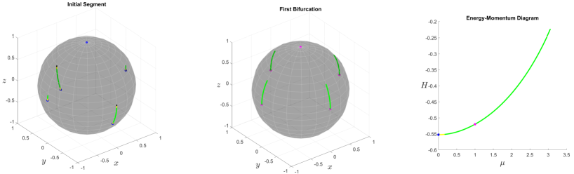
Figure 6.1: CAP of existence and stability of RE for $N=5$ near the ground state. The branch on the leftmost panel is of type $(n_{2},m_{2},p_{1})$ with staggered rings and the branch in the middle is of type $(n_{1},m_{4},p_{0})$.

$N=6$

We establish stability via CAPs of the branch $(n_{2},m_{3},p_{0})$ where the two rings of three vortices are staggered for the values of $0.2\leq\omega\leq 1.4$ which correspond to $0.32\leq\mu\leq 2.36$. We conjecture that this branch (illustrated at equilibrium in Figure 1(f)) is born stable close to the octahedron and is the global minimiser of $H$ for fixed values of $\mu>0$ close to zero. Our analysis shows that this branch loses stability around $\omega=1.4150$ and $\mu=2.38$. We claim that an asymmetric RE gains stability at this point since we do not observe a bifurcation in the map $F$ (3.15) with $m=3$ and no other apparent symmetries are visible. The results are illustrated in Figure 6.2.

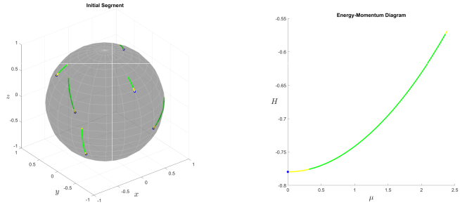
Figure 6.2: CAP of existence and stability of the RE of type $(n_{2},m_{3},p_{0})$ for $N=6$ near the ground state.

$N=7$

In this case Corollary 3.12 may not be used to prove local existence of branches of RE since the non-degeneracy condition is not satisfied. However, a direct calculation shows that the configuration $(n_{1},m_{5},p_{2})$ consisting of 1 ring of 5 vortices arranged at the vertices of a horizontal pentagon at height $z\in(-1,1)$ together with the North and South poles is a RE provided that $\omega=\frac{3z}{1-z^{2}}$. The corresponding value of the momentum is $\mu=5z$ since the contribution from the vortices at the North and South pole vanishes. Note that both the angular velocity $\omega$ and the momentum $\mu$ vanish at the pentagonal bipyramid which is attained when $z=0$.

The stability of these RE can be examined analytically with the approach of section 4. As seen from Table 4.3, the stability is guaranteed by the positive definiteness of the Hermitian matrices $\mathcal{Q}_{1}$ and $\mathcal{Q}_{2}$ which are respectively $3\times 3$ and $2\times 2$. With the help of a symbolic software one finds that they are both real and given by

$$\mathcal{Q}_{1}=\left(\begin{array}[]{ccc}25z^{2}+5&-\frac{5}{2}(z(5z+2)+5)&\frac{5}{2}(z(5z-2)+5)\\ -\frac{5}{2}(z(5z+2)+5)&25(4-3z)z+65&\frac{5}{2}\left(1-5z^{2}\right)\\ \frac{5}{2}(z(5z-2)+5)&\frac{5}{2}\left(1-5z^{2}\right)&65-25z(3z+4)\\ \end{array}\right),\qquad\mathcal{Q}_{2}=\left(\begin{array}[]{cc}15&0\\ 0&15z^{2}\\ \end{array}\right).$$ (6.1)

It is clear that $\mathcal{Q}_{2}$ is positive definite for any value of $z$ different from $0$. On the other hand, we have the following.

Proposition 6.2.

The matrix $\mathcal{Q}_{1}$ in (6.1) is positive definite for $0<|z|<\sqrt{\frac{1}{35}\left(43-4\sqrt{109}\right)}\approx 0.188132$.

Proof.

A direct calculation gives $\det\mathcal{Q}_{1}=\frac{9375}{2}z^{2}\left(35z^{4}-86z^{2}+3\right)$, which shows that $\det\mathcal{Q}_{1}$ can only change sign when $z^{2}=0$ or $z^{2}=\frac{1}{35}\left(43\pm 4\sqrt{109}\right)$. In particular, none of its eigenvalues can vanish for $0<|z|<\sqrt{\frac{1}{35}\left(43-4\sqrt{109}\right)}$. It is then elementary to verify that all 3 eigenvalues are positive for a particular value of $z$ in this interval. ∎

Therefore, we have proved that the branch $(n_{1},m_{5},p_{2})$ (illustrated at equilibrium in Figure 2(b)) arises a stable branch of RE from the pentagonal dypiramid and loses stability at $|z|=\sqrt{\frac{1}{35}\left(43-4\sqrt{109}\right)}$ which corresponds to $|\omega|=\frac{1}{4}\sqrt{89-8\sqrt{109}}$. We conjecture that this branch minimises $H$ for fixed and small values of the momentum. (We mention that these analytic results are in perfect correspondence with the ones predicted by our numerics and CAPs).

Remark 6.3.

Denote by $a$ the equilibrium configuration attained when $z=0$ (the pentagonal bipyramid of Table 1.1). The zero eigenvalue of the matrix $\mathcal{Q}_{2}$ at this point corresponds to a 2-dimensional null space of $d^{2}H(a)$ spanned by the real and imaginary parts of the vector $\hat{C}_{1,2}$. These vectors lie on the space $U_{2}$ of the symplectic slice defined in Lemma 4.6 and are therefore transversal to $\mathfrak{so}(3).a$. This leads to the surprising conclusion that, according to Definition 3.1, the $SO(3)$-orbit of the pentagonal bipyramid is a degenerate critical manifold of $H$ when $N=7$. In particular, it is not possible to determine that this configuration is a local minimum of $H$, nor that it is a stable equilibrium of (2.8), using only information from the second derivatives of $H$. This degenerate situation is reminiscent of the well-known Thomson heptagon problem of stability of a ring of $7$ vortices on the plane (see e.g. [37, 60]).

$N=8$

Using CAPs we establish stability of the branch $(n_{2},m_{4},p_{0})$ emerging from the cubic antiprism for $0.2\leq\omega\leq 1.6$ which corresponds to $0.31\leq\mu\leq 2.6$. We conjecture that this branch (illustrated at equilibrium in Figure 2(d)) is born stable and minimises $H$ for small fixed values of $\mu$. The branch is illustrated in the leftmost panel of Figure 6.3 where one can appreciate that the two rings are staggered.

Our investigations showed that this branch bifurcates into $(n_{4},m_{2},p_{0})$ around $\omega=1.61$ and $\mu=2.61$. We give a CAP of the stability of this new branch on the interval $1.62\leq\omega\leq 1.9$ which corresponds to $2.62\leq\mu\leq 3.05$, and is illustrated in the middle panel of Figure 6.3. This branch loses stability at around $\omega=1.94$ and $\mu=3.12$ and we conjecture that an asymmetric RE gains stability around these values since we do not observe a bifurcation in the corresponding map $F$ (3.15) with $m=2$ and no other apparent symmetries are visible.

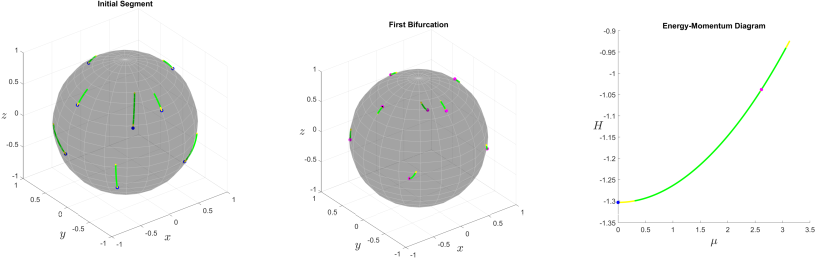
Figure 6.3: CAP of existence and stability of RE for $N=8$ near the ground state. The branch on the leftmost panel is of type $(n_{2},m_{4},p_{0})$ with staggered rings and the branch in the middle is of type $(n_{4},m_{2},p_{0})$.

$N=9$

Our CAP establishes stability of the branch $(n_{3},m_{3},p_{0})$ on the interval $0.3\leq\omega\leq 4.98$ corresponding to $0.45\leq\mu\leq 5.93$ and we conjecture that this branch (illustrated at equilibrium in Figure 2(f)) is born stable and minimises $H$ for fixed small positive values of $\mu$. We found 2 bifurcations that maintain the $(n_{3},m_{3},p_{0})$ symmetry around $\omega=4.99$ and $\omega=5.22$ (which correspond to $\mu=5.94$ and $\mu=6.05$). For these new branches we give CAPs of stability on the intervals $5.03\leq\omega\leq 4.98$, and $5.225\leq\omega\leq 7.53$, which correspond to $5.96\leq\mu\leq 6.03$, and $6.06\leq\mu\leq 6.85$. These results are illustrated in Figure 6.4.

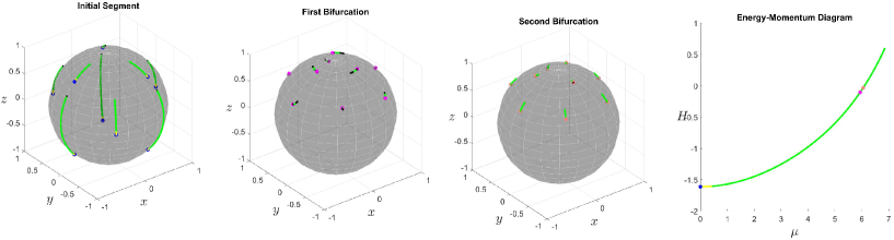
Figure 6.4: CAP of existence and stability of RE for $N=9$ near the ground state. All branches are of type $(n_{3},m_{3},p_{0})$.

$N=10$

Our investigations indicated that the symmetric branches emerging from the equilibrium (i.e. $(n_{2},m_{4},p_{0})$ and $(n_{5},m_{2},p_{0})$ illustrated in Figures 2(h) and 2(g)) fail the stability test of Section 4. Therefore, we conjecture that the stable branch that minimises $H$ for small fixed values of $\mu$ is asymmetric.

We looked for this asymmetric minimising branch numerically and, in view of Remark 3.11, were forced to implement our continuations starting from $\omega$ away from zero. We were only able to produce a CAP of existence of this branch for $1\leq\omega\leq 2.27$ which corresponds to $1.5\leq\mu\leq 3.5$. On the other hand, we give a CAP of stability for the interval $1.56\leq\omega\leq 2.2$, which corresponds to $2.39\leq\mu\leq 3.40$. The branch remains stable until a bifurcation around $\omega=2.29$ and $\mu=3.53$, after which we could not find a stable branch. These results are illustrated in Figure 6.5.

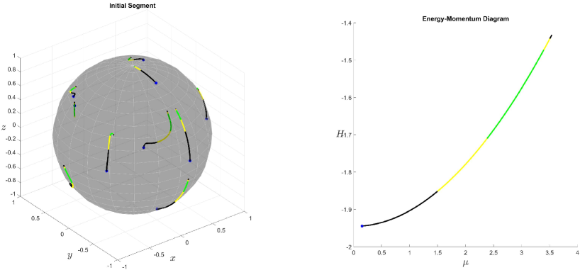
Figure 6.5: CAP of existence and stability of RE for $N=10$ near the ground state. The branch has no symmetry.

$N=11$

We give a CAP of stability of the branch $(n_{5},m_{2},p_{1})$ on the interval $0.5\leq\omega\leq 1.26$ which corresponds to $0.74\leq\mu\leq 1.88$, as illustrated in the left panel of Figure 6.6. We conjecture that this branch (illustrated in Figure 2(i)) is born stable and minimises $H$ for small fixed values of $\mu$. This branch bifurcates and loses stability around $\omega=1.28$ and $\mu=1.90$. We were able to give a CAP of stability of an asymmetric branch in the interval $1.35\leq\omega\leq 1.46$ which corresponds to $2.02\leq\mu\leq 2.19$ (illustrated in the middle panel of Figure 6.6). This branch undergoes another bifurcation around $\omega=1.47$ and $\mu=2.21$ but we were not able to find a stable branch afterwards.

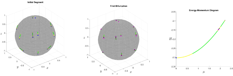
Figure 6.6: CAP of existence and stability of RE for $N=11$ near the ground state. The first branch is $(n_{5},m_{2},p_{1})$ and the second has no symmetries.

$N=12$

We established stability of the branch $(n_{4},m_{3},p_{0})$ with the CAP illustrated in Figure 6.7 on the interval $0.9\leq\omega\leq 2.84$ which corresponds to $1.31\leq\mu\leq 4.26$. We conjecture that this branch (illustrated at equilibrium in Figure 1(i)) is born stable and minimises $H$ for fixed small positive values of $\mu$. This branch loses stability around $\omega=2.85$ and $\mu=4.28$. We claim that an asymmetric RE gains stability around these values since we do not observe a bifurcation in the corresponding map $F$ (3.15) with $m=3$ and no other apparent symmetries are visible.

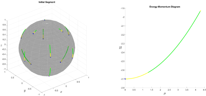
Figure 6.7: CAP of existence and stability of RE for $N=12$ near the ground state. The branch is $(n_{4},m_{3},p_{0})$.

6.3 Stable RE near total collision

We now focus on investigating stable RE near total collision at the North pole. It is easy to see, from the expression of $\Phi$ in (2.9), that this corresponds to $\mu$ approaching the upper bound $N$ of $\Phi$.

The simplest RE of the equations of motion (2.8) is $(n_{1},m_{N},p_{0})$ (consisting of a single horizontal ring where the vortices are located at the vertices of a regular $N$-gon). Such RE is known to be (linearly) unstable if $N\geq 7$ and instead (nonlinearly) stable if $N\leq 6$ and the height $z$ of the ring is sufficiently close to one of the poles (the threshold value of $z$ is given in Table 6.1 below). These conclusions follow from [40, Theorem 5.2] and appear in earlier references [57, 7]. It is reasonable to conjecture that for $N\leq 6$ these RE minimise $H$ for fixed values of $\mu$ sufficiently close to $N$ (i.e. near total collision).

The presence of an additional vortex at the North pole has a stabilising effect. Indeed, as follows from [40, Theorem 6.2] (see also [15]) the RE $(n_{1},m_{N-1},p_{1})$ (consisting of one vortex at the North pole and a regular horizontal $(N-1)$-gon) is stable for $N\leq 9$ provided again that the height $z$ of the ring containing the polygon is sufficiently close to the North pole (the threshold value of $z$ is given in Table 6.1 below). Therefore, it is reasonable to conjecture that for $N=7,8,9$ these RE minimise $H$ for fixed values of $\mu$ sufficiently close to $N$ and this conjecture is supported by numerical experiments.

$N$	$\begin{array}[]{cc}\mbox{Stability region of}\\ \mbox{the RE $(n_{1},m_{N},p_{0})$}\end{array}$	$\begin{array}[]{cc}\mbox{Stability region of}\\ \mbox{the RE $(n_{1},m_{N-1},p_{1})$}\end{array}$
$4$	$|z|>\frac{1}{\sqrt{3}}$	$z>-\frac{1}{3}$
$5$	$|z|>\frac{1}{\sqrt{2}}$	$z>0$
$6$	$|z|>\frac{2}{\sqrt{5}}$	$z>\frac{1}{5}(\sqrt{6}-1)$
$7$	-	$z>\frac{1}{6}(\sqrt{19}-1)$
$8$	-	$z>\frac{5}{7}$
$9$	-	z¿$\frac{1}{8}(\sqrt{65}-1)$

Table 6.1: Stability regions for RE with 1 ring with (right column) and without (left column) a vortex at the North pole. As usual, $N$ is the total number of vortices and all of them have identical strengths.

For $N\geq 10$ both branches $(n_{1},m_{N},p_{0})$ and $(n_{1},m_{N-1},p_{1})$ are always unstable and there is no obvious candidate for the branch of (stable) RE minimising the Hamiltonian $H$ as the momentum $\mu\to N$ (i.e. as the vortices approach total collision). Below we attempt to give a partial answer to this question for $N=10,11,12$. Starting from a numerical approximation of such minimiser for a specific $\mu$ close to $N$, we applied the procedure of section 5 to prove existence and stability of a RE. However, in contrast with the approach followed in section 6.2, due to the large fluctuations of the energy and angular velocity obtained for small configuration variations near total collision, we did not attempt to validate branches of RE but had to settle with the analysis of an isolated one (that we chose to have $\omega=50$). The RE that we found are illustrated in Figure 6.8 and approximated numerically in Appendix E. They all appear to have a central triangle with the remaining vortices organised more or less uniformly in an outer ring. We were only able to make precise symmetry statements for $N=12$.

$N=10$

We proved existence and stability of the RE given in (E.1) for $\omega=50$. The tolerance bound on each coordinate is $4\times 10^{-13}$. This RE is illustrated in Figure 8(a). Although it appears to have some symmetry, we are unable to make any precise statements about it. Note however that there are four pairs of vortices whose heights differ by at most $8\times 10^{-13}$ (i.e. the pairs $(a_{1},a_{6}),(a_{2},a_{4}),(a_{5},a_{10})$ and $(a_{8},a_{9})$ in (E.1)).

$N=11$

For $\omega=50$, we proved the existence of the RE illustrated in Figure 8(b) and whose coordinates are given by (E.2) (with tolerance bound on each coordinate of $6\times 10^{-11}$). As above, we are unable to make any precise statements about the symmetries of this RE. We can only establish that the height of 4 pairs of vortices differs by at most $2\times 10^{-10}$ (i.e. the pairs $(a_{1},a_{10}),(a_{2},a_{8}),(a_{5},a_{7})$ and $(a_{6},a_{11})$ in (E.2)) while the heights of the others are shown to be distinct. For this RE we can only report numerical evidence of stability since our CAP for stability failed due to the clustering of eigenvalues.

$N=12$

This time, for $\omega=50$, we obtained CAPs of the existence and stability of a $\mathbb{Z}_{3}$-symmetric RE of type $(n_{4},m_{3},p_{0})$ whose generators are given by (E.3) (with tolerance bound on each coordinate of $3\times 10^{-13}$). Our proof also shows that the height of two of the four rings (those corresponding to $u_{3}$ and $u_{4}$ in (E.3)) differ by at most $5\times 10^{-13}$. This RE is illustrated in Figure 8(c).

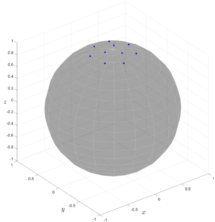
(a) $N=10$

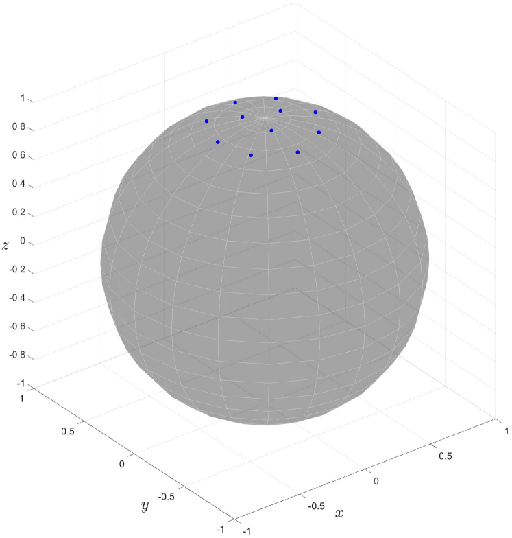
(b) $N=11$

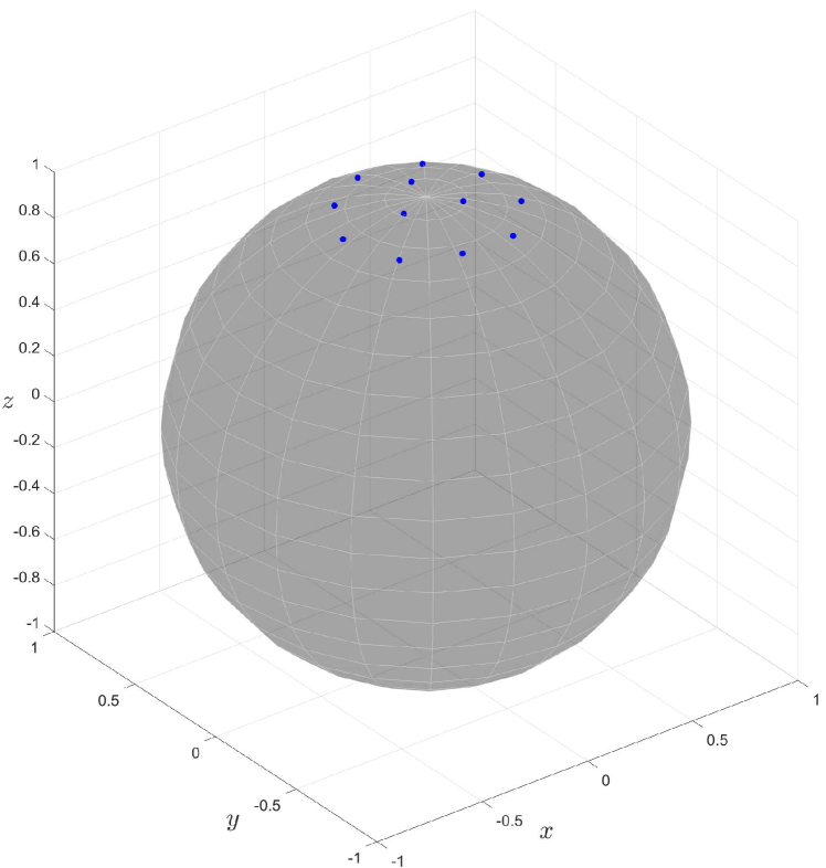
(c) $N=12$

Figure 6.8: Relative equilibria near total collision having $\omega=50$. Their existence is established via CAPs (with tolerance bounds given in the text). On the other hand, their stability has also been demonstrated for $N=10$ and $N=12$ with a CAP whereas for $N=11$ we only have numerical evidence of it.

Statements and declarations

The authors have no competing interests to declare that are relevant to the content of this article.

Data availability statement

The code to reproduce the CAPs presented in our paper is available in [20].

Appendix A Geometric preliminaries

The phase space $M$ of the system is the open subset of $(S^{2})^{N}=S^{2}\times\dots\times S^{2}$ ($N$ copies) obtained by removing the collision configurations. The component $v_{j}$ of the element $v=(v_{1},\dots,v_{N})\in M$ specifies the position of the $j^{th}$ vortex. Throughout the paper we represent $(S^{2})^{N}$ as the embedded submanifold in $(S^{2})^{N}$ specified by $(S^{2})^{N}:=R^{-1}(0)$ where $R:=(R_{1},\dots,R_{N}):(\mathbb{R}^{3})^{N}\to\mathbb{R}^{N}$,

$$R_{j}:(\mathbb{R}^{3})^{N}\to\mathbb{R},\qquad(x_{1},\dots,x_{N})\mapsto\frac{1}{2}(\|x_{j}\|^{2}-1).$$

This embedding induces a convenient identification of tangent vectors to $M$ with vectors in $\mathbb{R}^{3N}$. Specifically, if $v=(v_{1},\dots,v_{N})\in M$ we identify

$$T_{v}M=V_{v}:=\{\,{\bf w}=(w_{1},\dots,w_{N})\in(\mathbb{R}^{3})^{N}\,:\,v_{j}\cdot w_{j}=0\,\},$$

where $\cdot$ is the euclidean scalar product in $\mathbb{R}^{3}$.

Let $f:M\to\mathbb{R}$. The differential of $f$ at $v\in M$ is the linear map $df(v):V_{v}\to\mathbb{R}$ defined intrinsically by

$$df(v)({\bf w})=L_{X}f(v),\qquad{\bf w}\in V_{v},$$

where $X$ is any locally defined vector field on $M$ satisfying $X(v)={\bf w}$ and $L_{X}$ denotes the Lie derivative along $X$. Note that $df(v)\in V_{v}^{*}$. If $\tilde{f}:(\mathbb{R}^{3})^{N}\to\mathbb{R}$ is any smooth extension of $f$, then

$$df(v)({\bf w})=\langle\nabla_{x}\tilde{f}(v),{\bf w}\rangle,$$

where $\langle\cdot,\cdot\rangle$ is the euclidean inner product in $(\mathbb{R}^{3})^{N}$ and $\nabla_{x}\tilde{f}(v)$ is the standard gradient of $\tilde{f}$ evaluated at $v\in(\mathbb{R}^{3})^{N}$.

A point $a\in M$ is a critical point of $f$ if $df(a)=0$. Hence, $a$ is a critical point of $f$ if and only if for any smooth extension $\tilde{f}:(\mathbb{R}^{3})^{N}\to\mathbb{R}$ of $f$ one has

$$\langle\nabla_{x}\tilde{f}(a),{\bf w}\rangle=0\qquad\forall{\bf w}\in V_{a}.$$

In other words, $\nabla_{x}\tilde{f}(a)\in V_{a}^{\perp}$. Considering that $V_{a}^{\perp}=\mathrm{span}\{\nabla_{x}R_{i}(a)\,:\,i=1,\dots,N\}$, we conclude that if $a\in M$ is a critical point of $f$ and $\tilde{f}$ is an extension then:

1. There exist Lagrange multipliers $c_{1},\dots,c_{N}\in\mathbb{R}$ such that

   $$\nabla_{x}\tilde{f}(a)+\sum_{i=1}^{N}c_{i}\nabla_{x}R_{i}(a)=0.$$

2. Define the function $\tilde{f}^{*}:(\mathbb{R}^{3})^{N}\times\mathbb{R}^{N}\to\mathbb{R}$ by

   $$\tilde{f}^{*}\left(x,\lambda\right):=\tilde{f}(x)+\sum_{i=1}^{N}\lambda_{i}R_{i}(x),\qquad x=(x_{1},\dots,x_{N})\in(\mathbb{R}^{3})^{N},\;\lambda=(\lambda_{1},\dots,\lambda_{N})\in\mathbb{R}^{N}.$$

   Then $\tilde{f}^{*}$ has a critical point at $(a,c)$, with $c=(c_{1},\dots,c_{N})$.

Continue to assume that $a\in M$ is a critical point of $f:M\to\mathbb{R}$. The second derivative of $f$ at $a$ is the symmetric bilinear form $d^{2}f(a):V_{a}\times V_{a}\to\mathbb{R}$ defined intrinsically by

$$d^{2}f(a)({\bf w}_{1},{\bf w}_{2})=L_{X_{1}}L_{X_{2}}f(a)=L_{X_{2}}L_{X_{1}}f(a),$$

where $X_{1}$ and $X_{2}$ are any locally defined vector fields on $M$ satisfying $X_{1}(a)={\bf w}_{1}$, $X_{2}(a)={\bf w}_{2}$. With the definitions introduced above we have

$$d^{2}f(a)({\bf w}_{1},{\bf w}_{2})={\bf w}_{1}^{T}\nabla^{2}_{x}\tilde{f}^{*}(a,c){\bf w}_{2},\qquad\forall{\bf w}_{1},{\bf w}_{2}\in V_{a},$$

where $\nabla^{2}_{x}\tilde{f}^{*}(a,c)$ denotes the standard Hessian matrix of $x\mapsto\tilde{f}^{*}(x,c)$ evaluated at $x=a$.

Appendix B Computation of the gradient and Hessian matrix of the reduced Hamiltonian

Below we give explicit expressions for the gradient and Hessian matrix of the reduced Hamiltonian $h$ given by (3.4) interpreted as function $h:\mathbb{R}^{3n}\to\mathbb{R}$. Throughout this appendix we simplify the notation and write $g:=g_{m}\in SO(3)$ and denote by $I$ the $3\times 3$ identity matrix.

B.1 Gradient $\nabla_{u}h(u)$.

The gradient of the reduced Hamiltonian $h$ has components

$$\nabla_{u_{j}}h(u)=-m\sum_{i=1}^{m-1}\frac{u_{j}-g^{i}u_{j}}{\left\|u_{j}-g^{i}u_{j}\right\|^{2}}-m\sum_{j^{\prime}=1(j^{\prime}\neq j)}^{n}\sum_{i=1}^{m}\frac{u_{j}-g^{i}u_{j^{\prime}}}{\left\|u_{j}-g^{i}u_{j^{\prime}}\right\|^{2}}-m\sum_{f\in F}\frac{u_{j}-f}{\left\|u_{j}-f\right\|^{2}}.$$ (B.1)

To see this, write $M:=I-g^{i}$ and compute:

$$\nabla_{u}\ln\left\|Mu\right\|^{2}=\frac{1}{\left\|Mu\right\|^{2}}\nabla_{u}\left\langle Mu,Mu\right\rangle=\frac{1}{\left\|Mu\right\|^{2}}\nabla_{u}\left\langle M^{T}Mu,u\right\rangle=\frac{1}{\left\|Mu\right\|^{2}}\left(2M^{T}M\right)u.$$

Since $M^{T}M=(I-g^{-i})+(I-g^{i})$, we conclude

$$\nabla_{u_{j}}\sum_{i=1}^{m-1}\ln\left\|u_{j}-g^{i}u_{j}\right\|^{2}=2\sum_{i=1}^{m-1}\frac{(I-g^{-i})u+(I-g^{i})u}{\left\|\left(I-g^{i}\right)u\right\|^{2}}=4\sum_{i=1}^{m-1}\frac{(I-g^{i})u}{\left\|\left(I-g^{i}\right)u\right\|^{2}}.$$

Combining these identities with (3.4) proves (B.1).

B.2 Hessian matrix $\nabla^{2}h(u)$.

We now describe the Hessian matrix $\nabla_{u}^{2}h(u)$ in terms of the $3\times 3$ blocks $D_{u_{j^{\prime}}}\nabla_{u_{j}}h(u)$, for the indices $j,j^{\prime}\in\{1,\dots,n\}$.

Case $j^{\prime}\neq j$.

In this case we have:

$$D_{u_{j^{\prime}}}\nabla_{u_{j}}h(u)=m\sum_{i=1}^{m}\frac{1}{\left\|u_{j}-g^{i}u_{j^{\prime}}\right\|^{4}}\left(g^{i}\left\|u_{j}-g^{i}u_{j^{\prime}}\right\|^{2}-2\left(u_{j}-g^{i}u_{j^{\prime}}\right)\left(u_{j}-g^{i}u_{j^{\prime}}\right)^{T}g^{i}\right).$$ (B.2)

To prove (B.2), start with (B.1) and use the condition $j^{\prime}\neq j$ to obtain

$$\begin{split}D_{u_{j^{\prime}}}\nabla_{u_{j}}h(u)&=m\sum_{i=1}^{m}g^{i}D_{u_{j^{\prime}}}\frac{u_{j^{\prime}}-g^{-i}u_{j}}{\left\|u_{j^{\prime}}-g^{-i}u_{j}\right\|^{2}}=m\sum_{i=1}^{m}g^{-i}D_{u_{j^{\prime}}}\frac{u_{j^{\prime}}-g^{i}u_{j}}{\left\|u_{j^{\prime}}-g^{i}u_{j}\right\|^{2}}\\ &=m\sum_{i=1}^{m}g^{-i}\left(\frac{I}{\left\|u_{j^{\prime}}-g^{i}u_{j}\right\|^{2}}-\left\|u_{j^{\prime}}-g^{i}u_{j}\right\|^{-4}\left(u_{j^{\prime}}-g^{i}u_{j}\right)\left(D_{u_{j^{\prime}}}\left\|u_{j^{\prime}}-g^{i}u_{j}\right\|^{2}\right)\right).\end{split}$$

Since $D_{u_{j^{\prime}}}\left\|u_{j^{\prime}}-g^{i}u_{j}\right\|^{2}=2\left(u_{j^{\prime}}-g^{i}u_{j}\right)^{T}$, we may rewrite the above expression as

$$D_{u_{j^{\prime}}}\nabla_{u_{j}}h(u) = m\sum_{i=1}^{m}g^{-i}\frac{1}{\left\|u_{j^{\prime}}-g^{i}u_{j}\right\|^{4}}\left(I\left\|u_{j^{\prime}}-g^{i}u_{j}\right\|^{2}-2\left(u_{j^{\prime}}-g^{i}u_{j}\right)\left(u_{j^{\prime}}-g^{i}u_{j}\right)^{T}\right),$$

$$= m\sum_{i=1}^{m}g^{i}\frac{1}{\left\|u_{j}-g^{i}u_{j^{\prime}}\right\|^{4}}\left(I\left\|u_{j}-g^{i}u_{j^{\prime}}\right\|^{2}-2\left(u_{j^{\prime}}-g^{-i}u_{j}\right)\left(u_{j^{\prime}}-g^{-i}u_{j}\right)^{T}\right),$$

$$= m\sum_{i=1}^{m}g^{i}\frac{1}{\left\|u_{j}-g^{i}u_{j^{\prime}}\right\|^{4}}\left(I\left\|u_{j}-g^{i}u_{j^{\prime}}\right\|^{2}-2g^{-i}\left(g^{i}u_{j^{\prime}}-u_{j}\right)\left(g^{i}u_{j^{\prime}}-u_{j}\right)^{T}g^{i}\right),$$

which simplifies to (B.2).

Case $j^{\prime}=j$.

In this case we have:

$$D_{u_{j}}\nabla_{u_{j}}h(u)=\mathcal{A}_{1}(u)+\mathcal{A}_{2}(u)+\mathcal{A}_{3}(u),$$

where the $3\times 3$ matrices $\mathcal{A}_{j}(u)$ arise from the differentiation of the three terms in (B.1). We prove below that these are given by

$$\mathcal{A}_{1}(u)=-m\sum_{i=1}^{m-1}\left(\frac{(I-g^{i})}{\left\|u_{j}-g^{i}u_{j}\right\|^{2}}+\frac{2}{\left\|u_{j}-g^{i}u_{j}\right\|^{4}}\left(u_{j}-g^{i}u_{j}\right)\left(u_{j}-g^{i}u_{j}\right)^{T}(I-g^{i})\right),$$ (B.3)

$$\mathcal{A}_{2}(u)=-m\sum_{j^{\prime}=1(j^{\prime}\neq j)}^{n}\sum_{i=1}^{m}\left(\frac{I}{\left\|u_{j}-g^{i}u_{j^{\prime}}\right\|^{2}}-\frac{2}{\left\|u_{j}-g^{i}u_{j^{\prime}}\right\|^{4}}\left(u_{j}-g^{i}u_{j^{\prime}}\right)\left(u_{j}-g^{i}u_{j^{\prime}}\right)^{T}\right),$$ (B.4)

$$\mathcal{A}_{3}(u)=-m\sum_{f\in F}\left(\frac{I}{\left\|u_{j}-f\right\|^{2}}-\frac{2}{\left\|u_{j}-f\right\|^{4}}\left(u_{j}-f\right)\left(u_{j}-f\right)^{T}\right).$$ (B.5)

The validity of (B.4) and (B.5) follows from the identities

$$\begin{split}D_{u_{j}}\frac{u_{j}-g^{i}u_{j^{\prime}}}{\left\|u_{j}-g^{i}u_{j^{\prime}}\right\|^{2}}&=\frac{I}{\left\|u_{j}-g^{i}u_{j^{\prime}}\right\|^{2}}-\frac{2}{\left\|u_{j}-g^{i}u_{j^{\prime}}\right\|^{4}}\left(u_{j}-g^{i}u_{j^{\prime}}\right)\left(u_{j}-g^{i}u_{j^{\prime}}\right)^{T},\\ D_{u_{j}}\frac{u_{j}-f}{\left\|u_{j}-f\right\|^{2}}&=\frac{I}{\left\|u_{j}-f\right\|^{2}}-\frac{2}{\left\|u_{j}-f\right\|^{4}}\left(u_{j}-f\right)\left(u_{j}-f\right)^{T},\end{split}$$

which are deduced proceeding as above. For (B.3), we write $M=I-g^{i}$ as before and write

$$D_{u_{j}}\frac{u_{j}-g^{i}u_{j}}{\left\|u_{j}-g^{i}u_{j}\right\|^{2}}=D_{u_{j}}\frac{Mu_{j}}{\left\|Mu_{j}\right\|^{2}}=\frac{M}{\left\|Mu_{j}\right\|^{2}}+Mu_{j}D_{u_{j}}\left(\left\|Mu_{j}\right\|^{2}\right)^{-1}.$$

We have that $D_{u_{j}}\left(\left\|Mu_{j}\right\|^{2}\right)^{-1}=\left(\left\|Mu_{j}\right\|^{2}\right)^{-2}D_{u_{j}}\left\|Mu_{j}\right\|^{2}$ and using the computation of $D_{u_{j}}\left\|Mu_{j}\right\|^{2}$ as before we obtain

$$D_{u_{j}}\frac{u_{j}-g^{i}u_{j}}{\left\|u_{j}-g^{i}u_{j}\right\|^{2}}=\frac{M}{\left\|Mu_{j}\right\|^{2}}+\frac{2}{\left\|Mu_{j}\right\|^{4}}Mu_{j}\left(Mu_{j}\right)^{T}M.$$

Therefore,

$$D_{u_{j}}\frac{u_{j}-g^{i}u_{j}}{\left\|u_{j}-g^{i}u_{j}\right\|^{2}}=\frac{I-g^{i}}{\left\|u_{j}-g^{i}u_{j}\right\|^{2}}+\frac{2}{\left\|u_{j}-g^{i}u_{j}\right\|^{4}}\left(u_{j}-g^{i}u_{j}\right)\left(u_{j}-g^{i}u_{j}\right)^{T}(I-g^{i}),$$

proving the validity of (B.3).

Appendix C General non-symmetric symplectic slice

Here we construct a symplectic slice for a RE $(a,\omega)\in M\times\mathbb{R}$ which does not assume any symmetry. We assume that both $\mu=\Phi(a)$ and $\omega$ are non-zero and that all vortices have equal strengths and $N\geq 3$. Write $a=(a_{1},\dots,a_{N})\in M$ and suppose that the arrangement of the vortices is such that $a_{1}$ and $a_{2}$ do not have equal nor opposite latitudes, and are not poles (otherwise do a suitable permutation). We work with the identification $T_{a}M=V_{a}$ given by (4.1).

Define the vectors $b_{j},c_{j}\in\mathbb{R}^{3}$, $j=1,\dots,N$, as follows:

$$\begin{split}b_{j}:=\begin{cases}e_{3}\times a_{j}\quad\mbox{if $a_{j}$ is not a pole,}\\ e_{1}\qquad\mbox{if $a_{j}$ is a pole,}\end{cases}\qquad c_{j}:=a_{j}\times b_{j}.\end{split}$$

Proposition C.1.

Under the condition that $a_{1}$ and $a_{2}$ do not have equal nor opposite latitudes, and are not poles, the set $\{{\bf u}^{(j)},{\bf v}^{(j)}\}_{j=1}^{N-1}$, whose elements are defined below, forms a basis of a symplectic slice.

$$\begin{split}{\bf u}^{(1)}&=\left(a_{1}\times(b_{2}\times c_{2}),-a_{1}\times(b_{2}\times c_{2}),0,\dots,0\right),\\ {\bf u}^{(j)}&=\left(a_{1}\times(b_{2}\times b_{j+2}),-(a_{1}\cdot b_{j+2})b_{2},0,\dots,0,\stackrel{{\scriptstyle(j+2)^{th}}}{{(a_{1}\cdot b_{2})b_{j+2}}},0,\dots,0\right),\quad j=2,\dots,N-2,\\ {\bf v}^{(j)}&=\left(a_{1}\times(b_{2}\times c_{j+2}),-(a_{1}\cdot c_{j+2})b_{2},0,\dots,0,\stackrel{{\scriptstyle(j+2)^{th}}}{{(a_{1}\cdot b_{2})c_{j+2}}},0,\dots,0\right),\quad j=1,\dots,N-2.\end{split}$$ (C.1)

Proof.

First note that the condition that $a_{1}$ and $a_{2}$ do not have opposite latitudes, and are not poles guarantees that the scalar product $a_{1}\cdot b_{2}\neq 0$. Consider the following $2(N-2)+1$ vectors in $(\mathbb{R}^{3})^{N}$

$$\begin{split}\boldsymbol{\gamma}&=\left(a_{1}\times(b_{2}\times c_{2}),-a_{1}\times(b_{2}\times c_{2}),0,\dots,0\right),\\ \alpha^{(j)}&=\left(a_{1}\times(b_{2}\times b_{j+2}),-(a_{1}\cdot b_{j+2})b_{2},0,\dots,0,\stackrel{{\scriptstyle(j+2)^{th}}}{{(a_{1}\cdot b_{2})b_{j+2}}},0,\dots,0\right),\quad j=1,\dots,N-2,\\ \beta^{(j)}&=\left(a_{1}\times(b_{2}\times c_{j+2}),-(a_{1}\cdot c_{j+2})b_{2},0,\dots,0,\stackrel{{\scriptstyle(j+2)^{th}}}{{(a_{1}\cdot b_{2})c_{j+2}}},0,\dots,0\right),\quad j=1,\dots,N-2.\end{split}$$

Using that $\{a_{j},b_{j},c_{j}\}$ is an orthogonal basis of $\mathbb{R}^{3}$ for all $j=1,\dots,N$, one proves that the above vectors belong to $V_{a}$ defined by (4.1). Moreover, a straightforward calculation using (4.12), shows that these vectors actually belong to $\ker d\Phi(a)$. We wish to show that they form a basis for $\ker d\Phi(a)$. Considering that the dimension of $\ker d\Phi(a)$ is $2N-3$ then it suffices to prove their linear independence. Take a linear combination of them equal to zero:

$$\lambda_{0}\gamma+\sum_{k=1}^{N-2}(\lambda_{k}\alpha^{(k)}+\mu_{k}\beta^{(k)})=0.$$

For $1\leq j\leq N-2$ the $(j+2)^{th}$ entry of the above vector is $(a_{1}\cdot b_{2})(\lambda_{j}b_{j+2}+\mu_{j}c_{j+2})$. Given that $a_{1}\cdot b_{2}\neq 0$ and considering that $b_{j}$ and $c_{j}$ are perpendicular, this vector can only equal zero if $\lambda_{j}=\mu_{j}=0$. Therefore we are left with $\lambda_{0}\gamma=0$ which leads to $\lambda_{0}=0$, proving our claim.

Now we claim that the infinitesimal generator of the orbit, $s_{a}$, is a linear combination of the vectors $\alpha^{(k)}$, $k=1,\dots,N-2$. To see this, first assume that there are no poles so that

$$b_{j}=J_{3}a_{j}=e_{3}\times a_{j},\quad\mbox{for all}\quad 1\leq j\leq N,\qquad s_{a}=(b_{1},\dots,b_{N}).$$

On the other hand we have

$$\frac{1}{a_{1}\cdot b_{2}}\sum_{j=1}^{N}\alpha^{(j)}=\left(\frac{1}{a_{1}\cdot b_{2}}a_{1}\times\left(b_{2}\times\sum_{j=3}^{N}b_{j}\right),-\frac{a_{1}\cdot\left(\sum_{j=3}^{N}b_{j}\right)}{a_{1}\cdot b_{2}}\,b_{2},b_{3},\dots,b_{N}\right).$$

Now note that by Proposition 2.3(ii) we have $\sum_{j=1}^{N}b_{j}=e_{3}\times\sum_{j=1}^{N}a_{j}=e_{3}\times\Phi(a)=0$, so we may write

$$\begin{split}\frac{1}{a_{1}\cdot b_{2}}a_{1}\times\left(b_{2}\times\sum_{j=3}^{N}b_{j}\right)&=\frac{1}{a_{1}\cdot b_{2}}a_{1}\times\left(b_{2}\times(-b_{1}-b_{2})\right)\\ &=\frac{-1}{a_{1}\cdot b_{2}}a_{1}\times\left(b_{2}\times b_{1}\right)=b_{1},\end{split}$$

and also

$$-\frac{a_{1}\cdot\left(\sum_{j=3}^{N}b_{j}\right)}{a_{1}\cdot b_{2}}=\frac{a_{1}\cdot b_{1}+a_{1}\cdot b_{2}}{a_{1}\cdot b_{2}}=1.$$

Therefore

$$\frac{1}{a_{1}\cdot b_{2}}\sum_{j=1}^{N}\alpha^{(j)}=s_{a},$$

and $s_{a}$ is indeed a linear combination of the vectors $\alpha^{(k)}$, $k=1,\dots,N-2$.

In the presence of $p$ poles ($p=1,2$), the above calculation gets modified and one instead shows that

$$\frac{1}{a_{1}\cdot b_{2}}\sum_{j=1}^{N-p}\alpha^{(j)}=s_{a},$$

using that $\sum_{j=1}^{N-p}b_{j}=0$. (We use the convention that the poles are at the end of the array $(a_{1},\dots,a_{N})$).

Considering that $s_{a}$ is a linear combination of $\alpha^{(j)}$, $j=1,\dots,N-2$ and that the vectors $\{\gamma,\alpha^{(j)},\beta^{(j)}\}$ are a basis of $\ker d\Phi(a)$ we conclude that the subspace $\mathcal{N}_{a}$ generated by:

$$\gamma,\quad\alpha^{(j)},\,j=2,\dots,N-2,\quad\beta^{(j)},\,j=1,\dots,N-2,$$

is a $2(N-2)$-dimensional subspace of $V_{a}$ which contains $\ker d\Phi(a)$ and is transversal to $s_{a}$ and may therefore be taken as a symplectic slice. The vectors ${\bf u}^{(j)}$, ${\bf v}^{(j)}$ in the statement of the proposition are precisely taken as:

$$\begin{split}{\bf u}^{(1)}=\gamma,\qquad{\bf u}^{(j)}=\alpha^{(j)},\,j=2,\dots,N-2,\qquad{\bf v}^{(j)}=\beta^{(j)},\,j=1,\dots,N-2.\end{split}$$

∎

Appendix D Proof of Lemma 4.9

Proof.

It is obvious that $\mathcal{Q}$ is Hermitian from its definition and in view of (4.32). To prove the statement about the indices of inertia and the dimension of the null spaces let $\{e_{1},\dots,e_{d}\}$ be the canonical basis of $\mathbb{C}^{d}$ and consider $\psi:V\to\mathbb{C}^{d}$ defined by $\psi(\alpha_{j}):=e_{j}$, $\psi(\beta_{j}):=-ie_{j}$, $j=1\dots,d$. Then $\psi$ is a vector space isomorphism between $V$ and $\mathbb{C}^{d}_{\mathbb{R}}$, where $\mathbb{C}^{d}_{\mathbb{R}}$ denotes the set $\mathbb{C}^{d}$ endowed with the vector space structure over $\mathbb{R}$. Let $\tilde{f}:\mathbb{C}^{d}\times\mathbb{C}^{d}\to\mathbb{C}$ be the Hermitian form whose matrix wrt the canonical basis of $\mathbb{C}^{d}$ is $\mathcal{Q}$, namely

$$\tilde{f}(z_{1},z_{2})=\bar{z}_{1}^{T}\mathcal{Q}z_{2},\qquad z_{1},z_{2}\in\mathbb{C}^{d}.$$

The key point of the proof is to notice that

$$f(w_{1},w_{2})=\frac{1}{2}\mbox{Re}\left(\tilde{f}(\psi(w_{1}),\psi(w_{2}))\right),\quad\mbox{for all $w_{1},w_{2}\in V$.}$$ (D.1)

This is a consequence of linearity of $f$, sesquilinearity of $\tilde{f}$, and the identities

$$f(\alpha_{j},\alpha_{k})=f(\beta_{j},\beta_{k})=\frac{1}{2}\mbox{Re}\left(\mathcal{Q}_{jk}\right),\qquad f(\alpha_{j},\beta_{k})=-f(\alpha_{k},\beta_{j})=\frac{1}{2}\mbox{Im}\left(\mathcal{Q}_{jk}\right),$$

which hold $\forall j,k=1,\dots,d$, because of the hypothesis (4.32). In particular we have

$$f(w,w)=\frac{1}{2}\tilde{f}(\psi(w),\psi(w)),\quad\mbox{for all $w\in V$.}$$ (D.2)

Now let $\{s_{1},\dots,s_{d}\}$ be a basis of $\mathbb{C}^{d}$ which diagonalises $\tilde{f}$, i.e. $\tilde{f}(s_{i},s_{j})=0$ if $i\neq j$, and suppose that

$$\begin{split}&\tilde{f}(s_{j},s_{j})>0,\quad 1\leq j\leq d_{+},\qquad\tilde{f}(s_{j},s_{j})<0,\quad d_{+}+1\leq j\leq d_{+}+d_{-},\\ &\tilde{f}(s_{j},s_{j})=0,\quad d_{+}+d_{-}+1\leq j\leq d_{+}+d_{-}+d_{0},\end{split}$$ (D.3)

so that $i_{+}(\tilde{f})=d_{+}$, $i_{-}(\tilde{f})=d_{-}$, $\dim\ker\tilde{f}=d_{0}$, and $d=d_{+}+d_{-}+d_{0}$. Then $\{s_{1},,\dots,s_{d},is_{1},\dots,is_{d}\}$ is a basis of $\mathbb{C}^{d}_{\mathbb{R}}$ and, since $\psi$ is an isomorphism, $\{y_{1},\dots,y_{2d}\}$ defined by

$$y_{j}:=\psi^{-1}(s_{j}),\quad y_{m+j}:=\psi^{-1}(is_{j}),\qquad 1\leq j\leq d,$$

is a basis of $V$. Moreover, since $\{s_{1},\dots,s_{m}\}$ diagonalises $\tilde{f}$, it is easy to show, using (D.1), that $\{y_{1},\dots,y_{2m}\}$ diagonalises $f$, i.e. $f(y_{i},y_{j})=0$ for all $i\neq j$. Using (D.2) and sesquilinearity of $\tilde{f}$ it follows that

$$f(y_{j},y_{j})=f(y_{m+j},y_{m+j})=\frac{1}{2}\tilde{f}(s_{j},s_{j}),\qquad j=1,\dots,m,$$

which by (D.3) imply $i_{+}(f)=2d_{+}$, $i_{-}(f)=2d_{-}$ and $\dim\ker f=2d_{0}$. ∎

Appendix E Approximate coordinates of RE near total collision

An approximation of the coordinates of the RE near total collision reported in section 6.3 is as follows. For all of them $\omega=50$.

For $N=10$ one has

$$\begin{split}a_{1}&=(-0.321250364476975,0.125503906002515,0.938641024514443),\\ a_{2}&=(-0.281614324121647,-0.177060196674640,0.943049871005264),\\ a_{3}&=(-0.110832315744048,0.301948550025117,0.946859689143297),\\ a_{4}&=(0.329289157466230,0.047176175895631,0.943049871005264),\\ a_{5}&=(-0.056029765308738,-0.338564275556233,0.939273600564037),\\ a_{6}&=(0.163769131776852,0.303533686063892,0.938641024514443),\\ a_{7}&=(0.055171327848398,-0.150307266747506,0.987098703345485),\\ a_{8}&=(0.093915265535320,0.096705006907256,0.990872375504786),\\ a_{9}&=(-0.134176736522985,0.012982250865822,0.990872375504786),\\ a_{10}&=(0.261758623547594,-0.221917836781855,0.939273600564037).\end{split}$$ (E.1)

For $N=11$,

$$\begin{split}a_{1}&=(0.139326894549961,0.025868279023347,0.989908505163702),\\ a_{2}&=(-0.023823734155396,-0.359048230308640,0.933014896988857),\\ a_{3}&=(-0.233002228449082,0.278282639870440,0.931809387098295),\\ a_{4}&=(0.216459904805164,-0.258525569202590,0.941440194425656),\\ a_{5}&=(0.034791923532369,0.340414859454908,0.939631441321124),\\ a_{6}&=(-0.275029387518199,-0.219648813034752,0.936009206650121),\\ a_{7}&=(-0.341231039929540,0.025576001826382,0.939631441321107),\\ a_{8}&=(0.357646782971700,-0.039648210890842,0.933014896988869),\\ a_{9}&=(-0.089752690493977,0.107194750077486,0.990178640501257),\\ a_{10}&=(-0.049951742661942,-0.132612121654087,0.989908505163703),\\ a_{11}&=(0.264565317348943,0.232146414838348,0.936009206650103).\end{split}$$ (E.2)

Finally, for $N=12$, the generators of the $\mathbb{Z}_{3}$-symmetric RE of type $(n_{4},m_{3},p_{0})$ are

$$\begin{split}u_{1}&=(0.034887632581048,0.136341626351998,0.990047379682701),\\ u_{2}&=(-0.249324115175042,0.243756694911171,0.937240715759919),\\ u_{3}&=(0.214399606524508,0.302490526779084,0.928726165202127),\\ u_{4}&=(-0.042756936922558,0.368292756396255,0.928726165202127).\end{split}$$ (E.3)

References

- [1] Aref, H., Newton, P. K., Stremler, M. A., Tokieda, T. and D. L. Vainchtein, Vortex crystals. Adv. Appl. Mech. 39 (2003) 1–79.
- [2] Aref, H.: Point vortex dynamics: a classical mathematics playground.J. Math. Phys. 48 (2007) 065401
- [3] Armentano D. Beltrán C. and M. Shub Minimizing the discrete logarithmic energy on the sphere: the role of random polynomials. Trans. Amer. Math. Soc. 363 (2011), 2955–2965.
- [4] Beltrán Álvarez, C. On Smale’s 7th problem. (Spanish) Gac. R. Soc. Mat. Esp. 23 (2020), 507–534.
- [5] van den Berg, J. B. and J. P. Lessard, Rigorous numerics in dynamics. Notices Amer. Math. Soc., 62 (2015) 1057–1061.
- [6] van den Berg, J. B. and J. P. Lessard, editors. Rigorous numerics in dynamics, volume 74 of Proceedings of Symposia in Applied Mathematics. American Mathematical Society, Providence, RI, (2018). AMS Short Course: Rigorous Numerics in Dynamics, January 4–5, 2016, Seattle, Washington.
- [7] S. Boatto and H. E. Cabral, Nonlinear stability of a latitudinal ring of point-vortices on a non rotating sphere SIAM J. Appl. Math. 64 (2003) 216–230.
- [8] Boatto S. and J. Koiller. Vortices on Closed Surfaces. Geometry, Mechanics, and Dynamics. Fields Institute Communications, 73 (2015) 185–237.
- [9] Bogomolov, V. A., Dynamics of vorticity at a sphere. Fluid. Dyn. (USSR) 6, (1977) 863–870.
- [10] Borisov, A. V. and Lebedev, V. G., Dynamics of three vortices on a plane and a sphere II. Regul. Chaotic Dyn. 3, 99–114 (1998).
- [11] Borisov, A. V. and Pavlov, A. E., Dynamics and statics of vortices on a plane and a sphere I. Regul. Chaotic Dyn. 3, 28–38 (1988).
- [12] Borisov, A. V., Kilin, A. A. and I. S. Mamaev, A New Integrable Problem of Motion of Point Vortices on The Sphere. In: Borisov, A.V., Kozlov, V.V., Mamaev, I.S., Sokolovskiy, M.A. (eds)IUTAM Symposium on Hamiltonian Dynamics, Vortex Structures, Turbulence. IUTAM Bookseries, vol 6. Springer, Dordrecht. (2008).
- [13] Borisov, A. V. and A. A. Kilin, Stability of Thomson’s configurations of vortices on a sphere, Regul. Chaotic Dyn., 5 (2000) 189–200.
- [14] Bott, R. Nondegenerate critical manifolds. Ann. Math. 60 (1954), 248–261.
- [15] Cabral, H. E., Meyer K. R. and D. S. Schmidt, Stability and bifurcations for the vortex problem on the sphere. Regul. Chaotic Dyn.8 (2003), 259–282.
- [16] Calleja, R. C., Doedel, E. J. and C. García-Azpeitia, Choreographies in the -vortex Problem. Regul. Chaot. Dyn. 23 (2018) 595–612.
- [17] Chow S. N. and J. K. Hale, Methods of bifurcation theory, volume 251 of Grundlehren der Mathematischen Wissenschaften [Fundamental Principles of Mathematical Science]. Springer-Verlag, New York, 1982.
- [18] Church, K. E. M. and J. P. Lessard, Rigorous verification of Hopf bifurcations in functional differential equations of mixed type. Phys. D, 429 (2022) 133072.
- [19] Constantineau, K, García-Azpeitia, C. and J. P. Lessard. Spatial relative equilibria and periodic solutions of the Coulomb -body problem. Qual. Theory Dyn. Syst., 21 (2022).
- [20] Constantineau, K., Support code for “Determination of stable branches of relative equilibria of the -vortex problem on the sphere”, https://github.com/BaronNashville/vortices_code.
- [21] Doedel, E. J., Lecture notes on numerical analysis of nonlinear equations. In Numerical continuation methods for dynamical systems, Underst. Complex Syst., pages 1–49. Springer, Dordrecht, 2007.
- [22] Dragnev, P. D., Legg, D. A. and D.W. Townsend, Discrete logarithmic energy on the sphere. Pacific J. Math. 207 (2002), 345–358.
- [23] Fontaine, M. and J. Montaldi, Persistence of stationary motion under explicit symmetry breaking perturbation, Nonlinearity 32 (6), (2019).
- [24] García-Azpeitia, C., Relative periodic solutions of the -vortex problem on the sphere. J. Geom. Mech. 11 (2019) 427–438.
- [25] García-Azpeitia, C. and L. C. García-Naranjo. Platonic solids and dynamics of symmetric configurations for vortices on the sphere. J Nonlinear Sci 32 (2022).
- [26] Gómez-Serrano, J. Computer-assisted proofs in PDE: a survey. SeMA, 76 (2019) 459–484.
- [27] Gromeka, L. S., On vortex motions of liquid on a sphere, Collected Papers Moscow, AN USSR, 296, (1952).
- [28] Hansen, E. R. and R. I. Greenberg, An interval Newton method. Appl. Math. Comput., 12 (1983) 89–98.
- [29] Ize, J. and A. Vignoli. Equivariant degree theory. De Gruyter Series in Nonlinear Analysis and Applications 8. Walter de Gruyter, Berlin, 2003.
- [30] Kapela, T., Mrozek, M., Wilczak, D. and P. Zgliczyński. CAPD::DynSys: a flexible C++ toolbox for rigorous numerical analysis of dynamical systems. Commun. Nonlinear Sci. Numer. Simul., 101 (2021) 105578.
- [31] Keller, H. B. Lectures on numerical methods in bifurcation problems, volume 79 of Tata Institute of Fundamental Research Lectures on Mathematics and Physics. Published for the Tata Institute of Fundamental Research, Bombay, 1987. With notes by A. K. Nandakumaran and Mythily Ramaswamy.
- [32] Kidambi, R. and P. K. Newton, Motion of three point vortices on a sphere. Physica D 116 (1998) 143–175.
- [33] Koch, H., Schenkel, A. and Wittwer, P. Computer-assisted proofs in analysis and programming in logic: a case study. SIAM Rev., 38 (1996) 565–604.
- [34] Koiller, J., Castilho, C. and A. R. Rodrigues, Vortex Pairs on the Triaxial Ellipsoid: Axis Equilibria Stability, Reg. Chaot. Dyn., 24 (2019) 61–79.
- [35] Krawczyk, R., Newton-Algorithmen zur Bestimmung von Nullstellen mit Fehlerschranken. Computing (Arch. Elektron. Rechnen), 4 (1969) 187–201.
- [36] Kurakin L.G., On the nonlinear stability of regular vortex polygons and polyhedrons on a sphere, Chaos 14 (2004), 592–602.
- [37] Kurakin, L.G., Yudovich, V.I.: The stability of stationary rotation of a regular vortex polygon. Chaos 12, 574–595 (2002)
- [38] Lanford III, O. E. A computer-assisted proof of the Feigenbaum conjectures. Bull. Amer. Math. Soc. (N.S.), 6 (1982) 427–434,.
- [39] Laurent-Polz F., Point vortices on the sphere: a case of opposite vorticities. Nonlinearity 15 (2002) 143–171.
- [40] Laurent-Polz F., Montaldi J. and M. Roberts. Point vortices on the sphere: stability of symmetric relative equilibria. J. Geom. Mech. 3 (2011), 439–486.
- [41] Lim, C. Montaldi, J. and M. Roberts. Relative equilibria of point vortices on the sphere. Phys. D, 148(1-2) (2001) 97–135.
- [42] Marsden, J. E. Lectures on Mechanics. London Math. Soc. Lecture Note Ser., vol. 174, Cambridge University Press, Cambridge, 1992.
- [43] Marsden, J. E. and T. S. Ratiu Introduction to Mechanics and Symmetry Texts in Applied Mathematics, vol. 17. Springer-Verlag, Berlin (1994)
- [44] Marsden, J. E., Pekarski, S., and S. Shkoller, Stability of relative equilibria of point vortices on a sphere and symplectic integrators. Il Nuovo Cimento 22 (1999) 793–802.
- [45] Meleshko, V. V., Newton, P. K. and V. V. Ostrovskyi, Stability of the configurations of point vortices on a sphere. J. Math. Sci. 171 (2010) 603–619.
- [46] Modin, K. and M. Viviani, . A Casimir preserving scheme for long-time simulation of spherical ideal hydrodynamics. Journal of Fluid Mechanics, 884 (2020) A22.
- [47] Modin, K. and M. Viviani, Integrability of point-vortex dynamics via symplectic reduction: a survey. Arnold Math. J. 7, (2021) 357–385.
- [48] Moore, R. E. Interval analysis. Prentice-Hall Inc., Englewood Cliffs, N.J., (1966).
- [49] Muñoz Almaraz F. J., Freire E., Galán J., Doedel E. and A. Vanderbauwhede, Continuation of periodic orbits in conservative and Hamiltonian systems. Phys. D 181 (2003) 1–38.
- [50] Nakao M. T., Numerical verification methods for solutions of ordinary and partial differential equations. Numer. Funct. Anal. Optim., 22 (2001) 321–356.
- [51] Nakao M. T., Plum, M. and Watanabe, Y, Numerical verification methods and computer-assisted proofs for partial differential equations, volume 53 of Springer Series in Computational Mathematics. Springer, Singapore, (2019).
- [52] Neumaier, A. and S. Zuhe. The Krawczyk operator and Kantorovich’s theorem. J. Math. Anal. Appl., 149 (1990) 437–443.
- [53] Newton, P. K. The -vortex problem. Analytical techniques. Applied Mathematical Sciences, vol. 145. Springer-Verlag, New York (2001)
- [54] Ohsawa T., Shape dynamics of point vortices on the sphere, Nonlinearity, 36, (2023) 1000–1028.
- [55] Ortega, J. M., The Newton-Kantorovich theorem. Amer. Math. Monthly, 75 (1968) 658–660.
- [56] Patrick, G., Relative equilibria in Hamiltonian systems: the dynamic interpretation of nonlinear stability on a reduced phase space. J. Geom. Phys. 9 (1992), 111–119.
- [57] Polvani, L. M. and D. G. Dritschel, Wave and vortex dynamics on the surface of a sphere. J. Fluid Mech. 255 (1993) 35–64.
- [58] Rodrigues, A. R., Castilho, C. and J. Koiller, On the Linear Stability of a Vortex Pair Equilibrium on a Riemann Surface of Genus Zero. Regul. Chaot. Dyn. 27 (2022) 493–524.
- [59] Rump, S. M. Verification methods: rigorous results using floating-point arithmetic. Acta Numer., 19 (2010) 287–449.
- [60] Schmidt, D. The stability of the Thomson heptagon. Regul. Chaotic Dyn. 9 (2004) 519–528.
- [61] Soulière, A. and T. Tokieda, Periodic motions of vortices on surfaces with symmetry. J. Fluid Mech. 460, (2002) 83–92.
- [62] Tucker, W. A rigorous ODE Solver and Smale’s 14th Problem. Found. Comput. Math., 2 (2002) 53–117.
- [63] Tucker, W. Validated numerics. Princeton University Press, Princeton, NJ, 2011. A short introduction to rigorous computations.
- [64] Vankerschaver, J. and M. Leok, M., A novel formulation of point vortex dynamics on the sphere: geometrical and numerical aspects. J. Nonlinear Sci. 24, (2013) 1–37.
- [65] Wang, Q.: The N-Vortex problem on a Riemann sphere. Commun. Math. Phys. 385 (2021) 565–593.