Andromeda’s Parachute: Time Delays and Hubble Constant

Abstract

The gravitational lens system PS J0147+4630 (Andromeda’s Parachute) consists of four quasar images ABCD and a lensing galaxy. We obtained $r$–band light curves of ABCD in the 2017$-$2022 period from monitoring with two 2–m class telescopes. Applying state–of–the–art curve shifting algorithms to these light curves led to measurements of time delays between images, and the three independent delays relative to image D are accurate enough to be used in cosmological studies (uncertainty of about 4%): $\Delta t_{\rm{AD}}$ = $-$170.5 $\pm$ 7.0, $\Delta t_{\rm{BD}}$ = $-$170.4 $\pm$ 6.0, and $\Delta t_{\rm{CD}}$ = $-$177.0 $\pm$ 6.5 d, where image D is trailing all the other images. Our finely sampled light curves and some additional fluxes in the years 2010$-$2013 also demonstrated the presence of significant microlensing variations. From the measured delays relative to image D and typical values of the external convergence, recent lens mass models yielded a Hubble constant that is in clear disagreement with currently accepted values around 70 km s${}^{-1}$ Mpc${}^{-1}$. We discuss how to account for a standard value of the Hubble constant without invoking the presence of an extraordinary high external convergence.

revtex4-1.clsrevtex4-2.cls

1 Introduction

Optical frames from the Panoramic Survey Telescope and Rapid Response System (Pan–STARRS; 2016arXiv161205560C) led to the serendipitous discovery of the strong gravitational lens system with a quadruply–imaged quasar (quad) PS J0147+4630 (catalog ) (2017ApJ...844...90B). Due to its position in the sky and the spatial arrangement of the four quasar images, this quad is also called Andromeda’s Parachute (e.g., 2018ApJ...859..146R). The three brightest images (A, B and C) form an arc that is about 3″ from the faintest image D, and the main lens galaxy G is located between the bright arc and D. This configuration is clearly seen in the left panel of Figure 1, which is based on Hubble Space Telescope ($HST$) data.

Early optical spectra of the system confirmed the gravitational lensing phenomenon and revealed the broad absorption–line nature of the quasar, which has a redshift $z_{\rm{s}}\sim$ 2.36 (2017A&A...605L...8L; 2018ApJ...859..146R). 2018MNRAS.475.3086L also performed the first attempt to determine the redshift of G from spectroscopic observations with the 8.1 m Gemini North Telescope (GNT). An accurate reanalysis of these GNT data showed that the first estimate of the lens redshift was biased, by enabling better identification of G as an early–type galaxy at $z_{\rm{l}}$ = 0.678 $\pm$ 0.001 with stellar velocity dispersion $\sigma_{\rm{l}}$ = 313 $\pm$ 14 km s${}^{-1}$ (2019ApJ...887..126G), in good agreement with the recent measurements of $z_{\rm{l}}$ and $\sigma_{\rm{l}}$ by 2023A&A...672A..20M.

As far as we know, the quasar PS J0147+4630 (catalog ) is the brightest source in the sky at redshifts $z>$ 1.4 (apart from transient events such as gamma–ray bursts), and its four optical images can be easily resolved with a ground–based telescope in normal seeing conditions. Thus, it is a compelling target for various physical studies based on high–resolution spectroscopy (e.g., 2018ApJ...859..146R) and detailed photometric monitoring (e.g., 2018MNRAS.475.3086L). Early two–season monitoring campaigns with the 2.0 m Liverpool Telescope (LT; 2019ApJ...887..126G) and the 2.5 m Nordic Optical Telescope (NOT; MScKD) provided accurate optical light curves of all quasar images, as well as preliminary time delays and evidence of microlensing–induced variations. A deeper look at the optical variability of Andromeda’s Parachute is of great importance, since robust time delays and well–observed microlensing variations can be used to determine cosmological parameters (e.g., 2016A&ARv..24...11T) and the structure of the quasar accretion disc (e.g., 2010GReGr..42.2127S).

This paper is organized as follows. In Sect. 2, we present combined LT and NOT light curves of the four images of PS J0147+4630 (catalog ) spanning six observing seasons from 2017 to 2022. In Sect. 3, using these optical light curves, we carefully analyse the time delays between images and the quasar microlensing variability. In Sect. 4, we discuss the Hubble constant ($H_{0}$) value from the measured time delays and lens mass models. Our main conclusions are included in Sect. LABEL:sec:end.

2 New optical light curves

We monitored PS J0147+4630 (catalog ) with the LT from 2017 August to 2022 October using the IO:O optical camera with a pixel scale of $\sim$0$\farcs$30. Each observing night, a single 120 s exposure was taken in the Sloan $r$–band filter, and over the full monitoring period, 212 $r$–band frames were obtained. The LT data reduction pipeline carried out three basic tasks: bias subtraction, overscan trimming, and flat fielding. Additionally, the IRAF software (1986SPIE..627..733T; 1993ASPC...52..173T) allowed us to remove cosmic rays and bad pixels from all frames. We extracted the brightness of the four quasar images ABCD through PSF fitting, using the IMFITFITS software (1998AJ....115.1377M) and following the scheme described by 2019ApJ...887..126G. Table 1 includes the position and magnitudes of the PSF star, as well as of other relevant field stars. These data are taken from the Data Release 1 of Pan–STARRS (2020ApJS..251....7F). Our photometric model consisted of four point–like sources (ABCD) and a de Vaucouleurs profile convolved with the empirical PSF (lensing galaxy G). Positions of components with respect to A and structure parameters of G were constrained from $HST$ data (2019MNRAS.483.5649S; 2021MNRAS.501.2833S).

Table 1: Pan–STARRS positions and magnitudes of relevant field stars.

Star	RA(J2000)	Dec(J2000)	$g$	$r$	$i$
PSF	26.773246	46.506670	16.366	15.606	15.260
S	26.746290	46.504028	15.800	15.421	15.269
Cal1	26.805695	46.522834	16.587	16.292	16.208
Cal2	26.725610	46.488113	16.857	16.405	16.257
Cal3	26.752831	46.518659	17.157	16.836	16.718
Cal4	26.760809	46.474513	17.229	16.856	16.714
Cal5	26.824027	46.528718	15.656	15.200	15.029
Cal6	26.790480	46.502241	15.145	14.831	14.716

Note. — Astrometric and photometric data of the stars that we used for PSF fitting (PSF), variability checking (control star S), and calibration (Cal1–Cal6). RA(J2000) and Dec(J2000) are given in degrees.

Table 2: New $r$–band light curves of PS J0147+4630ABCD and the control star S.

Epoch	A	err(A)	B	err(B)	C	err(C)	D	err(D)	S	err(S)	Tel
7970.051	15.945	0.005	16.174	0.007	16.616	0.008	18.188	0.017	15.410	0.005	LT
7976.081	15.944	0.008	16.189	0.009	16.613	0.012	18.201	0.024	15.412	0.007	LT
7982.116	15.961	0.006	16.195	0.007	16.628	0.009	18.228	0.018	15.413	0.005	LT
7985.157	15.948	0.012	16.191	0.012	16.608	0.014	18.221	0.019	15.396	0.017	NOT
7991.048	15.956	0.006	16.204	0.007	16.630	0.009	18.234	0.018	15.410	0.005	LT

Note. — Table 2 is published in its entirety in the machine–readable format. A portion is shown here for guidance regarding its form and content.

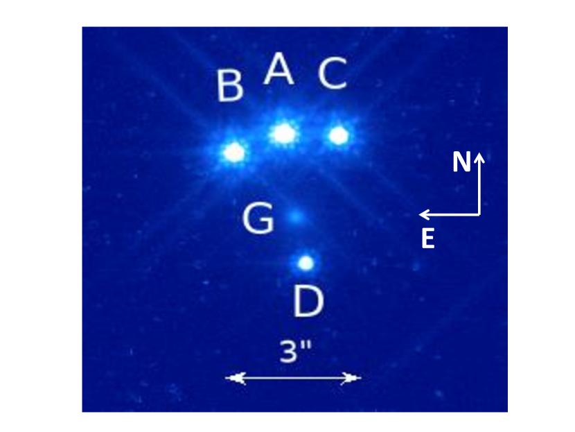
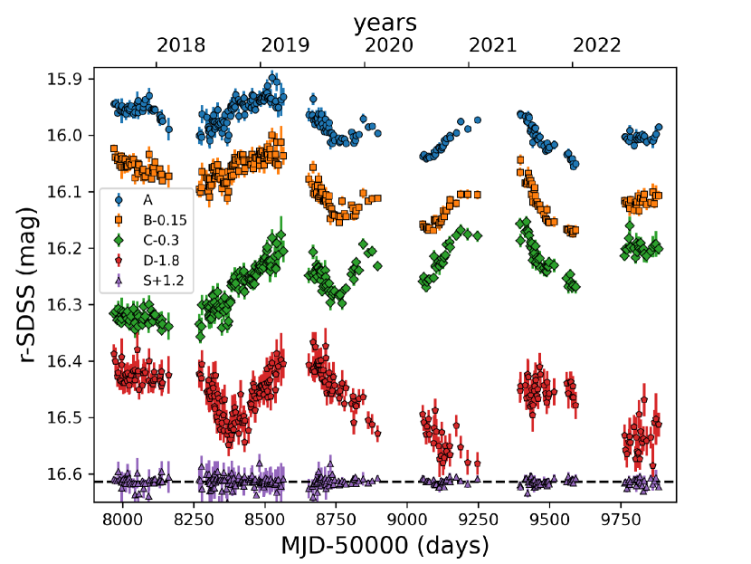
Figure 1: Left: Quasar images ABCD and main lens galaxy G of PS J0147+4630 from a public $HST$–WFC3 frame of the system in the $F814W$ band. Right: LT–NOT light curves of PS J0147+4630 from its discovery to 2022 October 30. The $r$–band magnitudes of images B, C, and D, and the control star are offset by $-$0.15, $-$0.3, $-$1.8, and +1.2, respectively, to facilitate comparison between them and with image A.

We also selected six non–variable blue stars in the field of PS J0147+4630 (catalog ) and performed PSF photometry on five of them (see the calibration stars Cal1–Cal5 in Table 1; Cal6 is a saturated star in LT frames). For each of the five calibration stars, we calculated its average magnitude within the monitoring period and magnitude deviations in individual frames (by subtracting the average). In each individual frame, the five stellar magnitude deviations were averaged together to calculate a single magnitude offset, which was then subtracted from the magnitudes of quasar images. After this photometric calibration, we removed 22 observing epochs in which quasar magnitudes deviate appreciably from adjacent values. Thus, the final LT $r$–band light curves are based on 190 frames (epochs), and the typical uncertainties in the light curves of the quasar images and control star (see Table 1) were estimated from magnitude differences between adjacent epochs separated by no more than 4.5 d (2019ApJ...887..126G). We derived typical errors of 0.0062 (A), 0.0077 (B), 0.0097 (C), 0.0197 (D), and 0.0058 (control star) mag. For the control star, we have also verified that its typical error practically coincides with the standard deviation of all measures (0.0055 mag). To obtain photometric uncertainties at each observing epoch, the typical errors were scaled by the relative signal–to–noise ratio of the PSF star (2000hccd.book.....H).

The optical monitoring of PS J0147+4630 (catalog ) with the NOT spanned from 2017 August to 2019 December. We used the ALFOSC camera with a pixel scale of $\sim$0$\farcs$21 and the $R$–Bessel filter. This passband is slightly redder than the Sloan $r$ band. Each observing night, we mainly took three exposures of 30 s each under good seeing conditions. The full–width at half–maximum (FWHM) of the seeing disc was about 1$\farcs$0 (we also estimated FWHM seeing = 1$\farcs$35 $\pm$ 0$\farcs$15 from LT frames), and we collected 298 individual frames over the entire monitoring campaign. After a standard data reduction, IMFITFITS PSF photometry yielded magnitudes for the quasar images (see above for details on the photometric model). To avoid biases in the combined LT–NOT light curves, the same photometric method was applied to LT and NOT frames. This method differs from that of MScKD, who used the DAOPHOT package in IRAF (1987PASP...99..191S; TRMD) to extract magnitudes from NOT frames.

The six calibration stars in Table 1 were used to adequately correct quasar magnitudes (see above), and we were forced to remove 17 individual frames leading to magnitude outliers. We then combined $R$–band magnitudes measured on the same night to obtain photometric data of the lensed quasar and control star at 77 epochs. Again, typical errors were derived from magnitudes at adjacent epochs that are separated $<$ 4.5 d. This procedure led to uncertainties of 0.0122 (A), 0.0122 (B), 0.0144 (C), 0.0197 (D), and 0.0170 (control star) mag. Errors at each observing epoch were calculated in the same way as for the LT light curves.

As a last step, we combined the $r$–band LT and $R$–band NOT light curves. If we focus on the quasar images and consider $rR$ pairs separated by no more than 2.5 d, the values of the average colour $\langle r-R\rangle$ are 0.0565 (A), 0.0616 (B), 0.0546 (C), and 0.0652 (D). Brightness records of the ABC images are more accurate than those of D, and thus we reasonably take the average colours of ABC to estimate a mean $r-R$ offset of 0.0576 mag. After correcting the $R$–band curves of the quasar for this offset, we obtain the new records in Table 2. Table 2 contains $r$–band magnitudes of the quasar images and the control star at 267 observing epochs (MJD$-$50 000). In Figure 1, we also display our new 5.2–year light curves.

3 Time delays and microlensing signals

Previous efforts focused on early monitorings with a single telescope, trying to estimate delays between the image A and the other quasar images, $\Delta t_{\rm{AX}}=t_{\rm{A}}-t_{\rm{X}}$ (X = B, C, D), and find microlensing signals (MScKD; 2019ApJ...887..126G). Here, we use the new light curves in Section 2 along with state–of–the–art curve–shifting algorithms to try to robustly measure time delays between images. At the end of this section, we also discuss the extrinsic (microlensing) variability of the quasar.

As is clear from Figure 1, there are short time delays between images ABC, while it is hard to get an idea about the $\Delta t_{\rm{AD}}$ value by eye. Fortunately, there are several cross–correlation techniques to measure time delays between light curves containing microlensing variations (e.g., 2015ApJ...800...11L, and references therein), and thus we considered PyCS3 curve–shifting algorithms (2013A&A...553A.120T; PyCS3; 2020A&A...640A.105M) to obtain reliable time delays of PS J0147+4630 (catalog ). PyCS3 is a well–tested software toolbox to estimate time delays between images of gravitationally lensed quasars, and we focused on the $\chi^{2}$ technique, assuming that the intrinsic signal and the extrinsic ones can be modelled as a free–knot spline (FKS). This technique shifts the four light curves simultaneously (ABCD comparison) to better constrain the intrinsic variability, and relies on an iterative nonlinear procedure to fit the four time shifts and splines that minimise the $\chi^{2}$ between the data and model (2013A&A...553A.120T). Results depend on the initial guesses for the time shifts, so it is necessary to estimate the intrinsic variance of the method using a few hundred initial shifts randomly distributed within reasonable time intervals. In addition, a FKS is characterised by a knot step, which represents the initial spacing between knots. The model consists of an intrinsic spline with a knot step $\eta$ and four independent extrinsic splines with $\eta_{\rm{ml}}$ that account for the microlensing variations in each quasar image (2020A&A...640A.105M).

To address the intrinsic variability, we considered three $\eta$ values of 30, 50 and 70 d. Intrinsic knot steps shorter than 30 d fit the observational noise, whereas $\eta$ values longer than 70 d do not fit the most rapid variations of the source quasar. Intrinsic variations are usually faster than extrinsic ones, and additionally, the software works fine when the microlensing knot step is significantly longer than $\eta$. Therefore, the microlensing signals were modelled as free–knot splines with $\eta_{\rm{ml}}$ = 350$-$400 d (i.e., values intermediate between those shown in Table 2 of 2020A&A...640A.105M). We also generated 500 synthetic (mock) light curves of each quasar image, optimised every mock ABCD dataset, and checked the similarity between residuals from the fits to the observed curves and residuals from the fits to mock curves. The comparison of residuals was made by means of two statistics: standard deviation and normalised number of runs $Z_{\rm{r}}$ (see details in 2013A&A...553A.120T). For $\eta$ = 50 d and $\eta_{\rm{ml}}$ = 400 d, histograms of residuals derived from mock curves (grey) and from the LT–NOT light curves of PS J0147+4630 (catalog ) are included in the top panels of Figure 2. It is apparent that the standard deviations through the synthetic and the observed curves match very well. Additionally, the bottom panels of Figure 2 show distributions of $Z_{\rm{r}}$ from synthetic light curves (grey) for $\eta$ = 50 d and $\eta_{\rm{ml}}$ = 400 d. These bottom panels also display the $Z_{\rm{r}}$ values from the observations (vertical lines), which are typically located at $\sim$0.4$\sigma$ of the mean values of the synthetic distributions.

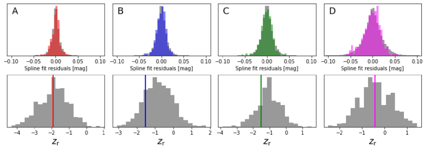
Figure 2: Top: Distributions of FKS fit residuals for $\eta$ = 50 d and $\eta_{\rm{ml}}$ = 400 d. The grey histograms represent the distributions of residuals from the fits to 500 synthetic light curves of each image, while the red, blue, green and magenta histograms correspond to the distributions of residuals from the fits to the LT–NOT light curves. Bottom: Normalised number of runs $Z_{\rm{r}}$ for the synthetic data (grey histograms) and the observed brightness records (red, blue, green and magenta vertical lines).

Four pairs of ($\eta$, $\eta_{\rm{ml}}$) values (see above) led to the set of time delays in Figure 3. We have verified that other feasible choices for $\eta_{\rm{ml}}$ (e.g., $\eta_{\rm{ml}}$ = 200 d) do not substantially modify the results in this figure. The black horizontal bars correspond to 1$\sigma$ confidence intervals after a marginalisation over results for all pairs of knot steps, and those in the left panels and bottom panels of Figure 3 are included in Table 3. We finally adopted the time delays in Table 3, which are symmetric about central values and useful for subsequent studies.

It seems to be difficult to accurately determine delays between the brightest images ABC because they are really short. To robustly measure $\Delta t_{\rm{AC}}$ in a near future, we will most likely need to follow a non–standard strategy focused on several time segments associated with strong intrinsic variations and weak extrinsic signals. Fortunately, we find an accurate and reliable value of $\Delta t_{\rm{AD}}$ (uncertainty of about 4%), confirming the early result from two monitoring seasons with the NOT and a technique different to that we used in this paper (MScKD). It is also worth mentioning that the dispersion method ignoring microlensing variations (the simplest approximation with fewer free parameters; 1996A&A...305...97P) produces an optimal AD delay separated by only 10 days from that obtained with PyCS3. We also note that $\Delta t_{\rm{BD}}$ and $\Delta t_{\rm{CD}}$ have errors of 3.5$-$3.7%, and thus we present accurate values of the three independent time delays relative to image D.

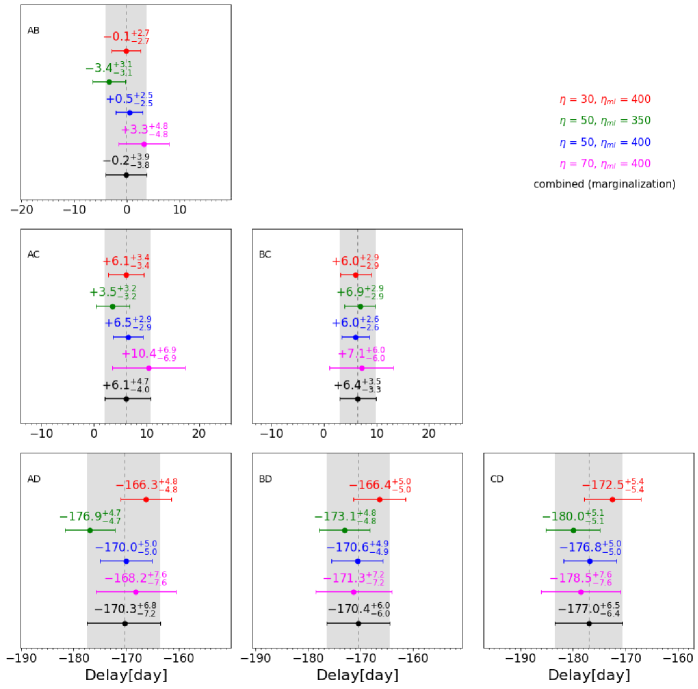
Figure 3: Time–delay estimates using the $\chi^{2}$ technique and free–knot splines. Combined estimates ($\tau_{\rm{thresh}}$ = 0; 2018A&A...616A.183B) are highlighted with grey rectangles encompassing the individual measurements.

Table 3: Time delays of PS J0147+4630.

$\Delta t_{\rm{AB}}$	$\Delta t_{\rm{AC}}$	$\Delta t_{\rm{AD}}$	$\Delta t_{\rm{BD}}$	$\Delta t_{\rm{CD}}$
$-$0.2 $\pm$ 3.9	+6.4 $\pm$ 4.4	$-$170.5 $\pm$ 7.0	$-$170.4 $\pm$ 6.0	$-$177.0 $\pm$ 6.5

Note. — Here, delays $\Delta t_{\rm{YX}}=t_{\rm{Y}}-t_{\rm{X}}$ are in days, image Y leads image X if $\Delta t_{\rm{YX}}<$ 0 (otherwise Y trails X), and all measurements are 68% confidence intervals. We combined the individual measures of $\Delta t_{\rm{YX}}$ from PyCS3 (see Figure 3) and then made symmetric error bars.

An image comparison spanning 13 years is also depicted in Figure 4. We have downloaded five $r$–band warp frames of PS J0147+4630 (catalog ) that are included in the Data Release 2 of Pan–STARRS. These Pan–STARRS frames were obtained on three nights in the 2010$-$2013 period, i.e., a few years before the discovery of the lens system. Two frames are available on two of the three nights, so rough photometric uncertainties through average intranight variations are 0.012 (A), 0.008 (B), 0.019 (C), and 0.033 (D) mag. To discuss the differential microlensing variability of the images BCD with respect to A, Figure 4 shows the original curve of A along with shifted curves of BCD. We used the central values of the delays relative to image A and constant magnitude offsets to shift curves. The offsets $\Delta m_{\rm{AB}}$, $\Delta m_{\rm{AC}}$, and $\Delta m_{\rm{AD}}$ are average differences between magnitudes of A and those of B, C, and D, respectively. The global shapes of the four brightness records indicate the presence of long–term microlensing effects and suggest that PS J0147+4630 (catalog ) is a suitable target for a deeper analysis of its microlensing signals. Over the last six years, it is noteworthy that there is good overlap between the original curve of A and the shifted curve of D. In addition, the differential microlensing variation of C is particularly prominent, showing a microlensing episode with a total amplitude greater than 0.1 mag.

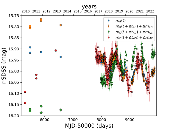
Figure 4: LT–NOT data (smaller symbols) plus photometric data from Pan-STARRS $r$–band frames in 2010$-$2013 (larger symbols). The original brightness record of A is compared with shifted light curves of B, C, and D. To shift the BCD light curves, we apply the corresponding time delays and constant magnitude offsets (see main text for details).

4 Lens mass models and Hubble constant

2017ApJ...844...90B presented preliminary modelling of the lens mass of PS J0147+4630 (catalog ) from Pan–STARRS data, whereas 2019MNRAS.483.5649S; 2021MNRAS.501.2833S have recently modelled the lens system using $HST$ imaging. To model the $HST$ images, Shajib et al. have considered the distributions of light of the lens and source, and the lens mass distribution. Their solution for the lensing mass relies on a lens scenario consisting of a singular power–law ellipsoid (SPLE; describing the gravitational field of the main lens galaxy G) and an external shear (ES; accounting for the gravitational action of other galaxies). The dimensionless surface mass density (convergence) profile of the SPLE was characterised by a power–law index $\beta$ = 2.00 $\pm$ 0.05, where $\beta$ = 2 for an isothermal ellipsoid.

We first considered Shajib et al.’s solution, a flat $\Lambda$CDM (standard) cosmology with matter and dark energy densities of $\Omega_{\rm{M}}$ = 0.3 and $\Omega_{\Lambda}$ = 0.7, respectively, updated redshifts $z_{\rm{l}}$ = 0.678 (2019ApJ...887..126G) and $z_{\rm{s}}$ = 2.357 (based on emission lines that are observed at near–-IR wavelengths), and the time delay in the third column of Table 3 to calculate $H_{0}^{\rm{model}}$ and put it into perspective. We obtained $H_{0}^{\rm{model}}$ = 100 $\pm$ 10 km s${}^{-1}$ Mpc${}^{-1}$, which significantly exceeds a concordance value of $\sim$70 km s${}^{-1}$ Mpc${}^{-1}$ (e.g., 2015LRR....18....2J). If additional mass along the line of sight is modelled as an external convergence $\kappa_{\rm{ext}}$, then $H_{0}^{\rm{true}}=H_{0}^{\rm{model}}(1-\kappa_{\rm{ext}})$ (e.g., 2017MNRAS.467.4220R). The factor $1-\kappa_{\rm{ext}}$ should be $\sim$0.7 ($\kappa_{\rm{ext}}\sim$ 0.3) to decrease $H_{0}$ until accepted values. Therefore, the external convergence required to solve the $H_{0}$ crisis is an order of magnitude higher than typical values of $\kappa_{\rm{ext}}$ (e.g., 2017MNRAS.467.4220R; 2020A&A...643A.165B).

The Hubble constant can be also inferred from another lens mass solution based on approaches similar to those of Shajib et al. Adopting a standard cosmology and updated redshifts (see above), the solution of 2023MNRAS.518.1260S and the three time delays relative to image D (last three columns in Table 3) led to $H_{0}^{\rm{model}}$ values in the range 116 to 131 km s${}^{-1}$ Mpc${}^{-1}$. Thus, Schmidt et al.’s solution with power–law index $\beta$ = 2.08 $\pm$ 0.02 produces even higher $H_{0}^{\rm{model}}$ values than those from Shajib et al.’s solution. Although the $H_{0}$ crisis may be related to an inappropriate (SPLE + ES) lens scenario or a very high external convergence, we have sought for a new mass reconstruction using astrometric and time–delay constraints, a SPLE + ES scenario, updated redshifts, a standard cosmology, and $H_{0}^{\rm{model}}$ = 70 km s${}^{-1}$ Mpc${}^{-1}$. In presence of a typical (weak) external convergence, the $H_{0}^{\rm{true}}$ value would be consistent with accepted ones.

Our standard astrometric constraints consisted of the $HST$ positions of ABCD (with respect to G at the origin of coordinates; 2019MNRAS.483.5649S; 2021MNRAS.501.2833S). SPLE + ES mass models of quads usually indicate the existence of an offset between the centre of the SPLE and the light centroid of the galaxy (e.g., 2012A&A...538A..99S; 2019MNRAS.483.5649S; 2021MNRAS.501.2833S). Hence, instead of formal astrometric errors for G, we adopted $\sigma_{x}$ = $\sigma_{y}$ = 0$\farcs$04. This uncertainty level equals the root–mean–square of mass/light positional offsets for most quads in the sample of Shajib et al. In addition to astrometric data, the set of constraints incorporated the LT–NOT time delays relative to image D (see Table 3). The number of observational constraints and the number of model parameters were 13 and 10, respectively. For three degrees of freedom, the GRAVLENS/LENSMODEL software (2001astro.ph..2340K; gravlensmanual) led to the 1$\sigma$ intervals in Table 4 ($\chi^{2}$ = 3.56 for the best fit).

Table 4: SPLE + ES mass model of PS J0147+4630.

$\beta$	$b$ (″)	$e$	$\theta_{e}$ (°)	$\gamma$	$\theta_{\gamma}$ (°)
1.86 $\pm$ 0.07	1.878 $\pm$ 0.018	0.170 $\pm$ 0.045	$-$70.8 $\pm$ 3.5	0.177 $\pm$ 0.019	10.8 $\pm$ 0.7

Note. — We consider $HST$ astrometry and LT–NOT time delays as constraints. We also adopt updated redshifts, a standard cosmology, and $H_{0}^{\rm{model}}$ = 70 km s${}^{-1}$ Mpc${}^{-1}$. Position angles ($\theta_{e}$ and $\theta_{\gamma}$) are measured east of north, and $\beta$, $b$, $e$, and $\gamma$ denote power–law index, mass scale and ellipticity of the SPLE, and external shear strength, respectively. We show 68% (1$\sigma$) confidence intervals.