Viewing the process of generating counterfactuals as a source of knowledge

Abstract

There are now many explainable AI methods for understanding the decisions of a machine learning model. Among these are those based on counterfactual reasoning, which involve simulating features changes and observing the impact on the prediction. This article proposes to view this simulation process as a source of creating a certain amount of knowledge that can be stored to be used, later, in different ways. This process is illustrated in the additive model and, more specifically, in the case of the naive Bayes classifier, whose interesting properties for this purpose are shown.

I Introduction

Machine learning, one of the branches of artificial intelligence, has enjoyed many successes in recent years. The decisions made by these models are increasingly accurate, but also increasingly more complex. However, it appears that some of these models are like black boxes: their decisions are difficult, if not impossible, to explain [1]. This lack of explainability can lead to a number of undesirable consequences: lack of user confidence, reduced usability of the models, presence of biases, etc. These needs have given rise to the field of XAI (eXplainable AI). XAI [2, 3] is a branch of artificial intelligence that aims to make the decisions made by machine learning models intelligible, understandable, to users.

Among XAI methods, some of them are based on counterfactual reasoning. Counterfactual reasoning is a concept from psychology and social sciences [4], that involves examining possible alternatives to past events [5]. Humans often use counterfactual reasoning by imagining what would happen if an event had not occurred, and this is exactly what counterfactual reasoning is. Applied to artificial intelligence, the question is, for example, “Why did the model make this decision rather than another?” (counterfactual explanation) or “How would the decision have been different if a certain condition had been changed?”. This reasoning can take the form of a counterfactual or semi-factual explanation.

A counterfactual explanation might be “If your income had been greater by $10000 then your credit would have been accepted” [6]. A semi-factual is a special-case of the counterfactual in that it conveys possibilities that “counter” what actually occurred, even though the outcome does not change [7]: “Even if your income had been greater by $5000 your credit is still rejected” (but closer to be accepted), see Figure 1.

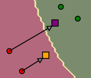
Figure 1: Illustration of a counterfactual and a semi-factual. The red dots represent initial examples ($X$). The orange represents a semi-factual, the purple point represents a counterfactual and the white line represents the decision boundary between the red class and the green class.

Within the framework of counterfactual reasoning, this article proposes to consider both feature changes, and its impact on the prediction, as a source of knowledge that can be stored and then exploited in diverse ways. This process is illustrated in the case of additive models and in particular in the case of the naive Bayes classifier, whose interesting properties for this purpose will be shown.

The rest of this paper is organized as follows: Section II explains (i) how to build a knowledge base from a classifier by using counterfactual reasoning and (ii) how deriving explanations from this knowledge base and (iii) some other additional usable knowledge. Section III presents a concrete implementation to elaborate the knowledge base in the case of the naive Bayes classifier. The Section IV illustrates, by means of an unsubscribing problem, (i) how clustering applied to this database generates new knowledge and (ii) examples of use of the database to create trajectories to transform initial example to counterfactual or semi-factual. Finally the last section concludes this paper.

II Creation and use of a knowledge base

In this section, we introduce the notations, that are necessary for understanding the contribution. Then we explain how to build a knowledge base from a classifier by using counterfactual reasoning. Finally, we present the different types of explanations that can be derived from the knowledge base.

II-A Backgrounds

Let $f$ be a predictive model that is trained using $N$ examples, each described by a set of $d$ explanatory variables (a vector $X=\{X_{1},....,X_{d}\}$, derived from a $\mathcal{X}$ distribution) so as to predict a categorical target variable denoted $Y=\{y_{1},...,y_{K}\}$ derived from a $\mathcal{Y}$ distribution. We assume that the dataset taken as input by the classifier is discretised, meaning that each variable $x_{i}$ falls into an interval of values $I_{q}$, where $q$ is the $q-th$ interval of values.

II-B Creation of the knowledge base

Our goal is to build a table that stores each variable change and its impact on the prediction. Since the dataset is discretised, each variable change is represented by the membership to a new interval of values. To measures the difference in prediction, we propose to use the predicted probability returned by the classifier. Table I gives an example of a such table in the case of two variables $X_{1}$ and $X_{2}$ respectively discretised (or grouped) into 2 and 3 intervals (groups) of values ($I$). For each individual, $l$, each row of the table, we store differences in predicted probabilities values where $\Delta(X^{l}_{i,*\rightarrow m},X^{l})$ is the difference in predicted probability for class 1, when the value of variable $i$ is changed from its initial value $`*^{\prime}$ to the value of interval (group) $m$ (simplified as $\Delta(X^{l}_{i,*\rightarrow m})$ in the table).

	$X_{1}$		$X_{2}$
	$I_{1}$	$I_{2}$	$I_{1}$	$I_{2}$	$I_{3}$
${X^{1}}$	$\Delta({X^{1}_{1,*\rightarrow 1}})$	$\Delta({X^{1}_{1,*\rightarrow 2}})$	$\Delta({X^{1}_{2,*\rightarrow 1}})$	$\Delta({X^{1}_{2,*\rightarrow 2}})$	$\Delta({X^{1}_{2,*\rightarrow 3}}$
${X^{2}}$	$\Delta({X^{2}_{2,*\rightarrow 1}})$	$\Delta({X^{2}_{2,*\rightarrow 2}})$	$\Delta({X^{2}_{2,*\rightarrow 1}})$	$\Delta({X^{2}_{2,*\rightarrow 2}})$	$\Delta({X^{2}_{2,*\rightarrow 3}})$

TABLE I: Illustration of the knowledge base, here in the case of two variables and two examples.

To effectively exploit this knowledge base, the classifier that is used needs to have an additivity property regarding the prediction. This means that individual differences in predicted probabilities can be summed to obtain the overall difference in predicted probability. More formally, let $X_{i}$ and $X_{j}$ being two variables and $m,p$ being two new values of interval for each variable, respectively.

Then a classifier is considered as additive if for each individual $l$:

$$\medmath{\Delta(X^{l}_{(i,*\rightarrow m)},X^{l})+\Delta(X^{l}_{(j,*\rightarrow p)},X^{l})=\Delta(X^{l}_{(i,*\rightarrow m)\cup(j,*\rightarrow p)},X^{l})}$$

where $\Delta(X^{l}_{(i,*\rightarrow m)\cup(j,*\rightarrow p)},X^{l})$ is the difference in predicted probability for class 1 when both variable $i$ and $j$ are changed.

We will show in Section III that this property holds for the naive Bayes classifier. However, this choice as no limitation, since every other classifier that holds this property can be used.

II-C Deriving explanations from the knowledge base

After building this knowledge base, different types of explanations can be derived, such as counterfactual or semi-factual explanation. Moreover, we introduce two new types of explanations that are trajectories and profile clustering.

II-D Counterfactual explanation

In the explainable AI setting, a counterfactual explanation is defined as the smallest change of feature values that changes the prediction of a model to a given output. An example of a counterfactual explanation can be ”if your monthly income had been $500\$$ higher, then your credit would have been accepted”. The new example that is obtained by changing the feature income by $500\$$ is called a counterfactual. Many methods have been proposed to generate counterfactuals, focusing on some specific properties such as realism  [8, 9, 10], actionability [11, 12], sparsity  [13, 14], or robustness  [15].

II-D1 Generating sparse counterfactuals

The sparsity property involves having counterfactuals with the smallest number of modified variables. Sparse explanation are interesting because they are more comprehensible for human [16] and also more actionable, i.e. the change proposed by the counterfactual is easier to be implemented. Such explanations can be easily obtained by exploiting our knowledge base. For a given individual, $X$, all we have to do is read the value of the largest $\Delta$ and then, as we have the additivity property, read the second value of the largest $\Delta$ for a second variable and so on. At each stage we check whether ($f(\mathbf{X^{\prime}})>0.5$). If this is the case, the counterfactual has been found .

II-D2 Taking into account other properties

In other cases, the aim may be to find the closest counterfactual, but under ‘business constraints’ defined by the user. For example, the search for counterfactuals could be restricted to making changes only in adjacent intervals (e.g. intervals of close values). Given the table I, we would be allowed to move people from interval 1 to 2 for the second variable, but not from 1 to 3. The user can also constrain the search by requiring that one of the variables must always be changed to a certain value, and so on. This type of constraint can easily be considered and incorporated into a counterfactual search algorithm using the proposed knowledge table.

The literature on counterfactuals sets out some interesting properties on the subject, such as (i) the notion of minimality: having a counterfactual that differs as little as possible from the original example; (ii) realism: the generated counterfactual must not contain changes that do not make sense from the point of view of the data (e.g. a decrease in the “age” of an individual), also known as plausibility [17]; (iii) generating counterfactuals that are similar to real examples or in dense regions of the class of interest, in order to have robust counterfactuals [15].

Note that a lot of these different properties can be easily achieved by exploiting the knowledge base differently, since the user can select the variables he wishes to intervene on, based on the criterion of his choice.

II-E Additional usable knowledge

II-E1 Preventive and reactive actions -

So far, we have mainly talked about creating counterfactuals to explain the model’s decisions (as mentioned in the introduction to this article), but also potentially to be able to take reactive actions. For example, if a bank customer is predicted to “leave” (churner), the counterfactual example indicates one or more actions that should be taken in order to try to keep him as a customer: these are known as “reactive” actions.

Conversely, the study of counterfactual trajectories a posteriori is of great interest, as it also allows us to identify when a trajectory is approaching the frontier (see Figure 2).

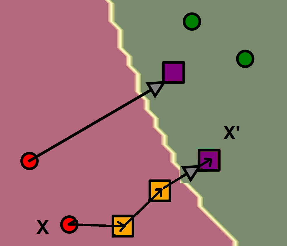
Figure 2: Illustration of two counterfactuals: one achieved in 1 step, the second in 3 steps

In such situations, reactive measures can be taken to reverse the trend and avoid undesirable outcomes (for example by observing the second step of the trajectory at the bottom of the figure 2). This approach is particularly relevant when it comes to predicting churn, for example, as it enables us to identify customers who are “starting” to churn. By being proactive, it is possible to put in place targeted strategies to retain these customers and bring them back to a quality service.

Finally, our knowledge base can also be used to carry out “preventive” actions. Going back to Figure 1, we can try to create a (negative) semi-factual which moves away from the decision frontier (see Figure 3) : ”The customer is not predicted as leaving but is nevertheless close to the decision frontier”. In this case, all we need to do is look at the negative values of $\Delta$ and take steps away from it according to the user’s wishes. For example, all the people who are one step away from crossing the decision frontier, who are easily identifiable in this case, could be concerned.

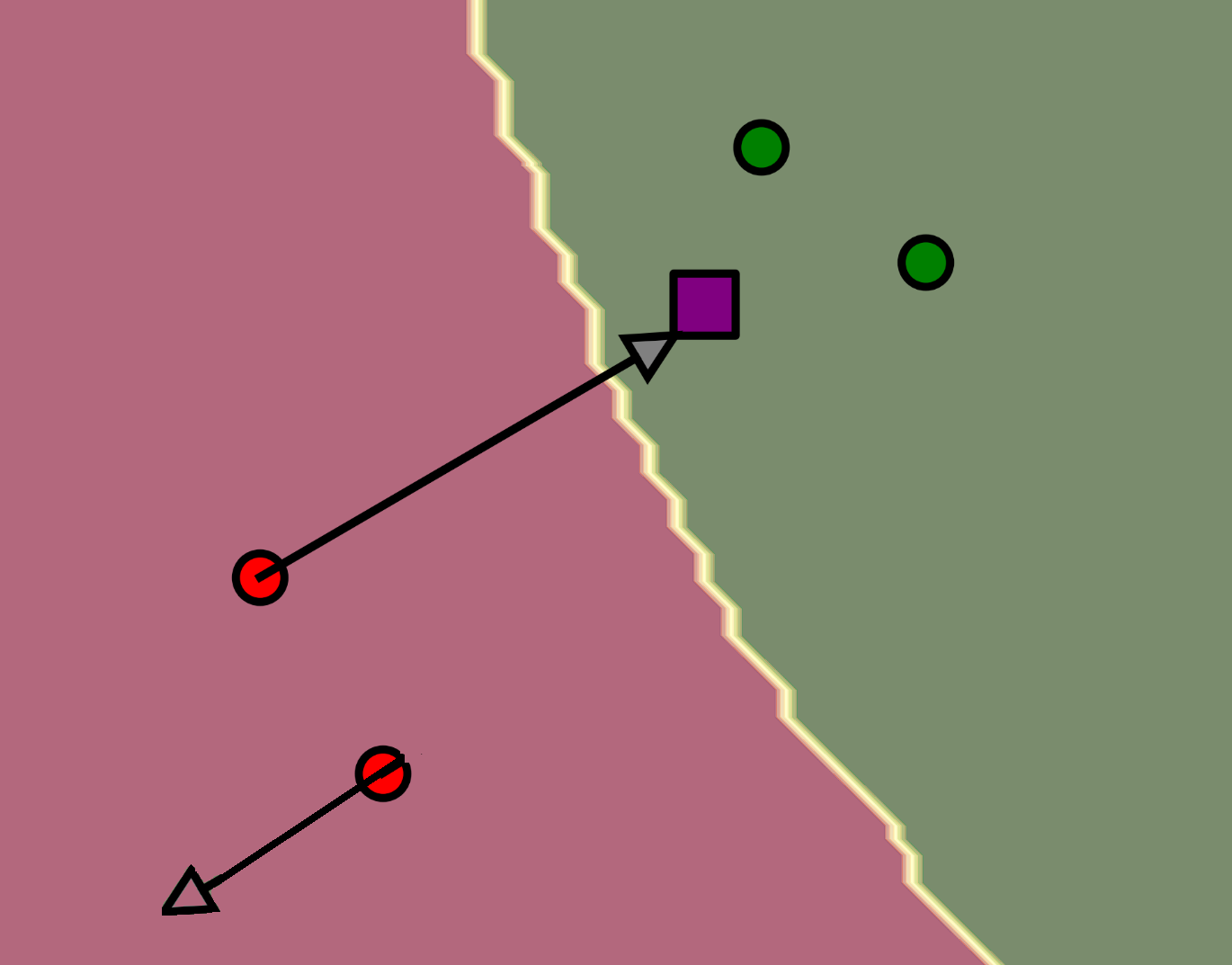
Figure 3: Illustration of a counterfactuals (on top) and a “negative” semi-factual (bottom) which moves away from the decision frontier

II-E2 Profile creation -

The last way of using the knowledge base that we will describe here, is to carry out an exploratory analysis using a clustering technique.

Using the knowledge base, it is possible to group individuals according to the impact of each possible change, i.e. the impact resulting from each of these changes. Analysis of the created clusters can be a source of learning. This is illustrated in the next section.

Note: all uses of the knowledge base, presented in this paper, are on-demand, local, global or in-between, to generate uses for both counterfactual and semi-counterfactual allowing for a wide range of uses.

III Computing $\Delta$ in the case of the naive Bayes classifier

III-A Reminders on the naive Bayes classifier

The naive Bayes classifier (NB) is a widely-used tool in supervised classification problems. It has the advantage of being efficient for many real data sets [18]. However, the naive assumption of conditional independence of the variables can, in some cases, degrade the classifier’s performance. This is why variable selection methods have been developed [19]. They mainly consist of variable addition and deletion heuristics to select the best subset of variables maximizing a classifier performance criterion, using a wrapper-type approach [20]. It has been shown in [21] that averaging a large number of selective naive Bayes classifiers, performed with different subsets of variables, amounts to considering only one model with a weighting on the variables. Bayes’ formula under the assumption of independence of the input variables conditionally to the class variable becomes:

$$P(C_{k}|X)=\frac{P(C_{k})\prod_{i}P(X_{i}|C_{k})^{W_{i}}}{\sum_{j=1}^{K}(P(C_{j})\prod_{i}P(X_{i}|C_{j})^{W_{i}})}$$ (1)

where $W_{i}\in[0,1]$ is the weight of variable $i$. The predicted class is the one that maximizes the conditional probability $P(C_{k}|X)$. The probabilities $P(X_{i}|C_{i})$ can be estimated by intervals using discretization for numerical variables. Gaussian naive Bayes could be also considered. For categorical variables, this estimation can be done directly if the variable takes few different modalities, or after grouping (of values) in the opposite case.

III-B Criteria to be optimized in the search for counterfactuals

Let, $X$ as an example, and two classes $C_{1}$ and $C_{2}$. The search for a counterfactual consists in optimizing and increasing the probability of belonging to the target class $C_{1}$ when $X$ is initially predicted by the model to belong to $C_{2}$ (and vice versa). To do this, we can develop a gluttonous algorithm, which is expensive in terms of computation time and does not necessarily have the additivity properties described above. We propose below to pose the problem differently, rewriting the equation 1 and looking at how to increase the probability of belonging to a particular class of interest. To achieve this goal, and to maximize $P(C_{j}|X^{\prime})$ with respect to the initial value of $P(C_{j}|X)$, we will exploit the following proposition:

If we take $X$ and $X^{\prime}$ as two elements of the input space $\mathcal{X}$, we show that for a two-class classification problem, searching for counterfactuals of $X$ amounts to examining the evolution of the value of $\Delta$ when we change some of the values of $X$ to $X^{\prime}$, such that:

$$\begin{split}\Delta(X,X^{\prime})&=\left(\sum_{i=1}^{d}W_{i}(\log{P(X_{i}|C_{1})}-\log{P(X_{i}|C_{2})})\right)\\ &-\left(\sum_{i=1}^{d}W_{i}(\log{P(X^{\prime}_{i}|C_{1})}-\log{P(X^{\prime}_{i}|C_{2})})\right)\end{split}$$ (2)

Proof: If we start again from the equation 1

$$P(C_{j}|{X})=\frac{P(C_{j})\prod_{i=1}^{d}P(X_{i}|C_{j})^{W_{j}}}{\sum_{z}[P(C_{z})\prod_{i=1}^{d}P(X_{i}|C_{z})^{W_{j}}]}$$ (3)

by posing:

$$\begin{split}L_{j}({X})&=\log\left(P(C_{j})\prod_{i=1}^{d}P(X_{i}|C_{j})^{W_{i}}\right)\\ &=\log{P(C_{j})}+\sum_{i=1}^{d}W_{i}\log{P(X_{i}|C_{j})}\end{split}$$ (4)

then we have:

$$\begin{split}P(C_{j}|{X})&=\frac{e^{L_{j}({X})}}{\sum_{z}e^{L_{z}({X})}}\\ &=\frac{1}{\sum_{z}e^{L_{z}({X})-L_{j}({X})}}\\ &=\frac{1}{1+\sum_{z\neq j}e^{L_{z}({X})-L_{j}({X})}},\end{split}$$ (5)

and so in the case of two classes:

$$P(C_{j}|{X})=\frac{1}{1+e^{L_{j^{\prime}}({X})-L_{j}({X})}}$$ (6)

We can see that to get closer to the class $C_{j}$, all we have to do is reduce the quantity $L_{j^{\prime}}({X})-L_{j}({X})$, and thus reduce:

$$\begin{split}\log{P(C_{j^{\prime}})}+\sum_{i=1}^{d}W_{i}\log{P(X_{i}|C_{j^{\prime}})}\\ -\log{P(C_{j})}-\sum_{i=1}^{d}W_{i}\log{P(X_{i}|C_{j})}\end{split}$$ (7)

Since $P(C_{j})$ and $P(C_{j^{\prime}})$ are constant, this is equivalent to decreasing:

$$\sum_{i=1}^{d}W_{i}\log{P(X_{i}|C_{j^{\prime}})}-\sum_{i=1}^{d}W_{i}\log{P(X_{i}|C_{j})}$$

and therefore to take an interest in the distance:

$$\begin{split}\Delta({X},{X^{\prime}})&=\sum_{i=1}^{d}W_{i}(\log{P(X_{i}|C_{j^{\prime}})}-\log{P(X_{i}|C_{j})})\\ &-\sum_{i=1}^{d}W_{i}(\log{P(X^{\prime}_{i}|C_{j^{\prime}})}-\log{P(X^{\prime}_{i}|C_{j})})\end{split}$$ (8)

If $\Delta$ is positive then we are getting closer to the decision frontier (or even crossing it) if $\Delta$ is negative then we are moving away from the decision frontier and therefore away from the desired objective. The counterfactual search algorithm becomes straightforward. Simply calculate, for a given example $X$, the value of $\Delta$ for each explanatory variable and for each value of this explanatory variable. Then, given these values, iterate the successive changes in order to obtain a counterfactual example. These variable-by-variable changes have the property of being additive.

Indeed, if we consider four examples $X^{0}$, $X^{{}^{\prime}1}$, $X^{{}^{\prime}2}$ and $X^{{}^{\prime}3}\in\mathcal{X}$, which are respectively (i) an initial example $X^{0}$, then the same example for which we have modified only one explanatory variable $l$ for $X^{{}^{\prime}1}$, $m$ for $X^{{}^{\prime}2}$, and finally an example that cumulates the two univariate modifications $l$ and $m$ for $X^{{}^{\prime}3}$, such that :

$$\exists!\ l\ \text{such as}\ X^{{}^{\prime}1}_{l}\neq X^{0}_{l}$$

$$\exists!\ m\ \text{such as}\ X^{{}^{\prime}2}_{m}\neq X^{0}_{m}\ \text{and}\ m\neq l$$

and

$$X^{{}^{\prime}3}_{k}=\begin{cases}X^{{}^{\prime}1}_{l},&\text{if }k=l\\ X^{{}^{\prime}2}_{m},&\text{if }k=m\\ X^{0}_{k},&\text{otherwise}\end{cases}$$

then it is obvious, from the additivity over all the variables in the equation 2, that we have : $\Delta({X_{0}},{X^{\prime}_{3}})=\Delta({X_{0}},{X^{\prime}_{1}})+\Delta({X_{0}},{X^{\prime}_{2}})$. Modifying one variable and then the other is equivalent to modifying them simultaneously in the calculation of $\Delta$. It should also be noted that this additivity is demonstrated from the equation 6, so we can be sure of increasing the normalized value of the probability of the class of interest, $P(C|X)$, which is a plus.

Note: The list of $\Delta$ values can potentially be very large if the number of distinct values of the explanatory variables is large. Nevertheless, it is common for some naive Bayes classifiers (except the Gaussian version) [22, 23] to discretise the numerical variables and group the modalities of the categorical variables, in a supervised manner, in order to obtain an estimate of the conditional densities ($P(X_{i}|C)$) which are then used in the calculation of $P(C|X)$. This is what has been done in this article using the [24] and [25] methods for numerical and categorical variables respectively. These supervised discretisation and grouping operations often produce a limited number of intervals or groups of modalities. This makes it possible to obtain a reasonable number of values to test.

IV Illustration on an unsubscribe case

IV-A Dataset and classifier used

This section uses the “Telco Customer Churn” dataset (widely-used in analyzing the results of XAI methods) provided by a fictitious telecommunications company that provided home telephone and internet services to 7043 customers in California. The aim is to classify people who may or may not leave the company. Each customer is described by 20 descriptive variables (3 numerical and 17 categorical) plus the class variable ‘churn’ (yes/no) which has two modalities (75% non-churn). This dataset can be downloaded from Kaagle [26]. We use 80% of the data for learning and 20% for testing. The naive Bayes classifier is produced using the Khiops library, which is available on Github [27], the rest of the computation is straightforward using Equation 8.

During the learning process, only 10 of the variables were retained in the model. Below are all the intervals of values or groups of modalities obtained during the pre-processing process (the value in brackets gives the weight of the variable in the model, equation 1, values from 0 to 1):

• 1 * - Tenure ($W_{1}$=0.67): [0-0.5], ]0.5-1.5], ]1.5-5.5], ]5.5-17.5], ]17.5-42.5], ]42.5-58.5], ]58.5-71.5], ]71.5-72]

• 2 - InternetService ($W_{2}$=0.78): [Fiberoptic], [DSL], [No]

• 3 - Contract ($W_{3}$=0.37): [Month-to-month], [Twoyear], [Oneyear]

• 4 - PaymentMethod ($W_{4}$=0.29): [Mailedcheck], [Creditcard(automatic), Electroniccheck, Banktransfer(automatic)]

• 5 - OnlineSecurity ($W_{5}$=0.15): [No], [Yes], [No internet service]

• 6 -TotalCharges ($W_{6}$=0.29): [18.8;69.225], ]69.225;91.2], ]91.2;347.9], ]347.9;1182.8],

  ]1182.8 ;2065.7], ]2065.7;3086.8], ]3086.8;7859], ]7859;8684.8]

• 7 * - PaperlessBilling ($W_{7}$=0.40): [Yes], [No]

• 8 - TechSupport ($W_{8}$=0.04): [No], [Yes], [No internet service]

• 9 * - SeniorCitizen ($W_{9}=0.28$): [0], [1]

• 10 * - Dependents ($W_{9}=0.10$): [Yes], [No]

For all 10 variables, there are a total of 36 intervals/groupings and therefore 26 values of $\Delta$ to calculate in our knowledge base. Indeed, for each individual and each variable, there is a $\Delta$ value that has a null value, the value which corresponds to it factually and which therefore does not need to be calculated.

IV-B Classifier analysis stage

Before carrying out the clustering stage, it is important to take an interest in the variables retained during the classification model training stage. For example, although it may be interesting to analyze the ‘Tenure’ variable, it is clearly not an actionable variable. Indeed, it is not possible to change a customer’s seniority in order to make him potentially less unfaithful. The same applies to the ‘SeniorCitizen’ and ‘Dependents’ variables. We have also removed the ‘PaperlessBilling’ variable, which has very little impact on the clustering results described below. As a result, these 4 variables are not retained during the clustering stage below; only the informative, influential and actionable variables are retained (see Section II-E1).

IV-C Exploratory Analysis using a clustering

IV-C1 Clustering performed

The clustering performed is usual: (i) we use the table of $\Delta$ values calculated on the test set, (ii) we learn a k-means with the L2 [28] distance for different $k$ values ($k\in\{2,12\}$), (iii) and finally we retain the k-means whose value of $k$ corresponds to the ‘elbow point’, here $k=4$, [29] of the curve representing the global reconstruction distance versus the value of $k$.

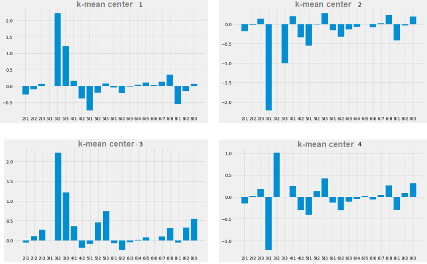
Figure 4: Average profile of individuals in clusters represented as histograms. The names of the values on the abscissa refer to the number of the variables and the number of the intervals (groups) described above. For example, ‘3I2’ refers to the third variable (’Contract’) and its second interval / group of values (’Twoyear’). The ordinate values are the mean values of the cluster ($\Delta$).

IV-C2 Results

The resulting clusters are shown in Figure 4. An analysis of these 4 clusters, combined with the predictions of the classifier, shows that:

• Cluster 1 (10% of the global population and containing 2% of customers predicted to be churner): individuals who can be made less churner mainly by means of variable 3 (‘Contract’) - i.e. by trying to get them to take out an annual contract (‘Twoyear’ or ‘OneYear’); NB - this marketing action is fairly difficult to carry out.

• Cluster 2 (24% of the global population and containing no customer predicted to be churner): people who are very insensitive to the fact that they are becoming less churner (mostly negative $\Delta$ means). They may not be targeted by a ‘reactive’ marketing campaign (which is in line with the classifier’s predictions), but rather by a preventive campaign using the ‘contract’ variable or the ‘payment method’ variable (payment by card or direct debit).

• Cluster 3 (45% of the global population and containing 47% of customers predicted to be churner (almost all of the individuals predicted to be churner)): some similarities with the individuals in cluster 1 for the ‘Contract’ variable. On the other hand, we can see that the 5th (’OnlineSecurity’) and 8th (’TechSupport’) variables have a ‘leverage effect’ in reducing churn. Offering a security or support option is very attractive to these individuals.

• Cluster 4 (21% of the population and containing no customers predicted to be unfaithful): individuals who are partially opposite to those in the first cluster, for example for the ‘Contract’ variable, who should not be offered a ‘two-year contract’ in this case.

The analysis of the clusters obtained here is not exhaustive. Indeed, it is an exploratory analysis where the data scientist and the business expert will spend the time needed to refine their joint analyses. However, the analysis carried out here allows us to identify interesting ‘reactive’ actions to be taken with individuals in cluster 3 or preventive actions with individuals in cluster 2.

IV-D Example of trajectories

For this Telco problem, a trajectory could be a customer going from “no churn” to “churn”, reciprocally from “churn” to “no churn”, or staying no churner or churner. In this way, by understanding the trajectories approaching churn (or no churn), it would be possible to take preventive (reactive) action (see Section II-E1) to slow down the trend towards churn (or to “catch up” the customer).

The Trajectories are presented as Tables where the first line presents the initial profile (values of his input variables) of the customer. Then the following lines presents each univariate change (cell in yellow), each step, in this trajectory. The number of lines differs from a customer to another one since some variables may not influence the $\Delta$ value and are therefore not included in the table. The columns in the table are the 6 variables kept (over the 10 included in the model) in the analysis (see Section IV-B).

We give here two representative trajectories extracted from our ‘knowledge base’, one from “no churn” toward “churn” and one from ”churn” to “no churn”:

• Trajectory 1 - “no churn” toward “churn” : - In this case a customer moves from a “no churn” situation to another “no churn” situation but where he could be closer to the border (see Table II). For this customer 4 over the 6 variables allow to ‘walk’ toward the border. At the end of the trajectory the customer remains ’loyal’ (see the last column which indicate the probability to be a churner). The ‘customer’ in the last line of this table is therefore the semi-factual of the original one. Detecting his movements towards the border can lead to preventive action.

  InternetSer	OnlineSecu	TechSup	Contract	PaymentM	TotalCharges	Prob ’Yes’
  DSL	Yes	No	One year	M-c	1889.5	0.07
  DSL	Yes	No	M-t-M	M-c	1889.5	0.14
  DSL	No	No	M-t-M	M-c	1889.5	0.17
  DSL	No	No	M-t-M	M-c	80.275	0.28
  Fiber optic	No	No	M-t-M	M-c	80.275	0.48

  TABLE II: Illustration of a semi-factual - Trajectory 1 - “no churn” toward “churn” (Abbreviations used for column values (for place considerations) : ’M-t-M’ for ’Month-to-month’ , ’M-c’ for ’Mailed check’), Abbreviations used for column names: InternetSer=InternetService, OnlineSecu=OnlineSecurity, TechSup=TechSupport, PaymentM=PaymentMethod

• Trajectory 4 - “churn” to “no churn” : - In this case a customer moves from a “churn” situation to a “no churn” situation; where he could cross the border (see Table III). For this customer 2 over the 6 variables allow him to become a no churner. At the end of the trajectory the customer becomes ’loyal’ (see the last column which indicate the probability to be a churner). One see that for him the variable which has the biggest impact is the ’PaymentMethod’ while the one with the lowest impact is the ’TotalCharges’. It could be surprising that, for this customer, a bigger value of TotalCharges results in a lower probability to churn but an analysis of this variable confirm this interaction. Indeed the probability to churn when TotalCharges=80.275 (value belonging to the interval [18.8;69.225]) is bigger of the one when TotalCharges=5036.3 (value belonging to the interval ]3086.8;7859]) after the preprocessing (see Section IV-A) used by the classifier. The ‘customer’ in the last line of this table is a counterfactual of the original one. The yellow values are pieces of information to realize reactive actions.

  InternetSer	OnlineSecu	TechSup	Contract	PaymentM	TotalCharges	Prob ’Yes’
  Fiber optic	No	No	M-t-M	E-c	80.275	0.59
  Fiber optic	No	No	M-t-M	B-t	80.275	0.50
  Fiber optic	No	No	M-t-M	B-t	5036.3	0.33

  TABLE III: Illustration of a counterfactaul - Trajectory 2 - “ churn” to “ no churn” (Abbreviations used for column values (for place considerations) : ’M-t-M’ for ’Month-to-month’ , ’B-t’ for ’Bank transfer’, E-c for Electronic check), Abbreviations used for column names: InternetSer=InternetService, OnlineSecu=OnlineSecurity, TechSup=TechSupport, PaymentM=PaymentMethod

V Conclusion

In the context of methods for explaining the results of a machine learning model, this article has proposed to consider the process of generating counterfactual examples as a source of knowledge that can be stored and then exploited in different ways. This process has been illustrated in the case of additive models and in particular in the case of the naive Bayes classifier, whose interesting properties for this purpose have been shown. We have also suggested the quantities that can be stored and the different ways of exploiting them. Some of the results have been illustrated on a churn problem, but the approach is equally exploitable in other application domains as medical domain. One perspective of the paper could be to clarify how it differs from traditional ontology-based systems and outlining its unique features and advantages in the context of machine learning explainability; for example focusing on the semantic aspects of the provided knowledge base.

References

- [1] F. Bodria, F. Giannotti, R. Guidotti, F. Naretto, D. Pedreschi, and S. Rinzivillo, “Benchmarking and survey of explanation methods for black box models,” Data Mining and Knowledge Discovery, vol. 37, no. 5, p. 1719–1778, 2023.
- [2] W. Saeed and C. Omlin, “Explainable ai (xai): A systematic meta-survey of current challenges and future opportunities,” Knowledge-Based Systems, vol. 263, p. 110273, 2023.
- [3] G. I. Allen, L. Gan, and L. Zheng, “Interpretable machine learning for discovery: Statistical challenges & opportunities,” Arxiv preprint:2308.01475, 2023.
- [4] T. Miller, “Explanation in artificial intelligence: Insights from the social sciences,” Artificial Intelligence, vol. 267, pp. 1–38, 2019.
- [5] I. Stepin, J. M. Alonso, A. Catala, and M. Pereira-Fariña, “A survey of contrastive and counterfactual explanation generation methods for explainable artificial intelligence,” IEEE Access, vol. 9, pp. 11 781–11 803, 2021.
- [6] S. Wachter, B. Mittelstadt, and C. Russell, “Counterfactual explanations without opening the black box: Automated decisions and the gdpr,” Harvard Journal of Law and Technology, vol. 31, no. 2, pp. 841–887, 2018.
- [7] S. Aryal and M. T. Keane, “Even if explanations: Prior work, desiderata & benchmarks for semi-factual xai,” arXiv, 2023. [Online]. Available: https://arxiv.org/abs/2301.11970
- [8] M. Pawelczyk, K. Broelemann, and G. Kasneci, “Learning model-agnostic counterfactual explanations for tabular data,” in Proceedings of The Web Conference (WWW’20), 2020, pp. 3126–3132.
- [9] A. Van Looveren and J. Klaise, “Interpretable counterfactual explanations guided by prototypes,” in Proceedings of the European Conference on Machine Learning and Knowledge Discovery in Databases (ECML/PKDD), 2021, pp. 650–665.
- [10] V. Guyomard, F. Fessant, and T. Guyet, “VCNet: A self-explaining model for realistic counterfactual generation,” in Proceedings of the European Conference on Machine Learning and Principles and Practice of Knowledge Discovery in Databases (ECML/PKDD), 2022, pp. 437–453.
- [11] B. Ustun, A. Spangher, and Y. Liu, “Actionable recourse in linear classification,” in Proceedings of the conference on Fairness, Accountability, and Transparency (FAccT), 2019, pp. 10–19.
- [12] R. Poyiadzi, K. Sokol, R. Santos-Rodriguez, T. De Bie, and P. Flach, “Face: feasible and actionable counterfactual explanations,” in Proceedings of the AAAI/ACM Conference on AI, Ethics, and Society, 2020, pp. 344–350.
- [13] D. Brughmans, P. Leyman, and D. Martens, “Nice: an algorithm for nearest instance counterfactual explanations,” arXiv, vol. v2, 2021. [Online]. Available: https://arxiv.org/abs/2104.07411
- [14] S. Wachter, B. D. Mittelstadt, and C. Russell, “Counterfactual explanations without opening the black box: Automated decisions and the GDPR,” Harvard Journal of Law and Technology, vol. 31, no. 2, pp. 841–887, 2018.
- [15] V. Guyomard, F. Fessant, T. Guyet, T. Bouadi, and A. Termier, “Generating robust counterfactual explanations,” in European Conference on Macine Learning, 2023.
- [16] T. Miller, “Explanation in artificial intelligence: Insights from the social sciences,” Artificial Intelligence, vol. 267, pp. 1–38, 2018.
- [17] D. Nemirovsky, N. Thiebaut, Y. Xu, and A. Gupta, “Countergan: Generating counterfactuals for real-time recourse and interpretability using residual gans,” in Conference on Uncertainty in Artificial Intelligence, ser. Machine Learning Research. PMLR, 2022, pp. 1488–1497.
- [18] D. J. Hand and K. Yu, “Idiot’s bayes-not so stupid after all?” International Statistical Review, vol. 69, no. 3, pp. 385–398, 2001.
- [19] P. Langley and S. Sage, “Induction of selective bayesian classifiers,” in Proceedings of the Tenth International Conference on Uncertainty in Artificial Intelligence. San Francisco, CA, USA: Morgan Kaufmann Publishers Inc., 1994, pp. 399–406.
- [20] I. Guyon and A. Elisseeff, “An introduction to variable and feature selection,” J. Mach. Learn. Res., vol. 3, pp. 1157–1182, 2003.
- [21] M. Boullé, “Compression-based averaging of selective naive Bayes classifiers,” Journal of Machine Learning Research, vol. 8, pp. 1659–1685, 2007.
- [22] Y. Yang and G. Webb, “A comparative study of discretization methods for naive-bayes classifiers,” in Proceedings of PKAW, vol. 2002, 04 2003.
- [23] ——, “Discretization for naive-bayes learning: Managing discretization bias and variance,” Machine Learning, vol. 74, pp. 39–74, 09 2009.
- [24] M. Boullé, “MODL: a Bayes optimal discretization method for continuous attributes,” Machine Learning, vol. 65, no. 1, pp. 131–165, 2006.
- [25] ——, “A Bayes optimal approach for partitioning the values of categorical attributes,” Journal of Machine Learning Research, vol. 6, pp. 1431–1452, 2005.
- [26] Kaagle, “Telco customer churn dataset,” 2023, [https://www.kaggle.com/datasets/blastchar/telco-customer-churn], last visited 08/22/2023.
- [27] Khiops, “Github khiops,” 2023, [https://github.com/KhiopsML/khiops], last visited 08/22/2023.
- [28] J. A. Hartigan and M. A. Wong, “A k-means clustering algorithm,” JSTOR: Applied Statistics, vol. 28, no. 1, pp. 100–108, 1979.
- [29] R. L. Thorndike, “Who belongs in the family?” Psychometrika, vol. 18, pp. 267–276, 1953, the method can be traced to speculation by Robert L. Thorndike. [Online]. Available: https://api.semanticscholar.org/CorpusID:120467216