Learning Zero-Sum Linear Quadratic Games with Improved Sample Complexity and Last-Iterate Convergence

Abstract

Zero-sum Linear Quadratic (LQ) games are fundamental in optimal control and can be used (i) as a dynamic game formulation for risk-sensitive or robust control and (ii) as a benchmark setting for multi-agent reinforcement learning with two competing agents in continuous state-control spaces. In contrast to the well-studied single-agent linear quadratic regulator problem, zero-sum LQ games entail solving a challenging nonconvex-nonconcave min-max problem with an objective function that lacks coercivity. Recently, Zhang et al. [1] showed that an $\epsilon$-Nash equilibrium (NE) of finite horizon zero-sum LQ games can be learned via nested model-free Natural Policy Gradient (NPG) algorithms with poly$(1/\epsilon)$ sample complexity. In this work, we propose a simpler nested Zeroth-Order (ZO) algorithm improving sample complexity by several orders of magnitude and guaranteeing convergence of the last iterate. Our main results are two-fold: (i) in the deterministic setting, we establish the first global last-iterate linear convergence result for the nested algorithm that seeks NE of zero-sum LQ games; (ii) in the model-free setting, we establish a $\widetilde{\mathcal{O}}(\epsilon^{-2})$ sample complexity using a single-point ZO estimator. For our last-iterate convergence results, our analysis leverages the Implicit Regularization (IR) property and a new gradient domination condition for the primal function. Our key improvements in the sample complexity rely on a more sample-efficient nested algorithm design and a finer control of the ZO natural gradient estimation error utilizing the structure endowed by the finite-horizon setting.

1 Introduction

While policy optimization has a long history in control for unknown and parameterized system models (see for e.g., [2]), recent successes in reinforcement learning and continuous control tasks have renewed the interest in direct policy search thanks to its flexibility and scalability to high-dimensional problems. Despite these desirable features, theoretical guarantees for policy gradient methods have remained elusive until very recently because of the nonconvexity of the induced optimization landscape. In particular, in contrast to control-theoretic approaches which are often model-based and estimate the system dynamics first before designing optimal controllers, the computational and sample complexities of model-free policy gradient methods were only recently analyzed. We refer the interested reader to a nice recent survey on policy optimization methods for learning control policies [3]. For instance, while the classic Linear Quadratic Regulator (LQR) problem induces a nonconvex optimization problem over the set of stable control gain matrices, the gradient domination property [4] and the coercivity of the cost function respectively allow to derive global convergence to optimal policies for policy gradient methods and ensure stable feedback policies at each iteration [5]. As exact gradients are often unavailable when system dynamics are unknown, derivative-free optimization techniques using cost values have been employed to design model-free policy gradient methods to solve LQR problems [5]. Alternative approaches to solve LQR include system identification [6, 7], iterative solution of Algebraic Riccati Equation [8, 9] and convex semi-definite program formulations [10]. However, such methods are not easily adaptable to the simulation-based model-free setting.

Besides the desired stability constraint, other requirements such as robustness and risk sensitivity constraints also play an important role in the design of controllers for safety-critical control systems. Indeed, system perturbations, modeling imprecision, and adversarial uncertainty are ubiquitous in control systems and may lead to severe degradation in performance [11, 12]. Robustness constraints can be incorporated into control design via different approaches including using statistical models for disturbances such as for linear quadratic Gaussian design, adopting a game theory perspective via designing ‘minimax’ controllers and incorporating an $\mathcal{H}_{\infty}$ norm bound of input-output operators as in $\mathcal{H}_{\infty}$ control [13]. Classical linear models for robust control include the LQ disturbances attenuation problem and the linear exponential quadratic Gaussian problem which are well-known to be equivalent to zero-sum LQ games [13, 14, 15]. Besides its relevance for robust control problem formulation, zero-sum LQ games also constitute a benchmark problem for multi-agent continuous control problems involving two competing agents. However, solving this problem faces (at least) two distinct challenges requiring to deal with (a) a constrained nonconvex-nonconcave problem and (b) lack of coercivity, unlike for the classic LQR problem for which descent over the objective ensures feasibility and stability of the iterates during learning.

While the formulation of zero-sum LQ games dates back at least to the seventies [15], the sample complexity analysis of model-free policy gradient algorithms solving this problem was only recently explored in the literature [1]. More precisely, Zhang et al. [1] showed that an $\epsilon$-NE of finite horizon zero-sum LQ games can be learned via nested model-free Natural Policy Gradient (NPG) algorithms with polynomial sample complexity in $1/\epsilon$. Interestingly, the aforementioned algorithms enjoy an Implicit Regularization (IR) property which maintains the robustness of the controllers during learning [1, 14]. In particular, the iterates of the algorithms are guaranteed to stay in some feasible set where the worst-case cost is finite without using any explicit regularization or projection operation. In the present work, we show that we can actually achieve last-iterate linear convergence in terms of the objective function value gap. We further show that significantly fewer samples are required to guarantee the IR property while only having access to zeroth-order information. Our contributions can be summarized as follows:

Contributions

We establish last-iterate linear convergence results for both deterministic and stochastic settings. To the best of our knowledge, these are the first global last-iterate linear convergence results using the objective function-value gap for zero-sum LQ games. In the stochastic setting, our main result states that our derivative-free nested policy gradient algorithm requires $\widetilde{\mathcal{O}}(\epsilon^{-2})$ samples to reach an $\epsilon$-NE compared to $\widetilde{\mathcal{O}}(\epsilon^{-9})$ in [1]. We also show that our algorithm enjoys the IR property upon choosing adequate values for zeroth-order estimation parameters. In particular, our requirements in terms of batch sizes and perturbation radius are less restrictive compared to prior work [1]. Our sample complexity improvement follows from (a) a simpler algorithm design reducing the number of calls to the inner-loop maximizing procedure, (b) a better sample complexity to solve the inner maximization problem and (c) an improved sample complexity for solving the resulting minimization problem in our outer-loop procedure using a careful decomposition of the estimation error caused by policy gradient estimation.

Paper organization

The rest of this paper is structured as follows. In Section 2, we discuss related work. In Section 3, we introduce the stochastic zero-sum LQ games problem together with useful background. We present our model-free nested natural policy gradient algorithm to solve the problem in Section 4 and Section 5 presents our main results along with a proof sketch to highlight the key steps leading to our last-iterate convergence results in both deterministic and stochastic settings. We conclude this paper with possible future directions.

2 Related work

Policy optimization for LQ problems

Compared to zero-sum LQ games, policy optimization for single-agent LQ problems is a well-understood topic. Theoretical guarantees for model-based and model-free algorithms searching for the optimal policy were established in [5] for the discrete-time infinite-horizon setting. Several subsequent works improved over the polynomial sample complexity in [5] using single and two-point ZO estimation [16, 17]. Additionally, the LQ model has been studied under different settings including finite-horizon [18] and continuous-time [19, 20, 21]. First-order methods have also been recently investigated for solving LQR [22, 23]. Bu et al. [24] provided convergence analysis for possibly indefinite infinite-horizon LQR problems. Guo et al. [25] designed Goldstein subdifferential algorithms to solve the nonsmooth $\mathcal{H}_{\infty}$ control problem and left sample complexity analysis in the model-free setting as an important future direction. Other related problems include Markovian jump systems [26], output control design [27, 19, 28], decentralized control [29, 30], receding-horizon policy gradient methods [31], and nonlinear dynamics [32].

Zero-sum LQ games

Recent research efforts have been devoted to studying the more challenging zero-sum LQ games problem [14, 33, 34, 1]. Zhang et al. [33] proposed projected nested gradient-based algorithms with global sublinear and local linear convergence rates for infinite-horizon zero-sum LQ games. Later, Bu et al. [34] removed the projection step, but their analysis requires access to the exact solution of the inner maximization problem and cannot be easily extended to the model-free case. Zhang et al. [14, 1] then introduced a nested natural gradient-based algorithm that ensures the IR property in the model-based case, where they utilized the equivalent zero-sum game formulation and designed model-free algorithms without sample complexity analysis. In the model-free setting, Al-Tamimi et al. [35] proposed a Q-learning-based method to solve zero-sum LQ games without providing a sample complexity analysis.

Other LQ formulations

It is well-known that mixed $\mathcal{H}_{2}/\mathcal{H}_{\infty}$ problems can be formulated as risk-sensitive control problems or zero-sum dynamical games [36], and the solutions of these two classes of problems oftentimes inspire each other [14]. A comprehensive discussion of the connection among them can be found in [14, 13]. Borrowing ideas from robust control theory, Zhang et al. [37] identified the stability issue of the robust adversarial reinforcement learning problem on LQ systems and proposed a double-loop algorithm using proper initialization as a solution. For LQ Gaussian control, Cui et al. [38] designed a different dual-loop algorithm based on approximately solving a Generalized Algebraic Riccati Equation (GARE). Their algorithm enjoys a last-iterate linear convergence in the deterministic case and the continuous-time counterpart was studied in [39, 40]. In the present paper, we focus on the nested natural gradient algorithm and reveal more insights into its convergence and sample complexity properties. Recently, an $N$-player general-sum game formulation of LQR was studied in [41, 42, 43]. However, such a problem in the 2-player case is different from our zero-sum formulation. In the context of mean-field games, counterparts of LQR and zero-sum LQ games were developed in [44, 45], where the formulation of mean-field zero-sum LQ games reduces to two zero-sum LQ games problems.

3 Preliminaries

Notations

For any matrix $M\in\mathbb{R}^{n\times n}$ where $n$ is a nonzero integer, we denote by $M^{\top}$ its transpose and $\operatorname{Tr}(M)$ its trace. We use the notations $\|M\|$ and $\|M\|_{F}$ for its operator and Frobenius norms respectively. The spectral radius of a matrix $M$ is denoted by $\rho(M)$ and a matrix is said to be (Schur) stable if $\rho(M)<1$, i.e., all the absolute values of the eigenvalues of the matrix $M$ are (strictly) smaller than $1$. The smallest eigenvalue of a symmetric matrix $M$ is denoted by $\lambda_{\min}(M)$. For $N$ diagonal matrices $X_{i}$ for $i\in\{0,\cdots N-1\}$ for some integer $N\geq 1$, the block-diagonal matrix with diagonal entries $X_{0},\cdots,X_{N-1}$ is denoted by $\operatorname{diag}(X_{0-(N-1)})$. The uniform distribution over a measurable compact subset $S$ of $\mathbb{R}^{n}$ is denoted as $\text{Unif}(S)$.

Stochastic zero-sum linear quadratic dynamic games

We consider the zero-sum LQ games problem (following the exposition in [1]) where the system state evolves as follows:

$$x_{h+1}=A_{h}x_{h}+B_{h}u_{h}+D_{h}w_{h}+\xi_{h},\,h\in\{0,\cdots,N-1\},$$ (1)

where $N$ is a finite nonzero horizon, $x_{0}\in\mathbb{R}^{m}$ is an initial random state and where for any stage $h\in\{0,\cdots,N-1\},$ $x_{h}\in\mathbb{R}^{m}$ is the system state, $u_{h}\in\mathbb{R}^{d}$ and $w_{h}\in\mathbb{R}^{n}$ are the control inputs of the min and max players respectively and $\xi_{h}$ is a random variable describing noisy perturbations to the system while $A_{h},B_{h},D_{h}$ are (possibly) time-dependent system matrices with appropriate dimensions.

Assumption 1.

The initial state $x_{0}$ and the noise $\xi_{h}$ for $h\in\{0,\cdots,N-1\}$ are independent random variables following a distribution with zero-mean and positive-definite covariance. Moreover, there exists a positive scalar $\vartheta$ such that for all $h\in\{0,\cdots,N-1\},$ $\|x_{0}\|\leq\vartheta$ and $\|\xi_{h}\|\leq\vartheta$ almost surely.

Our objective is to solve the following zero-sum game:

$$\underset{(u_{h})}{\inf}\,\underset{(w_{h})}{\sup}\mathbb{E}_{\boldsymbol{\xi}}\Biggl{[}\sum_{h=0}^{N-1}(x_{h}^{\top}Q_{h}x_{h}+u_{h}^{\top}R_{h}^{u}u_{h}-w_{h}^{\top}R_{h}^{w}w_{h})+c_{N}\Biggr{]}$$ (2)

where $c_{N}\coloneqq x_{N}^{\top}Q_{N}x_{N}$ and $\boldsymbol{\xi}\coloneqq\begin{bmatrix}x_{0}^{\top},\xi_{0}^{\top},\cdots,\xi_{N-1}^{\top}\end{bmatrix}^{\top}$ and the system states follow the linear time-varying system dynamics described in (1) and for every $h\in\{0,\cdots,N-1\},Q_{h}\succeq 0,R_{h}^{u},R_{h}^{w}\succ 0$ are symmetric matrices defining the quadratic objective. In view of our robust control motivation, the two players can be seen as a min controller and a max disturbance. Under standard assumptions which we do not mention here for brevity, the saddle-point control policies solving (2) are unique and have the linear state-feedback form. Thus, we can restrict our search to gain matrices $K_{h}\in\mathbb{R}^{d\times m}$ and $L_{h}\in\mathbb{R}^{n\times m}$ such that the controls are given by $u_{h}=-K_{h}x_{h},w_{h}=-L_{h}x_{h}$ for $h\in\{0,\cdots,N-1\}$. Therefore, we will mainly focus on solving the following min-max policy optimization problem resulting from (2):

$$\min_{(K_{h})}\max_{(L_{h})}\mathbb{E}_{\boldsymbol{\xi}}\Biggl{[}\sum_{h=0}^{N-1} x_{h}^{\top}M_{h}x_{h}+c_{N}\Biggr{]}\,,$$ (3)

where $M_{h}\coloneqq Q_{h}+K_{h}^{\top}R_{h}^{u}K_{h}-L_{h}^{\top}R_{h}^{w}L_{h}$ and the system state follows the dynamics $x_{h+1}=(A_{h}-B_{h}K_{h}-D_{h}L_{h})x_{h}+\xi_{h}$ for $h\in\{0,\cdots,N-1\}\,.$

Compact reformulation

To simplify the exposition and our analysis, we rewrite problem (3) under a more compact form following the reformulation proposed in [1]. Consider the following notations:

$$\boldsymbol{x}:=[x_{0}^{\top},\cdots,x_{N}^{\top}]^{\top},\boldsymbol{u}:=[u_{0}^{\top},\cdots,u_{N-1}^{\top}]^{\top},\boldsymbol{w}:=[w_{0}^{\top},\cdots,w_{N-1}^{\top}]^{\top},$$

$$\boldsymbol{\xi}:=[x_{0}^{\top},\xi_{0}^{\top},\cdots,\xi_{N-1}^{\top}]^{\top},\,\boldsymbol{A}:=\begin{bmatrix}\boldsymbol{0}_{m\times mN}&\boldsymbol{0}_{m\times m}\\ \operatorname{diag}(A_{0-(N-1)})&\boldsymbol{0}_{mN\times m}\end{bmatrix},\,$$

$$\boldsymbol{B}:=\begin{bmatrix}\boldsymbol{0}_{m\times dN}\\ \operatorname{diag}(B_{0-(N-1)})\end{bmatrix},\,\boldsymbol{D}:=\begin{bmatrix}\boldsymbol{0}_{m\times nN}\\ \operatorname{diag}(D_{0-(N-1)})\end{bmatrix},$$

$$\boldsymbol{Q}:=\operatorname{diag}(Q_{0-N}),\,\boldsymbol{R}^{u}:=\operatorname{diag}(R_{0-(N-1)}^{u}),\,\boldsymbol{R}^{w}:=\operatorname{diag}(R_{0-(N-1)}^{w}),$$

$$\boldsymbol{K}:=\begin{bmatrix}\operatorname{diag}(K_{0-(N-1)})&\boldsymbol{0}_{dN\times m}\end{bmatrix},\boldsymbol{L}:=\begin{bmatrix}\operatorname{diag}(L_{0-(N-1)})&\boldsymbol{0}_{nN\times m}\end{bmatrix}.$$ (4)

We denote by $\mathcal{S}_{1}\subset\mathbb{R}^{dN\times m(N+1)}$ and $\mathcal{S}_{2}\subset\mathbb{R}^{nN\times m(N+1)}$ the matrix subspaces induced by the sparsity patterns described in (4) for the gain matrices $\boldsymbol{K}$ and $\boldsymbol{L}$ respectively. The subspaces $\mathcal{S}_{1}$, $\mathcal{S}_{2}$ where we search for a NE solution $(\boldsymbol{K}^{*},\boldsymbol{L}^{*})$, are of dimensions $d_{\boldsymbol{K}}\coloneqq dmN$ and $d_{\boldsymbol{L}}\coloneqq nmN$ respectively. Then, problem (3) can be rewritten as:

$$\min_{\boldsymbol{K}\in\mathcal{S}_{1}}\max_{\boldsymbol{L}\in\mathcal{S}_{2}}\mathcal{G}(\boldsymbol{K},\boldsymbol{L}):=\mathbb{E}_{\boldsymbol{\xi}}[\boldsymbol{x}^{\top}(\boldsymbol{Q}+\boldsymbol{K}^{\top}\boldsymbol{R}^{u}\boldsymbol{K}-\boldsymbol{L}^{\top}\boldsymbol{R}^{w}\boldsymbol{L})\,\boldsymbol{x}]\,,$$ (5)

where the transition dynamics are described by $\boldsymbol{x}=\boldsymbol{A}\boldsymbol{x}+\boldsymbol{B}\boldsymbol{u}+\boldsymbol{D}\boldsymbol{w}+\boldsymbol{\xi}=(\boldsymbol{A}-\boldsymbol{B}\boldsymbol{K}-\boldsymbol{D}\boldsymbol{L})\boldsymbol{x}+\boldsymbol{\xi}$. Notice that our search for gain matrices $\boldsymbol{K},\boldsymbol{L}$ is restricted to the matrices of the form described in (4) as this set of sparse matrices is sufficient to find the NE we are looking for. For any gain matrices $\boldsymbol{K}$ and $\boldsymbol{L}$, we can rewrite the objective function value $\mathcal{G}(\boldsymbol{K},\boldsymbol{L})$ as follows:

$$\mathcal{G}(\boldsymbol{K},\boldsymbol{L}) =\mathbb{E}_{\boldsymbol{\xi}}[\mathcal{G}_{\boldsymbol{\xi}}(\boldsymbol{K},\boldsymbol{L})]=\operatorname{Tr}(\boldsymbol{P}_{\boldsymbol{K},\boldsymbol{L}}\boldsymbol{\Sigma}_{0})=\operatorname{Tr}\bigl{(}(\boldsymbol{Q}+\boldsymbol{K}^{\top}\boldsymbol{R}^{u}\boldsymbol{K}-\boldsymbol{L}^{\top}\boldsymbol{R}^{w}\boldsymbol{L})\boldsymbol{\Sigma}_{\boldsymbol{K},\boldsymbol{L}}\bigr{)},$$

where $\mathcal{G}_{\boldsymbol{\xi}}(\boldsymbol{K},\boldsymbol{L}):=\boldsymbol{\xi}^{\top}\boldsymbol{P}_{\boldsymbol{K},\boldsymbol{L}}\boldsymbol{\xi}$, $\boldsymbol{\Sigma}_{0}:=\mathbb{E}_{\boldsymbol{\xi}}[\boldsymbol{\xi}\boldsymbol{\xi}^{\top}]\succ 0$ (see Assumption 1) and let $\phi\coloneqq\lambda_{\min}(\boldsymbol{\Sigma}_{0})$. Matrices $\boldsymbol{P}_{\boldsymbol{K},\boldsymbol{L}}$, $\boldsymbol{\Sigma}_{\boldsymbol{K},\boldsymbol{L}}:=\mathbb{E}_{\boldsymbol{\xi}}[\operatorname{diag}(x_{0}x_{0}^{\top},\cdots,x_{N}x_{N}^{\top})]$ are the unique solutions to the recursive Lyapunov equations

$$\boldsymbol{P}_{\boldsymbol{K},\boldsymbol{L}} = \boldsymbol{A}_{\boldsymbol{K},\boldsymbol{L}}^{\top}\boldsymbol{P}_{\boldsymbol{K},\boldsymbol{L}}\boldsymbol{A}_{\boldsymbol{K},\boldsymbol{L}}+\boldsymbol{Q}+\boldsymbol{K}^{\top}\boldsymbol{R}^{u}\boldsymbol{K}-\boldsymbol{L}^{\top}\boldsymbol{R}^{w}\boldsymbol{L},$$ (6)

$$\boldsymbol{\Sigma}_{\boldsymbol{K},\boldsymbol{L}} = \boldsymbol{A}_{\boldsymbol{K},\boldsymbol{L}}\boldsymbol{\Sigma}_{\boldsymbol{K},\boldsymbol{L}}\boldsymbol{A}_{\boldsymbol{K},\boldsymbol{L}}^{\top}+\boldsymbol{\Sigma}_{0}\,,$$ (7)

where $\boldsymbol{A}_{\boldsymbol{K},\boldsymbol{L}}\coloneqq\boldsymbol{A}-\boldsymbol{BK}-\boldsymbol{DL}$. The objective $\mathcal{G}(\boldsymbol{K},\boldsymbol{L})$ is nonconvex-nonconcave in general (see Lemma 3.1 in [1]). We define some quantities that will be frequently used: $\boldsymbol{A}_{\boldsymbol{K}}\coloneqq\boldsymbol{A}-\boldsymbol{BK}$, $\boldsymbol{A}_{\boldsymbol{L}}\coloneqq\boldsymbol{A}-\boldsymbol{DL}$.

Policy gradients

The gradients of $\mathcal{G}$ w.r.t. $\boldsymbol{K},\boldsymbol{L}$ are given by the following expressions:

$$\nabla_{\boldsymbol{K}}\mathcal{G}(\boldsymbol{K},\boldsymbol{L})=2\boldsymbol{F}_{\boldsymbol{K},\boldsymbol{L}}\boldsymbol{\Sigma}_{\boldsymbol{K},\boldsymbol{L}}\,,\,\boldsymbol{F}_{\boldsymbol{K},\boldsymbol{L}}\coloneqq(\boldsymbol{R}^{u}+\boldsymbol{B}^{\top}\boldsymbol{P}_{\boldsymbol{K},\boldsymbol{L}}\boldsymbol{B})\boldsymbol{K}-\boldsymbol{B}^{\top}\boldsymbol{P}_{\boldsymbol{K},\boldsymbol{L}}\boldsymbol{A}_{\boldsymbol{L}}\,,$$ (8)

$$\nabla_{\boldsymbol{L}}\mathcal{G}(\boldsymbol{K},\boldsymbol{L})=2\boldsymbol{E}_{\boldsymbol{K},\boldsymbol{L}}\boldsymbol{\Sigma}_{\boldsymbol{K},\boldsymbol{L}},\,\boldsymbol{E}_{\boldsymbol{K},\boldsymbol{L}}\coloneqq(-\boldsymbol{R}^{w}+\boldsymbol{D}^{\top}\boldsymbol{P}_{\boldsymbol{K},\boldsymbol{L}}\boldsymbol{D})\boldsymbol{L}-\boldsymbol{D}^{\top}\boldsymbol{P}_{\boldsymbol{K},\boldsymbol{L}}\boldsymbol{A}_{\boldsymbol{K}}\,.$$ (9)

If $\boldsymbol{P}_{\boldsymbol{K},\boldsymbol{L}}\succeq 0$ and $\boldsymbol{R}^{w}-\boldsymbol{D}^{\top}\boldsymbol{P}_{\boldsymbol{K},\boldsymbol{L}}\boldsymbol{D}\succ 0$ for a stationary point $(\boldsymbol{K},\boldsymbol{L})$ of $\mathcal{G}$, then this stationary point is the unique NE of the game (see Lemma 3.2 in [1]).

Remark 1.

In our finite-horizon scenario, $\rho(\boldsymbol{A}_{\boldsymbol{K},\boldsymbol{L}})=0$ since $\boldsymbol{A}_{\boldsymbol{K},\boldsymbol{L}}^{N+1}=0$. This means that the pair $(\boldsymbol{K,L})$ defined in (4) is always stable. This property leads to the existence and uniqueness of the solutions of the Lyapunov equations (6) and (7), see Lemma 17.

4 Nested Derivative-Free Natural Policy Gradient (NPG) Algorithm

In this section, we present our model-free and derivative-free nested NPG algorithm inspired by the recent work [1].

4.1 Exact nested NPG algorithm

To prepare the stage for the model-free setting, we briefly introduce the nested NPG algorithm in the deterministic setting, i.e., when we have access to the policy gradients w.r.t. both control variables $\boldsymbol{K},\boldsymbol{L}$ as reported in (8). This algorithm was considered for example in [1] and we follow a similar exposition in this subsection. We first solve the inner maximization problem in (5) for any fixed control gain matrix $\boldsymbol{K}\in\mathcal{S}_{1}$ to obtain an approximate $\boldsymbol{L}\in\mathcal{S}_{2}$ of the exact solution $\boldsymbol{L}(\boldsymbol{K})$ before solving the outer-loop minimization problem with the resulting objective $\mathcal{G}(\boldsymbol{K},\boldsymbol{L})$. The following proposition that we report here from Lemma 3.3 in [1] guarantees that there exists a unique solution $\boldsymbol{L}(\boldsymbol{K})$ to the inner maximization problem whenever the control gain matrix $\boldsymbol{K}$ lies in a set which is known to contain the optimal control gain matrix solving the min-max problem.

Lemma 1.

(Inner-loop well-definedness [1]) Consider the Riccati equation

$$\boldsymbol{P}_{\boldsymbol{K},\boldsymbol{L}(\boldsymbol{K})} =\boldsymbol{Q}+\boldsymbol{K}^{\top}\boldsymbol{R}^{u}\boldsymbol{K}+\boldsymbol{A}_{\boldsymbol{K}}^{\top}\widetilde{\boldsymbol{P}}_{\boldsymbol{K},\boldsymbol{L}(\boldsymbol{K})}\boldsymbol{A}_{\boldsymbol{K}},$$ (10)

where $\widetilde{\boldsymbol{P}}_{\boldsymbol{K},\boldsymbol{L}(\boldsymbol{K})}\coloneqq\boldsymbol{P}_{\boldsymbol{K},\boldsymbol{L}(\boldsymbol{K})}+\boldsymbol{P}_{\boldsymbol{K},\boldsymbol{L}(\boldsymbol{K})}\boldsymbol{D}(\boldsymbol{R}^{w}-\boldsymbol{D}^{\top}\boldsymbol{P}_{\boldsymbol{K},\boldsymbol{L}(\boldsymbol{K})}\boldsymbol{D})^{-1}\boldsymbol{D}^{\top}\boldsymbol{P}_{\boldsymbol{K},\boldsymbol{L}(\boldsymbol{K})}$, and define the set

$$\mathcal{K}\coloneqq\bigl{\{}\boldsymbol{K}\in\mathcal{S}_{1}\mid\eqref{eq:riccati}\text{ admits a solution $\boldsymbol{P}_{\boldsymbol{K},\boldsymbol{L}(\boldsymbol{K})}\succeq 0$},\text{and $\boldsymbol{R}^{w}-\boldsymbol{D}^{\top}\boldsymbol{P}_{\boldsymbol{K},\boldsymbol{L}(\boldsymbol{K})}\boldsymbol{D}\succ 0$}\bigr{\}}\,.$$ (11)

Then, for any $\boldsymbol{K}\in\mathcal{K}$ , there exists a unique solution $\boldsymbol{L}(\boldsymbol{K})\in\mathcal{S}_{2}$ to the inner maximization problem in (5) given by

$$\boldsymbol{L}(\boldsymbol{K}) =(-\boldsymbol{R}^{w}+\boldsymbol{D}^{\top}\boldsymbol{P}_{\boldsymbol{K},\boldsymbol{L}(\boldsymbol{K})}\boldsymbol{D})^{-1}\boldsymbol{D}^{\top}\boldsymbol{P}_{\boldsymbol{K},\boldsymbol{L}(\boldsymbol{K})}(\boldsymbol{A}-\boldsymbol{BK}).$$

Moreover, for any $\boldsymbol{K}\in\mathcal{K}$ and any $\boldsymbol{L}\in\mathcal{S}_{2}$, $\boldsymbol{P}_{\boldsymbol{K},\boldsymbol{L}}\preceq\boldsymbol{P}_{\boldsymbol{K},\boldsymbol{L}(\boldsymbol{K})}.$

We are now ready to introduce the nested NPG algorithm which can be written as follows using positive step-sizes $\tau_{1},\tau_{2}$ for the inner and outer loops respectively:

$$\boldsymbol{L}_{k+1} =\boldsymbol{L}_{k}+\tau_{1}\boldsymbol{E}_{\boldsymbol{K}_{t},\boldsymbol{L}_{k}},\,\text{(inner loop)}$$ (12)

$$\boldsymbol{K}_{t+1} =\boldsymbol{K}_{t}-\tau_{2}\boldsymbol{F}_{\boldsymbol{K}_{t},\boldsymbol{L}_{T_{in}}},\,\text{(outer loop)}$$ (13)

where $k=0,\ldots,T_{in}-1$, $t=0,\ldots,T-1$ and $T_{in},T$ are the inner and outer loop iteration counts respectively. The output $\boldsymbol{L}_{T_{in}}$ of the inner loop satisfies $\mathcal{G}(\boldsymbol{K}_{t},\boldsymbol{L}(\boldsymbol{K}_{t}))-\mathcal{G}(\boldsymbol{K}_{t},\boldsymbol{L}_{T_{in}})\leq\epsilon_{1}$, $\|\boldsymbol{L}(\boldsymbol{K}_{t})-\boldsymbol{L}_{T_{in}}\|_{F}\leq\sqrt{\lambda_{\min}^{-1}(\boldsymbol{H}_{\boldsymbol{K}_{t},\boldsymbol{L}(\boldsymbol{K}_{t})})\cdot\epsilon_{1}}$ [1] where $\boldsymbol{H}_{\boldsymbol{K},\boldsymbol{L}}\coloneqq\boldsymbol{R}^{w}-\boldsymbol{D}^{\top}\boldsymbol{P}_{\boldsymbol{K},\boldsymbol{L}}\boldsymbol{D}$.

4.2 Derivative-free nested NPG algorithm

In this subsection, we describe our algorithm to solve problem (5) in the model-free setting where we do not have access to exact gradients. In this setting for which system parameters are unknown, namely $\boldsymbol{A},\boldsymbol{B},\boldsymbol{D},\boldsymbol{Q},\boldsymbol{R}^{u},\boldsymbol{R}^{w}$, we can simulate system trajectories, $(x_{h})_{h=0,\cdots,N}$, using a pair of control gain matrices $(\boldsymbol{K},\boldsymbol{L})$ and we have access to zeroth-order (ZO) information consisting of the (stochastic) cost $\mathcal{G}_{\boldsymbol{\xi}}(\boldsymbol{K},\boldsymbol{L})$ incurred by this pair of controllers. In Algorithms 1 and 2, we apply the single-point ZO estimation procedures.

Inner loop ZO-NPG algorithm (see Algorithm 1). In the light of the update rule (12) in the deterministic exact setting, for any fixed matrix $\boldsymbol{K}$ and any time index $k$, we replace the gradient $\nabla_{\boldsymbol{L}}\mathcal{G}(\boldsymbol{K},\boldsymbol{L}_{k})$ and the covariance matrix $\boldsymbol{\Sigma}_{\boldsymbol{K},\boldsymbol{L}_{k}}$ by ZO estimates denoted as $\widetilde{\nabla}_{\boldsymbol{L}}\mathcal{G}(\boldsymbol{K},\boldsymbol{L}_{k})$ and $\widetilde{\boldsymbol{\Sigma}}_{\boldsymbol{K},\boldsymbol{L}_{k}}$ respectively. By sampling two independent trajectories at each sample step, we firstly obtain an unbiased estimate of the gradient w.r.t. $\boldsymbol{L}$ of the smoothed objective $\mathcal{G}_{r_{1}}(\boldsymbol{K},\boldsymbol{L})$ in the sense that: $\mathbb{E}[\widetilde{\nabla}_{\boldsymbol{L}}\mathcal{G}(\boldsymbol{K},\boldsymbol{L}_{k})]=\nabla_{\boldsymbol{L}}\mathcal{G}_{r_{1}}(\boldsymbol{K},\boldsymbol{L}_{k})$, $\mathcal{G}_{r_{1}}(\boldsymbol{K},\boldsymbol{L})\coloneqq\mathbb{E}[\mathcal{G}(\boldsymbol{K},\boldsymbol{L}+r_{1}\boldsymbol{U})]$, where $\boldsymbol{U}$ is uniformly sampled on a unit ball in $\mathcal{S}_{1}$. Secondly, we obtain an unbiased estimate of the covariance matrix, i.e., $\mathbb{E}[\widetilde{\boldsymbol{\Sigma}}_{\boldsymbol{K},\boldsymbol{L}_{k}}]=\boldsymbol{\Sigma}_{\boldsymbol{K},\boldsymbol{L}_{k}}$. For any given $\boldsymbol{K}\in\mathcal{K}$, Algorithm 1 outputs $\boldsymbol{L}_{T_{in}}$ that satisfies the accuracy requirement described after (13) with proper choices of parameters. The detailed sampling and computation procedures can be found in Algorithm 1 of [1], we report it in Algorithm 1 for completeness.

0:  $\boldsymbol{K}\in\mathcal{K}$, $\boldsymbol{L}_{0}$, number of iterations $T_{in}$, sample size $M_{1}$, perturbation radius $r_{1}$, stepsize $\tau_{1}$, horizon $N$, dimension $d_{\boldsymbol{L}}=nmN$.

0:  $\boldsymbol{L}_{\text{out}}=\boldsymbol{L}_{T_{in}}$.

1:  for $k=0,1,\ldots,T_{in}-1$ do

2:     for $i=0,1,\ldots,M_{1}-1$ do

3:        Sample $\boldsymbol{L}_{k}^{i}=\boldsymbol{L}_{k}+r_{1}\boldsymbol{U}_{i}$ where $\boldsymbol{U}_{i}\sim\text{Unif}(\mathcal{S}_{2})$ with $\|\boldsymbol{U}_{i}\|_{F}=1$.

4:        Simulate a first trajectory using control $(\boldsymbol{K},\boldsymbol{L}_{k}^{i})$ for horizon $N$ starting from $x_{0,i}$ under one realization of noises $\boldsymbol{\xi}_{i}$ and collect the cost $\mathcal{G}_{\boldsymbol{\xi}_{i}}(\boldsymbol{K},\boldsymbol{L}_{k}^{i})$.

5:        Simulate another independent trajectory using control $(\boldsymbol{K},\boldsymbol{L}_{k})$ for horizon $N$ starting from $x_{0,i}^{\prime}$ and compute $\widetilde{\boldsymbol{\Sigma}}_{\boldsymbol{K},\boldsymbol{L}_{k}}^{i}=\text{diag}\bigl{(}x_{0,i}^{\prime}{x_{0,i}^{\prime}}^{\top},\cdots,x_{N,i}^{\prime}{x_{N,i}^{\prime}}^{\top}\bigr{)}.$

6:     end for

7:     Update $\boldsymbol{L}_{k+1}=\boldsymbol{L}_{k}+\tau_{1}\widetilde{\nabla}_{\boldsymbol{L}}\mathcal{G}(\boldsymbol{K},\boldsymbol{L}_{k})\widetilde{\boldsymbol{\Sigma}}_{\boldsymbol{K},\boldsymbol{L}_{k}}^{-1}$ where

$$\widetilde{\nabla}_{\boldsymbol{L}}\mathcal{G}(\boldsymbol{K},\boldsymbol{L}_{k})=\frac{1}{M_{1}}\sum_{i=0}^{M_{1}-1}\frac{d_{\boldsymbol{L}}}{r_{1}}\mathcal{G}_{\boldsymbol{\xi}_{i}}(\boldsymbol{K},\boldsymbol{L}_{k}^{i})\boldsymbol{U}_{i},\quad\widetilde{\boldsymbol{\Sigma}}_{\boldsymbol{K},\boldsymbol{L}_{k}}=\frac{1}{M_{1}}\sum_{i=0}^{M_{1}-1}\widetilde{\boldsymbol{\Sigma}}_{\boldsymbol{K},\boldsymbol{L}_{k}}^{i}.$$

8:  end for

Algorithm 1 (Algorithm 1 in [1]) Inner-loop Zeroth-Order Maximization Oracle

Outer loop ZO-NPG (see Algorithm 2). Similarly to the inner loop procedure, we now replace the unknown quantities $\nabla_{\boldsymbol{K}}\mathcal{G}(\boldsymbol{K}_{t},\boldsymbol{L}(\boldsymbol{K}_{t}))$ and $\boldsymbol{\Sigma}_{\boldsymbol{K}_{t},\boldsymbol{L}(\boldsymbol{K}_{t})}$ in $\eqref{eq:det-outer-loop-npg}$ by ZO estimates. As for the exact solution $\boldsymbol{L}(\boldsymbol{K}_{t})$ to the inner maximization problem, we use the output of the inner loop ZO-NPG algorithm instead. Notice that the ZO single-point estimate $\widetilde{\nabla}_{\boldsymbol{K}}\mathcal{G}(\boldsymbol{K}_{t},\boldsymbol{L}_{t})$ as defined in Algorithm 2 is an unbiased estimate of the gradient w.r.t. $\boldsymbol{K}$ of the smoothed objective $\mathcal{G}_{r_{2}}(\boldsymbol{K},\boldsymbol{L})$ (evaluated at the pair $(\boldsymbol{K}_{t},\boldsymbol{L}_{t})$) in the sense that: $\mathbb{E}[\widetilde{\nabla}_{\boldsymbol{K}}\mathcal{G}(\boldsymbol{K}_{t},\boldsymbol{L}_{t})]=\nabla_{\boldsymbol{K}}\mathcal{G}_{r_{2}}(\boldsymbol{K}_{t},\boldsymbol{L}_{t})$, $\mathcal{G}_{r_{2}}(\boldsymbol{K},\boldsymbol{L})\coloneqq\mathbb{E}[\mathcal{G}(\boldsymbol{K}+r_{2}\boldsymbol{V},\boldsymbol{L})],$ where $\boldsymbol{V}$ is uniformly sampled on a unit ball in $\mathcal{S}_{2}$.

Comparison to the derivative free NPG algorithm in [1]. We point out here an important difference between our proposed algorithm and the zeroth-order NPG algorithm in [1] which inspired this work. This difference lies in the outer loops of the algorithms: namely comparing Algorithm 2 and Algorithm 2 in [1]. In their work, at each time step $t$ of the outer loop, Algorithm 1 (which provides an approximate solution of the maximization problem) is called for each perturbation $\boldsymbol{K}_{t}^{m}$ (for $m=0,\cdots,M_{2}-1$) of the control gain matrix $\boldsymbol{K}_{t}$ (see step 6: in their Algorithm 2) in order to control the gradient estimation error. In contrast to their work, observe that we only call Algorithm 1 once at each outer loop iteration $t$ in Algorithm 2 and use the approximate maximizer $\boldsymbol{L}_{t}$ to compute our ZO estimates for updating the control gain matrix sequence $(\boldsymbol{K}_{t})_{t\geq 0}$. This observation is crucial for our sample complexity improvement discussed in the next section.

0:  $\boldsymbol{K}_{0}\in\mathcal{K}$, number of iterations $T$, sample size $M_{2}$, perturbation radius $r_{2}$, stepsize $\tau_{2}$, horizon $N$, dimension $d_{\boldsymbol{K}}=dmN$.

0:  $\boldsymbol{K}_{\text{out}}=\boldsymbol{K}_{T}$.

1:  for $t=0,1,\ldots,T-1$ do

2:     Call Algorithm 1 to obtain $\boldsymbol{L}_{t}$.

3:     for $m=0,1,\ldots,M_{2}-1$ do

4:        Sample $\boldsymbol{K}_{t}^{m}=\boldsymbol{K}_{t}+r_{2}\boldsymbol{V}_{m}$ where $\boldsymbol{V}_{m}\sim\text{Unif}(\mathcal{S}_{2})$ with $\|\boldsymbol{V}_{m}\|_{F}=1$.

5:        Simulate a first trajectory using control $(\boldsymbol{K}_{t}^{m},\boldsymbol{L}_{t})$ for horizon $N$ under $\boldsymbol{\xi}_{m}=[x_{0,m}^{\top},\xi_{0,m}^{\top},\ldots,\xi_{N-1,m}^{T-1}]^{\top}$ and collect the cost $\mathcal{G}_{\boldsymbol{\xi}_{m}}(\boldsymbol{K}_{t}^{m},\boldsymbol{L}_{t})$.

6:        Simulate another independent trajectory using control $(\boldsymbol{K}_{t},\boldsymbol{L}_{t})$ for horizon $N$ starting from $x_{0,m}^{\prime}$ and compute $\widetilde{\boldsymbol{\Sigma}}_{\boldsymbol{K}_{t},\boldsymbol{L}_{t}}^{m}=\text{diag}\bigl{(}x_{0,m}^{\prime}{x_{0,m}^{\prime}}^{\top},\cdots,x_{N,m}^{\prime}{x_{N,m}^{\prime}}^{\top}\bigr{)}$.

7:     end for

8:     Update $\boldsymbol{K}_{t+1}=\boldsymbol{K}_{t}-\tau_{2}\widetilde{\nabla}_{\boldsymbol{K}}\mathcal{G}(\boldsymbol{K}_{t},\boldsymbol{L}_{t})\widetilde{\boldsymbol{\Sigma}}_{\boldsymbol{K}_{t},\boldsymbol{L}_{t}}^{-1}$ where

$$\widetilde{\nabla}_{\boldsymbol{K}}\mathcal{G}(\boldsymbol{K}_{t},\boldsymbol{L}_{t})=\frac{1}{M_{2}}\sum_{m=0}^{M_{2}-1}\frac{d_{\boldsymbol{K}}}{r_{2}}\mathcal{G}_{\boldsymbol{\xi}_{m}}(\boldsymbol{K}_{t}^{m},\boldsymbol{L}_{t})\boldsymbol{V}_{m},\quad\widetilde{\boldsymbol{\Sigma}}_{\boldsymbol{K}_{t},\boldsymbol{L}_{t}}=\frac{1}{M_{2}}\sum_{m=0}^{M_{2}-1}\widetilde{\boldsymbol{\Sigma}}_{\boldsymbol{K}_{t},\boldsymbol{L}_{t}}^{m}.$$

9:  end for

Algorithm 2 Outer-loop Nested Natural Policy Gradient

5 Convergence Analysis and Sample Complexity

In this section, we analyze the iteration complexity of the GD-max algorithm in (13) and show a global last-iterate linear convergence rate. Then we derive the sample complexity of Algorithm 2 to reach an approximate NE. In preparation for the main results, we first build the critical foundation by answering how is implicit regularization guaranteed.

5.1 Implicit regularization

In this subsection, we first state one of our key technical results, which ensures that the iterates $(\boldsymbol{K}_{t},\boldsymbol{L}_{t})$ generated by both deterministic and stochastic nested algorithms will remain in some compact set. We first present the global last-iterate convergence result of the nested NPG algorithm in the deterministic case. In the stochastic setting, the key technical improvement over the analogous result in Theorem 4.2 of [1] is that we require a much smaller number of samples for achieving this. This improvement is crucial for achieving our better total sample complexity stated in Theorem 2.

When using approximate inner-loop solutions and estimated outer-loop natural gradients, the monotonicity of the sequence $(\boldsymbol{P}_{\boldsymbol{K}_{t},\boldsymbol{L}(\boldsymbol{K}_{t})})_{t\geq 0}$ is violated and the iterates $(\boldsymbol{K}_{t})$ are no longer guaranteed to lie in the set $\mathcal{K}$. When assuming exact inner-loop solutions, i.e., $\epsilon_{1}=0$, and noiseless gradients, it was shown in Theorem 3.7 in [1] that (a) the sequence $(\boldsymbol{P}_{\boldsymbol{K}_{t},\boldsymbol{L}(\boldsymbol{K}_{t})})_{t\geq 0}$ is well-defined, satisfies the conditions in (11) for every $t\geq 0$ and is (most importantly) non-increasing and bounded below in the sense of positive definiteness; and as a consequence (b) for every $t\geq 0,\boldsymbol{K}_{t}\in\mathcal{K}$ when $\boldsymbol{K}_{0}\in\mathcal{K}$. They refer to this property as implicit regularization. In the following, we consider a subset $\hat{\mathcal{K}}$ of $\mathcal{K}$ for which we prove that IR holds. The set $\hat{\mathcal{K}}$ is defined similarly to the result we reported in Lemma 1 for good enough ZO estimates and approximate inner-loop solutions as we shall precisely state later in this section. Consider an initial point $\boldsymbol{K}_{0}\in\mathcal{K}$ and define the set

$$\hat{\mathcal{K}} \coloneqq\biggl{\{}\boldsymbol{K}\in\mathcal{S}_{1}\mid\eqref{eq:riccati}\text{ admits a solution $\boldsymbol{P}_{\boldsymbol{K},\boldsymbol{L}(\boldsymbol{K})}\succeq 0$ and $\boldsymbol{P}_{\boldsymbol{K},\boldsymbol{L}(\boldsymbol{K})}\preceq\boldsymbol{P}_{\boldsymbol{K}_{0},\boldsymbol{L}(\boldsymbol{K}_{0})}+\frac{\lambda_{\min}(\boldsymbol{H}_{\boldsymbol{K}_{0},\boldsymbol{L}(\boldsymbol{K}_{0})})}{2\|\boldsymbol{D}\|^{2}}\cdot\boldsymbol{I}$}\biggr{\}}.$$ (14)

Notice that $\hat{\mathcal{K}}\subset\mathcal{K}$ since

$$\boldsymbol{R}^{w}-\boldsymbol{D}^{\top}\boldsymbol{P}_{\boldsymbol{K},\boldsymbol{L}(\boldsymbol{K})}\boldsymbol{D} \succeq\boldsymbol{R}^{w}-\boldsymbol{D}^{\top}(\boldsymbol{P}_{\boldsymbol{K}_{0},\boldsymbol{L}(\boldsymbol{K}_{0})}+\frac{\lambda_{\min}(\boldsymbol{H}_{\boldsymbol{K}_{0},\boldsymbol{L}(\boldsymbol{K}_{0})})}{2\|\boldsymbol{D}\|^{2}}\cdot\boldsymbol{I})\boldsymbol{D}\succeq\frac{\lambda_{\min}(\boldsymbol{H}_{\boldsymbol{K}_{0},\boldsymbol{L}(\boldsymbol{K}_{0})})}{2}\cdot\boldsymbol{I}\succ 0.$$ (15)

As can be observed from (14), we need to control the error induced by the inner-loop solver which provides an approximation of $\boldsymbol{L}(\boldsymbol{K})$ (as well as the estimation of outer-loop natural gradients using zeroth-order information) in order to show the recurrence of the iterates $\boldsymbol{K}_{t}$ in the set $\hat{\mathcal{K}}$ (with high probability).

This inner maximization problem which takes the form of an LQR problem has been previously addressed in the literature in several works using, for example, a gradient ascent or a natural gradient ascent algorithm in both model-based and model-free settings [5, 1, 16]. It follows from Theorem 4.1 in [1] that any control gain matrix $\boldsymbol{L}$ produced by the inner-loop solver lies in the following bounded set (with high probability):

$$\hat{\mathcal{L}} \coloneqq\Bigl{\{}\boldsymbol{L}\in\mathcal{S}_{2}\mid\|\boldsymbol{L}(\boldsymbol{K})-\boldsymbol{L}\|_{F}\leq H,\,\forall\boldsymbol{K}\in\hat{\mathcal{K}}\Bigr{\}},$$ (16)

$$H \coloneqq\sup_{\boldsymbol{K}\in\hat{\mathcal{K}}}\lambda_{\min}^{-1}(\boldsymbol{H}_{\boldsymbol{K},\boldsymbol{L}(\boldsymbol{K})})\leq 2\lambda_{\min}^{-1}(\boldsymbol{H}_{\boldsymbol{K}_{0},\boldsymbol{L}(\boldsymbol{K}_{0})}).$$ (17)

Using the sets $\hat{\mathcal{K}}$ and $\hat{\mathcal{L}}$ respectively defined in (14) and (16), we are now ready to state the IR of our deterministic and stochastic nested NPG algorithm w.r.t. both control gain matrices $\boldsymbol{K}$ and $\boldsymbol{L}$. More specifically, we will prove that the pair of iterates $(\boldsymbol{K}_{t},\boldsymbol{L}_{t})$ generated by (13) (Algorithm 2) will be maintained in the bounded set $\hat{\mathcal{K}}\times\hat{\mathcal{L}}$ (with high probability) for every $t$ if we properly choose the inner-loop accuracy $\epsilon_{1}$ (as well as the batch sample size $M_{2}$ and the smoothing radius $r$). Before stating the IR result, we state some nice Lipschitzness properties over the set $\hat{\mathcal{K}}\times\hat{\mathcal{L}}$ that will contribute to our analysis.

Proposition 1.

Let $\boldsymbol{K}_{0}\in\mathcal{K}$ and consider the corresponding set $\hat{\mathcal{K}}$. For any $(\boldsymbol{K},\boldsymbol{L})\in\hat{\mathcal{K}}\times\hat{\mathcal{L}}$, $\boldsymbol{K}^{\prime}\in\mathcal{K},\boldsymbol{L}^{\prime}$, there exist positive constants $D_{1},D_{2},l_{1},l_{2}$ such that if we let $\|\boldsymbol{K}^{\prime}-\boldsymbol{K}\|\leq D_{1}$, $\|\boldsymbol{L}^{\prime}-\boldsymbol{L}\|\leq D_{2}$, then there exist positive constants $l_{1},l_{2}$ such that $\|\boldsymbol{F}_{\boldsymbol{K}^{\prime},\boldsymbol{L}}-\boldsymbol{F}_{\boldsymbol{K},\boldsymbol{L}}\|\leq l_{1}\|\boldsymbol{K}^{\prime}-\boldsymbol{K}\|$, and $\|\boldsymbol{F}_{\boldsymbol{K},\boldsymbol{L}^{\prime}}-\boldsymbol{F}_{\boldsymbol{K},\boldsymbol{L}}\|\leq l_{2}\|\boldsymbol{L}^{\prime}-\boldsymbol{L}\|.$ Similar results also hold when replacing $\boldsymbol{F}_{\boldsymbol{K},\boldsymbol{L}}$ by $\boldsymbol{E}_{\boldsymbol{K},\boldsymbol{L}},\boldsymbol{\Sigma}_{\boldsymbol{K},\boldsymbol{L}}$, and $\boldsymbol{P}_{\boldsymbol{K},\boldsymbol{L}}$, see Lemma 7, 8 and 9, Appendix A for the proofs and explicit expression of these constants.

The smoothness and continuity over the set $\hat{\mathcal{K}}\times\hat{\mathcal{L}}$ naturally motivate us to borrow ideas from stochastic optimization. In particular, it is tempting to follow the analysis of stochastic nested algorithms for global Lipschitz smooth functions, see for instance [47, 48]. Unfortunately, such analysis is not directly applicable since the properties stated in Proposition 1, only hold locally within the set $\hat{\mathcal{K}}\times\hat{\mathcal{L}}$, therefore one needs to ensure that the iterates of (13) (Algorithm 2) remain in this set. This can be achieved by controlling the value matrix $\boldsymbol{P}_{\boldsymbol{K},\boldsymbol{L}(\boldsymbol{K})}$ along the iterations. However, in the case when the estimated gradients from approximate inner-loop solutions (and ZO estimation) are used, the situation is more challenging. Such sequence is no longer monotone and the deviation from monotonicity must be controlled. In the following, we first present the descent inequality of the value matrix $\boldsymbol{P}_{\boldsymbol{K},\boldsymbol{L}(\boldsymbol{K})}$ considering the deviation.

In the next lemma, we essentially discuss a different way to upperbound $\boldsymbol{P}_{\boldsymbol{K}^{\prime},\boldsymbol{L}(\boldsymbol{K}^{\prime})}-\boldsymbol{P}_{\boldsymbol{K},\boldsymbol{L}(\boldsymbol{K})}$ from [1], which is crucial to upperbound the difference and hence keep $\boldsymbol{K}^{\prime}$ in $\hat{\mathcal{K}}$. For convenience, we define the quantities that will be frequently used: $\boldsymbol{G}_{\boldsymbol{K},\boldsymbol{L}(\boldsymbol{K})}\coloneqq\boldsymbol{R}^{u}+\boldsymbol{B}^{\top}\widetilde{\boldsymbol{P}}_{\boldsymbol{K},\boldsymbol{L}(\boldsymbol{K})}\boldsymbol{B}$ and $G\coloneqq\sup_{\boldsymbol{K}\in\hat{\mathcal{K}}}\|\boldsymbol{G}_{\boldsymbol{K},\boldsymbol{L}(\boldsymbol{K})}\|$.

Lemma 2.

Let $\boldsymbol{K}_{0}\in\mathcal{K}$, $\boldsymbol{K}\in\hat{\mathcal{K}}$, and consider $\boldsymbol{K}^{\prime}=\boldsymbol{K}-\tau_{2}\widetilde{\boldsymbol{F}}_{\boldsymbol{K},\boldsymbol{L}}$ where $\widetilde{\boldsymbol{F}}_{\boldsymbol{K},\boldsymbol{L}}\coloneqq\frac{1}{2}\widetilde{\nabla}_{\boldsymbol{K}}\mathcal{G}(\boldsymbol{K},\boldsymbol{L})\widetilde{\boldsymbol{\Sigma}}_{\boldsymbol{K},\boldsymbol{L}}^{-1}$ and $\boldsymbol{L}$ is the output of Algorithm 1 given $\boldsymbol{K}$. If we choose $\tau_{2}\leq\min\{1/(8G),1\}$, then we have the following inequality

$$\boldsymbol{P}_{\boldsymbol{K}^{\prime},\boldsymbol{L}(\boldsymbol{K}^{\prime})}-\boldsymbol{P}_{\boldsymbol{K},\boldsymbol{L}(\boldsymbol{K})} \preceq\sum_{i=0}^{N}(\boldsymbol{A}_{\boldsymbol{K}^{\prime},\boldsymbol{L}(\boldsymbol{K}^{\prime})}^{\top})^{i}\boldsymbol{e}_{\boldsymbol{K},\boldsymbol{K}^{\prime}}(\boldsymbol{A}_{\boldsymbol{K}^{\prime},\boldsymbol{L}(\boldsymbol{K}^{\prime})})^{i}-\frac{\tau_{2}}{4}\boldsymbol{F}_{\boldsymbol{K},\boldsymbol{L}(\boldsymbol{K})}^{\top}\boldsymbol{F}_{\boldsymbol{K},\boldsymbol{L}(\boldsymbol{K})},$$

where $\boldsymbol{e}_{\boldsymbol{K}}\coloneqq\boldsymbol{e}_{1,\boldsymbol{K},\boldsymbol{K}^{\prime}}+\boldsymbol{e}_{2,\boldsymbol{K},\boldsymbol{K}^{\prime}}+\boldsymbol{e}_{3,\boldsymbol{K},\boldsymbol{K}^{\prime}}$,

$$\boldsymbol{F}_{\boldsymbol{K},\boldsymbol{L}}^{r} \coloneqq\mathbb{E}[\widetilde{\boldsymbol{F}}_{\boldsymbol{K},\boldsymbol{L}}],\quad V(\widetilde{\boldsymbol{F}}_{\boldsymbol{K},\boldsymbol{L}})\coloneqq(\widetilde{\boldsymbol{F}}_{\boldsymbol{K},\boldsymbol{L}}-\mathbb{E}[\widetilde{\boldsymbol{F}}_{\boldsymbol{K},\boldsymbol{L}}])^{\top}(\widetilde{\boldsymbol{F}}_{\boldsymbol{K},\boldsymbol{L}}-\mathbb{E}[\widetilde{\boldsymbol{F}}_{\boldsymbol{K},\boldsymbol{L}}]),$$

$$\boldsymbol{e}_{1,\boldsymbol{K},\boldsymbol{K}^{\prime}} \coloneqq(4\tau_{2}+4\tau_{2}^{2}\|\boldsymbol{G}_{\boldsymbol{K},\boldsymbol{L}(\boldsymbol{K})}\|)(\boldsymbol{F}_{\boldsymbol{K},\boldsymbol{L}}^{r}-\boldsymbol{F}_{\boldsymbol{K},\boldsymbol{L}})^{\top}(\boldsymbol{F}_{\boldsymbol{K},\boldsymbol{L}}^{r}-\boldsymbol{F}_{\boldsymbol{K},\boldsymbol{L}})$$

$$\boldsymbol{e}_{2,\boldsymbol{K},\boldsymbol{K}^{\prime}} \coloneqq\tau_{2}(\boldsymbol{F}_{\boldsymbol{K},\boldsymbol{L}(\boldsymbol{K})}-\boldsymbol{F}_{\boldsymbol{K},\boldsymbol{L}})^{\top}(\boldsymbol{F}_{\boldsymbol{K},\boldsymbol{L}(\boldsymbol{K})}-\boldsymbol{F}_{\boldsymbol{K},\boldsymbol{L}}),\,\boldsymbol{e}_{3,\boldsymbol{K},\boldsymbol{K}^{\prime}}\coloneqq(2\tau_{2}+\tau_{2}^{2}\|\boldsymbol{G}_{\boldsymbol{K},\boldsymbol{L}(\boldsymbol{K})}\|)V(\widetilde{\boldsymbol{F}}_{\boldsymbol{K},\boldsymbol{L}}).$$

Proof.

We start by discussing the difference between $\boldsymbol{P}_{\boldsymbol{K}^{\prime},\boldsymbol{L}(\boldsymbol{K}^{\prime})}-\boldsymbol{P}_{\boldsymbol{K},\boldsymbol{L}(\boldsymbol{K})}$, which can be obtained by computing the difference between two Lyapunov equations and reorganizing the terms:

$$\boldsymbol{P}_{\boldsymbol{K}^{\prime},\boldsymbol{L}(\boldsymbol{K}^{\prime})}-\boldsymbol{P}_{\boldsymbol{K},\boldsymbol{L}(\boldsymbol{K})} =\boldsymbol{A}_{\boldsymbol{K}^{\prime},\boldsymbol{L}(\boldsymbol{K}^{\prime})}^{\top}(\boldsymbol{P}_{\boldsymbol{K}^{\prime},\boldsymbol{L}(\boldsymbol{K}^{\prime})}-\boldsymbol{P}_{\boldsymbol{K},\boldsymbol{L}(\boldsymbol{K})})\boldsymbol{A}_{\boldsymbol{K}^{\prime},\boldsymbol{L}(\boldsymbol{K}^{\prime})}+X$$ (18)

where $X\coloneqq\boldsymbol{\mathcal{R}}_{\boldsymbol{K},\boldsymbol{K}^{\prime}}-\boldsymbol{\Xi}_{\boldsymbol{K},\boldsymbol{K}^{\prime}}^{\top}(\boldsymbol{R}^{w}-\boldsymbol{D}^{\top}\boldsymbol{P}_{\boldsymbol{K},\boldsymbol{L}(\boldsymbol{K})}\boldsymbol{D})^{-1}\boldsymbol{\Xi}_{\boldsymbol{K},\boldsymbol{K}^{\prime}}$,

$$\boldsymbol{\mathcal{R}}_{\boldsymbol{K},\boldsymbol{K}^{\prime}} \coloneqq\operatorname{diag}(\mathcal{R}_{K_{0},K_{0}^{\prime}},\cdots,\mathcal{R}_{K_{N-1},K_{N-1}^{\prime}},\boldsymbol{0}_{m\times m}),$$ (19)

$$\boldsymbol{\Xi}_{\boldsymbol{K},\boldsymbol{K}^{\prime}} \coloneqq\begin{bmatrix}\boldsymbol{0}_{m\times nN}\\ \operatorname{diag}(\Xi_{K_{0},K_{0}^{\prime}},\cdots,\Xi_{K_{N-1},K_{N-1}^{\prime}})\end{bmatrix}.$$

$$\mathcal{R}_{K_{h},K_{h}^{\prime}} \coloneqq(K_{h}^{\prime}-K_{h})^{T}F_{K_{h},L(K_{h})}+F_{K_{h},L(K_{h})}^{T}(K_{h}^{\prime}-K_{h})$$

$$\quad+(K_{h}^{\prime}-K_{h})^{T}(R_{h}^{u}+B_{h}^{T}\widetilde{P}_{K_{h+1},L(K_{h+1})}B_{h})(K_{h}^{\prime}-K_{h}).$$

$$\widetilde{P}_{K_{h+1},L(K_{h+1})} \coloneqq P_{K_{h+1},L(K_{h+1})}+P_{K_{h+1},L(K_{h+1})}D_{h}(R_{h}^{w}-D_{h}^{T}P_{K_{h+1},L(K_{h+1})}D_{h})^{-1}D_{h}^{T}P_{K_{h+1},L(K_{h+1})},$$

$$\Xi_{K_{h},K_{h}^{\prime}} \coloneqq-(R_{h}^{w}-D_{h}^{\top}P_{K_{h+1},L(K_{h+1})}D_{h})L(K_{h}^{\prime})-D_{h}^{\top}P_{K_{h+1},L(K_{h+1})}(A_{h}-B_{h}K_{h}^{\prime}),\,$$

where $h=0\ldots N-1$. To bound the solution of above stable Lyapunov function (18), we first upperbound $X$. Recall the definition of $\boldsymbol{\mathcal{R}}_{\boldsymbol{K},\boldsymbol{K}^{\prime}}$ in (19) and plug in $\boldsymbol{K}^{\prime}=\boldsymbol{K}-\tau_{2}\widetilde{\boldsymbol{F}}_{\boldsymbol{K},\boldsymbol{L}}$ to obtain

$$X\preceq\boldsymbol{\mathcal{R}}_{\boldsymbol{K},\boldsymbol{K}^{\prime}} =-\tau_{2}\widetilde{\boldsymbol{F}}_{\boldsymbol{K},\boldsymbol{L}}^{\top}\boldsymbol{F}_{\boldsymbol{K},\boldsymbol{L}(\boldsymbol{K})}-\tau_{2}\boldsymbol{F}_{\boldsymbol{K},\boldsymbol{L}(\boldsymbol{K})}^{\top}\widetilde{\boldsymbol{F}}_{\boldsymbol{K},\boldsymbol{L}}+\tau_{2}^{2}\widetilde{\boldsymbol{F}}_{\boldsymbol{K},\boldsymbol{L}}^{\top}\boldsymbol{G}_{\boldsymbol{K},\boldsymbol{L}(\boldsymbol{K})}\widetilde{\boldsymbol{F}}_{\boldsymbol{K},\boldsymbol{L}}$$

$$\preceq(2\tau_{2}+\tau_{2}^{2}\|\boldsymbol{G}_{\boldsymbol{K},\boldsymbol{L}(\boldsymbol{K})}\|)(\widetilde{\boldsymbol{F}}_{\boldsymbol{K}_{h},\boldsymbol{L}}-\boldsymbol{F}_{\boldsymbol{K},\boldsymbol{L}}^{r})^{\top}(\widetilde{\boldsymbol{F}}_{\boldsymbol{K},\boldsymbol{L}}-\boldsymbol{F}_{\boldsymbol{K},\boldsymbol{L}}^{r})$$

$$\quad-\tau_{2}(\boldsymbol{F}_{\boldsymbol{K},\boldsymbol{L}}^{r})^{\top}\boldsymbol{F}_{\boldsymbol{K},\boldsymbol{L}(\boldsymbol{K})}-\tau_{2}\boldsymbol{F}_{\boldsymbol{K},\boldsymbol{L}(\boldsymbol{K})}^{\top}\boldsymbol{F}_{\boldsymbol{K},\boldsymbol{L}}^{r}$$

$$\quad+\frac{\tau_{2}}{2}\boldsymbol{F}_{\boldsymbol{K},\boldsymbol{L}(\boldsymbol{K})}^{\top}\boldsymbol{F}_{\boldsymbol{K},\boldsymbol{L}(\boldsymbol{K})}+2\tau_{2}^{2}\|\boldsymbol{G}_{\boldsymbol{K},\boldsymbol{L}(\boldsymbol{K})}\|(\boldsymbol{F}_{\boldsymbol{K},\boldsymbol{L}}^{r})^{\top}\boldsymbol{F}_{\boldsymbol{K},\boldsymbol{L}}^{r}$$

$$\preceq(4\tau_{2}+4\tau_{2}^{2}\|\boldsymbol{G}_{\boldsymbol{K},\boldsymbol{L}(\boldsymbol{K})}\|)(\boldsymbol{F}_{\boldsymbol{K},\boldsymbol{L}}^{r}-\boldsymbol{F}_{\boldsymbol{K},\boldsymbol{L}})^{\top}(\boldsymbol{F}_{\boldsymbol{K},\boldsymbol{L}}^{r}-\boldsymbol{F}_{\boldsymbol{K},\boldsymbol{L}})$$

$$\quad-\frac{\tau_{2}}{4}\boldsymbol{F}_{\boldsymbol{K},\boldsymbol{L}(\boldsymbol{K})}^{\top}\boldsymbol{F}_{\boldsymbol{K},\boldsymbol{L}(\boldsymbol{K})}+(4\tau_{2}^{2}\|\boldsymbol{G}_{\boldsymbol{K},\boldsymbol{L}(\boldsymbol{K})}\|-\frac{\tau_{2}}{2})\boldsymbol{F}_{\boldsymbol{K},\boldsymbol{L}}^{\top}\boldsymbol{F}_{\boldsymbol{K},\boldsymbol{L}}$$

$$\quad+\tau_{2}(\boldsymbol{F}_{\boldsymbol{K},\boldsymbol{L}(\boldsymbol{K})}-\boldsymbol{F}_{\boldsymbol{K},\boldsymbol{L}})^{\top}(\boldsymbol{F}_{\boldsymbol{K},\boldsymbol{L}(\boldsymbol{K})}-\boldsymbol{F}_{\boldsymbol{K},\boldsymbol{L}})$$

$$\quad+(2\tau_{2}+\tau_{2}^{2}\|\boldsymbol{G}_{\boldsymbol{K},\boldsymbol{L}(\boldsymbol{K})}\|)V(\widetilde{\boldsymbol{F}}_{\boldsymbol{K},\boldsymbol{L}})$$

$$\preceq\boldsymbol{e}_{\boldsymbol{K},\boldsymbol{K}^{\prime}}-\frac{\tau_{2}}{4}\boldsymbol{F}_{\boldsymbol{K},\boldsymbol{L}(\boldsymbol{K})}^{\top}\boldsymbol{F}_{\boldsymbol{K},\boldsymbol{L}(\boldsymbol{K})}$$

where in the first and second inequality, we apply the fact that $A^{\top}MA\preceq A^{\top}NA$ if $M\preceq N$, $M^{\top}N+N^{\top}M\preceq\gamma M^{\top}M+\gamma^{-1}N^{\top}N$, $(M+N)^{\top}(M+N)\preceq 2M^{\top}M+2N^{\top}N$, and basic matrix computations. The third inequality above holds by choosing $\tau_{2}\leq 1/(8G)$. Combining the solution of stable Lyapunov equations and the fact that $\boldsymbol{A}_{\boldsymbol{K}^{\prime},\boldsymbol{L}(\boldsymbol{K}^{\prime})}$ is nilpotent, we conclude

$$\boldsymbol{P}_{\boldsymbol{K}^{\prime},\boldsymbol{L}(\boldsymbol{K}^{\prime})}-\boldsymbol{P}_{\boldsymbol{K},\boldsymbol{L}(\boldsymbol{K})} \preceq\sum_{i=0}^{\infty}(\boldsymbol{A}_{\boldsymbol{K}^{\prime},\boldsymbol{L}(\boldsymbol{K}^{\prime})}^{\top})^{i}(\boldsymbol{e}_{\boldsymbol{K},\boldsymbol{K}^{\prime}}-\frac{\tau_{2}}{4}\boldsymbol{F}_{\boldsymbol{K},\boldsymbol{L}(\boldsymbol{K})}^{\top}\boldsymbol{F}_{\boldsymbol{K},\boldsymbol{L}(\boldsymbol{K})})(\boldsymbol{A}_{\boldsymbol{K}^{\prime},\boldsymbol{L}(\boldsymbol{K}^{\prime})})^{i}$$

$$\preceq\sum_{i=0}^{N}(\boldsymbol{A}_{\boldsymbol{K}^{\prime},\boldsymbol{L}(\boldsymbol{K}^{\prime})}^{\top})^{i}\boldsymbol{e}_{\boldsymbol{K},\boldsymbol{K}^{\prime}}(\boldsymbol{A}_{\boldsymbol{K}^{\prime},\boldsymbol{L}(\boldsymbol{K}^{\prime})})^{i}-\frac{\tau_{2}}{4}\boldsymbol{F}_{\boldsymbol{K},\boldsymbol{L}(\boldsymbol{K})}^{\top}\boldsymbol{F}_{\boldsymbol{K},\boldsymbol{L}(\boldsymbol{K})}.$$

∎

Then using Proposition 1 together with concentration results for estimators around their mean, we obtain the following descent lemma.

Lemma 3.

(Descent lemma) Let $\boldsymbol{K}_{0}\in\mathcal{K}$, $\boldsymbol{K}\in\hat{\mathcal{K}}$, and $\boldsymbol{K}^{\prime}=\boldsymbol{K}-\tau_{2}\widetilde{\boldsymbol{F}}_{\boldsymbol{K},\boldsymbol{L}}$ where $\boldsymbol{L}$ is the output of Algorithm 1. If we set $\tau_{2}$, $r_{2}$, $\epsilon_{1}$ small enough, and $M_{2}$ large enough. Then with high probability, we have $\boldsymbol{K}^{\prime}\in\mathcal{K}$ and positive constants $c_{1},c_{2},c_{3}$ such that

$$\boldsymbol{P}_{\boldsymbol{K}^{\prime},\boldsymbol{L}(\boldsymbol{K}^{\prime})}-\boldsymbol{P}_{\boldsymbol{K},\boldsymbol{L}(\boldsymbol{K})} \preceq\tau_{2}\cdot(c_{1}\cdot r_{2}^{2}+c_{2}\cdot\epsilon_{1}+c_{3}\cdot\|V(\widetilde{\boldsymbol{F}}_{\boldsymbol{K},\boldsymbol{L}})\|)\cdot I-\frac{\tau_{2}}{4}\boldsymbol{F}_{\boldsymbol{K},\boldsymbol{L}(\boldsymbol{K})}^{\top}{\boldsymbol{F}_{\boldsymbol{K},\boldsymbol{L}(\boldsymbol{K})}}.$$ (20)

In particular, in the deterministic case, the descent inequality can be simplified as

$$\boldsymbol{P}_{\boldsymbol{K}^{\prime},\boldsymbol{L}(\boldsymbol{K}^{\prime})}-\boldsymbol{P}_{\boldsymbol{K},\boldsymbol{L}(\boldsymbol{K})} \preceq\tau_{2}c_{2}\cdot\epsilon_{1}\cdot I-\frac{\tau_{2}}{4}\boldsymbol{F}_{\boldsymbol{K},\boldsymbol{L}(\boldsymbol{K})}^{\top}{\boldsymbol{F}_{\boldsymbol{K},\boldsymbol{L}(\boldsymbol{K})}}.$$ (21)

See Lemma 28 in the appendix for a detailed version of this proposition and its proof.

Remark 2.

In this lemma, we decompose the deviation from descent property into three sources: (a) biased ZO estimation term with $r_{2}^{2}$; (b) estimation error caused by approximate inner-loop solutions and (c) variance-like term that can be controlled via large enough sample size. Inequality (20) follows from the Lipschitzness properties in Proposition 1 and borrows ideas from the analysis of stochastic double-loop algorithms for functions with similar curvature properties such as Lipschitz smoothness and continuity (see supplementary material of [47], for example).

With the descent inequality of the value matrix, we are ready to present the implicit regularization result.

Proposition 2.

(Implicit regularization) Let Assumption 1 hold. Let $\boldsymbol{K}_{0}\in\mathcal{K}$ and consider the corresponding $\hat{\mathcal{K}}$ set defined in (14). For any $\delta_{1}\in(0,1),\epsilon_{1}>0$ and for any $\boldsymbol{K}\in\mathcal{K}$, the inner-loop ZO-NPG algorithm with single-point estimation outputs $\boldsymbol{L}$ such that $\mathcal{G}(\boldsymbol{K},\boldsymbol{L}(\boldsymbol{K}))-\mathcal{G}(\boldsymbol{K},\boldsymbol{L})\leq\epsilon_{1}$ with probability at least $1-\delta_{1}$ using $T_{in}M_{1}=\widetilde{O}(\epsilon_{1}^{-2})$ samples. Moreover for any $\delta_{2}\in(0,1)$ and any integer $T\geq 1$, if the estimation parameters in Algorithm 2 satisfy $M_{2}=\tilde{\mathcal{O}}\bigl{(}T^{2}\bigr{)}$, $\tau_{2}=\mathcal{O}(1)$, $r_{2}=\mathcal{O}(T^{-1/2})$, $\epsilon_{1}=\mathcal{O}(T^{-1})$, $\delta_{1}=\mathcal{O}(\delta_{2}/T)$, then, it holds with probability at least $1-\delta_{2}$ that $\boldsymbol{K}_{t}\in\hat{\mathcal{K}}$ for all $t=1,\cdots,T$. In particular, in the deterministic setting, if we choose small enough $\tau_{2}=\mathcal{O}(1)$, $\epsilon_{1}=\mathcal{O}(T^{-1})$ then $\boldsymbol{K}_{t}\in\hat{\mathcal{K}}$ for all $t=1,\cdots,T$.

A detailed version of this proposition and its formal proof can be found in Appendix B.1. Here we provide a brief proof sketch, outlining the key steps of the proof.

Proof.

The key step in the proof is to apply the descent inequality (20) iteratively for $t=0,\cdots,T$ which holds with high probability:

$$\boldsymbol{P}_{\boldsymbol{K}_{t+1},\boldsymbol{L}(\boldsymbol{K}_{t+1})}-\boldsymbol{P}_{\boldsymbol{K}_{t},\boldsymbol{L}(\boldsymbol{K}_{t})} \preceq\tau_{2}(c_{1}\cdot r_{2}^{2}+c_{2}\cdot\epsilon_{1}+c_{3}\cdot\|V(\widetilde{\boldsymbol{F}}_{\boldsymbol{K}_{t},\boldsymbol{L}_{t}})\|)\cdot I-\frac{\tau_{2}}{4}\boldsymbol{F}_{\boldsymbol{K}_{t},\boldsymbol{L}(\boldsymbol{K}_{t})}^{\top}{\boldsymbol{F}_{\boldsymbol{K}_{t},\boldsymbol{L}(\boldsymbol{K}_{t})}}$$

$$\preceq\tau_{2}(c_{1}\cdot r_{2}^{2}+c_{2}\cdot\epsilon_{1}+c_{3}\cdot\|V(\widetilde{\boldsymbol{F}}_{\boldsymbol{K}_{t},\boldsymbol{L}_{t}})\|)\cdot I=\mathcal{O}\left(\frac{1}{T}\right)\cdot I,$$ (22)

Hence, the deviation can be controlled by choosing $\epsilon_{1}=\mathcal{O}(1/T)$, $r_{2}=\mathcal{O}(T^{-1/2})$ and a large enough $M_{2}$ such that $V(\widetilde{\boldsymbol{F}}_{\boldsymbol{K}_{t},\boldsymbol{L}_{t}})=\mathcal{O}(1/T)$. This control allows to show that $\boldsymbol{K}_{t+1}$ can be kept in $\hat{\mathcal{K}}$ for $t=0,\cdots,T-1$.

∎

Remark 3.

The above proposition implies that with the choice of natural policy gradients, careful choice of inner-loop problem accuracy $\epsilon_{1}$, and the deployment of the nested structure, Algorithm 2 achieves the important IR effect: They guarantee that the iterates remain in the feasible set defining admissible stable controls without any explicit regularization of the problem. Maintaining the feasibility of the iterates during learning is important since it translates to preserving the robustness of the controllers in the face of adversarial perturbations.

Remark 4.

Proposition 2 also implies that Algorithm 2 achieves better sample complexity via a more sample-efficient way than [1] to maintain the IR property: (a) we have a looser requirement for the inner-loop problem accuracy $\epsilon_{1}=\mathcal{O}(T^{-1})$ while in [1] $\epsilon_{1}=\mathcal{O}(T^{-2})$; (b) we achieve a better sample complexity for the outer-loop problem using a more careful decomposition of the estimation error caused by the estimated natural gradients: we only require $r_{2}=\mathcal{O}(T^{-1/2})$ while [1] chose $r_{2}=\mathcal{O}(T^{-1})$ and (c) we reduce the number of inner-loop algorithm calls with a more natural version of the model-free nested algorithm (see the comparison at the end of Section 4).

5.2 Last-iterate convergence

In this subsection, we establish our last-iterate convergence result in terms of cost function values in both noiseless and stochastic settings. The key ingredient of the last-iterate convergence is verifying the gradient domination condition for $\Phi(\boldsymbol{K})$.

Proposition 3.

(Gradient domination) For any $\boldsymbol{K}\in\hat{\mathcal{K}}$, we have

$$Tr(\boldsymbol{F}_{\boldsymbol{K},\boldsymbol{L}(\boldsymbol{K})}^{\top}\boldsymbol{F}_{\boldsymbol{K},\boldsymbol{L}(\boldsymbol{K})}) \geq s_{2}^{-1}(\mathcal{G}(\boldsymbol{K},\boldsymbol{L}(\boldsymbol{K}))-\mathcal{G}(\boldsymbol{K}^{*},\boldsymbol{L}^{*})),$$ (23)

where $(\boldsymbol{K}^{*},\boldsymbol{L}^{*})$ is the NE solution, $s_{2}\coloneqq\sigma_{\min}^{-1}(\boldsymbol{R}^{u})s_{4}$, $s_{4}\coloneqq\sup_{\boldsymbol{K}\in\hat{\mathcal{K}}}\|\boldsymbol{\Sigma}_{\boldsymbol{K}^{*},\widetilde{\boldsymbol{L}}_{\boldsymbol{K},\boldsymbol{K}^{*}}}\|$, and

$$\widetilde{\boldsymbol{L}}_{\boldsymbol{K},\boldsymbol{K}^{\prime}}\coloneqq\boldsymbol{L}(\boldsymbol{K})-(-\boldsymbol{R}^{w}+\boldsymbol{D}^{\top}\boldsymbol{P}_{\boldsymbol{K},\boldsymbol{L}(\boldsymbol{K})}\boldsymbol{D})^{-1}\boldsymbol{D}^{\top}\boldsymbol{P}_{\boldsymbol{K},\boldsymbol{L}(\boldsymbol{K})}\boldsymbol{B}(\boldsymbol{K}^{\prime}-\boldsymbol{K}).$$ (24)

for any $\boldsymbol{K}^{\prime}\in\mathcal{K}$.

Proof.

We start from a general matrix difference result given in [34] (also see Lemma 19 for completeness). For any $\boldsymbol{K}$ and $\boldsymbol{K}^{\prime}$ in $\mathcal{K}$, we have

$$\boldsymbol{P}_{\boldsymbol{K}^{\prime},\boldsymbol{L}^{\prime}}-\boldsymbol{P}_{\boldsymbol{K},\boldsymbol{L}(\boldsymbol{K})} =\boldsymbol{A}_{\boldsymbol{K}^{\prime},\boldsymbol{L}^{\prime}}^{\top}(\boldsymbol{P}_{\boldsymbol{K}^{\prime},\boldsymbol{L}^{\prime}}-\boldsymbol{P}_{\boldsymbol{K},\boldsymbol{L}(\boldsymbol{K})})\boldsymbol{A}_{\boldsymbol{K}^{\prime},\boldsymbol{L}^{\prime}}+N\,,$$

where

$$N \coloneqq(\boldsymbol{K}^{\prime}-\boldsymbol{K})^{\top}\boldsymbol{F}_{\boldsymbol{K},\boldsymbol{L}(\boldsymbol{K})}+\boldsymbol{F}_{\boldsymbol{K},\boldsymbol{L}(\boldsymbol{K})}^{\top}(\boldsymbol{K}^{\prime}-\boldsymbol{K})+(\boldsymbol{K}^{\prime}-\boldsymbol{K})^{\top}(\boldsymbol{R}^{u}+\boldsymbol{B}^{\top}\boldsymbol{P}_{\boldsymbol{K},\boldsymbol{L}(\boldsymbol{K})}\boldsymbol{B})(\boldsymbol{K}^{\prime}-\boldsymbol{K})$$

$$\quad+(\boldsymbol{L}^{\prime}-\boldsymbol{L}(\boldsymbol{K}))^{\top}\boldsymbol{D}^{\top}\boldsymbol{P}_{\boldsymbol{K},\boldsymbol{L}(\boldsymbol{K})}\boldsymbol{B}(\boldsymbol{K}^{\prime}-\boldsymbol{K})+(\boldsymbol{K}^{\prime}-\boldsymbol{K})^{\top}\boldsymbol{B}^{\top}\boldsymbol{P}_{\boldsymbol{K},\boldsymbol{L}(\boldsymbol{K})}\boldsymbol{D}(\boldsymbol{L}^{\prime}-\boldsymbol{L}(\boldsymbol{K}))$$

$$\quad+(\boldsymbol{L}^{\prime}-\boldsymbol{L}(\boldsymbol{K}))^{\top}(-\boldsymbol{R}^{w}+\boldsymbol{D}^{\top}\boldsymbol{P}_{\boldsymbol{K},\boldsymbol{L}(\boldsymbol{K})}\boldsymbol{D})(\boldsymbol{L}^{\prime}-\boldsymbol{L}(\boldsymbol{K})).$$

Multiplying both sides by $\boldsymbol{\Sigma}_{0}$ and taking the trace, we obtain

$$\mathcal{G}(\boldsymbol{K}^{\prime},\boldsymbol{L}^{\prime})-\mathcal{G}(\boldsymbol{K},\boldsymbol{L}(\boldsymbol{K})) =\operatorname{Tr}((\boldsymbol{P}_{\boldsymbol{K}^{\prime},\boldsymbol{L}^{\prime}}-\boldsymbol{P}_{\boldsymbol{K},\boldsymbol{L}(\boldsymbol{K})})\boldsymbol{\Sigma}_{0})$$ (25)

$$=\operatorname{Tr}((2(\boldsymbol{K}^{\prime}-\boldsymbol{K})^{\top}\boldsymbol{F}_{\boldsymbol{K},\boldsymbol{L}(\boldsymbol{K})}$$ (26)

$$\quad+(\boldsymbol{K}^{\prime}-\boldsymbol{K})^{\top}(\boldsymbol{R}^{u}+\boldsymbol{B}^{\top}\boldsymbol{P}_{\boldsymbol{K},\boldsymbol{L}(\boldsymbol{K})}\boldsymbol{B})(\boldsymbol{K}^{\prime}-\boldsymbol{K})$$

$$\quad+(\boldsymbol{L}^{\prime}-\boldsymbol{L}(\boldsymbol{K}))^{\top}(-\boldsymbol{R}^{w}+\boldsymbol{D}^{\top}\boldsymbol{P}_{\boldsymbol{K},\boldsymbol{L}(\boldsymbol{K})}\boldsymbol{D})(\boldsymbol{L}^{\prime}-\boldsymbol{L}(\boldsymbol{K}))$$

$$\quad+2(\boldsymbol{L}^{\prime}-\boldsymbol{L}(\boldsymbol{K}))^{\top}\boldsymbol{D}^{\top}\boldsymbol{P}_{\boldsymbol{K},\boldsymbol{L}(\boldsymbol{K})}\boldsymbol{B}(\boldsymbol{K}^{\prime}-\boldsymbol{K}))\boldsymbol{\Sigma}_{\boldsymbol{K}^{\prime},\boldsymbol{L}^{\prime}}),$$

where the second inequality stems from (7) and Lemma 16 with $A=\boldsymbol{A}_{\boldsymbol{K}^{\prime},\boldsymbol{L}^{\prime}}$, $X=\boldsymbol{P}_{\boldsymbol{K}^{\prime},\boldsymbol{L}^{\prime}}-\boldsymbol{P}_{\boldsymbol{K},\boldsymbol{L}(\boldsymbol{K})}$, $V=\boldsymbol{\Sigma}_{0}$, $Y=\boldsymbol{\Sigma}_{\boldsymbol{K}^{\prime},\boldsymbol{L}^{\prime}}$, and $W=N$. As $-\boldsymbol{R}^{w}+\boldsymbol{D}^{\top}\boldsymbol{P}_{\boldsymbol{K},\boldsymbol{L}(\boldsymbol{K})}\boldsymbol{D}\prec 0$, the maximum of the RHS is achieved if we choose $\boldsymbol{L}^{\prime}=\widetilde{\boldsymbol{L}}_{\boldsymbol{K},\boldsymbol{K}^{\prime}}\in\mathcal{S}_{2}$. and we have

$$\mathcal{G}(\boldsymbol{K}^{\prime},\widetilde{\boldsymbol{L}}_{\boldsymbol{K},\boldsymbol{K}^{\prime}})-\mathcal{G}(\boldsymbol{K},\boldsymbol{L}(\boldsymbol{K}))=\operatorname{Tr}((2(\boldsymbol{K}^{\prime}-\boldsymbol{K})^{\top}\boldsymbol{F}_{\boldsymbol{K},\boldsymbol{L}(\boldsymbol{K})}+(\boldsymbol{K}^{\prime}-\boldsymbol{K})^{\top}M(\boldsymbol{K}^{\prime}-\boldsymbol{K}))\boldsymbol{\Sigma}_{\boldsymbol{K}^{\prime},\boldsymbol{L}^{\prime}}).$$

where $M\coloneqq\boldsymbol{R}^{u}+\boldsymbol{B}^{\top}\boldsymbol{P}_{\boldsymbol{K},\boldsymbol{L}(\boldsymbol{K})}\boldsymbol{B}+\boldsymbol{B}^{\top}\boldsymbol{P}_{\boldsymbol{K},\boldsymbol{L}(\boldsymbol{K})}\boldsymbol{D}(\boldsymbol{R}^{w}-\boldsymbol{D}^{\top}\boldsymbol{P}_{\boldsymbol{K},\boldsymbol{L}(\boldsymbol{K})}\boldsymbol{D})^{-1}\boldsymbol{D}^{\top}\boldsymbol{P}_{\boldsymbol{K},\boldsymbol{L}(\boldsymbol{K})}\boldsymbol{B}$. Setting $\boldsymbol{K}^{\prime}=\boldsymbol{K}^{*}\in\hat{\mathcal{K}}$, we obtain

$$\mathcal{G}(\boldsymbol{K}^{*},\boldsymbol{L}^{*})-\mathcal{G}(\boldsymbol{K},\boldsymbol{L}(\boldsymbol{K}))\geq\mathcal{G}(\boldsymbol{K}^{*},\widetilde{\boldsymbol{L}}_{\boldsymbol{K},\boldsymbol{K}^{*}})-\mathcal{G}(\boldsymbol{K},\boldsymbol{L}(\boldsymbol{K}))$$ (27)

$$=\operatorname{Tr}((2(\boldsymbol{K}^{*}-\boldsymbol{K})^{\top}\boldsymbol{F}_{\boldsymbol{K},\boldsymbol{L}(\boldsymbol{K})}+(\boldsymbol{K}^{*}-\boldsymbol{K})^{\top}M(\boldsymbol{K}^{*}-\boldsymbol{K}))\boldsymbol{\Sigma}_{\boldsymbol{K}^{*},\widetilde{\boldsymbol{L}}_{\boldsymbol{K},\boldsymbol{K}^{*}}})$$

$$\overset{(a)}{\geq}-\operatorname{Tr}(\boldsymbol{F}_{\boldsymbol{K},\boldsymbol{L}(\boldsymbol{K})}^{\top}M^{-1}\boldsymbol{F}_{\boldsymbol{K},\boldsymbol{L}(\boldsymbol{K})}\boldsymbol{\Sigma}_{\boldsymbol{K}^{*},\widetilde{\boldsymbol{L}}_{\boldsymbol{K},\boldsymbol{K}^{*}}})$$

$$\overset{(b)}{\geq}-\operatorname{Tr}(\boldsymbol{F}_{\boldsymbol{K},\boldsymbol{L}(\boldsymbol{K})}^{\top}(\boldsymbol{R}^{u})^{-1}\boldsymbol{F}_{\boldsymbol{K},\boldsymbol{L}(\boldsymbol{K})}\boldsymbol{\Sigma}_{\boldsymbol{K}^{*},\widetilde{\boldsymbol{L}}_{\boldsymbol{K},\boldsymbol{K}^{*}}})$$

$$\geq-\sigma_{\min}^{-1}(\boldsymbol{R}^{u})\|\boldsymbol{\Sigma}_{\boldsymbol{K}^{*},\widetilde{\boldsymbol{L}}_{\boldsymbol{K},\boldsymbol{K}^{*}}}\|\operatorname{Tr}(\boldsymbol{F}_{\boldsymbol{K},\boldsymbol{L}(\boldsymbol{K})}^{\top}\boldsymbol{F}_{\boldsymbol{K},\boldsymbol{L}(\boldsymbol{K})}),$$

where $(a)$ holds since $(\boldsymbol{K}^{*}-\boldsymbol{K}+M^{-1}\boldsymbol{F}_{\boldsymbol{K},\boldsymbol{L}(\boldsymbol{K})})^{\top}M(\boldsymbol{K}^{*}-\boldsymbol{K}+M^{-1}\boldsymbol{F}_{\boldsymbol{K},\boldsymbol{L}(\boldsymbol{K})})\succeq 0$. As for $(b)$, we use $\boldsymbol{R}^{w}-\boldsymbol{D}^{\top}\boldsymbol{P}_{\boldsymbol{K},\boldsymbol{L}(\boldsymbol{K})}\boldsymbol{D}\succ 0$ since $\boldsymbol{K}\in\mathcal{K}$. Observe that $\boldsymbol{\Sigma}_{\boldsymbol{K}^{*},\tilde{\boldsymbol{L}}_{\boldsymbol{K},\boldsymbol{K}^{*}}}$ is a continuous w.r.t. $\boldsymbol{K}$. Hence when $\boldsymbol{K}\in\hat{\mathcal{K}}$, there exists a positive constant $s_{4}$ such that $\|\boldsymbol{\Sigma}_{\boldsymbol{K}^{*},\widetilde{\boldsymbol{L}}_{\boldsymbol{K},\boldsymbol{K}^{*}}}\|\leq s_{4}$ holds for any $\boldsymbol{K}\in\hat{\mathcal{K}}$. Let $s_{4}\coloneqq\sup_{\boldsymbol{K}\in\hat{\mathcal{K}}}\|\boldsymbol{\Sigma}_{\boldsymbol{K}^{*},\widetilde{\boldsymbol{L}}_{\boldsymbol{K},\boldsymbol{K}^{*}}}\|$ and $s_{2}\coloneqq\sigma_{\min}^{-1}(\boldsymbol{R}^{u})s_{4}$, we have $\mathcal{G}(\boldsymbol{K}^{*},\boldsymbol{L}^{*})-\mathcal{G}(\boldsymbol{K},\boldsymbol{L}(\boldsymbol{K}))\geq-s_{2}Tr(\boldsymbol{F}_{\boldsymbol{K},\boldsymbol{L}(\boldsymbol{K})}^{\top}\boldsymbol{F}_{\boldsymbol{K},\boldsymbol{L}(\boldsymbol{K})})$. ∎

Remark 5.

The key insight to guarantee the gradient domination property is that $\mathcal{S}_{2}$ is “closed” in the sense that for any $\boldsymbol{K},\boldsymbol{K}^{\prime}\in\mathcal{K}$, we have $\boldsymbol{L}(\boldsymbol{K})$ stays within $\mathcal{S}_{2}$, which leads to $\widetilde{\boldsymbol{L}}_{\boldsymbol{K},\boldsymbol{K}^{\prime}}$ also stays in $\mathcal{S}_{2}$ as well. This nice sparsity structure is the consequence of finite-horizon setting and implicitly ensures the stability throughout our analysis. This is not necessarily the case under the infinite-horizon setting.

Now we are ready to present our second main result establishing the last-iterate convergence guarantee for Algorithm 2.

Theorem 1.

(Last-iterate linear convergence in the deterministic setting) Suppose $\boldsymbol{K}_{0}\in\mathcal{K}$ and consider the nested NPG algorithm in the deterministic case: $\boldsymbol{K}_{t+1}=\boldsymbol{K}_{t}-\tau_{2}\boldsymbol{F}_{\boldsymbol{K}_{t},\boldsymbol{L}_{t}}$ where $\boldsymbol{L}_{t}$ is the output of the inner-loop NPG algorithm such that $\mathcal{G}(\boldsymbol{K}_{t},\boldsymbol{L}(\boldsymbol{K}_{t}))-\mathcal{G}(\boldsymbol{K}_{t},\boldsymbol{L}_{t})\leq\epsilon_{1}$, let the stepsize $\tau_{2}$ and accuracy requirement $\epsilon_{1}=\mathcal{O}(\epsilon)$ be small enough. Then the iterates converge linearly in the sense that it takes $T=\mathcal{O}(\log(1/\epsilon))$ iterations to achieve $\mathcal{G}(\boldsymbol{K}_{T},\boldsymbol{L}(\boldsymbol{K}_{T}))-\mathcal{G}(\boldsymbol{K}^{*},\boldsymbol{L}^{*})\leq\epsilon$.

The proof for Theorem 1 is a special case of the proof for Theorem 2 and hence omitted here.

In the next lemma, we report an informal version of Theorem 4.1 in [1] for the inner maximization problem in view of deriving the total sample complexity of our nested algorithms.

Lemma 4.

(Inner-loop sample complexity [1]) Let $\delta_{1},\epsilon_{1}\in(0,1)$ and let $\boldsymbol{K}\in\mathcal{K}$. Using $\tilde{\mathcal{O}}(\epsilon_{1}^{-2}\log\delta_{1}^{-1})$ samples, the inner-loop ZO-NPG algorithm outputs with probability at least $1-\delta_{1}$ a control gain matrix $\boldsymbol{L}$ satisfying: $\mathcal{G}(\boldsymbol{K},\boldsymbol{L}(\boldsymbol{K}))-\mathcal{G}(\boldsymbol{K},\boldsymbol{L})\leq\epsilon_{1}$, $\|\boldsymbol{L}(\boldsymbol{K})-\boldsymbol{L}\|_{F}\leq\sqrt{\lambda_{\min}^{-1}(\boldsymbol{H}_{\boldsymbol{K},\boldsymbol{L}(\boldsymbol{K})})\cdot\epsilon_{1}}$.

Now we are ready for our last main result.

Theorem 2.

(Last-iterate convergence in the stochastic setting) Let Assumption 1 hold. Let $\boldsymbol{K}_{0}\in\mathcal{K}$ and consider the corresponding set $\hat{\mathcal{K}}$ defined in (14). For any $\delta_{1}\in(0,1)$, $\epsilon_{1}>0$ and for any $\boldsymbol{K}\in\mathcal{K}$, the inner-loop ZO-NPG algorithm with single-point estimation outputs $\boldsymbol{L}$ such that $\mathcal{G}(\boldsymbol{K},\boldsymbol{L}(\boldsymbol{K}))-\mathcal{G}(\boldsymbol{K},\boldsymbol{L})\leq\epsilon_{1}$ with probability at least $1-\delta_{1}$ using $T_{in}M_{1}=\widetilde{\mathcal{O}}(\epsilon_{1}^{-2})$ samples. Moreover, for any $\delta_{2}\in(0,1)$ and any accuracy requirement $\epsilon\geq 0$, if the estimation parameters in Algorithm 2 satisfy $T=\mathcal{O}(\log(\epsilon^{-1}))$, $M_{2}=\widetilde{\mathcal{O}}(\epsilon^{-2})$, $\tau_{2}=\mathcal{O}(1)$, $r_{2}=\mathcal{O}(\epsilon^{-1/2})$, $\epsilon_{1}=\mathcal{O}(\epsilon)$, $\delta_{1}=\mathcal{O}(\delta_{2}/T)$, then it holds with probability at least $1-\delta_{2}$ that $\boldsymbol{K}_{t}\in\hat{\mathcal{K}}$ for all $t=1,\cdots,T$ and $\mathcal{G}(\boldsymbol{K}_{T},\boldsymbol{L}(\boldsymbol{K}_{T}))-\mathcal{G}(\boldsymbol{K}^{*},\boldsymbol{L}^{*})\leq\epsilon$. The total sample complexity is given by $\mathcal{O}(T(T_{in}M_{1}+M_{2}))=\widetilde{\mathcal{O}}(\epsilon^{-2})$. A detailed version of this theorem and complete proof are deferred to Appendix B.2.

Proof.

We apply Proposition 2 to guarantee the implicit regularization property of iterates. The key steps are divided into two parts: (i) descent inequality which can be obtained from Lemma 3 easily by multiplying $\boldsymbol{\Sigma}_{0}$ and taking trace on both sides and (ii) GD inequality in Proposition 3;

$$\textbf{DI: }\mathcal{G}(\boldsymbol{K}^{\prime},\boldsymbol{L}(\boldsymbol{K}^{\prime}))-\mathcal{G}(\boldsymbol{K},\boldsymbol{L}(\boldsymbol{K})) \leq-p_{1}\tau_{2}\operatorname{Tr}(\boldsymbol{F}_{\boldsymbol{K},\boldsymbol{L}(\boldsymbol{K})}^{\top}\boldsymbol{F}_{\boldsymbol{K},\boldsymbol{L}(\boldsymbol{K})})+error,$$

$$\textbf{GD: }\mathcal{G}(\boldsymbol{K}^{*},\boldsymbol{L}^{*})-\mathcal{G}(\boldsymbol{K},\boldsymbol{L}(\boldsymbol{K})) \geq-s_{2}\operatorname{Tr}(\boldsymbol{F}_{\boldsymbol{K},\boldsymbol{L}(\boldsymbol{K})}^{\top}\boldsymbol{F}_{\boldsymbol{K},\boldsymbol{L}(\boldsymbol{K})}),$$ (28)

where $p_{1}$, $s_{2}$ are positive constants. Here we summarize three sources of deviation in (22) as an error term. Combine these two inequalities and we obtain

$$\mathcal{G}(\boldsymbol{K}^{\prime},\boldsymbol{L}(\boldsymbol{K}^{\prime}))-\mathcal{G}(\boldsymbol{K}^{*},\boldsymbol{L}^{*}) \leq q(\mathcal{G}(\boldsymbol{K},\boldsymbol{L}(\boldsymbol{K}))-\mathcal{G}(\boldsymbol{K}^{*},\boldsymbol{L}^{*}))+error.$$

where $q\in[0,1)$ is the contractive coefficient. Applying this inequality recursively leads to the final convergence result. ∎

Remark 6.

Theorem 2 significantly improves the convergence result from [1]. We now compare to their result in detail. Zhang et al. [1] show convergence on the average natural gradient norm squared and can find a point $\boldsymbol{K}$ such that $\mathbb{E}_{t}[\operatorname{Tr}(\boldsymbol{F}_{\boldsymbol{K}_{t},\boldsymbol{L}(\boldsymbol{K}_{t})}^{\top}\boldsymbol{F}_{\boldsymbol{K}_{t},\boldsymbol{L}(\boldsymbol{K}_{t})})]\leq\epsilon$. In the model-free setting, combining their Theorems 4.1 and 4.3, we can compute that they require $T(T_{in}M_{1}M_{2}+T_{in}M_{1})=\mathcal{O}(\epsilon^{-9})$ samples to achieve this. Now using our gradient domination condition (28), it implies that the point found will be $\mathcal{O}(\epsilon)$-NE (in expectation), i.e. $\mathbb{E}_{t}[\mathcal{G}(\boldsymbol{K}_{t},\boldsymbol{L}(\boldsymbol{K}_{t}))-\mathcal{G}(\boldsymbol{K}^{*},\boldsymbol{L}^{*})]\leq s_{2}\epsilon$ using the same $\widetilde{\mathcal{O}}(\epsilon^{-9})$ samples. Such result is (by several orders) worse than our Theorem 2, which guarantees $\mathcal{G}(\boldsymbol{K}_{T},\boldsymbol{L}(\boldsymbol{K}_{T}))-\mathcal{G}(\boldsymbol{K}^{*},\boldsymbol{L}^{*})\leq\epsilon$ with high probability using only $\widetilde{\mathcal{O}}(\epsilon^{-2})$ samples.

6 Simulations

In this section, we present simulation results to further validate our contribution. We mainly present simulation results to show (i) convergence of Algorithm 2 in [1] (benchmark algorithm) and Algorithm 2 when solving the same zero-sum LQ game; (ii) Algorithm 2 achieves global linear last-iterate convergence; (iii) Algorithm 2 is more sample-efficient compared to the benchmark algorithm.

Simulation setup

All the experiments are executed with Python 3.8.5 on a high-performance computing cluster where the reserved memory for executing experiments is 2000 MB. For the sake of comparison, we adopt the same set of model parameters as [1]. Here we repeat the setting for completeness. The horizon length $H$ is set to 5 and $A_{t}=A$, $B_{t}=B$, $D_{t}=D$, $Q_{t}=Q$, $R_{t}^{u}=R^{u}$, and $R_{t}^{w}=R_{w}$, where

$$A=\begin{bmatrix}1&0&-5\\ -1&1&0\\ 0&0&1\end{bmatrix},\quad B=\begin{bmatrix}1&-10&0\\ 0&3&1\\ -1&0&2\end{bmatrix},\quad D=\begin{bmatrix}0.5&0&0\\ 0&0.2&0\\ 0&0&0.2\end{bmatrix},$$

$$Q=\begin{bmatrix}2&-1&0\\ -1&2&-1\\ 0&-1&2\end{bmatrix},\quad R^{u}=\begin{bmatrix}4&-1&0\\ -1&4&-2\\ 0&-2&3\end{bmatrix},\quad R^{w}=5\cdot I.$$

The NE solution $(\boldsymbol{K}^{*},\boldsymbol{L}^{*})$ computed by GARE yields $\mathcal{G}(\boldsymbol{K}^{*},\boldsymbol{L}^{*})\approx 3.2330$ and $\lambda_{\min}(\boldsymbol{H}_{\boldsymbol{K}^{*},\boldsymbol{L}^{*}})\approx 4.2860$. For the purpose of comparison, we choose the same set of parameters for both the benchmark algorithm and Algorithm 2 in this paper. We choose $\boldsymbol{\Sigma}_{0}=0.05\cdot I$, and default values of other parameters are as follows $r_{2}=0.08$, $M_{2}=5\times 10^{5}$, $\epsilon_{1}=10^{-4}$, $\tau_{1}=0.1$, $\tau_{2}=4.67\times 10^{-4}$,

$$\boldsymbol{K}_{0}=\begin{bmatrix}\operatorname{diag}(K,K,K,K,K)&\boldsymbol{0}_{15\times 3}\end{bmatrix},\quad K\coloneqq\begin{bmatrix}-0.08&0.35&0.62\\ -0.21&0.19&0.32\\ -0.06&0.10&0.41\end{bmatrix},\quad\boldsymbol{L}_{0}=\boldsymbol{0}_{15\times 18}.$$

Last-iterate convergence

To validate the convergence results in Theorem 1 and Theorem 2, we conduct experiments in two settings (i) exact solutions to the inner-loop problem and the exact outer-loop natural gradients and (ii) estimated inner-loop and estimated outer-loop natural gradients. In Figure 2, the right plot shows the number of trajectories sampled during the convergence of Algorithm 2.

Sample complexity improvement

In the implementation of Algorithm 2, we adopt a constant number, $T_{in}$ with default value 10, of inner-loop iterations instead of assuming access to $\epsilon_{1}$ to determine when to terminate the inner-loop iterations. In Figure 1, our algorithm shows a comparable convergence rate compared to the benchmark algorithm. These results indicate Algorithm 2 is more sample-efficient than the benchmark algorithm. As in the benchmark algorithm, Algorithm 1 is called $M_{2}$ times more often at each inner-loop step than Algorithm 2.

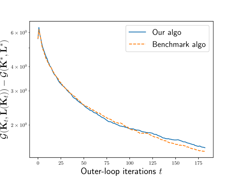
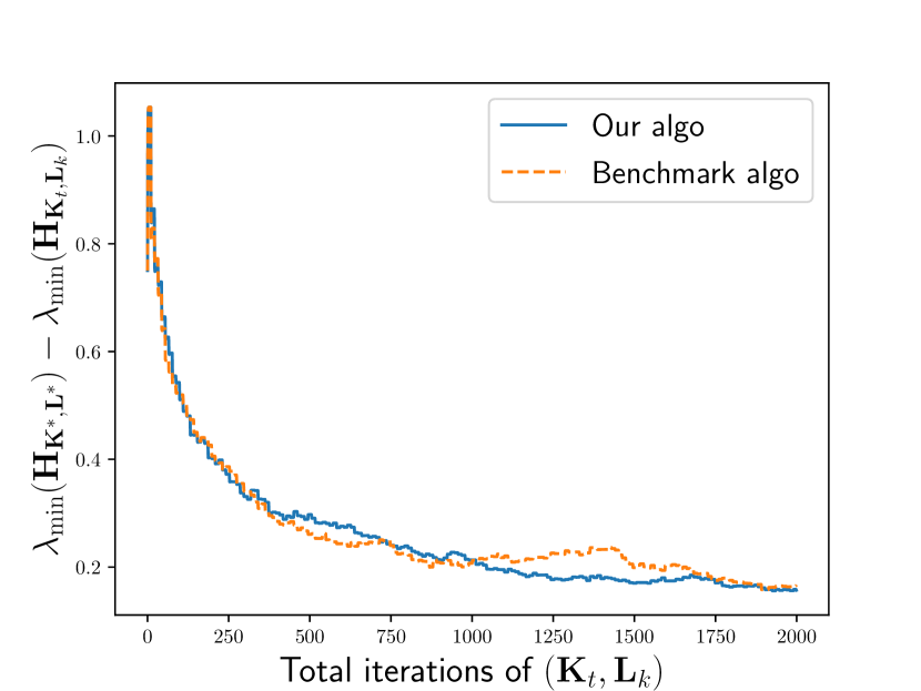
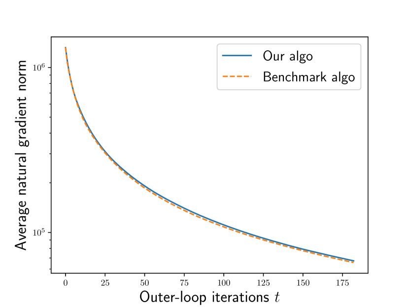
Figure 1: Comparison between Algorithm 2 and the benchmark algorithm when using a fixed number of inner-loop iterations, exact inner-loop natural gradient, and estimated outer-loop natural gradients with $M_{2}=5\times 10^{5}$, $\tau_{1}=0.1$, $\tau_{2}=2\times 10^{-3}$, and $r_{2}=0.02$. In the left, middle, and right figure, we show the convergence in terms of $\mathcal{G}(\boldsymbol{K},\boldsymbol{L})$ (left), $\lambda_{\min}(\boldsymbol{H}_{\boldsymbol{K},\boldsymbol{L}})$ (center), and $T^{-1}\sum_{t=0}^{T-1}\|\boldsymbol{F}_{\boldsymbol{K}_{t},\boldsymbol{L}(\boldsymbol{K}_{t})}\|_{F}^{2}$ (right) respectively.

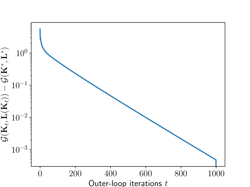
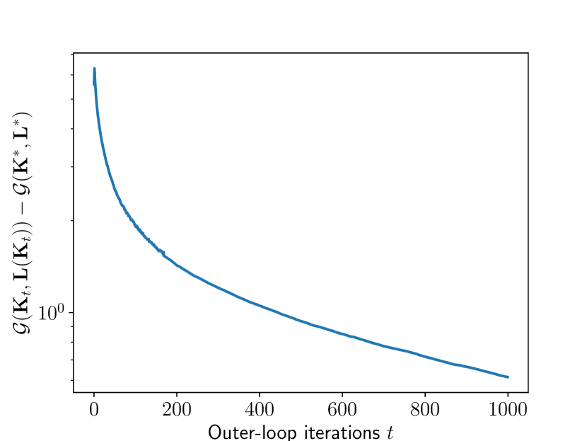
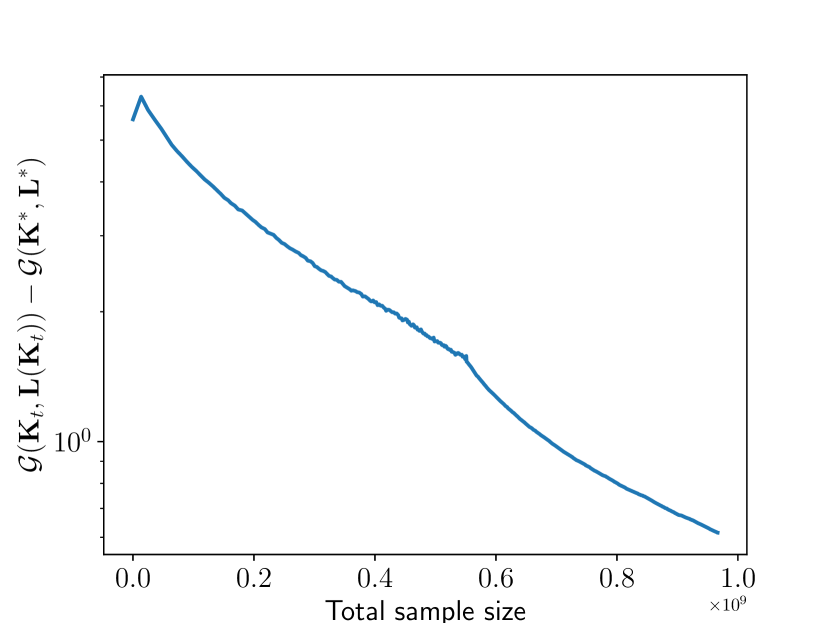
Figure 2: Last-iterate convergence results of Algorithm 2 with $r_{1}=0.5$, $M_{1}=10^{6}$, and $\tau_{1}=0.04$: last-iterate convergence when using exact inner-loop solutions and exact outer-loop natural gradients (left); last-iterate convergence when using estimated inner-loop & outer-loop natural gradients (center); relationship between sample size and last-iterate convergence when using estimated inner-loop & outer-loop natural gradients (right).

7 Conclusion

In this work, we provided a novel global last-iterate convergence result for nested algorithms for zero-sum LQ games in the deterministic setting. Moreover, we showed a $\tilde{\mathcal{O}}(\epsilon^{-2})$ sample complexity for a derivative-free nested natural policy gradient algorithm for solving the zero-sum LQ dynamic game problem, which guarantees last-iterate convergence. Possible future research directions include (a) extending our analysis to continuous-time and infinite-horizon settings beyond our finite-horizon setting using techniques such as sensitivity analysis for stable continuous-time Lyapunov equations [49], (b) improving the dependence on problem dimensions and considering more general noise distributions since the boundedness of noises is not required by the stability constraint under the finite-horizon setting, and (c) designing theoretically grounded single-loop algorithms for zero-sum LQ games.

Complimentary results on structural properties of Zero-sum LQ games, concentration results, and matrix inequalities are presented in Appendix A in preparation for the detailed statements of the main results and their complete proofs in Appendix B. We keep our earlier results on sample complexity improvement for searching stationary NE solution in Appendix C and benchmark algorithm in D.

Appendix A Technical Lemma and Auxiliary Results

A.1 Summary of Notations

Below is a summary of the intensely used notations for convenient lookup.

$$\phi \coloneqq\lambda_{\min}(\boldsymbol{\Sigma}_{0}),$$

$$\boldsymbol{H}_{\boldsymbol{K},\boldsymbol{L}} \coloneqq\boldsymbol{R}^{w}-\boldsymbol{D}^{\top}\boldsymbol{P}_{\boldsymbol{K},\boldsymbol{L}}\boldsymbol{D},$$

$$\boldsymbol{E}_{\boldsymbol{K},\boldsymbol{L}} \coloneqq(-\boldsymbol{R}^{w}+\boldsymbol{D}^{\top}\boldsymbol{P}_{\boldsymbol{K},\boldsymbol{L}}\boldsymbol{D})\boldsymbol{L}-\boldsymbol{D}^{\top}\boldsymbol{P}_{\boldsymbol{K},\boldsymbol{L}}(\boldsymbol{A}-\boldsymbol{BK}),$$

$$\boldsymbol{F}_{\boldsymbol{K},\boldsymbol{L}} \coloneqq(\boldsymbol{R}^{u}+\boldsymbol{B}^{\top}\boldsymbol{P}_{\boldsymbol{K},\boldsymbol{L}}\boldsymbol{B})\boldsymbol{K}-\boldsymbol{B}^{\top}\boldsymbol{P}_{\boldsymbol{K},\boldsymbol{L}}(\boldsymbol{A}-\boldsymbol{DL}),$$

$$\boldsymbol{G}_{\boldsymbol{K},\boldsymbol{L}(\boldsymbol{K})} \coloneqq\boldsymbol{R}^{u}+\boldsymbol{B}^{\top}\widetilde{\boldsymbol{P}}_{\boldsymbol{K},\boldsymbol{L}(\boldsymbol{K})}\boldsymbol{B},$$

$$\widetilde{\boldsymbol{P}}_{\boldsymbol{K},\boldsymbol{L}(\boldsymbol{K})} \coloneqq\boldsymbol{P}_{\boldsymbol{K},\boldsymbol{L}(\boldsymbol{K})}+\boldsymbol{P}_{\boldsymbol{K},\boldsymbol{L}(\boldsymbol{K})}\boldsymbol{D}(\boldsymbol{R}^{w}-\boldsymbol{D}^{\top}\boldsymbol{P}_{\boldsymbol{K},\boldsymbol{L}(\boldsymbol{K})}\boldsymbol{D})^{-1}\boldsymbol{D}^{\top}\boldsymbol{P}_{\boldsymbol{K},\boldsymbol{L}(\boldsymbol{K})},$$

$$\boldsymbol{A}_{\boldsymbol{K},\boldsymbol{L}} \coloneqq\boldsymbol{A}-\boldsymbol{BK}-\boldsymbol{DL},$$

$$\boldsymbol{L}(\boldsymbol{K}) \coloneqq\operatorname*{arg\,max}_{\boldsymbol{L}}\mathcal{G}(\boldsymbol{K},\boldsymbol{L})=(-\boldsymbol{R}^{w}+\boldsymbol{D}^{\top}\boldsymbol{P}_{\boldsymbol{K},\boldsymbol{L}(\boldsymbol{K})}\boldsymbol{D})^{-1}\boldsymbol{D}^{\top}\boldsymbol{P}_{\boldsymbol{K},\boldsymbol{L}(\boldsymbol{K})}(\boldsymbol{A}-\boldsymbol{BK}),$$

$$\Phi(\boldsymbol{K}) \coloneqq\mathcal{G}(\boldsymbol{K},\boldsymbol{L}(\boldsymbol{K})),$$

$$\widetilde{\boldsymbol{F}}_{\boldsymbol{K},\boldsymbol{L}} \coloneqq\frac{1}{2}\widetilde{\nabla}_{\boldsymbol{K}}\mathcal{G}(\boldsymbol{K},\boldsymbol{L})\widetilde{\boldsymbol{\Sigma}}_{\boldsymbol{K},\boldsymbol{L}}^{-1},$$

$$\nabla_{\boldsymbol{K}}\mathcal{G}_{r_{2}}(\boldsymbol{K},\boldsymbol{L}) \coloneqq\mathbb{E}[\widetilde{\nabla}_{\boldsymbol{K}}\mathcal{G}(\boldsymbol{K},\boldsymbol{L})]=\nabla_{\boldsymbol{K}}\mathbb{E}_{\boldsymbol{V}}[\mathcal{G}(\boldsymbol{K}+r_{2}\boldsymbol{V},\boldsymbol{L})],$$

$$\boldsymbol{F}_{\boldsymbol{K},\boldsymbol{L}}^{r} \coloneqq\mathbb{E}[\widetilde{\boldsymbol{F}}_{\boldsymbol{K},\boldsymbol{L}}],$$

$$V(\widetilde{\boldsymbol{F}}_{\boldsymbol{K},\boldsymbol{L}}) \coloneqq(\widetilde{\boldsymbol{F}}_{\boldsymbol{K},\boldsymbol{L}}-\boldsymbol{F}_{\boldsymbol{K},\boldsymbol{L}}^{r})^{\top}(\widetilde{\boldsymbol{F}}_{\boldsymbol{K},\boldsymbol{L}}-\boldsymbol{F}_{\boldsymbol{K},\boldsymbol{L}}^{r}),$$

$$d_{\boldsymbol{\Sigma}} \coloneqq m^{2}(N+1),\quad d_{\boldsymbol{K}}\coloneqq d\,m\,N,\quad d_{\boldsymbol{L}}\coloneqq n\,m\,N,\quad d_{\boldsymbol{P}}\coloneqq m^{2}(N+1),$$

$$\epsilon_{l} \coloneqq\sup_{\boldsymbol{K}\in\hat{\mathcal{K}}}\biggl{\{}\sqrt{\lambda_{\min}^{-1}(\boldsymbol{H}_{\boldsymbol{K},\boldsymbol{L}(\boldsymbol{K})})\cdot\epsilon_{1}}\biggr{\}},$$

$$A_{K_{h},L_{h}} \coloneqq A_{h}-B_{h}K_{h}-D_{h}L_{h},$$

$$\mathcal{R}_{K_{h},K_{h}^{\prime}} \coloneqq(K_{h}^{\prime}-K_{h})^{\top}F_{K_{h},L(K_{h})}+F_{K_{h},L(K_{h})}^{\top}(K_{h}^{\prime}-K_{h})$$

$$\quad+(K_{h}^{\prime}-K_{h})^{\top}(R_{h}^{u}+B_{h}^{\top}\widetilde{P}_{K_{h+1},L(K_{h+1})}B_{h})(K_{h}^{\prime}-K_{h}),$$

$$G_{h} \coloneqq R_{h}^{u}+B_{h}^{\top}\widetilde{P}_{K_{h+1},L(K_{h+1})}B_{h},$$

$$F_{K_{h},L_{h}}^{r} \coloneqq\mathbb{E}[\widetilde{F}_{K_{h},L_{h}}],$$

$$V(\widetilde{F}_{K_{h},L_{h}}) \coloneqq(\widetilde{F}_{K_{h},L_{h}}-F_{K_{h},L_{h}}^{r})^{\top}(\widetilde{F}_{K_{h},L_{h}}-F_{K_{h},L_{h}}^{r}),$$

$$\Xi_{K_{h},K_{h}^{\prime}} \coloneqq-(R_{h}^{w}-D_{h}^{\top}P_{K_{h+1},L(K_{h+1})}D_{h})L(K_{h}^{\prime})-D_{h}^{\top}P_{K_{h+1},L(K_{h+1})}(A_{h}-B_{h}K_{h}^{\prime}),$$

$$E_{K_{h},L_{h}} \coloneqq(-R_{h}^{w}+D_{h}^{\top}P_{K_{h+1},L_{h+1}}D_{h})L_{h}-D_{h}^{\top}P_{K_{h+1},L_{h+1}}(A_{h}-B_{h}K_{h}),$$

$$F_{K_{h},L_{h}} \coloneqq(R_{h}^{u}+B_{h}^{\top}P_{K_{h+1},L_{h+1}}B_{h})K_{h}-B_{h}^{\top}P_{K_{h+1},L_{h+1}}(A_{h}-D_{h}L_{h}),$$

$$F_{K_{h},L(K_{h})} \coloneqq(R_{h}^{u}+B_{h}^{\top}\widetilde{P}_{K_{h+1},L(K_{h+1})}B_{h})K_{h}-B_{h}^{\top}\tilde{P}_{K_{h+1},L(K_{h+1})}A_{h},$$

$$\widetilde{P}_{K_{h+1},L(K_{h+1})} \coloneqq P_{K_{h+1},L(K_{h+1})}+P_{K_{h+1},L(K_{h+1})}D_{h}(R_{h}^{w}-D_{h}^{\top}P_{K_{h+1},L(K_{h+1})}D_{h})^{-1}D_{h}^{\top}P_{K_{h+1},L(K_{h+1})}$$

where horizon index $h=0,\cdots,N-1$. Assumption 1 ensures that $\boldsymbol{\Sigma}_{0}\succ 0$ and hence $\phi>0$. Let $\boldsymbol{K}_{0}\in\mathcal{K}$ and recall

$$\hat{\mathcal{K}} \coloneqq\biggl{\{}\boldsymbol{K}\mid\eqref{eq:riccati}\text{ admits a solution $\boldsymbol{P}_{\boldsymbol{K},\boldsymbol{L}(\boldsymbol{K})}\succeq 0$ and $\boldsymbol{P}_{\boldsymbol{K},\boldsymbol{L}(\boldsymbol{K})}\preceq\boldsymbol{P}_{\boldsymbol{K}_{0},\boldsymbol{L}(\boldsymbol{K}_{0})}+\frac{\lambda_{\min}(\boldsymbol{H}_{\boldsymbol{K}_{0},\boldsymbol{L}(\boldsymbol{K}_{0})})}{2\|\boldsymbol{D}\|}\cdot\boldsymbol{I}$}\biggr{\}},$$

$$\hat{\mathcal{L}} \coloneqq\Bigl{\{}\boldsymbol{L}\in\mathcal{S}_{2}\mid\|\boldsymbol{L}(\boldsymbol{K})-\boldsymbol{L}\|_{F}\leq H,\,\boldsymbol{K}\in\hat{\mathcal{K}}\Bigr{\}},$$

where $H\coloneqq\sup_{\boldsymbol{K}\in\hat{\mathcal{K}}}\lambda_{\min}^{-1}(\boldsymbol{H}_{\boldsymbol{K},\boldsymbol{L}(\boldsymbol{K})})$ and $\boldsymbol{K}_{0}\in\mathcal{K}$. For any $(\boldsymbol{K},\boldsymbol{L})\in\hat{\mathcal{K}}\times\hat{\mathcal{L}}$, the following amounts are positive and well-defined because of the boundedness of $\hat{\mathcal{K}}$, $\hat{\mathcal{L}}$.

$$D_{1} \coloneqq\inf_{(\boldsymbol{K},\boldsymbol{L})\in\hat{\mathcal{K}}\times\hat{\mathcal{L}}}\min\biggl{\{}1,\frac{\phi}{2\operatorname{Tr}(\boldsymbol{\Sigma}_{\boldsymbol{K},\boldsymbol{L}})\|\boldsymbol{B}\|(2\|\boldsymbol{A}_{\boldsymbol{K},\boldsymbol{L}}\|+\|\boldsymbol{B}\|)}\biggr{\}},$$

$$D_{2} \coloneqq\inf_{(\boldsymbol{K},\boldsymbol{L})\in\hat{\mathcal{K}}\times\hat{\mathcal{L}}}\min\biggl{\{}1,\frac{\phi}{2\operatorname{Tr}(\boldsymbol{\Sigma}_{\boldsymbol{K},\boldsymbol{L}})\|\boldsymbol{D}\|(2\|\boldsymbol{A}_{\boldsymbol{K},\boldsymbol{L}}\|+\|\boldsymbol{D}\|)}\biggr{\}},$$

$$D_{3} \coloneqq\inf_{(\boldsymbol{K},\boldsymbol{L})\in\hat{\mathcal{K}}\times\hat{\mathcal{L}}}\min\biggl{\{}1,H^{-1},H^{-1}\biggl{(}\frac{\phi}{2\operatorname{Tr}(\boldsymbol{\Sigma}_{\boldsymbol{K},\boldsymbol{L}})\|\boldsymbol{D}\|(2\|\boldsymbol{A}_{\boldsymbol{K},\boldsymbol{L}}\|+\|\boldsymbol{D}\|)}\biggr{)}^{2}\biggr{\}}.$$

A.2 Structural Properties of Zero-sum LQ Games

This section summarizes basic results for LQ games, some of which are similar to results in [5], [33], and [1]. The following results will be used Appendix B. Recall the shorthand notations $\Delta_{\boldsymbol{K}}\coloneqq\boldsymbol{K}^{\prime}-\boldsymbol{K}$ for $\boldsymbol{K}^{\prime},\boldsymbol{K}\in\mathcal{K}$.

Lemma 5.

(Lemma B.9 in [1]) For any $\boldsymbol{K}\in\mathcal{K}$, there exists some $\mathcal{B}_{2,\boldsymbol{K}}>0$ such that all $\boldsymbol{K}^{\prime}$ satisfying $\|\boldsymbol{K}^{\prime}-\boldsymbol{K}\|_{F}\leq\mathcal{B}_{2,\boldsymbol{K}}$ satisfy $\boldsymbol{K}^{\prime}\in\mathcal{K}$. Then for any $\boldsymbol{K}\in\hat{\mathcal{K}}$ with $\boldsymbol{K}_{0}\in\mathcal{K}$, there exists a positive constant $B_{2}$ such that all $\boldsymbol{K}^{\prime}$ satisfying $\|\boldsymbol{K}^{\prime}-\boldsymbol{K}\|_{F}\leq B_{2}$ satisfy $\boldsymbol{K}^{\prime}\in\mathcal{K}$.

Lemma 6.

(Lemma B.7 in [1]: Local Lipschitz continuity of $\boldsymbol{\Sigma}_{\boldsymbol{K},\boldsymbol{L}(\boldsymbol{K})}$ ) For any $\boldsymbol{K},\boldsymbol{K}^{\prime}\in\mathcal{K}$, there exist some $\mathcal{B}_{1,\boldsymbol{K}}$, $\mathcal{B}_{\boldsymbol{\Sigma},\boldsymbol{K}}>0$ that are continuous functions of $\boldsymbol{K}$ such that all $\boldsymbol{K}^{\prime}$ satisfying $\|\boldsymbol{K}^{\prime}-\boldsymbol{K}\|_{F}\leq\mathcal{B}_{1,\boldsymbol{K}}$ satisfy

$$\|\boldsymbol{\Sigma}_{\boldsymbol{K}^{\prime},\boldsymbol{L}(\boldsymbol{K}^{\prime})}-\boldsymbol{\Sigma}_{\boldsymbol{K},\boldsymbol{L}(\boldsymbol{K})}\|_{F} \leq\mathcal{B}_{\boldsymbol{\Sigma},\boldsymbol{K}}\cdot\|\boldsymbol{K}^{\prime}-\boldsymbol{K}\|_{F}.$$

For convenience, we define the following positive constants

$$B_{1}\coloneqq\inf_{\boldsymbol{K}\in\hat{\mathcal{K}}}\mathcal{B}_{1,\boldsymbol{K}},\quad B_{\boldsymbol{\Sigma}}\coloneqq\sup_{\boldsymbol{K}\in\hat{\mathcal{K}}}\mathcal{B}_{\boldsymbol{\Sigma},\boldsymbol{K}}.$$

We define some shorthands that will be frequently used hereafter: $\Delta_{\boldsymbol{K}}\coloneqq\boldsymbol{K}^{\prime}-\boldsymbol{K}$ and $\Delta_{\boldsymbol{L}}\coloneqq\boldsymbol{L}^{\prime}-\boldsymbol{L}$.

Lemma 7.

(Local Lipschitz continuity of $P_{K,L}$) Let $\boldsymbol{K}_{0}\in\mathcal{K}$ and consider the corresponding set $\hat{\mathcal{K}},\hat{\mathcal{L}}$ as defined in (14),(16). For any $(\boldsymbol{K},\boldsymbol{L})\in\hat{\mathcal{K}}\times\hat{\mathcal{L}}$ with structures defined in (4) and $(\boldsymbol{K}^{\prime}\in\mathcal{K},\boldsymbol{L}^{\prime})$ that satisfy

$$\|\boldsymbol{K}^{\prime}-\boldsymbol{K}\| \leq D_{1},\quad\|\boldsymbol{L}^{\prime}-\boldsymbol{L}\|\leq D_{2}.$$

Then there exist positive constants $l_{5}$, $l_{6}$ such that

$$\|\boldsymbol{P}_{\boldsymbol{K}^{\prime},\boldsymbol{L}}-\boldsymbol{P}_{\boldsymbol{K},\boldsymbol{L}}\|\leq l_{5}\|\boldsymbol{K}^{\prime}-\boldsymbol{K}\|, \quad\|\boldsymbol{P}_{\boldsymbol{K},\boldsymbol{L}^{\prime}}-\boldsymbol{P}_{\boldsymbol{K},\boldsymbol{L}}\|\leq l_{6}\|\boldsymbol{L}^{\prime}-\boldsymbol{L}\|,$$

where

$$l_{5} \coloneqq\sup_{(\boldsymbol{K},\boldsymbol{L})\in\hat{\mathcal{K}}\times\hat{\mathcal{L}}}2\operatorname{Tr}(\boldsymbol{\Sigma}_{\boldsymbol{K},\boldsymbol{L}})/\phi\cdot((\|\boldsymbol{K}\|+1)\|\boldsymbol{R}^{u}\|+\|\boldsymbol{R}^{u}\|\|\boldsymbol{K}\|+\|\boldsymbol{B}\|(2\|\boldsymbol{A}_{\boldsymbol{K},\boldsymbol{L}}\|+\|\boldsymbol{B}\|)\|\boldsymbol{P}_{\boldsymbol{K},\boldsymbol{L}}\|),$$

$$l_{6} \coloneqq\sup_{(\boldsymbol{K},\boldsymbol{L})\in\hat{\mathcal{K}}\times\hat{\mathcal{L}}}2\operatorname{Tr}(\boldsymbol{\Sigma}_{\boldsymbol{K},\boldsymbol{L}})/\phi\cdot((\|\boldsymbol{L}\|+1)\|\boldsymbol{R}^{v}\|+\|\boldsymbol{R}^{v}\|\|\boldsymbol{L}\|+\|\boldsymbol{D}\|(2\|\boldsymbol{A}_{\boldsymbol{K},\boldsymbol{L}}\|+\|\boldsymbol{D}\|)\|\boldsymbol{P}_{\boldsymbol{K},\boldsymbol{L}}\|).$$

Proof.

We apply Lemma 17 and sensitivity analysis in Lemma 21 with $F=\boldsymbol{A}_{\boldsymbol{K}^{\prime},\boldsymbol{L}}$, $M=\boldsymbol{Q}+(\boldsymbol{K}^{\prime})^{\top}\boldsymbol{R}^{u}(\boldsymbol{K}^{\prime})-\boldsymbol{L}^{\top}\boldsymbol{R}^{v}\boldsymbol{L}$, $\boldsymbol{H}$ being the solution of the Lyapunov equation: $I+\boldsymbol{A}_{\boldsymbol{K},\boldsymbol{L}}^{\top}\boldsymbol{H}\boldsymbol{A}_{\boldsymbol{K},\boldsymbol{L}}=\boldsymbol{H}$ and $X=\boldsymbol{P}_{\boldsymbol{K}^{\prime},\boldsymbol{L}}$. Then if $\|\boldsymbol{H}\|\|\boldsymbol{B}\Delta_{\boldsymbol{K}}\|(2\|\boldsymbol{A}_{\boldsymbol{K},\boldsymbol{L}}\|+\|\boldsymbol{B}\Delta_{\boldsymbol{K}}\|)<1$, we have

$$\|\boldsymbol{P}_{\boldsymbol{K}^{\prime},\boldsymbol{L}}-\boldsymbol{P}_{\boldsymbol{K},\boldsymbol{L}}\| \leq(1-\|\boldsymbol{H}\|\|\boldsymbol{B}\Delta_{\boldsymbol{K}}\|(2\|\boldsymbol{A}_{\boldsymbol{K},\boldsymbol{L}}\|+\|\boldsymbol{B}\Delta_{\boldsymbol{K}}\|))^{-1}\|\boldsymbol{H}\|$$

$$\quad\cdot(\|(\boldsymbol{K}^{\prime})^{\top}\boldsymbol{R}^{u}\Delta_{\boldsymbol{K}}+\Delta_{\boldsymbol{K}}^{\top}\boldsymbol{R}^{u}\boldsymbol{K}\|+\|\boldsymbol{B}\Delta_{\boldsymbol{K}}\|(2\|\boldsymbol{A}_{\boldsymbol{K},\boldsymbol{L}}\|+\|\boldsymbol{B}\Delta_{\boldsymbol{K}}\|)\|\boldsymbol{P}_{\boldsymbol{K},\boldsymbol{L}}\|)$$

$$\leq(1-\|\boldsymbol{H}\|\|\boldsymbol{B}\Delta_{\boldsymbol{K}}\|(2\|\boldsymbol{A}_{\boldsymbol{K},\boldsymbol{L}}\|+\|\boldsymbol{B}\Delta_{\boldsymbol{K}}\|))^{-1}\|\boldsymbol{H}\|\cdot((\|\boldsymbol{K}\|+\|\Delta_{\boldsymbol{K}}\|)\|\boldsymbol{R}^{u}\|$$

$$\quad+\|\boldsymbol{R}^{u}\|\|\boldsymbol{K}\|+\|\boldsymbol{B}\|(2\|\boldsymbol{A}_{\boldsymbol{K},\boldsymbol{L}}\|+\|\boldsymbol{B}\|\|\Delta_{\boldsymbol{K}}\|)\|\boldsymbol{P}_{\boldsymbol{K},\boldsymbol{L}}\|)\cdot\|\Delta_{\boldsymbol{K}}\|.$$

When we apply Lemma 20 to bound $\|\boldsymbol{H}\|$ and choose $\boldsymbol{K}^{\prime}$ such that $\|\Delta_{\boldsymbol{K}}\|\leq D_{1}$, then

$$\|\boldsymbol{H}\|\|\boldsymbol{B}\Delta_{\boldsymbol{K}}\|(2\|\boldsymbol{A}_{\boldsymbol{K},\boldsymbol{L}}\|+\|\boldsymbol{B}\Delta_{\boldsymbol{K}}\|) \leq\|\boldsymbol{H}\|\|\boldsymbol{B}\|\|\Delta_{\boldsymbol{K}}\|(2\|\boldsymbol{A}_{\boldsymbol{K},\boldsymbol{L}}\|+\|\boldsymbol{B}\|\|\Delta_{\boldsymbol{K}}\|)<1.$$

We can then ensure that

$$\|\boldsymbol{P}_{\boldsymbol{K}^{\prime},\boldsymbol{L}}-\boldsymbol{P}_{\boldsymbol{K},\boldsymbol{L}}\| \leq 2\operatorname{Tr}(\boldsymbol{\Sigma}_{\boldsymbol{K},\boldsymbol{L}})/\phi\cdot((\|\boldsymbol{K}\|+1)\|\boldsymbol{R}^{u}\|+\|\boldsymbol{R}^{u}\|\|\boldsymbol{K}\|+\|\boldsymbol{B}\|(2\|\boldsymbol{A}_{\boldsymbol{K},\boldsymbol{L}}\|+\|\boldsymbol{B}\|)\|\boldsymbol{P}_{\boldsymbol{K},\boldsymbol{L}}\|)\cdot\|\Delta_{\boldsymbol{K}}\|.$$

For $\boldsymbol{L}^{\prime}$ and $\boldsymbol{L}$, the proof is similar and hence omitted

$$\|\boldsymbol{P}_{\boldsymbol{K},\boldsymbol{L}^{\prime}}-\boldsymbol{P}_{\boldsymbol{K},\boldsymbol{L}}\| \leq 2\operatorname{Tr}(\boldsymbol{\Sigma}_{\boldsymbol{K},\boldsymbol{L}})/\phi\cdot((\|\boldsymbol{L}\|+1)\|\boldsymbol{R}^{v}\|+\|\boldsymbol{R}^{v}\|\|\boldsymbol{L}\|+\|\boldsymbol{D}\|(2\|\boldsymbol{A}_{\boldsymbol{K},\boldsymbol{L}}\|+\|\boldsymbol{D}\|)\|\boldsymbol{P}_{\boldsymbol{K},\boldsymbol{L}}\|)\cdot\|\Delta_{\boldsymbol{L}}\|,$$

when $\|\Delta_{\boldsymbol{L}}\|\leq D_{2}$. The proof is concluded by simply applying the definitions of $l_{5}$, $l_{6}$. ∎

Lemma 8.

(Lipschitz continuity of $\boldsymbol{E}_{\boldsymbol{K},\boldsymbol{L}},\boldsymbol{F}_{\boldsymbol{K},\boldsymbol{L}}$) Let $\boldsymbol{K}_{0}\in\mathcal{K}$ and consider the corresponding sets $\hat{\mathcal{K}}$, $\hat{\mathcal{L}}$ as defined in (14), (16). For any $(\boldsymbol{K},\boldsymbol{L})\in\hat{\mathcal{K}}\times\hat{\mathcal{L}}$ and $(\boldsymbol{K}^{\prime}\in\mathcal{K},\boldsymbol{L}^{\prime})$ with structures defined in (4) that satisfy

$$\|\boldsymbol{K}^{\prime}-\boldsymbol{K}\| \leq D_{1},\quad\|\boldsymbol{L}^{\prime}-\boldsymbol{L}\|\leq D_{2},$$

There exist positive constants $l_{1}$, $l_{2}$, $l_{3}$, and $l_{4}$ such that

$$\|\boldsymbol{F}_{\boldsymbol{K}^{\prime},\boldsymbol{L}}-\boldsymbol{F}_{\boldsymbol{K},\boldsymbol{L}}\| \leq l_{1}\|\boldsymbol{K}^{\prime}-\boldsymbol{K}\|,\quad\|\boldsymbol{F}_{\boldsymbol{K},\boldsymbol{L}^{\prime}}-\boldsymbol{F}_{\boldsymbol{K},\boldsymbol{L}}\|\leq l_{2}\|\boldsymbol{L}^{\prime}-\boldsymbol{L}\|,$$

$$\|\boldsymbol{E}_{\boldsymbol{K}^{\prime},\boldsymbol{L}}-\boldsymbol{E}_{\boldsymbol{K},\boldsymbol{L}}\| \leq l_{3}\|\boldsymbol{K}^{\prime}-\boldsymbol{K}\|,\quad\|\boldsymbol{E}_{\boldsymbol{K},\boldsymbol{L}^{\prime}}-\boldsymbol{E}_{\boldsymbol{K},\boldsymbol{L}}\|\leq l_{4}\|\boldsymbol{L}^{\prime}-\boldsymbol{L}\|,$$

where

$$l_{1} \coloneqq\sup_{(\boldsymbol{K},\boldsymbol{L})\in\hat{\mathcal{K}}\times\hat{\mathcal{L}}}l_{5}\|\boldsymbol{B}\|(\|\boldsymbol{A}_{\boldsymbol{K},\boldsymbol{L}}\|+\|\boldsymbol{B}\|)+\|\boldsymbol{R}^{u}\|+\|\boldsymbol{B}\|^{2}\|\boldsymbol{P}_{\boldsymbol{K},\boldsymbol{L}}\|$$

$$l_{2} \coloneqq\sup_{(\boldsymbol{K},\boldsymbol{L})\in\hat{\mathcal{K}}\times\hat{\mathcal{L}}}l_{6}\|\boldsymbol{B}\|(\|\boldsymbol{A}_{\boldsymbol{K},\boldsymbol{L}}\|+\|\boldsymbol{D}\|)+\|\boldsymbol{B}\|\|\boldsymbol{P}_{\boldsymbol{K},\boldsymbol{L}}\|\|\boldsymbol{D}\|$$

$$l_{3} \coloneqq\sup_{(\boldsymbol{K},\boldsymbol{L})\in\hat{\mathcal{K}}\times\hat{\mathcal{L}}}l_{5}\|\boldsymbol{D}\|(\|\boldsymbol{A}_{\boldsymbol{K},\boldsymbol{L}}\|+\|\boldsymbol{B}\|)+\|\boldsymbol{D}\|\|\boldsymbol{P}_{\boldsymbol{K},\boldsymbol{L}}\|\|\boldsymbol{B}\|$$

$$l_{4} \coloneqq\sup_{(\boldsymbol{K},\boldsymbol{L})\in\hat{\mathcal{K}}\times\hat{\mathcal{L}}}l_{6}\|\boldsymbol{D}\|(\|\boldsymbol{A}_{\boldsymbol{K},\boldsymbol{L}}\|+\|\boldsymbol{D}\|)+\|\boldsymbol{R}^{w}\|+\|\boldsymbol{D}\|^{2}\|\boldsymbol{P}_{\boldsymbol{K},\boldsymbol{L}}\|$$

Proof.

We start from the explicit expression of $\boldsymbol{E}_{\boldsymbol{K},\boldsymbol{L}}$ and $\boldsymbol{F}_{\boldsymbol{K},\boldsymbol{L}}$

$$\|\boldsymbol{F}_{\boldsymbol{K}^{\prime},\boldsymbol{L}}-\boldsymbol{F}_{\boldsymbol{K},\boldsymbol{L}}\| =\|\boldsymbol{B}^{\top}(\boldsymbol{P}_{\boldsymbol{K}^{\prime},\boldsymbol{L}}-\boldsymbol{P}_{\boldsymbol{K},\boldsymbol{L}})(\boldsymbol{BK}^{\prime}+\boldsymbol{DL}-\boldsymbol{A})+(\boldsymbol{R}^{u}+\boldsymbol{B}^{\top}\boldsymbol{P}_{\boldsymbol{K},\boldsymbol{L}}\boldsymbol{B})(\boldsymbol{K}^{\prime}-\boldsymbol{K})\|$$

$$\leq\left(\|\boldsymbol{B}\|l_{5}(\|\boldsymbol{A}_{\boldsymbol{K},\boldsymbol{L}}\|+\|\boldsymbol{B}\|)+\|\boldsymbol{R}^{u}\|+\|\boldsymbol{B}\|^{2}\|\boldsymbol{P}_{\boldsymbol{K},\boldsymbol{L}}\|\right)\cdot\|\boldsymbol{K}^{\prime}-\boldsymbol{K}\|\leq l_{1}\|\boldsymbol{K}^{\prime}-\boldsymbol{K}\|,$$

where the first inequality follows from Lemma 7 with $\|\Delta_{\boldsymbol{K}}\|\leq D_{1}$. Following the same proof spirit, we have

$$\|\boldsymbol{F}_{\boldsymbol{K},\boldsymbol{L}^{\prime}}-\boldsymbol{F}_{\boldsymbol{K},\boldsymbol{L}}\| =\|-\boldsymbol{B}^{\top}(\boldsymbol{P}_{\boldsymbol{K},\boldsymbol{L}^{\prime}}-\boldsymbol{P}_{\boldsymbol{K},\boldsymbol{L}})\boldsymbol{A}_{\boldsymbol{K},\boldsymbol{L}^{\prime}}+\boldsymbol{B}^{\top}\boldsymbol{P}_{\boldsymbol{K},\boldsymbol{L}}\boldsymbol{D}(\boldsymbol{L}^{\prime}-\boldsymbol{L})\|$$

$$\leq\left(l_{6}\|\boldsymbol{B}\|(\|\boldsymbol{A}_{\boldsymbol{K},\boldsymbol{L}}\|+\|\boldsymbol{D}\|)+\|\boldsymbol{B}\|\|\boldsymbol{P}_{\boldsymbol{K},\boldsymbol{L}}\|\|\boldsymbol{D}\|\right)\cdot\|\boldsymbol{L}^{\prime}-\boldsymbol{L}\|,$$

$$\|\boldsymbol{E}_{\boldsymbol{K}^{\prime},\boldsymbol{L}}-\boldsymbol{E}_{\boldsymbol{K},\boldsymbol{L}}\| =-\boldsymbol{D}^{\top}(\boldsymbol{P}_{\boldsymbol{K}^{\prime},\boldsymbol{L}}-\boldsymbol{P}_{\boldsymbol{K},\boldsymbol{L}})\boldsymbol{A}_{\boldsymbol{K}^{\prime},\boldsymbol{L}}+\boldsymbol{D}^{\top}\boldsymbol{P}_{\boldsymbol{K},\boldsymbol{L}}\boldsymbol{B}(\boldsymbol{K}^{\prime}-\boldsymbol{K})$$

$$\leq\left(l_{5}\|\boldsymbol{D}\|(\|\boldsymbol{A}_{\boldsymbol{K},\boldsymbol{L}}\|+\|\boldsymbol{B}\|)+\|\boldsymbol{D}\|\|\boldsymbol{P}_{\boldsymbol{K},\boldsymbol{L}}\|\|\boldsymbol{B}\|\right)\cdot\|\boldsymbol{K}^{\prime}-\boldsymbol{K}\|,$$

$$\|\boldsymbol{E}_{\boldsymbol{K},\boldsymbol{L}^{\prime}}-\boldsymbol{E}_{\boldsymbol{K},\boldsymbol{L}}\| =\|-\boldsymbol{D}^{\top}(\boldsymbol{P}_{\boldsymbol{K},\boldsymbol{L}^{\prime}}-\boldsymbol{P}_{\boldsymbol{K},\boldsymbol{L}})\boldsymbol{A}_{\boldsymbol{K},\boldsymbol{L}^{\prime}}+(-\boldsymbol{R}^{w}+\boldsymbol{D}^{\top}\boldsymbol{P}_{\boldsymbol{K},\boldsymbol{L}}\boldsymbol{D})(\boldsymbol{L}^{\prime}-\boldsymbol{L})\|$$

$$\leq\left(l_{6}\|\boldsymbol{D}\|(\|\boldsymbol{A}_{\boldsymbol{K},\boldsymbol{L}}\|+\|\boldsymbol{D}\|)+\|\boldsymbol{R}^{w}\|+\|\boldsymbol{D}\|^{2}\|\boldsymbol{P}_{\boldsymbol{K},\boldsymbol{L}}\|\right)\cdot\|\boldsymbol{L}^{\prime}-\boldsymbol{L}\|,$$

when we also require $\|\Delta_{\boldsymbol{L}}\|\leq D_{2}$. We conclude the proof by applying the definitions of $l_{1},l_{2},l_{3},l_{4}$. ∎

Lemma 9.

(Local Lipschitz continuity of $\boldsymbol{\Sigma}_{\boldsymbol{K},\boldsymbol{L}}$) Let $\boldsymbol{K}_{0}\in\mathcal{K}$ and consider the corresponding sets $\hat{\mathcal{K}}$, $\hat{\mathcal{L}}$ as defined in (14), (16). For any $(\boldsymbol{K},\boldsymbol{L})\in\hat{\mathcal{K}}\times\hat{\mathcal{L}}$ and $(\boldsymbol{K}^{\prime}\in\mathcal{K},\boldsymbol{L}^{\prime})$ with structures defined in (4) that satisfy

$$\|\boldsymbol{K}^{\prime}-\boldsymbol{K}\| \leq D_{1},\quad\|\boldsymbol{L}^{\prime}-\boldsymbol{L}\|\leq D_{2},$$

there exist positive constants $l_{7},l_{8}$ such that

$$\|\boldsymbol{\Sigma}_{\boldsymbol{K}^{\prime},\boldsymbol{L}}-\boldsymbol{\Sigma}_{\boldsymbol{K},\boldsymbol{L}}\| \leq l_{7}\|\boldsymbol{K}^{\prime}-\boldsymbol{K}\|,\quad\|\boldsymbol{\Sigma}_{\boldsymbol{K},\boldsymbol{L}^{\prime}}-\boldsymbol{\Sigma}_{\boldsymbol{K},\boldsymbol{L}}\|\leq l_{8}\|\boldsymbol{L}^{\prime}-\boldsymbol{L}\|,$$

where

$$l_{7} \coloneqq\sup_{(\boldsymbol{K},\boldsymbol{L})\in\hat{\mathcal{K}}\times\hat{\mathcal{L}}}2\operatorname{Tr}(\boldsymbol{\Sigma}_{\boldsymbol{K},\boldsymbol{L}})/\phi\cdot\|\boldsymbol{B}\|(2\|\boldsymbol{\Sigma}_{\boldsymbol{K},\boldsymbol{L}}\|+\|\boldsymbol{B}\|)\|\boldsymbol{\Sigma}_{\boldsymbol{K},\boldsymbol{L}}\|,$$

$$l_{8} \coloneqq\sup_{(\boldsymbol{K},\boldsymbol{L})\in\hat{\mathcal{K}}\times\hat{\mathcal{L}}}2\operatorname{Tr}(\boldsymbol{\Sigma}_{\boldsymbol{K},\boldsymbol{L}})/\phi\cdot\|\boldsymbol{D}\|(2\|\boldsymbol{\Sigma}_{\boldsymbol{K},\boldsymbol{L}}\|+\|\boldsymbol{D}\|)\|\boldsymbol{\Sigma}_{\boldsymbol{K},\boldsymbol{L}}\|.$$

Proof.

Here we apply Lemma 17 and Lemma 21 with $F=\boldsymbol{A}_{\boldsymbol{K},\boldsymbol{L}}^{\top}$, $M=\boldsymbol{\Sigma}_{0}$, $X=\boldsymbol{\Sigma}_{\boldsymbol{K},\boldsymbol{L}}$, and $\boldsymbol{H}$ being the solution of the Lyapunov equation $I+\boldsymbol{A}_{\boldsymbol{K},\boldsymbol{L}}\boldsymbol{H}\boldsymbol{A}_{\boldsymbol{K},\boldsymbol{L}}^{\top}=\boldsymbol{H}$. Then if $\|\boldsymbol{H}\|\|\boldsymbol{B}\Delta_{\boldsymbol{K}}\|(2\|\boldsymbol{A}_{\boldsymbol{K},\boldsymbol{L}}\|+2\|\boldsymbol{B}\Delta_{\boldsymbol{K}}\|)<1$, we have

$$\|\boldsymbol{\Sigma}_{\boldsymbol{K}^{\prime},\boldsymbol{L}}-\boldsymbol{\Sigma}_{\boldsymbol{K},\boldsymbol{L}}\| \leq(1-\|\boldsymbol{H}\|\|\boldsymbol{B}\Delta_{\boldsymbol{K}}\|(2\|\boldsymbol{\Sigma}_{\boldsymbol{K},\boldsymbol{L}}\|+\|\boldsymbol{B}\Delta_{\boldsymbol{K}}\|))^{-1}\cdot\|\boldsymbol{H}\|\|\boldsymbol{B}\Delta_{\boldsymbol{K}}\|(2\|\boldsymbol{\Sigma}_{\boldsymbol{K},\boldsymbol{L}}\|+\|\boldsymbol{B}\Delta_{\boldsymbol{K}}\|)\|\boldsymbol{\Sigma}_{\boldsymbol{K},\boldsymbol{L}}\|.$$

We apply Lemma 20 and choose $\boldsymbol{K}^{\prime}$ such that

$$\|\boldsymbol{H}\|\|\boldsymbol{B}\Delta_{\boldsymbol{K}}\|(2\|\boldsymbol{\Sigma}_{\boldsymbol{K},\boldsymbol{L}}\|+2\|\boldsymbol{B}\Delta_{\boldsymbol{K}}\|) \leq\|\boldsymbol{H}\|\|\boldsymbol{B}\|\|\Delta_{\boldsymbol{K}}\|(2\|\boldsymbol{\Sigma}_{\boldsymbol{K},\boldsymbol{L}}\|+2\|\boldsymbol{B}\|\|\Delta_{\boldsymbol{K}}\|)<1,$$

then we have $\|\boldsymbol{\Sigma}_{\boldsymbol{K}^{\prime},\boldsymbol{L}}-\boldsymbol{\Sigma}_{\boldsymbol{K},\boldsymbol{L}}\|\leq 2\operatorname{Tr}(\boldsymbol{\Sigma}_{\boldsymbol{K},\boldsymbol{L}})/\phi\cdot\|\boldsymbol{B}\|(2\|\boldsymbol{\Sigma}_{\boldsymbol{K},\boldsymbol{L}}\|+\|\boldsymbol{B}\|)\|\boldsymbol{\Sigma}_{\boldsymbol{K},\boldsymbol{L}}\|\|\Delta_{\boldsymbol{K}}\|$. Similarly, when $\|\Delta_{\boldsymbol{L}}\|\leq D_{2}$, we have $\|\boldsymbol{\Sigma}_{\boldsymbol{K},\boldsymbol{L}^{\prime}}-\boldsymbol{\Sigma}_{\boldsymbol{K},\boldsymbol{L}}\|\leq 2\operatorname{Tr}(\boldsymbol{\Sigma}_{\boldsymbol{K},\boldsymbol{L}})/\phi\cdot\|\boldsymbol{D}\|(2\|\boldsymbol{\Sigma}_{\boldsymbol{K},\boldsymbol{L}}\|+\|\boldsymbol{D}\|)\|\boldsymbol{\Sigma}_{\boldsymbol{K},\boldsymbol{L}}\|\|\Delta_{\boldsymbol{L}}\|$. Then proof is concluded by applying definitions of $l_{7},l_{8}$. ∎

The following lemma is important for controlling the estimation bias caused by using ZO estimation.

Lemma 10.

(Local Lipschitz continuity of $\nabla_{\boldsymbol{K}}\mathcal{G}(\boldsymbol{K},\boldsymbol{L}),\nabla_{\boldsymbol{L}}\mathcal{G}(\boldsymbol{K},\boldsymbol{L})$) Let $\boldsymbol{K}_{0}\in\mathcal{K}$ and consider corresponding sets $\hat{\mathcal{K}},\hat{\mathcal{L}}$ as defined in (14), (16). For any $(\boldsymbol{K},\boldsymbol{L})\in\hat{\mathcal{K}}\times\hat{\mathcal{L}}$ and $(\boldsymbol{K}^{\prime}\in\mathcal{K},\boldsymbol{L}^{\prime})$ with structures defined in (4) that satisfy

$$\|\boldsymbol{K}^{\prime}-\boldsymbol{K}\| \leq D_{1},\quad\|\boldsymbol{L}^{\prime}-\boldsymbol{L}\|\leq D_{2},$$

then the following inequalities hold

$$\|\nabla_{\boldsymbol{K}}\mathcal{G}(\boldsymbol{K}^{\prime},\boldsymbol{L})-\nabla_{\boldsymbol{K}}\mathcal{G}(\boldsymbol{K},\boldsymbol{L})\|\leq (2l_{1}\|\boldsymbol{\Sigma}_{\boldsymbol{K},\boldsymbol{L}}\|+2l_{1}\cdot l_{7}+2l_{8}\|\boldsymbol{F}_{\boldsymbol{K},\boldsymbol{L}}\|)\|\boldsymbol{K}^{\prime}-\boldsymbol{K}\|$$

$$\|\nabla_{\boldsymbol{K}}\mathcal{G}(\boldsymbol{K},\boldsymbol{L}^{\prime})-\nabla_{\boldsymbol{K}}\mathcal{G}(\boldsymbol{K},\boldsymbol{L})\|\leq (2l_{2}\|\boldsymbol{\Sigma}_{\boldsymbol{K},\boldsymbol{L}}\|+2l_{2}\cdot l_{8}+2l_{8}\|\boldsymbol{F}_{\boldsymbol{K},\boldsymbol{L}}\|)\|\boldsymbol{L}^{\prime}-\boldsymbol{L}\|$$

$$\|\nabla_{\boldsymbol{L}}\mathcal{G}(\boldsymbol{K}^{\prime},\boldsymbol{L})-\nabla_{\boldsymbol{L}}\mathcal{G}(\boldsymbol{K},\boldsymbol{L})\|\leq (2l_{3}\|\boldsymbol{\Sigma}_{\boldsymbol{K},\boldsymbol{L}}\|+2l_{3}\cdot l_{7}+2l_{7}\|\boldsymbol{E}_{\boldsymbol{K},\boldsymbol{L}}\|)\|\boldsymbol{K}^{\prime}-\boldsymbol{K}\|$$

$$\|\nabla_{\boldsymbol{L}}\mathcal{G}(\boldsymbol{K},\boldsymbol{L}^{\prime})-\nabla_{\boldsymbol{L}}\mathcal{G}(\boldsymbol{K},\boldsymbol{L}^{\prime})\|\leq (2l_{4}\|\boldsymbol{\Sigma}_{\boldsymbol{K},\boldsymbol{L}}\|+2l_{4}\cdot l_{8}+2l_{8}\|\boldsymbol{E}_{\boldsymbol{K},\boldsymbol{L}}\|)\|\boldsymbol{L}^{\prime}-\boldsymbol{L}\|,$$

where $l_{1},l_{2},l_{3},l_{4}$ are defined in Lemma 8 and $l_{7},l_{8}$ are defined in Lemma 9.

Proof.

We use the explicit expressions of $\nabla_{\boldsymbol{K}}\mathcal{G}(\boldsymbol{K},\boldsymbol{L})$ and $\nabla_{\boldsymbol{L}}\mathcal{G}(\boldsymbol{K},\boldsymbol{L})$

$$\|\nabla_{\boldsymbol{K}}\mathcal{G}(\boldsymbol{K}^{\prime},\boldsymbol{L})-\nabla_{\boldsymbol{K}}\mathcal{G}(\boldsymbol{K},\boldsymbol{L})\| =\|2\boldsymbol{F}_{\boldsymbol{K}^{\prime},\boldsymbol{L}}\boldsymbol{\Sigma}_{\boldsymbol{K}^{\prime},\boldsymbol{L}}-2\boldsymbol{F}_{\boldsymbol{K},\boldsymbol{L}}\boldsymbol{\Sigma}_{\boldsymbol{K},\boldsymbol{L}}\|$$

$$=\|2\boldsymbol{F}_{\boldsymbol{K}^{\prime},\boldsymbol{L}}\boldsymbol{\Sigma}_{\boldsymbol{K}^{\prime},\boldsymbol{L}}-2\boldsymbol{F}_{\boldsymbol{K},\boldsymbol{L}}\boldsymbol{\Sigma}_{\boldsymbol{K}^{\prime},\boldsymbol{L}}+2\boldsymbol{F}_{\boldsymbol{K},\boldsymbol{L}}\boldsymbol{\Sigma}_{\boldsymbol{K}^{\prime},\boldsymbol{L}}-2\boldsymbol{F}_{\boldsymbol{K},\boldsymbol{L}}\boldsymbol{\Sigma}_{\boldsymbol{K},\boldsymbol{L}}\|$$

$$\leq 2\|\boldsymbol{F}_{\boldsymbol{K}^{\prime},\boldsymbol{L}}-\boldsymbol{F}_{\boldsymbol{K},\boldsymbol{L}}\|\|\boldsymbol{\Sigma}_{\boldsymbol{K}^{\prime},\boldsymbol{L}}\|+2\|\boldsymbol{F}_{\boldsymbol{K},\boldsymbol{L}}\|\|\boldsymbol{\Sigma}_{\boldsymbol{K}^{\prime},\boldsymbol{L}}-\boldsymbol{\Sigma}_{\boldsymbol{K},\boldsymbol{L}}\|$$

$$\leq(2l_{1}\|\boldsymbol{\Sigma}_{\boldsymbol{K}^{\prime},\boldsymbol{L}}\|+2l_{7}\|\boldsymbol{F}_{\boldsymbol{K},\boldsymbol{L}}\|)\|\boldsymbol{K}^{\prime}-\boldsymbol{K}\|$$

$$\leq(2l_{1}\|\boldsymbol{\Sigma}_{\boldsymbol{K},\boldsymbol{L}}\|+2l_{1}\cdot l_{7}+2l_{7}\|\boldsymbol{F}_{\boldsymbol{K},\boldsymbol{L}}\|)\cdot\|\boldsymbol{K}^{\prime}-\boldsymbol{K}\|,$$

where in the second inequality Lemma 8, 9 and choose $\boldsymbol{K}^{\prime}$ such that $\Delta_{\boldsymbol{K}}\leq D_{1},\Delta_{\boldsymbol{L}}\leq D_{2}$. In the third inequality above, we utilize the fact that $D_{1}\leq 1$. The rest inequalities w.r.t. $\boldsymbol{L}$ can be obtained similarly and hence omitted. ∎

Lemma 11.

(Bounded output of the inner-loop algorithm) Let $\boldsymbol{K}_{0}\in\mathcal{K}$ and consider the corresponding set $\hat{\mathcal{K}}$ as defined in (14). Let $\boldsymbol{K}\in\hat{\mathcal{K}}$ and $\boldsymbol{L}$ be the output of Algorithm 1 given $\boldsymbol{K}$ such that

$$\mathcal{G}(\boldsymbol{K},\boldsymbol{L}(\boldsymbol{K}))-\mathcal{G}(\boldsymbol{K},\boldsymbol{L}) \leq\epsilon_{1},$$

with probability at least $1-\delta_{1}$. Let $\epsilon_{1}\leq D_{3}$, we have

$$\|\boldsymbol{P}_{\boldsymbol{K},\boldsymbol{L}}\| \leq\|\boldsymbol{P}_{\boldsymbol{K},\boldsymbol{L}(\boldsymbol{K})}\|+\epsilon_{1}/\phi\leq\|\boldsymbol{P}_{\boldsymbol{K},\boldsymbol{L}(\boldsymbol{K})}\|+1/\phi,$$

$$\|\boldsymbol{\Sigma}_{\boldsymbol{K},\boldsymbol{L}}\| \leq\|\boldsymbol{\Sigma}_{\boldsymbol{K},\boldsymbol{L}(\boldsymbol{K})}\|+l_{8}\sqrt{\lambda_{\min}^{-1}(\boldsymbol{H}_{\boldsymbol{K},\boldsymbol{L}(\boldsymbol{K})})\cdot\epsilon_{1}}\leq\|\boldsymbol{\Sigma}_{\boldsymbol{K},\boldsymbol{L}(\boldsymbol{K})}\|+l_{8},$$

with probability at least $1-\delta_{1}$.

Remark 7.

This lemma shows that the output $\boldsymbol{L}$ of the inner-loop algorithm that satisfies the accuracy requirement not only implies the boundedness of $\mathcal{G}(\boldsymbol{K},\boldsymbol{L})$ and $\boldsymbol{L}$ but also the boundedness of $\boldsymbol{P}_{\boldsymbol{K},\boldsymbol{L}}$ and $\boldsymbol{\Sigma}_{\boldsymbol{K},\boldsymbol{L}}$.

Proof.

We have the following series of inequalities

$$\|\boldsymbol{P}_{\boldsymbol{K},\boldsymbol{L}}\| \leq \|\boldsymbol{P}_{\boldsymbol{K},\boldsymbol{L}(\boldsymbol{K})}\|+\|\boldsymbol{P}_{\boldsymbol{K},\boldsymbol{L}(\boldsymbol{K})}-\boldsymbol{P}_{\boldsymbol{K},\boldsymbol{L}}\|\leq\|\boldsymbol{P}_{\boldsymbol{K},\boldsymbol{L}(\boldsymbol{K})}\|+\operatorname{Tr}(\boldsymbol{P}_{\boldsymbol{K},\boldsymbol{L}(\boldsymbol{K})}-\boldsymbol{P}_{\boldsymbol{K},\boldsymbol{L}})$$

$$\leq \|\boldsymbol{P}_{\boldsymbol{K},\boldsymbol{L}(\boldsymbol{K})}\|+\phi^{-1}\operatorname{Tr}((\boldsymbol{P}_{\boldsymbol{K},\boldsymbol{L}(\boldsymbol{K})}-\boldsymbol{P}_{\boldsymbol{K},\boldsymbol{L}})\boldsymbol{\Sigma}_{0})$$

$$\leq \|\boldsymbol{P}_{\boldsymbol{K},\boldsymbol{L}(\boldsymbol{K})}\|+\phi^{-1}(\mathcal{G}(\boldsymbol{K},\boldsymbol{L}(\boldsymbol{K}))-\mathcal{G}(\boldsymbol{K},\boldsymbol{L}))$$

$$\leq \|\boldsymbol{P}_{\boldsymbol{K},\boldsymbol{L}(\boldsymbol{K})}\|+\epsilon_{1}/\phi\leq\|\boldsymbol{P}_{\boldsymbol{K},\boldsymbol{L}(\boldsymbol{K})}\|+1/\phi$$

where we use the optimality of $\boldsymbol{P}_{\boldsymbol{K},\boldsymbol{L}(\boldsymbol{K})}$ (see Lemma 1) and Lemma 27 in the second inequality and we use Lemma 24 in the third inequality. For the second result, since the output $\boldsymbol{L}$ of Algorithm 1 satisfies

$$\|\boldsymbol{L}(\boldsymbol{K})-\boldsymbol{L}\|_{F} \leq\sqrt{\lambda_{\min}^{-1}(\boldsymbol{H}_{\boldsymbol{K},\boldsymbol{L}(\boldsymbol{K})})\cdot\epsilon_{1}}$$

with probability at least $1-\delta_{1}$, we can Lemma 9 and choose $\epsilon_{1}\leq D_{3}$ to obtain with probability at least $1-\delta_{1}$,

$$\|\boldsymbol{\Sigma}_{\boldsymbol{K},\boldsymbol{L}}-\boldsymbol{\Sigma}_{\boldsymbol{K},\boldsymbol{L}(\boldsymbol{K})}\| \leq l_{8}\sqrt{\lambda_{\min}^{-1}(\boldsymbol{H}_{\boldsymbol{K},\boldsymbol{L}(\boldsymbol{K})})\cdot\epsilon_{1}}$$

$$\|\boldsymbol{\Sigma}_{\boldsymbol{K},\boldsymbol{L}}\| \leq\|\boldsymbol{\Sigma}_{\boldsymbol{K},\boldsymbol{L}(\boldsymbol{K})}\|+l_{8}\sqrt{\lambda_{\min}^{-1}(\boldsymbol{H}_{\boldsymbol{K},\boldsymbol{L}(\boldsymbol{K})})\cdot\epsilon_{1}}\leq\|\boldsymbol{\Sigma}_{\boldsymbol{K},\boldsymbol{L}(\boldsymbol{K})}\|+l_{8}.$$

∎

Lemma 12.

(Bound for Natural Gradients) Let $\boldsymbol{K}_{0}\in\mathcal{K}$ and consider the corresponding set $\hat{\mathcal{K}}$ as defined in (14). For $\boldsymbol{K}\in\hat{\mathcal{K}}$ and $\boldsymbol{L}$ be the output of Algorithm 1 given $\boldsymbol{K}$ with structures defined in (4). For $\delta_{1}\in(0,1)$ and $\epsilon_{1}\leq D_{3}$, there exists a positive constant $B_{3}$ such that $\|\boldsymbol{F}_{\boldsymbol{K},\boldsymbol{L}}\|\leq B_{3}$ with probability at least $1-\delta_{1}$ where

$$B_{3} \coloneqq\sup_{\boldsymbol{K}\in\hat{\mathcal{K}}}(\|\boldsymbol{R}^{u}\|+\|\boldsymbol{B}\|^{2}(\|\boldsymbol{P}_{\boldsymbol{K},\boldsymbol{L}(\boldsymbol{K})}\|+1/\phi))\|\boldsymbol{K}\|+\|\boldsymbol{B}\|(\|\boldsymbol{P}_{\boldsymbol{K},\boldsymbol{L}(\boldsymbol{K})}\|+1/\phi)\cdot(\|\boldsymbol{A}\|+\|\boldsymbol{D}\|\|\boldsymbol{L}(\boldsymbol{K})\|+\|\boldsymbol{D}\|).$$

Proof.

Using Lemma 11 yields

$$\|\boldsymbol{F}_{\boldsymbol{K},\boldsymbol{L}}\| =\|(\boldsymbol{R}^{u}+\boldsymbol{B}^{\top}\boldsymbol{P}_{\boldsymbol{K},\boldsymbol{L}}\boldsymbol{B})\boldsymbol{K}-\boldsymbol{B}^{\top}\boldsymbol{P}_{\boldsymbol{K},\boldsymbol{L}}(\boldsymbol{A}-\boldsymbol{DL})\|$$

$$\leq(\|\boldsymbol{R}^{u}\|+\|\boldsymbol{B}\|^{2}(\|\boldsymbol{P}_{\boldsymbol{K},\boldsymbol{L}(\boldsymbol{K})}\|+1/\phi))\|\boldsymbol{K}\|+\|\boldsymbol{B}\|(\|\boldsymbol{P}_{\boldsymbol{K},\boldsymbol{L}(\boldsymbol{K})}\|+1/\phi)\cdot(\|\boldsymbol{A}\|+\|\boldsymbol{D}\|\|\boldsymbol{L}(\boldsymbol{K})\|+\|\boldsymbol{D}\|)$$

$$\leq B_{3}$$

∎

A.2.1 Proof of Optimality

Proof.

The proof is an immediate result by applying Lemma 19. Since $\boldsymbol{K}$ is fixed and $\boldsymbol{E}_{\boldsymbol{K},\boldsymbol{L}(\boldsymbol{K})}=0$, the difference can be simplified below

$$\boldsymbol{P}_{\boldsymbol{K},\boldsymbol{L}}-\boldsymbol{P}_{\boldsymbol{K},\boldsymbol{L}(\boldsymbol{K})} =\boldsymbol{A}_{\boldsymbol{K},\boldsymbol{L}}^{\top}(\boldsymbol{P}_{\boldsymbol{K},\boldsymbol{L}}-\boldsymbol{P}_{\boldsymbol{K},\boldsymbol{L}(\boldsymbol{K})})\boldsymbol{A}_{\boldsymbol{K},\boldsymbol{L}}+(\boldsymbol{L}-\boldsymbol{L}(\boldsymbol{K}))^{\top}(-\boldsymbol{R}^{w}+\boldsymbol{D}^{\top}\boldsymbol{P}_{\boldsymbol{K},\boldsymbol{L}(\boldsymbol{K})}\boldsymbol{D})(\boldsymbol{L}-\boldsymbol{L}(\boldsymbol{K}))$$

$$\Rightarrow\boldsymbol{P}_{\boldsymbol{K},\boldsymbol{L}}-\boldsymbol{P}_{\boldsymbol{K},\boldsymbol{L}(\boldsymbol{K})} \preceq 0\Leftrightarrow\boldsymbol{P}_{\boldsymbol{K},\boldsymbol{L}}\preceq\boldsymbol{P}_{\boldsymbol{K},\boldsymbol{L}(\boldsymbol{K})}.$$

where we use the fact that $-\boldsymbol{R}^{w}+\boldsymbol{D}^{\top}\boldsymbol{P}_{\boldsymbol{K},\boldsymbol{L}(\boldsymbol{K})}\boldsymbol{D}\prec 0$ and apply Lemma 18 in the first inequality. ∎

A.3 Concentration results

Lemma 13.

(Bounded estimated covariance matrix) For any sampled trajectory following policies $\boldsymbol{K},\boldsymbol{L}$ defined in (4), we have $\|\widetilde{\boldsymbol{\Sigma}}_{\boldsymbol{K},\boldsymbol{L},\boldsymbol{\xi}}\|\leq\operatorname{Tr}(\boldsymbol{\Sigma}_{\boldsymbol{K},\boldsymbol{L}})\cdot m(N+1)^{2}\vartheta/\phi$ a.s. for any initial condition $\boldsymbol{\xi}$ that satisfies Assumption 1. Let $\boldsymbol{K}\in\hat{\mathcal{K}}$ and $\boldsymbol{L}$ is the output of Algorithm 1 given $\boldsymbol{K}$. For $\delta,\delta_{1}\in(0,1),\epsilon>0$, if we choose $\epsilon_{1}\leq D_{3}$ and $M_{2}\geq M_{\boldsymbol{\Sigma}}\left(\epsilon,\delta\right)=\mathcal{O}(\epsilon^{-2}\cdot\log(\frac{1}{\delta}))$ independent trajectories in Algorithm 2 where

$$M_{\boldsymbol{\Sigma}}\left(\epsilon,\delta\right) \coloneqq\sup_{\boldsymbol{K}\in\hat{\mathcal{K}}}\epsilon^{-2}\left(m^{2}(N+1)^{2}\vartheta^{2}/\phi+\sqrt{m(N+1)}\right)^{2}(\|\boldsymbol{\Sigma}_{\boldsymbol{K},\boldsymbol{L}(\boldsymbol{K})}\|+l_{8})^{2}\log(\frac{2d_{\boldsymbol{\Sigma}}}{\delta})$$

and $l_{8}$ is defined in Lemma 9, we can guarantee $\|\widetilde{\boldsymbol{\Sigma}}_{\boldsymbol{K},\boldsymbol{L}}-\boldsymbol{\Sigma}_{\boldsymbol{K},\boldsymbol{L}}\|\leq\|\widetilde{\boldsymbol{\Sigma}}_{\boldsymbol{K},\boldsymbol{L}}-\boldsymbol{\Sigma}_{\boldsymbol{K},\boldsymbol{L}}\|_{F}\leq\epsilon$ with probability at least $(1-\delta_{1})(1-\delta)$. Setting $\epsilon\leq\phi/2$, we further have $\lambda_{\min}(\widetilde{\boldsymbol{\Sigma}}_{\boldsymbol{K},\boldsymbol{L}})\geq\phi/2$ and hence $\|\widetilde{\boldsymbol{\Sigma}}_{\boldsymbol{K},\boldsymbol{L}}^{-1}\|\leq\frac{2}{\phi}$.

Proof.

For any sampled $\boldsymbol{\xi}$, consider the solution of Lyapunov equation: $\boldsymbol{\Sigma}_{\boldsymbol{K},\boldsymbol{L},\boldsymbol{\xi}}=\boldsymbol{A}_{\boldsymbol{K},\boldsymbol{L}}\boldsymbol{\Sigma}_{\boldsymbol{K},\boldsymbol{L},\boldsymbol{\xi}}\boldsymbol{A}_{\boldsymbol{K},\boldsymbol{L}}^{\top}+\boldsymbol{\xi}\boldsymbol{\xi}^{\top}$. Apply Lemma 17, Assumption 1 and we have

$$\|\boldsymbol{\Sigma}_{\boldsymbol{K},\boldsymbol{L},\boldsymbol{\xi}}\|_{F} \leq\|\boldsymbol{\xi}\boldsymbol{\xi}^{\top}\|\cdot\biggl{\|}\sum_{h=0}^{N}\boldsymbol{A}_{\boldsymbol{K},\boldsymbol{L}}^{h}(\boldsymbol{A}_{\boldsymbol{K},\boldsymbol{L}}^{\top})^{h}\biggr{\|}_{F}\leq\operatorname{Tr}(\boldsymbol{\xi}\boldsymbol{\xi}^{\top})\cdot\operatorname{Tr}(\boldsymbol{\Sigma}_{\boldsymbol{K},\boldsymbol{L}})/\phi$$

$$=\operatorname{Tr}(\boldsymbol{\xi}^{\top}\boldsymbol{\xi})\cdot\operatorname{Tr}(\boldsymbol{\Sigma}_{\boldsymbol{K},\boldsymbol{L}})/\phi\leq\operatorname{Tr}(\boldsymbol{\Sigma}_{\boldsymbol{K},\boldsymbol{L}})\cdot m(N+1)\vartheta^{2}/\phi\quad a.s.,$$

where the second inequality stems from Lemma 20. As an a.s. bounded random variable, we know $\widetilde{\boldsymbol{\Sigma}}_{\boldsymbol{K},\boldsymbol{L}}$ is norm-subGaussian [50]. Hence we have that with probability at least $1-\delta$,

$$\|\widetilde{\boldsymbol{\Sigma}}_{\boldsymbol{K},\boldsymbol{L}}-\boldsymbol{\Sigma}_{\boldsymbol{K},\boldsymbol{L}}\|_{F} =\biggl{\|}\frac{1}{M_{2}}\sum_{m=0}^{M_{2}-1}\boldsymbol{\Sigma}_{\boldsymbol{K},\boldsymbol{L},\boldsymbol{\xi}_{m}}-\boldsymbol{\Sigma}_{\boldsymbol{K},\boldsymbol{L}}\biggr{\|}_{F}=\frac{1}{M_{2}}\biggl{\|}\sum_{m=0}^{M_{2}-1}(\boldsymbol{\Sigma}_{\boldsymbol{K},\boldsymbol{L},\boldsymbol{\xi}_{m}}-\boldsymbol{\Sigma}_{\boldsymbol{K},\boldsymbol{L}})\biggr{\|}_{F}$$

$$\leq\frac{1}{M_{2}}\cdot\sqrt{M_{2}}\cdot(\operatorname{Tr}(\boldsymbol{\Sigma}_{\boldsymbol{K},\boldsymbol{L}})\cdot m(N+1)\vartheta^{2}/\phi+\|\boldsymbol{\Sigma}_{\boldsymbol{K},\boldsymbol{L}}\|_{F})\cdot\sqrt{\log(\frac{2d_{\boldsymbol{\Sigma}}}{\delta})}.$$

When $\boldsymbol{L}$ is the output of Algorithm 1 given $\boldsymbol{K}$, apply Lemma 11 and set $\epsilon_{1}\leq D_{3}$ to obtain

$$\|\boldsymbol{L}-\boldsymbol{L}(\boldsymbol{K})\| \leq\|\boldsymbol{L}-\boldsymbol{L}(\boldsymbol{K})\|_{F}\leq\sqrt{\lambda_{\min}^{-1}(\boldsymbol{H}_{\boldsymbol{K},\boldsymbol{L}(\boldsymbol{K})})\cdot\epsilon_{1}}\leq D_{2},\,w.p.\geq 1-\delta_{1},$$

We choose

$$M_{2} \geq\sup_{\boldsymbol{K}\in\hat{\mathcal{K}}}\epsilon^{-2}(m^{2}(N+1)^{2}\vartheta^{2}/\phi+\sqrt{m(N+1)})^{2}(\|\boldsymbol{\Sigma}_{\boldsymbol{K},\boldsymbol{L}(\boldsymbol{K})}\|+l_{8})^{2}\log(\frac{2d_{\boldsymbol{\Sigma}}}{\delta})=\mathcal{O}(\frac{1}{\epsilon^{2}}\cdot\log(\frac{2}{\delta}))$$

$$\geq\epsilon^{-2}(\operatorname{Tr}(\boldsymbol{\Sigma}_{\boldsymbol{K},\boldsymbol{L}})\cdot m(N+1)\vartheta^{2}/\phi+\|\boldsymbol{\Sigma}_{\boldsymbol{K},\boldsymbol{L}}\|_{F})^{2}\log(\frac{2d_{\boldsymbol{\Sigma}}}{\delta}),$$

where the first inequality, we apply Lemma 11 to bound $\|\boldsymbol{\Sigma}_{\boldsymbol{K},\boldsymbol{L}}\|_{F}$ and $\operatorname{Tr}(M)\leq\sqrt{n}\|M\|_{F}$ where $M\in\mathbb{R}^{n\times n}$. In conclusion, we have $\|\widetilde{\boldsymbol{\Sigma}}_{\boldsymbol{K},\boldsymbol{L}}-\boldsymbol{\Sigma}_{\boldsymbol{K},\boldsymbol{L}}\|_{F}\leq\epsilon$ with probability at least $(1-\delta_{1})(1-\delta)$. In particular, setting $\epsilon=\phi/2$ yields $\|\widetilde{\boldsymbol{\Sigma}}_{\boldsymbol{K},\boldsymbol{L}}-\boldsymbol{\Sigma}_{\boldsymbol{K},\boldsymbol{L}}\|\leq\|\widetilde{\boldsymbol{\Sigma}}_{\boldsymbol{K},\boldsymbol{L}}-\boldsymbol{\Sigma}_{\boldsymbol{K},\boldsymbol{L}}\|_{F}\leq\frac{\phi}{2}$. Then we conclude

$$\widetilde{\boldsymbol{\Sigma}}_{\boldsymbol{K},\boldsymbol{L}}=\boldsymbol{\Sigma}_{\boldsymbol{K},\boldsymbol{L}}-(\widetilde{\boldsymbol{\Sigma}}_{\boldsymbol{K},\boldsymbol{L}}-\boldsymbol{\Sigma}_{\boldsymbol{K},\boldsymbol{L}})\geq\boldsymbol{\Sigma}_{\boldsymbol{K},\boldsymbol{L}}-\|\widetilde{\boldsymbol{\Sigma}}_{\boldsymbol{K},\boldsymbol{L}}-\boldsymbol{\Sigma}_{\boldsymbol{K},\boldsymbol{L}}\|\cdot I\overset{(a)}{\geq}\frac{\phi}{2}\cdot I$$

where ($a$) uses the fact that $\boldsymbol{\Sigma}_{\boldsymbol{K},\boldsymbol{L}}\succeq\boldsymbol{\Sigma}_{0}$. Consequently, we have $\lambda_{\min}(\widetilde{\boldsymbol{\Sigma}}_{\boldsymbol{K},\boldsymbol{L}})\geq\frac{\phi}{2}$ which implies that $\|\widetilde{\boldsymbol{\Sigma}}_{\boldsymbol{K},\boldsymbol{L}}^{-1}\|\leq\frac{2}{\phi}$. ∎

The following lemma describes the relationship between the sample size $M_{2}$ and the algorithm parameters $r_{2},\epsilon_{1}$, which will be important for determining the total sample complexity.

Lemma 14.

(Natural gradient estimation variance and sample size) Let $\boldsymbol{K}_{0}\in\mathcal{K}$ and consider the corresponding set $\hat{\mathcal{K}}$ as defined in (14). For $\boldsymbol{K}\in\hat{\mathcal{K}}$ and $\boldsymbol{L}$ is the output of Algorithm 1 given $\boldsymbol{K}$. For $\delta\in(0,1),\epsilon>0$, if we choose $r_{2}\leq D_{1}$, $\epsilon_{1}\leq D_{3}$ and

$$M_{2} \geq\max\biggl{\{}M_{\boldsymbol{\Sigma}}\left(\phi/2,\delta/2\right),M_{\boldsymbol{\Sigma}}\left(\frac{\phi^{2}\sqrt{2\epsilon}}{4O_{1}},\delta/2\right),M_{V}\left(\frac{\sqrt{2\epsilon}\phi}{4},\delta/2\right)\biggr{\}}=\mathcal{O}\left(r_{2}^{-2}\epsilon^{-1}\cdot\log(\frac{1}{\delta})+\epsilon^{-1}\log(\frac{1}{\delta})\right),$$

where

$$M_{V}(\epsilon,\delta) \coloneqq\epsilon^{-2}\left(\frac{O_{2}}{r_{2}}+O_{1}\right)^{2}\cdot\log(\frac{2d_{\boldsymbol{K}}}{\delta})=\mathcal{O}\left(\frac{1}{r_{2}^{2}\epsilon^{2}}\cdot\log(\frac{2}{\delta})\right),$$

$$O_{1} \coloneqq\sup_{(\boldsymbol{K},\boldsymbol{L})\in\hat{\mathcal{K}}\times\hat{\mathcal{L}}}(N+1)(d+m)(2l_{1}\|\boldsymbol{\Sigma}_{\boldsymbol{K},\boldsymbol{L}}\|+2l_{1}\cdot l_{7}+2l_{7}\|\boldsymbol{F}_{\boldsymbol{K},\boldsymbol{L}}\|)+2\|\boldsymbol{F}_{\boldsymbol{K},\boldsymbol{L}}\boldsymbol{\Sigma}_{\boldsymbol{K},\boldsymbol{L}}\|_{F},$$

$$O_{2} \coloneqq\sup_{\boldsymbol{K}\in\hat{\mathcal{K}}}d_{\boldsymbol{K}}(l_{5}+\|\boldsymbol{P}_{\boldsymbol{K},\boldsymbol{L}(\boldsymbol{K})}\|+1/\phi)\vartheta^{2}(N+1),$$

Here $M_{\boldsymbol{\Sigma}}(\cdot,\cdot)$ is defined in Lemma 13 and positive constants $l_{1},l_{5},l_{7}$ are defined in Lemma 7, 8, 9. Then with probability at least $(1-\delta_{1})(1-\delta)$ we have $\|V(\widetilde{\boldsymbol{F}}_{\boldsymbol{K},\boldsymbol{L}})\|\leq\epsilon$.

Proof.

It follows from using Algorithm 2 that

$$V(\widetilde{\boldsymbol{F}}_{\boldsymbol{K},\boldsymbol{L}}) =\frac{1}{2}(\widetilde{\nabla}_{\boldsymbol{K}}\mathcal{G}(\boldsymbol{K},\boldsymbol{L})\widetilde{\boldsymbol{\Sigma}}_{\boldsymbol{K},\boldsymbol{L}}^{-1}-\nabla_{\boldsymbol{K}}\mathcal{G}_{r_{2}}(\boldsymbol{K},\boldsymbol{L})\widetilde{\boldsymbol{\Sigma}}_{\boldsymbol{K},\boldsymbol{L}}^{-1}+\nabla_{\boldsymbol{K}}\mathcal{G}_{r_{2}}(\boldsymbol{K},\boldsymbol{L})\widetilde{\boldsymbol{\Sigma}}_{\boldsymbol{K},\boldsymbol{L}}^{-1}-\nabla_{\boldsymbol{K}}\mathcal{G}_{r_{2}}(\boldsymbol{K},\boldsymbol{L})\boldsymbol{\Sigma}_{\boldsymbol{K},\boldsymbol{L}}^{-1})^{\top}$$

$$\quad\cdot(\widetilde{\nabla}_{\boldsymbol{K}}\mathcal{G}(\boldsymbol{K},\boldsymbol{L})\widetilde{\boldsymbol{\Sigma}}_{\boldsymbol{K},\boldsymbol{L}}^{-1}-\nabla_{\boldsymbol{K}}\mathcal{G}_{r_{2}}(\boldsymbol{K},\boldsymbol{L})\widetilde{\boldsymbol{\Sigma}}_{\boldsymbol{K},\boldsymbol{L}}^{-1}+\nabla_{\boldsymbol{K}}\mathcal{G}_{r_{2}}(\boldsymbol{K},\boldsymbol{L})\widetilde{\boldsymbol{\Sigma}}_{\boldsymbol{K},\boldsymbol{L}}^{-1}-\nabla_{\boldsymbol{K}}\mathcal{G}_{r_{2}}(\boldsymbol{K},\boldsymbol{L})\boldsymbol{\Sigma}_{\boldsymbol{K},\boldsymbol{L}}^{-1})$$

$$\preceq(\widetilde{\nabla}_{\boldsymbol{K}}\mathcal{G}(\boldsymbol{K},\boldsymbol{L})\widetilde{\boldsymbol{\Sigma}}_{\boldsymbol{K},\boldsymbol{L}}^{-1}-\nabla_{\boldsymbol{K}}\mathcal{G}_{r_{2}}(\boldsymbol{K},\boldsymbol{L})\widetilde{\boldsymbol{\Sigma}}_{\boldsymbol{K},\boldsymbol{L}}^{-1})^{\top}(\widetilde{\nabla}_{\boldsymbol{K}}\mathcal{G}(\boldsymbol{K},\boldsymbol{L})\widetilde{\boldsymbol{\Sigma}}_{\boldsymbol{K},\boldsymbol{L}}^{-1}-\nabla_{\boldsymbol{K}}\mathcal{G}_{r_{2}}(\boldsymbol{K},\boldsymbol{L})\widetilde{\boldsymbol{\Sigma}}_{\boldsymbol{K},\boldsymbol{L}}^{-1})$$

$$\quad+(\nabla_{\boldsymbol{K}}\mathcal{G}_{r_{2}}(\boldsymbol{K},\boldsymbol{L})\widetilde{\boldsymbol{\Sigma}}_{\boldsymbol{K},\boldsymbol{L}}^{-1}-\nabla_{\boldsymbol{K}}\mathcal{G}_{r_{2}}(\boldsymbol{K},\boldsymbol{L})\boldsymbol{\Sigma}_{\boldsymbol{K},\boldsymbol{L}}^{-1})^{\top}(\nabla_{\boldsymbol{K}}\mathcal{G}_{r_{2}}(\boldsymbol{K},\boldsymbol{L})\widetilde{\boldsymbol{\Sigma}}_{\boldsymbol{K},\boldsymbol{L}}^{-1}-\nabla_{\boldsymbol{K}}\mathcal{G}_{r_{2}}(\boldsymbol{K},\boldsymbol{L})\boldsymbol{\Sigma}_{\boldsymbol{K},\boldsymbol{L}}^{-1}).$$

where the first inequality stems from Lemma 26. Furthermore, since $V(\widetilde{\boldsymbol{F}}_{\boldsymbol{K},\boldsymbol{L}})\succeq 0$, we have

$$\|V(\widetilde{\boldsymbol{F}}_{\boldsymbol{K},\boldsymbol{L}})\| \leq\|\widetilde{\nabla}_{\boldsymbol{K}}\mathcal{G}(\boldsymbol{K},\boldsymbol{L})\widetilde{\boldsymbol{\Sigma}}_{\boldsymbol{K},\boldsymbol{L}}^{-1}-\nabla_{\boldsymbol{K}}\mathcal{G}_{r_{2}}(\boldsymbol{K},\boldsymbol{L})\widetilde{\boldsymbol{\Sigma}}_{\boldsymbol{K},\boldsymbol{L}}^{-1}\|^{2}+\|\nabla_{\boldsymbol{K}}\mathcal{G}_{r_{2}}(\boldsymbol{K},\boldsymbol{L})\widetilde{\boldsymbol{\Sigma}}_{\boldsymbol{K},\boldsymbol{L}}^{-1}-\nabla_{\boldsymbol{K}}\mathcal{G}_{r_{2}}(\boldsymbol{K},\boldsymbol{L})\boldsymbol{\Sigma}_{\boldsymbol{K},\boldsymbol{L}}^{-1}\|^{2}$$

$$\leq\|\widetilde{\nabla}_{\mathbf{K}}\mathcal{G}(\boldsymbol{K},\boldsymbol{L})-\nabla_{\boldsymbol{K}}\mathcal{G}_{r_{2}}(\boldsymbol{K},\boldsymbol{L})\|^{2}\cdot\|\widetilde{\boldsymbol{\Sigma}}_{\boldsymbol{K},\boldsymbol{L}}^{-1}\|^{2}+\|\nabla_{\boldsymbol{K}}\mathcal{G}_{r_{2}}(\boldsymbol{K},\boldsymbol{L})\|^{2}\cdot\|\widetilde{\boldsymbol{\Sigma}}_{\boldsymbol{K},\boldsymbol{L}}^{-1}-\boldsymbol{\Sigma}_{\boldsymbol{K},\boldsymbol{L}}^{-1}\|^{2}.$$

Now we try to bound the norm of $\frac{d_{\boldsymbol{K}}}{r_{2}}\mathcal{G}_{\boldsymbol{\xi}}(\boldsymbol{K}+r_{2}\boldsymbol{V},\boldsymbol{L})\boldsymbol{V}-\nabla_{\boldsymbol{K}}\mathcal{G}_{r_{2}}(\boldsymbol{K},\boldsymbol{L})$. Recall $\boldsymbol{V}$ is sampled uniformly from the unit sphere and Assumption 1. Observe first that

$$\biggl{\|}\frac{d_{\boldsymbol{K}}}{r_{2}}\mathcal{G}_{\boldsymbol{\xi}}(\boldsymbol{K}+r_{2}\boldsymbol{V},\boldsymbol{L})\boldsymbol{V}-\nabla_{\boldsymbol{K}}\mathcal{G}_{r_{2}}(\boldsymbol{K},\boldsymbol{L})\biggr{\|}_{F} \leq\underbrace{\frac{d_{\boldsymbol{K}}}{r_{2}}\|\mathcal{G}_{\boldsymbol{\xi}}(\boldsymbol{K}+r_{2}\boldsymbol{V},\boldsymbol{L})\boldsymbol{V}\|_{F}}_{(1)}+\underbrace{\|\nabla_{\boldsymbol{K}}\mathcal{G}_{r_{2}}(\boldsymbol{K},\boldsymbol{L})\|_{F}}_{(2)}.$$

For term (1), we have

$$(1)=\frac{d_{\boldsymbol{K}}}{r_{2}}\|\mathcal{G}_{\boldsymbol{\xi}}(\boldsymbol{K}+r_{2}\boldsymbol{V},\boldsymbol{L})\boldsymbol{V}\|_{F} =\frac{d_{\boldsymbol{K}}}{r_{2}}|\mathcal{G}_{\boldsymbol{\xi}}(\boldsymbol{K}+r_{2}\boldsymbol{V},\boldsymbol{L})|$$

$$\leq\frac{d_{\boldsymbol{K}}}{r_{2}}\|\boldsymbol{P}_{\boldsymbol{K}+r_{2}\boldsymbol{V},\boldsymbol{L}}\|\|\boldsymbol{\xi}\boldsymbol{\xi}^{\top}\|$$

$$\leq\frac{d_{\boldsymbol{K}}}{r_{2}}(\|\boldsymbol{P}_{\boldsymbol{K}+r_{2}\boldsymbol{V},\boldsymbol{L}}-\boldsymbol{P}_{\boldsymbol{K},\boldsymbol{L}}\|+\|\boldsymbol{P}_{\boldsymbol{K},\boldsymbol{L}}\|)\|\boldsymbol{\xi}\boldsymbol{\xi}^{\top}\|_{F}$$

$$\overset{(a)}{\leq}\frac{d_{\boldsymbol{K}}}{r_{2}}(l_{5}\cdot r_{2}+\|\boldsymbol{P}_{\boldsymbol{K},\boldsymbol{L}}\|)\|\boldsymbol{\xi}\boldsymbol{\xi}^{\top}\|_{F}$$

$$\leq\frac{d_{\boldsymbol{K}}}{r_{2}}(l_{5}\cdot r_{2}+\|\boldsymbol{P}_{\boldsymbol{K},\boldsymbol{L}}\|)\vartheta^{2}(N+1)$$

$$\overset{(b)}{\leq}\frac{d_{\boldsymbol{K}}}{r_{2}}(l_{5}+\|\boldsymbol{P}_{\boldsymbol{K},\boldsymbol{L}(\boldsymbol{K})}\|+1/\phi)\vartheta^{2}(N+1)$$

holds with probability at least $1-\delta_{1}$. In $(a)$, we apply Lemma 7 and require $r_{2}\leq D_{1}$ and $\epsilon_{1}\leq D_{3}$. In $(b)$, we apply Lemma 11. For term (2), we have

$$(2) \leq\|\nabla_{\boldsymbol{K}}\mathcal{G}_{r_{2}}(\boldsymbol{K},\boldsymbol{L})-\nabla_{\boldsymbol{K}}\mathcal{G}(\boldsymbol{K},\boldsymbol{L})\|_{F}+\|\nabla_{\boldsymbol{K}}\mathcal{G}(\boldsymbol{K},\boldsymbol{L})\|_{F}$$

$$\overset{(c)}{\leq}(N+1)(d+m)(2l_{1}\|\boldsymbol{\Sigma}_{\boldsymbol{K},\boldsymbol{L}}\|+2l_{1}\cdot l_{7}+2l_{7}\|\boldsymbol{F}_{\boldsymbol{K},\boldsymbol{L}}\|)\cdot r_{2}+2\|\boldsymbol{F}_{\boldsymbol{K},\boldsymbol{L}}\boldsymbol{\Sigma}_{\boldsymbol{K},\boldsymbol{L}}\|_{F}$$

$$\leq(N+1)(d+m)(2l_{1}\|\boldsymbol{\Sigma}_{\boldsymbol{K},\boldsymbol{L}}\|+2l_{1}\cdot l_{7}+2l_{7}\|\boldsymbol{F}_{\boldsymbol{K},\boldsymbol{L}}\|)+2\|\boldsymbol{F}_{\boldsymbol{K},\boldsymbol{L}}\boldsymbol{\Sigma}_{\boldsymbol{K},\boldsymbol{L}}\|_{F}\leq O_{1},$$

which holds with probability at least $1-\delta_{1}$. In $(c)$, we apply Lemma 10. Summarizing the above inequalities we obtain

$$\biggl{\|}\frac{d_{\boldsymbol{K}}}{r_{2}}\mathcal{G}(\boldsymbol{K}+r_{2}\boldsymbol{V},\boldsymbol{L})-\nabla_{\boldsymbol{K}}\mathcal{G}_{r_{2}}(\boldsymbol{K},\boldsymbol{L})\biggr{\|}_{F} \overset{(d)}{\leq}\sup_{\boldsymbol{K}\in\hat{\mathcal{K}}}\frac{d_{\boldsymbol{K}}}{r_{2}}(l_{5}+\|\boldsymbol{P}_{\boldsymbol{K},\boldsymbol{L}(\boldsymbol{K})}\|+1/\phi)\vartheta^{2}(N+1)+O_{1}=\frac{O_{2}}{r_{2}}+O_{1},$$

holds with probability at least $1-\delta_{1}$. In $(d)$, we apply Lemma 11. When the output of Algorithm 1, $\boldsymbol{L}$, satisfies the accuracy requirement, term $\frac{d_{\boldsymbol{K}}}{r_{2}}\mathcal{G}(\boldsymbol{K}+r_{2}\boldsymbol{V},\boldsymbol{L})\boldsymbol{V}-\nabla_{\boldsymbol{K}}\mathcal{G}_{r_{2}}(\boldsymbol{K},\boldsymbol{L})$ is bounded, and hence norm-subGaussian w.r.t. random variable $\boldsymbol{V}$. Then we apply Corollary 7 in [50], with probability at least $(1-\delta_{1})(1-\delta)$, we have

$$\|\widetilde{\nabla}_{\boldsymbol{K}}\mathcal{G}(\boldsymbol{K},\boldsymbol{L})-\nabla_{\boldsymbol{K}}\mathcal{G}_{r_{2}}(\boldsymbol{K},\boldsymbol{L})\|_{F} =\biggl{\|}\frac{1}{M_{2}}\sum_{m=0}^{M_{2}-1}(\frac{d_{\boldsymbol{K}}}{r_{2}}\mathcal{G}(\boldsymbol{K}+r_{2}\boldsymbol{V}_{m},L)\boldsymbol{V}_{m}-\nabla_{\boldsymbol{K}}\mathcal{G}_{r_{2}}(\boldsymbol{K},\boldsymbol{L}))\biggr{\|}_{F}$$

$$\leq\frac{1}{M_{2}}\cdot\sqrt{M_{2}}\cdot(\frac{O_{2}}{r_{2}}+O_{1})\cdot\sqrt{\log(\frac{2d_{\boldsymbol{K}}}{\delta})}$$

Hence if we set

$$M_{2} \geq\max\left\{M_{\boldsymbol{\Sigma}}\left(\phi/2,\delta/2\right),M_{V}\left(\frac{\sqrt{2\epsilon}\phi}{4},\delta/2\right)\right\}=\mathcal{O}\left(\frac{1}{r_{2}^{2}\epsilon}\cdot\log(\frac{1}{\delta})\right),$$ (29)

we have

$$\|\widetilde{\nabla}_{\boldsymbol{K}}\mathcal{G}(\boldsymbol{K},\boldsymbol{L})-\nabla_{\boldsymbol{K}}\mathcal{G}_{r_{2}}(\boldsymbol{K},\boldsymbol{L})\|^{2}\cdot\|\widetilde{\boldsymbol{\Sigma}}_{\boldsymbol{K},\boldsymbol{L}}^{-1}\|^{2} \leq\|\widetilde{\nabla}_{\boldsymbol{K}}\mathcal{G}(\boldsymbol{K},\boldsymbol{L})-\nabla_{\boldsymbol{K}}\mathcal{G}_{r_{2}}(\boldsymbol{K},\boldsymbol{L})\|_{F}^{2}\cdot\|\widetilde{\boldsymbol{\Sigma}}_{\boldsymbol{K},\boldsymbol{L}}^{-1}\|^{2}$$

$$\leq(\frac{\sqrt{2\epsilon}\phi}{4})^{2}\cdot(\frac{2}{\phi})^{2}\leq\frac{\epsilon}{2},$$ (30)

with probability at least $(1-\delta_{1})(1-\delta)$. Moreover, apply Lemma 13 with $M_{2}\geq\max\biggl{\{}M_{\boldsymbol{\Sigma}}\left(\phi/2,\delta/2\right),M_{\boldsymbol{\Sigma}}\left(\frac{\phi^{2}\sqrt{2\epsilon}}{4O_{1}},\delta/2\right)\biggr{\}}=\mathcal{O}\left(\epsilon^{-1}\cdot\log(\frac{1}{\delta})\right)$, we have

$$\|\nabla_{\boldsymbol{K}}\mathcal{G}_{r_{2}}(\boldsymbol{K},\boldsymbol{L})\|^{2}\cdot\|\widetilde{\boldsymbol{\Sigma}}_{\boldsymbol{K},\boldsymbol{L}}^{-1}-\boldsymbol{\Sigma}_{\boldsymbol{K},\boldsymbol{L}}^{-1}\|^{2} \leq\|\nabla_{\boldsymbol{K}}\mathcal{G}_{r_{2}}(\boldsymbol{K},\boldsymbol{L})\|^{2}\cdot\|\widetilde{\boldsymbol{\Sigma}}_{\boldsymbol{K},\boldsymbol{L}}^{-1}\|^{2}\cdot\|\widetilde{\boldsymbol{\Sigma}}_{\boldsymbol{K},\boldsymbol{L}}-\boldsymbol{\Sigma}_{\boldsymbol{K},\boldsymbol{L}}\|^{2}\cdot\|\boldsymbol{\Sigma}_{\boldsymbol{K},\boldsymbol{L}}^{-1}\|^{2}$$

$$\leq\frac{4}{\phi^{4}}(O_{1})^{2}\|\widetilde{\boldsymbol{\Sigma}}_{\boldsymbol{K},\boldsymbol{L}}-\boldsymbol{\Sigma}_{\boldsymbol{K},\boldsymbol{L}}\|^{2}\leq\frac{\epsilon}{2},$$

with probability at least $(1-\delta_{1})(1-\delta/2)$. In conclusion, by sampling

$$M_{2} \geq\max\biggl{\{}M_{\boldsymbol{\Sigma}}\left(\phi/2,\delta/2\right),M_{\boldsymbol{\Sigma}}\left(\frac{\phi^{2}\sqrt{2\epsilon}}{4O_{1}},\delta/2\right),M_{V}\left(\frac{\sqrt{2\epsilon}\phi}{4},\delta/2\right)\biggr{\}}=\mathcal{O}\left(\frac{1}{r_{2}^{2}\epsilon}\cdot\log(\frac{1}{\delta})+\epsilon^{-1}\log(\frac{1}{\delta})\right),$$

we have

$$\|V(\widetilde{\boldsymbol{F}}_{\boldsymbol{K},\boldsymbol{L}})\|_{F} \leq\|\widetilde{\nabla}_{\boldsymbol{K}}\mathcal{G}(\boldsymbol{K},\boldsymbol{L})-\nabla_{\boldsymbol{K}}\mathcal{G}_{r_{2}}(\boldsymbol{K},\boldsymbol{L})\|_{F}^{2}\cdot\|\widetilde{\boldsymbol{\Sigma}}_{\boldsymbol{K},\boldsymbol{L}}^{-1}\|_{F}^{2}+\|\nabla_{\boldsymbol{K}}\mathcal{G}_{r_{2}}(\boldsymbol{K},\boldsymbol{L})\|_{F}^{2}\cdot\|\widetilde{\boldsymbol{\Sigma}}_{\boldsymbol{K},\boldsymbol{L}}^{-1}-\boldsymbol{\Sigma}_{\boldsymbol{K},\boldsymbol{L}}^{-1}\|_{F}^{2}$$

$$\leq\epsilon/2+\epsilon/2=\epsilon,$$

holds with probability at least $(1-\delta_{1})(1-\delta)$. ∎

Lemma 15.

(Bounded gradient estimates) Let $\boldsymbol{K}_{0}\in\mathcal{K}$ and consider the corresponding set $\hat{\mathcal{K}}$ as defined in (14). For $\boldsymbol{K}\in\hat{\mathcal{K}}$, $\boldsymbol{L}$ being the output of Algorithm 1 given $\boldsymbol{K}$, choose $r_{2}\leq D_{1}$, $\epsilon_{1}\leq D_{3}$ and $M_{2}\geq\max\{M_{\boldsymbol{\Sigma}}\left(\phi/2,\delta/2\right),M_{V}\left(1,\delta/2\right)\}=\mathcal{O}\left(\frac{1}{r_{2}^{2}}\cdot\log(\frac{1}{\delta})+\log(\frac{1}{\delta})\right)$ where $M_{\boldsymbol{\Sigma}}(\cdot,\cdot)$, $M_{V}(\cdot,\cdot)$ are defined in Lemma 13, 14 respectively. Then for $\delta\in(0,1)$, we have $\|\widetilde{\boldsymbol{F}}_{\boldsymbol{K},\boldsymbol{L}}\|_{F}\leq B_{4}$ hold with probability at least $(1-\delta_{1})(1-\delta)$ where

$$B_{4}\coloneqq\sup_{(\boldsymbol{K},\boldsymbol{L})\in\hat{\mathcal{K}}\times\hat{\mathcal{L}}}\Bigl{(}1+(2l_{1}\cdot\|\boldsymbol{\Sigma}_{\boldsymbol{K},\boldsymbol{L}}\|+2l_{1}\cdot l_{7}+2l_{7}\|\boldsymbol{F}_{\boldsymbol{K},\boldsymbol{L}}\|)\cdot m(N+1)+\|\nabla_{\boldsymbol{K}}\mathcal{G}(\boldsymbol{K},\boldsymbol{L})\|_{F}\Bigr{)}\cdot\frac{1}{\phi}.$$

Here $l_{1},l_{7}$ are defined in Lemma 8, 9.

Remark 8.

This lemma indicates that by choosing the proper stepsize, we can maintain the iterates within the desired set such as $\mathcal{K}$ with high probability.

Proof.

Recall that $\widetilde{\boldsymbol{F}}_{\boldsymbol{K},\boldsymbol{L}}=\frac{1}{2}\widetilde{\nabla}_{\boldsymbol{K}}\mathcal{G}(\boldsymbol{K},\boldsymbol{L})\widetilde{\boldsymbol{\Sigma}}_{\boldsymbol{K},\boldsymbol{L}}^{-1}$, we start by bounding the term $\|\widetilde{\nabla}_{\boldsymbol{K}}\mathcal{G}(\boldsymbol{K},\boldsymbol{L})\|_{F}$ first. Observe for this that

$$\|\widetilde{\nabla}_{\boldsymbol{K}}\mathcal{G}(\boldsymbol{K},\boldsymbol{L})\|_{F} =\|\widetilde{\nabla}_{\boldsymbol{K}}\mathcal{G}(\boldsymbol{K},\boldsymbol{L})-\nabla_{\boldsymbol{K}}\mathcal{G}_{r_{2}}(\boldsymbol{K},\boldsymbol{L})+\nabla_{\boldsymbol{K}}\mathcal{G}_{r_{2}}(\boldsymbol{K},\boldsymbol{L})-\nabla_{\boldsymbol{K}}\mathcal{G}(\boldsymbol{K},\boldsymbol{L})+\nabla_{\boldsymbol{K}}\mathcal{G}(\boldsymbol{K},\boldsymbol{L})\|_{F}$$

$$\leq\|\widetilde{\nabla}_{\boldsymbol{K}}\mathcal{G}(\boldsymbol{K},\boldsymbol{L})-\nabla_{\boldsymbol{K}}\mathcal{G}_{r_{2}}(\boldsymbol{K},\boldsymbol{L})\|_{F}+\|\nabla_{\boldsymbol{K}}\mathcal{G}_{r_{2}}(\boldsymbol{K},\boldsymbol{L})-\nabla_{\boldsymbol{K}}\mathcal{G}(\boldsymbol{K},\boldsymbol{L})\|_{F}+\|\nabla_{\boldsymbol{K}}\mathcal{G}(\boldsymbol{K},\boldsymbol{L})\|_{F},$$

where $\nabla_{\boldsymbol{K}}\mathcal{G}_{r_{2}}(\boldsymbol{K},\boldsymbol{L})\coloneqq\mathbb{E}[\widetilde{\nabla}_{\boldsymbol{K}}\mathcal{G}(\boldsymbol{K},\boldsymbol{L})]$, the expectation is taken w.r.t. all the randomness in estimating the gradients. Then we use Lemma 10 and (29), (30) in Lemma 14. If we choose $r_{2}\leq D_{1}$ and $M_{2}\geq M_{V}\left(1,\delta/2\right)$, then we have with probability at least $(1-\delta_{1})(1-\delta/2)$,

$$\|\widetilde{\nabla}_{\boldsymbol{K}}\mathcal{G}(\boldsymbol{K},\boldsymbol{L})\|_{F} \leq 1+(2l_{1}\cdot\|\boldsymbol{\Sigma}_{\boldsymbol{K},\boldsymbol{L}}\|+2l_{1}\cdot l_{7}+2l_{7}\|\boldsymbol{F}_{\boldsymbol{K},\boldsymbol{L}}\|)\cdot m(N+1)+\|\nabla_{\boldsymbol{K}}\mathcal{G}(\boldsymbol{K},\boldsymbol{L})\|_{F},$$

Applying Lemma 13 with $\epsilon_{1}\leq D_{3}$ and $M_{2}\geq\max\left\{M_{\boldsymbol{\Sigma}}\left(\phi/2,\delta/2\right),M_{V}\left(1,\delta/2\right)\right\}$, we conclude with probability at least $(1-\delta_{1})(1-\delta)$,

$$\|\widetilde{\boldsymbol{F}}_{\boldsymbol{K},\boldsymbol{L}}\|_{F} \leq\Bigl{(}1+(2l_{1}\cdot\|\boldsymbol{\Sigma}_{\boldsymbol{K},\boldsymbol{L}}\|+2l_{1}\cdot l_{7}+2l_{7}\|\boldsymbol{F}_{\boldsymbol{K},\boldsymbol{L}}\|)\cdot m(N+1)+\|\nabla_{\boldsymbol{K}}\mathcal{G}(\boldsymbol{K},\boldsymbol{L})\|_{F}\Bigr{)}\cdot\frac{1}{\phi}\leq B_{4}.$$

∎

A.4 Useful Technical Lemma

Basic Results for LQ Problems

Lemma 16.

(Dual Lyapunov equations) Let matrix $A$ be a Schur stable matrix. Let $X$ be the solution to the Lyapunov equation $A^{\top}XA+W=X$ and let $Y$ be the solution to the dual Lyapunov equation $AYA^{\top}+V=Y$. Then $\operatorname{Tr}(XV)=\operatorname{Tr}(YW)$.

Proof.

The solutions to these two Lyapunov equations satisfy

$$X =\sum_{i=0}^{\infty}(A^{\top})^{i}WA^{i},\quad Y=\sum_{i=0}^{\infty}A^{i}W(A^{\top})^{i},$$

$$\operatorname{Tr}(XV) =\operatorname{Tr}(\sum_{i=0}^{\infty}(A^{\top})^{i}WA^{i}V)=\operatorname{Tr}(\sum_{i=0}^{\infty}WA^{i}V(A^{\top})^{i})=\operatorname{Tr}(WY)=\operatorname{Tr}(YW).$$

∎

Lemma 17.

The solution to the Lyapunov equation $\boldsymbol{X}=\boldsymbol{A}_{\boldsymbol{K},\boldsymbol{L}}^{\top}\boldsymbol{X}\boldsymbol{A}_{\boldsymbol{K},\boldsymbol{L}}+\boldsymbol{Z}$ (where $\boldsymbol{Z}$ is any real matrix with proper dimensions) is unique and has the explicit expression $\boldsymbol{X}=\sum_{i=0}^{N}(\boldsymbol{A}_{\boldsymbol{K},\boldsymbol{L}}^{\top})^{i}\boldsymbol{Z}(\boldsymbol{A}_{\boldsymbol{K},\boldsymbol{L}})^{i}$ for any $\boldsymbol{K},\boldsymbol{L}$ defined in (4).

Proof.

First of all, we can easily verify that the explicit expression is a solution to the Lyapunov equation. Then assume we have two different solutions $\boldsymbol{X}_{1},\boldsymbol{X}_{2}$ satisfying $\boldsymbol{X}_{1}=\boldsymbol{A}_{\boldsymbol{K},\boldsymbol{L}}^{\top}\boldsymbol{X}_{1}\boldsymbol{A}_{\boldsymbol{K},\boldsymbol{L}}+\boldsymbol{Z}$, $\boldsymbol{X}_{2}=\boldsymbol{A}_{\boldsymbol{K},\boldsymbol{L}}^{\top}\boldsymbol{X}_{2}\boldsymbol{A}_{\boldsymbol{K},\boldsymbol{L}}+\boldsymbol{Z}$. Then it follows that $\boldsymbol{X}_{1}-\boldsymbol{X}_{2}=\boldsymbol{A}_{\boldsymbol{K},\boldsymbol{L}}^{\top}(\boldsymbol{X}_{1}-\boldsymbol{X}_{2})\boldsymbol{A}_{\boldsymbol{K},\boldsymbol{L}}$. Hence we obtain by iterating this relation that $\boldsymbol{X}_{1}-\boldsymbol{X}_{2}=(\boldsymbol{A}_{\boldsymbol{K},\boldsymbol{L}}^{\top})^{N+2}(\boldsymbol{X}_{1}-\boldsymbol{X}_{2})(\boldsymbol{A}_{\boldsymbol{K},\boldsymbol{L}})^{N+2}=0$ where we use the fact that for any $\boldsymbol{K}$, $\boldsymbol{L}$ with the structure defined in (4), we have $\boldsymbol{A}_{\boldsymbol{K},\boldsymbol{L}}^{N+1}=\boldsymbol{0}$. To see this, we can easily compute $\boldsymbol{A}_{\boldsymbol{K},\boldsymbol{L}}$ and observe that

$$\boldsymbol{A}_{\boldsymbol{K},\boldsymbol{L}} =\begin{bmatrix}0_{m\times mN}&0_{m\times m}\\ \operatorname{diag}(A_{0-(N-1)})&0_{mN\times m}\end{bmatrix}+\begin{bmatrix}0_{m\times dN}\\ \operatorname{diag}(B_{0}-(N-1))\end{bmatrix}\begin{bmatrix}\operatorname{diag}(K_{0-(N-1)})&0_{dN\times m}\end{bmatrix}$$

$$\quad-\begin{bmatrix}0_{m\times nN}\\ \operatorname{diag}(D_{0-(N-1)})\end{bmatrix}\begin{bmatrix}\operatorname{diag}(L_{0-(N-1)})&0_{nN\times m}\end{bmatrix}=\begin{bmatrix}0_{m\times mN}&0_{m\times m}\\ \operatorname{diag}(A_{K_{0},L_{0}}-A_{K_{N-1},L_{N-1}})&0_{mN\times m}\end{bmatrix}.$$

Note that $A_{K_{h},L_{h}}\in\mathbb{R}^{m\times m}$ and hence diagonal entries of $\boldsymbol{A}_{\boldsymbol{K},\boldsymbol{L}}$ are all zeros. Then we conclude that $\boldsymbol{A}_{\boldsymbol{K},\boldsymbol{L}}$ is nilpotent.

Therefore, we have $\boldsymbol{X}_{1}=\boldsymbol{X}_{2}$ which contradicts our assumption. Hence the solution is unique and has the explicit expression above. We can easily see the same result holds for $\boldsymbol{A}_{\boldsymbol{K},\boldsymbol{L}}^{\top}$ by replacing $\boldsymbol{A}_{\boldsymbol{K},\boldsymbol{L}}$ with $\boldsymbol{A}_{\boldsymbol{K},\boldsymbol{L}}^{\top}$ in the above proof. ∎

Lemma 18.

Let $Q_{1}\succ Q_{2}$ and $X_{1}$, $X_{2}$ be solutions to the solutions to Lyapunov equations: $X_{1}=A^{\top}X_{1}A+Q_{1},\quad X_{2}=A^{\top}X_{2}A+Q_{2}$ where $A$ is stable. Then $X_{1}\succ X_{2}$.

Lemma 19.

(Value matrix difference [33]) For any $\boldsymbol{K},\boldsymbol{K}^{\prime}\in\mathcal{K}$, $\boldsymbol{L},\boldsymbol{L}^{\prime}$ defined in (4), we have the following identity

$$\boldsymbol{P}_{\boldsymbol{K}^{\prime},\boldsymbol{L}^{\prime}}-\boldsymbol{P}_{\boldsymbol{K},\boldsymbol{L}} =(\boldsymbol{A}-\boldsymbol{BK}^{\prime}-\boldsymbol{DL}^{\prime})^{\top}(\boldsymbol{P}_{\boldsymbol{K}^{\prime},\boldsymbol{L}^{\prime}}-\boldsymbol{P}_{\boldsymbol{K},\boldsymbol{L}})(\boldsymbol{A}-\boldsymbol{BK}^{\prime}-\boldsymbol{DL}^{\prime})$$

$$\quad+(\boldsymbol{K}^{\prime}-\boldsymbol{K})^{\top}\boldsymbol{F}_{\boldsymbol{K},\boldsymbol{L}}+\boldsymbol{F}_{\boldsymbol{K},\boldsymbol{L}}^{\top}(\boldsymbol{K}^{\prime}-\boldsymbol{K})+(\boldsymbol{K}^{\prime}-\boldsymbol{K})^{\top}(\boldsymbol{R}^{u}+\boldsymbol{B}^{\top}\boldsymbol{P}_{\boldsymbol{K},\boldsymbol{L}}\boldsymbol{B})(\boldsymbol{K}^{\prime}-\boldsymbol{K})$$

$$\quad+(\boldsymbol{L}^{\prime}-\boldsymbol{L})^{\top}\boldsymbol{E}_{\boldsymbol{K},\boldsymbol{L}}+\boldsymbol{E}_{\boldsymbol{K},\boldsymbol{L}}^{\top}(\boldsymbol{L}^{\prime}-\boldsymbol{L})+(\boldsymbol{L}^{\prime}-\boldsymbol{L})^{\top}(-\boldsymbol{R}^{w}+\boldsymbol{D}^{\top}\boldsymbol{P}_{\boldsymbol{K},\boldsymbol{L}}\boldsymbol{D})(\boldsymbol{L}^{\prime}-\boldsymbol{L})$$

$$\quad+(\boldsymbol{L}^{\prime}-\boldsymbol{L})^{\top}\boldsymbol{D}^{\top}\boldsymbol{P}_{\boldsymbol{K},\boldsymbol{L}}\boldsymbol{B}(\boldsymbol{K}^{\prime}-\boldsymbol{K})+(\boldsymbol{K}^{\prime}-\boldsymbol{K})^{\top}\boldsymbol{B}^{\top}\boldsymbol{P}_{\boldsymbol{K},\boldsymbol{L}}\boldsymbol{D}(\boldsymbol{L}^{\prime}-\boldsymbol{L}).$$

Proof.

The proof can be easily obtained by subtracting two Lyapunov equations satisfied by $\boldsymbol{P}_{\boldsymbol{K}^{\prime},\boldsymbol{L}^{\prime}}$ and $\boldsymbol{P}_{\boldsymbol{K},\boldsymbol{L}}$, namely,

$$\boldsymbol{P}_{\boldsymbol{K}^{\prime},\boldsymbol{L}^{\prime}} =(\boldsymbol{A}-\boldsymbol{BK}^{\prime}-\boldsymbol{DL}^{\prime})^{\top}\boldsymbol{P}_{\boldsymbol{K}^{\prime},\boldsymbol{L}^{\prime}}(\boldsymbol{A}-\boldsymbol{BK}^{\prime}-\boldsymbol{DL}^{\prime})+\boldsymbol{Q}+(\boldsymbol{K}^{\prime})^{\top}\boldsymbol{R}^{u}\boldsymbol{K}^{\prime}-(\boldsymbol{L}^{\prime})^{\top}\boldsymbol{R}^{w}\boldsymbol{L}^{\prime},$$

$$\boldsymbol{P}_{\boldsymbol{K},\boldsymbol{L}} =(\boldsymbol{A}-\boldsymbol{BK}-\boldsymbol{DL})^{\top}\boldsymbol{P}_{\boldsymbol{K},\boldsymbol{L}}(\boldsymbol{A}-\boldsymbol{BK}-\boldsymbol{DL})+\boldsymbol{Q}+\boldsymbol{K}^{\top}\boldsymbol{R}^{u}\boldsymbol{K}-\boldsymbol{L}^{\top}\boldsymbol{R}^{w}\boldsymbol{L}.$$

∎

Lemma 20.

(Preliminary Lemma for Bounded Perturbation) For any control pair $(\boldsymbol{K},\boldsymbol{L})$ defined in (4), let $\boldsymbol{H},\boldsymbol{H}^{\prime}$ be the solution of the following Lyapunov equation

$$I+\boldsymbol{A}_{\boldsymbol{K},\boldsymbol{L}}^{\top}\boldsymbol{H}\boldsymbol{A}_{\boldsymbol{K},\boldsymbol{L}} =\boldsymbol{H},$$ (31)

$$I+\boldsymbol{A}_{\boldsymbol{K},\boldsymbol{L}}\boldsymbol{H}^{\prime}\boldsymbol{A}_{\boldsymbol{K},\boldsymbol{L}}^{\top} =\boldsymbol{H}^{\prime}.$$ (32)

we know $\|\boldsymbol{H}\|=\|\boldsymbol{H}^{\prime}\|\leq\operatorname{Tr}(\boldsymbol{\Sigma}_{\boldsymbol{K},\boldsymbol{L}})/\phi$.

Proof.

Consider the dual Lyapunov equation of (31): $\boldsymbol{\Sigma}_{\boldsymbol{K},\boldsymbol{L}}=\boldsymbol{A}_{\boldsymbol{K},\boldsymbol{L}}\boldsymbol{\Sigma}_{\boldsymbol{K},\boldsymbol{L}}\boldsymbol{A}_{\boldsymbol{K},\boldsymbol{L}}^{\top}+\boldsymbol{\Sigma}_{0}$ with solution $\boldsymbol{\Sigma}_{\boldsymbol{K},\boldsymbol{L}}$. Applying Lemma 16 yields $\operatorname{Tr}(\boldsymbol{\Sigma}_{\boldsymbol{K},\boldsymbol{L}})=\operatorname{Tr}(\boldsymbol{H}\boldsymbol{\Sigma}_{0})\overset{(a)}{\geq}\lambda_{\min}(\boldsymbol{\Sigma}_{0})\cdot\operatorname{Tr}(\boldsymbol{H})\geq\lambda_{\min}(\boldsymbol{\Sigma}_{0})\cdot\|\boldsymbol{H}\|_{F}\geq\lambda_{\min}(\boldsymbol{\Sigma}_{0})\cdot\|\boldsymbol{H}\|$ where $(a)$ uses Lemma 24. Since $\|AA^{\top}\|=\|A^{\top}A\|$, the proof for $H^{\prime}$ is immediate. ∎

Sensitivity Analysis for Stable Discrete-time Lyapunov Equations

With the stability of Lyapunov equations discussed in Remark 1, we can always apply the result of the sensitivity analysis in [51] to our case for the local Lipschitz continuity of our objective function. Here we include this result for the sake of completeness. For any stable $F$ and discrete-time Lyapunov equation:

$$M=X-F^{\top}XF,$$ (33)

we have the following sensitivity analysis result for Lyapunov equation 33. We define the norms of an arbitrary linear operator $\Theta:\mathbb{R}^{n\times n}\to\mathbb{R}^{n\times n}$ as $\|\Theta\|_{F}=\max_{M\in\mathbb{R}^{n\times n},\|M\|_{F}=1}\|\Theta(M)\|_{F}$, and $\|\Theta\|=\max_{M\in\mathbb{R}^{n\times n},\|M\|=1}\|\Theta(M)\|$ respectively.

The following result will become useful when we try to control the error caused by the estimated output of the inner-loop oracle.

Lemma 21.

Consider two stable Lyapunov equations that admit unique solutions

$$M =X-F^{\top}XF,\quad M+\Delta M=X+\Delta X-(F+\Delta F)^{\top}(X+\Delta X)(F+\Delta F).$$

If $\|U\|\|\Delta F\|(2\|F\|+\|\Delta F\|)<1$, then we have

$$\|\Delta X\| \leq\bigl{(}1-\|U\|\|\Delta F\|(2\|F\|+\|\Delta F\|)\bigr{)}^{-1}\cdot\bigl{(}\|U\|\|\Delta M\|+\|U\|\|\Delta F\|(2\|F\|+\|\Delta F\|)\|X\|\bigr{)},$$

where $U$ is the unique solution of $X-F^{\top}UF=I$.

Proof.

When $F$ is stable, we know that the discrete-time Lyapunov operator $\Omega_{F}(X)\coloneqq X-F^{\top}XF$ is a nonsingular linear operator [51]. And the Lyapunov equation has a unique solution

$$\Omega_{F}(X) =M,\quad X=\sum_{k=0}^{+\infty}(F^{\top})^{k}MF^{k},$$

where $M$ is an arbitrary matrix with proper dimensions. When the perturbed $F$, i.e., $F+\Delta F$ is also stable, assume $X+\Delta X$ is the solution of the Lyapunov equation: $\Omega_{F+\Delta F}(X+\Delta X)=M+\Delta M$. We apply Lemma 2.3 in [51] and obtain $\|\Delta X\|\leq\|\Omega_{F}^{-1}\|(\|\Delta M\|+\|\Delta\Omega\|\|X+\Delta X\|)$ where $\Delta\Omega=\Omega_{F+\Delta F}-\Omega_{F}$. Then we apply Lemma 2.4 in [51] to bound $\|\Delta\Omega\|$ with $\|\Delta\Omega\|\leq\|\Delta F\|(2\|F\|+\|\Delta F\|)$. Note that the above result holds both for the Frobenius norm and the spectral norm. Finally, we apply Theorem 4.1 in [51] which says $\|\Omega^{-1}\|=\|U\|$ and obtain

$$\|\Delta X\| \leq\|U\|\bigl{(}\|\Delta M\|+\|\Delta F\|(2\|F\|+\|\Delta F\|)\|X+\Delta X\|\bigr{)}$$

$$\leq\|U\|\bigl{(}\|\Delta M\|+\|\Delta F\|(2\|F\|+\|\Delta F\|)(\|X\|+\|\Delta X\|)\bigr{)}.$$

Hence when $\|U\|\|\Delta F\|(2\|F\|+\|\Delta F\|)<1$, we have

$$\|\Delta X\| \leq\bigl{(}1-\|U\|\|\Delta F\|(2\|F\|+\|\Delta F\|)\bigr{)}^{-1}\cdot\|U\|\bigl{(}\|\Delta M\|+\|\Delta F\|(2\|F\|+\|\Delta F\|)\|X\|\bigr{)}.$$

Our proof slightly adapts the proof of Theorem 2.6 in [51] and removes their assumption that $M+\Delta M\neq 0$. ∎

Matrix inequalities

This subsection summarizes some basic matrix inequalities used in our proofs. Some proofs of well-known results are omitted and can be found in [52].

Lemma 22.

For any matrix $M,N$ such that $M\succeq N$ and any real matrix $A$ with proper dimensions, we have $A^{\top}MA\succeq A^{\top}NA$.

Lemma 23.

For any real matrix $M\in\mathbb{R}^{d_{1}\times d_{2}}$ such that $\|M\|\leq c$ for some positive constant $c$, we have $M^{\top}M\preceq c^{2}\cdot I_{d_{2}}$, $MM^{\top}\preceq c^{2}\cdot I_{d_{1}}$ where $I_{d}$ denotes the identity matrix of dimension $d$.

Proof.

Since both $M^{\top}M$ and $MM^{\top}$ are positive semi-definite matrices, and for any positive semi-definite matrix $A$ we know that $A\preceq\|A\|\cdot I$, it follows that $M^{\top}M\preceq\|M^{\top}M\|\cdot I\preceq\|M\|^{2}\cdot I\preceq c^{2}\cdot I$, $MM^{\top}\preceq\|MM^{\top}\|\cdot I\preceq\|M\|^{2}\cdot I\preceq c^{2}\cdot I$. ∎

Lemma 24.

For any positive semi-definite matrices $M,N$ with proper dimensions, we have $\lambda_{\min}(N)\cdot\operatorname{Tr}(M)\leq\operatorname{Tr}(MN)\leq\lambda_{max}(N)\cdot\operatorname{Tr}(M)$ where $\lambda_{\max}(\cdot)$ and $\lambda_{\min}(\cdot)$ denote the largest and the smallest eigenvalues of the matrix respectively.

Lemma 25.

For any real and symmetric matrix $M$ such that $\|M\|\leq c$ for some positive constant $c$, we have $-c\cdot I\preceq M\preceq c\cdot I$.

Proof.

We know that any real symmetric matrix is similar to a diagonal matrix $D$ with diagonal elements being the eigenvalues of $M$ so that $M=PDP^{\top}$ for some orthogonal matrix $P$. Moreover, we know that $\max_{i}|\lambda_{i}(M)|\leq c$. Then

$$M+c\cdot I=PDP^{\top}+c\cdot PP^{\top}=P(D+c\cdot I)P^{\top}\succeq 0$$

$$M-c\cdot I=PDP^{\top}-c\cdot PP^{\top}=P(D-c\cdot I)P^{\top}\preceq 0.$$

∎

Lemma 26.

For any matrix $M,N$ with proper dimensions, we have $M^{\top}N+N^{\top}M\preceq\gamma M^{\top}M+\gamma^{-1}N^{\top}N$ where $\gamma$ is an arbitrary positive constant.

Lemma 27.

(Trace and norms) For any matrix $M\succeq 0$, we have $\operatorname{Tr}(M)\geq\|M\|_{F}\geq\|M\|$.

Appendix B Proofs of Main Results

Now we are ready to give full proofs of our main results.

B.1 Proof of Implicit Regularization

In this subsection, we first prove the crucial descent inequality that leads to the implicit regularization property.

Lemma 28.

(Detailed version of Lemma 3) Let $\boldsymbol{K}\in\hat{\mathcal{K}}$ with $\boldsymbol{K}_{0}\in\mathcal{K}$ and let $\boldsymbol{K}^{\prime}=\boldsymbol{K}-\tau_{2}\widetilde{\boldsymbol{F}}_{\boldsymbol{K},\boldsymbol{L}}$ where $\boldsymbol{L}$ is the output Algorithm 1 given $\boldsymbol{K}$. If we choose $r_{2}\leq D_{1}$, $\epsilon_{1}\leq D_{3}$,

$$\tau_{2} \leq\min\biggl{\{}1/(8G),B_{2}/(\sqrt{m(N+1)}B_{4}),B_{1}/(\sqrt{m(N+1)}B_{4}),1\biggr{\}},\,M_{2}\geq\max\{M_{\boldsymbol{\Sigma}}\left(\phi/2,\delta/2\right),M_{V}\left(1,\delta/2\right)\},$$

where $B_{1},B_{2},B_{4}$ are defined in Lemma 6, 5, 15 and $M_{\boldsymbol{\Sigma}}(\cdot,\cdot)$, $M_{V}(\cdot,\cdot)$ are defined in Lemma 13, 14. Then with probability at least $(1-\delta_{1})(1-\delta)$, we have $\boldsymbol{K}^{\prime}\in\mathcal{K}$ and positive constants $c_{1},c_{2},c_{3}$ such that

$$\boldsymbol{P}_{\boldsymbol{K}^{\prime},\boldsymbol{L}(\boldsymbol{K}^{\prime})}-\boldsymbol{P}_{\boldsymbol{K},\boldsymbol{L}(\boldsymbol{K})} \preceq\tau_{2}\cdot(c_{1}\cdot r_{2}^{2}+c_{2}\cdot\epsilon_{1}+c_{3}\cdot\|V(\widetilde{\boldsymbol{F}}_{\boldsymbol{K},\boldsymbol{L}})\|)\cdot I,$$

where

$$c_{1} \coloneqq\sup_{(\boldsymbol{K},\boldsymbol{L})\in\hat{\mathcal{K}}\times\hat{\mathcal{L}}}(4+4G)/\phi^{3}\cdot(l_{1}\|\boldsymbol{\Sigma}_{\boldsymbol{K},\boldsymbol{L}}\|+l_{1}\cdot l_{7}+l_{7}\|\boldsymbol{F}_{\boldsymbol{K},\boldsymbol{L}}\|)^{2}\cdot(\|\boldsymbol{\Sigma}_{\boldsymbol{K},\boldsymbol{L}(\boldsymbol{K})}\|_{F}+\mathcal{B}_{\boldsymbol{\Sigma}}),$$

$$c_{2} \coloneqq\sup_{\boldsymbol{K}\in\hat{\mathcal{K}}}(l_{2})^{2}\cdot H(\|\boldsymbol{\Sigma}_{\boldsymbol{K},\boldsymbol{L}(\boldsymbol{K})}\|_{F}+\mathcal{B}_{\boldsymbol{\Sigma}})/\phi,\quad c_{3}\coloneqq\sup_{\boldsymbol{K}\in\hat{\mathcal{K}}}(2+G)\cdot(\|\boldsymbol{\Sigma}_{\boldsymbol{K},\boldsymbol{L}(\boldsymbol{K})}\|_{F}+\mathcal{B}_{\boldsymbol{\Sigma}})/\phi.$$

Proof.

Using Lemma 15 with $M_{2}\geq\max\{M_{\boldsymbol{\Sigma}}\left(\phi/2,\delta/2\right),M_{V}\left(1,\delta/2\right)\}$, we can ensure $\|\widetilde{\boldsymbol{F}}_{\boldsymbol{K},\boldsymbol{L}}\|\leq B_{4}$ with probability at least $(1-\delta_{1})(1-\delta)$. We can choose $\tau_{2}\leq\min\{1,B_{2,\boldsymbol{K}},\mathcal{B}_{1,\boldsymbol{K}}\}/(\sqrt{m(N+1)}B_{4})$ to obtain that $\|\boldsymbol{K}^{\prime}-\boldsymbol{K}\|_{F}\leq\min\{1,B_{2},B_{1}\}$. This ensures $\boldsymbol{K}^{\prime}\in\mathcal{K}$ with probability at least $(1-\delta_{1})(1-\delta)$ by applying Lemma 5. Recall from Lemma 2 that $\boldsymbol{e}_{1,\boldsymbol{K},\boldsymbol{K}^{\prime}}\succeq 0$, $\boldsymbol{e}_{2,\boldsymbol{K},\boldsymbol{K}^{\prime}}\succeq 0$, $\boldsymbol{e}_{3,\boldsymbol{K},\boldsymbol{K}^{\prime}}\succeq 0$. Then via Lemma 25, we have

$$\boldsymbol{e}_{1,\boldsymbol{K},\boldsymbol{K}^{\prime}} \preceq(4\tau_{2}+4\tau_{2}^{2}\|\boldsymbol{G}_{\boldsymbol{K},\boldsymbol{L}(\boldsymbol{K})}\|)\|\boldsymbol{F}_{\boldsymbol{K},\boldsymbol{L}}^{r}-\boldsymbol{F}_{\boldsymbol{K},\boldsymbol{L}}\|^{2}\cdot I,$$

$$\boldsymbol{e}_{2,\boldsymbol{K},\boldsymbol{K}^{\prime}} \preceq\tau_{2}\|\boldsymbol{F}_{\boldsymbol{K},\boldsymbol{L}(\boldsymbol{K})}-\boldsymbol{F}_{\boldsymbol{K},\boldsymbol{L}}\|^{2}\cdot I,$$

$$\boldsymbol{e}_{3,\boldsymbol{K},\boldsymbol{K}^{\prime}} \preceq(2\tau_{2}+\tau_{2}^{2}\|\boldsymbol{G}_{\boldsymbol{K},\boldsymbol{L}(\boldsymbol{K})}\|)\|V(\widetilde{\boldsymbol{F}}_{\boldsymbol{K},\boldsymbol{L}})\|\cdot I.$$

To bound these errors, we apply Lemma 8, Lemma 10 and set $r_{2}\leq D_{1}$, $\epsilon_{1}\leq D_{3}$. Recall that $\mathbb{E}[\widetilde{\nabla}_{\boldsymbol{K}}\mathcal{G}(\boldsymbol{K},\boldsymbol{L})]=\nabla_{\boldsymbol{K}}\mathcal{G}_{r_{2}}(\boldsymbol{K},\boldsymbol{L})=\nabla_{\boldsymbol{K}}\mathbb{E}_{\boldsymbol{V}}[\mathcal{G}(\boldsymbol{K}+r_{2}\boldsymbol{V},\boldsymbol{L})]$ and $\boldsymbol{F}_{\boldsymbol{K},\boldsymbol{L}}^{r}=\nabla_{\boldsymbol{K}}\mathcal{G}_{r_{2}}(\boldsymbol{K},\boldsymbol{L})\boldsymbol{\Sigma}_{\boldsymbol{K},\boldsymbol{L}}^{-1}$. Then we have

$$\boldsymbol{e}_{1,\boldsymbol{K},\boldsymbol{K}^{\prime}} \preceq(2\tau_{2}+2\tau_{2}^{2}\|\boldsymbol{G}_{\boldsymbol{K},\boldsymbol{L}(\boldsymbol{K})}\|)\|\nabla_{\boldsymbol{K}}\mathcal{G}_{r_{2}}(\boldsymbol{K},\boldsymbol{L})\boldsymbol{\Sigma}_{\boldsymbol{K},\boldsymbol{L}}^{-1}-\nabla_{\boldsymbol{K}}\mathcal{G}(\boldsymbol{K},\boldsymbol{L})\boldsymbol{\Sigma}_{\boldsymbol{K},\boldsymbol{L}}^{-1}\|^{2}\cdot I$$

$$\preceq(4\tau_{2}+4\tau_{2}^{2}\|\boldsymbol{G}_{\boldsymbol{K},\boldsymbol{L}(\boldsymbol{K})}\|)/\phi^{2}\cdot(l_{1}\|\boldsymbol{\Sigma}_{\boldsymbol{K},\boldsymbol{L}}\|+l_{1}\cdot l_{7}+l_{7}\|\boldsymbol{F}_{\boldsymbol{K},\boldsymbol{L}}\|)^{2}r^{2}\cdot I$$

$$\boldsymbol{e}_{2,\boldsymbol{K},\boldsymbol{K}^{\prime}} \preceq\tau_{2}\|\boldsymbol{F}_{\boldsymbol{K},\boldsymbol{L}(\boldsymbol{K})}-2\boldsymbol{F}_{\boldsymbol{K},\boldsymbol{L}}\|^{2}\cdot I\preceq\tau_{2}(l_{2})^{2}\cdot H\epsilon_{1}\cdot I.$$

Defining $\boldsymbol{e}_{\boldsymbol{K},\boldsymbol{K}^{\prime}}\coloneqq\boldsymbol{e}_{1,\boldsymbol{K},\boldsymbol{K}^{\prime}}+\boldsymbol{e}_{2,\boldsymbol{K},\boldsymbol{K}^{\prime}}+\boldsymbol{e}_{3,\boldsymbol{K},\boldsymbol{K}^{\prime}}$, we obtain with probability at least $(1-\delta_{1})(1-\delta)$,

$$\|\boldsymbol{e}_{\boldsymbol{K},\boldsymbol{K}^{\prime}}\| \leq(4\tau_{2}+4\tau_{2}^{2}\|\boldsymbol{G}_{\boldsymbol{K},\boldsymbol{L}(\boldsymbol{K})}\|)/\phi^{2}\cdot(l_{1}\|\boldsymbol{\Sigma}_{\boldsymbol{K},\boldsymbol{L}}\|+l_{1}\cdot l_{7}+l_{7}\|\boldsymbol{F}_{\boldsymbol{K},\boldsymbol{L}}\|)^{2}r^{2}$$

$$\quad+\tau_{2}(l_{2})^{2}\cdot H\epsilon_{1}+(2\tau_{2}+\tau_{2}^{2}\|\boldsymbol{G}_{\boldsymbol{K},\boldsymbol{L}(\boldsymbol{K})}\|)\|V(\widetilde{\boldsymbol{F}}_{\boldsymbol{K},\boldsymbol{L}})\|.$$

Moreover, observe that

$$\sum_{t=0}^{N}(\boldsymbol{A}_{\boldsymbol{K}^{\prime},\boldsymbol{L}(\boldsymbol{K}^{\prime})}^{\top})^{t}\boldsymbol{e}_{\boldsymbol{K},\boldsymbol{K}^{\prime}}(\boldsymbol{A}_{\boldsymbol{K}^{\prime},\boldsymbol{L}(\boldsymbol{K}^{\prime})})^{t} \overset{(a)}{\preceq}\|\boldsymbol{e}_{\boldsymbol{K},\boldsymbol{K}^{\prime}}\|\sum_{t=0}^{N}(\boldsymbol{A}_{\boldsymbol{K}^{\prime},\boldsymbol{L}(\boldsymbol{K}^{\prime})}^{\top})^{t}(\boldsymbol{A}_{\boldsymbol{K}^{\prime},\boldsymbol{L}(\boldsymbol{K}^{\prime})})^{t}$$

$$\overset{(b)}{\preceq}\frac{\|\boldsymbol{e}_{\boldsymbol{K},\boldsymbol{K}^{\prime}}\|}{\phi}\sum_{t=0}^{N}(\boldsymbol{A}_{\boldsymbol{K}^{\prime},\boldsymbol{L}(\boldsymbol{K}^{\prime})}^{\top})^{t}\boldsymbol{\Sigma}_{0}(\boldsymbol{A}_{\boldsymbol{K}^{\prime},\boldsymbol{L}(\boldsymbol{K}^{\prime})})^{t}$$

$$\overset{(c)}{\preceq}\frac{\|\boldsymbol{e}_{\boldsymbol{K},\boldsymbol{K}^{\prime}}\|}{\phi}\left\|\sum_{t=0}^{N}(\boldsymbol{A}_{\boldsymbol{K}^{\prime},\boldsymbol{L}(\boldsymbol{K}^{\prime})}^{\top})^{t}\boldsymbol{\Sigma}_{0}(\boldsymbol{A}_{\boldsymbol{K}^{\prime},\boldsymbol{L}(\boldsymbol{K}^{\prime})})^{t}\right\|\cdot I$$

$$\overset{(d)}{=}\frac{\|\boldsymbol{e}_{\boldsymbol{K},\boldsymbol{K}^{\prime}}\|}{\phi}\left\|\sum_{t=0}^{N}(\boldsymbol{A}_{\boldsymbol{K}^{\prime},\boldsymbol{L}(\boldsymbol{K}^{\prime})})^{t}\boldsymbol{\Sigma}_{0}(\boldsymbol{A}_{\boldsymbol{K}^{\prime},\boldsymbol{L}(\boldsymbol{K}^{\prime})}^{\top})^{t}\right\|\cdot I$$

$$\overset{(e)}{\preceq}\|\boldsymbol{e}_{\boldsymbol{K},\boldsymbol{K}^{\prime}}\|(\|\boldsymbol{\Sigma}_{\boldsymbol{K},\boldsymbol{L}(\boldsymbol{K})}\|_{F}+B_{\boldsymbol{\Sigma}}\|\boldsymbol{K}^{\prime}-\boldsymbol{K}\|_{F})/\phi\cdot I,$$

where $(a),(b)$ follow from Lemma 22 and Lemma 25, $(c)$ stems from Lemma 20 and $(d)$ uses $\|AA^{\top}\|=\|A^{\top}A\|$. In $(e)$, we apply Lemma 6. Hence, we obtain the following inequality holds with probability at least $(1-\delta_{1})(1-\delta)$,

$$\boldsymbol{P}_{\boldsymbol{K}^{\prime},\boldsymbol{L}(\boldsymbol{K}^{\prime})}-\boldsymbol{P}_{\boldsymbol{K},\boldsymbol{L}(\boldsymbol{K})} \preceq\sum_{t=0}^{N}(\boldsymbol{A}_{\boldsymbol{K}^{\prime},\boldsymbol{L}(\boldsymbol{K}^{\prime})}^{\top})^{t}\boldsymbol{e}_{\boldsymbol{K},\boldsymbol{K}^{\prime}}(\boldsymbol{A}_{\boldsymbol{K}^{\prime},\boldsymbol{L}(\boldsymbol{K}^{\prime})})^{t}-\frac{\tau_{2}}{4}\boldsymbol{F}_{\boldsymbol{K},\boldsymbol{L}(\boldsymbol{K})}^{\top}\boldsymbol{F}_{\boldsymbol{K},\boldsymbol{L}(\boldsymbol{K})}$$

$$\preceq\Bigl{(}(4\tau_{2}+4\tau_{2}^{2}\|\boldsymbol{G}_{\boldsymbol{K},\boldsymbol{L}(\boldsymbol{K})}\|)/\phi^{2}\cdot(l_{1}\|\boldsymbol{\Sigma}_{\boldsymbol{K},\boldsymbol{L}}\|+l_{1}\cdot l_{7}+l_{7}\|\boldsymbol{F}_{\boldsymbol{K},\boldsymbol{L}}\|)^{2}r^{2}$$

$$\quad+\tau_{2}(l_{2})^{2}\cdot H\epsilon_{1}+(2\tau_{2}+\tau_{2}^{2}\|\boldsymbol{G}_{\boldsymbol{K},\boldsymbol{L}(\boldsymbol{K})}\|)\|V(\widetilde{\boldsymbol{F}}_{\boldsymbol{K},\boldsymbol{L}})\|\Bigr{)}$$

$$\quad\cdot(\|\boldsymbol{\Sigma}_{\boldsymbol{K},\boldsymbol{L}(\boldsymbol{K})}\|_{F}+\mathcal{B}_{\boldsymbol{\Sigma}})/\phi\cdot I-\frac{\tau_{2}}{4}\boldsymbol{F}_{\boldsymbol{K},\boldsymbol{L}(\boldsymbol{K})}^{\top}\boldsymbol{F}_{\boldsymbol{K},\boldsymbol{L}(\boldsymbol{K})}$$

$$\preceq\tau_{2}\cdot(c_{1}\cdot r_{2}^{2}+c_{2}\cdot\epsilon_{1}+c_{3}\cdot\|V(\widetilde{\boldsymbol{F}}_{\boldsymbol{K},\boldsymbol{L}})\|)-\frac{\tau_{2}}{4}\boldsymbol{F}_{\boldsymbol{K},\boldsymbol{L}(\boldsymbol{K})}^{\top}\boldsymbol{F}_{\boldsymbol{K},\boldsymbol{L}(\boldsymbol{K})}.$$

∎

Proposition 4.

(Detailed version of Proposition 2) Let Assumption 1 hold. Let $\boldsymbol{K}_{0}\in\mathcal{K}$ and consider the corresponding $\hat{\mathcal{K}}$ set defined in (14). For any $\delta_{1}\in(0,1),\epsilon_{1}>0$ and for any $\boldsymbol{K}\in\mathcal{K}$, Algorithm 1 with single-point estimation outputs $\boldsymbol{L}$ such that $\mathcal{G}(\boldsymbol{K},\boldsymbol{L}(\boldsymbol{K}))-\mathcal{G}(\boldsymbol{K},\boldsymbol{L})\leq\epsilon_{1}$ with probability at least $1-\delta_{1}$ using $M_{1}=\widetilde{O}\left(\epsilon_{1}^{-2}\right)$ samples. Moreover for any $\delta_{2}\in(0,1)$ and any integer $T\geq 1$, if the estimation parameters in Algorithm 2 satisfy $\tau_{2}\leq B_{\tau_{2}}$, $r_{2}\leq B_{r_{2}}$, $\epsilon_{1}\leq B_{\epsilon_{1}}$, $\delta_{1}\leq B_{\delta_{1}}$, $M_{2}\geq B_{M_{2}}=\widetilde{\mathcal{O}}\left(T^{2}\right)$ where

$$B_{\tau_{2}} \coloneqq\min\bigg{\{}\frac{\lambda_{\min}(\boldsymbol{H}_{\boldsymbol{K}_{0},\boldsymbol{L}(\boldsymbol{K}_{0})})}{6\|\boldsymbol{D}\|^{2}},1/(8G),B_{2}/(\sqrt{m(N+1)}B_{4}),B_{1}/(\sqrt{m(N+1)}B_{4}),1\biggr{\}},$$

$$B_{r_{2}} \coloneqq\min\biggr{\{}D_{1},\sqrt{1/(Tc_{1})}\biggl{\}},\quad B_{\epsilon_{1}}\coloneqq\min\left\{D_{3},\frac{1}{Tc_{2}}\right\},\quad B_{\delta_{1}}\coloneqq\delta_{2}/(2T),$$

$$B_{M_{2}} \coloneqq\max\biggl{\{}M_{\boldsymbol{\Sigma}}\left(\phi/2,\delta_{2}/(4T)\right),M_{\boldsymbol{\Sigma}}\left(\frac{\phi^{2}}{4O_{1}}\cdot\sqrt{\frac{2}{c_{3}T}},\delta_{2}/(4T)\right),M_{V}\left(\frac{\phi}{4}\cdot\sqrt{\frac{2}{c_{3}T}},\delta_{2}/(4T)\right)\biggr{\}}$$

where $M_{\boldsymbol{\Sigma}}(\cdot,\cdot),M_{V}(\cdot,\cdot)$ are defined in Lemma 13 and 14 respectively, $B_{1},B_{2},B_{4},$ are defined in Lemma 6, 5, 15, $c_{1},c_{2},c_{3}$ are defined in Lemma 28. Then, it holds with probability at least $1-\delta_{2}$ that $\boldsymbol{K}_{t}\in\hat{\mathcal{K}}$ for all $t=1,\cdots,T$.

Proof.

The results for solving the inner-loop problem have been discussed in Theorem 3.8 of [1] and hence omitted here. For the outer-loop algorithm, we firstly consider one step update from $\boldsymbol{K}_{0}\in\mathcal{K}$ to $\boldsymbol{K}_{1}$ with $\boldsymbol{K}_{1}=\boldsymbol{K}_{0}-\tau_{2}\widetilde{\boldsymbol{F}}_{\boldsymbol{K}_{0},\boldsymbol{L}_{0}}$ where $\boldsymbol{L}_{0}$ is the output of Algorithm 1 $\boldsymbol{K}_{0}$. It has been shown that using exact outer-loop natural gradients with exact inner-loop solutions, $2\boldsymbol{F}_{\boldsymbol{K}_{t},\boldsymbol{L}(\boldsymbol{K}_{t})}$, we can ensure the non-increasing monotonicity of $\boldsymbol{P}_{\boldsymbol{K}_{t},\boldsymbol{L}(\boldsymbol{K}_{t})}$ [1]. While in the model-free setting, the estimated gradients will lead to deviations, we will prove shortly that the deviation can be well-controlled (within the set $\hat{\mathcal{K}}$) using good approximations.

We start from (20) for difference between matrices and . Computing the difference between the two Lyapunov equations satisfied by $\boldsymbol{P}_{\boldsymbol{K}_{1},\boldsymbol{L}(\boldsymbol{K}_{1})}$ and $\boldsymbol{P}_{\boldsymbol{K}_{0},\boldsymbol{L}(\boldsymbol{K}_{0})}$ respectively and reorganizing the terms Use Lemma 28 with

$$\tau_{2} \leq\min\biggl{\{}1/(8G),B_{2}/(\sqrt{m(N+1)}B_{4}),B_{1}/(\sqrt{m(N+1)}B_{4}),1\biggr{\}},\quad r_{2}\leq D_{1},$$

$$\epsilon_{1} \leq D_{3},\quad M_{2}\geq\max\{M_{\boldsymbol{\Sigma}}\left(\phi/2,\delta/2\right),M_{V}\left(1,\delta/2\right)\}.$$

Then with probability at least $(1-\delta_{1})(1-\delta)$, we have $\boldsymbol{K}^{\prime}\in\mathcal{K}$ and

$$\boldsymbol{P}_{\boldsymbol{K}_{1},\boldsymbol{L}(\boldsymbol{K}_{1})}-\boldsymbol{P}_{\boldsymbol{K}_{0},\boldsymbol{L}(\boldsymbol{K}_{0})} \preceq\tau_{2}\cdot(c_{1}\cdot r_{2}^{2}+c_{2}\cdot\epsilon_{1}+c_{3}\cdot\|V(\widetilde{\boldsymbol{F}}_{\boldsymbol{K}_{0},\boldsymbol{L}_{0}})\|)\cdot I.$$ (34)

To further constrain $\boldsymbol{K}_{1}$ within $\hat{\mathcal{K}}$ set, we choose small $r_{2}$, small $\tau_{2}$, and large $M_{2}$ such that $V(\widetilde{\boldsymbol{F}}_{\boldsymbol{K}_{0},\boldsymbol{L}_{\boldsymbol{K}_{0}}})$ is small: we set

$$c_{1}\cdot r_{2}^{2}\leq 1,\quad c_{2}\cdot\epsilon_{1}\leq 1,\quad c_{3}\cdot\|V(\widetilde{\boldsymbol{F}}_{\boldsymbol{K}_{0},\boldsymbol{L}_{0}})\|\leq 1.$$

Setting $\tau_{2}\leq\frac{\lambda_{\min}(\boldsymbol{H}_{\boldsymbol{K}_{0},\boldsymbol{L}(\boldsymbol{K}_{0})})}{6\|\boldsymbol{D}\|^{2}}$ yields

$$\boldsymbol{P}_{\boldsymbol{K}_{1},\boldsymbol{L}(\boldsymbol{K}_{1})} \preceq\boldsymbol{P}_{\boldsymbol{K}_{0},\boldsymbol{L}(\boldsymbol{K}_{0})}+\frac{\lambda_{\min}(\boldsymbol{H}_{\boldsymbol{K}_{0},\boldsymbol{L}(\boldsymbol{K}_{0})})}{2\|\boldsymbol{D}\|^{2}}\cdot I.$$

Hence $\boldsymbol{K}_{1}\in\hat{\mathcal{K}}$ is guaranteed. Now by applying this reasoning recursively: by choosing $\tau_{2}\leq B_{\tau_{2}}$, $r_{2}\leq B_{r_{2}}$, $\epsilon_{1}\leq B_{\epsilon_{1}}$, $\delta_{1}\leq B_{\delta_{1}}$, $M_{2}\geq B_{M_{2}}$ In particular, we apply Lemma 14 for the choice of $M_{2}$ to control $\|V(\widetilde{\boldsymbol{F}}_{\boldsymbol{K},\boldsymbol{L}_{0}})\|$ and we obtain with probability at least $1-\delta_{2}$ that

$$c_{1} \cdot r_{2}^{2}\cdot T\leq 1,\quad c_{2}\cdot\epsilon_{1}\cdot T\leq 1,\quad c_{3}\cdot\sum_{t=0}^{T-1}\|V(\widetilde{\boldsymbol{F}}_{\boldsymbol{K}_{t},\boldsymbol{L}_{t}})\|\leq 1.$$

Summing (34) (with $\boldsymbol{K}_{t},\boldsymbol{K}_{t+1}$ instead of $\boldsymbol{K}_{0},\boldsymbol{K}_{1}$), we obtain with probability at least $1-\delta_{2}$ for $t=0,\cdots,T$ that

$$\boldsymbol{P}_{\boldsymbol{K}_{t},\boldsymbol{L}(\boldsymbol{K}_{t})} \preceq\boldsymbol{P}_{\boldsymbol{K}_{0},\boldsymbol{L}(\boldsymbol{K}_{0})}+\tau_{2}\cdot\sum_{t=0}^{T-1}(c_{1}r_{2}^{2}+c_{2}\epsilon_{1}+c_{3}\|V(\widetilde{\boldsymbol{F}}_{\boldsymbol{K}_{t},\boldsymbol{L}_{t}})\|)\cdot I$$

$$\preceq\boldsymbol{P}_{\boldsymbol{K}_{0},\boldsymbol{L}(\boldsymbol{K}_{0})}+\frac{\lambda_{\min}(\boldsymbol{H}_{\boldsymbol{K}_{0},\boldsymbol{L}(\boldsymbol{K}_{0})})}{2\|\mathbf{D}\|^{2}}\cdot I\,.$$

∎

B.2 Proof of Last-iterate Convergence

Theorem 3.

(Detailed version of Theorem 2) Let Assumption 1 holds. Let $\boldsymbol{K}_{0}\in\mathcal{K}$ and consider the corresponding $\hat{\mathcal{K}}$ set defined in (14). For any $\delta_{1}\in(0,1)$, $\epsilon_{1}>0$ and for any $\boldsymbol{K}\in\mathcal{K}$, Algorithm 1 with single-point estimation outputs $\boldsymbol{L}$ such that $\mathcal{G}(\boldsymbol{K},\boldsymbol{L}(\boldsymbol{K}))-\mathcal{G}(\boldsymbol{K},\boldsymbol{L})\leq\epsilon_{1}$ with probability at least $1-\delta_{1}$ using $T_{in}M_{1}=\widetilde{\mathcal{O}}\left(\epsilon_{1}^{-2}\right)$ samples. Moreover for any $\delta_{2}\in(0,1)$ and any accuracy requirement $\epsilon\geq 0$, if the estimation parameters in Algorithm 2 satisfy $\tau_{2}<\min\{\frac{4s_{2}}{\phi},B_{\tau_{2}}\}$, $r_{2}\leq\min\{B_{r_{2}},\sqrt{\phi\epsilon/(24c_{1}s_{2}\operatorname{Tr}(\boldsymbol{\Sigma}_{0}))}\}$, $\epsilon_{1}\leq\min\{B_{\epsilon_{1}},\phi\epsilon/(24c_{2}s_{2}\operatorname{Tr}(\boldsymbol{\Sigma}_{0}))\}$, $\delta_{1}\leq B_{\delta_{1}}$ and

$$M_{2}\geq\max\bigg{\{}B_{M_{2}},M_{\boldsymbol{\Sigma}}\left(\frac{\phi}{2},\frac{\delta_{2}}{4T}\right),M_{\boldsymbol{\Sigma}}\left(\sqrt{\frac{\epsilon\phi^{5}}{192s_{2}c_{3}\operatorname{Tr}(\boldsymbol{\Sigma}_{0})O_{1}^{2}}},\frac{\delta_{2}}{4T}\right),M_{V}\left(\sqrt{\frac{\epsilon\phi}{192s_{2}c_{3}\operatorname{Tr}(\boldsymbol{\Sigma}_{0})}},\frac{\delta_{2}}{4T}\right)\bigg{\}}=\widetilde{\mathcal{O}}\left(\epsilon^{-2}\right),$$

where $O_{1},M_{\boldsymbol{\Sigma}}(\cdot,\cdot),M_{V}(\cdot,\cdot)$ are defined in Lemma 13 and 14 respectively, $B_{1},B_{2},B_{4}$ are defined in Lemma 6, 5, 15, $c_{1},c_{2},c_{3}$ are defined in Lemma 28, and $s_{2}$ is defined in Proposition 3, $B_{\tau_{2}},B_{\delta_{1}}$ are defined in 4, $s_{2}$ is defined in Proposition 3. Then, it holds with probability at least $1-\delta_{2}$ that $\boldsymbol{K}_{t}\in\hat{\mathcal{K}}$ for all $t=1,\cdots,T$ and we have $\mathcal{G}(\boldsymbol{K}_{T},\boldsymbol{L}(\boldsymbol{K}_{T}))-\mathcal{G}(\boldsymbol{K}^{*},\boldsymbol{L}^{*})\leq\epsilon$ with probability at least $1-\delta_{2}$ using a total sample complexity $\mathcal{O}\left(T(T_{in}M_{1}+T_{out}M_{2})\right)=\mathcal{O}\left(T\cdot\epsilon^{-2}\right)=\widetilde{\mathcal{O}}\left(\epsilon^{-2}\right)$.

Proof.

Apply Lemma 3 and Proposition 3 with proper choices of parameters:

$$\mathcal{G}(\boldsymbol{K}^{*},\boldsymbol{L}^{*})-\mathcal{G}(\boldsymbol{K},\boldsymbol{L}(\boldsymbol{K})) \leq s_{2}\operatorname{Tr}(\boldsymbol{F}_{\boldsymbol{K},\boldsymbol{L}(\boldsymbol{K})}^{\top}\boldsymbol{F}_{\boldsymbol{K},\boldsymbol{L}(\boldsymbol{K})}),$$

$$\mathcal{G}(\boldsymbol{K}^{\prime},\boldsymbol{L}(\boldsymbol{K}^{\prime}))-\mathcal{G}(\boldsymbol{K},\boldsymbol{L}(\boldsymbol{K})) \leq\tau_{2}(c_{1}\cdot r_{2}^{2}+c_{2}\epsilon_{1}+c_{3}\cdot\|V(\widetilde{F}_{\boldsymbol{K},\boldsymbol{L}})\|)\operatorname{Tr}(\boldsymbol{\Sigma}_{0})-\frac{\tau_{2}}{4}\operatorname{Tr}(\boldsymbol{F}_{\boldsymbol{K},\boldsymbol{L}(\boldsymbol{K})}^{\top}\boldsymbol{F}_{\boldsymbol{K},\boldsymbol{L}(\boldsymbol{K})}\boldsymbol{\Sigma}_{0})$$ (35)

$$\leq\tau_{2}(c_{1}\cdot r_{2}^{2}+c_{2}\epsilon_{1}+c_{3}\cdot\|V(\widetilde{F}_{\boldsymbol{K},\boldsymbol{L}})\|)\operatorname{Tr}(\boldsymbol{\Sigma}_{0})-\frac{\tau_{2}\phi}{4}\operatorname{Tr}(\boldsymbol{F}_{\boldsymbol{K},\boldsymbol{L}(\boldsymbol{K})}^{\top}\boldsymbol{F}_{\boldsymbol{K},\boldsymbol{L}(\boldsymbol{K})})$$

To obtain (35), we multiply (20) with positive definite matrix $\boldsymbol{\Sigma}_{0}$ and take the trace on both sides. Combine the above two inequalities, we obtain

$$\mathcal{G}(\boldsymbol{K}^{\prime},\boldsymbol{L}(\boldsymbol{K}^{\prime}))-\mathcal{G}(\boldsymbol{K}^{*},\boldsymbol{L}^{*}) \leq(1-\frac{\tau_{2}\phi}{4s_{2}})(\mathcal{G}(\boldsymbol{K},\boldsymbol{L}(\boldsymbol{K}))-\mathcal{G}(\boldsymbol{K}^{*},\boldsymbol{L}^{*}))+\tau_{2}(c_{1}\cdot r_{2}^{2}+c_{2}\epsilon_{1}+c_{3}\cdot\|V(\widetilde{F}_{\boldsymbol{K},\boldsymbol{L}})\|)\operatorname{Tr}(\boldsymbol{\Sigma}_{0}).$$

To control the deviation term in the above descent inequality, we apply Proposition 2 with $M_{2}=\tilde{\mathcal{O}}\left(T^{2}\right)$, $\tau_{2}=\mathcal{O}\left(1\right)$, $r_{2}=\mathcal{O}\left(T^{-1/2}\right)$, $\epsilon_{1}=\mathcal{O}\left(T^{-1}\right)$, $\delta_{1}=\mathcal{O}\left(\delta_{2}/T\right)$, $\boldsymbol{K}_{t}\in\hat{\mathcal{K}}$ for all $t=1,\cdots,T$ with probability at least $1-\delta_{2}$. Moreover, we have

$$\mathcal{G}(\boldsymbol{K}_{T},\boldsymbol{L}(\boldsymbol{K}_{T}))-\mathcal{G}(\boldsymbol{K}^{*},\boldsymbol{L}^{*}) \leq(1-\frac{\phi\tau_{2}}{4s_{2}})^{T}(\mathcal{G}(\boldsymbol{K}_{0},\boldsymbol{L}(\boldsymbol{K}_{0}))-\mathcal{G}(\boldsymbol{K}^{*},\boldsymbol{L}^{*}))$$

$$\quad+\sum_{t=0}^{T-1}(1-\frac{\phi\tau_{2}}{4s_{2}})^{t}\tau_{2}(c_{1}\cdot r_{2}^{2}+c_{2}\cdot\epsilon_{1}+c_{3}V(\widetilde{\boldsymbol{F}}_{\boldsymbol{K}_{t},\boldsymbol{L}_{t}}))\operatorname{Tr}(\boldsymbol{\Sigma}_{0})$$

Setting $T\geq\frac{\log(\epsilon/2(\mathcal{G}(\boldsymbol{K}_{0},\boldsymbol{L}(\boldsymbol{K}_{0}))-\mathcal{G}(\boldsymbol{K}^{*},\boldsymbol{L}^{*})))}{\log(1-\phi\tau_{2}/4s_{2})}$ yields $(1-\frac{\phi\tau_{2}}{4s_{2}})^{T}(\mathcal{G}(\boldsymbol{K}_{0},\boldsymbol{L}(\boldsymbol{K}_{0}))-\mathcal{G}(\boldsymbol{K}^{*},\boldsymbol{L}^{*}))\leq\epsilon/2$. Using Lemma 14 with $\tau_{2}<\min\{\frac{4s_{2}}{\phi},B_{\tau_{2}}\}$, $r_{2}\leq\min\{B_{r_{2}}$, $\sqrt{\phi\epsilon/(24c_{1}s_{2}\operatorname{Tr}(\boldsymbol{\Sigma}_{0}))}\}$, $\epsilon_{1}\leq\min\{B_{\epsilon_{1}},\phi\epsilon/(24c_{2}s_{2}\operatorname{Tr}(\boldsymbol{\Sigma}_{0}))\}$, $\delta_{1}\leq B_{\delta_{1}}$,

$$M_{2}\geq\max\bigg{\{}B_{M_{2}},M_{\boldsymbol{\Sigma}}\left(\frac{\phi}{2},\frac{\delta_{2}}{4T}\right),M_{\boldsymbol{\Sigma}}\left(\sqrt{\frac{\epsilon\phi^{5}}{192s_{2}c_{3}\operatorname{Tr}(\boldsymbol{\Sigma}_{0})O_{1}^{2}}},\frac{\delta_{2}}{4T}\right),M_{V}\left(\sqrt{\frac{\epsilon\phi}{192s_{2}c_{3}\operatorname{Tr}(\boldsymbol{\Sigma}_{0})}},\frac{\delta_{2}}{4T}\right)\bigg{\}}=\widetilde{\mathcal{O}}\left(\epsilon^{-2}\right),$$

we further have

$$\sum_{t=0}^{T-1}(1-\frac{\phi\tau_{2}}{4s_{2}})^{t}\tau_{2}(c_{1}\cdot r_{2}^{2}+c_{2}\cdot\epsilon_{1}+c_{3}V(\widetilde{\boldsymbol{F}}_{\boldsymbol{K}_{t},\boldsymbol{L}_{t}}))\operatorname{Tr}(\boldsymbol{\Sigma}_{0})\leq\epsilon/2,$$

with probability at least $1-\delta_{2}$. Hence the total sample complexity is $\mathcal{O}\left(T(T_{in}M_{1}+T_{out}M_{2})\right)=\widetilde{\mathcal{O}}\left(\epsilon^{-2}\right)$. ∎

Appendix C Earlier Results

C.1 Results of sample complexity improvement

In this subsection, we demonstrate the sample complexity improvement by applying our algorithms and analysis that appeared in CDC 2023. The results are presented in a similar form to [1] for a clearer comparison.

Theorem 4.

(Improved Sample Complexity for Outer-loop Algorithm in [1]) Let Assumption 1 hold. Let $\boldsymbol{K}_{0}\in\mathcal{K}$ and consider the corresponding $\hat{\mathcal{K}}$ set defined in (14). For any $\delta_{1}\in(0,1),\epsilon_{1}>0$ and for any $\boldsymbol{K}\in\mathcal{K}$, Algorithm 1 outputs $\boldsymbol{L}$ such that $\mathcal{G}(\boldsymbol{K},\boldsymbol{L}(\boldsymbol{K}))-\mathcal{G}(\boldsymbol{K},\boldsymbol{L})\leq\epsilon_{1}$ with probability at least $1-\delta_{1}$ using $T_{in}M_{1}=\widetilde{O}\left(\epsilon_{1}^{-2}\right)$ samples. Moreover for any $\delta_{2}\in(0,1)$ and any integer $T\geq 1$, if the estimation parameters in Algorithm 2 satisfy $\tau_{2}\leq B_{\tau_{2}}$, $r_{2}\leq B_{r_{2}}$, $\epsilon_{1}\leq B_{\epsilon_{1}}$, $\delta_{1}\leq B_{\delta_{1}}$, $M_{2}\geq B_{M_{2}}$, then it holds with probability at least $1-\delta_{2}$ that $\boldsymbol{K}_{t}\in\hat{\mathcal{K}}$ for all $t=1,\cdots,T$. Algorithm 2 after $T$ iterations satisfies

$$\frac{1}{T}\sum_{t=0}^{T-1}\|\boldsymbol{F}_{\boldsymbol{K}_{t},\boldsymbol{L}(\boldsymbol{K}_{t})}\|_{F}^{2} =\mathcal{O}\left(\frac{1}{T}\right).$$

This implies that the sample complexity for finding an $\epsilon$-stationary point is $\widetilde{\mathcal{O}}\left(\epsilon^{-3}\right)$.

Proof.

The implicit regularization part of the theorem is proved in Proposition 4. As for the convergence rate, we start from (35)

$$\mathcal{G}(\boldsymbol{K}^{\prime},\boldsymbol{L}(\boldsymbol{K}^{\prime}))-\mathcal{G}(\boldsymbol{K},\boldsymbol{L}(\boldsymbol{K})) \leq\tau_{2}(c_{1}\cdot r_{2}^{2}+c_{2}\epsilon_{1}+c_{3}\cdot\|V(\widetilde{F}_{\boldsymbol{K},\boldsymbol{L}})\|)\operatorname{Tr}(\boldsymbol{\Sigma}_{0})-\frac{\tau_{2}}{4}\operatorname{Tr}(\boldsymbol{F}_{\boldsymbol{K},\boldsymbol{L}(\boldsymbol{K})}^{\top}\boldsymbol{F}_{\boldsymbol{K},\boldsymbol{L}(\boldsymbol{K})}\boldsymbol{\Sigma}_{0})$$

$$\leq\tau_{2}(c_{1}\cdot r_{2}^{2}+c_{2}\epsilon_{1}+c_{3}\cdot\|V(\widetilde{F}_{\boldsymbol{K},\boldsymbol{L}})\|)\operatorname{Tr}(\boldsymbol{\Sigma}_{0})-\frac{\tau_{2}\phi}{4}\operatorname{Tr}(\boldsymbol{F}_{\boldsymbol{K},\boldsymbol{L}(\boldsymbol{K})}^{\top}\boldsymbol{F}_{\boldsymbol{K},\boldsymbol{L}(\boldsymbol{K})})$$

Utilize the same reasoning in Proposition 4: by the same choice of parameters, we can control the deviation with high probability. Conclusively, we obtain high probability sublinear convergence in the measure of

$$\frac{1}{T}\sum_{t=0}^{T-1}\|\boldsymbol{F}_{\boldsymbol{K}_{t},\boldsymbol{L}(\boldsymbol{K}_{t})}\|_{F}^{2} \leq\epsilon.$$

where $\epsilon=\frac{\lambda_{\min}(\boldsymbol{H}_{\boldsymbol{K}_{0},\boldsymbol{L}(\boldsymbol{K}_{0})})}{\tau_{2}\phi T\|\boldsymbol{D}\|}\operatorname{Tr}(\boldsymbol{\Sigma}_{0})$ and we apply (17). Let $T_{in}\cdot M_{1}$ be the sample complexity of the inner problem, $M_{2}$ be the number of samples required for each iteration of the outer loop. From [1], we already know the sample complexity of the inner-loop is $\tilde{\mathcal{O}}\left(\epsilon_{1}^{-2}\right)\cdot T$. From the choice of $\epsilon_{1}$, $\epsilon$, we know that $\epsilon_{1}=\mathcal{O}\left(\epsilon\right)=\mathcal{O}\left(T^{-1}\right)$. Then the total complexity can be computed as $T\cdot(T_{in}\cdot M_{1}+M_{2})=\tilde{\mathcal{O}}\left(\epsilon^{-1}(\epsilon_{1}^{-2}+M_{2})\right)=\tilde{\mathcal{O}}\left(\epsilon^{-3}\right)$. ∎

Remark 9.

Our $\widetilde{\mathcal{O}}\left(\epsilon^{-3}\right)$ total sample complexity result improves over the $\widetilde{\mathcal{O}}\left(\epsilon^{-9}\right)$ sample complexity shown in [1]. The improvement of our algorithms comes from three elements: (a) we have a looser requirement for the inner-loop problem accuracy $\epsilon_{1}=\mathcal{O}\left(T^{-1}\right)$ while in [1] $\epsilon_{1}=\mathcal{O}\left(T^{-2}\right)$; (b) we achieve a better sample complexity for the outer-loop problem using a more careful decomposition of the estimation error caused by the estimated natural gradients: we only require $r_{2}=\mathcal{O}\left(T^{-1/2}\right)$ while [1] chose $r_{2}=\mathcal{O}\left(T^{-1}\right)$ and (c) we reduce the number of inner-loop algorithm calls with a more natural version of the model-free nested algorithm (see the comparison at the end of Section 4). Hence the outer-loop sample complexity is improved from $\mathcal{O}\left(\epsilon^{-5}\right)$ to $TM_{2}=\widetilde{\mathcal{O}}\left(\epsilon^{-3}\right)$. Combining all of these three elements, we improve the total sample complexity provided in [1] which is given by: $T(T_{in}M_{1}M_{2}+T_{in}M_{1})=\mathcal{O}\left(\epsilon^{-9}\right)$.

0:  $\boldsymbol{K}\in\mathcal{K}$, $\boldsymbol{L}_{0}$, number of iterations $T_{in}$, sample size $M_{1}$, perturbation radius $r_{1}$, stepsize $\tau_{1}$, horizon $N$, dimension $d_{\boldsymbol{L}}=nmN$.

0:  $\boldsymbol{L}_{\text{out}}=\boldsymbol{L}_{T_{in}}$.

1:  for $k=0,1,\cdots,T_{in}-1$ do

2:     Call Algorithm 1 to obtain $\boldsymbol{L}_{t}$.

3:     for $i=0,1,\cdots,M_{1}-1$ do

4:        Sample $\boldsymbol{L}_{k}^{1,i}=\boldsymbol{L}_{k}+r_{1}\boldsymbol{U}_{i}$, $\boldsymbol{L}_{k}^{2,i}=\boldsymbol{L}_{k}-r_{1}\boldsymbol{U}_{i}$ where $\boldsymbol{U}_{i}$ is uniformly drawn from $\mathcal{S}_{2}$ with $\|\boldsymbol{U}_{i}\|_{F}=1$.

5:        Simulate two trajectories using controls $(\boldsymbol{K},\boldsymbol{L}_{k}^{1,i})$ and $(\boldsymbol{K},\boldsymbol{L}_{k}^{2,i})$ for horizon $N$ under the same realization of noises $\boldsymbol{\xi}_{i}$ and collect $\mathcal{G}_{\boldsymbol{\xi}_{i}}(\boldsymbol{K},\boldsymbol{L}_{k}^{1,i})$, $\mathcal{G}_{\boldsymbol{\xi}_{i}}(\boldsymbol{K},\boldsymbol{L}_{k}^{2,i})$  .

6:        Simulate another independent trajectory using control $(\boldsymbol{K},\boldsymbol{L}_{k})$ for horizon $N$ starting from $x_{0,i}$ and compute

$$\widetilde{\boldsymbol{\Sigma}}_{\boldsymbol{K},\boldsymbol{L}_{k}}^{i}=\text{diag}\bigl{(}x_{0,i}x_{0,i}^{\top},\cdots,x_{N,i}x_{N,i}^{\top}\bigr{)}.$$

7:     end for

8:     Update $\boldsymbol{L}_{k+1}=\boldsymbol{L}_{k}+\tau_{1}\widetilde{\nabla}_{\boldsymbol{L}}\mathcal{G}(\boldsymbol{K},\boldsymbol{L}_{k})\widetilde{\boldsymbol{\Sigma}}_{\boldsymbol{K},\boldsymbol{L}_{k}}^{-1}$ where

$${\color[rgb]{0,0,1}\widetilde{\nabla}_{\boldsymbol{L}}\mathcal{G}(\boldsymbol{K},\boldsymbol{L}_{k})=\frac{1}{M_{1}}\sum_{i=0}^{M_{1}-1}\frac{d_{\boldsymbol{L}}}{2r_{1}}\bigl{(}\mathcal{G}_{\boldsymbol{\xi}_{i}}(\boldsymbol{K},\boldsymbol{L}_{k}^{1,i})-\mathcal{G}_{\boldsymbol{\xi}_{i}}(\boldsymbol{K},\boldsymbol{L}_{k}^{2,i})\bigr{)}\boldsymbol{U}_{i}},\quad\widetilde{\boldsymbol{\Sigma}}_{\boldsymbol{K},\boldsymbol{L}_{k}}=\frac{1}{M_{1}}\sum_{i=0}^{M_{1}-1}\widetilde{\boldsymbol{\Sigma}}_{\boldsymbol{K},\boldsymbol{L}_{k}}^{i}.$$

9:  end for

Algorithm 3 Inner-loop Zeroth-Order Maximization Oracle with Two-point ZO Estimation

0:  $\boldsymbol{K}_{0}\in\mathcal{K}$, number of iterations $T$, sample size $M_{2}$, perturbation radius $r_{2}$, stepsize $\tau_{2}$, horizon $N$, dimension $d_{\boldsymbol{K}}=dmN$.

0:  $\boldsymbol{K}_{\text{out}}=\boldsymbol{K}_{i}$ where $i\sim\text{Unif}(\{0,\cdots,T-1\})$.

1:  for $t=0,1,\cdots,T$ do

2:     Call Algorithm 1 to obtain $\boldsymbol{L}_{t}$.

3:     for $m=0,1,\cdots,M_{2}-1$ do

4:         Sample $\boldsymbol{K}_{t}^{1,m}=\boldsymbol{K}_{t}+r_{2}\boldsymbol{V}_{m}$, $\boldsymbol{K}_{t}^{2,m}=\boldsymbol{K}_{t}-r_{2}\boldsymbol{V}_{m}$ where $\boldsymbol{V}_{m}$ is uniformly drawn from $\mathcal{S}_{1}$ with $\|\boldsymbol{V}_{m}\|_{F}=1$.

5:        Simulate two trajectories using controls $(\boldsymbol{K}_{t}^{1,m},\boldsymbol{L}_{t})$ and $(\boldsymbol{K}_{t}^{2,m},\boldsymbol{L}_{t})$ for horizon $N$ under the same realization of noises $\boldsymbol{\xi}_{m}$ and collect $\mathcal{G}_{\boldsymbol{\xi}_{m}}(\boldsymbol{K}_{t}^{1,m},\boldsymbol{L}_{t})$, $\mathcal{G}_{\boldsymbol{\xi}_{m}}(\boldsymbol{K}_{t}^{2,m},\boldsymbol{L}_{t})$  .

6:        Simulate another independent trajectory using control $(\boldsymbol{K}_{t},\boldsymbol{L}_{t})$ for horizon $N$ starting from $x_{0,m}$ and compute

$$\widetilde{\boldsymbol{\Sigma}}_{\boldsymbol{K}_{t},\boldsymbol{L}_{t}}^{m}=\text{diag}\bigl{(}x_{0,m}x_{0,m}^{\top},\cdots,x_{N,m}x_{N,m}^{\top}\bigr{)}.$$

7:     end for

8:     Update $\boldsymbol{K}_{t+1}=\boldsymbol{K}_{t}-\tau_{2}\widetilde{\nabla}_{\boldsymbol{K}}\mathcal{G}(\boldsymbol{K}_{t},\boldsymbol{L}_{t})\widetilde{\boldsymbol{\Sigma}}_{\boldsymbol{K}_{t},\boldsymbol{L}_{t}}^{-1}$ where

$${\color[rgb]{0,0,1}\widetilde{\nabla}_{\boldsymbol{K}}\mathcal{G}(\boldsymbol{K}_{t},\boldsymbol{L}_{t})=\frac{1}{M_{2}}\sum_{m=0}^{M_{2}-1}\frac{d_{\boldsymbol{K}}}{2r_{2}}\bigl{(}\mathcal{G}_{\boldsymbol{\xi}_{m}}(\boldsymbol{K}_{t}^{1,m},\boldsymbol{L}_{t})-\mathcal{G}_{\boldsymbol{\xi}_{m}}(\boldsymbol{K}_{t}^{2,m},\boldsymbol{L}_{t})\bigr{)}\boldsymbol{V}_{m}},\quad\widetilde{\boldsymbol{\Sigma}}_{\boldsymbol{K}_{t},\boldsymbol{L}_{t}}=\frac{1}{M_{2}}\sum_{m=0}^{M_{2}-1}\widetilde{\boldsymbol{\Sigma}}_{\boldsymbol{K}_{t},\boldsymbol{L}_{t}}^{m}.$$

9:  end for

Algorithm 4 Outer-loop Nested Natural Policy Gradient with Two-point ZO Estimation

In the following theorem, we utilize the two-point zeroth order estimation method which enjoys smaller variance and hence leads to improved sample complexity, see Algorithm 3, 4 where different procedures are colored in blue.

Theorem 5.

(Improved sample complexity using two-point zeroth order estimation) Let Assumption 1 hold. Let $\boldsymbol{K}_{0}\in\mathcal{K}$ and consider the corresponding $\hat{\mathcal{K}}$ set defined in (14). For any $\delta_{1}\in(0,1),\epsilon_{1}>0$ and for any $\boldsymbol{K}\in\mathcal{K}$, Algorithm 3 outputs $\boldsymbol{L}$ such that $\mathcal{G}(\boldsymbol{K},\boldsymbol{L}(\boldsymbol{K}))-\mathcal{G}(\boldsymbol{K},\boldsymbol{L})\leq\epsilon_{1}$ with probability at least $1-\delta_{1}$ using $T_{in}M_{1}=\widetilde{O}(\epsilon_{1}^{-1})$ samples. Moreover for any $\delta_{2}\in(0,1)$ and any integer $T\geq 1$, if the estimation parameters in Algorithm 4 satisfy $\tau_{2}\leq B_{\tau_{2}}$, $r_{2}\leq B_{r_{2}}$, $\epsilon_{1}\leq B_{\epsilon_{1}}$, $\delta_{1}\leq B_{\delta_{1}}$,

$$M_{2} \geq\max\biggl{\{}M_{\boldsymbol{\Sigma}}\left(\phi/2,\delta/(4T)\right),M_{\boldsymbol{\Sigma}}\left(\frac{\phi^{2}}{4O_{1}}\cdot\sqrt{\frac{1}{c_{3}T}},\delta/(4T)\right),M_{V}^{\prime}\left(\frac{\phi}{4}\cdot\sqrt{\frac{1}{c_{3}T}},\delta/(4T)\right)\biggr{\}}=\widetilde{\mathcal{O}}\left(T\right),$$

$$M_{V}^{\prime}\left(\epsilon,\delta\right) \coloneqq(\frac{O_{2}^{\prime}}{\epsilon})^{2}\cdot\log(\frac{2d_{\boldsymbol{K}}}{\delta}),\quad O_{2}^{\prime}\coloneqq d_{\boldsymbol{K}}(N+1)\vartheta^{2}l_{5}+O_{1},$$

where positive constant $O_{1}$, $M_{\boldsymbol{\Sigma}}(\cdot,\cdot),M_{V}(\cdot,\cdot)$ are defined in Lemma 13 and 14, $B_{1},B_{2},B_{4}$ are defined in Lemma 6, 5, 15, constants $c_{1},c_{2},c_{3}$ are defined in Lemma 28. Then, it holds with probability at least $1-\delta_{2}$ that $\boldsymbol{K}_{t}\in\hat{\mathcal{K}}$ for all $t=1,\cdots,T$. Furthermore, after $T$ iterations, Algorithm 2 after $T$ iterations satisfies

$$\frac{1}{T}\sum_{t=0}^{T-1}\|\boldsymbol{F}_{\boldsymbol{K}_{t},\boldsymbol{L}(\boldsymbol{K}_{t})}^{\top}\|_{F}^{2} =\mathcal{O}\left(\frac{1}{T}\right).$$

This implies that the sample complexity for finding an $\epsilon$-stationary point of $\phi(\boldsymbol{K})$ is $\mathcal{O}\left(\epsilon^{-2}\right)$.

Proof.

The proof follows the same lines as the proofs of Proposition 2 and Theorem 5. The difference now is the relationship between the variance of gradient estimation and the sample size. In other words, Lemma 14 needs to be adapted for the two-point estimation method. The variance is not anymore proportional to $r_{2}^{-2}$ using a two-point estimation. Similar to Lemma 14, we consider the random variable $\frac{d_{\boldsymbol{K}}}{2r_{2}}(\mathcal{G}_{\boldsymbol{\xi}}(\boldsymbol{K}+r_{2}\boldsymbol{V},\boldsymbol{L})-\mathcal{G}_{\boldsymbol{\xi}}(\boldsymbol{K}-r_{2}\boldsymbol{V},\boldsymbol{L}))\boldsymbol{V}$ where $\boldsymbol{V}$ is sampled uniformly at random from the unit sphere. We have with probability at least $1-\delta_{1}$,

$$\biggl{\|}\frac{d_{\boldsymbol{K}}}{2r_{2}}\left(\mathcal{G}_{\boldsymbol{\xi}}(\boldsymbol{K}+r_{2}\boldsymbol{V},\boldsymbol{L})\boldsymbol{V}-\mathcal{G}_{\boldsymbol{\xi}}(\boldsymbol{K}-r_{2}\boldsymbol{V},\boldsymbol{L})\boldsymbol{V}\right)\biggr{\|}_{F}$$

$$=\biggl{|}\frac{d_{\boldsymbol{K}}}{2r_{2}}\boldsymbol{\xi}^{\top}(\boldsymbol{P}_{\boldsymbol{K}+r_{2}\boldsymbol{V},\boldsymbol{L}}-\boldsymbol{P}_{\boldsymbol{K}-r_{2}\boldsymbol{V},\boldsymbol{L}})\boldsymbol{\xi}\biggr{|}\leq\frac{d_{\boldsymbol{K}}}{2r_{2}}\|\boldsymbol{\xi}\|^{2}\left(\|\boldsymbol{P}_{\boldsymbol{K}+r_{2}\boldsymbol{V},\boldsymbol{L}}-\boldsymbol{P}_{\boldsymbol{K},\boldsymbol{L}}\|+\|\boldsymbol{P}_{\boldsymbol{K},\boldsymbol{L}}-\boldsymbol{P}_{\boldsymbol{K}-r_{2}\boldsymbol{V},\boldsymbol{L}}\|\right)$$

$$\leq\frac{d_{\boldsymbol{K}}}{2r_{2}}(N+1)\vartheta^{2}l_{5}\cdot r_{2}\cdot 2=d_{\boldsymbol{K}}(N+1)\vartheta^{2}l_{5},$$

where in the second inequality, we apply Lemma 7 and choose $r_{2}\leq D_{1}$, $\epsilon_{1}\leq D_{3}$. Hence the random variable $\frac{d_{\boldsymbol{K}}}{r_{2}}\mathcal{G}(\boldsymbol{K}+r_{2}\boldsymbol{V},\boldsymbol{L})\boldsymbol{V}-\nabla_{\boldsymbol{K}}\mathcal{G}_{r_{2}}(\boldsymbol{K},\boldsymbol{L})$ is bounded with probability at least $1-\delta_{1}$ (note this probability is w.r.t. $\boldsymbol{L}$ instead of $\boldsymbol{V}$), and hence norm-subGaussian with probability at least $1-\delta_{1}$. Then we apply Corollary 7 in [50] to obtain with probability at least $(1-\delta_{1})(1-\delta)$ that

$$\|\widetilde{\nabla}_{\boldsymbol{K}}\mathcal{G}(\boldsymbol{K},\boldsymbol{L})-\nabla_{\boldsymbol{K}}\mathcal{G}_{r_{2}}(\boldsymbol{K},\boldsymbol{L})\|_{F}$$

$$=\biggl{\|}\frac{1}{M_{2}}\sum_{m=0}^{M_{2}-1}\frac{d_{\boldsymbol{K}}}{2r_{2}}(\mathcal{G}_{\boldsymbol{\xi}_{m}}(\boldsymbol{K}+r_{2}\boldsymbol{V}_{m},\boldsymbol{L})\boldsymbol{V}_{m}-\mathcal{G}_{\boldsymbol{\xi}_{m}}(\boldsymbol{K}-r_{2}\boldsymbol{V}_{m},\boldsymbol{L})\boldsymbol{V}_{m})-\nabla_{\boldsymbol{K}}\mathcal{G}_{r_{2}}(\boldsymbol{K},\boldsymbol{L})\biggr{\|}_{F}$$

$$\leq\frac{1}{M_{2}}\cdot\sqrt{M_{2}}\cdot(d_{\boldsymbol{K}}(N+1)\vartheta^{2}l_{5}+O_{1})\cdot\sqrt{\log(\frac{2d_{\boldsymbol{K}}}{\delta})},$$

Therefore, setting

$$M_{2} \geq\max\biggl{\{}M_{V}^{\prime}\left(\frac{\sqrt{2\epsilon}\cdot\phi}{4},\frac{\delta}{2}\right),M_{\boldsymbol{\Sigma}}\left(\phi/2,\delta/2\right)\biggr{\}},$$

we have

$$\|\widetilde{\nabla}_{\boldsymbol{K}}\mathcal{G}(\boldsymbol{K},\boldsymbol{L})-\nabla_{\boldsymbol{K}}\mathcal{G}_{r_{2}}(\boldsymbol{K},\boldsymbol{L})\|^{2}\cdot\|\widetilde{\boldsymbol{\Sigma}}_{\boldsymbol{K},\boldsymbol{L}}^{-1}\|^{2} \leq\|\widetilde{\nabla}_{\boldsymbol{K}}\mathcal{G}(\boldsymbol{K},\boldsymbol{L})-\nabla_{\boldsymbol{K}}\mathcal{G}_{r_{2}}(\boldsymbol{K},\boldsymbol{L})\|_{F}^{2}\cdot\|\widetilde{\boldsymbol{\Sigma}}_{\boldsymbol{K},\boldsymbol{L}}^{-1}\|^{2}\leq\frac{\epsilon}{2},$$

with probability at least $(1-\delta_{1})(1-\delta)$. Furthermore, using Lemma 13 and choosing

$$M_{2} \geq\max\biggl{\{}M_{\boldsymbol{\Sigma}}\left(\phi/2,\delta/2\right),M_{\boldsymbol{\Sigma}}\left(\frac{\phi^{2}\sqrt{2\epsilon}}{4O_{1}},\delta/2\right)\biggr{\}}$$

yields the following inequality

$$\|\nabla_{\boldsymbol{K}}\mathcal{G}_{r_{2}}(\boldsymbol{K},\boldsymbol{L})\|^{2}\cdot\|\widetilde{\boldsymbol{\Sigma}}_{\boldsymbol{K},\boldsymbol{L}}^{-1}-\boldsymbol{\Sigma}_{\boldsymbol{K},\boldsymbol{L}}^{-1}\|^{2} \leq\|\nabla_{\boldsymbol{K}}\mathcal{G}_{r_{2}}(\boldsymbol{K},\boldsymbol{L})\|^{2}\cdot\|\widetilde{\boldsymbol{\Sigma}}_{\boldsymbol{K},\boldsymbol{L}}^{-1}\|^{2}\|\widetilde{\boldsymbol{\Sigma}}_{\boldsymbol{K},\boldsymbol{L}}-\boldsymbol{\Sigma}_{\boldsymbol{K},\boldsymbol{L}}\|^{2}\|\boldsymbol{\Sigma}_{\boldsymbol{K},\boldsymbol{L}}^{-1}\|^{2}$$

$$\leq\frac{4}{\phi^{4}}(O_{1})^{2}\|\widetilde{\boldsymbol{\Sigma}}_{\boldsymbol{K},\boldsymbol{L}}-\boldsymbol{\Sigma}_{\boldsymbol{K},\boldsymbol{L}}\|^{2}\leq\frac{\epsilon}{2}$$

with probability at least $(1-\delta_{1})(1-\delta/2)$. Overall, by setting

$$M_{2} \geq\max\biggl{\{}M_{\boldsymbol{\Sigma}}\left(\phi/2,\delta/2\right),M_{\boldsymbol{\Sigma}}\left(\frac{\phi^{2}\sqrt{2\epsilon}}{4O_{1}},\delta/2\right),M_{V}^{\prime}\left(\frac{\sqrt{2\epsilon}\phi}{4},\delta/2\right)\biggr{\}}=\mathcal{O}\left(\frac{1}{\epsilon}\cdot\log(\frac{1}{\delta})+\epsilon^{-1}\cdot\log(\frac{1}{\delta})\right),$$

it holds with probability at least $(1-\delta_{1})(1-\delta)$ that

$$\|V(\widetilde{\boldsymbol{F}}_{\boldsymbol{K},\boldsymbol{L}})\| \leq\|\widetilde{\nabla}_{\boldsymbol{K}}\mathcal{G}(\boldsymbol{K},\boldsymbol{L})-\nabla_{\boldsymbol{K}}\mathcal{G}_{r_{2}}(\boldsymbol{K},\boldsymbol{L})\|^{2}\cdot\|\widetilde{\boldsymbol{\Sigma}}_{\boldsymbol{K},\boldsymbol{L}}^{-1}\|^{2}+\|\nabla_{\boldsymbol{K}}\mathcal{G}_{r_{2}}(\boldsymbol{K},\boldsymbol{L})\|^{2}\cdot\|\widetilde{\boldsymbol{\Sigma}}_{\boldsymbol{K},\boldsymbol{L}}^{-1}-\boldsymbol{\Sigma}_{\boldsymbol{K},\boldsymbol{L}}^{-1}\|^{2}$$

$$\leq\epsilon/2+\epsilon/2=\epsilon,$$

To conclude the proof, it remains to substitute the relationship between the sample size $M_{2}$ and $\|V(\widetilde{\boldsymbol{F}}_{\boldsymbol{K},\boldsymbol{L}})\|_{F}$ in Lemma 14 with the new one above, and follow the same steps as in the proofs of Proposition 2 and Theorem 4. We omit the identical steps for conciseness.

From [16], we know the inner-loop problem be solved by sample size $M_{1}=\mathcal{O}\left(\epsilon_{1}^{-1}\right)$ using two-point estimation. Recall again that $T_{in}\cdot M_{1}$ is the sample complexity of the inner problem and $M_{2}$ is the number of samples required for each iteration of the outer loop. From the choice of $\epsilon_{1}$ and $\epsilon$, we know that $\epsilon_{1}=\mathcal{O}\left(\epsilon\right)=\mathcal{O}\left(T^{-1}\right)$. Then the total complexity is given by $T\cdot(T_{in}\cdot M_{1}+M_{2})=\tilde{\mathcal{O}}\left(\epsilon^{-1}(\epsilon_{1}^{-1}+\epsilon^{-1})\right)=\tilde{\mathcal{O}}\left(\epsilon^{-2}\right).$ ∎

Remark 10.

(Two-point estimation) In order to obtain Theorem 5, we assume to have access to cost values at two different controllers $\boldsymbol{K}_{t}^{1}$ and $\boldsymbol{K}_{t}^{2}$ under the same realization of noise $\boldsymbol{\xi}_{m}$. This assumption can be limiting since it implies that $\boldsymbol{\xi}_{m}$ is generated in advance. Recently developed techniques of first-order estimation for single agent LQR (instead of ZO) [22] might help to avoid this assumption in the future.

Appendix D Benchmark Algorithm

In this section, we report Algorithm 2 of [1] for completeness. Steps which are different from Algorithm 2 are colored in blue for easier comparison.

0:  $\boldsymbol{K}_{0}\in\mathcal{K}$, number of iterations $T$, sample size $M_{2}$, perturbation radius $r_{2}$, stepsize $\tau_{2}$, horizon $N$, dimension $d_{\boldsymbol{K}}=dmN$.

0:  $\boldsymbol{K}_{\text{out}}=\boldsymbol{K}_{i}$ where $i\sim\text{Unif}(\{0,\cdots,T-1\})$.

1:  for $t=0,1,\cdots,T$ do

2:     Call Algorithm 1 to obtain $\boldsymbol{L}_{t}$.

3:     for $m=0,1,\cdots,M_{2}-1$ do

4:        Sample $\boldsymbol{K}_{t}^{m}=\boldsymbol{K}_{t}+r_{2}\boldsymbol{V}_{m}$ where $\boldsymbol{V}_{m}$ is uniformly drawn from $\mathcal{S}_{1}$ with $\|\boldsymbol{V}_{m}\|_{F}=1$.

5:        Call Algorithm 1 to obtain $\widetilde{\boldsymbol{L}}(\boldsymbol{K}_{t}^{m})$ such that $\mathcal{G}(\boldsymbol{K}_{t}^{m},\widetilde{\boldsymbol{L}}(\boldsymbol{K}_{t}^{m}))\geq\mathcal{G}(\boldsymbol{K}_{t}^{m},\boldsymbol{L}(\boldsymbol{K}_{t}^{m}))-\epsilon_{1}$.

6:        Simulate a first trajectory using control $(\boldsymbol{K}_{t}^{m},\widetilde{\boldsymbol{L}}(\boldsymbol{K}_{t}^{m}))$ for horizon $N$ under one realization of noises $\boldsymbol{\xi}_{m}$ and collect the cost $\mathcal{G}_{\boldsymbol{\xi}_{m}}(\boldsymbol{K}_{t}^{m},\widetilde{\boldsymbol{L}}(\boldsymbol{K}_{t}^{m}))$.

7:        Simulate another independent trajectory using control $(\boldsymbol{K}_{t},\boldsymbol{L}_{t})$ for horizon $N$ starting from $x_{0,m}$ and compute

$$\widetilde{\boldsymbol{\Sigma}}_{\boldsymbol{K}_{t},\boldsymbol{L}_{t}}^{m}=\text{diag}\bigl{(}x_{0,m}x_{0,m}^{\top},\cdots,x_{N,m}x_{N,m}^{\top}\bigr{)}.$$

8:     end for

9:     Update $\boldsymbol{K}_{t+1}=\boldsymbol{K}_{t}-\tau_{2}\widetilde{\nabla}_{\boldsymbol{K}}\mathcal{G}(\boldsymbol{K}_{t},\boldsymbol{L}_{t})\widetilde{\boldsymbol{\Sigma}}_{\boldsymbol{K}_{t},\boldsymbol{L}_{t}}^{-1}$ where $\widetilde{\nabla}_{\boldsymbol{K}}\mathcal{G}(\boldsymbol{K}_{t},\boldsymbol{L}_{t})$ equals

$${\color[rgb]{0,0,1}\frac{1}{M_{2}}\sum_{m=0}^{M_{2}-1}\frac{d_{\boldsymbol{K}}}{r_{2}}\mathcal{G}_{\boldsymbol{\xi}_{m}}(\boldsymbol{K}_{t}^{m},\widetilde{\boldsymbol{L}}(\boldsymbol{K}_{t}^{m}))\boldsymbol{V}_{m}},$$

and $\widetilde{\boldsymbol{\Sigma}}_{\boldsymbol{K}_{t},\boldsymbol{L}_{t}}=\frac{1}{M_{2}}\sum_{m=0}^{M_{2}-1}\widetilde{\boldsymbol{\Sigma}}_{\boldsymbol{K}_{t},\boldsymbol{L}_{t}}^{m}$.

10:  end for

Algorithm 5 (Algorithm 2 of [1]) Benchmark Outer-loop Nested Natural Policy Gradient Algorithm

References

- [1] Kaiqing Zhang, Xiangyuan Zhang, Bin Hu, and Tamer Basar. Derivative-free policy optimization for linear risk-sensitive and robust control design: Implicit regularization and sample complexity. Advances in Neural Information Processing Systems, 34:2949–2964, 2021.
- [2] Perttim Makila and Hannut Toivonen. Computational methods for parametric LQ problems–a survey. IEEE Transactions on Automatic Control, 32(8):658–671, 1987.
- [3] Bin Hu, Kaiqing Zhang, Na Li, Mehran Mesbahi, Maryam Fazel, and Tamer Başar. Towards a theoretical foundation of policy optimization for learning control policies. Annual Review of Control, Robotics, and Autonomous Systems, 2022.
- [4] Boris Polyak. Gradient methods for the minimisation of functionals. USSR Computational Mathematics and Mathematical Physics, page 864–878, 1963.
- [5] Maryam Fazel, Rong Ge, Sham Kakade, and Mehran Mesbahi. Global convergence of policy gradient methods for the linear quadratic regulator. In International conference on machine learning, pages 1467–1476. PMLR, 2018.
- [6] Lennart Ljung. System Identification. Birkhäuser Boston, 1998.
- [7] Claude-Nicolas Fiechter. PAC adaptive control of linear systems. In Proc. 14th International Conference on Machine Learning, pages 116–124. Morgan Kaufmann, 1997.
- [8] G. Hewer. An iterative technique for the computation of the steady state gains for the discrete optimal regulator. IEEE Transactions on Automatic Control, 16(4):382–384, 1971.
- [9] Peter Lancaster and Leiba Rodman. Algebraic Riccati equations. Clarendon press, 1995.
- [10] Venkataramanan Balakrishnan and Lieven Vandenberghe. Semidefinite programming duality and linear time-invariant systems. IEEE Transactions on Automatic Control, 48(1):30–41, 2003.
- [11] Shankar P Bhattacharyya and Lee H Keel. Robust control: the parametric approach. In Advances in control education 1994, pages 49–52. Elsevier, 1995.
- [12] Marco C Campi and Matthew R James. Nonlinear discrete-time risk-sensitive optimal control. International Journal of Robust and Nonlinear Control, 6(1):1–19, 1996.
- [13] Tamer Başar and Pierre Bernhard. -optimal control and related minimax design problems. Springer Book Archive-Mathematics, 1995.
- [14] Kaiqing Zhang, Bin Hu, and Tamer Başar. Policy optimization for linear control with robustness guarantee: Implicit regularization and global convergence. SIAM Journal on Control and Optimization, 59(6):4081–4109, 2021.
- [15] E.F. Mageirou and Y.C. Ho. Decentralized stabilization via game theoretic methods. Automatica, 13(4):393–399, 1977.
- [16] Dhruv Malik, Ashwin Pananjady, Kush Bhatia, Koulik Khamaru, Peter Bartlett, and Martin Wainwright. Derivative-free methods for policy optimization: Guarantees for linear quadratic systems. In The 22nd international conference on artificial intelligence and statistics, pages 2916–2925. PMLR, 2019.
- [17] Hesameddin Mohammadi, Mahdi Soltanolkotabi, and Mihailo R Jovanović. On the linear convergence of random search for discrete-time LQR. IEEE Control Systems Letters, 5(3):989–994, 2020.
- [18] Ben Hambly, Renyuan Xu, and Huining Yang. Policy gradient methods for the noisy linear quadratic regulator over a finite horizon. arXiv preprint arXiv:2011.10300, Jun 2021.
- [19] Ilyas Fatkhullin and Boris Polyak. Optimizing static linear feedback: Gradient method. SIAM Journal on Control and Optimization, 59(5):3887–3911, 2021.
- [20] Hesameddin Mohammadi, Armin Zare, Mahdi Soltanolkotabi, and Mihailo R Jovanović. Convergence and sample complexity of gradient methods for the model-free linear–quadratic regulator problem. IEEE Transactions on Automatic Control, 67(5):2435–2450, 2021.
- [21] Michael Giegrich, Christoph Reisinger, and Yufei Zhang. Convergence of policy gradient methods for finite-horizon stochastic linear-quadratic control problems. arXiv preprint arXiv:2211.00617, 2022.
- [22] Caleb Ju, Georgios Kotsalis, and Guanghui Lan. A model-free first-order method for linear quadratic regulator with sampling complexity. arXiv preprint arXiv:2212.00084, Feb 2023.
- [23] Zhuoran Yang, Yongxin Chen, Mingyi Hong, and Zhaoran Wang. On the global convergence of actor-critic: A case for linear quadratic regulator with ergodic cost. arXiv preprint arXiv:1907.06246, Jul 2019.
- [24] Jingjing Bu and Mehran Mesbahi. Global convergence of policy gradient algorithms for indefinite least squares stationary optimal control. IEEE Control Systems Letters, 4(3):638–643, 2020.
- [25] Xingang Guo and Bin Hu. Global convergence of direct policy search for state-feedback robust control: A revisit of nonsmooth synthesis with goldstein subdifferential. In Thirty-Sixth Conference on Neural Information Processing Systems, 2022.
- [26] Yue Sun and Maryam Fazel. Learning optimal controllers by policy gradient: Global optimality via convex parameterization. In 2021 60th IEEE Conference on Decision and Control (CDC), page 4576–4581. IEEE, Dec 2021.
- [27] Luca Furieri, Yang Zheng, and Maryam Kamgarpour. Learning the globally optimal distributed LQ regulator. In Learning for Dynamics and Control, pages 287–297. PMLR, 2020.
- [28] Feiran Zhao, Xingyun Fu, and Keyou You. Global convergence of policy gradient methods for output feedback linear quadratic control. arXiv preprint arXiv:2211.04051, Nov 2022.
- [29] Han Feng and Javad Lavaei. On the exponential number of connected components for the feasible set of optimal decentralized control problems. In 2019 American Control Conference (ACC), pages 1430–1437. IEEE, 2019.
- [30] Yingying Li, Yujie Tang, Runyu Zhang, and Na Li. Distributed reinforcement learning for decentralized linear quadratic control: A derivative-free policy optimization approach. arXiv preprint arXiv:1912.09135, Oct 2020.
- [31] Xiangyuan Zhang and Tamer Başar. Revisiting lqr control from the perspective of receding-horizon policy gradient. IEEE Control Systems Letters, pages 1–1, 2023.
- [32] Yinbin Han, Meisam Razaviyayn, and Renyuan Xu. Policy gradient finds global optimum of nearly linear-quadratic control systems. In OPT 2022: Optimization for Machine Learning (NeurIPS 2022 Workshop), 2022.
- [33] Kaiqing Zhang, Zhuoran Yang, and Tamer Basar. Policy optimization provably converges to nash equilibria in zero-sum linear quadratic games. Advances in Neural Information Processing Systems, 32, 2019.
- [34] Jingjing Bu, Lillian J Ratliff, and Mehran Mesbahi. Global convergence of policy gradient for sequential zero-sum linear quadratic dynamic games. arXiv preprint arXiv:1911.04672, 2019.
- [35] Asma Al-Tamimi, Frank L. Lewis, and Murad Abu-Khalaf. Model-free Q-learning designs for discrete-time zero-sum games with application to H-infinity control. In 2007 European Control Conference (ECC), page 1668–1675, Jul 2007.
- [36] Keith Glover and John C Doyle. State-space formulae for all stabilizing controllers that satisfy an -norm bound and relations to relations to risk sensitivity. Systems & control letters, 11(3):167–172, 1988.
- [37] Kaiqing Zhang, Bin Hu, and Tamer Basar. On the stability and convergence of robust adversarial reinforcement learning: A case study on linear quadratic systems. Advances in Neural Information Processing Systems, 33:22056–22068, 2020.
- [38] Leilei Cui, Tamer Basar, and Zhong-Ping Jiang. A reinforcement learning look at risk-sensitive linear quadratic gaussian control. In Learning for Dynamics and Control Conference, pages 534–546. PMLR, 2023.
- [39] Leilei Cui and Lekan Molu. Mixed LQ games for robust policy optimization under unknown dynamics. arXiv preprint arXiv:2209.04477, 2022.
- [40] Lekan Molu. Mixed -policy learning synthesis, 2023.
- [41] Eric Mazumdar, Lillian J Ratliff, Michael I Jordan, and S Shankar Sastry. Policy-gradient algorithms have no guarantees of convergence in linear quadratic games. arXiv preprint arXiv:1907.03712, 2019.
- [42] Ben Hambly, Renyuan Xu, and Huining Yang. Policy gradient methods find the nash equilibrium in n-player general-sum linear-quadratic games. arXiv preprint arXiv:2107.13090, Aug 2022.
- [43] Huining Yang. Policy gradient methods for linear quadratic problems. PhD thesis, University of Oxford, 2022.
- [44] René Carmona, Kenza Hamidouche, Mathieu Laurière, and Zongjun Tan. Linear-quadratic zero-sum mean-field type games: Optimality conditions and policy optimization. arXiv preprint arXiv:2009.00578, 2020.
- [45] René Carmona, Mathieu Laurière, and Zongjun Tan. Linear-quadratic mean-field reinforcement learning: Convergence of policy gradient methods. arXiv preprint arXiv:1910.04295, 2019.
- [46] Luca Furieri and Maryam Kamgarpour. First order methods for globally optimal distributed controllers beyond quadratic invariance. In American Control Conference (ACC), page 4588–4593, Jul 2020.
- [47] Tianyi Lin, Chi Jin, and Michael Jordan. On gradient descent ascent for nonconvex-concave minimax problems. In International Conference on Machine Learning, pages 6083–6093. PMLR, 2020.
- [48] Sihan Zeng, Thinh Doan, and Justin Romberg. Regularized gradient descent ascent for two-player zero-sum markov games. Advances in Neural Information Processing Systems, 35:34546–34558, 2022.
- [49] Gary Hewer and Charles Kenney. The sensitivity of the stable Lyapunov equation. SIAM journal on control and optimization, 26(2):321–344, 1988.
- [50] Chi Jin, Praneeth Netrapalli, Rong Ge, Sham M Kakade, and Michael I Jordan. A short note on concentration inequalities for random vectors with subgaussian norm. arXiv preprint arXiv:1902.03736, 2019.
- [51] P.M. Gahinet, A.J. Laub, C.S. Kenney, and G.A. Hewer. Sensitivity of the stable discrete-time Lyapunov equation. IEEE Transactions on Automatic Control, 35(11):1209–1217, 1990.
- [52] Roger A Horn and Charles R Johnson. Matrix analysis. Cambridge university press, 2012.