Electromagnetic precursors to black hole – neutron star gravitational wave events:
Flares and reconnection-powered fast-radio transients from the late inspiral

Abstract

The presence of magnetic fields in the late inspiral of black hole – neutron star binaries could lead to potentially detectable electromagnetic precursor transients. Using general-relativistic force-free electrodynamics simulations, we investigate pre-merger interactions of the common magnetosphere of black hole – neutron star systems. We demonstrate that these systems can feature copious electromagnetic flaring activity, which we find depends on the magnetic field orientation but not on black hole spin. Due to interactions with the surrounding magnetosphere, these flares could lead to Fast Radio Burst-like transients and X-ray emission, with $\mathcal{L}_{\rm EM}\lesssim 10^{41}\left(B_{\ast}/10^{12}\,\rm G\right)^{2}\,\rm erg/s$ as an upper bound for the luminosity, where $B_{\ast}$ is the magnetic field strength on the surface of the neutron star.

1 Introduction

The first detections of gravitational waves (GW) from two black hole (BH) – neutron star (NS) mergers by the LIGO-VIRGO-KAGRA collaboration (Abbott et al., 2021) have provided us with a first glance at the merging NS-BH binary population. So far these systems have featured BH masses in excess of $5\,M_{\odot}$ with moderate dimensionless spins, $\left|\chi\right|\lesssim 0.3$ (Abbott et al., 2021). Such systems have been shown to only leave negligible amounts of remnant baryon matter after the merger, if any (Foucart et al., 2018; Foucart, 2012), potentially making them less likely sources for multimessenger electromagnetic (EM) counterparts (Fragione, 2021; Biscoveanu et al., 2022), such as those observed for the NS-NS event GW170817 (e.g., Cowperthwaite et al. 2017; Chornock et al. 2017; Villar et al. 2017; Nicholl et al. 2017; Troja et al. 2018; Tanvir et al. 2017; Drout et al. 2017; Abbott et al. 2017; Savchenko et al. 2017; Troja et al. 2017; Margutti et al. 2017, 2018; Hajela et al. 2019; Hallinan et al. 2017; Alexander et al. 2017; Ghirlanda et al. 2019; Mooley et al. 2018a, b). Indeed, none have been observed for any of the current BH-NS events (Anand et al., 2021; Coughlin et al., 2020a, b), see also Raaijmakers et al. (2021). At the same time, observing faint counterparts might crucially rely on the ability to perform rapid sky localizations, which could be aided by all-sky radio observations (Sachdev et al., 2020; Yu et al., 2021). This makes understanding the possibility of other, not yet observed, transients that could potentially be sourced before or right during the merger even more important. In fact, prior to the merger, the orbiting neutron star can feature a strong exterior magnetic field, whose dynamics could be relevant in sourcing additional EM transients (Hansen & Lyutikov, 2001; Lyutikov, 2019). Indeed, this possibility was investigated for previous gravitational wave events (Callister et al., 2019; Broderick et al., 2020), see also (Stachie et al., 2021, 2022), with further efforts being proposed for future searches (James et al., 2019; Sachdev et al., 2020; Yu et al., 2021; Wang et al., 2020; Gourdji et al., 2020; Cooper et al., 2022). In the context of BH-NS GW events (Abbott et al., 2021), the nondetection of such precursor counterparts was used to constrain the magnetic field strength present in the stars before merger (D’Orazio et al., 2022).

In order to predict what type of precursor transient to expect, it is necessary to clarify the various production mechanisms potentially operating in the binary magnetosphere. One class of scenarios is concerned with transients produced during merger, when the magnetosphere of the NS transitions onto the BH (D’Orazio & Levin, 2013; Mingarelli et al., 2015; D’Orazio et al., 2016), see also Nathanail (2020) for cases involving NS-NS prompt collapse. The newly created magnetic field topology on the BH is not stable and will cause a dynamical transient associated with both BH ringdown (Lehner et al., 2012; Palenzuela, 2013; Dionysopoulou et al., 2013; Nathanail et al., 2017; Most et al., 2018), and later magnetic balding of the BH (Bransgrove et al., 2021), see also East et al. 2021 for a recent simulation in dynamical spacetime, which can result in formation of strong shock waves and a bright X-ray signal (Beloborodov, 2022, 2023).
Apart from these violent one-off transients, orbital motion and interactions inside the common magnetosphere can also drive periodic EM outflows. In particular, McWilliams & Levin (2011); Lai (2012); Piro (2012) have considered energy extraction and predictions for EM precursors due to the interaction of the fields with an orbiting companion, while Sridhar et al. (2021) have considered shock-powered precursors from winds. Numerically, some of these cases have been investigated by (Paschalidis et al., 2013; Carrasco et al., 2019, 2021), see also Palenzuela et al. (2013a, b); Ponce et al. (2015) for the case of NS-NS mergers. Other works have also considered the impact of net stellar or black hole charge potentially building up during the inspiral, which in part may depend on NS spin (Levin et al., 2018; Zhang, 2019; Dai, 2019). In the scenario we will consider in this work, we focus on interactions in the common magnetosphere that will naturally and generically lead to periodic emission of powerful EM flares prior to merger (Most & Philippov, 2020), akin to coronal mass ejections in the Sun (Chen, 2011). In the case of coalescing NS-NS binaries, these happen for a large class of magnetic field geometries and field strength values, with about 10-20 observationally significant flares being launched prior to merger (Most & Philippov 2022a, assuming magnetic field strength of at least $10^{11}\,\rm G$ at the surfaces of the stars). Observationally, these flares have been predicted to give rise to Fast-Radio-Burst-like transients at higher frequencies ($10-20\,\rm GHz$) with luminosities $\mathcal{L}\lesssim 10^{42}\,\rm erg/s$. (Most & Philippov, 2022b).
For BH–NS systems, we demonstrate that precursor flares will always be emitted as long as the magnetic field inclination of the NS exceeds a critical limit. More specifically, we investigate a variety of magnetic field topologies, orbital separations and BH spins (see Fig. 1). We describe our computational and numerical approach in Sec. 2. In Sec. 3, we then demonstrate that BH-NS systems can periodically emit powerful flares. In Sec. 3.3, we quantify the energy budget of these flares and discuss implications for potential fast radio and X-ray transients.

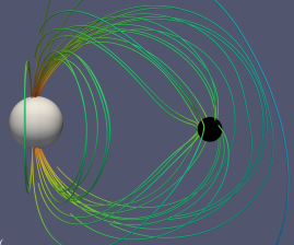
Figure 1: Interaction of a black hole (right) with the magnetic field lines of a neutron star (left) shortly before merger.

2 Methods

In this work, we model the magnetospheric dynamics of a BH–NS system. To do so, we need to take two aspects of the system into account: The plasma inside the magnetosphere, and the relativistic effects of the system, in particular, the BH and its ergosphere.
Sourced by the magnetic field of the NS, the orbital motion will trigger pair creation prior to merger (Hansen & Lyutikov, 2001; Lyutikov, 2019) making the magnetosphere nearly force-free (Goldreich & Julian, 1969). We can model its dynamics by adopting the force-free electrodynamics approximation (Palenzuela et al., 2010; Parfrey et al., 2013; Carrasco et al., 2019). Such an approximation is well justified in a closely orbiting system with sufficiently large magnetic fields (Hansen & Lyutikov, 2001; Lyutikov, 2019; Wada et al., 2020), and has been used extensively to study the pre-merger magnetosphere of compact binaries (Palenzuela, 2013; Dionysopoulou et al., 2013; Paschalidis et al., 2013; Palenzuela et al., 2013b, a; Ponce et al., 2015; East et al., 2021; Carrasco et al., 2021). We specifically make use of the formulation of Palenzuela et al. (2013b) as used in our previous studies (Most & Philippov, 2020, 2022a, 2022b).

The force-free electrodynamics conditions (Gruzinov, 1999) are enforced using an effective parallel conductivity term (Alic et al., 2012; Spitkovsky, 2006). We then solve the discrete form of the general-relativistic force-free electrodynamics system using a high-order finite-volume scheme (McCorquodale & Colella, 2011) with WENO-Z reconstruction (Borges et al., 2008). The numerical code is implemented on top of the adaptive mesh-refinement infrastructure of the AMReX framework (Zhang et al., 2019). More details on this implementation can be found in Most & Philippov (2022a).

Secondly, we need to model the orbiting binary system, including the near-horizon geometry of the BH. Several approaches have been proposed in the literature. It is possible to model the BH as a resistive surface using the approximate membrane-paradigm (Thorne et al., 1986). Such approaches have been used in flat spacetime to model BH flares from interactions with coronal magnetic fields (e.g., Yuan et al., 2019). At the same time, these can only approximately capture the ergospheric dynamics operative in the BH magnetosphere (Komissarov, 2004). Alternatively, it has been successfully demonstrated that the common magnetosphere of the system can be modeled as a Kerr spacetime (Kerr, 1963) with the NS (modeled as a spherical conductor) moving on a point-particle orbit (Carrasco et al., 2021). While this captures the necessary BH dynamics, it only approximately models the orbit and the NS. Finally, it would also be possible to resort to fully dynamical spacetime simulations of the system (East et al., 2021). While these can capture all the necessary aspects mentioned above, solving the Einstein equations is computationally expensive. It typically prevents the use of very high numerical resolution necessary to avoid spurious diffusion in the magnetosphere.
In this study, we use a third way, in between a stationary spacetime approach and a full numerical relativity simulation. Following Paschalidis et al. (2013), we make use of numerical relativity initial conditions for such a system, constructed by imposing a helical Killing vector, i.e., constant orbital separation (Grandclement, 2006; Taniguchi et al., 2007, 2008; Foucart et al., 2008).

	$\Omega$ [$\rm s^{-1}$]	$a\,\left[\rm km\right]$	$\chi_{\rm BH}$	$\theta_{\rm NS}[^{\circ}]$
NSBH_$\chi$085_60_60	925.3.0	103.3	0.85	60
NSBH_$\chi$085_60_70	765.0	103.3	0.85	60
NSBH_$\chi$085_60_80	637.0	118.1	0.85	60
NSBH_$\chi$-06_60	928.2	89.9	-0.60	60
NSBH_$\chi$-03_60	928.2	89.9	-0.30	60
NSBH_$\chi$0_60	928.2	89.9	0.00	60
NSBH_$\chi$03_60	928.2	89.9	0.30	60
NSBH_$\chi$85_60	928.2	89.9	0.85	60
GW200115${}^{\ast}\_0$	996.7	89.9	-0.30	0
GW200115${}^{\ast}\_30$	996.7	89.9	-0.30	30
GW200115${}^{\ast}\_45$	996.7	89.9	-0.30	45
GW200115${}^{\ast}\_60$	996.7	89.9	-0.30	60
GW200115${}^{\ast}\_90$	996.7	89.9	-0.30	90

Table 1: Summary of the black hole (BH) – neutron star (NS) binaries considered in this work. The columns denote the orbital angular frequency $\Omega$, the orbital separation $a$, the dimensionless BH spin $\chi_{\rm BH}$ perpendicular to the orbital plane, and the NS dipole inclination relative to the orbital angular momentum axis. We further adopt canonical masses of $m_{\rm BH}=5\,M_{\odot}$ and $m_{\rm NS}=1.4\,M_{\odot}$ for the BH and NS, respectively. The NS is assumed to be irrotational. Because of the decoupling of electromagnetic and gravitational sectors in our setup, the simulation results are scale-invariant under the magnetic field strength. For our fiducial GW200115-like models we adopt negative spins consistent with the original detection paper Abbott et al. (2021), but caution that their astrophysical interpretation remains uncertain (Mandel & Smith, 2021).

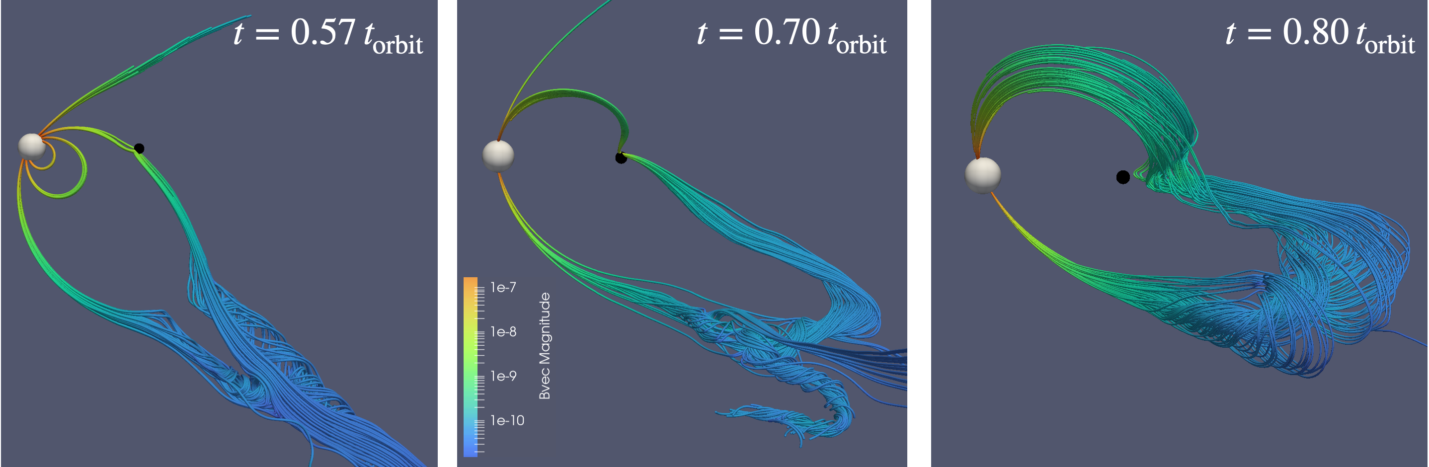
Figure 2: Three-dimensional magnetic field line visualization of a flaring event for a GW200115-like binary with a magnetic dipole with $\theta_{\rm NS}=60^{\circ}$ inclination. Shown are selected field line bundles for three different times, $t$, relative to the orbital period, $t_{\rm orbit}$. (Left) Closed magnetic field lines get initially accreted and pinned onto the black hole. (Center) Continued orbital motion begins twisting the connected field lines, inflating the connected flux tube. (Right) The flare detaches from the binary as can be seen by field lines disconnecting from the black hole (due to reconnection in trailing current sheet). The strong twist is visible as a toroidal component of the inflated flux tube. Colors indicate logarithmic magnetic field strengths in relative units.

More concretely, we solve the extended-conformal-traceless-sandwich formulation for a BH–NS system (Taniguchi et al., 2008; Tacik et al., 2016) with Cook-Pfeiffer boundary conditions on the black hole (Cook & Pfeiffer, 2004; Caudill et al., 2006). We highlight that this choice of initial data allows us to perform simulations at fixed orbital separation in full general relativity, representing the most natural extension of our flat spacetime setup to full general-relativity (Most & Philippov, 2022a). Numerically, this system is solved using the FUKA code (Papenfort et al., 2021), which operates on top of the spectral Kadath framework (Grandclement, 2010). The resulting initial data is directly interpolated onto our computational grid using the spectral representation. The interior of the black hole is filled using eighth-order Lagrange extrapolation (Etienne et al., 2007).
To evolve these initial conditions using force-free electrodynamics we need to perform two modifications. First, we need to identify the surface of the NS in order to impose boundary conditions for the force-free electrodynamics evolution of the magnetosphere. This is done approximately by identifying a level surface of the rest-mass density, $\rho\simeq 10^{-6}\rho_{\rm max}$, where $\rho_{\rm max}$ is the maximum rest-mass density inside the neutron star.
Second, following our previous approach in flat spacetimes (Most & Philippov, 2022a), we solve the extended Maxwell system also inside the neutron star by imposing ideal magnetohydrodynamics conditions on the electric field, ${\bf E}=-{\bf v}\times{\bf B}$. This requires a prescription for the three-velocity, ${\bf v}$, of the spacetime foliation. In principle, the velocity field can be self-consistently obtained from the numerical initial conditions. However, it is currently not known how to self-consistently impose a velocity field corresponding to perfect uniform rotation (Tichy, 2011, 2012). Indeed, we have found that when evolving these consistent velocity profiles small non-uniformities in the electric field close to the surface lead to a spurious diffusion of the magnetic field out of the NS. This motivated us to manually replace the velocity profile with that of perfect uniform rotation consistent with the rotation frequency of star prescribed in the initial conditions. Since we are keeping both spacetime and hydrodynamics fixed, this amounts to merely modifying the boundary conditions at the surface of the star. Indeed, we could equivalently have opted to excise the stellar interior and impose those boundary conditions only on the surface instead (Carrasco et al., 2019).

3 Results

In the following, we will present our results on the evolution of the joint BH-NS magnetosphere and electromagnetic precursor flares emitted from them. These are based on performing systematic numerical studies of general-relativistic BH-NS magnetosphere dynamics for the models listed in Tab. 1. While we will mainly focus on a fiducial system consistent with the GW200115 event (Abbott et al., 2021), we will also present a parameter study in terms of BH spin and binary separation, allowing us to generalize our findings to arbitrary systems with realistic mass ratios.
The present work is divided into several parts. First, we begin by describing the flares and flaring mechanism operating inside the BH–NS magnetosphere (Sec. 3.1). We then discuss its dependence on the magnetic field topology (Sec. 3.2), and finish with a discussion on potentially observable signatures of these flares (Sec. 3.3).

3.1 Precursor flares from the late of inspiral of black hole – neutron star binaries

In this Section, we will describe the generic flaring mechanism operating in the magnetosphere of a GW200115-like system.
We start out with a description of the common pre-merger magnetosphere. In this regime, the magnetic field lines of the NS can thread the BH, establishing a connected flux tube between the two compact objects in the binary system (see Fig. 1). This process will happen regardless of the orientation of the NS magnetic field. This is in contrast to NS-NS pre-merger magnetospheres (Most & Philippov, 2020, 2022a), where a minimal degree of misalignment between the two stellar magnetic moments is required in order to establish connected flux tubes (Cherkis & Lyutikov, 2021). Orbital motion of the system can then lead to a build-up of twist in these connected loops, causing them to inflate (Most & Philippov, 2020). However, unlike for the NS, which is a perfect conductor, the BH allows for field line slippage (MacDonald & Thorne, 1982; Thorne et al., 1986). Furthermore, since a BH cannot support closed field lines anchored solely in it (MacDonald & Thorne, 1982), the effective field geometry on the BH will have both open (split-monopole-like) and closed (flux tubes connected to the NS) field lines. Within this magnetosphere, a current sheet will form, causing electromagnetic energy to be dissipated. The extent of this current sheet is larger than that of a rotating BH (Komissarov & McKinney, 2007). We attribute this to the presence of the orbital motion making the local magnetosphere of the BH more closely resemble that of a boosted BH configuration (Carrasco et al., 2019). The energetics of the dissipation in the individual magnetospheres have been extensively studied by Carrasco et al. (2021), and we will not focus on those aspects associated with the energy dissipation of each individual compact object here. Rather, we will describe the dynamics of the common flux tube, which – as we will demonstrate – is able to give rise to realistic scenarios for EM transients, akin to NS-NS magnetospheres (Most & Philippov, 2022b).
The general dynamics of the connected flux tube in the BH-NS pre-merger magnetosphere is shown in Fig. 2. There, we focus on the dynamics of a GW200115-like binary with a NS magnetic moment inclined by $\theta_{\rm NS}=60\,^{\circ}$ relative to the orbital angular momentum axis (see Tab. 1 for details). While flaring will happen periodically, with about two flares being emitted per orbit (Cherkis & Lyutikov, 2021), we will first focus on a single flaring event.
Starting with the situation shown in the left panel of Fig. 2, we can see that due to orbital motion the closed zone of the NS magnetosphere will start to interact the BH. As we show in Sec. 3.2, it will be crucial that the BH interacts with field lines forming the outer part of the magnetosphere, i.e., field lines being close to the orbital light cylinder. As the binary continues to orbit, an effective twist is built-up and the connected flux tubes begin to inflate (Fig. 2, middle panel). We can see that the dynamics of connected field lines closer to the orbital light cylinder differ from those further inwards . This is mainly a result of the different field strengths of the flux tubes connecting the NS and BH. While the shorter flux tube slowly inflates, the larger flux tube extends further outwards. As indicated by the color coding, the smaller flux tube (green color) has higher field strengths compared to the lower one (blue color). This means that the same twist applied to each flux tube will lead to a different morphology. As can be seen in the final panel of Fig. 2, the longer flux tube gets strongly twisted and contains a strong toroidal field component, visually showing the twist. It is this outer part at lower field strengths (blue color), which will detach and flare. The upper loop does not show any deformation. Instead, because of dissipation in the trailing current sheet (Lyutikov & McKinney, 2011), we observe a steady state twist in this case. Since force-free models do not support plasma pressure, current sheets may collapse quicker and dissipate more, compared to current sheets in a fully kinetic description.
This lets us draw an important conclusion. While BH-NS systems can naturally flare, the flaring will likely release energy build-up around the orbital light cylinder (i.e., in the lower field strengths part of the magnetosphere). This is different from NS-NS systems, in which flux tubes deep insight the orbital light cylinder will flare (Most & Philippov, 2022a). The amount of energy released in a flare (or even whether flaring happens at all), will then depend on the relative inclination of the magnetic moment of the star relative to the orbital rotation axis. We will quantify this in Sec. 3.2.

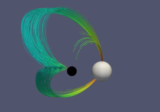
Figure 3: Three-dimensional magnetic field line visualization of a flaring event for a GW200115-like binary for a magnetic dipole with $\theta_{\rm NS}=30^{\circ}$ inclination at a time $t\simeq t_{\rm orbit}$, where $t_{\rm orbit}$ is the orbital period. Shown are selected field line bundles that highlight the presence of the equatorial current sheet. Unlike larger magnetic dipole inclinations, efficient reconnection in this current sheetself-limits the twist imposed on the flux tubes. The configuration shown here is in a quasi-steady state, and no flaring is observed.

3.2 Importance of magnetic field inclination

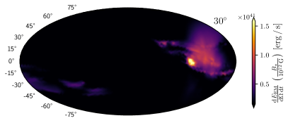
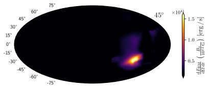
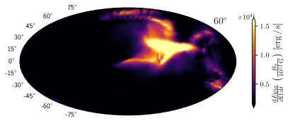
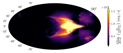
Figure 4: Spherical projection of the average outgoing electromagnetic energy flux density of the flares for various inclinations, $\theta_{\rm NS}$, of the neutron star’s dipole magnetic field extracted at a radius $r=500\,\rm km$. The background flux has been subtracted. From top left to bottom right, we show cases for $\theta_{\rm NS}=30^{\circ}$ (top left), $45^{\circ}$ (top right), $60^{\circ}$ (bottom left) and $90^{\circ}$ (bottom right).

Having described the flaring mechanism operating in a BH-NS magnetosphere prior to the merger, we now proceed with describing the characteristic properties of the flares. In doing so, we will highlight the importance of the inclination of the NS magnetic moment for the flaring mechanism.
Since there are no direct a priori constraints on the orientation of premerger magnetic fields, we consider a range of magnetic field inclinations $\theta_{\rm NS}=[0^{\circ},30^{\circ},45^{\circ},60^{\circ},90^{\circ}]$. Statistically, this angle of inclination is expected to correlate with the age of the pulsar (Tauris & Manchester, 1998; Young et al., 2010). All models are listed in Table 1. Depending on this inclination angle, we find two general outcomes: For inclinations above $45^{\circ}$ our simulations reveal a flaring state as described before and shown in Fig. 2. For inclinations $\theta_{\rm NS}\lesssim 45^{\circ}$, we, on the other hand, find no flaring. Instead, a constant state of dissipation in the current sheet around the BH sets in, leading to the build-up of a steady twist, as shown in Fig. 3. We point out that this is likely enhanced by the fact that the current sheet is enlarged due to orbital motion, compared to an isolated spinning BH. Compared with Fig. 2, where flaring occurred at low field strength field lines (blue color), the $\theta_{\rm NS}=30^{\circ}$ system (see Fig. 3) twists only inner field lines at higher field strengths (green colors). Similar to the shorter twisted flux tubes in Fig. 2, the orbital motion is insufficient to cause these field lines to inflate and twist. Indeed, this system (and any system at lower inclination) does not flare. This situation is loosely similar to the polar flaring dynamics of magnetar explosions (Parfrey et al., 2013; Carrasco et al., 2019). For these, Mahlmann et al. (2023) have recently shown that depending on the latitude of the footpoint of the twisted flux tube, it will either flare or become kink-unstable, thereby dissipating part of the twist. The distinction between the two states directly results from the different locations inside the magnetosphere that experience the twist. Polar field lines experience less pressure from confining magnetospheric field lines, and will more easily flare, i.e., produce an electromagnetic outflow. In the case of the BH-NS systems considered here, the role of latitude is played by the inclination angle of the NS’s magnetic moment. In summary, we find that a minimum inclination angle $\theta_{\rm NS}\simeq 45^{\circ}$ may be necessary for flaring, although the precise behavior will also depend on the dissipation rate inside the current sheet. In this sense our results should be interpreted as a lower limit on the amount of flaring.
The results of a parameter survey for these systems are shown in Fig. 4, which show the time-integrated energy fluxes per spherical angle on a sphere at radius $r\,\simeq 500\,\rm km$ from the orbital axis. Rather than showing the flux for a given time, we have averaged the Poynting flux density over one flaring event. Beginning with the $\theta_{\rm NS}=30^{\circ}$ case (top left) we can see that no clear flaring structure is present. There seems to be a tiny amount of residual emission associated with steady-state dissipation, potentially accompanied by the ejection of large plasmoids (Carrasco et al., 2021). Beginning with $\theta_{\rm NS}=45^{\circ}$, we instead see a clear flare structure emerging, i.e. a localized energy flux at high lattitude. The precise lattitude of the flare correlates directly with $\theta_{\rm NS}$, with flares being progressively emitted closer to the equator with increasing inclination, $\theta_{\rm NS}$. At the same time, we can also clearly observe an increase in strength and size of the flares for more strongly misaligned systems.
We can furthermore quantify the overall luminosity of the flares by integrating the previously shown Poynting flux densities over the spheres. In Fig. 5, we can indeed see that the system flares twice per orbit. Moreover, we confirm that the luminosity of more strongly inclined flares can be enhanced by a factor two, and that no detectable flaring is present in our simulation at small inclinations.

To better understand the expected behavior we need to establish a baseline for the luminosity emitted in these systems. We therefore compare the luminosity of the flares to the one emitted by the orbital motion of a vacuum dipole. This has been found to be (Hansen & Lyutikov, 2001; Ioka & Taniguchi, 2000),

$$\mathcal{L}_{\rm Dipole} =\frac{4}{15c^{5}}\mu^{2}a^{2}\Omega^{6}\,,$$ (1)

$$\approx 2.9\cdot 10^{39}\frac{{\rm erg}}{\rm s}\left(\frac{B_{\ast}}{10^{12}\,\rm G}\right)^{2}\left(\frac{M}{6.4\,M_{\odot}}\right)^{3}\left(\frac{90\,\rm km}{a}\right)^{7}\,,$$

where $B_{\ast}$ is the magnetic field strength at the neutron star surface, $M$ is the total mass of the system, and $a$ the binary separation. In simplifying the expression we have further assumed that (neglecting gravitational radiation reaction) the binary is on a Keplerian orbit (Peters, 1964), and that the magnetic moment $\mu=B_{\ast}R_{\ast}^{3}$, where $R_{\ast}=13\,\rm km$ (e.g., Özel & Freire (2016)). Based on this estimate, the flares present in our simulations are up to a $100$-times more luminous than the expected orbital emission. On the contrary, our non-flaring simulations are indeed roughly consistent with the estimate (1), in line with results reported by Carrasco et al. (2021), who found an additional enhancement due to relativistic orbital motion of the NS. Overall, the luminosities expected for a surface magnetic field $B_{\ast}\simeq 10^{12}\,\rm G$ magnetic field will be roughly comparable to luminosities $\mathcal{L}_{\rm EM}=10^{41}\,\rm erg/s$.

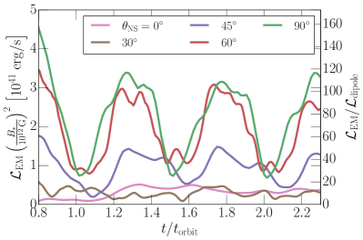
Figure 5: Electromagnetic luminosities, $\mathcal{L}_{\rm EM}$, for GW200115-like models for various inclination angles, $\theta_{\rm NS}$, of the neutron star’s magnetic field. Normalizations are given relative to the moving dipole estimate, $\mathcal{L}_{\rm dipole}$, see also (1), as well as to the orbital period, $t_{\rm orbit}$. All luminosities have been computed at a distance $r=500\,\rm km$ from the system.

Having quantified the energetics of individual flares and their dependency on the inclination angle $\theta_{\rm NS}$, we conclude this discussion by clarifying the role of the other system parameters, notably (dimensionless) BH spin, $\chi_{\rm BH}$, and orbital separation $a$.
We first consider the impact of BH spin, $\chi_{\rm BH}$, as shown in the upper panel of Fig. 6. We find that the flare luminosities do not seem to depend on the BH spin. This is consistent with the flaring dynamics being governed by the orbital motion, not the extent of the ergosphere, which does depend on spin. It also matches earlier work on constant emission from BH-NS systems (Carrasco et al., 2021). In more aligned cases, it might be possible that ergospheric motions for high spin BHs could be able to continuously twist connected flux tubes, akin to what is expected in models of magnetic loops connecting BHs and thin accretion flows (Galeev et al., 1979; Uzdensky & Goodman, 2008; Yuan et al., 2019). However, even when simulating models with BH spins of $\chi_{\rm BH}=0.85$ with partially aligned or fully aligned magnetic moment we do not find signs of flaring. On the other hand, our resistive force-free electrodynamics might be too diffusive compared to a fully kinetic description of collisionless relativistic pair plasma (Parfrey et al., 2019).

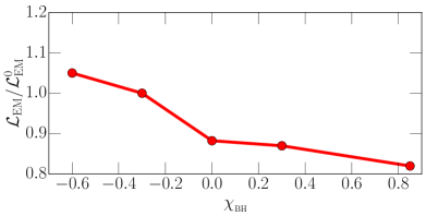
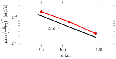
Figure 6: Bulk electromagnetic luminosity of the flares, $\mathcal{L}_{\rm EM}$. (Top) Scaling with black hole spin, $\chi_{\rm BH}$, relative to the luminosity, $\mathcal{L}_{\rm EM}^{0}$, of the aligned system.(Bottom) Dependence on orbital separation, $a$, with absolute magnitudes scaled to a surface field strength $B_{\ast}=10^{12}\,\rm G$.

We next focus on the dependency on the orbital separation, $a$. According to the estimate presented for the moving dipole, Eq. (1), we expect the luminosity to scale as $\mathcal{L}_{\rm EM}\propto a^{-7}$. Comparing this with our simulations, we indeed find good agreement with this scaling, in line with previous studies of continuous emission (Carrasco et al., 2021). This strengthens the observation made above that the flaring is mainly associated with the motion of the NS, rather than a relative twist interaction as seen in the NS-NS case (Most & Philippov, 2020). We caution that this scaling may be modified as the binary approaches merger, i.e., on the last orbit. Full numerical relativity simulations of the merger will be needed to clarify this point (East et al., 2021).

Finally, we can also comment on the impact of mass ratio. While lighter BHs are astrophysically less likely due to the presumed existence of a lower mass gap (e.g., Farr et al. 2011; Ozel et al. 2012, but see also Abbott et al. (2020) for a counterexample), it may be interesting to ask what the impact of more massive BHs in NS-BH system would be for the dynamics outlined here. To do so, we point out that the magnetospheric activity and its associated luminosity, $\mathcal{L}_{\rm EM}$, is governed by the orbital separation $a$, since $a$ determines the location relative to the NS’s dipole field and therefore the strength of the field lines the BH is interacting with. To lowest order, the orbital separation will change over time, $t$, according to (Peters, 1964),

$$a\left(t\right)=a_{0}\left(1-\frac{t}{t_{\rm merger}}\right)^{1/4}\,,$$ (2)

where $a_{0}$ is the initial separation with corresponding time to merger,

$$t_{\rm merger}=\frac{5}{256}\frac{a_{0}^{4}}{m_{\rm NS}^{3}Q\left(1+Q\right)}\,,$$ (3)

with, $Q=m_{\rm BH}/m_{\rm NS}>1$, being the mass ratio. This means that the time to merger, $t_{\rm merger}\sim\left(Q^{2}+Q\right)^{-1}$, is shorter for more massive systems. Since the inspiral will accelerate towards the merger, the system will therefore spent fewer time in very close orbit (relative to the radial decay of the NS’s magnetic field), and will – in principle – have EM outflows at lower luminosities. We quantify this explicitly in the next section. Since our simulations have BHs with masses close to the lower mass gap, our results can naturally be seen as upper bounds in terms of mass ratio dependence.

3.3 Observational implications

In the following, we want to provide a few simple estimates aimed at assessing the potential observable impact of flares emitted from the inspiralling NS-BH system. We begin by estimating the number of potentially observable flares, $N_{\rm flares}$, following our discussion in Most & Philippov (2022a). Since the binary is emitting two flares per orbit, the number of flares starting from a given separation, or equivalently from a given orbital frequency, will be the same as the number of gravitational wave cycles. Using Kepler’s law and the separation scaling consistent with the simulations (see Fig. 6), we can estimate the frequency, $f_{\rm min}$, for which the luminosity reaches a threshold value, $\mathcal{L}_{\rm min}$, necessary for obtaining an observable signal. Overall, we find

$$f_{\rm min}=\frac{1}{2\pi}\frac{\sqrt{M}}{a_{0}^{3/2}}\left(\frac{\mathcal{L}_{\rm min}}{\mathcal{L}_{0}}\right)^{3/14}\,.$$ (4)

For an inspiralling compact binary, we can to lowest order estimate the number of gravitational wave cycles, $N_{\rm GW}$ (Maggiore, 2008),

$$N_{\rm flares} =N_{\rm GW}\simeq\frac{1}{32\pi^{8/3}}\left(\mathcal{M}f_{\rm min}\right)^{-5/3}\,,$$ (5)

$$\simeq 2\ \left(\frac{B}{10^{12}\,\rm G}\right)^{5/7}\left(\frac{10^{42}\ \rm erg/s}{\mathcal{L}_{\rm min}}\right)^{5/14}\left(\frac{\sigma}{10^{-3}}\right)^{5/14}\,,$$ (6)

where the latter is obtained for a GW200115-like system. We have further introduced a parameter, $\sigma=10^{-3}$, estimating the efficiency of converting the outgoing luminosity into observable radiation (see Most & Philippov (2022a) for a discussion). We point out that this estimate is about ten-times lower than in the binary neutron star case (Most & Philippov, 2022a), but can reach the same order, if NS field strengths $B_{\ast}\simeq 10^{13}\,\rm G$ are present. This finding is overall consistent with the fact, that the last orbits prior to merger will happen at almost twice the orbital separation compared to the NS-NS case. The flaring process of outer field lines then in turn will only involve outer, lower field strengths regions of the closed NS magnetosphere. In addition, NS-NS merger flaring features a shallower separation dependence, $\mathcal{L}^{\rm NS-NS}_{\rm EM}\sim a^{-3/5}$ (Most & Philippov, 2020). We can also explicitly quantify the dependence on the mass ratio, $Q$, which we find to be $N_{\rm flares}\sim Q^{-1}\left(1+Q\right)^{-1/2}$. This implies that flares may not leave observable signatures for larger mass ratios with $N_{\rm flares}\lesssim 1$ for $Q\gtrsim 6$.

How do flares convert their energy into transients?
Having clarified the number of flares expected from the late inspiral of a realistic BH-NS binary, we now discuss the potential emission channels open to converting the energy of the flares into observable transients.

First, we focus on the production through forced reconnection in the orbital current sheet. Reconnection is enhanced due to forcing in the outer parts of the field lines, leading to the copious ejection of plasmoids. The merger of these plasmoids can convert a sizeable fraction of the available energy into low frequency electromagntic waves (Philippov et al., 2019). Dissipation of magnetic energy due to reconnection in the current sheet leads to X-ray emission (Beloborodov, 2021). Although resistive dissipation can only be approximately captured in our simulations, we conservatively measure an upper bound of $\mathcal{L}_{\rm diss}\lesssim 0.3\mathcal{L}_{\rm EM}$, consistent with our previous work on NS-NS systems (Most & Philippov, 2020, 2022a).
Focusing on the flares, two main scenarios of the low frequency coherent emission are possible. Either the flares propagate out to large distances, where they will interact with the binaries pair wind. Such a scenario has been shown to be capable of producing Fast Radio Bursts in the case of magnetars (Beloborodov, 2017; Metzger et al., 2019), albeit we here are faced with the prospect of having far less energetical flares.
In the second scenario, the flares can depending on the inclination angle, $\theta_{\rm NS}$, of the NS’s magnetic moment be emitted along the equatorial plane (see Fig. 4), where they will eventually collide with the orbital current sheet. The compression of the sheet results in the formation of plasmoids and the launching of small-scale fast waves with wavelength potentially in the radio band (Lyubarsky, 2020). Such a scenario has been proposed for FRB emission in magnetars and has recently been investigated numerically using kinetic simulations (Mahlmann et al., 2022). We caution that interacting compact binaries may produce FRB-like transients also by other means (for a comprehensive recent review see, e.g., Zhang (2022)). Since some of these will depend on kinetic or magnetohydrodynamic (MHD) physics (i.e., finite magnetization and shock formation) not included in our force-free simulations, we do not consider them here. In an earlier work, we have numerically investigated the flare collision dynamics for NS-NS systems, showing the feasibility of this mechanism to produce Fast Radio Burst-like transients (Most & Philippov, 2022b).
In the following, we will apply this model to the BH-NS parameters extracted from our simulations as well. We begin by computing the effective Lorentz factor, $\Gamma$, of the plasma in the flare. Following Lyubarsky (2020), we can estimate $\Gamma=\sqrt{B_{\rm flare}/B_{\rm wind}}\approx 1.6$, where we have used that in our simulation the flaring field strength $B_{\rm flare}=5\times 10^{8}\,B_{12}^{\ast}\,\rm G$ ist ten-times larger than the wind strength $B_{\rm wind}$, where $B_{12}^{\ast}=B_{\ast}/10^{12}\,\rm G$ is the surface magnetic field strength. As the flare collides with the current sheet, it triggers enhanced plasmoid formation and production of low frequency fast magnetosonic waves. In highly magnetized plasma these waves can propagate even at frequencies below the plasma frequency. Morever, since they propagate on top of the wind, they avoid damping expected for GHz waves in the inner magnetosphere (Beloborodov, 2023). The frequency of the resulting emission due to plasmoid collision is then inversely proportional to the plasmoid size (Lyubarsky, 2020). Since our simulations do not correctly capture collisionless reconnection physics, we translate results of small-scale kinetic simulations (Mahlmann et al., 2022) to compact binary magnetospheres (Most & Philippov, 2022b). For this scenario, it can then be shown that the characteristic emission frequency (Lyubarsky, 2020),

$$\nu_{\rm FRB}=\frac{1}{2\pi\xi\zeta}\sqrt{\frac{2r_{e}}{3\beta_{\rm rec}c\Gamma}\omega_{B}^{3}}\simeq 9\,\left(B^{\ast}_{12}\right)^{3/2}\,\rm GHz\,.$$ (7)

Here we have introduced the electron gyrofrequency in the flare via $\omega_{B}=eB_{\rm flare}/m_{e}c$, where $e$, $m_{e}$ and $r_{e}$ are the electron charge, mass and classical radius, respectively. We have also used $\xi\zeta\approx 100$ (Mahlmann et al., 2022), as well as a reconnection rate $\beta_{\rm rec}\simeq 0.1$ (Sironi & Spitkovsky, 2014; Guo et al., 2015). These estimates imply that for surface field strength $B_{\ast}\simeq 10^{12}\,\rm G$, Fast-Radio-Burst-like transients can indeed be launched, albeit only for about two flaring events, likely happening in the last orbit, see Eq. (6). Conversely, if the field strength was increased to achieve multiple flaring episodes, these would quickly go outside of the radio band. We caution that the exact frequency value will strongly depend on the radial distance at which the flare hits the orbital current sheet (see Most & Philippov (2022b) for a discussion).

4 Conclusions

Apart from gravitational wave emission, compact binary inspirals could be accompanied by electromagnetic precursors sourced prior to merger (Hansen & Lyutikov, 2001; Lai, 2012; Piro, 2012; Lyutikov, 2019). These could be produced as a result of dynamical interactions in the common magnetosphere (Lai, 2012; Piro, 2012; Palenzuela et al., 2013b, a; Ponce et al., 2015; Most & Philippov, 2020, 2022a), tidal deformation of the NSs crust (Tsang et al., 2012), or as a result of partially expelling the magnetosphere after the merger (balding transient) (Nathanail, 2020; East et al., 2021). All these scenarios have in common that they will feature some dependence on the magnetic field topology, and the spin present in the initial system. Since they are either not well constrainable from the gravitational wave signal , or in the case of the magnetic field topology might get destroyed during merger (Aguilera-Miret et al., 2020), such precursors might offer one of the few glimpses into the system. Even more so, sky localization of gravitational wave events currently suffers from large uncertainties impeding swift follow-up observations. If radio transients were sourced by the merger, this would potentially enable fast localization by means of all-sky radio observations (Sachdev et al., 2020; Wang et al., 2020; Yu et al., 2021).
In this work, we have investigated such a scenario for BH-NS binaries, in particular realistic configurations for which likely no remnant baryon mass, which could power additional transient, will be present. By means of general-relativistic force-free electrodynamic simulations we have demonstrated that relative orbital motions will naturally form closed magnetic flux tubes, the twisting of which causes them to erupt akin to solar coronal mass ejections (Chen, 2011). We find that the emission of flares correlates with the part of the closed magnetosphere closest to the orbital light cylinder. These field lines may be sheared more easily, leading to an easier flaring. More specifically, we find that magnetic field inclinations of $45^{\circ}$ and larger will lead to strong outbursts. For aligned systems, we instead find that the black hole continuously dissipated energy establishing a steady state twist. This effect seems to get enhanced by the orbital motion, rather than by BH spin, which instead controls the size of the ergosphere. We caution that the precise picture might change when collisionless reconnection physics is properly accounted for, either by means of kinetic (Philippov et al., 2015; Kalapotharakos et al., 2018), two-fluid simulations (Wang et al., 2018; Dong et al., 2019) or even in ideal MHD, necessitating novel formulations in the relativistic context (Most et al., 2022).
On the quantitative side, we find that flares manage to significantly enhance the electromagnetic luminosity compared to the orbiting dipole estimate (Ioka & Taniguchi, 2000; Hansen & Lyutikov, 2001). This is in line with previous work on BH-NS (Carrasco et al., 2021) and NS-NS magnetospheres Most & Philippov (2020, 2022a). Concretely, we find that magnetic field strengths of $B_{\ast}=10^{12}\,\rm G$ at the stellar surface, correspond to luminosities around $\mathcal{L}_{\rm EM}\simeq 10^{41}\,\rm erg/s$. This scales strongly with the separation (but not BH spin), consistent with previous analytical and numerical calculations for continuous electromagnetic emission from BH-NS mergers (Carrasco et al., 2021). Overall, we estimate that this leads to at most two potentially detectable flares when using the parameters listed above. However, their emission, if driven by current sheet – flare interactions (Lyubarsky, 2020; Mahlmann & Aloy, 2021; Most & Philippov, 2022b), will likely correspond to that of fast radio burst-like transients, peaking in the $\nu=9\,\rm GHz$ range, making them interesting targets for all-sky radio observatories (Callister et al., 2019; James et al., 2019). More precise studies, which also account for systems with orbital precession will be needed to clarify the uncertainties in the present estimates, which largely depend on the radial location of the interaction of flares with the current sheet. While this work has largely considered flares as the main source of EM transients, larger Poynting flux outflows can also be produced at merger (D’Orazio & Levin, 2013; Mingarelli et al., 2015; D’Orazio et al., 2016; Nathanail, 2020; East et al., 2021). However, it remains uncertain how exactly these outflows would dissipate and, hence, what exact observable signatures they would correspond to. We plan to address such configurations in a future work.

The main challenge compared to NS-NS systems fundamentally lies in the expected mass ratio of these sytems (Fragione, 2021; Biscoveanu et al., 2022). Since the binary will orbit at larger separations compared to an equal mass system, the BH will fundamentally only interact with the outermost field lines of the NS, which flare more easily. Whether or not interactions with field lines closer to the star could lead to flaring remains unclear, due to the dissipative nature of the resistive force-free approach (Mahlmann et al., 2021). Future work will be needed to clarify these points.

References

- Abbott et al. (2017) Abbott, B. P., et al. 2017, Astrophys. J. Lett., 848, L13, doi: 10.3847/2041-8213/aa920c
- Abbott et al. (2020) Abbott, R., et al. 2020, Astrophys. J. Lett., 896, L44, doi: 10.3847/2041-8213/ab960f
- Abbott et al. (2021) —. 2021, Astrophys. J. Lett., 915, L5, doi: 10.3847/2041-8213/ac082e
- Aguilera-Miret et al. (2020) Aguilera-Miret, R., Viganò, D., Carrasco, F., Miñano, B., & Palenzuela, C. 2020, Phys. Rev. D, 102, 103006, doi: 10.1103/PhysRevD.102.103006
- Alexander et al. (2017) Alexander, K. D., et al. 2017, Astrophys. J. Lett., 848, L21, doi: 10.3847/2041-8213/aa905d
- Alic et al. (2012) Alic, D., Mosta, P., Rezzolla, L., Zanotti, O., & Jaramillo, J. L. 2012, Astrophys. J., 754, 36, doi: 10.1088/0004-637X/754/1/36
- Anand et al. (2021) Anand, S., et al. 2021, Nature Astron., 5, 46, doi: 10.1038/s41550-020-1183-3
- Beloborodov (2017) Beloborodov, A. M. 2017, Astrophys. J. Lett., 843, L26, doi: 10.3847/2041-8213/aa78f3
- Beloborodov (2021) —. 2021, Astrophys. J., 921, 92, doi: 10.3847/1538-4357/ac17e7
- Beloborodov (2022) —. 2022. https://arxiv.org/abs/2210.13509
- Beloborodov (2023) —. 2023. https://arxiv.org/abs/2307.12182
- Bildsten & Cutler (1992) Bildsten, L., & Cutler, C. 1992, Astrophys. J., 400, 175, doi: 10.1086/171983
- Biscoveanu et al. (2022) Biscoveanu, S., Landry, P., & Vitale, S. 2022, Mon. Not. Roy. Astron. Soc., 518, 5298, doi: 10.1093/mnras/stac3052
- Borges et al. (2008) Borges, R., Carmona, M., Costa, B., & Don, W. 2008, Journal of Computational Physics, 227, 3191, doi: 10.1016/j.jcp.2007.11.038
- Bransgrove et al. (2021) Bransgrove, A., Ripperda, B., & Philippov, A. 2021, Phys. Rev. Lett., 127, 055101, doi: 10.1103/PhysRevLett.127.055101
- Broderick et al. (2020) Broderick, J. W., et al. 2020, Mon. Not. Roy. Astron. Soc., 494, 5110, doi: 10.1093/mnras/staa950
- Callister et al. (2019) Callister, T. A., Anderson, M. M., Hallinan, G., et al. 2019, Astrophys. J. Lett., 877, L39, doi: 10.3847/2041-8213/ab2248
- Carrasco et al. (2021) Carrasco, F., Shibata, M., & Reula, O. 2021, Phys. Rev. D, 104, 063004, doi: 10.1103/PhysRevD.104.063004
- Carrasco et al. (2019) Carrasco, F., Viganò, D., Palenzuela, C., & Pons, J. A. 2019, Mon. Not. Roy. Astron. Soc., 484, L124, doi: 10.1093/mnrasl/slz016
- Caudill et al. (2006) Caudill, M., Cook, G. B., Grigsby, J. D., & Pfeiffer, H. P. 2006, Phys. Rev. D, 74, 064011, doi: 10.1103/PhysRevD.74.064011
- Chen (2011) Chen, P. 2011, Living Reviews in Solar Physics, 8, 1
- Chen (2011) Chen, P. F. 2011, Living Reviews in Solar Physics, 8, 1, doi: 10.12942/lrsp-2011-1
- Cherkis & Lyutikov (2021) Cherkis, S. A., & Lyutikov, M. 2021, Astrophys. J., 923, 13, doi: 10.3847/1538-4357/ac29b8
- Chornock et al. (2017) Chornock, R., et al. 2017, Astrophys. J. Lett., 848, L19, doi: 10.3847/2041-8213/aa905c
- Cook & Pfeiffer (2004) Cook, G. B., & Pfeiffer, H. P. 2004, Phys. Rev. D, 70, 104016, doi: 10.1103/PhysRevD.70.104016
- Cooper et al. (2022) Cooper, A. J., Gupta, O., Wadiasingh, Z., et al. 2022, doi: 10.1093/mnras/stac3580
- Coughlin et al. (2020a) Coughlin, M. W., Dietrich, T., Antier, S., et al. 2020a, Mon. Not. Roy. Astron. Soc., 492, 863, doi: 10.1093/mnras/stz3457
- Coughlin et al. (2020b) Coughlin, M. W., et al. 2020b, Mon. Not. Roy. Astron. Soc., 497, 1181, doi: 10.1093/mnras/staa1925
- Cowperthwaite et al. (2017) Cowperthwaite, P. S., et al. 2017, Astrophys. J. Lett., 848, L17, doi: 10.3847/2041-8213/aa8fc7
- Dai (2019) Dai, Z. G. 2019, Astrophys. J. Lett., 873, L13, doi: 10.3847/2041-8213/ab0b45
- Dionysopoulou et al. (2013) Dionysopoulou, K., Alic, D., Palenzuela, C., Rezzolla, L., & Giacomazzo, B. 2013, Phys. Rev. D, 88, 044020, doi: 10.1103/PhysRevD.88.044020
- Dong et al. (2019) Dong, C., Wang, L., Hakim, A., et al. 2019, Geophysical Research Letters, 46, 11584
- D’Orazio et al. (2022) D’Orazio, D. J., Haiman, Z., Levin, J., Samsing, J., & Vigna-Gomez, A. 2022, Astrophys. J., 927, 56, doi: 10.3847/1538-4357/ac4bdb
- D’Orazio & Levin (2013) D’Orazio, D. J., & Levin, J. 2013, Phys. Rev. D, 88, 064059, doi: 10.1103/PhysRevD.88.064059
- D’Orazio et al. (2016) D’Orazio, D. J., Levin, J., Murray, N. W., & Price, L. 2016, Phys. Rev. D, 94, 023001, doi: 10.1103/PhysRevD.94.023001
- Drout et al. (2017) Drout, M. R., et al. 2017, Science, 358, 1570, doi: 10.1126/science.aaq0049
- East et al. (2021) East, W. E., Lehner, L., Liebling, S. L., & Palenzuela, C. 2021, Astrophys. J. Lett., 912, L18, doi: 10.3847/2041-8213/abf566
- Etienne et al. (2007) Etienne, Z. B., Faber, J. A., Liu, Y. T., Shapiro, S. L., & Baumgarte, T. W. 2007, Phys. Rev. D, 76, 101503, doi: 10.1103/PhysRevD.76.101503
- Farr et al. (2011) Farr, W. M., Sravan, N., Cantrell, A., et al. 2011, Astrophys. J., 741, 103, doi: 10.1088/0004-637X/741/2/103
- Foucart (2012) Foucart, F. 2012, Phys. Rev. D, 86, 124007, doi: 10.1103/PhysRevD.86.124007
- Foucart et al. (2018) Foucart, F., Hinderer, T., & Nissanke, S. 2018, Phys. Rev. D, 98, 081501, doi: 10.1103/PhysRevD.98.081501
- Foucart et al. (2008) Foucart, F., Kidder, L. E., Pfeiffer, H. P., & Teukolsky, S. A. 2008, Phys. Rev. D, 77, 124051, doi: 10.1103/PhysRevD.77.124051
- Fragione (2021) Fragione, G. 2021, Astrophys. J. Lett., 923, L2, doi: 10.3847/2041-8213/ac3bcd
- Galeev et al. (1979) Galeev, A. A., Rosner, R., & Vaiana, G. S. 1979, Astrophys. J., 229, 318, doi: 10.1086/156957
- Ghirlanda et al. (2019) Ghirlanda, G., et al. 2019, Science, 363, 968, doi: 10.1126/science.aau8815
- Goldreich & Julian (1969) Goldreich, P., & Julian, W. H. 1969, Astrophys. J., 157, 869, doi: 10.1086/150119
- Gourdji et al. (2020) Gourdji, K., Rowlinson, A., Wijers, R. A. M. J., & Goldstein, A. 2020, Mon. Not. Roy. Astron. Soc., 497, 3131, doi: 10.1093/mnras/staa2128
- Grandclement (2006) Grandclement, P. 2006, Phys. Rev. D, 74, 124002, doi: 10.1103/PhysRevD.74.124002
- Grandclement (2010) —. 2010, J. Comput. Phys., 229, 3334, doi: 10.1016/j.jcp.2010.01.005
- Gruzinov (1999) Gruzinov, A. 1999. https://arxiv.org/abs/astro-ph/9902288
- Guo et al. (2015) Guo, F., Liu, Y.-H., Daughton, W., & Li, H. 2015, Astrophys. J., 806, 167, doi: 10.1088/0004-637X/806/2/167
- Hajela et al. (2019) Hajela, A., et al. 2019, Astrophys. J. Lett., 886, L17, doi: 10.3847/2041-8213/ab5226
- Hallinan et al. (2017) Hallinan, G., et al. 2017, Science, 358, 1579, doi: 10.1126/science.aap9855
- Hansen & Lyutikov (2001) Hansen, B. M. S., & Lyutikov, M. 2001, Mon. Not. Roy. Astron. Soc., 322, 695, doi: 10.1046/j.1365-8711.2001.04103.x
- Harris et al. (2020) Harris, C. R., Millman, K. J., van der Walt, S. J., et al. 2020, Nature, 585, 357, doi: 10.1038/s41586-020-2649-2
- Hunter (2007) Hunter, J. D. 2007, Computing in Science & Engineering, 9, 90, doi: 10.1109/MCSE.2007.55
- Ioka & Taniguchi (2000) Ioka, K., & Taniguchi, K. 2000, Astrophys. J., 537, 327, doi: 10.1086/309004
- James et al. (2019) James, C. W., Anderson, G. E., Wen, L., et al. 2019, Mon. Not. Roy. Astron. Soc., 489, L75, doi: 10.1093/mnrasl/slz129
- Kalapotharakos et al. (2018) Kalapotharakos, C., Brambilla, G., Timokhin, A., Harding, A. K., & Kazanas, D. 2018, Astrophys. J., 857, 44, doi: 10.3847/1538-4357/aab550
- Kerr (1963) Kerr, R. P. 1963, Phys. Rev. Lett., 11, 237, doi: 10.1103/PhysRevLett.11.237
- Komissarov (2004) Komissarov, S. S. 2004, Mon. Not. Roy. Astron. Soc., 350, 407, doi: 10.1111/j.1365-2966.2004.07446.x
- Komissarov (2005) —. 2005, Mon. Not. Roy. Astron. Soc., 359, 801, doi: 10.1111/j.1365-2966.2005.08974.x
- Komissarov & McKinney (2007) Komissarov, S. S., & McKinney, J. C. 2007, Mon. Not. Roy. Astron. Soc., 377, L49, doi: 10.1111/j.1745-3933.2007.00301.x
- Lai (2012) Lai, D. 2012, Astrophys. J. Lett., 757, L3, doi: 10.1088/2041-8205/757/1/L3
- Lehner et al. (2012) Lehner, L., Palenzuela, C., Liebling, S. L., Thompson, C., & Hanna, C. 2012, Phys. Rev. D, 86, 104035, doi: 10.1103/PhysRevD.86.104035
- Levin et al. (2018) Levin, J., D’Orazio, D. J., & Garcia-Saenz, S. 2018, Phys. Rev. D, 98, 123002, doi: 10.1103/PhysRevD.98.123002
- Lyubarsky (2020) Lyubarsky, Y. 2020, Astrophys. J., 897, 1, doi: 10.3847/1538-4357/ab97b5
- Lyutikov (2019) Lyutikov, M. 2019, Mon. Not. Roy. Astron. Soc., 483, 2766, doi: 10.1093/mnras/sty3303
- Lyutikov & McKinney (2011) Lyutikov, M., & McKinney, J. C. 2011, Phys. Rev. D, 84, 084019, doi: 10.1103/PhysRevD.84.084019
- MacDonald & Thorne (1982) MacDonald, D., & Thorne, K. S. 1982, Mon. Not. Roy. Astron. Soc., 198, 345
- Maggiore (2008) Maggiore, M. 2008, Gravitational Waves: Volume 1: Theory and Experiments, Gravitational Waves (OUP Oxford). https://books.google.com/books?id=AqVpQgAACAAJ
- Mahlmann & Aloy (2021) Mahlmann, J. F., & Aloy, M. A. 2021, Mon. Not. Roy. Astron. Soc., 509, 1504, doi: 10.1093/mnras/stab2830
- Mahlmann et al. (2021) Mahlmann, J. F., Aloy, M. A., Mewes, V., & Cerdá-Durán, P. 2021, Astron. Astrophys., 647, A58, doi: 10.1051/0004-6361/202038908
- Mahlmann et al. (2022) Mahlmann, J. F., Philippov, A. A., Levinson, A., Spitkovsky, A., & Hakobyan, H. 2022, Astrophys. J. Lett., 932, L20, doi: 10.3847/2041-8213/ac7156
- Mahlmann et al. (2023) Mahlmann, J. F., Philippov, A. A., Mewes, V., et al. 2023. https://arxiv.org/abs/2302.07273
- Mandel & Smith (2021) Mandel, I., & Smith, R. J. E. 2021, Astrophys. J. Lett., 922, L14, doi: 10.3847/2041-8213/ac35dd
- Margutti et al. (2017) Margutti, R., et al. 2017, Astrophys. J. Lett., 848, L20, doi: 10.3847/2041-8213/aa9057
- Margutti et al. (2018) —. 2018, Astrophys. J. Lett., 856, L18, doi: 10.3847/2041-8213/aab2ad
- McCorquodale & Colella (2011) McCorquodale, P., & Colella, P. 2011, Communications in Applied Mathematics and Computational Science, 6, 1
- McWilliams & Levin (2011) McWilliams, S. T., & Levin, J. 2011, Astrophys. J., 742, 90, doi: 10.1088/0004-637X/742/2/90
- Metzger et al. (2019) Metzger, B. D., Margalit, B., & Sironi, L. 2019, Mon. Not. Roy. Astron. Soc., 485, 4091, doi: 10.1093/mnras/stz700
- Mingarelli et al. (2015) Mingarelli, C. M. F., Levin, J., & Lazio, T. J. W. 2015, Astrophys. J. Lett., 814, L20, doi: 10.1088/2041-8205/814/2/L20
- Mooley et al. (2018a) Mooley, K. P., et al. 2018a, Nature, 554, 207, doi: 10.1038/nature25452
- Mooley et al. (2018b) Mooley, K. P., Deller, A. T., Gottlieb, O., et al. 2018b, Nature, 561, 355, doi: 10.1038/s41586-018-0486-3
- Most et al. (2018) Most, E. R., Nathanail, A., & Rezzolla, L. 2018, Astrophys. J., 864, 117, doi: 10.3847/1538-4357/aad6ef
- Most et al. (2022) Most, E. R., Noronha, J., & Philippov, A. A. 2022, Mon. Not. Roy. Astron. Soc., 514, 4989, doi: 10.1093/mnras/stac1435
- Most et al. (2021) Most, E. R., Papenfort, L. J., Tootle, S., & Rezzolla, L. 2021, Astrophys. J., 912, 80, doi: 10.3847/1538-4357/abf0a5
- Most & Philippov (2020) Most, E. R., & Philippov, A. A. 2020, Astrophys. J. Lett., 893, L6, doi: 10.3847/2041-8213/ab8196
- Most & Philippov (2022a) —. 2022a, Mon. Not. Roy. Astron. Soc., 515, 2710, doi: 10.1093/mnras/stac1909
- Most & Philippov (2022b) —. 2022b. https://arxiv.org/abs/2207.14435
- Nathanail (2020) Nathanail, A. 2020, doi: 10.3847/1538-4357/ab7923
- Nathanail et al. (2017) Nathanail, A., Most, E. R., & Rezzolla, L. 2017, Mon. Not. Roy. Astron. Soc., 469, L31, doi: 10.1093/mnrasl/slx035
- Nicholl et al. (2017) Nicholl, M., et al. 2017, Astrophys. J. Lett., 848, L18, doi: 10.3847/2041-8213/aa9029
- Özel & Freire (2016) Özel, F., & Freire, P. 2016, Ann. Rev. Astron. Astrophys., 54, 401, doi: 10.1146/annurev-astro-081915-023322
- Ozel et al. (2012) Ozel, F., Psaltis, D., Narayan, R., & Villarreal, A. S. 2012, Astrophys. J., 757, 55, doi: 10.1088/0004-637X/757/1/55
- Palenzuela (2013) Palenzuela, C. 2013, Mon. Not. Roy. Astron. Soc., 431, 1853, doi: 10.1093/mnras/stt311
- Palenzuela et al. (2010) Palenzuela, C., Lehner, L., & Liebling, S. L. 2010, Science, 329, 927, doi: 10.1126/science.1191766
- Palenzuela et al. (2013a) Palenzuela, C., Lehner, L., Liebling, S. L., et al. 2013a, Phys. Rev. D, 88, 043011, doi: 10.1103/PhysRevD.88.043011
- Palenzuela et al. (2013b) Palenzuela, C., Lehner, L., Ponce, M., et al. 2013b, Phys. Rev. Lett., 111, 061105, doi: 10.1103/PhysRevLett.111.061105
- Papenfort et al. (2022) Papenfort, L. J., Most, E. R., Tootle, S., & Rezzolla, L. 2022, Mon. Not. Roy. Astron. Soc., 513, 3646, doi: 10.1093/mnras/stac964
- Papenfort et al. (2021) Papenfort, L. J., Tootle, S. D., Grandclément, P., Most, E. R., & Rezzolla, L. 2021, Phys. Rev. D, 104, 024057, doi: 10.1103/PhysRevD.104.024057
- Parfrey et al. (2013) Parfrey, K., Beloborodov, A. M., & Hui, L. 2013, Astrophys. J., 774, 92, doi: 10.1088/0004-637X/774/2/92
- Parfrey et al. (2019) Parfrey, K., Philippov, A., & Cerutti, B. 2019, Phys. Rev. Lett., 122, 035101, doi: 10.1103/PhysRevLett.122.035101
- Paschalidis et al. (2013) Paschalidis, V., Etienne, Z. B., & Shapiro, S. L. 2013, Phys. Rev. D, 88, 021504, doi: 10.1103/PhysRevD.88.021504
- Peters (1964) Peters, P. C. 1964, Phys. Rev., 136, B1224, doi: 10.1103/PhysRev.136.B1224
- Philippov et al. (2019) Philippov, A., Uzdensky, D. A., Spitkovsky, A., & Cerutti, B. 2019, Astrophys. J. Lett., 876, L6, doi: 10.3847/2041-8213/ab1590
- Philippov et al. (2015) Philippov, A. A., Spitkovsky, A., & Cerutti, B. 2015, Astrophys. J. Lett., 801, L19, doi: 10.1088/2041-8205/801/1/L19
- Piro (2012) Piro, A. L. 2012, Astrophys. J., 755, 80, doi: 10.1088/0004-637X/755/1/80
- Ponce et al. (2015) Ponce, M., Palenzuela, C., Barausse, E., & Lehner, L. 2015, Phys. Rev. D, 91, 084038, doi: 10.1103/PhysRevD.91.084038
- Raaijmakers et al. (2021) Raaijmakers, G., et al. 2021, Astrophys. J., 922, 269, doi: 10.3847/1538-4357/ac222d
- Sachdev et al. (2020) Sachdev, S., et al. 2020, Astrophys. J. Lett., 905, L25, doi: 10.3847/2041-8213/abc753
- Savchenko et al. (2017) Savchenko, V., et al. 2017, Astrophys. J. Lett., 848, L15, doi: 10.3847/2041-8213/aa8f94
- Sironi & Spitkovsky (2014) Sironi, L., & Spitkovsky, A. 2014, Astrophys. J. Lett., 783, L21, doi: 10.1088/2041-8205/783/1/L21
- Spitkovsky (2006) Spitkovsky, A. 2006, Astrophys. J. Lett., 648, L51, doi: 10.1086/507518
- Sridhar et al. (2021) Sridhar, N., Zrake, J., Metzger, B. D., Sironi, L., & Giannios, D. 2021, Mon. Not. Roy. Astron. Soc., 501, 3184, doi: 10.1093/mnras/staa3794
- Stachie et al. (2022) Stachie, C., Dal Canton, T., Christensen, N., et al. 2022, Astrophys. J., 930, 45, doi: 10.3847/1538-4357/ac5f53
- Stachie et al. (2021) Stachie, C., et al. 2021, Mon. Not. Roy. Astron. Soc., 505, 4235, doi: 10.1093/mnras/stab1492
- Tacik et al. (2016) Tacik, N., Foucart, F., Pfeiffer, H. P., et al. 2016, Class. Quant. Grav., 33, 225012, doi: 10.1088/0264-9381/33/22/225012
- Taniguchi et al. (2007) Taniguchi, K., Baumgarte, T. W., Faber, J. A., & Shapiro, S. L. 2007, Phys. Rev. D, 75, 084005, doi: 10.1103/PhysRevD.75.084005
- Taniguchi et al. (2008) —. 2008, Phys. Rev. D, 77, 044003, doi: 10.1103/PhysRevD.77.044003
- Tanvir et al. (2017) Tanvir, N. R., et al. 2017, Astrophys. J. Lett., 848, L27, doi: 10.3847/2041-8213/aa90b6
- Tauris & Manchester (1998) Tauris, T. M., & Manchester, R. N. 1998, MNRAS, 298, 625, doi: 10.1046/j.1365-8711.1998.01369.x
- Thorne et al. (1986) Thorne, K. S., Price, R. H., & Macdonald, D. A., eds. 1986, BLACK HOLES: THE MEMBRANE PARADIGM
- Tichy (2011) Tichy, W. 2011, Phys. Rev. D, 84, 024041, doi: 10.1103/PhysRevD.84.024041
- Tichy (2012) —. 2012, Phys. Rev. D, 86, 064024, doi: 10.1103/PhysRevD.86.064024
- Tootle et al. (2021) Tootle, S. D., Papenfort, L. J., Most, E. R., & Rezzolla, L. 2021, Astrophys. J. Lett., 922, L19, doi: 10.3847/2041-8213/ac350d
- Troja et al. (2017) Troja, E., et al. 2017, Nature, 551, 71, doi: 10.1038/nature24290
- Troja et al. (2018) Troja, E., Piro, L., Ryan, G., et al. 2018, Mon. Not. Roy. Astron. Soc., 478, L18, doi: 10.1093/mnrasl/sly061
- Tsang et al. (2012) Tsang, D., Read, J. S., Hinderer, T., Piro, A. L., & Bondarescu, R. 2012, Phys. Rev. Lett., 108, 011102, doi: 10.1103/PhysRevLett.108.011102
- Uzdensky & Goodman (2008) Uzdensky, D., & Goodman, J. 2008, Astrophys. J., 682, 608, doi: 10.1086/588812
- Villar et al. (2017) Villar, V. A., et al. 2017, Astrophys. J. Lett., 851, L21, doi: 10.3847/2041-8213/aa9c84
- Virtanen et al. (2020) Virtanen, P., Gommers, R., Oliphant, T. E., et al. 2020, Nature Methods, 17, 261, doi: 10.1038/s41592-019-0686-2
- Wada et al. (2020) Wada, T., Shibata, M., & Ioka, K. 2020, PTEP, 2020, 103E01, doi: 10.1093/ptep/ptaa126
- Wang et al. (2018) Wang, L., Germaschewski, K., Hakim, A., et al. 2018, Journal of Geophysical Research: Space Physics, 123, 2815
- Wang et al. (2020) Wang, Z., Murphy, T., Kaplan, D. L., Bannister, K. W., & Dobie, D. 2020, Publ. Astron. Soc. Austral., 37, e051, doi: 10.1017/pasa.2020.42
- Young et al. (2010) Young, M. D. T., Chan, L. S., Burman, R. R., & Blair, D. G. 2010, MNRAS, 402, 1317, doi: 10.1111/j.1365-2966.2009.15972.x
- Yu et al. (2021) Yu, H., Adhikari, R. X., Magee, R., Sachdev, S., & Chen, Y. 2021, Phys. Rev. D, 104, 062004, doi: 10.1103/PhysRevD.104.062004
- Yuan et al. (2019) Yuan, Y., Spitkovsky, A., Blandford, R. D., & Wilkins, D. R. 2019, Mon. Not. Roy. Astron. Soc., 487, 4114, doi: 10.1093/mnras/stz1599
- Zhang (2019) Zhang, B. 2019, Astrophys. J. Lett., 873, L9, doi: 10.3847/2041-8213/ab0ae8
- Zhang (2022) —. 2022. https://arxiv.org/abs/2212.03972
- Zhang et al. (2019) Zhang, W., Almgren, A., Beckner, V., et al. 2019, Journal of Open Source Software, 4, 1370, doi: 10.21105/joss.01370