A Reliable and Resilient Framework for Multi-UAV Mutual Localization

Abstract

This paper presents a robust and secure framework for achieving accurate and reliable mutual localization in multiple unmanned aerial vehicle (UAV) systems. Challenges of accurate localization and security threats are addressed and corresponding solutions are brought forth and accessed in our paper with numerical simulations. The proposed solution incorporates two key components: the Mobility Adaptive Gradient Descent (MAGD) and Time-evolving Anomaly Detectio (TAD). The MAGD adapts the gradient descent algorithm to handle the configuration changes in the mutual localization system, ensuring accurate localization in dynamic scenarios. The TAD cooperates with reputation propagation (RP) scheme to detect and mitigate potential attacks by identifying UAV s with malicious data, enhancing the security and resilience of the mutual localization.

I Introduction

Multi-UAV systems hold significant promise for revolutionizing various domains, particularly the future Sixth Generation (6G). For instance, multi-UAV systems have the potential to provide reliable communication links in challenging environments, support connectivity in remote or disaster-stricken areas, and overcome limitations of ground infrastructure [1].

In UAV applications, Global Positioning System (GPS) modules may face challenges in providing precise position information in urban areas, tunnels, or environments with obstacles. Alternative options like radio trilateration can be used but have limited coverage and require calibration and installation cost [2][3]. A mutual position system utilizing anchor UAV s with accurate GPS positions can provide precise estimates for target UAV s with poor GPS reception. Distance estimation methods such as Time of Flight (ToF) or Received Signal Strength Indicator (RSSI) ranging can be used in this system.

Existing localization research primarily addresses terrestrial scenarios in static networked sensors, often lacking altitude considerations. However, the uneven distribution of anchor UAV s in three dimensions adds complexity to localization algorithms. Additionally, in multi-UAV mutual localization, the mobility of UAV s introduces variations in reliable position and distance information. Therefore, comprehensive research and novel methodologies are necessary to tackle these challenges [4]. On top of that, security is also a critical concern in multi-UAV mutual localization. While extensive research has been done on security in static sensor networks [5][6][7], its validation in dynamic scenarios is lacking. The changing topology of target UAV s and malicious UAV s can significantly impact the performance of attack and defense schemes. Further investigation is needed to validate the performance and robustness of these schemes for dynamic multi-UAV mutual localization scenarios.

This work demonstrates a robust and secure framework that ensures accurate and reliable mutual localization while addressing potential security threats. The subsequent sections of the paper are structured as follows. In Sec.II we investigate the error model of our scenario. In Sec.III we introduce our proposed methodologies, meanwhile, evaluate the overall efficiency and accuracy of the mutual localization system in the specific scenario under consideration. Then in SecIV we outline the potential attack scheme and proposed defend scheme (TAD), and validate our proposed scheme with numerical simulations presented in Sec.V. In Sec.VI, we conclude our paper by summarizing the key findings.

II Error model setup

II-A Distance estimation error

Considering the limited range and sensitivity to environmental conditions of ToF ranging, a better approach that suits our scenario is RSSI ranging. This method relies on a path loss model to establish a relationship between the RSSI value and the distance of a radio link from an anchor UAV. Such a model can be described as:

$$P_{\mathrm{r}}\textit{(d)}=P_{\mathrm{r}}(\textit{d}_{0})-10n_{\mathrm{p}}*\mathrm{log}(\frac{\textit{d}}{\textit{d}_{0}}),$$ (1)

where $P_{\mathrm{r}}\textit{(d)}$ indicates the RSSI value at the distance d from the anchor UAV; $\textit{d}_{0}$ is the predefined reference distance, meanwhile $P_{\mathrm{r}}(\textit{d})$ is the RSSI measurement value at $\textit{d}_{0}$; $n_{p}$ denotes the path loss factor of the radio link.

Regarding the fact that a radio channel suffers from different forms of fading, therefore RSSI measurement error $P_{\mathrm{r}}^{\Delta}(\textit{d})$ is inevitable and will result in a distance estimation error $\mathcal{E}$. We investigated RSSI measurement results between two Zigbee nodes [8] [9] and Sigfox nodes [10]. $P_{\mathrm{r}}^{\Delta}(\textit{d})$ is zero-mean Gaussian distributed with a standard deviation $\sigma_{\mathrm{r}}{(\textit{d})}$. However, in the case of small distances, $\sigma_{\mathrm{r}}{(\textit{d})}$ shows a weak relation to the distance, which indicates fading dominates over path loss in this range. We consider an outdoor urban environment with NLOS (Non-Line of sight) radio links, which is quite common in our use case, thus $P_{\mathrm{r}}^{\Delta}(\textit{d})$ is likely to be fluctuating in a same manner. To simplify our analysis, the standard deviation $\sigma_{\mathrm{r}}{\mathrm{(\textit{d},t)}}$ is considered to be randomly and uniformly distributed, meanwhile subjected to the square of the distance to approximate measurement results, as described follows:

$$P_{\mathrm{r}}^{\Delta}{\mathrm{(\textit{d},t)}}\sim\mathcal{N}\left(0,\sigma_{\mathrm{r}}{\mathrm{(\textit{d},t)}}^{2}\right)$$ (2)

$$\sigma_{\mathrm{r}}{\mathrm{(\textit{d},t)}}\sim\gamma_{d}*\mathcal{U}\left(\sigma_{\mathrm{min}}^{r},\sigma_{\mathrm{max}}^{r}\right)$$ (3)

$$\gamma_{d}=S*\textit{d}^{2}+1$$ (4)

where $\gamma_{d}$ is the modification factor, which modifies the relation between distance and $\sigma_{\mathrm{r}}{\mathrm{(\textit{d},t)}}$; $S$ is the scaling factor, which is to scale how strong is $\gamma_{d}$ subjected to d.

Assume a pass loss model with pass loss factor $n_{\mathrm{p}}=3$, reference distance $\textit{d}_{0}=1$ and RSSI measurement value $P_{\mathrm{r}}(\textit{d}_{0})=-30$\mathrm{dBm}$$, while $\sigma_{\mathrm{min}}^{r}=0.5$, $\sigma_{\mathrm{max}}^{r}=2$ and $S=0.0001$. The simulation of such a model is shown in Fig. 1.

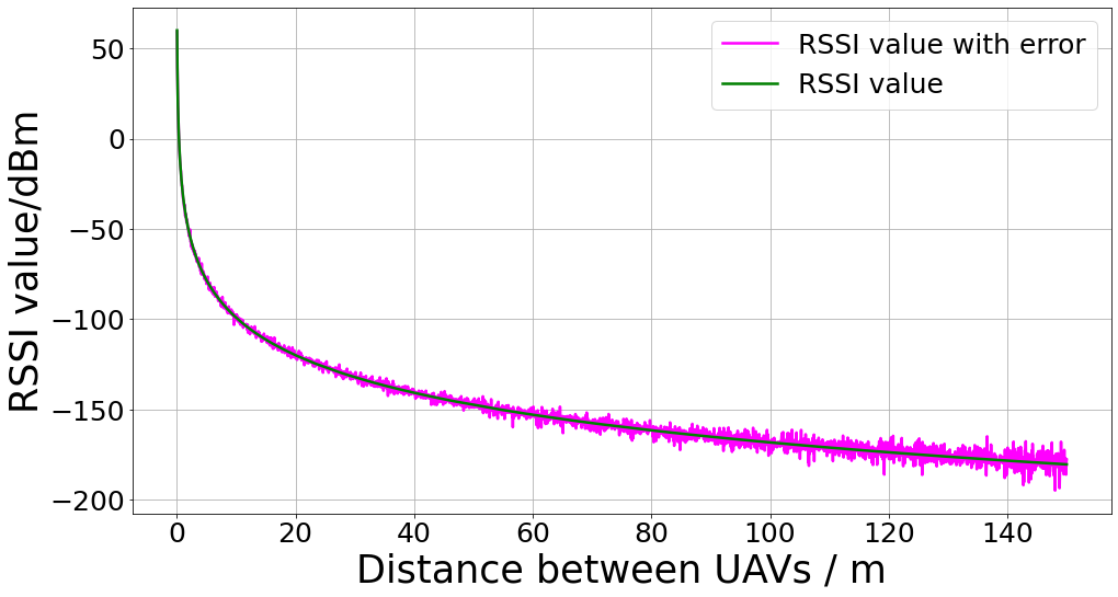
Figure 1: Simulated RSSI value over distance

By applying error to $P_{\mathrm{r}}(\textit{d})$ and find the corresponding distance of errored RSSI value, we are able to estimate the distance error $\mathcal{E}(\textit{d})$ over the distance, simulation results are presented in Fig. 2

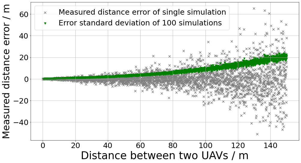
Figure 2: Estimation error and standard deviation over distance between 2 UAV s

The simulation results shows that distance estimation error $\mathcal{E}(\textit{d})$ is zero mean Gaussian distributed with $\mathcal{E}(\textit{d})\sim(0,\sigma_{\textit{d}}^{2}(\textit{d}))$, while $\sigma_{\textit{d}}(\textit{d})$ fluctuates but increases over the distance. However, based on the simulation results, distance estimation over $150$ can be extremely unreliable. Additionally, the communication cost can be drastically increased as more anchor UAV s are exposed to the target UAV.

II-B Position measurement error

For a set of anchor UAV s $\mathcal{U}=\{u_{0},u_{1},\dots u_{\mathrm{n}}\}$, each UAV has an error of its position, typically caused by various factors. With the assumption that the GPS module of UAV mitigated many of these error factors, we limited the GPS error to the Gussian error caused by the measurement. The actual position $\mathrm{p}_{n}(t)$ and its pseudo position $\mathrm{p^{\circ}}_{n}(t)$ at time step $t$ of the $n_{\mathrm{th}}$ UAV can be described :

$$\mathrm{p}_{n}(t)=[x_{n}(t),y_{n}(t),z_{n}(t)]$$ (5)

$$\mathrm{p^{\circ}}_{n}(t)=\mathrm{p}_{n}(t)+[x_{n}^{\Delta}(t),y_{n}^{\Delta}(t),z_{n}^{\Delta}(t)]$$ (6)

$$[x_{n}^{\Delta}(t),y_{n}^{\Delta}(t),z_{n}^{\Delta}(t)]\sim\mathcal{N}^{2}\left(0,\sigma_{\mathrm{p},n}^{2}/3\right)$$ (7)

$$\sigma_{\mathrm{p},n}\sim\mathcal{U}\left(\sigma_{\mathrm{min}}^{p},\sigma_{\mathrm{max}}^{p}\right)$$ (8)

where $[x_{n}^{\Delta}(t),y_{n}^{\Delta}(t),z_{n}^{\Delta}(t)]$ is position measurement error, which can be described by a zero mean Gaussian distribution with standard deviation $\sigma_{\mathrm{p},n}$. $\sigma_{\mathrm{p},n}$ is considered to be random uniform distributed. Within a valid coverage of mutual localization, a target UAV $u_{k}\in\mathcal{U}$ measures the distance from anchor UAV s. The real distance $\textit{d}_{k,n}$ and measured distance $\textit{d}^{\circ}_{k,n}$ can be described as follows :

$${d}_{k,n}=\left\|\mathrm{p}_{k}(t)-\mathrm{p}_{n}(t)\right\|$$ (9)

$$d^{\circ}_{k,n}={d}_{k,n}+{\mathcal{E}({d}_{k,n},t)}$$ (10)

III Adaptive and robust mutual localization

III-A Introduction to different localization techniques

Thorough studies have been conducted focusing on distance-based localization techniques. We focus on 3 different localization techniques: least square (LS) based localization, $l$1 norm (LN-1) based localization, and gradient descend (GD) based localization, to investigate their localization performance in the presence of uneven spatial distribution of anchor UAV s. These techniques have been widely recognized for their robustness and efficiency in sensor network scenarios [5][11].

Given the measured distance ${d}^{\circ}_{k,n}$ of anchor UAV s and their positions $\mathrm{p^{\circ}}_{n}$, the position of $u_{k}$ can be estimated by minimizing the error between measured distance and calculated distance, as described follows:

$$\begin{split}{\mathrm{p}}_{k}&=\arg\min\limits_{[x,y,z]}\sum_{n=0}^{N}\left|\|\mathrm{p^{\circ}}_{n}-{\mathrm{p}}_{k}\|-{d}^{\circ}_{k,n}\right|.\\ \end{split}$$ (11)

This optimization problem can be directly solved by LS technique with,

$$[x_{k},y_{k},z_{k},\|\mathrm{p}_{k}\|^{2}]^{\mathrm{T}}=\mathrm{(A^{T}A)^{-1}Ab}$$ (12)

where $\mathrm{A}$ and $\mathrm{b}$ are matrices containing anchor position and measured distances information,

$$A=\begin{Bmatrix}-2x_{0}\kern-6.0pt&-2y_{0}\kern-6.0pt&-2z_{0}\kern-6.0pt&1\\ \vdots\kern-6.0pt&\vdots\kern-6.0pt&\vdots\kern-6.0pt&1\\ -2x_{n}\kern-6.0pt&-2y_{n}\kern-6.0pt&-2z_{n}\kern-6.0pt&1\\ \end{Bmatrix}\mathrm{b}=\begin{Bmatrix}{{d}^{\circ}}^{2}_{k,0}-\|\mathrm{p}^{\circ}_{0}\|^{2}\\ \vdots\\ {{d}^{\circ}}^{2}_{k,n}-\|\mathrm{p}^{\circ}_{n}\|^{2}\\ \end{Bmatrix}$$

Moreover, such a localization problem can be formulated as a plane fitting problem, where the objective is to find a 4D plane $W=f(x,y,z)$ that fits the measurements $\mathrm{A}$ and $\mathrm{b}$. The coefficients of the plane can be represented as $u=[x_{k},y_{k},z_{k},\|\mathrm{p}_{k}\|^{2}]^{\mathrm{T}}$. The optimization can be performed by minimizing the $l$1 norm-based distance metric [5].

$$\begin{split}&\min\limits_{u,w}\|w\|_{1}\\ &\text{subject to }\mathrm{A}u-w=\mathrm{b}\end{split}$$ (13)

And $u$ can be solved iteratively by using Alternating Direction Method of Multiplier (ADMM) steps,

$$\begin{split}u^{i}&=\mathrm{GA^{T}}(b+u^{i-1}-\frac{\lambda^{i-1}}{\rho})\\ w_{k}&=S_{\frac{1}{\rho}}(\mathrm{A}u^{i-1}-b+\frac{\lambda^{i-1}}{\rho})\\ \lambda^{i}&=\lambda^{i-1}+\rho(\mathrm{A}u^{i}-w^{i}-b)\end{split}$$ (14)

where $\mathrm{G=(A^{T}A)}^{-1}$, $\lambda$ is the Lagrange multiplier and $\rho$ is the penalty parameter for violating the linear constraint. Meanwhile, $S_{\frac{1}{\rho}}$ is the soft threshold function in $l1$ norm, defined as $S_{\frac{1}{\rho}}=\mathrm{sign}(x)*\max({|x|-\frac{1}{\rho}},0)$.

Eq. 11 can be also reformulated as $\mathrm{p}_{k}=\arg\min\limits_{[x,y,z]}f(x,y,z)$. By applying gradient descent to cost function $f(x,y,z)$, we are able to estimate the position $\hat{\mathrm{p}}_{k}$ of $u_{k}$ iteratively. At the $i_{\mathrm{th}}$ iteration, the negative gradient $g^{i}$ and position $\hat{\mathrm{p}}_{k}$ can be calculated,

$$g^{i}=-\nabla_{(x,y,z)}(f(x,y,z))|_{(x=\hat{x}_{k}^{i-1},y=\hat{y}_{k}^{i-1},z=\hat{z}_{k}^{i-1})}$$ (15)

$$\hat{\mathrm{p}}^{i}_{k}=\hat{\mathrm{p}}^{i-1}_{k}+\alpha^{i}\times\frac{g^{i}}{||g^{i}||}$$ (16)

where $\hat{\mathrm{p}}^{i-1}_{k}$ is the estimated position at the $(i-1)_{th}$ iteration. $\alpha^{i}$ is the step size at the $i_{th}$ iteration. $\alpha^{i}$ can be adjusted by discount factor $\beta$ to prevent over-descending.

The computational complexity of the three above-introduced techniques is summarized in Tab. I [5].

TABLE I: Computational complexity

LS	LN-1	GD
$\mathcal{O}(N^{2})$	$\mathcal{O}(\max(K_{\mathrm{ADMM}}N,N^{2}))$	$\mathcal{O}(K_{\mathrm{GD}}N)$

III-B Performance evaluation under uneven spatial distribution

For UAV applications, energy consumption is a critical concern. To compare the LS, LN-1, and GD localization techniques under energy-limited conditions, we set $K_{\mathrm{ADMM}}=N$ and $K_{\mathrm{GD}}=N$ to ensure equal computational complexity for all three approaches. In the simulation, the target UAV $u_{k}$ is surrounded by anchor UAV s distributed within a cubic area. The shape of this cubic area varies, ranging from $[x_{k}\pm 35.35,y_{k}\pm 35.35,z_{k}\pm 1]$ to $[x_{k}\pm 29.29,y_{k}\pm 29.29,z_{k}\pm 28]$ to keep a maximum $d_{k,n}=50$. The RSSI error model configured as shown in Fig. 1, and simulation is set up as follows: $N=30$, $[\sigma_{\mathrm{min}}^{p},\sigma_{\mathrm{max}}^{p}]=[0.1,3]$ and $\rho=0.1$, $[\alpha^{0},\beta]=[1,0.5]$. Each estimation was repeated 50 times to exclude randomness. The results are presented in Fig. 3.

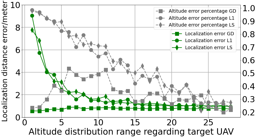
Figure 3: Localization error over spatial distribution

The simulation results show that the error of LS based and LN-1 based localization decreases as the distribution of anchor UAV s becomes more even in terms of latitude, longitude, and altitude. However, the error in GD based localization is not significantly affected by the distribution of anchor UAV s. Specifically, when anchor UAV s are densely distributed in one dimension compared to the other two dimensions, LS and LN-1 localization techniques can become highly unreliable in the densely distributed dimension. In contrast, GD based localization doesn’t show a strong correlation with the distribution of anchor UAV s in this regard. In summary, GD based localization is better suited for scenarios involving multiple UAV s, where the distribution of UAV s may be uneven in all three dimensions.

III-C Weighted localization and error conversion

To speed up the convergence of gradient descent and ensure the stability of localization, a weighted localization approach can be proposed, as described below:

$$\begin{split}\hat{\mathrm{p}}_{k}&=\arg\min\limits_{[x,y]}\sum_{n=0}^{N}\left|\|\mathrm{p}^{\circ}_{n}-\mathrm{p}\|-{d}^{\circ}_{k,n}\right|*w_{n}^{e}\end{split}$$ (17)

where $w_{n}^{e}$ is the error weight of anchor UAV s, which can be determined by the distance estimate error $\mathcal{E}$ and position measurement error power $\sigma_{\mathrm{p},n}$. To calculate the error weight, we can convert the position measurement error to the distance estimate error, as illustrated in Fig. 4.

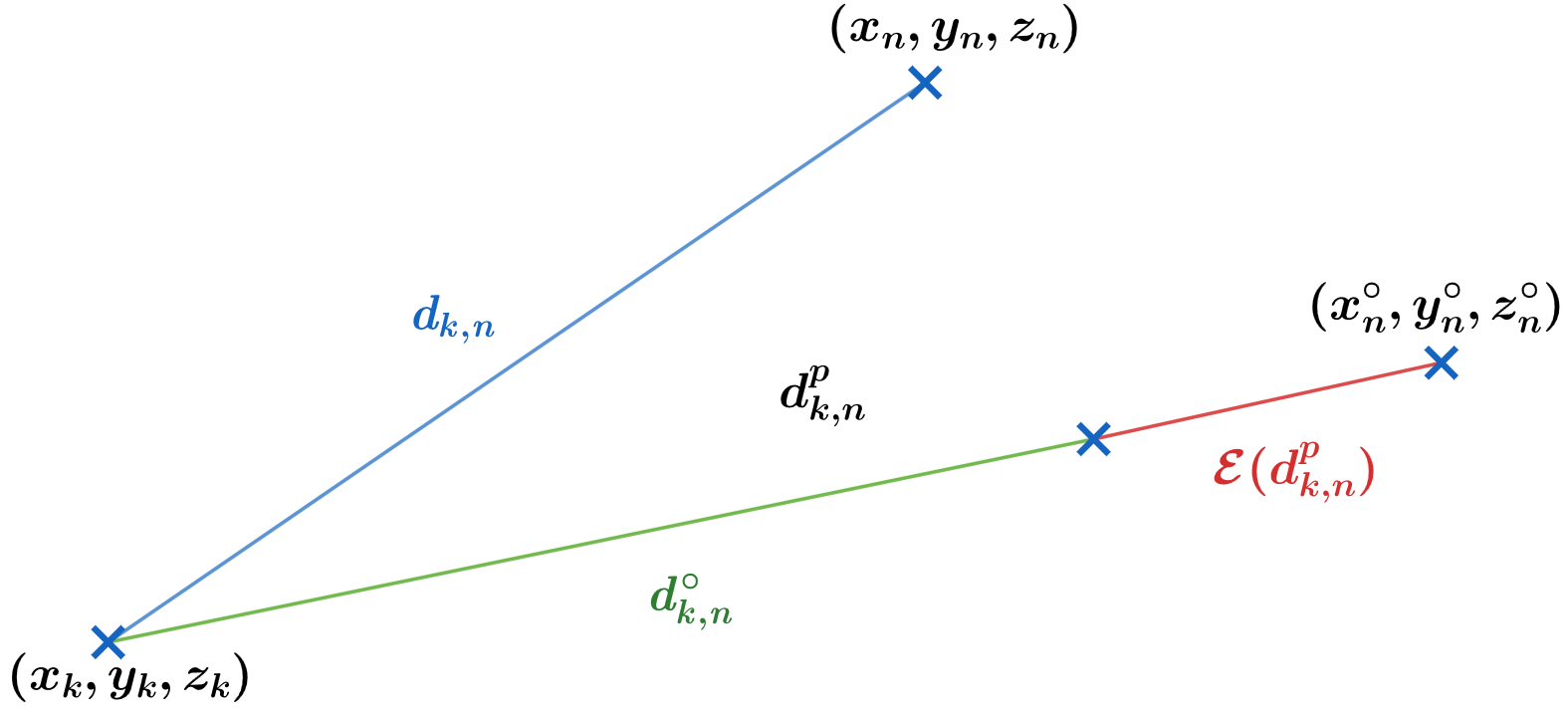
Figure 4: Position and distance estimation error conversion

For an anchor UAV $u_{n}$ with actual position $[x_{n},y_{n},z_{n}]$ and measured position $[x^{\circ}_{n},y^{\circ}_{n},z^{\circ}_{n}]$, $d_{k,n}$ is the actual distance and $d^{\circ}_{k,n}$ is the measured distance. $d^{p}_{k,n}$ is the erred distance solely caused by position error. $\mathrm{\mathcal{E}}(d^{p}_{k,n})$ is the converted distance estimation error jointly caused by position measurement and distance estimate. $\mathrm{\mathcal{E}}(d^{p}_{k,n})$ can be approximated by a non-zero mean Gaussian distribution, as introduced in [12]. Such converted distance estimate error can described as $\mathrm{\mathcal{E}}_{cd}\sim\mathcal{N}(\mu_{\mathrm{cd}},\sigma_{\mathrm{cd}})$. Nevertheless, $\sigma_{\mathrm{d}}(d_{k,n})$ can’t be directly retrieved with a single measurement of $d^{\circ}_{k,n}$. With the approximation $\sigma_{\mathrm{d}}(d_{k,n})\leftarrow\sigma_{\mathrm{d}}(d^{\circ}_{k,n})$, $d^{\circ}_{k,n}\leftarrow d_{k,n}+\mu_{cd}$ and known $\sigma_{\mathrm{p},n}$, $[\mu_{\mathrm{cd}},\sigma_{\mathrm{cd}}]$ can be obtained through least squares estimation. Error weight can be calculated as $w_{n}^{e}=\frac{\sum\limits_{u_{n}\in\mathcal{U}}\sigma_{\mathrm{c},n}}{n*\sigma_{\mathrm{c},n}}$.

III-D Mobility adaptive gradient descent Algorithm

An appropriate initial step size $\alpha^{0}$ is crucial for gradient descent-based estimation. Conventional approaches with fixed initial step sizes may not perform optimally in our scenario. To tackle this issue, we can use adaptive step sizes that dynamically adjust at each stage based on the changing speed of the target UAV $u_{k}$ and the availability of anchor UAV s.

1 Input: $\hat{\mathrm{p}}(0)=\hat{\mathrm{p}}_{init}$; discount factor $\beta_{1}$ and $\beta_{2}$; step size threshold $\epsilon^{\mathrm{max}}_{\mathrm{t_{0}}}$, $\epsilon^{\mathrm{min}}_{\mathrm{t_{0}}}$; maximum iteration, convergence threshold and momentum: $K,\theta,m$; Simulation time T

2Output: $\hat{\mathrm{p}}(t)$

3 Function MAGD$(t=1:T)$ is

4       if $t=1$ then

5            $\hat{\alpha}\leftarrow\max(\frac{\epsilon^{\mathrm{max}}_{\mathrm{t_{0}}}}{n},\epsilon^{\mathrm{min}}_{\mathrm{t_{0}}})$

6      

7      update: $\hat{\mathrm{p}}\leftarrow\hat{\mathrm{p}}(t-1);\bar{D}_{0}\leftarrow+\infty$

8      for $i=1:I$  do

9             for $n=1:N$ do

10                  get $\mathrm{p}_{n}^{\circ},\sigma_{\mathrm{p},n},d^{\circ}_{n}$ from $u_{n}$

                  get $\mu_{\mathrm{c},n},\sigma_{\mathrm{c},n}$

                    // Error conversion

11                  

                  $w_{n}^{e}\leftarrow\frac{\sum\limits_{u_{n}\in\mathcal{U}}\sigma_{\mathrm{c},n}}{n*\sigma_{\mathrm{c},n}}$

                    // Calculate error weight

12                  

13                  $\hat{d}_{n}=\|\hat{\mathrm{p}}-\mathrm{p}_{n}^{\circ}\|$

14            

            $G^{i}\leftarrow\sum\limits_{u_{n}\in\mathcal{U}}\frac{(\hat{\mathrm{p}}-\mathrm{p}^{\circ}_{n})*w_{n}^{e}}{\hat{d}_{n}}*(\hat{d}_{n}-d^{\circ}_{n}+\mu_{c,n})$

              // Gradient

15            

16            update: $\hat{\mathrm{p}}\leftarrow\hat{\mathrm{p}}+m*\hat{\mathrm{p}}+\frac{\hat{\alpha}}{n}*\frac{G^{i}}{\|G^{i}\|}$; $\hat{d}_{n}$ $\bar{D}_{i}\leftarrow\frac{1}{n}*\sum\limits_{u_{n}\in\mathcal{U}}(\hat{d}_{n}-d^{\circ}_{n}+\mu_{c,n})*w_{n}^{e}$

17            if $\bar{D}_{i}>\bar{D}_{i-1}$ then

                   $\hat{\alpha}\leftarrow\hat{\alpha}*\beta_{1}$

                    // reduce step size

18                  

19            else if $\frac{\bar{D}_{i-1}-\bar{D}_{i}}{\bar{D}_{i}}<=\theta$ then

20                  break

21            

22      update: $\hat{\mathrm{p}}(t)\leftarrow\hat{\mathrm{p}};\bar{D}(t)\leftarrow\bar{D}_{i}$;

      $V(t)\leftarrow\|\hat{\mathrm{p}}(t)-\hat{\mathrm{p}}(t-1)\|$

        // Estimate speed

23      

      $\bar{V}\leftarrow\frac{1}{t}\sum\limits_{t=1}^{t}V(t)$

        // Estimated average speed

24      

      $\bar{\bar{D}}\leftarrow\frac{1}{t}\sum\limits_{t=1}^{t}D(t)$

        // Average distance difference

25      

26      if $t<\Phi$ then

27            $\phi=t$

28      

29      else if $t>=\Phi$ then

30            $\phi=\Phi$

31      

      $\rho_{D}\leftarrow\frac{\sum\limits_{t=t-\phi}^{t}\bar{D}(t)}{(t=t-\phi)*\bar{D}}$

        // Apply smooth window

32      

33      $\rho_{V}\leftarrow\frac{\sum\limits_{t=t-\phi}^{t}V(t)}{(t=t-\phi)*\bar{V}}$

      $\rho\leftarrow\sqrt{\frac{\rho_{D}}{\rho_{V}}}$

        // Modification factor

34      

35      if $t\neq 1\And\frac{|\bar{D}(t)-\bar{\bar{D}}|}{\bar{\bar{D}}}<=0.5$ then

             $\hat{\alpha}\leftarrow\hat{\alpha}-\beta_{2}*\bar{V}$

              // Reduce step size

36            

37            $\hat{\alpha}\leftarrow\max(\hat{\alpha},\max(\frac{\epsilon^{\mathrm{min}}_{\mathrm{t}}}{n},\frac{\bar{V}}{2}))$

38      if $t\neq 1\And\rho>1.5$ then

39            

            $\hat{\alpha}\leftarrow\hat{\alpha}*{\rho}$

              // Enlarge step size

40            

41      

Algorithm III.1 Mobility adaptive gradient descend algorithm

A mobility adaptive gradient descent algorithm can be designed, as shown in Alg III.1. Step size is initialized in lines 5-6 with the given thresholds ($\epsilon^{\mathrm{max}}_{\mathrm{t_{0}}}$ and $\epsilon^{\mathrm{min}}_{\mathrm{t_{0}}}$) at the beginning. As the localization error is initially large, a larger $\hat{\alpha}$ is used for stability. Lines 7-18 perform a gradient descent-based estimation using the previous position estimate (to guarantee a good convergence within $K$) and information from anchor UAV s. Momentum $m$ stabilizes gradient descent, while discount factor $\beta_{1}$ reduces step size within each estimation. $\bar{D}_{i}$ represents the average distance difference between $\hat{d}_{n}$ and $d^{\circ}_{n}$, serving as an indicator of over-descending. Convergence threshold $\theta_{t}$ and max iteration threshold $K$ are used to terminate iterations. Lines 21-23 estimate current speed $V(t)$, average speed $\bar{V}$, and average distance difference $\bar{\bar{D}}$. The current distance difference $\bar{D}(t)$ can deviate due to occasional mis-localization, but a consistently enlarging $\bar{D}(t)$ suggests a small $\hat{\alpha}$, which results in a gradual loss of position accuracy. When $\hat{\alpha}$ is small, $\mathrm{p}(t)$ remains close to the previous estimate, resulting in a small estimated $V(t)$. In lines 27-29, a smoothing window of length $\phi$ is applied to the estimates to mitigate fluctuations, and a modification factor $\rho$ is determined conjunctively by $V(t)$ and $\bar{D(t)}$ to modify $\bar{\alpha}$. Lines 24-28 adapt the learning rate based on stability and speed. When the position estimation is stable (indicated by $\bar{D}(t)$ shows no significant deviation), $\hat{\alpha}$ is reduced by $\beta_{2}$ and $\bar{V}$ to ensure good accuracy. The minimum threshold of $\hat{\alpha}$ is determined by $\epsilon^{\mathrm{min}}_{\mathrm{t_{0}}}$ and $\bar{V}$. If the estimation is not stable, $\hat{\alpha}$ is increased by $\rho$.

III-E Accuracy estimation of mutual localization system

We access the robustness and accuracy of MAGD through simulations with varying numbers of anchor UAV s and fixed step sizes, and then compare the simulation results based on MAGD. The movement speed of $u_{k}$ is periodically changed to simulate real mobility. Anchor UAV s $u_{n}$ are randomly initialized within a cubic area around target UAV $u_{k}$. The system configuration is summarized in Tab II.

TABLE II: Simulation Setup 1

	Parameter	Value	Remark
	$n_{a}$	$5\sim 40$	Anchor UAV s
	$\sigma^{2}_{\mathrm{p},n}$	$\sim\mathcal{U}(0.1,3.0)$	Position error power / $\mathrm{m}^{2}$
	$V$	$\sim\mathcal{U}(0.6,3.4)$	Travel speed $\mathrm{m}\mathrm{/}\mathrm{s}$
	$T$	50 s	Simulation time
System	$[\epsilon^{\mathrm{max}}_{\mathrm{t_{0}}},\epsilon^{\mathrm{min}}_{\mathrm{t_{0}}}]$	[50,5]	Step size thresholds
	$[\beta_{1},\beta_{2}]$	$[0.5,0.05]$	Discount factors
	$m$	$1\times 10^{-5}$	Momentum
	$\theta$	$1\times 10^{-8}$	Convergence threshold
MGAD	$K$	30	Maximum iteration

The simulation results in Fig 5 depict the average error of 50 estimates. Among the three best fixed step sizes, $\alpha=(1.5,2.3,2.7)$ yield average localization errors across all $n_{a}$ of $(1.63,1.67,1.66)$ respectively. In comparison, the average localization error archived by MAGD in this regard is 1.47, indicating that MAGD outperforms conventional approaches with fixed $\alpha^{0}$. In this specific setup, step sizes ranging from 1.4 to 3.0 show robust performance, although such a range may be challenging to find in practice. By adjusting $\alpha^{0}$ to different scenarios, our proposed method efficiently provides robust position estimation with good accuracy.

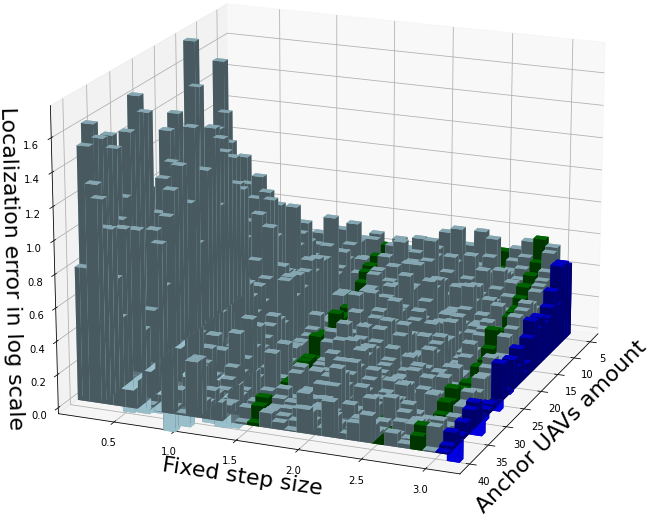
Figure 5: Localization error of fixed step sizes and MAGD (3 best step sizes are marked in green and MAGD in darkblue)

IV Attack Paradigm and mutual attack detection system

IV-A Attack Paradigm

Potential attacks on localization techniques can be categorized into several aspects.

Jamming mode: the attacker jams the beacon signal of $u_{n}$ to introduce large distance estimation error and induce a wrongly received $\mathrm{p}(n)$ and $\sigma_{\mathrm{p},n}$. The received signal can be represented as $[\mathrm{p}^{\circ}_{n}+\mathrm{\tilde{p}}_{n},({d}^{\circ}_{k,n}+\tilde{d}_{k,n})^{+},\sigma_{\mathrm{p},n}+\tilde{\sigma}_{\mathrm{J}}]$. Take the simplification, $\mathrm{\tilde{p}}_{n}\sim\mathcal{N}^{3}\left(0,\tilde{\sigma}_{\mathrm{J}}^{2}/3\right)$, $\tilde{d}_{k,n}\sim\mathcal{U}\left(0,\tilde{\sigma}_{\mathrm{J}}^{2}\right)$, where $\tilde{\sigma}^{2}_{\mathrm{J}}$ is the jamming index. Bias mode: the attacker hijacks some of the UAV s to erroneously report its position with a certain position bias to mislead others. In this scenario, the received signal can be modeled as $[\mathrm{p}^{\circ}_{n}+\tilde{\mathrm{B}},{d}^{\circ}_{k,n},\sigma_{\mathrm{p},n}]$, where $\tilde{\mathrm{B}}$ denotes position bias. Manipulation mode: the attacker hijacks some of the UAV s to report its position with an extra error, simultaneously modify its $\sigma_{\mathrm{p},n}$ to be extremely small for the intention of manipulating $w_{n}^{e}$. The received signal can be concluded as $[\mathrm{p}^{\circ}_{n}+\mathrm{\tilde{p}}_{n},{d}^{\circ}_{k,n},1/\tilde{\sigma}_{\mathrm{M}}]$, where $\mathrm{\tilde{p}}_{n}\sim\mathcal{U}\left(0,\tilde{\sigma}^{2}_{\mathrm{M}}/3\right)$, $\tilde{\sigma}^{2}_{\mathrm{M}}$ is the manipulation index.

In a constantly moving scenario, attack strategies can be categorized as follows. Global random attack: All malicious UAV s are uniformly distributed and randomly attack all nearby UAV s. This strategy aims to degrade position estimation globally and penetrate existing attack detection systems, as suggested in [13]. Global coordinated attack: Similar to the global random attack, the malicious UAV s coordinate their attacks within a certain time frame. Stalking strategy: All malicious UAV s follow a victim UAV and constantly attack it. This strategy does not impact estimation accuracy globally but targets the victim specifically.

IV-B Anomaly detection and trust propagation mechanism

Considering the above-mentioned attack schemes, a robust attack detection algorithm should be degrading the trustworthiness of suspicious UAV s. To achieve this, a reputation weight $r_{n}$ can be applied in MAGD, more specifically in Alg III.1 line 13 and 15,

$$G^{i}\leftarrow\sum\limits_{u_{n}\in\mathcal{U}}\frac{(\hat{\mathrm{p}}-\mathrm{p}_{n})*w_{n}^{e}*r_{n}}{d_{n}}*(d_{n}-d^{\circ}_{n})$$ (18)

$$\bar{D}_{i}\leftarrow\frac{1}{n}*\sum\limits_{u_{n}\in\mathcal{U}}(\hat{d}_{n}-d^{\circ}_{n}+\mu_{c,n})*w_{n}^{e}*r_{n}$$ (19)

Our proposed method, illustrated in Alg IV.1, estimates reputation weight using the cumulative distribution function of $\mathcal{N}(\mu_{\mathrm{cd},n},\sigma_{\mathrm{cd},n})$. In lines 7-8, $u_{k}$ calculates the estimated distance error $\hat{\mathrm{\mathcal{E}}}_{n}$ based on information from $u_{n}$ and the converted error distribution. Lines 12-16 address potential manipulation attacks by limiting $\sigma_{\mathrm{c},n}$ to a predefined minimum position error power $\sigma_{\mathrm{p},\min}$. Then compare the cumulative density $\xi_{n}$ with a preset probability threshold $\epsilon^{t}$ to detect the attack behavior of $u_{n}$. Depending on the detection results, the reputation weight update is performed with a punishment or reward $[\lambda_{r},\lambda_{p}]$. The updated $r_{n}(t)$ considers its previous value $r_{n}(t-1)$, a forget factor $\gamma$, and the corresponding reward or penalty. Then $r_{n}(t)$ is thresholded within the range of [0,1]. This approach aims at countering coordinated attacks, allowing $r_{n}(t)$ to recover gradually when attacks from $u_{n}$ become less frequent, without compromising mutual localization accuracy.

1 Input: Reward $\lambda_{r}$ and penalty $\lambda_{p}$, forget factor $\gamma$ and confidence threshold $\epsilon^{t}$

2 Output: $r_{n}(t)$

3Initialize: $r_{n}(t=1)\leftarrow 1$

4 Function TAD$(t=1:T)$ is

5       get $\hat{\mathrm{p}}(t)$ from MAGD$(t)$ meanwhile apply $r_{n}(t-1)$

6       for $n=1:N$ do

7            get $\sigma_{\mathrm{p},n},d^{\circ}_{n},\mathrm{p}^{\circ}_{n}$ from $u_{n}$

8            get $\mu_{\mathrm{c},n},\sigma_{\mathrm{c},n}$

9            $\hat{d}_{n}\leftarrow\|\hat{\mathrm{p}}-\mathrm{p}_{n}\|$

            $\hat{\mathrm{\mathcal{E}}}_{n}\leftarrow|\hat{d}_{n}-d^{\circ}n+\mu_{\mathrm{cd}}|$

              // Distance error of $u_{n}$

10            

11            calculate CDF $\xi_{n}$,

12            $\sigma_{\mathrm{c},n}\leftarrow\max(\sigma_{\mathrm{c},n},\sigma_{\mathrm{p},min})$

13             $\xi_{n}\leftarrow P_{\hat{\mathrm{\mathcal{E}}}_{n}}\left[\hat{\mathrm{\mathcal{E}}}_{n}~{}|~{}\mu_{\mathrm{c},n},(\sigma_{\mathrm{c},n})^{2}\right]$

14            if $\xi_{n}>\epsilon^{t}$ then

15                  

                  $\hat{r}_{n}\leftarrow\lambda_{r}$

                    // Assign reward

16                  

17            else

18                  

                  $\hat{r}_{n}\leftarrow\lambda_{p}$

                    // Assign penalty

19                  

20            

21            update $r_{n}(t)$

22            $r_{n}(t)\leftarrow\gamma*[r_{n}(t-1)+1]-1+\hat{r}_{n}$

23            $r_{n}(t)\leftarrow\min(1,\max(0,r_{n}(t))$

24      

Algorithm IV.1 Time-evolving anomaly detection

To address the vulnerability of target UAV s to spatial ”ambushing” or stalking attacks, we incorporate a global reputation system. This system allows UAV s to share their local reputations with each other. Nevertheless, malicious reputation information can be shared as well, therefore a reputation propagation scheme is implemented. This ensures that reputation weights are carefully propagated, maintaining the reliability and accuracy of reputation information within the system. The propagated reputation weights can be described as follows:

$$\tilde{r}_{k,n}=\frac{\sum\limits_{m\notin{k,n}}{r}_{k,m}*{r}_{m,n}}{\sum\limits_{m\notin{k,n}}{r}_{k,m}},\tilde{\tilde{r}}_{k,n}=\frac{\mathrm{F_{p}}(\tilde{r}_{k,n})+{r}_{k,n}}{2}.$$ (20)

While $u_{k}$ is utilizing the mutual localization system, $u_{1}...u_{n}$ are the accessible anchor UAV s, and ${r}_{k,n}$ is the local reputation. $u_{m}$ has uploaded its local reputation to the cloud, enabling reputation ${r}_{m,n}$ from $u_{m}$ to $u_{n}$ to be accessed. Meanwhile, $u_{k}$ has a local reputation ${r}_{k,m}$ to $u_{m}$. Based on the local reputation ${r}_{k,m}$, the uploaded reputation will be discriminated against accordingly. A propagated reputation $\tilde{r}_{k,n}$ is strongly leaning to UAV which has a good reputation to $u_{k}$. $\mathrm{F_{p}}$ is the propagation function designed to discriminate the already notorious $u_{n}$(a convex function is applied). Subsequently, proceed with the mean of local reputation and propagated reputation to MAGD.

V Simulation results

V-A Evaluation under different attack mode and strategy

TABLE III: Simulation Setup 2

	Parameter	Value	Remark
	Map Size	$[300,300,10]$	Define map size
	$n$	$100$	number of anchor UAV s
	$\sigma^{2}_{\mathrm{p},n}$	$\sim\mathcal{U}(0.1,3.0)$	Position error power / $\mathrm{m}^{2}$
	$V$	$\sim\mathcal{U}(0.3,1.7)$	Travel speed $\mathrm{m}\mathrm{/}\mathrm{s}$
	$T$	100 s	Simulation time
MGAD	$m$	$1\times 10^{-5}$	Momentum
	$\theta$	$1\times 10^{-8}$	Convergence threshold
	$K$	30	Maximum iteration
	$[\lambda_{r},\lambda_{p}]$	$[0.3,-0.7]$	Reward and penalty
	$\gamma$	$0.5$	Forget factor
	$\epsilon^{t}$	$0.95$	Confidence threshold
TAD	$n_{m}$	$30$	Malicious UAV s
	$r_{a}$	$0.5$	Attack rate if random attack
	$T_{a}$	$50$	Attack time frame if coordinated attack
	$\tilde{\mathrm{B}}_{n}$	$[200,200,5]$	Position bias if bias attack
	$\tilde{\sigma}^{2}_{\mathrm{M},n}$	$200$	Manipulation index if manipulation attack attack
Attacker	$\tilde{\sigma}^{2}_{\mathrm{J},n}$	$5$	Jamming index if jamming attack attack

TABLE IV: Estimate error () under different attack scheme and malicious UAV s percentage

	10-20%	20-30%	30-40%	40-50%	50-60%
No attack	1.62	–	–	–	–
No attack with TAD	1.58	–	–	–	–
Coord. Bias	3.89	7.29	10.80	12.84	19.54
Coord. Bias with TAD	1.72	1.88	2.05	2.06	4.25
Random Bias	1.82	1.84	1.73	1.68	1.74
Random Bias with TAD	1.64	1.66	1.62	1.74	1.74
Coord. Mani.	2.05	2.32	2.58	4.63	2.82
Coord. Mani. with TAD	1.72	1.86	1.88	2.16	2.71
Random Mani.	1.77	1.57	1.54	1.68	1.66
Random Mani. with TAD	1.58	1.71	1.61	1.56	1.71
Coord. Jam.	1.97	2.06	2.24	2.18	2.39
Coord. Jam. with TAD	1.94	2.03	2.03	2.28	2.43
Random Jam.	1.95	1.93	2.12	2.16	2.19
Random Jam. with TAD	1.95	2.04	1.62	1.72	1.68

To validate the robustness and effectiveness of TAD, we carried out simulations of our mutual localization system under different attack modes and strategies, while 10 targets $u_{k}$ navigates through attackers. We assume the attacker has limited resources and can only jam/hijack some part of the UAV s. The attacks can be organized as random or coordinated. The MAGD configuration follows Tab.II, while system, TAD and attacker parameters are listed in Tab.III. The attack rate and attack time frame are set to 0.5 and 50 to keep an unvarying attack power. All anchor UAV s are distributed within the map and navigate to random destinations, which leads to an average of 15 anchor UAV s within a mutual localization range of $50$. Target UAV s can be anchor UAV s to each other, $\sigma^{2}_{\mathrm{p},k}$ is set to be $\max(\sigma^{2}_{\mathrm{p},n})$. The simulation results are shown in Fig. 6 and Tab. IV.

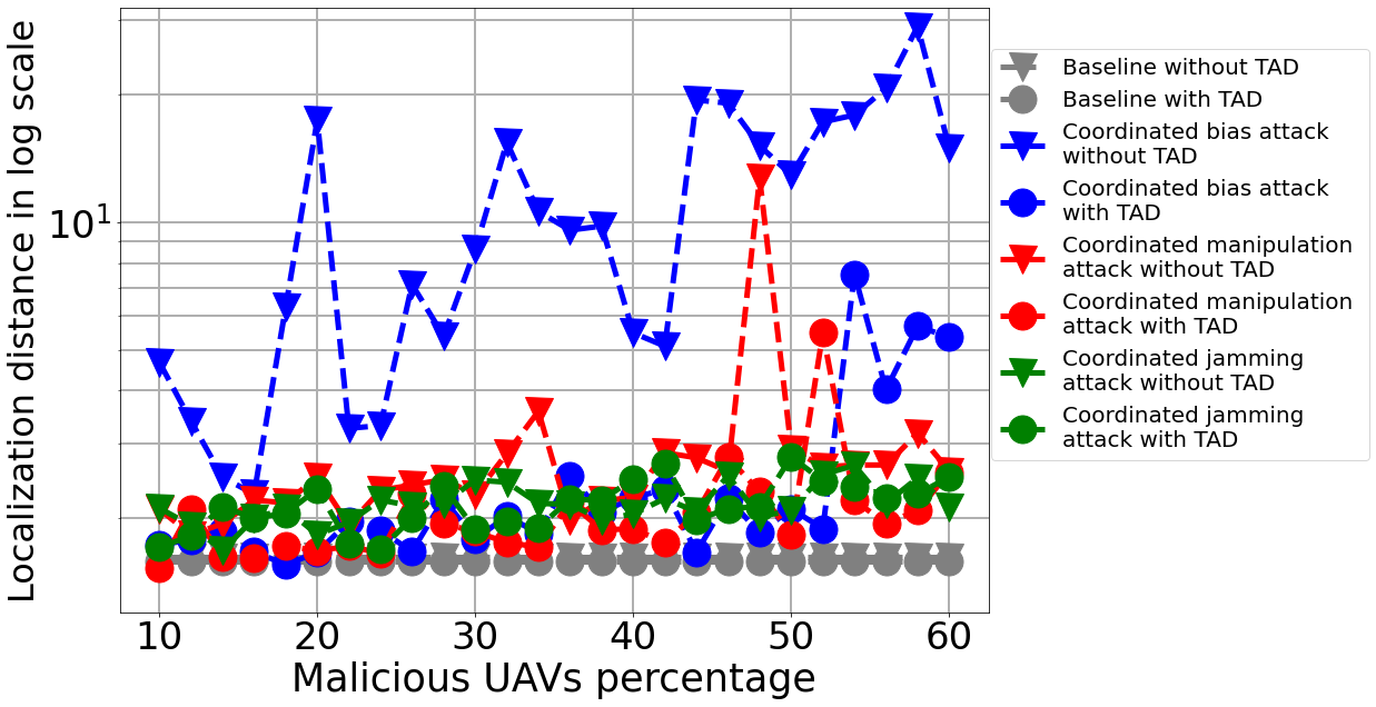
(a) Coordinated attack scheme

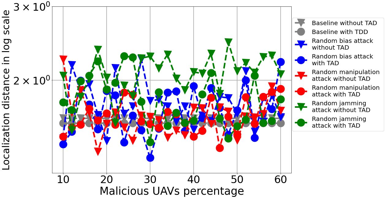
(b) Random attack scheme

Figure 6: Localization error of different over malicious UAV s percentage

Contrary to findings in static sensor networks, our results indicate that coordinated attacks are more effective than uncoordinated ones, contradicting the suggestion that both schemes are equally effective [14][5]. The inconsistency in error injection during each MAGD’s gradient descent process leads to this difference. MAGD can still provide accurate estimations under less dense attacks due to varying attack density, preventing a cascading effect of mislocalization caused by injected errors. Random attacks lead to temporary large localization errors, which can be quickly resolved within a few timesteps. In contrast, coordinated attacks cause sustained mis-localization (detailed trace error analysis emitted in this paper due to the length limit). Moreover, the results demonstrate that attack mode bias exhibits higher effectiveness in causing large localization errors. This is attributed to the fact that the injected errors in this mode do not offset each other, leading to a cumulative impact on the localization accuracy. Additionally, the coordinated jamming mode poses a formidable challenge to TAD as it enlarges $\sigma_{c,n}$ of malicious UAV s, which makes it challenging for TAD to identify attacks. Nonetheless, our proposed weighted localization approach effectively mitigates such attacks by favoring anchor UAV s with smaller $\sigma_{c,n}$, thereby bolstering the overall resilience and robustness of the localization system.

To further assess TAD and RP, we conducted simulations with malicious UAV s employing a coordinated stalking strategy to attack the victim target $u_{k}$. The parameters for MAGD and TAD follow those listed in Table III, while the attack mode is set to bias mode. The percentage of malicious UAV s is set at $30\%$, which includes 3 target UAV s capable of attacking other target UAV s while sharing malicious reputation. We assume the attacker knows the actual position of the victim target with ambiguity (the estimated position $\hat{\mathrm{p}}_{k}$, shared by $u_{k}$, should not be used as it can be misleading when attacks become effective). The results in Fig. 7 show average errors of 20 simulations at different time steps.

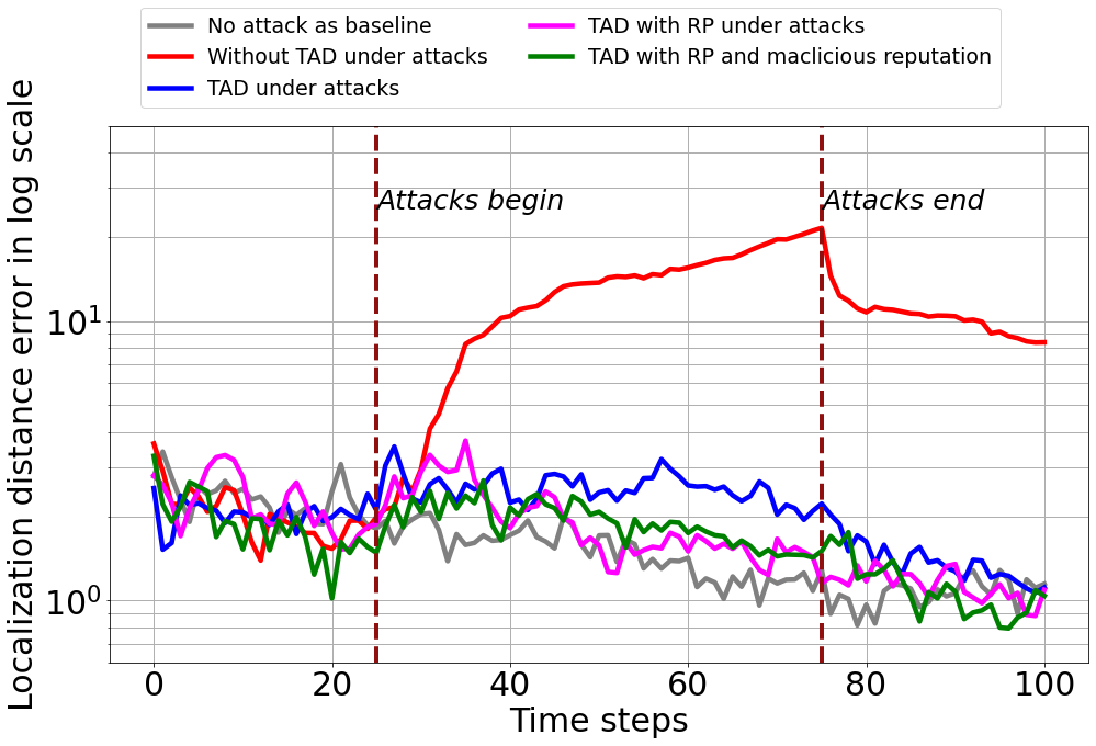
Figure 7: Localization error at different time step (for the baseline, UAVs are set to follow the target as well)

Our simulation results demonstrate the effectiveness of TAD against stalking attack strategies with the given attack density, significantly reducing localization errors compared to the absence of TAD. Moreover, the introduction of RP further enhances localization performance, leading to a faster convergence of localization errors compared to TAD alone. Notably, RP also exhibits resilience to malicious reputation information.

VI Conclusion

In this paper, we evaluated localization techniques and presented a novel localization scheme (MAGD) that adapts to the mobility and changing availability of anchor UAV s. Additionally, we introduced defense schemes (TAD and RP) to counter potential attacks. Our numerical simulations demonstrated the effectiveness of these methodologies in dynamic scenarios.

However, it is essential to acknowledge that this study did not extensively address potential attacks against RP. A sophisticated attacker might manipulate a subset of compromised UAV s to launch attacks on target UAV s while others share a malicious reputation. This poses a challenge for our TAD and RP to effectively detect and mitigate such attacks. The potential threat calls for a novel approach to identifying attack patterns.

References

- [1] Z. Feng, Z. Na, M. Xiong et al., “Multi-uav collaborative wireless communication networks for single cell edge users,” Mobile Networks and Applications, vol. 27, pp. 1–15, 01 2022.
- [2] S. Dwivedi, R. Shreevastav, F. Munier et al., “Positioning in 5g networks,” IEEE Communications Magazine, vol. 59, no. 11, pp. 38–44, 2021.
- [3] P. Krapež and M. Munih, “Anchor calibration for real-time-measurement localization systems,” IEEE Transactions on Instrumentation and Measurement, vol. 69, no. 12, pp. 9907–9917, 2020.
- [4] L. L. d. Oliveira, G. H. Eisenkraemer, E. A. Carara et al., “Mobile localization techniques for wireless sensor networks: Survey and recommendations,” ACM Trans. Sen. Netw., vol. 19, no. 2, apr 2023. [Online]. Available: https://doi.org/10.1145/3561512
- [5] B. Mukhopadhyay, S. Srirangarajan, and S. Kar, “Rss-based localization in the presence of malicious nodes in sensor networks,” IEEE Transactions on Instrumentation and Measurement, vol. 70, pp. 1–16, 2021.
- [6] S. Jha, S. Tripakis, S. Seshia et al., “Game theoretic secure localization in wireless sensor networks,” 2014 International Conference on the Internet of Things (IOT), pp. 85–90, 10 2014.
- [7] S. Tomic and M. Beko, “Detecting distance-spoofing attacks in arbitrarily-deployed wireless networks,” IEEE Transactions on Vehicular Technology, vol. 71, pp. 4383–4395, 2022.
- [8] H. Wang, J. Wan, and R. Liu, “A novel ranging method based on rssi,” Energy Procedia, vol. 12, pp. 230–235, 12 2011.
- [9] A. Fakhri, S. Gharghan, and S. Mohammed, “Path-loss modelling for wsn deployment in indoor and outdoor environments for medical applications,” International Journal of Engineering and Technology(UAE), vol. 7, pp. 1666–1671, 08 2018.
- [10] J. Allred, A. Hasan, S. Panichsakul et al., “Sensorflock: an airborne wireless sensor network of micro-air vehicles,” 11 2007, pp. 117–129.
- [11] R. Garg, A. L. Varna, and M. Wu, “An efficient gradient descent approach to secure localization in resource constrained wireless sensor networks,” IEEE Transactions on Information Forensics and Security, vol. 7, no. 2, pp. 717–730, 2012.
- [12] B. Han and H. D. Schotten, “A secure and robust approach for distance-based mutual positioning of unmanned aerial vehicles,” 2023, preprint available at arXiv:2305.12021.
- [13] B. Han, D. Krummacker, Q. Zhou et al., “Trust-awareness to secure swarm intelligence from data injection attack,” 2023, to appear at IEEE ICC 2023, preprint available at arXiv:2211.08407.
- [14] B. Mukhopadhyay, S. Srirangarajan, and S. Kar, “Robust range-based secure localization in wireless sensor networks,” 2018 IEEE Global Communications Conference, pp. 1–6, 12 2018.