Optimal strategies for mosquitoes replacement strategy: influence of the carrying capacity on spatial releases
Abstract
This work is devoted to the mathematical study of an optimization problem regarding control strategies of mosquito population in a heterogeneous environment. Mosquitoes are well known to be vectors of diseases, but, in some cases, they have a reduced vector capacity when carrying the endosymbiotic bacterium Wolbachia. We consider a mathematical model of a replacement strategy, consisting in rearing and releasing Wolbachia-infected mosquitoes to replace the wild population. We investigate the question of optimizing the release protocol to have the most effective replacement when the environment is heterogeneous. In other words we focus on the question: where to release, given an inhomogeneous environment, in order to maximize the replacement across the domain. To do so, we consider a simple scalar model in which we assume that the carrying capacity is space dependent. Then, we investigate the existence of an optimal release profile and prove some interesting properties. In particular, neglecting the mobility of mosquitoes and under some assumptions on the biological parameters, we characterize the optimal releasing strategy for a short time horizon, and provide a way to reduce to a one-dimensional optimization problem the case of a long time horizon. Our theoretical results are illustrated with several numerical simulations.
Mathematics Subject Classifications: 49K15; 49M05; 92D25
Keywords: Optimal control, spatial heterogeneity, population replacement, Wolbachia bacterium, vector control.
1 Introduction
Mosquitoes of the genus Aedes are responsible for the transmission of many diseases to humans. Among them, one may cite dengue, Zika, and chikungunya. One promising way to control the spread of such diseases is the use of the bacterium Wolbachia [10]. Indeed, it has been reported that Wolbachia-infected mosquitoes are less capable of transmitting such diseases [33, 7]. Moreover, this bacterium is characterized by, on the one hand, a vertical transmission from mother to offsprings and, on the other hand, producing a cytoplasmic incompatibility, which makes the mating of Wolbachia-infected males with wild females to be less fertile [29]. Taking advantage of these features, a population replacement strategy has been developed by rearing and releasing Wolbachia-infected mosquitoes [18]. This strategy is becoming very popular since it is potentially self-sustaining and has been successfully deployed in the field by the World Mosquito Program (see [16, 25] and https://www.worldmosquitoprogram.org/).
It has motivated several works including mathematical studies that have proved to be of great interest by proposing models that can be used to test and optimize different scenarios, see e.g. [19, 26, 3] and the review article [24]. In particular, mathematical control theory has been used to study the feasibility of the strategy, see e.g. [1, 9, 12]. A natural question is the optimisation of the release protocol. How to design the best release protocol, taking into account production constraints, to have the most efficient population replacement? Several mathematical works have addressed this issue. First, the optimisation of the temporal distribution of the releases, neglecting the spatial dependency, has been studied in e.g. [11, 6, 4, 2]. In particular, using a reduced model, the authors in [6] show that the best strategy is close to a bang-bang strategy where the maximum number of mosquitoes available is released at one time at the beginning or end (depending of the number of mosquitoes available) of the release period. Then, the study of the optimisation in space has been initiated in [5, 13, 23, 21] assuming that the space is homogeneous. In these works, the release is assumed to be done at initial time only and the question is to know how to spatially distribute the population to release in order to optimize the efficiency.
However, it is clear that for practical applications, environment cannot be considered as homogeneous and heterogeneity may have a strong influence on the dynamics of the replacement (see e.g. [22]). The aim of this paper is to propose a first mathematical study of an optimisation problem for a population replacement in a non-homogeneous landscape. More precisely, we consider the two-population model used in [6], see also [14, 15, 17, 32], where similar systems are considered, and assume that the carrying capacity of the environment is heterogeneous in space, modelling the fact that some areas are more favourable than others for the mosquito population. The system is first reduced in the spirit of [30], and the release is assumed to be pointwise in time: Indeed, it has been observed in [6, 3] that this is often the best strategy. Moreover, the spatial active motion of mosquitoes, usually modelled by a diffusion term, is neglected for the sake of simplicity. To fix the notation, let us present briefly the resulting optimisation problem considered in this article. Denote the fraction of Wolbachia-infected population at time and position , with being a bounded domain of or . We seek to minimize the distance, at some given final time , between the proportion and the total invasion constant steady state . Using the -norm, the problem reads
In this problem, is the given carrying capacity depending on the space variable , and is the initial release function which is positive, bounded by a constant and such that its integral (which corresponds to the total quantity of mosquitoes released) is bounded by . The relation between this release function and the proportion is obtained by solving the differential equation
In this system, is a given bistable function and is a given positive and increasing function. Their expressions will be given explicitly later. Solving this optimal control problem boils down to investigate the question : what is the best initial distribution of the release in a heterogeneous environment in order to optimize the population replacement when active motion of mosquitoes is neglected?
Up to our knowledge, this work is the first one considering spatial heterogeneity in such an optimisation problem. We mention that neglecting active motion of mosquitoes allows us to reduce the problem to a dynamical system instead of considering a reaction-diffusion system, which greatly simplifies the study, and allows to derive precise results on the optimum. Although the study is simplified, it is very challenging to get a precise description of the optimal solution. This is a first step towards more sophisticated and more realistic future works where the active motion of mosquitoes will be considered. However, from a numerical point of view, we may draw some comparisons between numerical solutions of models with and without diffusion and check that, in certain conditions, they have a similar behaviour (see section 4.2).
The outline of the paper is the following. In the next section, we present the modelling assumptions and introduce the optimisation problem we are considering. Then, section 3 is devoted to the theoretical analysis of the optimisation problem and to the proof of our main results. Section 4 provides some numerical illustrations of our results. We also show numerical comparisons with a more realistic model with diffusion. Finally, some technical computations are provided in an appendix.
2 Mathematical model and optimal control problem
2.1 Simplified system
Let denote a function accounting for the rate at which Wolbachia-infected mosquitoes are released in a given bounded domain, , of or . To model the dynamics of the replacement of a wild population of mosquitoes by Wolbachia-infected mosquitoes, the following system has been considered in e.g. [6]. In this system, the density of the Wolbachia-infected species is denoted , whereas the density of the wild population to be replaced is denoted . The system reads
| (2.1) |
In this system, , , and , represent the intrinsic birth and death rates of population (i.e. not considering the term representing the population limitation due to the carrying capacity). In many insect species, among which we find mosquitoes, the birth rate is considerably higher than the death rate, therefore for biological reasons we will consider the constraint . Also, we assume that the second population has a fitness disadvantage with respect to the first one, due to the infection with Wolbachia. This translates into imposing and . The parameter measures the Wolbachia-induced cytoplasmatic incompatility (CI) of the second population over the first one. We have that , when there is a perfect CI, when there is none. We assume that, at there are no Wolbachia-infected individuals and that the wild population is at equilibrium, that is and . The diffusion coefficient is denoted and the carrying capacity . In (2.1), is the time horizon of the problem. In this work we consider that the carrying capacity has Lipschitz spatial dependency:
The goal we pursue is to find an optimal release function, , such that at a given final time the solution to (2.1) is as close as possible of the -invasion steady state denoted . Choosing a least square distance, this leads us to introduce the following cost functional
| (2.2) |
We consider some natural constraints on the number of available individuals to realize the experiments and also on the rate at which this individuals can be released. The set of admissible controls is therefore given by
| (2.3) |
This is inspired by the problem considered in [6]: here we assume that there is a maximum release rate at each point in space and time and that there is a limited number of mosquitoes that can be used during the whole intervention (up to time ). This is a simplified setting that is used in this work but that will be extended to more natural settings in future works. For instance, it is natural to consider a constraint on the initial number of mosquitoes available and a limited time flux of the mosquitoes which would correspond to the situation where the totality of the mosquitoes are not immediately available but will be progressively produced by a mosquito production facility. In that case, for extra realism, it is also possible to consider the fact that mosquitoes that are stocked continue to get older and that this should be taken into account in their life expectancy once they are released.
With the tools presented so far we can state the optimal control problem we deal with, namely:
| (2.4) |
It has been proved in [30] and [6, Proposition 2.2] that when the fecundity rates are large, that is, if we assume that and and we let , system (2.1) may be reduced to one single equation on the proportion of Wolbachia-infected mosquitoes in the population. For the sake of completeness, we recall the formal computations leading to this system reduction. Let us assume that the fecundity rate is high, i.e. and with . We introduce the total population and the proportion of the species , . After straightforward computations, we obtain the system
| (2.5) | |||
| (2.6) |
We expect that, as , we have . Then we introduce an expansion of by letting
Injecting into (2.5) and identifying the linear term in , we deduce the relation
Injecting this latter expression into the right hand side of (2.6), we obtain after straightforward computation that solves the following scalar equation:
| (2.7) |
where
| (2.8) |
and
| (2.9) |
with
| (2.10) |
which is strictly comprised between 0 and 1 under the condition , which will be assumed from now on. Moreover, the cost functional reduces to
| (2.11) |
and we obtain an asymptotic version of Problem (2.4) reading
| (2.12) |
where solves (2.7) and is defined by (2.3). This model reduction allows us to study the problem in simpler terms, knowing that solutions of the simplified problem (2.12) will be asymptotically close to solutions of problem (2.4) in the sense of Gamma-convergence (see [13, 30] for details).
The case without considering a spatial variable has been studied in detail in [6]. Then the aim of this paper is to extend the former analysis to the case where space is considered by adding a global constraint on the whole domain and when the carrying capacity varies on it, which is usually the case in a natural environment.
2.2 Simplified optimal control problem for a single initial release
Despite all the simplifying assumptions made and the consequent the model reduction performed, problem (2.12) is still a very challenging one. To facilitate the study of this problem we will restrain ourselves to a further simplified setting. We first neglect the active motion of mosquitoes by considering that the diffusion coefficient . Then, we assume that the time distribution of the release is given by . In other words, we consider that there is one single release, done at the initial time, and that the time it takes to do the release is negligible in comparison with the time window considered. Following the reasoning developed in [13], one can prove that equation (2.7) simplifies into
| (2.13) |
where the function is defined as the antiderivative vanishing at zero of , i.e.
In this simplified setting we are looking for solutions to the optimal control problem
| () |
with the space of admissible controls being
| (2.14) |
Looking at (2.13) we see there is a one-to-one relation between the release carried at the initial time and the initial data . We can reformulate problem () in terms of this initial proportion by defining and considering it the new control variable of the problem. We find that Problem () is equivalent to the following optimal control problem
| () |
where is the initial data of the differential equation in (2.13) and the space of admissible controls is
| (2.15) |
Since is decreasing, we have that is convex. However, unless we add some restrictive assumptions on , the cost functional is not necessarily convex, but is clearly continuous.
2.3 Main results
We summarize here in simple terms the main results contained in this work. These results will be detailed later in sections 3.4 and 3.5. To present our result, we introduce a so-called switch function, defined, for by
where we recall that is the solution at time of equation (2.13). Under certain hypothesis (which we assume and detail below) depending on the value of the final time considered, our results can be divided into two cases. The value separating the two regimes, that we call , can be determined as a function of the values of the biological parameters of the problem, see (3.25).
Our first result concerns the case . This theorem is a simplified version of Theorem 3.6, which fully characterizes the solution of problem () in this regime.
Theorem A ()
By a monotonicity argument, one can prove that such a does exist and can be computed numerically. When it is not unique, the different values yield to the same optimum . A straightforward consequence of this result is that, unless saturates its constraints, there is a positive correlation between and . In other words, releases should be more intense where there are more mosquitoes to begin with. The reasoning goes as follows: for a given , increases in the direction that increases. Provided that , we have that , and since is monotonically increasing, so is . Finally, since , with another strictly increasing function, the result follows. When we allow to saturate the constraint , the correct conclusion is that is non-decreasing where is increasing. Note that this does not hold true for , since decreases when increases. This will be further developed in Section 3.4.
Our second main result concerns the complementary case, . It is given in Theorem 3.8 which may be summarized as:
Theorem B ()
Assume and . Under appropriate conditions on the birth and death rates of mosquitoes, as defined above is unimodal, that is, first decreasing and then increasing, and any that solves problem (), if it exists, can be described as follows: Defining
there exist and at least one such that either for all , or, under some circumstances, the following holds:
-
•
For each , we introduce , a characteristic function solving a new problem (stated in ()) defined in a certain subdomain, , given by the parameters of the problem (see (3.32)). Then, there exists at least one , such that can be described as
-
•
Considering as the initial condition of , is a solution of the one-dimensional problem
Depending on the values of the biological parameters, this result allows us to, either solve problem () directly, or reduce it to a one dimensional problem on that can be solved numerically.
We remark that although we do not establish existence for a general carrying capacity function , we were able to prove existence of a minimizer for certain specific forms of the function , i.e. when is constant (see Corollary 3.9) or, in one dimension, when is piecewise constant (see Appendix B). Notice that since in practice is estimated from field measures, which are done in a finite number of points in space, it is pertinent to consider the case where is piecewise constant.
3 Analysis of the optimal problem
3.1 Preliminaries
Before analysing the problem in depth, we can obtain easily the following lemmas that will be useful later for the characterization of the solutions. First, we observe that the constraint of the problem is saturated and that the case is trivial:
Lemma 3.1
Also, if , the optimal solution is given by or equivalently .
Proof.
The first point is a trivial consequence of the fact that, on the one hand, is increasing therefore so is , and on the other hand, the solutions of (2.13) are ordered, that is if then .
Using also the monotonicity of the solutions of (2.13) with respect to their initial data, we get the second point.
3.2 Optimality conditions
As a consequence of previous lemma, we will always assume, from now on, that . The following Lemma provides a description of the optimal solution using the optimality conditions:
Lemma 3.3
Let us define the switch function by
| (3.16) |
Let be any optimal solution of the optimal control problem (). Then, there exists such that the optimal solution verifies the first order conditions:
-
•
on , we have ,
-
•
on , we have ,
-
•
on , we have and each minimum should verify the second order condition
Remark 3.4
It will be useful in the following to notice that in (3.16), the switch function depends on only through the initial condition .
Proof.
We verify the first and second order optimality conditions.
-
•
First order optimality condition
Let us introduce the Lagrangian
for some . To compute its derivative, we introduce the linearized system
| (3.17) |
and the adjoint state
| (3.18) |
In particular, from (3.17) we deduce
| (3.19) |
Then, to verify the first order optimality condition, we compute
Using (3.17) and (3.18), we deduce
Therefore,
| (3.20) |
where we have used the fact that . Then, solving (3.18) we get
Injecting into (3.20), we obtain
| (3.21) |
Then, noting that the function is positive, thanks to a classical application of the Pontryagin Maximum Principle (PMP) [31], we obtain that there exists such that, on the set , we have , on the set , we have , and on the set , we have .
-
•
Second order optimality condition
We compute the second order derivative of the Lagrangian from the expression (3.21),
Then, on the set , we have that
At the minimum it must hold that for every , we have . Since is positive, the result follows.
3.3 Study of the switch function
We devote this section to the study of the switch function defined in (3.16). This function depends on and the initial condition . Nevertheless, in this section, we are only interested in its behaviour as a function of the initial condition. Therefore, in what follows, we fix a and we consider as a parameter. To simplify the notation, we just write . Thus,
We now present a Lemma on the monotonicity of that will play a crucial role in the characterization of the solutions of problem (), yet, before stating it, we require some additional preliminaries and notations. Since we assumed and , one can prove (see Appendix A) that admits a unique zero in . Additionally, for any , we have if and only if . Setting , we now introduce the following function
| (3.22) |
and the following hypothesis on it
| () |
We investigate for which parameters () is true in Appendix A.
Lemma 3.5
Let us notice that we have an explicit expression of which is given in (3.25) in the proof below.
Proof.
We first look at the sign of at to derive the value of .
Sign of at .
Recalling (3.19), asimple computation yields
| (3.24) |
As a result, we obtain
Let us recall that and . From the above expression we deduce that
| (3.25) |
One can check that the value of is always well defined and positive. Indeed, the argument of the logarithm is positive since
We recall that by the biological assumptions done so far. On the other hand, the argument of the logarithm is also smaller than one, since and . Consequently, if , then in a neighborhood of .
Note that we can rewrite expression (3.24) using as defined in equation (3.22),
| (3.26) | |||||
Recall that and therefore changes signs as many times, and at the same points, as .
Fix and set . Let us prove for all . From (3.26) and (3.16), it is enough to prove that defined by (3.22) is negative on . The first two terms of (3.22) are strictly negative for all . Therefore it is sufficient to prove that
Let us recall that is the unique zero of in , and that in (see Proposition A.1). Let . Then, since , one can quickly check that is nondecreasing. Therefore, , so that for all . Thus on .
Conclusion.
In conclusion, if , we proved that is positive and so is for all . By Hypothesis (), changes sign at most once, by contradiction cannot change sign in , and thus for all . On the other hand, if , and for all . Therefore has at least one minimum. Again, by Hypothesis (), changes sign at most once, and thus the minimum, that we note , must be unique. (3.23) follows straightforwardly.
3.4 The case
First, we place ourselves in the case . Let us introduce the following mappings defined on
| (3.27) |
and
| (3.28) |
In the following Theorem, we state the main result for the case . Theorem A presented in the beginning of this paper is a direct consequence of this result.
Proof.
Fix any and denote
Let be any value given by Lemma 3.3 and assume is any optimal control solving problem (). The optimality conditions given by Lemma 3.3 can be rewritten as:
-
•
If then .
-
•
If then .
-
•
If then .
Now, fix . The above allows to compute the value as follows. First, we look at the function for . Since, from Lemma 3.5, is increasing, we have with . Now, depending on the value , we distinguish three cases:
-
•
If , then necessarily .
-
•
If , then necessarily .
-
•
If , then necessarily .
In other words, for any given and we have
| (3.29) |
As a consequence, if is an optimal control, must satisfy (3.29), meaning is uniquely determined for a given . We claim that each value , given by Lemma (3.3), leads to the same function , meaning is uniquely determined. Consider as defined in (3.28). If is optimal, then necessarily , see Lemma 3.1. Note that the function is clearly continuous and nonincreasing, thus so is . Also,
Since we assumed , we deduce that there exist such that
Therefore, . While is not uniquely determined, we claim that is constant on for a.e. . Assume by contradiction that there exists a set with positive measure such that is nonconstant on for all . This implies, since is nonincreasing,
On the other hand, we also have
As a result, since is increasing, we deduce that
where the last inequality follows from the fact that and
. This contradicts the fact that .
Therefore, is constant on
for a.e. . As a result,
is uniquely determined, for any value .
Remark 3.7
Notice that Theorem 3.6 implies that releases should be more important where the carrying capacity is high. Since is fixed, the argument of , , is smaller where is higher. In case , we have either or . On the other hand, in case , . And since is monotonically increasing (see Figure 1), a bigger implies a bigger argument (because of the minus sign), which implies a bigger . Since , and is also monotonically increasing, it follows that must be non-decreasing when increases in general, and strictly increasing with whenever .
3.5 The case
We study now the case . In order to state the results in this case it will be useful to introduce some tools and notation. Let us introduce the following mappings
| (3.30) |
the third case only being defined if , and
| (3.31) |
the third case only being defined if . It is important to remark that might not be uniquely defined, since the function is not injective on its entire domain. Whenever there is an ambiguity it will be understood that the value of we refer to, is the one on the increasing branch of (the one satisfying ), since it is the only one satisfying the second order optimality conditions.
For a given value of , let us introduce the set:
| (3.32) |
By definition, for all , . In order to underline this, for we will denote . Note also that in case , then . Therefore, for all .
In the same spirit as in Theorem 3.6, the idea behind Theorem 3.8 is to write the solution in the form for certain values of . Therefore, solutions in will be hard to characterize in general. In order to study solutions in this set we introduce a secondary problem, the solution of which will allow us to determine the solutions of problem () in . Assuming , we introduce the quantity
Assuming we consider the following problem:
Secondary problem.
|
|
() |
where the new control variable is and
Here is assumed to have as initial condition.
Finally, let us also define
| (3.33) |
and
| (3.34) |
| (3.35) |
Note that as long as these two quantities will always be well defined.
Theorem 3.8
Furthermore, if , then and for all .
Proof.
In this proof we use the same notation as in the proof of Theorem 3.6. Let us fix any and let be any value given by Lemma 3.3. Let be the solution of problem ().
Using the first and second order optimality conditions (see Lemma (3.3)) we know that there exists a such that the optimal control must satisfy:
-
•
If then .
-
•
If then .
-
•
If then and .
We fix and exploit these optimality conditions. Under hypothesis (), by Lemma 3.5, is unimodal, that is, strictly decreasing until a certain and then strictly increasing. Depending on the relative position of , and we can have three different behaviours of the optimal control. We detail here as an example the case . Cases and can be deduced from this analysis and Figure 2.
Assume is such that (case B in Figure 2), then we distinguish four cases:
-
•
If , then necessarily .
-
•
If , then necessarily .
-
•
If , then necessarily .
-
•
If , then necessarily .
Two things remain to be studied: The values that can take, and, in case is not uniquely determined, how to choose between the two options. In order to do this, let us consider mappings and as defined in (3.30) and (3.31) respectively. Note that these two mappings are always well defined and they give, respectively, the minimum and maximum values can take when two values of satisfy the optimality conditions. For instance, if for a given value of , , then and . Remark also that whenever , .
Mappings are non-increasing with respect to . Although in case , and are only continuous in case C (see Figure 2), it still holds that for all we have that , with , as defined in (3.33). Furthermore, if is any value given by Lemma 3.3 we have that
| (3.36) |
Fixing now a , let us consider the set as defined in (3.32). Note that if , we can conclude that using the same arguments as in the proof of Theorem 3.6. In particular, if , since , is non-increasing w.r.t and is descreasing w.r.t to the initial data of , we can conclude that , proving the last statement of the Theorem.
For the rest of the proof we assume that . Note also that the optimal control must be such that . We consider problem () with . Observing that the criterion to optimize is affine with respect to and that its differential at is the linear mapping
leads to introduce the switch function for this problem, namely
We infer from the so-called bathtub principle (see e.g. Section 1.14 of [20]) the existence of a unique real number such that
and furthermore, . Note that such inclusions must be understood up to a zero Lebesgue measure set.
Let us denote . In case , the optimality conditions become necessary and sufficient. The solution can be written as
In case , since the problem is linear in we know that there exists a bang-bang solution. That is, a solution that only takes the values and . This means that despite it may exist a solution with for , we can always construct a bang-bang alternative that performs just as good. Assuming in ( is constant in by definition), we introduce
where is any subset of such that , and . To compute the value of we use one more time Lemma 3.1, concluding that, in this case, for such that . Note how the solution to this secondary problem, (), sheds light on the primary problem, (), by allowing us to write the solution on as
concluding the proof.
The last result concerns the particular case where is a constant.
Corollary 3.9
-
•
If , it is given by
-
•
If ,
-
–
If , then
-
–
If , then there exists at least one such that can be written as
where can be any subdomain of with size .
-
–
Proof.
The existence of a unique solution written as for the case can be easily adapted from the proof of Theorem 3.6. Since the constraint must be saturated, we have that
but for constant, is constant w.r.t. , and thus, so is . Therefore,
Concluding that
The case is greatly simplified in this setting . Since is constant w.r.t. , either , or . Like in the general case, if we have that , and by the monotonicity of w.r.t to the initial condition of we can conclude. On the other hand, in this case, we can put the condition in simpler terms. If , then . Looking at the two functions, this happens if and only if and we have that
Therefore,
In case , we have that and thus, . Furthermore, since is constant, .
Fixing a value for , can only take two values in , or . Therefore, from Lemma 3.1 we can directly deduce the size of the domain where , that we denote ,
Thus,
Therefore, the solution can be written as and elsewhere, with .
4 Numerical Implementation of results
Thanks to Theorems 3.6 and 3.8 we can implement an algorithm for computing solutions to problems () and (). In the case , the computations will be a direct application of the results presented in Theorem 3.6, where solutions are unique up to a rearrangement. In the case , Theorem 3.8 allows us to significantly simplify the problem by recasting it as a one-dimensional one when solutions cannot be found directly. Namely,
| () |
where we assume that the initial condition for is given by the optimal release strategy, , given by theorem 3.8, assuming that . Following the lines of [13], we present the simulations in the context of mosquito population replacement using Wolbachia, although as discussed in Section 1, the case with diffusion is more relevant in this setting. The parameters used for the simulations are presented in Table 1.
| Category | Parameter | Name | Value |
| Optimization | Final time | ||
| Maximal instantaneous release rate | |||
| Amount of mosquitoes avaliable | |||
| Domain size | |||
| Average carrying capacity | 100 | ||
| Biology | Normalized wild birth rate | 1 | |
| Normalized infected birth rate | 0.9 | ||
| Wild death rate | 0.27 | ||
| Wolbachia infected death rate | 0.3 | ||
| Cytoplasmatic incompatibility level | 0.9 |
4.1 1D simulations
The simplest setting in which we can study the problem is considering only one spatial dimension. We present two examples of the solutions obtained exploiting the results proven in this paper in a 1D setting. We consider the following functions representing the carrying capacity of the environment
With the parameters considered, the two functions have the same average carrying capacity, . That is, , which is also the value we would obtain in case of an homogeneous carrying capacity equal to in all the domain. The domain considered is . We chose these two functions in order to have a piece-wise constant function and a function that is non-constant in any positive measure interval for comparison.
For the parameters in Table 1, , as defined in (3.22), satisfies hypothesis (). The time when the function stops being increasing and starts being unimodal (decreasing, then increasing) is , computed using formula (3.25). We choose to show the results for a time smaller than and a time bigger than , so both behaviours can be observed. The simulations have been performed using an ad hoc algorithm exploiting the results of Theorems 3.6 and 3.8.
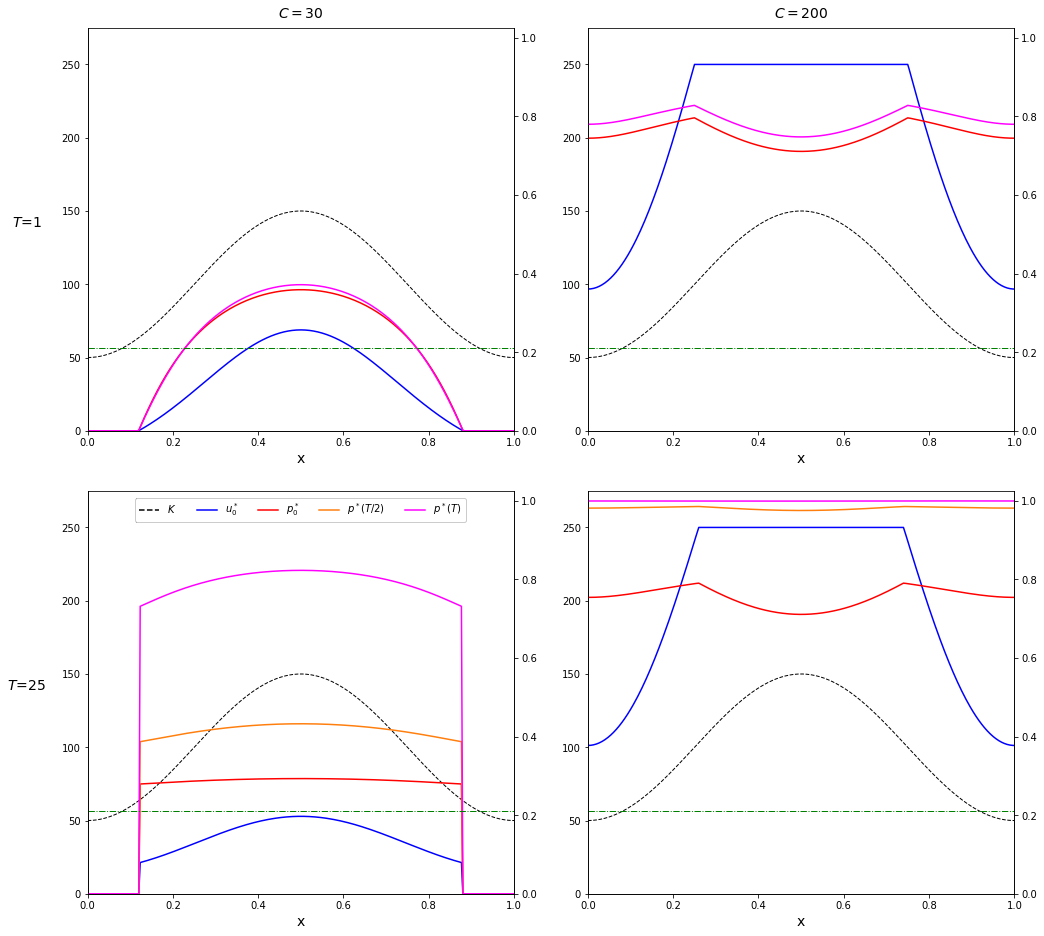
In Figure 3 we can see the results for . This choice models a scenario where mosquitoes are concentrated in the center of the domain studied and their concentration fades out as we move towards the boundaries. In the case (left column), we observe how the optimal strategy flattens and widens as increases. To understand this effect, we recall that in case , is decreasing with respect to . In other words, the Wolbachia-infected mosquitoes tend to be replaced by wild mosquitoes if they don’t surpass a critical threshold. Furthermore, if , is increasing with respect to , and therefore Wolbachia-infected mosquitoes take over the population without further intervention. For the parameters considered we have (The green dash-dotted line in Figure 3). According to our interpretation, since for small, is close to its initial condition, a value of below the threshold does not impact greatly the final result and reaching a bigger initial proportion in places where is higher is favoured. On the other hand, when is big, can be far from its initial condition. Hence, there is an incentive for to be above , since the proportion of Wolbachia-infected mosquitoes in the parts of the domain above will naturally increase with time. This also explains why the end of the release interval is abrupt. If the release is not going to achieve the critical proportion, it is better not to release. This effect can be seen clearly in the bottom-left graph and should be more pronounced the bigger is.
The changes between and in the case are imperceptible. A possible explanation is that in this case for all already in the first case. Therefore the proportion of Wolbachia-infected mosquitoes is going to increase with time everywhere. This case illustrates how is non-decreasing as increases, and how that is not necessarily the case of , which decreases when increases if . We recall that we have proven this monotonicity porperty for the case and in case but , which is the case in the bottom-right graph (, ). The only case where in Figure 3 is the one with , (bottom-left graph).
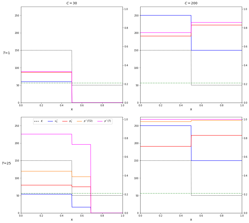
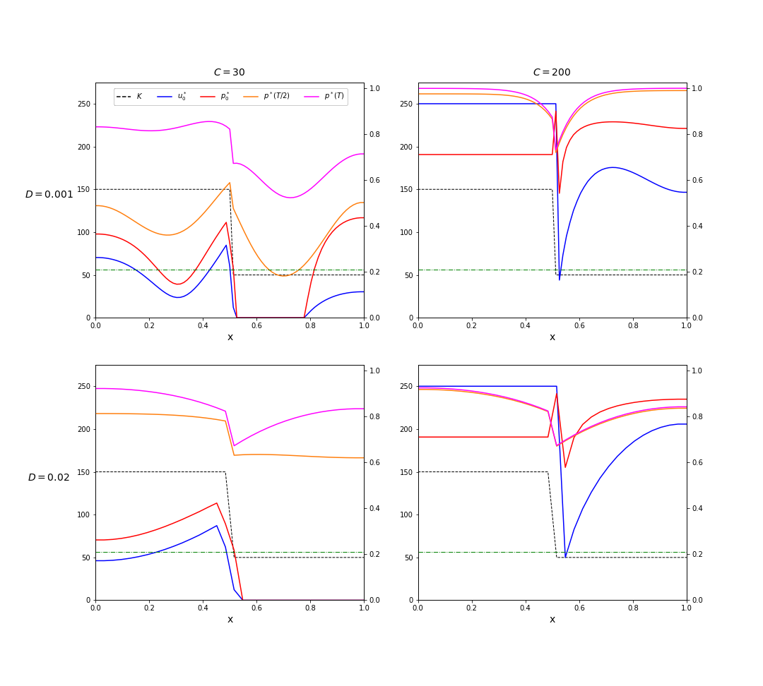
In Figure 4 we show the results for the simulations with . This figure represents a scenario with two patches of land with two very distinct conditions for mosquitoes, as it can be the case, for example, of an urban area close to a wetland. In the case we can observe again the difference between the short-term and long-term strategies. With reaching a higher proportion on the left patch is favoured, leaving the second patch untreated. Meanwhile, when the time horizon is increased, it also increases the incentive to release in a wider area above the critical proportion . Therefore the optimal releasing strategy consists in releasing a slightly smaller amount on the left patch in order to release in a certain domain in the right one.
In this case, on the bottom-left graph, we are in the case where , and thus the secondary problem must be solved for the values of in (see ()). Since is simple, the amount of mosquitoes released and the size of each subdomain of the right patch can be determined almost explicitely. For a fixed value of , the amount of mosquitoes released in the left patch is
analogously in the right patch wherever it is not . Therefore the size of the subdomain , where mosquitoes are released in the right patch is such that
This equality can be satisfied for different values of and . To find the optimal value and thus the optimal value of , we solve the one-dimensional optimization problem (), which in this case reads
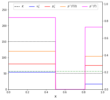
where and solve equation with initial condition and respectively. This solution, nonetheless, is what we have been calling unique ‘up to a rearrangement’. As long as the size of the domain where mosquitoes are released is preserved, the solution can be moved on the right half of the domain and still be optimal. In Figure 5 we show another choice for the solution.
Once again, in the case (right column) the solution does not change significantly when is increased. We can see how the monotonicity of with respect to is respected, but not for . In this case, releasing a smaller amount of mosquitoes in the right patch induces a higher initial proportion due to the smaller carrying capacity there.
4.2 The case with diffusion
So far, we have not considered diffusion in the system. Considering that mosquitoes do not disperse simplifies the analysis of the problem, but this comes at the expense of losing realism in the modeling. In this section we present some simulations in which diffusion is taken into account to see how the solutions presented above are modified. The simulations have been carried out using GEKKO (see [8]).
When diffusion is considered, as explained in the beginning of this paper, the equation governing the dynamics of the proportion is given by (2.7). Once again, we consider a single initial instantaneous release, which modifies equation (2.7) in an analogous way as the one explained for the non-diffusive case.
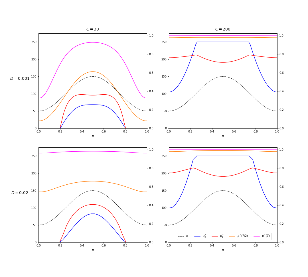
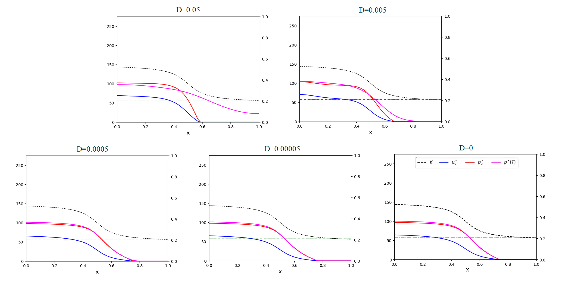
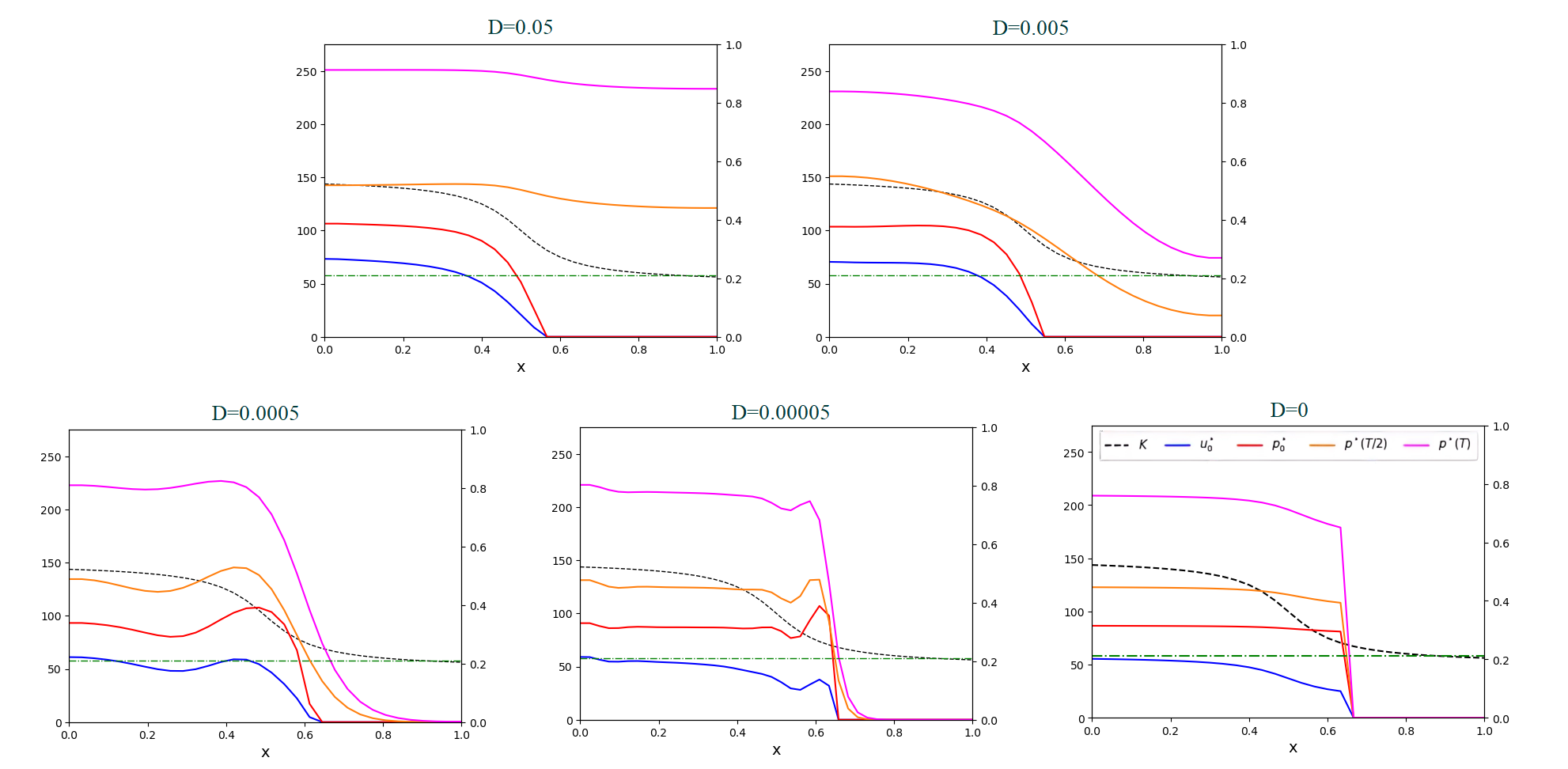
We are interested in observing how diffusion modifies the results presented so far. We place ourselves in the case with a bigger time horizon, , corresponding with the lower rows of Figures 3 and 4. We show the results for two different diffusion rate values: a smaller one, , and a bigger one, . In Figure 6, we set . In the left column, diffusion seems to concentrate the initial distribution of mosquitoes, making it slightly narrower and taller, although with a little decrease happening in the center of the release for a small diffusion value (upper left graph). Solutions in this case, nonetheless, seem quite robust to the addition of diffusion for the parameters considered. In the case of a piece-wise constant carrying capacity444Note that as defined is not differentiable and thus and are not defined. Nevertheless, we can always consider a differentialble function such that for , for and such that is smaller than the space step considered in the discretization done by the numerical algorithm implemented to compute the solutions. The carrying capacity in these simulations should be interpreted as the latter case. (Figure 7) the addition of diffusion immediately breaks the monotonicity of with respect to . This means that, contrary to the case without diffusion, releases do not need to be stronger where there are more wild mosquitoes, and that optimal releasing policies may be more complex. We also observe how mosquitoes are released in a way such that a big density difference is created in the area close to the boundary between patches. As we can see, specially in the bottom left graph, by setting an initial density difference in this boundary, an invasive wave propagates from the patch with a higher carrying capacity to the other one. It is also noteworthy that in this case a new stationary state appears strictly between and .
4.2.1 The limit case
We explore in this section the convergence when tends to zero of solutions for the problem where diffusion is considered, to the solutions of the non-diffusive case. This is a perspective section in the sense that no formal exploration of this convergence is done, but rather the exploration is carried numerically, leaving the formal analysis of the problem for future works.
More rigorously, let us consider , where solves
| (4.37) |
and where is a solution to the problem . Note that system (4.37) is the result of considering an impulsive release at initial time, , in equation (2.7), in case . Let us also consider, a solution to problem (), with being the initial condition of equation (2.13). The question we want to answer is: do we have convergence of the minimizers for the problem with diffusion to the minimizers of the problem without diffusion? Or more precisely, can we say that in some sense?
To explore this convergence we compare the results of the simulations obtained with our ad-hoc algorithm, developed exploiting theorems 3.6 and 3.8 (case ), with solutions obtained using GEKKO for the diffusive case with an ever decreasing . Let us consider the following carrying capacity: . This carrying capacity models an uneven distribution of mosquitoes, similar to the two-patch situation, but with a smooth transition between them. Again, .
We show the results for both cases, and . for the parameters of Table 1. In Figure 8 we show the results for . Both in case and , releases are stronger in the part of the domain where is higher, transitioning to zero in the part of the domain where is lower. Nonetheless, in case the tail of this transition is noticeably shorter than in the case. We observe how, as decreases, solutions transition from one configuration to the other, with a slight perturbation for . In case (Figure 9) the difference between and is much more notable. Indeed, the solution for is almost indistinguishible from the corresponding solution for , while in case the solution is flatter and wider, with a sharper edge (the reasons for this phenomenon have already been discussed in Section 4.1). Nevertheless, as decreases, we also observe how solutions are modified. At , the solution is remarkably similar to the case , perturbed only at the edge of the domain and in the transition to zero.
In conclusion, simulations suggest that, indeed, solutions converge in some sense when the diffusion rate tends to zero. That means that, despite the full problem being very hard to study, if the active motion of mosquitoes is sufficiently small which has been described to be the case in certain field releases (see, for instance, [16, 25]), the optimal distribution of a single release at initial time of Wolbachia-infected mosquitoes can be approximated by neglecting this motion completely without a big loss of precision. Therefore, beyond being a first step towards more sophisticate studies, our results may be meaningful under certain conditions despite the simplifications performed.
4.3 2D simulations
The method developed in this work can be applied in any dimension. Problems () and () can be solved using Theorems 3.6 and 3.8 or, at least, reduced to the one-dimensional optimization problem (), independently of the number of spatial dimensions considered. For a real application, nonetheless, the most interesting case is 2D.
Despite not presenting any novelties conceptually speaking, to illustrate the potential of the results, we show also two more simulations done in a 2D setting. We considerd the following carrying capacity
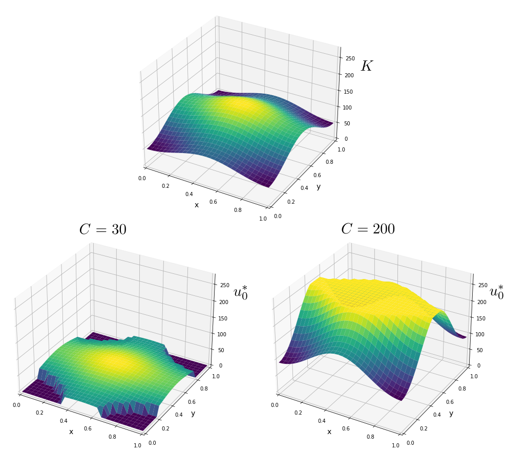
As in the case with , models a scenario with a higher concentration of mosquitoes towards the center of the domain and a smaller one towards the boundaries. Nevertheless, note that is not radially symmetric.
For the simulations we took , with . Once again, for the chosen parameters. The results of the simulations can be seen in Figure 10. We portray only the case for two values of . Results match the intuition one can have from the related 1D case . When a small amount of mosquitoes is considered, the solution is flat and wide to surpass the critical proportion in a bigger area, since the proportion of Wolbachia-infected mosquitoes will naturally increase in those places. Also, outside of this area for the reasons already exposed. On the other hand when a bigger amount of mosquitoes is considered, , the solution is bigger than everywhere and varies more rapidly, being higher where the carrying capacity is higher, but flattening out when is reached.
Acknowledgement
The authors would like to aknowledge warmly Pr. Yannick Privat for fruitful discussions and useful comments and remarks.
![[Uncaptioned image]](/html/2309.04192/assets/europe_flag.jpg) This project has received funding from the European Union’s Horizon 2020 research and innovation programme under the Marie Skłodowska-Curie grant agreement No 754362.
This project has received funding from the European Union’s Horizon 2020 research and innovation programme under the Marie Skłodowska-Curie grant agreement No 754362.
Appendix
Appendix A Numerical exploration of the parameter space for Hypothesis
Proposition A.1
Assuming and , then admits a single zero in .
Proof.
The existence of a zero of is straightforward to prove: we have , thus thanks to Rolle’s theorem, there exist two zeros of in . Then, applying again Rolle’s theorem, we prove the existence of some zero of , lying in between the two zeros of . Thus, in all generality.
Let us now prove the uniqueness of the zero of in . By computing the rational function , we see that where, denoting ,
Thus to conclude, it is enough to prove that has a unique zero in . Because holds, we find that
Then, using Descarte’s rule of signs, we find that has zero or two positive roots. However, since has at least one zero in , so does , so that admits exactly two positive roots. Meanwhile, applying the rule to implies that has one negative root.
Now, we set . In particular, the leading coefficient of is while one can prove that
Clearly has three real roots, and their product is given by . However, has at least one negative root since also does. Since the product of all three roots of is positive, has exactly two negative roots and one positive root. As a result, has exactly one root in , and the conclusion follows.
This section is devoted to a numerical exploration of the space of parameters, in order to establish the validity of Hypothesis (). For the exploration, we normalize the parameters assuming . The results are presented in Figures 11 and 12. To produce these images for a given pair of values , two random values for and are chosen, such that . If the randomly generated set of parameters are such that , the set is discarded. If indeed , then the Hypothesis () is tested. In blue, are the values of the parameters for which Hypothesis () is satisfied. In red, the values for which is not.
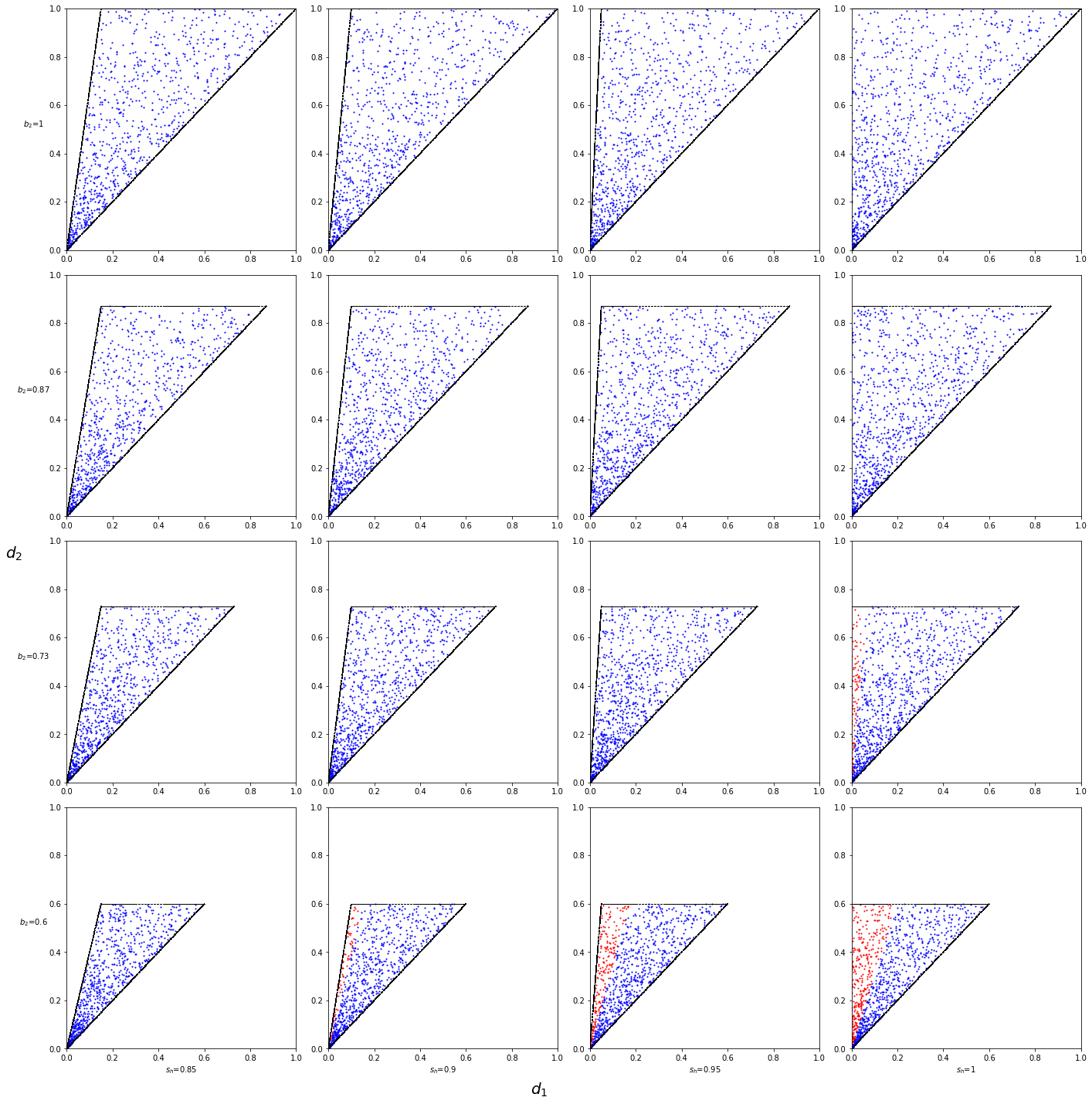
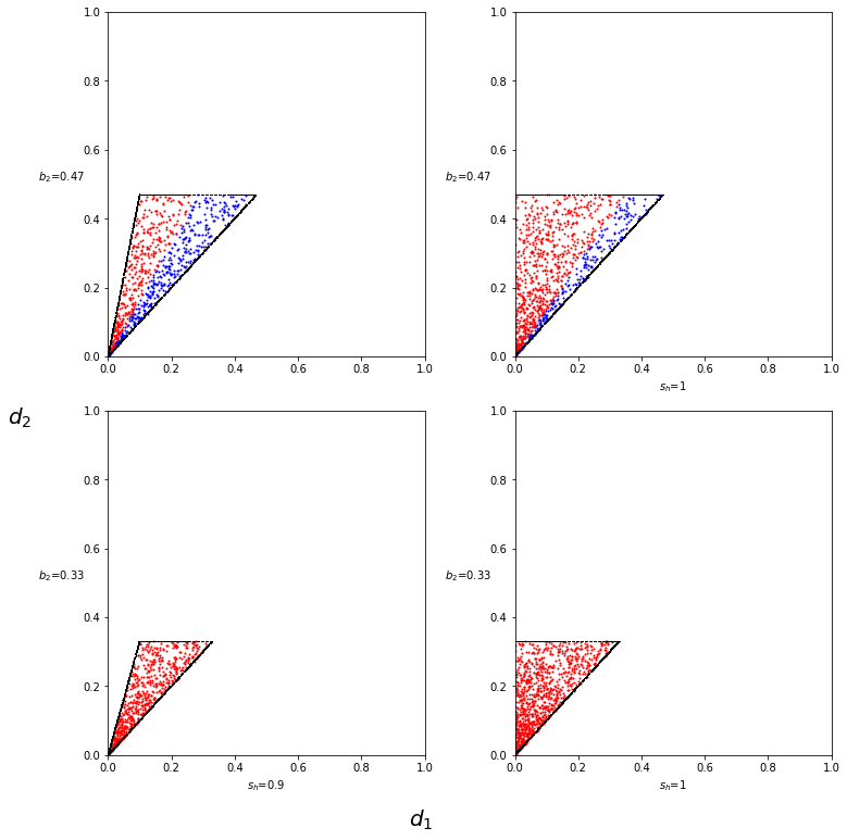
The condition can be written in terms of the other parameters,
Since and , this means that if , necessarily , thus these values can be excluded from the exploration. Indeed, the black lines wrapping the dots in Figures 11 and 12 are , and .
As we can see in Figure 11 and 12, Hypothesis is satisfied by most of the parameters of the parameter space. For high values of it is always satisfied (also for those values not shown in Figure 11). As decreases, red dots appear only when we have high values of and . Only for high values of and small values of the red dots dominate the picture. In a realistic scenario, based on the values for the parameters found in the literature [6, 13] we expect a high value of and and smaller values of and , for which hypothesis () is satisfied. The values of the parameters not satisfying Hypothesis () would represent a particular strain of Wolbachia that, in a certain variety of mosquito, would produce a high CI rate and a big penalty on their fertility, which, a priori, is not impossible.
Appendix B Comments on the existence of solutions for problem ()
In this work, we do not establish the existence of minimizers for problem () in all generality. Despite not exploring the matter separately, we do prove the existence of solutions in the case in Theorem 3.6. Indeed, in this theorem, we provide necessary conditions that solutions must satisfy. Then, in its proof, we exploit these conditions to narrow down the solution space, obtaining a single candidate to solution, . Since the constructed is the only candidate solution and we prove that , we conclude not only the existence but also the uniqueness of the solution (as already mentioned, up to a rearrangement in case is piecewise constant). Conversely, for the case , the candidate solution we construct in the proof of Theorem 3.8 by exploiting the necessary optimality conditions is not unique, but rather a whole family of candidates depending on a parameter . Hence we cannot conclude the existence of solutions from this result. On top, both theorems only hold under hypothesis ().
Although tackling comprehensively the existence of minimizers is beyond the scope of this work, we present here a partial result settling the existence in 1D, for all , for the case where is piecewise constant. This proof, nevertheless, cannot be easily extended to the general case.
Proposition B.1
Proof.
Let us write . We place ourselves in one of the intervals , where is constant.
Let us consider any function in this interval. We claim there exists a monotonic (decreasing or increasing) rearrangement of , that we will denote such that . To define this rearrangement, let us introduce, in a given interval ,
Then, we define in that interval as
The fact that such a rearrangement will respect is trivial since rearranging a function does not change its maximums or minimums (see [27]). Suppose , then
for every . is a continuous function, hence it is measurable. Therefore, since is non-negative and measurable we have
by equimeasurability of the rearrangement.
This implies that if , then . This reasoning can be easily extended to all of the subintervals. Therefore we have proved that is stable under rearrangements.
Let us define now
Observe that
with defined by (2.11). Indeed, if is minimizer of in , then
for every , where we are denoting by the solution to equation (2.13) with initial condition .
We can follow the same reasoning as before to prove that
for every . To see this clearly, we can write as a function of its initial condition by realising that can be written as
Defining as the antiderivative of vanishing at , , we can write
| (B.38) |
Both and its inverse are continuous functions and thus, so it is its composition. Therefore, is also a measurable function of and since it is non-negative both integrals are equal.
This implies that, if there exists a solution monotonic by intervals, there must also exist a solution in . Thus, we restrict our analysis to the first kind of functions.
Let us consider a minimizing sequence for problem (). We know it exists since is non-empty. Due to the fact that for all , a.e. in and using the monotonicity of on each interval , we deduce from Helly’s selection theorem (see [28]) that converges pointwisely to an element , up to a subsequence.
Basic properties of pointwise convergence lead us to conclude that a.e. in . Moreover, according to the Lebesgue dominated convergence theorem, one has
Indeed, we recall that is piecewise constant and thus it does not affect the convergence properties of the sequence under the integral. Therefore, . A similar reasoning shows that the sequence converges almost everywhere in and therefore, we have
according to (B.38). It follows that is indeed a solution to problem ().
References
- [1] K. Agbo Bidi, L. Almeida, and J.-M. Coron. Global stabilization of sterile insect technique model by feedback laws. working paper or preprint, July 2023.
- [2] L. Almeida, J. Bellver Arnau, and Y. Privat. Optimal control strategies for bistable ODE equations: application to mosquito population replacement. Appl. Math. Optim., 87(1):44, 2023. Id/No 10.
- [3] L. Almeida, J. Bellver Arnau, Y. Privat, and C. Rebelo. Vector-borne disease outbreak control via instant vector releases. working paper or preprint, Oct. 2022.
- [4] L. Almeida, M. Duprez, Y. Privat, and N. Vauchelet. Mosquito population control strategies for fighting against arboviruses. Mathematical Biosciences and Engineering, 16(6):6274, 2019.
- [5] L. Almeida, A. Haddon, C. Kermorvant, A. Léculier, Y. Privat, M. Strugarek, N. Vauchelet, and J. P. Zubelli. Optimal release of mosquitoes to control dengue transmission. In CEMRACS 2018—numerical and mathematical modeling for biological and medical applications: deterministic, probabilistic and statistical descriptions, volume 67 of ESAIM Proc. Surveys, pages 16–29. EDP Sci., Les Ulis, 2020.
- [6] L. Almeida, Y. Privat, M. Strugarek, and N. Vauchelet. Optimal releases for population replacement strategies: application to wolbachia. SIAM J. Math. Anal., 51(4):3170–3194, 2019.
- [7] T. Ant, C. Herd, V. Geoghegan, A. Hoffmann, and S. S.P. The wolbachia strain wau provides highly efficient virus transmission blocking in aedes aegypti. PLoS pathogens, 14(1):e1006815, January 2018.
- [8] L. Beal, D. Hill, R. Martin, and J. Hedengren. Gekko optimization suite. Processes, 6(8):106, 2018.
- [9] P.-A. Bliman. A feedback control perspective on biological control of dengue vectors by Wolbachia infection. European Journal of Control, 59:188–206, 2021.
- [10] K. Bourtzis. Wolbachia-based technologies for insect pest population control. In Transgenesis and the management of vector-borne disease, pages 104–113. Springer, 2008.
- [11] D. E. Campo-Duarte, O. Vasilieva, D. Cardona-Salgado, and M. Svinin. Optimal control approach for establishing wmelpop wolbachia infection among wild aedes aegypti populations. J. Math. Biol., 76(7):1907–1950, 2018.
- [12] A. Cristofaro and L. Rossi. Backstepping control for the sterile mosquitoes technique: stabilization of extinction equilibrium. working paper or preprint, 2023.
- [13] M. Duprez, R. Hélie, Y. Privat, and N. Vauchelet. Optimization of spatial control strategies for population replacement, application to wolbachia. ESAIM Control Optim. Calc. Var., 27:Paper No. 74, 30, 2021.
- [14] J. Z. Farkas and P. Hinow. Structured and unstructured continuous models for wolbachia infections. Bull. Math. Biol., 72(8):2067–2088, 2010.
- [15] A. Fenton, K. N. Johnson, J. C. Brownlie, and G. D. Hurst. Solving the wolbachia paradox: modeling the tripartite interaction between host, wolbachia, and a natural enemy. The American Naturalist, 178(3):333–342, 2011.
- [16] A. Hoffmann, B. Montgomery, J. Popovici, I. Iturbe-Ormaetxe, P. Johnson, F. Muzzi, M. Greenfield, M. Durkan, Y. Leong, Y. Dong, et al. Successful establishment of wolbachia in aedes populations to suppress dengue transmission. Nature, 476(7361):454, 2011.
- [17] H. Hughes and N. F. Britton. Modelling the use of wolbachia to control dengue fever transmission. Bull. Math. Biol., 75(5):796–818, 2013.
- [18] J. Kamtchum-Tatuene, B. L. Makepeace, L. Benjamin, M. Baylis, and T. Solomon. The potential role of wolbachia in controlling the transmission of emerging human arboviral infections. Current Opinion in Infectious Diseases, 30(1):108–116, February 2017.
- [19] Y. Li and X. Liu. A sex-structured model with birth pulse and release strategy for the spread of wolbachia in mosquito population. Journal of Theoretical Biology, 448:53–65, 2018.
- [20] E. H. Lieb and M. Loss. Analysis., volume 14 of Grad. Stud. Math. Providence, RI: American Mathematical Society (AMS), 2nd ed. edition, 2001.
- [21] I. Mazari, G. Nadin, and A. I. Toledo Marrero. Optimisation of the total population size with respect to the initial condition for semilinear parabolic equations: two-scale expansions and symmetrisations. Nonlinearity, 34(11):7510–7539, 2021.
- [22] G. Nadin, M. Strugarek, and N. Vauchelet. Hindrances to bistable front propagation: application to wolbachia invasion. J. Math. Biol., 76(6):1489–1533, 2018.
- [23] G. Nadin and A. I. Toledo Marrero. On the maximization problem for solutions of reaction-diffusion equations with respect to their initial data. Mathematical Modelling of Natural Phenomena, 15, 2020.
- [24] S. T. Ogunlade, M. T. Meehan, A. I. Adekunle, and E. S. McBryde. A systematic review of mathematical models of dengue transmission and vector control: 2010-2020. Viruses, 15(1), 2023.
- [25] S. L. O’Neill, P. A. f, A. P. Turley, G. Wilson, K. Retzki, I. Iturbe-Ormaetxe, Y. Dong, N. Kenny, C. J. Paton, S. A. Ritchie, J. Brown-Kenyon, D. Stanford, N. Wittmeier, N. P. Jewell, S. K. Tanamas, K. L. Anders, and C. P. Simmons. Scaled deployment of Wolbachia to protect the community from dengue and other Aedes transmitted arboviruses. Gates Open Res, 2:36, 2018.
- [26] Z. Qu, L. Xue, and J. M. Hyman. Modeling the transmission of wolbachia in mosquitoes for controlling mosquito-borne diseases. SIAM Journal on Applied Mathematics, 78(2):826–852, 2018.
- [27] J.-M. Rakotoson. Réarrangement relatif. Un instrument d’estimations dans les problèmes aux limites, volume 64 of Math. Appl. (Berl.). Berlin: Springer, 2008.
- [28] W. Rudin. Principles of mathematical analysis. International Series in Pure and Applied Mathematics. McGraw-Hill Book Co., New York-Auckland-Düsseldorf, third edition, 1976.
- [29] S. Sinkins. Wolbachia and cytoplasmic incompatibility in mosquitoes. Insect biochemistry and molecular biology, 34(7):723–729, 2004.
- [30] M. Strugarek and N. Vauchelet. Reduction to a single closed equation for 2-by-2 reaction-diffusion systems of lotka–volterra type. SIAM Journal on Applied Mathematics, 76(5):2060–2080, 2016.
- [31] E. Trélat. Contrôle Optimal: Théorie et Applications. Collection Mathématiques Concrètes. Vuibert, Paris, 2005.
- [32] D. Vicencio, O. Vasilieva, and P. Gajardo. Monotonicity properties arising in a simple model of Wolbachia invasion for wild mosquito populations. Mathematical Biosciences and Engineering, 20(1):1148–1175, 2023.
- [33] T. Walker, P. Johnson, L. Moreira, I. Iturbe-Ormaetxe, F. Frentiu, C. McMeniman, Y. Leong, Y. Dong, J. Axford, P. Kriesner, et al. The wmel wolbachia strain blocks dengue and invades caged aedes aegypti populations. Nature, 476(7361):450, 2011.