Gravitational waves from high-power twisted light

Abstract

Recent advances in high-energy and high-peak-power laser systems have opened up new possibilities for fundamental physics research. In this work, the potential of twisted light for the generation of gravitational waves in the high frequency regime is explored for the first time. Focusing on Bessel beams, novel analytic expressions and numerical computations for the generated metric perturbations and associated powers are presented. Compelling evidence is provided that the properties of the generated gravitational waves, such as frequency, polarisation states and direction of emission, are controllable by the laser pulse parameters and optical arrangements.

I Introduction

The importance of laboratory control of gravitational fields was first outlined by Weber [1] in 1960. Indeed, the successful generation and detection of terrestrially controlled gravitational waves (e.g. via mechanical or electromagnetic experimental schemes [1, 2, 3, 4, 5, 6, 7, 8, 9]) would undoubtedly usher in major advances in scientific research, in the same manner as the control of electromagnetic radiation. In addition, it is intriguing to note that, even though the action of gravity on light is well known and has been extensively studied over the past century, the converse - i.e. the way light acts as a source of gravity - remains, to a large extent, unexplored.

Of course, the idea of studying gravitational properties of electromagnetic fields is not an entirely new subject of investigation. Already in the early 1930’s, Tolman et al. [10] showed that parallel beams of light do not interact gravitationally, whereas anti-parallel beams do interact with twice the naive Newtonian force. Following that pioneering study, it has become clear that subtle effects are to be expected.

In 1962, as another example, Gertsenshtein posited that it was possible to convert electromagnetic and gravitational waves into each other via the wave resonance mechanism in a static magnetic field [11]. Then, just over a decade later, in 1975, Grishchuk and Sazhin proposed an elegant method to generate standing gravitational waves using excitations of an alternating electromagnetic field located inside a toroidal electromagnetic resonator [4].

Since the turn of the new millennium, there has been a large number of both high-energy and high-peak-power lasers being commissioned around the world [12]. Access to these facilities, along with advances in smaller-scale, ultra-short pulse laser systems, has enabled expertise in both the classical and quantum properties of light to increase dramatically. These extraordinary advances in both the quantum optics and high-energy density regimes make the current situation a conducive one in which to re-examine outstanding questions linking electromagnetic and gravitational concepts. High-energy lasers, in particular, provide an attractive platform to study gravitational aspects of light in laboratory settings, as the properties of the gravitational waves they generate are potentially controllable by specific optical arrangements and pulse properties.

The goal of this paper is to provide a new, first-principles calculation of gravitational waves associated with laser pulses that are generated by current and next generation high-energy laser facilities. Previous investigations have predominantly examined the gravitational effects of light modes characterized by radial extents negligible compared to their longitudinal dimensions, allowing them to be treated as ”needles of light” [13, 14, 15, 10] while completely ignoring the impact of any transverse structure. However, contemporary investigations has ventured into the realm of light modes with non-trivial transverse profiles. Particularly, research has been directed towards the gravitational properties of Gaussian and Bessel modes [16, 17]. However, these studies have remained focused on relatively-simple zeroth-order transverse modes. Thus, the examination of the full effects of transverse field structures, particularly phase structures, remains incomplete. As such, we have focused our attention on the higher-order Bessel modes endowed with orbital angular momentum (OAM) [18, 19] within the framework of gravitational wave emission. The effects of different optical parameters on the gravitational wave amplitudes as well as on the associated radiated power are presented. The angular distributions of these quantities around the source are also studied in detail.

Before delving more deeply into the calculations, it is emphasized here that the very concept of gravitational wave generation exhibits many non-intuitive effects as soon as one steps aside from usually considered astrophysical sources. Many subtle – and often implicit – hypotheses have to be made to unambiguously extract the wave part from the static part, keeping in mind that some steps remain somehow arbitrary [20]. Those conceptual issues will not be further discussed in this work but it is worth underlying that the whole reasoning raises complicated questions, in particular about energy which, in gravity, can only be defined in some specific regimes.

The article is organised as follows. In Section II, an introduction to the mathematical formulation for gravitational wave generation is provided. A discussion then follows, in Section III, on the properties of Bessel beams as a source of gravitational waves, broken down into different sub-sections highlighting: the proposed experimental set-up (A); the electromagnetic mode properties of Bessel beams (B); the spacetime deformations induced by Bessel pulses (C). There follows in Section IV further experimental considerations. In Section V, the results of numerical calculations are presented for current and future inertial confinement fusion facilities, including the limiting case of Bessel beams with no orbital angular momentum and finally specific cases where the Bessel beam does have orbital angular momentum. The implications of those results are then further discussed in Section VI. Section VII then summarises and concludes this paper.

II Formalism

The purpose of this section is to introduce readers unfamiliar with gravitational physics to the main concepts and equations that will be used to compute gravitational waves emitted by stress-energy distributions composed entirely of electromagnetic radiation.

The linearised Einstein field equations allow the description of weak gravitational fields in a perturbative approach and play a critical role in the study of gravitational waves [21, 22, 23].

The Einstein field equations without cosmological constant are given by:

$$R_{\mu\nu}-\frac{1}{2}g_{\mu\nu}R=-\kappa T_{\mu\nu}\leavevmode\nobreak\ ,$$ (1)

$g_{\mu\nu}$ being the metric tensor, $T_{\mu\nu}$ the stress-energy tensor and $R_{\mu\nu}$ and $R$ being respectively the Ricci tensor and scalar, that can be written in terms of second derivatives of $g_{\mu\nu}$. As usual $\left\{\mu,\nu\right\}$ indices range from $0$ to $3$. The smallness (compared to unity) of the prefactor $\kappa=8\pi Gc^{-4}\sim 10^{-43}$ underlines how difficult it is to significantly bend spacetime.

Considering small perturbations around the flat spacetime metric one writes:

$$g_{\mu\nu}=\eta_{\mu\nu}+h_{\mu\nu}\leavevmode\nobreak\ ,\leavevmode\nobreak\ \leavevmode\nobreak\ |h_{\mu\nu}|\ll 1\leavevmode\nobreak\ ,$$ (2)

with $\eta_{\mu\nu}=\text{diag}(1,-1,-1,-1)$.

The linearised Ricci tensor is thus given by:

$$R_{\mu\nu}=\frac{1}{2}\left(\partial_{\mu}\partial_{\nu}h+\Box h_{\mu\nu}-\partial_{\mu}\partial_{\rho}h^{\rho}_{\nu}-\partial_{\nu}\partial_{\rho}h^{\rho}_{\mu}\right)+\mathcal{O}\left(h^{2}\right),$$ (3)

Where $\Box\equiv\partial_{\mu}\partial^{\mu}=c^{-2}\partial^{2}/\partial t^{2}-\nabla^{2}$ denotes the d’Alembertian operator. The linearised Ricci scalar is further obtained by contraction of the previous tensor:

$$R=\Box h-\partial_{\rho}\partial_{\mu}h^{\mu\rho}+\mathcal{O}\left(h^{2}\right)\leavevmode\nobreak\ .$$ (4)

One useful quantity for simplifying the writing of the linearised Einstein field equations is the trace-reversed metric perturbation $\bar{h}_{\mu\nu}$:

$$\bar{h}_{\mu\nu}\equiv h_{\mu\nu}-\frac{1}{2}\eta_{\mu\nu}h^{\alpha}_{\alpha}\leavevmode\nobreak\ .$$ (5)

Substituting equations (3), (4) and (5) into equation (1) leads to the following linearisation of Einstein’s set of equations:

$$\Box\bar{h}_{\mu\nu}+\eta_{\mu\nu}\partial_{\sigma}\partial_{\rho}\bar{h}^{\sigma\rho}-\partial_{\nu}\partial_{\rho}\bar{h}^{\rho}_{\mu}-\partial_{\mu}\partial_{\rho}\bar{h}^{\rho}_{\nu}=-2\kappa T_{\mu\nu}\leavevmode\nobreak\ .$$ (6)

Further simplifications can be performed by invoking the Lorenz (or harmonic) gauge:

$$\partial_{\mu}\bar{h}^{\mu\nu}=0\leavevmode\nobreak\ ,$$ (7)

Under which previous equations simplify considerably. They reduce to:

$$\Box\bar{h}_{\mu\nu}=-2\kappa T_{\mu\nu}\leavevmode\nobreak\ .$$ (8)

In block matrix form, the electromagnetic stress energy tensor is given by:

$$T^{\mu\nu}=\begin{pmatrix}u&\vline&\vec{N}/c\\ \hline\cr\vec{N}/c\ &\vline&-\sigma_{i,j}\end{pmatrix}\leavevmode\nobreak\ ,$$ (9)

With $u$, $\vec{N}$ and $\sigma_{ij}$ being respectively the electromagnetic field energy density, the associated Poynting vector and the rank 2 Maxwell tensor, whose expressions are given by:

$$u = \frac{\epsilon_{0}c}{2}(E^{2}+c^{2}B^{2})\leavevmode\nobreak\ ,$$ (10)

$$\vec{N} = \frac{\vec{E}\times\vec{B}}{\mu_{0}}\leavevmode\nobreak\ ,$$ (11)

$$\sigma_{ij} = \epsilon_{0}c(E_{i}E_{j}+c^{2}B_{i}B_{j})-u\delta_{i,j}\leavevmode\nobreak\ .$$ (12)

Taking care to consider sources of finite dimensions, use is made of the standard Green’s function approach to find solutions to the linearised field equations (8) under the form:

$$\bar{h}^{\mu\nu}\left(t,\vec{x}\right)=\frac{4G}{c^{4}}\int_{\mathcal{V}}\frac{T^{\mu\nu}\left(t-\frac{|\vec{x}-\vec{x^{\prime}}|}{c},\vec{x^{\prime}}\right)}{|\vec{x}-\vec{x^{\prime}}|}d^{3}x^{\prime}\leavevmode\nobreak\ ,$$ (13)

Where $\mathcal{V}$ corresponds to the volume of the source, $\vec{x^{\prime}}$ denotes the spatial coordinates of any source point and $|\vec{x}-\vec{x^{\prime}}|$ therefore corresponds to the distance between a certain point of the source and the location at which the field $\bar{h}_{\mu\nu}$ is evaluated.

One assumes the compact source approximation, i.e. at a distance $r$ from a source of characteristic length $L$ such that $r\gg L$. Introducing $\vec{x}\equiv r\hat{n}$ one can therefore approximate $|\vec{x}-\vec{x^{\prime}}|=r-\vec{x^{\prime}}\cdot\hat{n}+\mathcal{O}((\frac{L}{r})^{2})$, leading to:

$$\bar{h}^{\mu\nu}\left(t,\vec{x}\right)=\frac{1}{r}\frac{4G}{c^{4}}\int_{\mathcal{V}}T^{\mu\nu}\left(t-\frac{r}{c}+\frac{\vec{x^{\prime}}\cdot\hat{n}}{c},\vec{x^{\prime}}\right)d^{3}x^{\prime}\leavevmode\nobreak\ ,$$ (14)

At first order in $L/r$. In equation (14), $\hat{n}$ is a unit vector connecting the center of the source to any coordinate point in the far-field.

The reader’s attention is drawn to a very well-known problem: the symmetric metric perturbation $h_{\mu\nu}$ contains 10 degrees of freedom which, in the treatment provided here, have been reduced to 6 using the Lorenz gauge condition $\partial_{\mu}\bar{h}^{\mu\nu}=0$.

The residual gauge freedoms have caused a lot of confusion in the early days of the field. In a 1922 paper [24], A.S. Eddington stated that “Weyl has classified plane gravitational waves into three types: (1) longitudinal-longitudinal modes, (2) longitudinal-transverse modes, and (3) transverse-transverse modes.” Those modes correspond to the six remaining degrees of freedom of the metric perturbation in the Lorenz gauge.

It was shown that only the transverse-transverse modes are radiative [24, 25]. In general the pure gauge modes are not associated with a spacetime curvature and thus cannot be measured by any apparatus. A general treatment of the classification of metric perturbations was later conducted by Liftshitz in 1946 [26], while more modern treatments of this topic can be found in [25, 27]. The physical components of a metric perturbation are extracted by transforming the perturbation into the so-called transverse-traceless (TT) gauge [28].

To do so, one can use the lambda projector tensor [28, 23]:

$$\Lambda(\hat{n})_{ij,kl} = P_{ik}P_{jl}-P_{ij}P_{kl}\leavevmode\nobreak\ ,$$ (15)

$$P_{ij} = \delta_{ij}-n_{i}n_{j}\leavevmode\nobreak\ ,$$ (16)

With indices $\left\{i,j\right\}$ running from 1 to 3, such that:

$$\bar{h}_{ij}^{TT}=\Lambda(\hat{n})_{ij,kl}\bar{h}^{kl}\leavevmode\nobreak\ .$$ (17)

It should be emphasised here that solutions to the linearised Einstein field equations presented in (13) or (14), give the form of the trace-reversed metric $\bar{h}_{\mu\nu}$ which differs a priori from the spacetime deformation $h_{\mu\nu}$ that one was initially interested in. However if $h^{\mu}_{\mu}=0$, as in the TT gauge, then $\bar{h}^{\mu\nu}=h^{\mu\nu}$. The quantities $\bar{h}_{\mu\nu}^{TT}$ and $h_{\mu\nu}^{TT}$ are therefore equal.

The writing of perturbations in the $TT$ gauge is highly advantageous as it allows for the retention of solely the physical degrees of freedom, i.e. the two allowable polarisation states. In this gauge the linearised Riemann curvature tensor $R_{\mu\nu\alpha\beta}$ is linked to $h_{\mu\nu}^{TT}$ such that

$$R_{i0j0}=-\frac{1}{2}\frac{\partial^{2}{h}_{ij}^{TT}}{\partial t^{2}}\leavevmode\nobreak\ .$$ (18)

In vacuum, all other non-zero components of the Riemann tensor can be deduced from $R_{i0j0}$ by the mean of its symmetries and Bianchi identities. Moreover, in the linearised theory, the linearised Riemann tensor is invariant under residual gauge (i.e. coordinate) transformations.

As presented in [28, 23], a gravitational wave stress-energy tensor is defined from the Riemann tensor at quadratic order in $h$, leading to the following expression for the power per unit solid angle:

$$\frac{dP}{d\Omega}=\frac{r^{2}c^{3}}{32\pi G}\left<\frac{\partial h_{ij}^{TT}}{\partial t}\frac{\partial h^{ij,TT}}{\partial t}\right>,$$ (19)

Where the average is performed over many reduced wavelengths $\lambdabar\sim h/\partial h$ and $r$ denotes the radial distance to the source. This quantity corresponds to the radiation flux measurable by an observer located along any radial direction with respect to the center of the source.

III Bessel pulses as sources of gravitational waves

Now that the general formalism has been established, it is now possible to consider the generation of gravitational waves from so-called twisted light. This is a type of laser mode which has attracted considerable interest over the past couple of decades due to its ability to carry orbital angular momentum (OAM) in addition to the well known spin angular momentum caused by their polarisation [29]. The two most well studied twisted light modes are the Laguerre-Gaussian [30, 31] and Bessel modes [32, 33, 34]. They are characterised by an azimuthal phase-dependence in the transverse profile of their field, $E(x^{\mu})\propto e^{il\phi}$, where $l\in\mathbb{Z}$ is the topological index which quantises the OAM state. This can be seen by calculating the total angular momentum of the electromagnetic fields of these modes, defined as:

$$\vec{J} = \iint\vec{\mathcal{J}}dS\leavevmode\nobreak\ ,$$ (20)

$$\vec{\mathcal{J}} = \vec{r}\crossproduct(\vec{E}\crossproduct\vec{B})\leavevmode\nobreak\ ;$$ (21)

where $\vec{J}$ is the total angular momentum of the electromagnetic field and $\vec{\mathcal{J}}$ is its angular momentum density [35]. The latter can be rigorously derived by the standard method of applying Noether’s theorem to the electromagnetic Lagrangian density and considering the conserved quantities due to its rotational invariance. It can then be readily shown that, for example, the time-averaged total angular momentum of a Laguerre-Gaussian mode is [36]:

$$\langle\vec{J}\rangle\propto(l+\sigma)\hat{z}\leavevmode\nobreak\ ;$$ (22)

where $\hat{z}$ is the unit vector of the direction of propagation of the mode, $l$ is the aforementioned azimuthal topological index, quantifying the contribution to the angular momentum from its orbital component, and $\sigma=\left\{0,\pm 1\right\}$ characterises the spin component and depends on the polarisation of the mode, be it linear, left- or right-circular. It should be noted that, unlike the convention in atomic physics, $l$ does not denote the total OAM but represents its projection along the propagation direction of the laser.

Since they were first characterised, twisted light modes have found applications in various fields spanning from non-linear vacuum and high-power laser-plasma interactions [37, 38, 39, 40, 41] to quantum and classical communication technologies [42, 43, 44]. Consequently, scientists have devoted efforts to push the development of techniques enabling their generation and control [45, 46, 47]. Our motivation for analysing the spacetime perturbations caused by these modes is that this additional OAM may be used to generate gravitational waves and control their characteristics.

Although most investigations of the effects of orbital angular momentum consider Laguerre-Gaussian modes, the latter are less suitable for our purposes as they have a short length over which their peak intensity is constant, similarly to any other Gaussian mode. As such, our focus will be directed towards exploring Bessel modes as a source of gravitational waves.

III.1 Bessel modes

The interest in Bessel modes as solutions to the electromagnetic wave equation started mainly due to one specific feature that attracted a lot of attention, their ”non-diffractive” propagation [32]. In essence, unlike Gaussian modes whose transverse spatial profile changes as they propagate, Bessel modes maintain a constant spatial profile, thereby maintaining a constant peak intensity. Additionally, they are ”self-healing”, their transverse spatial profile will re-establish itself after any partial obstruction. These incredible properties have made them very attractive for a variety of use cases in optics and laser-matter interactions.

The original formulation of Bessel modes relied on solving the scalar version of the electromagnetic wave equation in cylindrical coordinates [32]. However, one can achieve exact vector solutions that have the same properties by considering a particular linear superposition of plane wave solutions. Specifically, the infinite superposition of plane waves whose wave-vectors lie tangent to surface of a cone of half-angle $\alpha$, and are arranged around the circular base of that cone:

$$\vec{E}{(x^{\mu},\phi)}=i^{l}E_{0}e^{i(k_{\mu}(\phi)x^{\mu}+l\phi)}\hat{n}(\phi)\leavevmode\nobreak\ ;$$ (23)

where $l$ the azimuthal mode number whose significance will become apparent later on, $k^{\mu}(\phi)=(\omega/c,\vec{k}(\phi))$ and $x^{\mu}=(ct,\vec{x})$ denote the wave and position four-vectors respectively, and $\phi=\arctan(y/x)$ is the azimuthal position, in cylindrical coordinates, of the wave-vector on the conical surface. The spatial components of the wave four-vector are given by:

$$\vec{k}(\phi) = -k_{0}\sin(\alpha)\hat{\rho}+k_{0}\cos(\alpha)\hat{z}\leavevmode\nobreak\ ,$$ (24)

$$\hat{n}(\phi) = -\hat{\phi}\leavevmode\nobreak\ ;$$ (25)

where $\hat{\rho}=\cos(\phi)\hat{x}+\sin(\phi)\hat{y}$ and $\hat{\phi}=-\sin(\phi)\hat{x}+\cos(\phi)\hat{y}$ are the standard cylindrical unit vectors. It can be easily checked that the spatial components of $k^{\mu}(\phi)$ always satisfy the transverse propagation condition $\hat{n}(\phi)\cdot\vec{k}(\phi)=0$. The electric field of a vector Bessel beam can thus be written as [37]:

$$\vec{E}(\vec{x},t)=\frac{1}{2\pi}\int_{0}^{2\pi}\vec{E}{(x^{\mu},\phi)}d\phi\leavevmode\nobreak\ .$$ (26)

The corresponding magnetic field is computed from the Maxwell-Faraday equation ($\nabla\times\vec{E}=-\partial\vec{B}/\partial t$) [35]. The components of both fields are:

$$E_{x} = \frac{E_{0}}{2}\left[J_{l+1}(\beta\rho)\sin(\omega t-k_{z}z+(l+1)\phi)-J_{l-1}(\beta\rho)\sin\left(\omega t-k_{z}z+(l-1)\phi\right)\right]\leavevmode\nobreak\ ,$$ (27)

$$E_{y} = -\frac{E_{0}}{2}\left[J_{l+1}(\beta\rho)\cos(\omega t-k_{z}z+(l+1)\phi)+J_{l-1}(\beta\rho)\cos\left(\omega t-k_{z}z+(l-1)\phi\right)\right]\leavevmode\nobreak\ ,$$ (28)

$$E_{z} = 0\leavevmode\nobreak\ ,$$ (29)

$$B_{x} = \cos(\alpha)\frac{E_{0}}{2}\left[J_{l+1}(\beta\rho)\cos(\omega t-k_{z}z+(l+1)\phi)+J_{l-1}(\beta\rho)\cos(\omega t-k_{z}z+(l-1)\phi)\right]\leavevmode\nobreak\ ,$$ (30)

$$B_{y} = \cos(\alpha)\frac{E_{0}}{2}\left[J_{l+1}(\beta\rho)\sin(\omega t-k_{z}z+(l+1)\phi)-J_{l-1}(\beta\rho)\sin(\omega t-k_{z}z+(l-1)\phi)\right]\leavevmode\nobreak\ ,$$ (31)

$$B_{z} = \sin(\alpha)\frac{E_{0}}{c}J_{l}(\beta\rho)\cos(\omega t-k_{z}z+l\phi)\leavevmode\nobreak\ ,$$ (32)

where $\rho=\sqrt{x^{2}+y^{2}}$ denote the radial distance in cylindrical coordinates, $k_{z}=k_{0}\cos(\alpha)$ is the propagation constant, and $\beta=k_{0}\sin(\alpha)$ is the transverse wave-vector which characterises the beam’s ”waist”. The latter two satisfy the dispersion relation $\omega^{2}=c^{2}(\beta^{2}+k_{z}^{2}+l^{2}/\rho^{2})$. The functions of the form $J_{n}(\tau),n\in\mathbb{Z}$ are the n-th order Bessel functions of the first kind.

From the mathematical expression of the spatial distribution of the fields, it is clear that the transverse profile of the Bessel modes is invariant along their propagation direction since the transverse wave vector $\beta$ is completely independent from the longitudinal $z$-coordinate.

One calculates the angular momentum density of these fields using equation (21), for which the explicit expression of the angular momentum density is given by:

$$<\vec{\mathcal{J}}>=\frac{\epsilon_{0}E_{0}}{c}\left[\frac{l}{k_{0}}J_{l}^{2}(\beta\rho)\hat{z}-\frac{lz\sin(\alpha)}{\beta\rho}J_{l}^{2}(\beta\rho)\hat{\rho}\right.$$

$$-\left.\rho\cos(\alpha)\frac{J_{l+1}^{2}(\beta\rho)-J_{l-1}^{2}(\beta\rho)}{2}\hat{\phi}\right].$$ (33)

By integrating formula (33) over the transverse profile of the mode, the radial and azimuthal components integrate to 0 and the total angular momentum is thus quantised by the azimuthal mode number $l$ and lies along the propagation direction $\hat{z}$. As in the case of the Laguerre-Gaussian modes, this observation shows that the electromagnetic field distribution’s orbital angular momentum (OAM) is indeed described by the topological index $l$.

III.2 Proposed experimental setup

Ideal Bessel beams with infinite extent are obviously non-physical as they carry infinite energy. Realistic Bessel beams can however be generated over a finite region of space by a variety of methods, see e.g. [45, 46]. In practice in the context of high-power laser systems, it is important to consider the laser-induced damage threshold of transmission optics. Transmissive optics under the passage of a high-power laser pulse are prone to optical damage. In order to overcome the limitations associated with optical damage in transmission optics, the generation of Bessel beams can be effectively achieved by employing reflective axicon optics [45, 48, 49], for which optical damage can be mitigated with the use of suitably sized laser beams. Reflective axicons, by crossing the wavefront of the incident Gaussian laser pulse over a conical volume, produce an interference pattern that results in a Bessel mode over a conical region of space. Such a setup is depicted in figure 1, for which the curve inside the conical region of created by the crossed wave fronts is a graphical illustration of the emergent Bessel mode. In this figure $z$, $\rho$ and $\phi$ are the usual cylindrical co-ordinates.

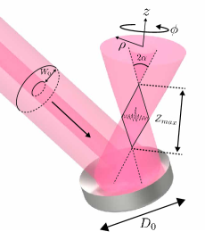
Figure 1: Schematic example of Bessel pulse generation. $D_{0}$ is the diameter of the axicon optic, $W_{0}$ characterises the incident beam diameter, $Z_{max}$ denotes the depth of focus and $\alpha$ the half-cone angle.

The depth of focus (DOF) $Z_{max}$ is defined as the region of space over which the beam waist is assumed to remain constant. It can be expressed as:

$$Z_{max}=\frac{W_{0}}{2\sin(\alpha)}\leavevmode\nobreak\ ;$$ (34)

where $W_{0}$ is the incident beam diameter (that can reach 1 meter [12]) that is constrained by $W_{0}\leq D_{0}$ and $\alpha$ is the half cone angle appearing in figure 1. Unlike their Laguerre-Gaussian counterparts whose energy distributions are localised to the central lobe, Bessel modes are able to propagate without diffraction due to their delocalised energy distribution [50]. Bessel modes depth of field can therefore exceed the Rayleigh range of a Laguerre-Gaussian mode [32, 33, 51, 30, 31].

The radial extent of this cylinder is normally not constant along the entire propagation path. However, to facilitate the computation of the characteristics of the emitted gravitational wave radiation, it is assumed that the Bessel mode is confined within a cylindrical subset of the conical volume over which the Bessel mode is normally defined. An explicit depiction of the cylindrical approximation of the source volume $\mathcal{V}$ generated by a Gaussian laser pulse on a reflective axicon whose inner surface is inclined at an angle $\gamma$ is given in figure 2.

$$\mathcal{V}\coloneqq(\rho,\phi,z)\in[0,D/2]\times[0,2\pi]\times[-L/2,L/2]$$ (35)

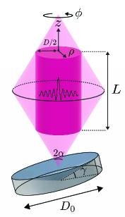
Figure 2: Cylindrical integration region.

The axicon base angle $\gamma$ has been incorporated into figure 2, as it is occasionally mentioned in the literature [45, 52]. It is related to the half-cone angle by $\alpha=2\gamma$, however in the context of this article it will not be used. The interaction length $L$ is bounded such that $L\leq Z_{\text{max}}$. As an example, for $W_{0}=1$ and $\alpha=0.6$, the corresponding $Z_{\text{max}}$ is around $1.77$ms, for which the interaction length $L$ must satisfy $L\leq 1.77$m. The cylinder diameter can then be deduced geometrically from $L$ and $\alpha$ to be $D=(Z_{max}-L)\tan(\alpha)$. Importantly, the confinement of the Bessel mode within the cylindrical region introduces an additional constraint, namely $Z_{max}<c\tau_{p}$, $\tau_{p}$ being the temporal width of the pulse.

The presence of the constraint on $Z_{max}$ allows for the existence of a period of time during which the conical region containing the Bessel mode can be completely filled. This simplification greatly reduces the computational complexity since the motion of the pulse envelope no longer needs to be considered. Within this particular setup, the duration of the gravitational wave signal $\tau_{s}$ can be approximated by the time duration over which the laser pulse completely fills the conical region of space generated by the crossed wave fronts of the reflective axicon, such that:

$$\tau_{s}\approx\tau_{p}-\frac{L}{c}\leavevmode\nobreak\ .$$ (36)

It is important to acknowledge that Bessel modes are not limited to propagating along null paths in spacetime, as they can exhibit both subluminal and superluminal speeds. It should be noted that the super-luminal speeds of the Bessel mode do not violate causality, but are instead a consequence of the contact point of the crossing wave fronts created by the axicon optic having an effective velocity that can exceeds the speed of light. This is analogous to the ”scissor paradox”. This characteristic allows these modes to radiate throughout their entire propagation path [13]. For the considered setup, effects on the generated gravitational wave signal due to the motion of the temporal envelope of a Bessel mode, such as the Doppler effect, can not be investigated. Nonetheless, the outcomes of this work are expected to hold true when considering velocities well below the speed of light. Specifically, because the strain of gravitational waves is dependant on the energy contained within the source, we expect that the estimated strain amplitude of a gravitational wave generated by a laser pulse whose energy is independant of its frequency to be independent of the velocity of the pulse envelope.
The effect of the pulse envelope velocity of a Bessel mode with arbitrary velocity is of theoretical interest and remains to be addressed in future research endeavors.

III.3 Analytical calculation of spacetime deformations induced by Bessel pulses

III.3.1 The stress-energy tensor

To compute the expected spacetime deformations one first fixes a frame and computes the expression of $T^{\mu\nu}$ in this frame. One chooses the frame in which the expressions of the Bessel modes’ $\vec{E}$ and $\vec{B}$ fields given in equations (27 - 32) are expressed, i.e. the frame represented in figure 2, whose origin is located at center of the domain $z\in[-L/2,L/2]$ over which the electromagnetic field distribution is defined. The $z$-axis is aligned with the Gaussian pulse direction of propagation anterior to the reflective axicon, and the $x$ and $y$ -axes point respectively vertically and towards the reader. This frame is denoted as the ”laboratory frame (LF)”. In the following, the physical quantities are expressed by default in this frame, unless stated otherwise. This convention will be of particular importance when computing the induced spacetime deformations, as the form of $h_{\mu\nu}$ depends explicitly on the chosen frame.

Plugging equations (27 - 32) into the form of the stress-energy tensor presented in equation (9) permits the computation of $T_{\mu\nu}$. To do so the following functions are introduced:

$$\xi_{0} \equiv J_{l}(\beta\rho)\cos\left[\omega t-k_{z}z+l\phi\right]\leavevmode\nobreak\ ,$$ (37)

$$\xi_{+} \equiv J_{l+1}(\beta\rho)\cos\left[\omega t-k_{z}z+(l+1)\phi\right]$$

$$+J_{l-1}(\beta\rho)cos\left[\omega t-k_{z}z+(l-1)\phi\right]\leavevmode\nobreak\ ,$$

$$\xi_{-} \equiv J_{l+1}(\beta\rho)\sin\left[\omega t-k_{z}z+(l+1)\phi\right]$$

$$-J_{l-1}(\beta\rho)\sin\left[\omega t-k_{z}z+(l-1)\phi\right]\leavevmode\nobreak\ ,$$

Such that the energy density takes the form

$$T_{00}=\frac{\epsilon_{0}c}{2}E_{0}^{2}\left[\left(1+\cos(\alpha)^{2}\right)\left(\xi_{+}^{2}+\xi_{-}^{2}\right)+\sin(\alpha)^{2}\xi_{0}^{2}\right]\leavevmode\nobreak\ .$$ (40)

Due to Bessel functions properties, an increase of the orbital angular momentum parameter $l$ leads to a decrease of the energy density of the individual lobes of $T_{00}$. This does not mean that the total energy is decreased. Indeed the number of the ”lobes” increases with $l$, such that the total energy is conserved.

The previous energy density can be written as the sum of a static and an oscillating component. The static one reads:

$$T_{00}^{\text{Stat}}=\frac{\epsilon_{0}c}{2}E_{0}^{2}\left[\left(1+\cos(\alpha)^{2}\right)\left(J_{l-1}(\beta\rho)^{2}\right.\right.$$

$$\left.\left.+J_{l+1}(\beta\rho)^{2}\right)+\frac{1}{2}\sin(\alpha)^{2}J_{l}(\beta\rho)^{2}\right]\leavevmode\nobreak\ .$$ (41)

Once integrated over the source volume, it corresponds to an effective mass on the order of $m_{\text{eff}}\sim\mathcal{E}/c^{2}\simeq 10^{-11}$ kg for a 1 MJ laser, $\mathcal{E}$ being the energy of the laser pulse. This is a tiny value, several orders of magnitude below the Planck mass. This is the reason why the chances to detect a gravitational effect due to light directly as a Newtonian force or as tidal effect seem extremely low, which motivates the focus on gravitational waves.

The oscillating component of the electromagnetic field energy density is given by:

$$T_{00}^{\text{Osc}}=\frac{\epsilon_{0}c}{2}E_{0}^{2}\left[\left(1+\cos(\alpha)^{2}\right)J_{l+1}(\beta\rho)J_{l-1}(\beta\rho)\right.$$

$$+\left.\frac{1}{4}\sin^{2}(\alpha)J_{l}(\beta\rho)^{2}\right]\cos\left[2\omega t-2k_{z}z+2l\phi\right]\leavevmode\nobreak\ .$$ (42)

The $T_{0i}$ components are not of any significance for this study since, as enhanced by equation (17), they do not contribute to the form of $\bar{h}_{\mu\nu}^{TT}$ expressed in the traceless-transverse gauge. Even so, the expression of the Poynting vector is provided for the interested reader:

$$T_{0j}=\epsilon_{0}cE_{0}^{2}\cos(\alpha)\begin{pmatrix}\xi_{+}\xi_{0}\\ \xi_{-}\xi_{0}\\ \xi_{+}^{2}+\xi_{-}^{2}\end{pmatrix}\leavevmode\nobreak\ .$$ (43)

The $T_{ij}$ components are given by the Maxwell tensor ones $\sigma_{ij}$, that can be expressed as:

$$T_{ij}=\sigma_{ij}\equiv\sigma_{ij}^{D}+\sigma_{ij}^{ZZ}+\sigma_{ij}^{+}+\sigma_{ij}^{\times}+\sigma_{ij}^{XZ}+\sigma_{ij}^{YZ},$$ (44)

with

$$\sigma_{ij}^{D} = \frac{\epsilon_{0}cE_{0}^{2}}{2}\sin^{2}(\alpha)\begin{pmatrix}-\xi_{0}^{2}&0&0\\ 0&-\xi_{0}^{2}&0\\ 0&0&\xi_{0}^{2}\end{pmatrix},$$ (45)

$$\sigma_{ij}^{ZZ} = -\frac{\epsilon_{0}cE_{0}^{2}}{2}[1+\cos^{2}(\alpha)]\begin{pmatrix}0&0&0\\ 0&0&0\\ 0&0&\xi_{+}^{2}+\xi_{-}^{2}\end{pmatrix},$$ (46)

$$\sigma^{+}_{ij} = \frac{\epsilon_{0}cE_{0}^{2}}{2}\sin^{2}(\alpha)\begin{pmatrix}\xi_{+}^{2}-\xi_{-}^{2}&0&0\\ 0&-\xi_{+}^{2}+\xi_{-}^{2}&0\\ 0&0&0\end{pmatrix},$$ (47)

$$\sigma^{\times}_{ij} = \epsilon_{0}cE_{0}^{2}\sin^{2}(\alpha)\begin{pmatrix}0&\xi_{+}\xi_{-}&0\\ \xi_{+}\xi_{-}&0&0\\ 0&0&0\end{pmatrix},$$ (48)

$$\sigma_{ij}^{XZ} = \frac{\epsilon_{0}cE_{0}^{2}}{2}\sin^{2}(\alpha)\begin{pmatrix}0&0&\xi_{0}\xi_{+}\\ 0&0&0\\ \xi_{0}\xi_{+}&0&0\end{pmatrix},$$ (49)

$$\sigma_{ij}^{YZ} = \frac{\epsilon_{0}cE_{0}^{2}}{2}\sin^{2}(\alpha)\begin{pmatrix}0&0&0\\ 0&0&\xi_{0}\xi_{-}\\ 0&\xi_{0}\xi_{-}&0\end{pmatrix}.$$ (50)

The Maxwell tensor has been subdivided into three groups:

• $\left\{\sigma_{ij}^{D},\sigma_{ij}^{ZZ}\right\}$, which coefficients depend on $l$;

• $\left\{\sigma_{ij}^{+},\sigma_{ij}^{\times}\right\}$, which coefficients depend on $l\pm 1$;

• $\left\{\sigma_{ij}^{XZ},\sigma_{ij}^{YZ}\right\}$, which coefficients depend on $2l\pm 1$.

In the following analysis, it will become evident that it is possible to treat these sets of source terms independently.

From these expressions it can be ensured that $\partial_{\mu}T^{\mu\nu}=0$, thus that the solution equation (13) satisfies the harmonic gauge condition [28].

III.3.2 Spacetime deformations

Considering the symmetries of the system, one writes $\hat{n}\equiv(\sin(\theta),0,\cos(\theta))$. The variable $\theta$ introduced here denotes the angle in the $z-x$ plane between the optical axis $z$ and the propagation direction of the emitted gravitational waves.

Solutions to the Einstein field equations in the far-field region are obtained following equation (14) and performing the integration in cylindrical coordinates over the cylindrical source volume $\mathcal{V}$ depicted in figure 2. Unlike, e.g. the seminal paper [10], this analysis does not focus on the total gravitational action of the laser pulse, but only on the associated waves. Any static component can therefore be safely ignored.

In the following, subsequent definitions will be used:

$$\bar{h}_{0}(r) \equiv \frac{4\pi\epsilon_{0}cE_{0}^{2}GL}{\beta^{2}c^{5}r}\leavevmode\nobreak\ ,$$ (51)

$$\psi_{q}(t,r) \equiv 2\omega(t-r/c)+2q(\phi-\pi/2)\leavevmode\nobreak\ ,$$ (52)

$$\Gamma_{q}(\theta) \equiv \int_{0}^{\frac{D\beta}{2}}\tau J_{q}^{2}(\tau)J_{2q}\left(\frac{\omega\tau}{c\beta}\sin(\theta)\right)d\tau\leavevmode\nobreak\ ,$$ (53)

$$\Lambda^{\pm}_{s}(\theta) \equiv \int_{0}^{\frac{D\beta}{2}}\tau J_{l}(\tau)J_{l\pm 1}(\tau)J_{s}\left(\frac{\omega\tau}{c\beta}\sin(\theta)\right)d\tau$$ (54)

$$\eta(\theta) \equiv \frac{\omega L}{c}\left[\cos(\theta)-\cos(\alpha)\right]\leavevmode\nobreak\ ,$$ (55)

With $q\in\{l,Q\}$, where $Q\in\{2,l\pm 1\}$, and $s\in\{1,2l\pm 1\}$. The $\Gamma_{q}(\theta)$ and $\Lambda^{\pm}_{s}(\theta)$ represent the radial integrals of the Green’s function solutions in the far-field over a planar circular aperture of diameter $D$, for which the substitution $\tau\equiv\beta\rho$ has been used.

For clarity, only the dependencies upon the coordinates $\left\{t,r,\theta\right\}$ are written down explicitly, and not those related to optical parameters such as $\beta$, $\omega$, etc.

Previous definitions then allow one to introduce the terms:

$$\bar{h}_{D} \equiv \frac{1}{2}\bar{h}_{0}(r)\sin^{2}(\alpha)\Gamma_{l}(\theta)\text{Sinc}\left[\eta(\theta)\right]\sin(\psi_{q})\leavevmode\nobreak\ ,$$ (56)

$$\bar{h}_{ZZ} \equiv 2\bar{h}_{0}(r)\left[1+\cos^{2}(\alpha)\right]\Gamma_{l}(\theta)\text{Sinc}\left[\eta(\theta)\right]$$ (57)

$$\times\cos(\psi_{q})\leavevmode\nobreak\ ,$$

$$\bar{h}_{+}^{(Q)} \equiv \bar{h}_{0}(r)\sin^{2}(\alpha)\Gamma_{Q}(\theta)\text{Sinc}\left[\eta(\theta)\right]\cos(\psi_{q})\leavevmode\nobreak\ ,$$ (58)

$$\bar{h}_{\times}^{(Q)} \equiv \bar{h}_{0}(r)\sin^{2}(\alpha)\Gamma_{Q}(\theta)\text{Sinc}\left[\eta(\theta)\right]\sin(\psi_{q})\leavevmode\nobreak\ ,$$ (59)

$$\bar{h}_{XZ}^{\pm,(s)} \equiv \frac{1}{4}\bar{h}_{0}(r)\sin(2\alpha)\Lambda^{\pm}_{s}(\theta)\text{Sinc}\left[\eta(\theta)\right]\cos(\psi_{q})\leavevmode\nobreak\ ,$$ (60)

$$\bar{h}_{YZ}^{\pm,(s)} \equiv \frac{1}{4}\bar{h}_{0}(r)\sin(2\alpha)\Lambda^{\pm}_{s}(\theta)\text{Sinc}\left[\eta(\theta)\right]\sin(\psi_{q})\leavevmode\nobreak\ ,$$ (61)

$$\bar{h}_{N} \equiv 2\bar{h}_{0}(r)\cos(\alpha)\Gamma_{l}(\theta)\text{Sinc}\left[\eta(\theta)\right]\cos(\psi_{q})\leavevmode\nobreak\ .$$ (62)

Introducing the following expressions:

$$\bar{h}_{+} \equiv 2\bar{h}_{+}^{(2)}+\bar{h}_{+}^{(l+1)}+\bar{h}_{+}^{(l-1)}\leavevmode\nobreak\ ,$$ (63)

$$\bar{h}_{\times} \equiv 2\bar{h}_{\times}^{(2)}+\bar{h}_{\times}^{(l+1)}+\bar{h}_{\times}^{(l-1)}\leavevmode\nobreak\ ,$$ (64)

$$\bar{h}_{XZ} \equiv \bar{h}_{XZ}^{+,(1)}+\bar{h}_{XZ}^{-,(1)}+\bar{h}_{XZ}^{+,(2l+1)}+\bar{h}_{XZ}^{-,(2l-1)}\leavevmode\nobreak\ ,$$ (65)

$$\bar{h}_{YZ} \equiv \bar{h}_{YZ}^{+,(1)}-\bar{h}_{YZ}^{-,(1)}+\bar{h}_{YZ}^{+,(2l+1)}-\bar{h}_{YZ}^{-,(2l-1)}\leavevmode\nobreak\ ,$$ (66)

the $\mu\nu$ components of the oscillating metric perturbation in the laboratory frame finally read:

$$\small\bar{h}_{\mu\nu}=\begin{pmatrix}\bar{h}_{D}-\bar{h}_{ZZ}&\bar{h}_{XZ}&\bar{h}_{YZ}&\bar{h}_{N}\\ \bar{h}_{XZ}&\bar{h}_{+}-\bar{h}_{D}&\bar{h}_{\times}&\bar{h}_{XZ}\\ \bar{h}_{YZ}&\bar{h}_{\times}&-\bar{h}_{+}-\bar{h}_{D}&\bar{h}_{YZ}\\ \bar{h}_{N}&\bar{h}_{XZ}&\bar{h}_{YZ}&\bar{h}_{ZZ}+\bar{h}_{D}\end{pmatrix}\leavevmode\nobreak\ .$$ (67)

The expressions (63 - 66) and in turn equation (67) can be simplified after a deeper analysis of the $\Gamma_{q}(\theta)$ and $\Lambda^{\pm}_{s}(\theta)$ functions. For this purpose the parameter $\zeta_{D}$ is introduced:

$$\zeta_{D}\equiv\frac{\omega D}{c}\leavevmode\nobreak\ .$$ (68)

This parameter corresponds to the maximal value of the argument of the second Bessel function appearing in equation 53, since $\tau/\beta=\rho\leq D$. It depends on the frequency of the laser pulse $\omega$ as well as on the diameter of the source cylindrical volume $D$. Typical values of $D$ range from 1 m [12] to the diffraction limit (corresponding to half a wavelength), typically of the order of $10^{-7}$m [51]. Considering $w\simeq 10^{15}$ Hz, the associated values of $\zeta_{D}$ therefore range from unity up to $10^{7}$.

Figure 3 shows, for different values of the index $q$, the maximal values of $\Gamma_{q}(\theta)$ obtained spanning $\theta\in\left[0;2\pi\right]$. Whatever the value of $\zeta_{D}$, the dominant function is always the one with $q=0$. Thus, in the subsequent analysis, only cases where $q=0$ are considered as they correspond to the main sources of gravitational waves.

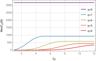
Figure 3: Dependencies of $\text{Max}\left[\Gamma_{q}(\theta)\right]$ upon the $\zeta_{D}$ parameter obtained varying the angle $\theta\in\left[0;2\pi\right]$. The values $L=1$ mm and $D=1$ mm have been chosen for clarity.

Since $q\in\left\{2,l,l\pm 1\right\}$, the study is restricted to values of the topological index such that $l\in\left\{0,\pm 1\right\}$. Higher values of $l$ lead to Bessel functions of smaller amplitudes and therefore to $\Gamma_{q}(\theta)$ also being smaller. As a consequence, dominant contributions to the $\bar{h}_{+}$ and $\bar{h}_{\times}$ functions presented in equations (63) and (64) will come from $\bar{h}_{+}^{(0)}$ and $\bar{h}_{\times}^{(0)}$ terms and all the other $\bar{h}_{+}^{(n)}$ and $\bar{h}_{\times}^{(n)}$, $n\neq 0$, can be disregarded.

Similar deductions can be made about the $\Lambda^{\pm}_{s}(\theta)$ functions. Since $l\in\mathbb{Z}$ it follows that $s$ is a non-zero integer, whatever the value of $l$. Subsequently there will never be a $s=0$ component in $\bar{h}_{XZ}$ and $\bar{h}_{YZ}$ and they can always be neglected compared to $\left\{\bar{h}_{D},\bar{h}_{ZZ},\bar{h}_{+},\bar{h}_{\times}\right\}$.

After simplifications, spacetime perturbations take the new form:

$$\small\bar{h}_{\mu\nu}\simeq\begin{pmatrix}\bar{h}_{D}-\bar{h}_{ZZ}&0&0&\bar{h}_{N}\\ 0&\bar{h}_{+}-\bar{h}_{D}&\bar{h}_{\times}&0\\ 0&\bar{h}_{\times}&-\bar{h}_{+}-\bar{h}_{D}&0\\ \bar{h}_{N}&0&0&\bar{h}_{ZZ}+\bar{h}_{D}\end{pmatrix}\leavevmode\nobreak\ ,$$ (69)

in which the functions $\bar{h}_{+}$ and $\bar{h}_{\times}$ have also been simplified such that:

$$\bar{h}_{+} \simeq \bar{h}_{+}^{(l+1)}+\bar{h}_{+}^{(l-1)}\leavevmode\nobreak\ ,$$ (70)

$$\bar{h}_{\times} \simeq \bar{h}_{\times}^{(l+1)}+\bar{h}_{\times}^{(l-1)}\leavevmode\nobreak\ .$$ (71)

It is now possible to extract the radiative, or physical, components by projecting $\bar{h}_{ij}$ into the TT gauge associated with any observer in the $\hat{n}$ direction around the source. This projection involves only the spatial components $\bar{h}_{ij}$ of the $\bar{h}_{\mu\nu}$ given equation (69). The temporal-temporal $00$ and crossed $0i$ or $i0$ components never contribute to the expressions of the perturbations in the TT gauge and, from now on, the $\bar{h}_{N}$ function will no longer play any role.

As previously stated, due to the symmetries of the system this study is restricted to the $z-x$ plane, the $z$-axis corresponding to the direction along which the pulse propagates, such that $\hat{n}=(\sin(\theta),0,\cos(\theta))$. Using the Lambda projector and following (17), the total metric perturbation in the TT gauge is written as the sum of four contributions:

$$\bar{h}_{\mu\nu}^{TT}=\bar{h}_{\mu\nu}^{D,TT}+\bar{h}_{\mu\nu}^{ZZ,TT}+\bar{h}_{\mu\nu}^{+,TT}+\bar{h}_{\mu\nu}^{\times,TT}\leavevmode\nobreak\ .$$ (72)

The respective terms entering formula (72) are given by:

$$\bar{h}_{\mu\nu}^{D,TT}=\left(\begin{array}[]{cccc}0&0&0&0\\ 0&\cos^{2}(\theta)\left[1-\cos(2\theta)\right]&0&\cos(\theta)\sin(\theta)\left[\cos(2\theta)-1\right]\\ 0&0&\cos(2\theta)-1&0\\ 0&\cos(\theta)\sin(\theta)\left[\cos(2\theta)-1\right]&0&\sin^{2}(\theta)\left[1-cos(2\theta)\right]\\ \end{array}\right)\bar{h}_{D}\leavevmode\nobreak\ ,$$ (73)

$$\bar{h}_{\mu\nu}^{ZZ,TT}=\left(\begin{array}[]{cccc}0&0&0&0\\ 0&\cos^{2}(\theta)\left[1-\cos(2\theta)\right]&0&\cos(\theta)\sin(\theta)\left[\cos(2\theta)-1\right]\\ 0&0&\cos(2\theta)-1&0\\ 0&\cos(\theta)\sin(\theta)\left[\cos(2\theta)-1\right]&0&\sin^{2}(\theta)\left[1-cos(2\theta)\right]\\ \end{array}\right)\bar{h}_{ZZ}\leavevmode\nobreak\ ,$$ (74)

$$\bar{h}_{\mu\nu}^{+,TT}=\left(\begin{array}[]{cccc}0&0&0&0\\ 0&\frac{1}{2}\cos^{2}(\theta)\left[\cos^{2}(\theta)+1\right]&0&-\frac{1}{2}\sin(\theta)\cos(\theta)\left[\cos^{2}(\theta)+1\right]\\ 0&0&-\frac{1}{2}\left[1+\cos^{2}(\theta)\right]&0\\ 0&-\frac{1}{2}\sin(\theta)\cos(\theta)\left[\cos^{2}(\theta)+1\right]&0&\frac{1}{2}\sin^{2}(\theta)\left[\cos^{2}(\theta)+1\right]\\ \end{array}\right)\bar{h}_{+}\leavevmode\nobreak\ ,$$ (75)

$$\bar{h}_{\mu\nu}^{\times,TT}=\left(\begin{array}[]{cccc}0&0&0&0\\ 0&0&\cos^{2}(\theta)&0\\ 0&\cos^{2}(\theta)&0&-\sin(\theta)\cos(\theta)\\ 0&0&-\sin(\theta)\cos(\theta)&0\\ \end{array}\right)\bar{h}_{\times}\leavevmode\nobreak\ .$$ (76)

By straightforward inspection it can be verified that $n^{i}\bar{H}_{ij}=0$ where $\bar{H}_{ij}\in\{\bar{h}_{ij}^{D,TT},\bar{h}_{ij}^{zz,TT},\bar{h}_{ij}^{+,TT},\bar{h}_{ij}^{\times,TT}\}$. The far-field metric perturbations in the TT gauge are indeed transverse to the propagation direction of the gravitational waves for all values of $\theta$.

The detailed study of those perturbations will be performed in the following sections, for different values of the orbital angular momentum parameter $l$.

It might seem surprising to the reader that the matrices in equations (73) and (74) take the same form, as $\bar{h}_{D}$ and $\bar{h}_{ZZ}$ contribute in different ways to $\bar{h}_{\mu\nu}$ in (67).

However, it has been previously demonstrated that the $\sigma_{ij}^{D}$ term in the Maxwell tensor gives rise to metric perturbations in which spatial components exhibit the following form:

$$\bar{h}_{ij}^{D}=a(t,\vec{x})\begin{pmatrix}1&0&0\\ 0&1&0\\ 0&0&0\end{pmatrix}+b(t,\vec{x})\begin{pmatrix}0&0&0\\ 0&0&0\\ 0&0&1\end{pmatrix}\leavevmode\nobreak\ ,$$ (77)

the functions $a(t,\vec{x})$ and $b(t,\vec{x})$ depending on spatial and temporal coordinates $x^{\mu}=(ct,\vec{x})$. The first term exhibits a form similar to polarization modes known as ”breathing” modes, which can be present in alternative theories of gravity in which additional polarisation states of gravitational waves exist, such as Brans-Dicke or Horndeski theories [53, 54]. However, in standard General Relativity, such modes are not present. Therefore, when considering the projection in the TT gauge of both terms entering equation (77), only the second one matters, and this term is of the same form as the metric perturbation generated by the purely longitudinal source term $\sigma_{ij}^{ZZ}$.

IV Further Experimental Considerations

IV.0.1 Considered laser facilities

In order to discuss the generation of gravitational waves by current day laser facilities or those expected to become operational in the coming decades, we introduce two types of laser systems [12]:

• The Laser MegaJoule (LMJ) [55, 56] and National Ignition Facility (NIF) [57] which are both currently operational and situated in France and in the United States of America, respectively.

• The NIF Advanced Radiography Capability (ARC) facility [58] and the Station of Extreme Light (SEL) [59] in Shanghai. The former is operational and the latter is expected to be commissioned later this decade.

The mega-joule class facilities, designed for inertial confinement fusion (ICF) and nuclear stockpile stewardship research, both allocate a portion of their shot time to the academic community for Discovery Science applications [55, 56]. The NIF and LMJ deliver multiple kilo-joule class beams, with the NIF having 192 beams and LMJ having 240 beams. Recent advancements in plasma optics and beam-combiners suggest that both LMJ and NIF may soon be capable of generating a single beamline with an energy up to 0.8 MJ in a single 20 ns pulse at 351 nm [60].

The NIF ARC facility was developed to enhance the capabilities of high brightness X-ray probes for studying high energy density conditions. NIF ARC employs four of NIF’s 351 nm laser beams (one quad), with each beam split into two halves. This configuration enables the generation of eight peta-Watt class beams, delivering energy ranging from 0.4 kJ to 1.7 kJ, with pulse lengths ranging from 1.3 to 38 ps. Each beam reaches a maximum peak power of 0.5 PW. Consequently, the total energy delivered to the target within 38 ps is 13.6 kJ (358 TW).

The Station of Extreme Light (SEL), is also a kiloJoule class laser facility, dedicated to high-intensity laser-matter interaction research. Its primary objective is to generate the most intense laser pulses ever achieved on Earth. Specifically, the SEL aims to produce a pulse with a power of 100 PW resulting from a 1.5 kJ, 15 fs pulse [59].

The standard electromagnetic mode of laser pulses at any of those facilities, like in any laser facility, is not a Bessel mode. The generation of such modes requires appropriate optics. Notably, Bessel modes can be generated by directing a single beam onto an axicon optic. Even if not all laser systems consist of a single beam, recent advancements in plasma optics and beam-combiners suggest that it may soon be feasible for both LMJ and NIF to produce a single beam-line with an energy capacity of up to 0.8 MJ in a 20 ns pulse at a wavelength of 351 nm [60]. This super beam could then be utilised to generate a Bessel mode pulse by employing axicon optics.

IV.0.2 Power normalisation

In order to perform numerical simulations, the Bessel modes power must first be normalised. Since ideal Bessel beams partition their energy equally among the lobes of the beam radial profile, setting the power $P_{0}=\epsilon_{0}E_{0}^{2}\beta^{-2}$ adds spurious energy to the system when a Bessel mode beam waist $\beta^{-1}$ is decreased at constant $D$. This is compensated for by equating the power of the incident beam on the axicon optic to the power of the generated Bessel mode, fixing the energy content by conservation of energy [50], such that:

$$\mathcal{N}_{B}^{-1}P_{0}=\frac{\epsilon_{0}cE_{0}^{2}}{2\beta^{2}}\leavevmode\nobreak\ ,$$ (78)

Where the normalisation factor $\mathcal{N}_{B}$ is defined as:

$$\mathcal{N}_{B}=\cos(\alpha)\int_{0}^{\frac{D\beta}{2}}\tau\left[J_{l-1}^{2}(\tau)+J_{l+1}^{2}(\tau)\right]d\tau\leavevmode\nobreak\ .$$ (79)

IV.0.3 Axicon optic

The functions $\bar{h}_{D}$, $\bar{h}_{ZZ}$, $\bar{h}_{+}^{Q}$ and $\bar{h}_{\crossproduct}^{Q}$ presented in equations (56 - 59) give the amplitudes of the generated gravitational waves. Their maximal values, corresponding to the highest gravitational wave signal, depend, among other parameters, on the half cone angle $\alpha$.

One considers a focused Bessel mode associated with large values of $\alpha$ so that all previous but $\bar{h}_{ZZ}$ functions are maximized. It is important to note that increasing the half cone angle cannot result in arbitrarily small beam waists. This limitation stems from the diffraction-limited nature of Bessel modes. The diffraction limited spot size $W_{D}$ is given in terms of the numerical aperture $N_{a}$ by [51, 61]:

$$W_{D}=\frac{\lambda}{2\pi N_{a}}\leavevmode\nobreak\ .$$ (80)

Equating the beam width $\beta$ to the reciprocal of the diffraction limit beam waist $W_{D}^{-1}$ leads to $N_{a}=\sin(\alpha)$. Axicon optics have demonstrated the ability to reach numerical apertures of 0.75 [45]. Therefore the maximum achievable half cone angle is:

$$\alpha_{\text{max}}=0.848\simeq\frac{\pi}{3.7}\leavevmode\nobreak\ \text{rads}\leavevmode\nobreak\ .$$ (81)

V Numerical simulations

This section is kept brief and numerical results of the amplitude and angular distribution of the Bessel mode generated gravitational wave are presented, for the case of the topological index being zero and unity with minimal comments. Further discussions are provided in section VI.

V.1 Bessel pulses with no orbital angular momentum: the $l=0$ case

At first sight one is tempted to claim that, without orbital angular momentum carried by the laser pulse, no gravitational waves are expected to be produced by the system. Neglecting phase noise effects this statement appears to be erroneous because, in addition to the twisting due to the orbital angular momentum, an additional effect is in play.

It is true that when $l=0$, $\xi_{+}^{2}-\xi_{-}^{2}=\xi_{+}\xi_{-}=0$ and the $\sigma_{ij}^{+}$ equation (47) and $\sigma_{ij}^{\crossproduct}$ equation (48) contributions to the Maxwell tensor both vanish. As a consequence $\bar{h}_{+}$ and $\bar{h}_{\times}$ also completely vanish. In addition, it has been demonstrated that the spacetime deformations generated by the $\sigma_{ij}^{XZ}$ and $\sigma_{ij}^{YZ}$ components given in (49) and (50), i.e $\bar{h}_{XZ}$ and $\bar{h}_{YZ}$, can be neglected. Nevertheless, the $\bar{h}_{D}$ and $\bar{h}_{ZZ}$ deformations, generated by $\sigma_{ij}^{D}$ from (45) and $\sigma_{ij}^{ZZ}$ from (46), remain.

This poses the question: if the pulse carries no orbital angular momentum, what is the source of the gravitational waves? To match with intuition, one can rely on $\sigma_{ij}^{D}$ and $\sigma_{ij}^{ZZ}$ both being diagonal. Since the trace of the stress-energy tensor must vanish, i.e $T_{\mu}^{\mu}=0$, the sum of their coefficients are related to the expression of the energy density $T_{00}$ given in equation (40). As enhanced by the formula (42), this energy exhibits oscillations which, once integrated over the cylindrical source volume, remain present. This oscillating electromagnetic energy content induces oscillating pressure along the $x$, $y$ and $z$ axes, leading to radiative oscillations of spacetime.

In the absence of orbital angular momentum, radiative metric perturbations are therefore still expected and their form in the $\hat{n}$ oriented TT gauges are given by:

$$\bar{h}_{\mu\nu,l=0}^{TT}\simeq\bar{h}_{\mu\nu}^{D,TT}+\bar{h}_{\mu\nu}^{ZZ,TT}\leavevmode\nobreak\ .$$ (82)

Of course, it is possible that accumulated phase errors, e.g. those associated with propagation of the laser light in the amplifier media, might negate this effect. However, the low B-integrals normally associated with peta-Watt class laser systems suggest that this is unlikely to manifest itself. Similarly, numerical studies of phase errors of amplified seed beams in Raman amplifiers also indicate that these are also unlikely to play a significant role in pulses associated with beam-combiners [62, 63].

V.1.1 Frequencies ($l=0$)

The generated gravitational wave frequency is obviously a key parameter, especially regarding detection aspects.

The time dependence of the linearised Einstein field equation solutions $\bar{h}_{\mu\nu}^{D,TT}$ and $\bar{h}_{\mu\nu}^{ZZ,TT}$ presented in (73) and (74) is located in $\bar{h}_{D}$ and $\bar{h}_{ZZ}$. Those functions both oscillate in time with a phase given by $\psi_{q}(t,r)$, defined in equation (52). Gravitational waves generated by oscillations of the electromagnetic energy content therefore oscillate at twice the laser frequency. This result was indeed already obvious from the expression of the energy density shown in (40). For a NIF’s 351 nm laser pulse [60] this corresponds to

$$\omega_{g}^{l=0}=2\omega\simeq 8.55\times 10^{14}\leavevmode\nobreak\ \text{Hz}\leavevmode\nobreak\ .$$ (83)

V.1.2 Amplitudes ($l=0$)

As the coefficients of the matrices equations (73) and (74) involve only trigonometric functions that will mainly impact the angular distributions of the waves and not their maximal amplitude, the latter property is estimated by the sum of the $\bar{h}_{D}$ and $\bar{h}_{ZZ}$ functions established in (56) and (57) respectively.

The maximal value of this sum is represented in figure 4 for parameters (energy and pulse width) given by the four laser facilities presented section IV: the SEL 1.5 kJ, the NIF-QUAD 20 kJ, the NIF/LMJ 0.8 MJ and the NextICF 5MJ [12, 55, 56, 57, 58, 59].

The switching to dashed lines corresponds to distances to the source under which the assumed far-field approximation is not valid anymore. So why show the gravitational wave amplitudes below the domain of validity of our computations? The answer is because one interesting aspect of laser generated gravitational waves is the proximity to the source at which a detector can be located, in order to exploit the $1/r$ dependence of the gravitational waves amplitude. It might be that, in the future, one can try to detect gravitational perturbations with detection systems placed at very short distances, using e.g. other laser systems such as presented in [64].

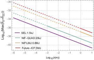
Figure 4: Maximum gravitational wave amplitude as a function of the radial distance to the source $r$. The plot includes data from four laser facilities, including a potential next-generation (5 MJ, 250 TW) high-gain ICF laser facility called ”Future-ICF”. The values of the optical parameters used are $l=0$, $L=\tau_{p}/2$ and $D=10\mu m$, where ”$\tau_{p}$” is obtained from [12, 59]. Dashed lines are used when the radial distance ”r” falls below the range where the far-field approximation holds.

V.1.3 Angular distributions ($l=0$)

Now consider the angular distribution of the previous metric deformations. In order to better visualise the dependencies to the optical parameters, we consider the laser frequency to be variable and $L$ fixed at $L=1$mm instead of $L=c\tau_{p}/2$ unless stated otherwise.

As long as $\zeta_{D}<1$, $\Gamma_{0}(\theta)$ is maximised in all directions and therefore independent of $\theta$, see Appendix A for more details. The whole angular dependence is in this case due to the $\text{Sinc}\left[\eta(\theta)\right]$ function. To better characterise its effect we introduce:

$$\zeta_{L}\equiv\omega L/c\leavevmode\nobreak\ ,$$ (84)

Such that formula (55) becomes $\eta(\theta)=\zeta_{L}\left[\cos(\theta)-\cos(\alpha)\right]$. Similarly to $D$, the length of the source cylinder can vary roughly between $10^{-6}$m (corresponding to a 10 femtosecond laser pulse [65, 59]) and 1 m (corresponding to a 10 nanoseconds laser pulse [12, 55, 57]). Consequently $\zeta_{L}$ varies, as $\zeta_{D}$, between unity and $10^{7}$ for $w\simeq 10^{15}$ Hz.

The angular distributions of the non-zero, radiative components of $\bar{h}_{\mu\nu}^{TT}=\bar{h}_{\mu\nu}^{D,TT}+\bar{h}_{\mu\nu}^{ZZ,TT}$ for $l=0$ evaluated one meter away from the source are shown in figures 5(a)-5(d), each time for different values of $\omega$ and hence of $\zeta_{L}$. The difference in strain magnitudes with respect to that displayed in figure 4 is due to the choice of a smaller interaction length at constant power, done for the purpose of a better visualisation.

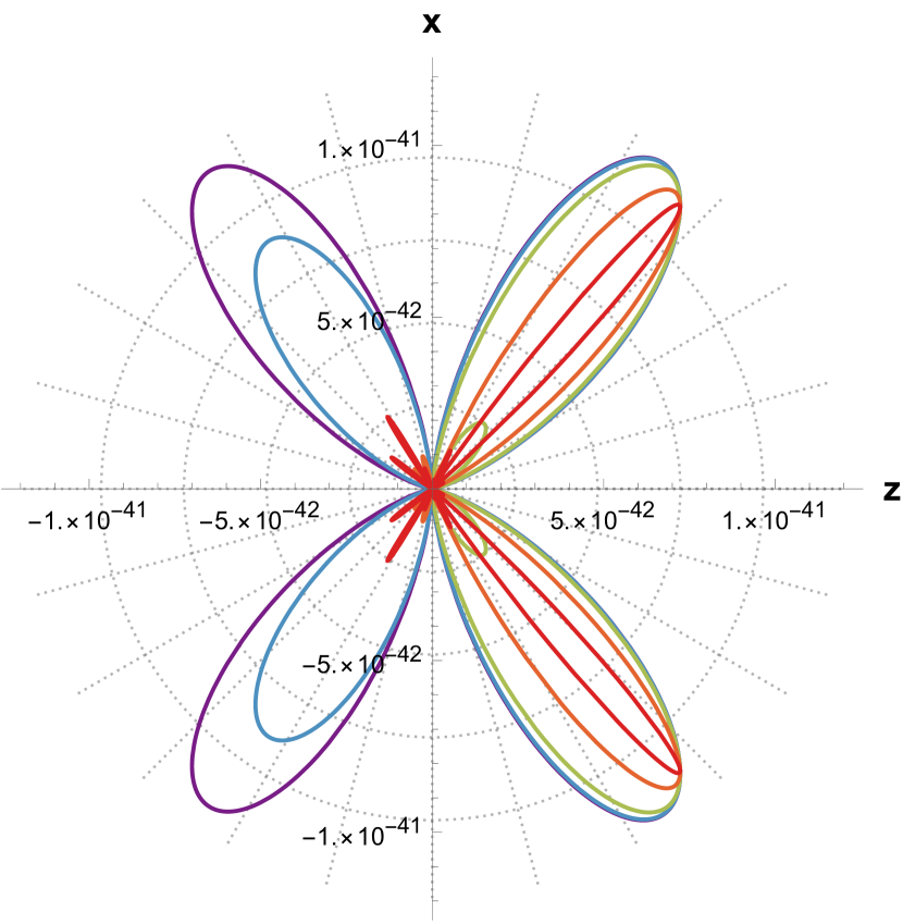
(a) $\bar{h}_{11}^{TT}(\theta)$

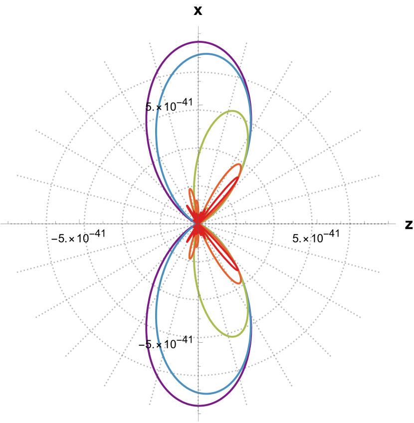
(b) $\bar{h}_{22}^{TT}(\theta)$

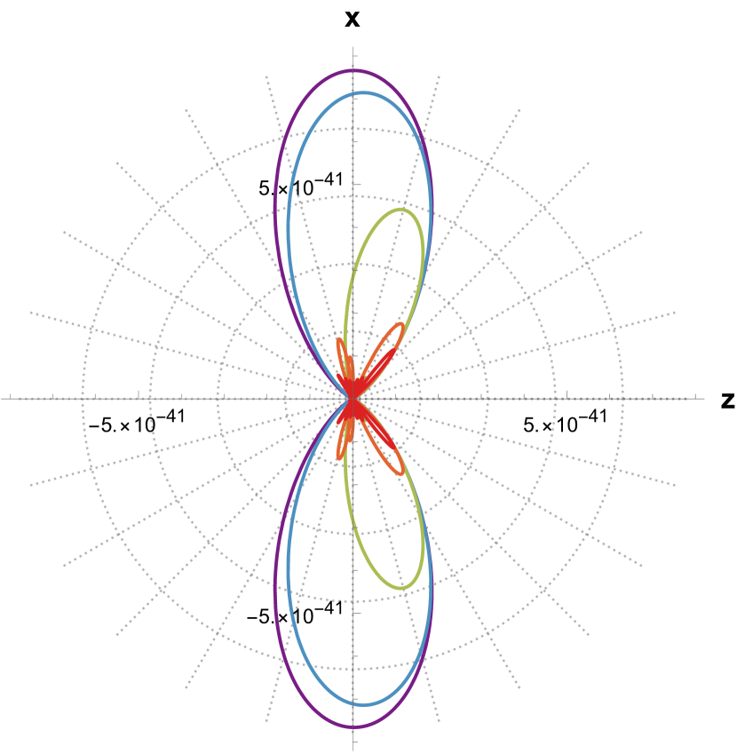
(c) $\bar{h}_{33}^{TT}(\theta)$

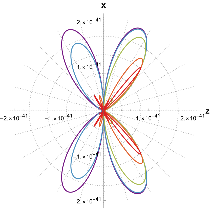
(d) $\bar{h}_{13}^{TT}(\theta)=\bar{h}_{31}^{TT}(\theta)$

Figure 5: Angular variation of the NIF ARC generated $l=0$ TT gauge metric perturbations ($\bar{h}_{\mu\nu}^{D,TT}+\bar{h}_{\mu\nu}^{ZZ,TT}$) in the $zx$ plane, one meter away from the source, for different values of the pulse frequency $\omega$, and hence of $\zeta_{L}$, and for $L=1$mm and $D=100\mu$m, such that $\zeta_{D}\leq 0.33$.

Figure 5 shows that, when $l=0$, no gravitational waves are emitted along the optical axis. Indeed, in the absence of orbital angular momentum, the energy distribution displays azimuthal symmetry in the plane perpendicular to the optical axis. Consequently, similarly to how oscillations of a symmetric mass distribution fail to generate gravitational waves, an observer positioned along the optical axis would not detect any gravitational radiation.

Interestingly, when $\zeta_{L}\geq 1$, $\text{Sinc}\left[\eta(\theta)\right]$ is evaluated outside of its central peak, leading to a noticeable reduction of the $\bar{h}_{D}+\bar{h}_{ZZ}$ angular distribution width. To maximise the signal, the condition $\zeta_{L}<1$ must be ensured.

Even more interestingly, those angular distributions exhibit a beaming effect when $\zeta_{L}$ becomes greater than one towards the angles $\theta_{\text{peak}}=\pm\alpha$, $\alpha$ being the half-cone angle introduced in figure 1. A Bessel beam can be thought as a linear superposition of plane waves which propagation directions are inclined at the half-cone angle $\alpha$ with respect to the $z$-axis. It is therefore not surprising that such plane waves generate metric perturbations whose amplitudes peak at $\theta_{\text{peak}}=\pm\alpha$.

V.1.4 Power emitted by gravitational waves ($l=0$)

The power per unit solid angle given in equation 19 contains all contractions of the radiative contributions and is a suitable observable to study. For $l=0$ it takes the form:

$$\small\text{$\frac{dP_{D}}{d\Omega}=g_{D}(\theta)F(\alpha)\mathcal{N}_{B}^{-2}\left(\omega_{g}^{l=0}\right)^{2}\frac{\pi GL^{2}P_{0}^{2}}{c^{7}}\Gamma^{2}_{0}(\theta)\text{Sinc}\left[\eta(\theta)\right]^{2}$}\leavevmode\nobreak\ ,$$ (85)

Where $P_{0}$ is the laser power and $g_{D}(\theta)$ and $F(\alpha)$ are respectively given by:

$$g_{D}(\theta) \equiv \frac{1}{16}\left[3-4\cos(2\theta)+\cos(4\theta)\right]\leavevmode\nobreak\ ,$$ (86)

$$F(\alpha) \equiv 2\left[1+\cos^{2}(\alpha)+\frac{1}{4}\sin^{2}(\alpha)\right]\leavevmode\nobreak\ .$$ (87)

This quantity is represented in figure 6, for the case of the NIF ARC facility. To improve graphical clarity in figure 6, different values of $\zeta_{L}$ were used to that in figure 5. Indeed, at constant laser power $P_{0}$, equation (85) exhibits that $dP_{D}/d\Omega\propto\omega_{g}^{2}$. The higher the frequency, the bigger the power radiated by gravitational waves (and the sizes of the lobes).

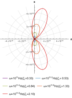
Figure 6: Angular distribution of the NIF ARC $\bar{h}_{D}+\bar{h}_{Z}$ generated gravitational radiation energy flux $dP_{D}/d\Omega$ in units of Watts from a Bessel mode with topological index $l=0$, for fixed values of $L=1$mm, $D=10\mu$m and $\beta=100\text{m}^{-1}$.

Also, and similarly to the $\bar{h}_{\mu\nu}^{TT}$ components represented in figure 5, a beaming effect towards the half-cone angle occurs for values of $\omega$ such that $\zeta_{L}>1$. Considering a detection system based on destructive measurements of the gravitational waves power using e.g. the inverse Gertsensthein effect, the location at which the greatest signal is detected depends on the pulse frequency.

V.2 Gravitational waves generated by a Bessel pulse with orbital angular momentum: $l=\pm 1$

The initial purpose of this study was to characterise the gravitational waves emitted by light carrying orbital angular momentum. To do so we consider from now on non-zero values of the OAM parameter $l$. As discussed earlier one can restrict the study to $l\in\left\{\pm 1\right\}$ as higher values lead to smaller amplitudes of the $\Gamma_{q}$ function. Also, using the following Bessel function identity $J_{-n}(x)=(-1)^{n}J_{n}(x),\;n\in\mathbb{Z},\;n\geq 0$ it can be shown that $\Gamma_{-q}=\Gamma_{q}$. Subsequent results are therefore invariant under this sign change of $q$.

Similarly to the $l=0$ case, gravitational waves described by the $\bar{h}_{D}$ and $\bar{h}_{ZZ}$ functions are still expected due to oscillations of the energy content in the source region. For $l=\pm 1$ this effect is however not dominant when compared to a new one: the twisting of the energy distributions described by the $\bar{h}_{+}$ and $\bar{h}_{\times}$ components. Indeed, when $l=\pm 1$, both $\bar{h}_{D}$ and $\bar{h}_{ZZ}$ contain $\Gamma_{1}$ functions and are therefore small compared to $\bar{h}_{+}$ and $\bar{h}_{\times}$ which contain $\Gamma_{0}$ functions through the $\bar{h}_{+}^{l\pm 1}$ and $\bar{h}_{\times}^{l\pm 1}$ contributions. The metric perturbation in the TT gauge is now well approximated by the sum of two distinct polarisations:

$$\bar{h}_{\mu\nu,l=\pm 1}^{TT}\simeq\bar{h}_{\mu\nu}^{+,TT}+\bar{h}_{\mu\nu}^{\times,TT}\leavevmode\nobreak\ .$$ (88)

V.2.1 Frequencies ($l=\pm 1$)

Similarly to the case with no orbital angular momentum, the frequency of the emitted gravitational waves is given by the function $\psi_{q}$ as it is the argument of the $\sin(\psi_{q})$ and $\cos(\psi_{q})$ functions appearing in equations (58) and (59). As for $l=0$, gravitational waves are therefore emitted at twice the frequency of the laser pulse:

$$\omega_{g}^{l=\pm 1}=2\omega\simeq 8.55\times 10^{14}\leavevmode\nobreak\ \text{Hz}\leavevmode\nobreak\ ,$$ (89)

For NIF’s 351 nm laser pulse [60]. The non-trivial equivalence between $\omega_{g}^{l=0}$ and $\omega_{g}^{l=\pm 1}$ will be further discussed section VI.

V.2.2 Amplitudes ($l=\pm 1$)

The amplitude of the associated gravitational waves is well estimated (once again up to the trigonometric functions entering the matrices in (75) and (76)) by the sum of the $\bar{h}_{+}$ and $\bar{h}_{\times}$ functions. Their maximal values over the $2\pi$ region in the $z-x$ plane are identical. One of them is represented on figure 7 as a function of the radial distance to the source, for different facilities for which we considered $L=c\tau_{p}/2$, as previously done.

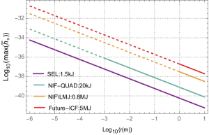
Figure 7: Plot of the peak gravitational wave strain for the optical parameters, $l=1$, $L=\tau_{p}/2$ and $D=10\mu m$, where ”$\tau_{p}$” is obtained from [12, 59]. We have included a potential next-generation (5 MJ, 250 TW) high-gain ICF laser facility called ”Future-ICF” in the data. Dashed lines denote when the radial distance ”r” falls below the range where the far-field approximation holds.

Those spacetime deformations do not exceed the $l=0$ case already presented in figure 4. Comparing those two figures, it appears that the twisting effect generates weaker spacetime deformations than the energy residual oscillations in the source volume in the absence of OAM. This strangeness is further discussed and justified in Appendix B. Interestingly, naive estimations are recovered as an equivalent system of rotating masses with effective masses $E_{L}/c^{2}\simeq 10^{-11}$ kg (1 MJ laser) separated by $\beta^{-1}=40$ nm and rotating at a frequency $\omega=5.37\times 10^{15}$ Hz would produce a strain $h\sim 6.4\times 10^{-38}$ one meter away from the source. This estimation is in very good agreement with figure 7. Obviously, more complex and subtle phenomena cannot be exhibited by this simple equivalence.

V.2.3 Angular distributions ($l=\pm 1$)

Figure 8 shows the angular distributions of the non-zero $\bar{h}_{\mu\nu}^{+,TT}$ and $\bar{h}_{\mu\nu}^{\times,TT}$ metric components one meter away from the source. One noticeable feature that differs from figure 5 is the appearance of gravitational waves emitted along the optical axis $z$. This discrepancy with respect to the previous $l=0$ case arises due to disruptions of the previous azimuthal symmetry by the presence of a non-zero topological index, giving rise to spiraling patterns in the energy density and gravitational waves along the optical axis. It is stressed here that this does not mean that those gravitational waves are longitudinal, their polarisations remain in the plane transverse to the direction of propagation.

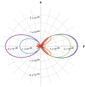
(a) $\bar{h}_{11}^{+,TT}(\theta)$

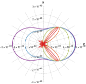
(b) $\bar{h}_{22}^{+,TT}(\theta)$

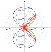
(c) $\bar{h}_{33}^{+,TT}(\theta)$

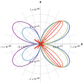
(d) $\bar{h}_{13}^{+,TT}(\theta)=\bar{h}_{31}^{+,TT}(\theta)$

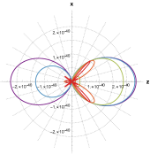
(e) $\bar{h}_{12}^{\times,TT}(\theta)=\bar{h}_{21}^{\times,TT}(\theta)$

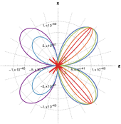
(f) $\bar{h}_{23}^{\times,TT}(\theta)=\bar{h}_{32}^{\times,TT}(\theta)$

Figure 8: Angular variation of the dominate NIF ARC generated $l=1$ TT gauge metric perturbations ($\bar{h}_{\mu\nu}^{+,TT}$ and $\bar{h}_{\mu\nu}^{\times,TT}$) in the $z-x$ plane, one meter away from the source, for different values of the pulse frequency $\omega$, and hence of $\zeta_{L}$ and for $L=1$mm and $D=100\mu$m, such that $\zeta_{D}\leq 0.33$.

As for all waves emitted in all but the direction corresponding to $\theta=\alpha$, those ”optical axis gravitational waves” are suppressed when $\zeta_{L}>1$ and the beaming effect towards the half-cone angle takes place.

V.2.4 Power emitted by gravitational waves ($l=\pm 1$)

The full metric perturbation being a linear superposition of independent $+$ and $\times$ polarisations, the power per unit solid angle of equation takes the form

$$dP/d\Omega\propto(g_{+}(\theta)\left<h_{+}^{2}\right>+g_{\times}(\theta)\left<h_{\times}^{2}\right>)\leavevmode\nobreak\ ,$$ (90)

With

$$g_{+}(\theta) \equiv \frac{\sin(\alpha)^{4}}{16}\left[19+12\cos(2\theta)+\cos(4\theta)\right]\leavevmode\nobreak\ ,$$ (91)

$$g_{\times}(\theta) \equiv \sin(\alpha)^{4}\left[1+\cos(2\theta)\right]\leavevmode\nobreak\ .$$ (92)

When $l=1$, the corresponding angular power distributions are:

$$\frac{dP_{+}}{d\Omega}=g_{+}(\theta)\mathcal{N}_{B}^{-2}\left(\omega_{g}^{l=1}\right)^{2}\frac{\pi GL^{2}P_{0}^{2}}{c^{7}}\Gamma_{l-1}^{2}(\theta)\text{Sinc}\left[\eta(\theta)\right]^{2}\leavevmode\nobreak\ ,$$ (93)

$$\frac{dP_{\times}}{d\Omega}=g_{\times}(\theta)\mathcal{N}_{B}^{-2}\left(\omega_{g}^{l=1}\right)^{2}\frac{\pi GL^{2}P_{0}^{2}}{c^{7}}\Gamma_{l-1}^{2}(\theta)\text{Sinc}\left[\eta(\theta)\right]^{2}\leavevmode\nobreak\ .$$ (94)

Figure 9 represents the power per unit solid angle of the $+$ polarised gravitational wave radiation. It is sufficient to represent only one polarisation mode as the angular distributions of the gravitational wave radiation flux for the $+$ and $\times$ polarisations are nearly identical, especially when $\zeta_{L}>1$. A more detailed comparison of both fluxes and their comparison with usual binary mergers radiated power is done in Appendix C.

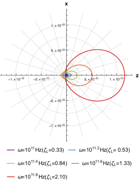
Figure 9: Angular distribution of the NIF ARC generated $h_{+}$ polarisation gravitational radiation energy flux $dP_{+}/d\Omega$ in units of Watts, from a Bessel mode with topological index $l=1$, for fixed values of $L=1mm$, $D=10\mu$m and $\beta=10^{6}\text{m}^{-1}$.

VI Discussion

What conclusions can be drawn from the results previously obtained?

Twisted lasers: the brightest sources of gravitational waves produced by humankind?

To know whether high energy lasers are the brightest sources of gravitational wave currently generated by humankind (or that could be generated in a near future) or not it is interesting to compare the previous amplitudes to the ones of gravitational waves emitted, e.g., by the orbital accelerator of the Spinlaunch project, which we estimated to be $h_{SL}\sim 10^{-36}$ at the optimistic distance of $10m$ to the source. This facility is probably among, if not the biggest, source of terrestrial gravitational waves produced by rotating masses. Even a 5 MJ laser pulse remains two orders of magnitude below (when the gravitational wave amplitude is evaluated at the same distance to the source). If a laser system could be constructed with energy comparable to the kinetic energy contained within the SpinLaunch system mass ($\sim 4.3\times 10^{8}$ J), the amplitude of the gravitational waves generated by Bessel modes would however become slightly bigger, $h\sim 10^{-35}$, still at $10m$ away from the source.

Does it mean that the game is over for high-energy lasers as sources of gravitational waves? Not necessarily, as their interest is manifold:

1. Beyond any possible technological application or measurable effect, the question of the gravitational field created by light is, in itself, fascinating and largely unexplored. A lot remains to be understood. This work provides new insights on the subtle properties of spacetime vibrations induced by coherent and monochromatic light.

2. The source volume is orders of magnitude smaller than the sub-orbital accelerators of the Spinlaunch project. As previously stated in this paper it might be that a detection system as the one proposed e.g., in [64], can be put (very) close to the source. The gravitational wave amplitude being $\propto 1/r$, this possibility might compensate the lacking orders of magnitude.

3. Twisted laser pulses allow for a better control of the gravitational wave properties such as their polarisation states and directions of emission. Thanks to a beam combiner it might even be possible to control their frequencies over a wide range. This possibility will be further explored in a subsequent study.

4. Twisted laser pulses may not be the highest sources of gravitational strains $h$ built by humankind, but they definitely are the highest sources of power radiated through gravitational waves, this quantity scaling with the square of the gravitational wave frequency: $dP_{D}/d\Omega\propto\omega_{g}^{2}$. Within the far-field approximation, the peak intensity of the SEL laser system at a distance equal to the laser pulse width and at $10m$ from the source are $9.4\times 10^{-5}\text{Wm}^{-2}$ and $1.9\times 10^{-17}\text{Wm}^{-2}$ respectively, which is many (18!) orders of magnitude greater than the estimated intensity of the Spinlaunch generated gravitational wave at the same distance of 10m from the source: $I_{SL}\sim 1.1\times 10^{-35}\text{Wm}^{-2}$. Interestingly, the intensity at the pulse boundary is one order of magnitude greater than the $3.6\times 10^{-6}\text{Wm}^{-2}$ intensity of the GW15094 signal [66] (measured at the detector location on earth).

Beaming

This study has revealed that gravitational waves emitted by Bessel mode laser pulses give rise to a beaming effect. The tilts and widths angular distributions presented, e.g., figures 5 or 8 depend significantly on the optical parameters, specifically through $\zeta_{D}\equiv\omega D/c$ and $\zeta_{L}\equiv\omega L/c$. When those parameters become greater than unity a beaming towards the half-cone angle $\alpha$ arises. This a priori non-trivial effect reflects properties of the Bessel pulse energy distributions function. If such waves could be detected one day, varying the optical parameters such as the pulse frequency or its time duration would have direct and important consequences on the signal.

Interestingly, this effect arises due to the non-zero spatial extension of the source. Indeed, when the laser pulse approaches a point source, the $\zeta_{L,D}$ parameters decrease to values for which the beaming does not occur anymore.

Gravitational wave frequencies

The gravitational waves explored in this paper are emitted at twice the pulse frequency, roughly around $10^{15}$ Hz.

The equivalence between $\omega_{g}^{l=0}$ and $\omega_{g}^{l=\pm 1}$, respectively given equations (83) and (89), might not be obvious at first sight as the sources of gravitational waves differ in both cases.

Indeed, in the absence of orbital angular momentum, gravitational waves are emitted due to oscillations of the energy content in the source region, oscillations whose frequency is twice the frequency of the fields (the energy simply being linked to the fields squared).

When $l=\pm 1$ the situation is different. Even though the previous effect still exists, the dominant source of gravitational waves is oscillations of the orbital angular momentum induced spirals in the energy density of the electromagnetic field. By examining the locations at which $\sin(\psi_{q})$ and $\cos(\psi_{q})$ vanish, corresponding to $\psi_{q}=p\pi$ and $\psi_{q}=(2p+1)\pi/2,\leavevmode\nobreak\ p\in\mathbb{Z},\;p\geq 0$ respectively, it can be inferred that the number of rotating lobes in the interval $\phi\in[0,2\pi]$ is twice the value of the topological index. Moving on to the temporal evolution of a constant phase point in a plane defined by $z=$constant, it can be demonstrated from $\partial\psi_{q}/\partial t=0$ that the rotational frequency of each lobe in a laser with frequency $\omega$ is $\omega/l$. Nevertheless, the frequency at which the system reproduces identically is dictated by the multiplication of the individual frequency and the number of lobes, yielding an exact frequency of $2\omega$ whatever the value of $\l$. Notably, and interestingly, $\omega_{g}$ is independent of the topological index.

Those gravitational wave frequencies are many orders of magnitude above the astrophysical standards. Indeed, no substantial gravitational wave signals are normally expected above a few kHz, the upper bound being given by the ringdown phase of neutron stars mergers [22, 67].

High frequency gravitational waves are however also expected from many beyond standard model sources, such as mergers or evaporation of light primordial black holes [68, 69, 70, 71], superradiance phenomena [72, 73, 74, 75], collisions of ”bubbles” arising from phase transitions in the early universe [76, 77, 78], topological defects such as cosmic strings [79, 80, 81, 82], etc. Some of these sources can lead to gravitational waves well above the kHz range. An excellent review of gravitational waves in the MHz-GHz range can be found in [22]. However, barring primordial black holes, those sources hardly go above the $10^{12}-10^{13}$ Hz, even in the most extreme scenarios. Only light black holes of primordial origin could emit gravitational waves at frequencies comparable or even greater than laser-generated gravitational waves.

Detection

There is not yet a final word on the best way to search for gravitational waves at very high frequencies. The most promising possibility might not be by direct measurement of the strain but through the inverse Gertsenshtein effect [84], i.e. the (resonant) conversion of gravitational waves into photons in the presence of (static) electromagnetic fields. The conversion into photons has been [85, 86, 87] and still is [22, 88, 89] studied frequently: in cosmology [90, 91, 92, 93, 94], and more recently in the context of haloscopes and resonant cavities [95, 96, 97, 98]. This method takes advantage of the high values of the gravitational wave frequencies. As an example, the effective current generated by the conversion of a gravitational wave in a GHz resonant cavity scales with the square of the gravitational wave frequency [95].

For $10^{16}$ Hz gravitational waves, the possibility to use high-energy lasers as detectors has also recently been considered [64]. In this paper the authors have investigated the feasibility of employing high-energy laser pulses as gravitational wave detectors, considering a laser pulse with an energy of 1.8 MJ. In their most optimistic scenario, they determined that a sensitivity level of $10^{-27}$ could be attained. This value, already extremely impressive in itself, remains orders of magnitude above that required one to detect laser-produced gravitational waves. However, given that laser pulses can be focused to incredibly small spot sizes, they probably offer the most viable pathway for probing the emitted gravitational waves at the required length scales. In a broader context, they offer a unique possibility to probe gravitational waves at extremely high frequencies, around $10^{16}$ Hz. Further exploration of this detection method will be performed in a subsequent work.

How to maximise the signal?

What optical parameters influence the maximal gravitational wave amplitudes generated by a Bessel pulse?

Looking at equations (56) and (57) and putting the trigonometric functions depending on $\psi_{q}$ apart, four different functions must a priori play a role: $\bar{h}_{0}(r)$, the trigonometric functions in the half cone angle $\alpha$, $\Gamma_{0}$ and $\text{Sinc}\left[\eta(\theta)\right]$.

At fixed distance $r$ to the source, those functions depend on the following optical parameters: the pulse energy $\mathcal{E}$, its frequency $\omega$, its duration $\tau_{P}$, its half cone angle $\alpha$, its confinement diameter $D$ and its beam waist $\beta$.

Pulse energy $\mathcal{E}$: As shown in figures 4 and 7, spacetime deformations increase with the pulse energy. The intuitive scaling of the gravitational effect with the energy is recovered: the greater the energy, the bigger the maximal strain. The energy appears in $\bar{h}_{0}$. Indeed, at fixed $r$ and $\beta$, maximising this function is equivalent to maximise $E_{0}^{2}L/\beta^{2}$, i.e. the pulse power times its length, which is the pulse energy.

Higher energy pulses generate larger spacetime deformations. Does this mean that the most energetic laser pulses automatically are the most interesting sources from the point of view of an observer trying to detect them? Not necessarily as, ideally, for lower energy lasers such as the SEL 1.5 kJ pulse, a detection system could be placed closer to the source. Depending on how close one can get to the source, considering lower energy pulses might be favored.

Pulse duration $\tau_{P}$: The pulse duration appears in the $\text{Sinc}\left[\eta(\theta)\right]$ function, as $\eta(\theta)=\zeta_{L}\left[\cos(\theta)-\cos(\alpha)\right]$ with $L=c\tau_{P}$. For the Sinc function to be at unity, it needs to be evaluated close to the maximum of its central peak. For this to be the case whatever the value of $\theta$, the criterion $\zeta_{L}\equiv\omega L/c<1\Leftrightarrow\tau_{P}<\omega^{-1}\Leftrightarrow\tau_{P}<10^{-15}$s for a $10^{15}$ Hz pulse, must be satisfied. Due to the diffraction limit such values are not easy to reach in practice but $\zeta_{L}\approx 10$ is a reasonable assumption (ten femtoseconds lasers pulses) [65, 59]. Once $\zeta_{L}<1$ is satisfied there is no need in diminishing the pulse duration.
The current minimum duration of laser pulses in peta-Watt laser systems typically ranges from a few tens to a few hundred femtoseconds. However, this duration can often surpass the limit imposed by a single optical cycle, which is on the order of $\lambda/c$ [99, 100]. For a laser with a central wavelength of $351$ nm, the pulse width constrained by a single optical cycle is $1.17$ fs, for which $\zeta_{L}=2\pi$. To enable the development of lasers operating in the exa-Watt regime [55] various techniques have been devised to compress laser pulses to the limit of a single optical cycle [101, 102, 103]. A comprehensive review of these techniques can be found in [59, 65].

Confinement diameter $D$ and beam waist $\beta$: The beam waist $\beta$ does not exist as an independent parameter. Rather, its value is intricately linked to both the wavelength of light and the desired half-cone angle and is constrained by the diffraction limit. On the other hand, the confinement diameter $D$ maintains its status as an independent parameter. However, it must adhere to the condition $D\geq\beta^{-1}$.

As previously discussed and as shown in figure 3, max$\left(\Gamma_{0}\right)$ is independent of $\zeta_{D}\equiv\omega D/c$. Varying the diameter of the source cylinder has no effect on the maximal value of $\Gamma_{0}$, nor does a variation in the pulse frequency $\omega$. As shown in Appendix A the angular distribution of $\Gamma_{0}$ however depends on $\zeta_{D}$. Similarly to the Sinc function, for $\Gamma_{0}$ to take its maximal value whatever $\theta\in\left[0;2\pi\right]$ the condition $\zeta_{D}<1$ must be fulfilled, i.e. $D$ must be lower than $\lambda/(2\pi)\simeq 55.9$ nm for a NIF’s 351 nm beam.

The fact that $\beta$ and $D$ must be decreased in order to boost the signal is somehow counter intuitive when making an analogy with massive binary systems, for which the distance between the two bodies increases the lever arm and thus the gravitational strain. The origin of this discrepancy is mainly twofold. First, the expansion of the retarded time to linear order accounts for the non-zero size of the laser pulse. Second, both the amplitude and the phase exhibit inherent variations at each point within the laser pulse. The difference between gravitational waves emitted by laser pulses and massive binary systems becomes more and more pronounced as the values of $\zeta_{D}$ and $\zeta_{L}$ increase above one, for which the laser pulse increasingly deviates from resembling a point source.

Half cone angle $\alpha$: The value of $\alpha$ cannot be fixed such that all four $\bar{h}_{D}$, $\bar{h}_{ZZ}$, $\bar{h}_{+}^{(Q)}$ and $\bar{h}_{x}^{(Q)}$ equations (56 - 59) are simultaneously maximised. In order to maximise the highest number of them the maximal reachable value $\alpha_{\text{max}}=0.848\simeq\pi/3.7$ rads [45] has been considered.

Pulse frequency $\omega$: Since for photons $E=\hbar\omega$, we could expect a linear increase of the gravitational strain with the photon frequency. However laser facilities deliver a fixed energy. Writing $E_{0}^{2}\sim n\hbar\omega/\epsilon_{0}c$, with $n$ the photon number density, varying the frequency $\omega$ by processes such as second harmonic generation [104] results in diminishing the photon number density $n$ (or vice versa) so that the total pulse energy remains unchanged. Therefore, once the pulse energy is fixed and the conditions $\tau_{P}<\omega^{-1}$ and $D<c/\omega$ are satisfied, the pulse frequency plays no role in the amplitudes of the emitted gravitational waves. However the power radiated by gravitational waves scales quickly with $\omega$, as $dP_{D}/d\Omega\propto\omega^{2}$. Increasing the frequency is a promising way to increase the gravitational wave power. This effect is highly important as detection through the inverse Gertsensthein effect relies on this power.

In summary, to maximise the gravitational waves signal at fixed distance $r$ to the source:

• The pulse energy needs to be maximised;

• At fixed pulse energy, the pulse frequency does not affect the strain, but its increase is of primary importance for the power;

• The pulse duration needs to be small enough such that $\tau_{P}<\omega^{-1}$. Once this condition is fulfilled the pulse duration no longer matters. For the beaming effect to be enhanced, however, $\tau_{P}>\omega^{-1}$ and the longer the pulse, the bigger the beaming;

• The confinement diameter and waist need to be small enough such that $D<\lambda/(2\pi)$. Once this condition is fulfilled the confinement diameter no longer matters.

• The half cone angle $\alpha$ needs to be increased, but its impact is of secondary importance.

VII Conclusion

The understanding of the detailed structure of the gravitational field produced by light is still in its infancy. In this work, the characteristics of gravitational waves produced by Bessel pulses have been extensively investigated for the first time. Analytical formulations and numerical evaluations of the spacetime deformations and the associated power have been provided. The influence of the different optical parameters on the signal has also been discussed in detail. In addition, the parameters of interest required to boost the signal amplitude have been made explicit.

Notably, a deeply non-intuitive angular distribution of the signal has been found, revealing fascinating subtleties of spacetime deformations generated by high-power laser pulses. This exemplifies how different laser-generated gravitational waves are from textbook signals, e.g. those generated in astrophysical binary systems of compact objects. Most of the complex patterns found in this study do not exist at all when considering basic rotating masses.

Many paths remain to be explored, among which:

1. Laguerre-Gaussian pulses are another class of twisted light pulses, often considered in applications. The gravitational waves generated by this second class of pulses with orbital angular momentum might reveal new aspects of gravitational radiation physics.

2. Multi-beam interactions via beam combiners could facilitate the generation of gravitational waves at the beat frequency of the stress-energy distribution. Theoretically, using modern optical techniques, this could allow for the emission of gravitational waves in the MHz to GHz range. This could be of high interest for other detection methods, such as resonant cavities.

3. A laboratory control of gravitational waves may also be useful to probe parametric resonant effects that require high levels of tuning. Notably, in [105], it has been shown that gravitational waves can excite a parametric resonant instability of the electromagnetic field, improving graviton to photon conversion. The inverse process, namely the exponential enhancement of the gravitational wave signal via parametric resonance, can also occur for standing electromagnetic waves in vacuum. This possibility is currently under investigation.

4. The group velocity of Bessel modes is not necessarily equal to the speed of light. Subluminal Bessel pulses may exhibit a Doppler effect in the generated gravitational wave signal which has the potential to influence its intensity, angular distribution, and time duration.

All those possibilities will be considered in subsequent studies.

Beyond any mastering of laboratory controlled gravitational waves, which would undoubtedly lead to a scientific revolution, it is already remarkable in itself that the richness – and complexity – of gravitational radiation physics that extends past elementary situations slowly reveals itself in its intricacy.

VIII Acknowledgements

The authors gratefully acknowledge useful discussions with Prof. Gianluca Gregori, Prof. Robert Bingham, Dr. Raoul Trines, Professor Steven Balbus, Mr. Georgios Vacalis and Dr Robert Kirkwood. They also thank all of the staff of the Central Laser Facility, Rutherford Appleton Laboratory for their assistance in the development of this work. The work was supported by the Oxford-ShanghaiTech collaboration agreement and UKRI-STFC grant ST/V001655/1. The work of C.L. was supported by the grants 2018/30/Q/ST9/00795 and 2021/42/E/ST9/00260 from the National Science Centre (Poland).

Appendix A Angular distribution of $\Gamma_{l}(\theta)$

To study the angular distribution of the emitted gravitational waves one first focuses on the study of the two functions that impact a priori the direction of emission of gravitational waves in the $zx$ plane:

• $\text{Sinc}\left[\eta(\theta)\right]$;

• and $\Gamma_{l}^{BP}(\theta)$.

The angular dependence of $\Gamma_{l}^{BP}(\theta)$ is entirely governed by the $J_{2l}\left[\omega\tau\sin(\theta)/c\beta\right]$ factor within equation (53).

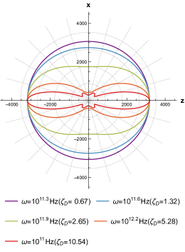
Figure 10: Angular variation of $\Gamma_{0}(\theta)$ in the $zx$ plane, for $\theta\in\left[0;2\pi\right[$ and for different values of the pulse frequency $\omega$, hence of $\zeta_{D}$, with fixed value of $D=0.1$mm.

In figure 3 we have stated that the dominant $\Gamma_{q}$ function is $\Gamma_{0}(\theta)$ and that its maximal value, occurring along the optical axis when $\theta=0$, is independent of $\zeta_{D}$, hence of the cylinder diameter. Figure 10 represents the variation of $\Gamma_{0}(\theta)$ for $\theta\in\left[0;2\pi\right[$, keeping the size of the cylinder given by $L$ and $D$ fixed, but varying the frequency (which induces variations of $\zeta_{D}$). For values of $\zeta_{D}>1$ a beaming effect starts to appear along the direction of propagation of the pulse. This beaming leads to a decrease of $\Gamma_{0}(\theta)$ off z-axis, and thus a decrease of the emitted waves amplitudes off optical axis. To prevent the emergence of this effect it is preferable to work with $\zeta_{D}<1$. At fixed frequency, it means considering a cylinder diameter such that $D<c/\omega$.

An increase of $\zeta_{D}$ induces an increase of $\Gamma_{q\neq 0}$ functions, as depicted in figure 3. Unlike $\Gamma_{0}$ the maximal values of all other $\Gamma_{q\neq 0}$ and the angles $\theta$ at which they occur depend on $\zeta_{D}$. Indeed, Consider some threshold $\zeta_{D}^{th}$ which value depends on $q$. For $q=0$, $\zeta_{D}^{th}\simeq 1$ but for $q\neq 0$ the threshold must be computed numerically. For all values $\zeta_{D}\leq\zeta_{D}^{th}$ the maxima of the $\Gamma_{q\neq 0}$ lie along the x-axis. However, when $\zeta_{D}>\zeta_{D}^{th}$, the location of the maxima of $\Gamma_{q\neq 0}$ vary and need to be evaluated numerically. As an example, the case of $q=1$ has been depicted in figure 11.

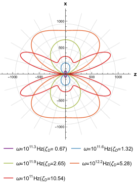
Figure 11: Angular variation of $\Gamma_{1}(\theta)$ in the $zx$ plane, for $\theta\in\left[0;2\pi\right[$ and for different values of the pulse frequency $\omega$, hence of $\zeta_{D}$, with fixed value of $D=0.1$mm.

Obviously $\Gamma_{0}$ does not remain the dominant function for all values of $\theta$ and $\zeta_{D}$. For this function to remain overwhelmingly dominant whatever the direction around the source, rendering all the other generated $\Gamma_{q},\leavevmode\nobreak\ q\neq 0,$ negligible, one needs to stay in the regime $\zeta_{D}<\zeta_{D}^{th}$, for which $\zeta_{D}^{th}>1$ if $q\neq 0$.

This effect arises due to the way the source volume is defined. At fixed values of $\beta$ and $\omega$, increasing the cylinder diameter $D$ increases the number of lobes of the Bessel pulse that act as sources of gravitational waves. Since for Bessel pulses the energy is split equally between the lobes [50, 32, 33], more lobes in the cylinder result in smaller peak intensity in each lobe, thus in smaller gravitational waves amplitudes.

Appendix B Why is twisting not the dominant effect generating gravitational waves in Bessel pulses?

How is it that the twisting effect is not dominant in the generation of gravitational waves? To better understand this question, the Maxwell tensor is first discussed in more detail.

The Maxwell tensor serves as a mathematical representation of the ”pressure” and ”shear stress” exerted on the surrounding spacetime by electromagnetic waves.

In the case of a sole electromagnetic wave, these stresses are aligned, when acting on a physical object, with the momentum of the wave. For a single plane wave this direction corresponds to its direction of propagation. Without loss of generality and as we did, it is possible to align the z-axis along the propagation direction of the plane wave. In this scenario, the only non-zero component of the Maxwell tensor is $\sigma_{zz}$, indicating the presence of pressure along the z-axis.

To generate additional pressure and shear stress components in the Maxwell tensor, the interaction of multiple electromagnetic plane waves propagating at angles to each other is necessary. When multiple plane waves interact, the resulting electromagnetic field distribution can give rise to non-zero components of the Maxwell tensor beyond $\sigma_{zz}$.

The electromagnetic wave field tensors of two plane waves propagating at an angle $2\Theta$ to each other in the $xz$ plane, described by the 4-wavevectors $K^{\mu}_{\pm}\equiv\left[\omega/c,\pm k\sin(\Theta),0,k\cos(\Theta)\right]$ are given by:

$$\frac{\mathcal{F}^{\mu\nu}_{\pm}(\Theta)}{C_{\pm}}=\begin{pmatrix}0&-\cos(\Theta)&0&\pm\sin(\Theta)\\ \cos(\Theta)&0&0&1\\ 0&0&0&0\\ \mp\sin(\Theta)&-1&0&0\end{pmatrix}\leavevmode\nobreak\ ,$$ (95)

where $C_{\pm}\equiv(E_{0}/c)\cos(K^{\pm}_{\mu}x^{\mu})$. The Maxwell tensor resulting from their interaction is:

$$\sigma_{xx}=\frac{1}{2}\epsilon_{0}c^{3}\sin(\Theta)^{2}(B^{2}-A^{2})\leavevmode\nobreak\ ,$$ (96)

$$\sigma_{yy}=-\sigma_{xx}\leavevmode\nobreak\ ,$$ (97)

$$\sigma_{zz}=-\frac{1}{2}\epsilon_{0}c^{3}\left((1+\cos(\Theta)^{2})A^{2}+\sin(\Theta)^{2}B^{2}\right)\leavevmode\nobreak\ ,$$ (98)

$$\sigma_{xz}=-\frac{1}{2}\epsilon_{0}c^{3}\sin(2\Theta)AB\leavevmode\nobreak\ ,$$ (99)

$$\sigma_{xy}=0\leavevmode\nobreak\ ,$$ (100)

$$\sigma_{yz}=0\leavevmode\nobreak\ .$$ (101)

Where $A$ and $B$ are $C_{+}+C_{-}$ and $C_{+}-C_{-}$ respectively. The resulting amplitude of the oscillatory components $\tilde{\sigma}_{xx}$ and $\tilde{\sigma}_{zz}$ of the Maxwell tensor for this system at $x=0$ are given by $\tilde{\sigma}_{xx}(\Theta)=\epsilon_{0}E_{0}^{2}\sin^{2}(\Theta)$ and $\tilde{\sigma}_{zz}=\epsilon_{0}\left(E_{0}^{2}/2\right)(1-\cos(2\Theta)-4)$ respectively. Within the domain $\Theta\in[0,\pi/2]$, $|\tilde{\sigma}_{xx}(\Theta)|<|\tilde{\sigma}_{zz}(\Theta)|$. This reasoning can be generalised to the case of an Bessel mode which is an infinite superposition of plane waves. The difference for Bessel modes is that they can exhibit a twist in the field such that it produces shear stresses on the surounding spacetime that give rise to $\bar{h}_{xy}$, unlike the case of two interacting plane waves which only produce outward pressure. Thus in contrast to the $\sigma_{zz}$ component of the Maxwell tensor, the components $\sigma_{ab}$, $a,b\in\left\{x,y\right\}$ exhibit growth with increasing tilt angle between the corresponding electromagnetic waves. Since a Bessel mode can be regarded as an infinite superposition of plane waves with a characteristic angle of inclination $\alpha$ between them, the amplitude of the generated $+$ and $\times$ polarized gravitational waves is lower than that of the gravitational waves generated by the $\sigma_{ab}^{D}$ and $\sigma_{ab}^{ZZ}$ terms of the Maxwell tensor.

Appendix C Comparison of the $+$ and $\times$ angular power distributions radiated in the $l=1$ case.

In most of the cases represented in Figure 9 $\zeta_{L}>1$ and the angular distributions of the power associated with $+$ and $\times$ polarisations are hardly distinguishable. A small difference begins to appear along the $x$ axis for values of $\zeta_{L}<1$, as shown figure 12, but both power distributions remain extremely close for most values of the angle $\theta$ in the $zx$ plane.

In addition, from De Moivre’s theorem, it can be demonstrated that the sum $g_{+}(\theta)+g_{\times}(\theta)$ is proportional to the angular distribution of gravitational wave radiation emitted by a binary merger [23]. Consequently, when $\zeta_{L}<1$, the envelope of gravitational waves generated by the Bessel pulse exhibits an identical pattern to those emitted by a binary merger. However, due to the expansion of the retarded time to linear order in the source dimensions, deviations from this distribution occur as the Bessel pulse deviates from a point source ($\zeta_{L}>1$).

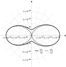
Figure 12: Angular distribution of the NIF ARC generated gravitational radiation energy flux for $\zeta_{L}=0.33$ and for fixed values of $L=1mm$, $D=10\mu$m.

References

- Weber [1960] J. Weber, Detection and generation of gravitational waves, Phys. Rev. 117, 306 (1960).
- Halpern and Laurent [1964] L. Halpern and B. Laurent, On the gravitational radiation of microscopic systems, Il Nuovo Cimento 33, 728 (1964).
- Grishchuk and Sazhin [1974] L. Grishchuk and M. Sazhin, Emission of gravitational waves by an electromagnetic cavity, Journal of Experimental and Theoretical Physics - J EXP THEOR PHYS 38 (1974).
- Grishchuk and Sazhin [1975] L. P. Grishchuk and M. V. Sazhin, Excitation and detection of standing gravitational waves, Zhurnal Eksperimentalnoi i Teoreticheskoi Fiziki 68, 1569 (1975).
- Grishchuk [1977] L. P. Grishchuk, Gravitational waves in the cosmos and the laboratory, Soviet Physics Uspekhi 20, 319 (1977).
- Grishchuk [2003] L. P. Grishchuk, Electromagnetic generators and detectors of gravitational waves, in 1st Conference on High Frequency Gravitational Waves (2003) arXiv:gr-qc/0306013 .
- Kolosnitsyn and Rudenko [2015] N. I. Kolosnitsyn and V. N. Rudenko, Gravitational Hertz experiment with electromagnetic radiation in a strong magnetic field, Phys. Scripta 90, 074059 (2015), arXiv:1504.06548 [gr-qc] .
- Faccio et al. [2006] D. Faccio, M. Clerici, and D. Tambuchi, Revisiting the 1888 Hertz experiment, American Journal of Physics 74, 992 (2006), arXiv:physics/0602073 [physics.ed-ph] .
- Morozov et al. [2021] A. N. Morozov, V. I. Pustovoit, and I. V. Fomin, Generation of Gravitational Waves by a Standing Electromagnetic Wave, Gravitation and Cosmology 27, 24 (2021).
- Tolman et al. [1931] R. C. Tolman, P. Ehrenfest, and B. Podolsky, On the gravitational field produced by light, Phys. Rev. 37, 602 (1931).
- M. E. Gertsenshtein [1962] M. E. Gertsenshtein, Wave resonance of light and gravitional waves, Journal of Experimental and Theoretical Physics 41, 113 (1962).
- Danson et al. [2019] C. N. Danson, C. Haefner, J. Bromage, T. Butcher, J.-C. F. Chanteloup, E. A. Chowdhury, A. Galvanauskas, L. A. Gizzi, J. Hein, D. I. Hillier, N. W. Hopps, Y. Kato, E. A. Khazanov, R. Kodama, G. Korn, R. Li, Y. Li, J. Limpert, J. Ma, C. H. Nam, D. Neely, D. Papadopoulos, R. R. Penman, L. Qian, J. J. Rocca, A. A. Shaykin, C. W. Siders, C. Spindloe, S. Szatmári, R. M. G. M. Trines, J. Zhu, P. Zhu, and J. D. Zuegel, Petawatt and exawatt class lasers worldwide, High power laser science and engineering 7, e54 (2019).
- Rätzel et al. [2016] D. Rätzel, M. Wilkens, and R. Menzel, Gravitational properties of light—the gravitational field of a laser pulse, New Journal of Physics 18, 023009 (2016).
- Scully [1979] M. O. Scully, General-relativistic treatment of the gravitational coupling between laser beams, Phys. Rev. D 19, 3582 (1979).
- Lageyre et al. [2022] P. Lageyre, E. d’Humières, and X. Ribeyre, Gravitational influence of high power laser pulses, Phys. Rev. D 105, 104052 (2022).
- Ng and Ooi [2013] K. S. Ng and C. H. R. Ooi, Weak gravitational field of Bessel beam, AIP Conference Proceedings 1528, 456 (2013), https://pubs.aip.org/aip/acp/article-pdf/1528/1/456/12204645/456_1_online.pdf .
- Schneiter et al. [2018] F. Schneiter, D. Rätzel, and D. Braun, The gravitational field of a laser beam beyond the short wavelength approximation, Classical and Quantum Gravity 35, 195007 (2018).
- McGloin and Dholakia [2005] D. McGloin and K. Dholakia, Bessel beams: Diffraction in a new light, Contemporary Physics 46, 15 (2005), https://doi.org/10.1080/0010751042000275259 .
- Volke-Sepulveda et al. [2002] K. Volke-Sepulveda, V. Garcés-Chávez, S. Chávez-Cerda, J. Arlt, and K. Dholakia, Orbital angular momentum of a high-order bessel light beam, Journal of Optics B: Quantum and Semiclassical Optics 4, S82 (2002).
- Gomes and Rovelli [2023] H. Gomes and C. Rovelli, On the analogies between gravitational and electromagnetic radiative energy, (2023), arXiv:2303.14064 [physics.hist-ph] .
- Buonanno and Sathyaprakash [2015] A. Buonanno and B. S. Sathyaprakash, Sources of gravitational waves: Theory and observations, in General Relativity and Gravitation: A Centennial Perspective, edited by A. Ashtekar, B. K. Berger, J. Isenberg, and M. MacCallum (Cambridge University Press, 2015) p. 287–346.
- Aggarwal et al. [2021] N. Aggarwal et al., Challenges and opportunities of gravitational-wave searches at MHz to GHz frequencies, Living Rev. Rel. 24, 4 (2021), arXiv:2011.12414 [gr-qc] .
- Maggiore [2007] M. Maggiore, Gravitational Waves. Vol. 1: Theory and Experiments, Oxford Master Series in Physics (Oxford University Press, 2007).
- Eddington [1922] A. S. Eddington, The propagation of gravitational waves, Proceedings of the Royal Society of London. Series A, Containing Papers of a Mathematical and Physical Character 102, 268 (1922).
- Éanna É Flanagan and Hughes [2005] Éanna É Flanagan and S. A. Hughes, The basics of gravitational wave theory, New Journal of Physics 7, 204 (2005).
- Lifshitz [2017] E. Lifshitz, Republication of: On the gravitational stability of the expanding universe, General Relativity and Gravitation 49, 10.1007/s10714-016-2165-8 (2017).
- Bertschinger [2000] E. Bertschinger, Cosmological perturbation theory and structure formation (2000), arXiv:astro-ph/0101009 [astro-ph] .
- Hobson et al. [2006] M. P. Hobson, G. Efstathiou, and A. N. Lasenby, General relativity: An introduction for physicists (Cambridge University Press, 2006).
- Allen and Padgett [2011] L. Allen and M. Padgett, The orbital angular momentum of light: An introduction, in Twisted Photons (John Wiley and Sons, Ltd, 2011) Chap. 1, pp. 1–12.
- Allen et al. [1992a] L. Allen, M. W. Beijersbergen, R. J. C. Spreeuw, and J. P. Woerdman, Orbital angular momentum of light and the transformation of laguerre-gaussian laser modes, Phys. Rev. A 45, 8185 (1992a).
- Barnett and Allen [1994] S. M. Barnett and L. Allen, Orbital angular momentum and nonparaxial light beams, Optics Communications 110, 670 (1994).
- Durnin [1987] J. Durnin, Exact solutions for nondiffracting beams. i. the scalar theory, J. Opt. Soc. Am. A 4, 651 (1987).
- Durnin et al. [1987] J. Durnin, J. J. Miceli, and J. H. Eberly, Diffraction-free beams, Phys. Rev. Lett. 58, 1499 (1987).
- Quinteiro et al. [2015] G. F. Quinteiro, D. E. Reiter, and T. Kuhn, Formulation of the twisted-light–matter interaction at the phase singularity: The twisted-light gauge, Phys. Rev. A 91, 033808 (2015).
- Jackson [1999] J. D. Jackson, Classical electrodynamics, 3rd ed. (Wiley, New York, NY, 1999).
- Allen et al. [1992b] L. Allen, M. W. Beijersbergen, R. J. C. Spreeuw, and J. P. Woerdman, Orbital angular momentum of light and the transformation of laguerre-gaussian laser modes, Phys. Rev. A 45, 8185 (1992b).
- Aboushelbaya et al. [2019] R. Aboushelbaya, K. Glize, A. F. Savin, M. Mayr, B. Spiers, R. Wang, J. Collier, M. Marklund, R. M. G. M. Trines, R. Bingham, and P. A. Norreys, Orbital angular momentum coupling in elastic photon-photon scattering, Phys. Rev. Lett. 123, 113604 (2019).
- Denoeud et al. [2017] A. Denoeud, L. Chopineau, A. Leblanc, and F. Quéré, Interaction of ultraintense laser vortices with plasma mirrors, Phys. Rev. Lett. 118, 033902 (2017).
- Shi et al. [2022] Y. Shi, D. R. Blackman, P. Zhu, and A. Arefiev, Electron pulse train accelerated by a linearly polarized laguerre–gaussian laser beam, High Power Laser Science and Engineering 10, e45 (2022).
- Zhang et al. [2022] L. Zhang, L. Ji, and B. Shen, Intense harmonic generation driven by a relativistic spatiotemporal vortex beam, High Power Laser Science and Engineering 10, e46 (2022).
- Shi et al. [2018] Y. Shi, J. Vieira, R. M. G. M. Trines, R. Bingham, B. F. Shen, and R. J. Kingham, Magnetic field generation in plasma waves driven by copropagating intense twisted lasers, Phys. Rev. Lett. 121, 145002 (2018).
- Mirhosseini et al. [2013] M. Mirhosseini, M. Malik, Z. Shi, and R. W. Boyd, Efficient separation of the orbital angular momentum eigenstates of light, Nature Communications 4, 2781 (2013).
- Krenn et al. [2014] M. Krenn, R. Fickler, M. Fink, J. Handsteiner, M. Malik, T. Scheidl, R. Ursin, and A. Zeilinger, Communication with spatially modulated light through turbulent air across vienna, New Journal of Physics 16, 113028 (2014).
- Lei et al. [2017] T. Lei, S. Gao, Z. Li, Y. Yuan, Y. Li, M. Zhang, G. N. Liu, X. Xu, J. Tian, and X. Yuan, Fast-switchable oam-based high capacity density optical router, IEEE Photonics Journal 9, 1 (2017).
- Khonina et al. [2021] S. N. Khonina, N. L. Kazanskiy, P. A. Khorin, and M. A. Butt, Modern types of axicons: New functions and applications, Sensors 21, 10.3390/s21196690 (2021).
- Chen et al. [2020] R. Chen, H. Zhou, M. Moretti, X. Wang, and J. Li, Orbital angular momentum waves: Generation, detection, and emerging applications, IEEE Communications Surveys & Tutorials 22, 840 (2020).
- Wei et al. [2015] X. Wei, C. Liu, L. Niu, Z. Zhang, K. Wang, Z. Yang, and J. Liu, Generation of arbitrary order bessel beams via 3d printed axicons at the terahertz frequency range, Appl. Opt. 54, 10641 (2015).
- Boucher et al. [2018] P. Boucher, J. D. Hoyo, C. Billet, O. Pinel, G. Labroille, and F. Courvoisier, Generation of high conical angle bessel–gauss beams with reflective axicons, Appl. Opt. 57, 6725 (2018).
- McLeod [1954] J. H. McLeod, The axicon: A new type of optical element, J. Opt. Soc. Am. 44, 592 (1954).
- Durnin et al. [1988] J. Durnin, J. J. Miceli, and J. H. Eberly, Comparison of bessel and gaussian beams, Opt. Lett. 13, 79 (1988).
- Brooker [2003] G. Brooker, Modern classical optics, Vol. 8 (Oxford University Press, 2003).
- Tiwari et al. [2011] S. Tiwari, S. R. Mishra, and S. P. Ram, Generation of a variable-diameter collimated hollow laser beam using metal axicon mirrors, Optical Engineering 50, 014001 (2011).
- Hou et al. [2018] S. Hou, Y. Gong, and Y. Liu, Polarizations of gravitational waves in horndeski theory, The European Physical Journal C 78, 378 (2018).
- Tahura et al. [2021] S. Tahura, D. A. Nichols, A. Saffer, L. C. Stein, and K. Yagi, Brans-dicke theory in bondi-sachs form: Asymptotically flat solutions, asymptotic symmetries, and gravitational-wave memory effects, Phys. Rev. D 103, 104026 (2021).
- Tajima and Mourou [2002] T. Tajima and G. Mourou, Zettawatt-exawatt lasers and their applications in ultrastrong-field physics, Phys. Rev. ST Accel. Beams 5, 031301 (2002).
- Andre [1999] M. Andre, The French megajoule laser project (LMJ), Fusion Engineering and Design , 43 (1999).
- NIF [2017] Proc.SPIE, Vol. 10084 (2017).
- Spaeth et al. [2016] M. L. Spaeth, K. R. Manes, D. H. Kalantar, P. E. Miller, J. E. Heebner, E. S. Bliss, D. R. Spec, T. G. Parham, P. K. Whitman, P. J. Wegner, P. A. Baisden, J. A. Menapace, M. W. Bowers, S. J. Cohen, T. I. Suratwala, J. M. Di Nicola, M. A. Newton, J. J. Adams, J. B. Trenholme, R. G. Finucane, R. E. Bonanno, D. C. Rardin, P. A. Arnold, S. N. Dixit, G. V. Erbert, A. C. Erlandson, J. E. Fair, E. Feigenbaum, W. H. Gourdin, R. A. Hawley, J. Honig, R. K. House, K. S. Jancaitis, K. N. LaFortune, D. W. Larson, B. J. Le Galloudec, J. D. Lindl, B. J. MacGowan, C. D. Marshall, K. P. McCandless, R. W. McCracken, R. C. Montesanti, E. I. Moses, M. C. Nostrand, J. A. Pryatel, V. S. Roberts, S. B. Rodriguez, A. W. Rowe, R. A. Sacks, J. T. Salmon, M. J. Shaw, S. Sommer, C. J. Stolz, G. L. Tietbohl, C. C. Widmayer, and R. Zacharias, Description of the nif laser, Fusion Science and Technology 69, 25 (2016).
- Li et al. [2023] Z. Li, Y. Leng, and R. Li, Further development of the short-pulse petawatt laser: Trends, technologies, and bottlenecks, Laser & Photonics Reviews 17, 2100705 (2023).
- Kirkwood et al. [2018] R. K. Kirkwood, D. P. Turnbull, T. Chapman, S. C. Wilks, M. D. Rosen, R. A. London, L. A. Pickworth, A. Colaitis, W. H. Dunlop, P. Poole, J. D. Moody, D. J. Strozzi, P. A. Michel, L. Divol, O. L. Landen, B. J. MacGowan, B. M. Van Wonterghem, K. B. Fournier, and B. E. Blue, A plasma amplifier to combine multiple beams at NIF, Physics of Plasmas 25, 10.1063/1.5016310 (2018), 056701.
- Hooker and Webb [2010] S. Hooker and C. Webb, Laser physics, Vol. 9 (Oxford University Press, 2010).
- Trines et al. [2010] R. Trines, F. Fluza, R. Bingham, R. Fonseca, L. Silva, R. Cairns, and P. Norreys, Simulations of efficient raman amplification into the multipetawatt regime, Nature Physics 7 (2010).
- Sadler et al. [2018] J. Sadler, L. Silva, R. Fonseca, K. Glize, M. Kasim, A. Savin, R. Aboushelbaya, M. Mayr, B. Spiers, R. Wang, R. Bingham, R. Trines, and P. Norreys, Advantages to a diverging raman amplifier, Communications Physics 1, 10.1038/s42005-018-0021-8 (2018).
- Vacalis et al. [2023] G. Vacalis, G. Marocco, J. Bamber, R. Bingham, and G. Gregori, Detection of high-frequency gravitational waves using high-energy pulsed lasers, Classical and Quantum Gravity 40, 155006 (2023).
- Laurence et al. [2020] T. A. Laurence, D. A. Alessi, E. Feigenbaum, R. A. Negres, S. R. Qiu, C. W. Siders, T. M. Spinka, and C. J. Stolz, Mirrors for petawatt lasers: Design principles, limitations, and solutions, Journal of Applied Physics 128, 10.1063/1.5131174 (2020), 071101.
- Abbott et al. [2016] B. P. Abbott et al. (LIGO Scientific Collaboration and Virgo Collaboration), Properties of the binary black hole merger gw150914, Phys. Rev. Lett. 116, 241102 (2016).
- Bauswein et al. [2016] A. Bauswein, N. Stergioulas, and H.-T. Janka, Exploring properties of high-density matter through remnants of neutron-star mergers, Eur. Phys. J. A 52, 56 (2016), arXiv:1508.05493 [astro-ph.HE] .
- Raidal et al. [2017] M. Raidal, V. Vaskonen, and H. Veermäe, Gravitational Waves from Primordial Black Hole Mergers, JCAP 09, 037, arXiv:1707.01480 [astro-ph.CO] .
- Franciolini et al. [2022] G. Franciolini, A. Maharana, and F. Muia, Hunt for light primordial black hole dark matter with ultrahigh-frequency gravitational waves, Phys. Rev. D 106, 103520 (2022), arXiv:2205.02153 [astro-ph.CO] .
- Dong et al. [2016] R. Dong, W. H. Kinney, and D. Stojkovic, Gravitational wave production by Hawking radiation from rotating primordial black holes, JCAP 10, 034, arXiv:1511.05642 [astro-ph.CO] .
- Ireland et al. [2023] A. Ireland, S. Profumo, and J. Scharnhorst, Primordial gravitational waves from black hole evaporation in standard and nonstandard cosmologies, Phys. Rev. D 107, 104021 (2023), arXiv:2302.10188 [gr-qc] .
- Yoshino and Kodama [2014] H. Yoshino and H. Kodama, Gravitational radiation from an axion cloud around a black hole: Superradiant phase, PTEP 2014, 043E02 (2014), arXiv:1312.2326 [gr-qc] .
- Arvanitaki et al. [2015] A. Arvanitaki, M. Baryakhtar, and X. Huang, Discovering the QCD Axion with Black Holes and Gravitational Waves, Phys. Rev. D 91, 084011 (2015), arXiv:1411.2263 [hep-ph] .
- Brito et al. [2015] R. Brito, V. Cardoso, and P. Pani, Black holes as particle detectors: evolution of superradiant instabilities, Class. Quant. Grav. 32, 134001 (2015), arXiv:1411.0686 [gr-qc] .
- Sun and Zhang [2021] S. Sun and Y.-L. Zhang, Fast gravitational wave bursts from axion clumps, Phys. Rev. D 104, 103009 (2021), arXiv:2003.10527 [hep-ph] .
- Caprini et al. [2008] C. Caprini, R. Durrer, and G. Servant, Gravitational wave generation from bubble collisions in first-order phase transitions: An analytic approach, Phys. Rev. D 77, 124015 (2008), arXiv:0711.2593 [astro-ph] .
- Caprini et al. [2009a] C. Caprini, R. Durrer, T. Konstandin, and G. Servant, General Properties of the Gravitational Wave Spectrum from Phase Transitions, Phys. Rev. D 79, 083519 (2009a), arXiv:0901.1661 [astro-ph.CO] .
- Caprini et al. [2009b] C. Caprini, R. Durrer, and G. Servant, The stochastic gravitational wave background from turbulence and magnetic fields generated by a first-order phase transition, JCAP 12, 024, arXiv:0909.0622 [astro-ph.CO] .
- Sakellariadou [1990] M. Sakellariadou, Gravitational waves emitted from infinite strings, Phys. Rev. D 42, 354 (1990).
- Vachaspati and Vilenkin [1985] T. Vachaspati and A. Vilenkin, Gravitational radiation from cosmic strings, Phys. Rev. D 31, 3052 (1985).
- Zhou and Bian [2022] R. Zhou and L. Bian, Gravitational waves from cosmic strings after a first-order phase transition *, Chinese Physics C 46, 043104 (2022).
- Chang and Cui [2022] C.-F. Chang and Y. Cui, Gravitational waves from global cosmic strings and cosmic archaeology, JHEP 03, 114, arXiv:2106.09746 [hep-ph] .
- Blachier et al. [2023] B. Blachier, A. Barrau, K. Martineau, and C. Renevey, Competitive effects between gravitational radiation and mass variation for two-body systems in circular orbits, (2023), arXiv:2306.09069 [gr-qc] .
- Gertsenshtein [1962] M. E. Gertsenshtein, Wave Resonance of Light and Gravitational Waves, Sov. Phys. JETP 14 84 (1962).
- Boccaletti et al. [1970] D. Boccaletti, V. De Sabbata, P. Fortini, and G. Gualdi, Conversion of photons into gravitons and vice versa in a static electromagnetic field., Nuovo Cim., 60B: 129-46(11 Dec 1970). 10.1007/BF02710177 (1970).
- Zel’dovich [1973] Y. B. Zel’dovich, Electromagnetic and gravitational waves in a stationary magnetic field, Zh. Eksp. Teor. Fiz., v. 65, no. 4, pp. 1311-1315 65, (1973).
- De Logi and Mickelson [1977] W. K. De Logi and A. R. Mickelson, Electrogravitational conversion cross sections in static electromagnetic fields, Phys. Rev. D 16, 2915 (1977).
- Domcke [2023] V. Domcke, Electromagnetic high-frequency gravitational wave detection, in 57th Rencontres de Moriond on Electroweak Interactions and Unified Theories (2023) arXiv:2306.04496 [gr-qc] .
- Ejlli et al. [2019] A. Ejlli, D. Ejlli, A. M. Cruise, G. Pisano, and H. Grote, Upper limits on the amplitude of ultra-high-frequency gravitational waves from graviton to photon conversion, Eur. Phys. J. C 79, 1032 (2019), arXiv:1908.00232 [gr-qc] .
- Chen [1995] P. Chen, Resonant photon-graviton conversion and cosmic microwave background fluctuations, Phys. Rev. Lett. 74, 634 (1995).
- Pshirkov and Baskaran [2009] M. S. Pshirkov and D. Baskaran, Limits on High-Frequency Gravitational Wave Background from its interplay with Large Scale Magnetic Fields, Phys. Rev. D 80, 042002 (2009), arXiv:0903.4160 [gr-qc] .
- Dolgov and Ejlli [2012] A. D. Dolgov and D. Ejlli, Conversion of relic gravitational waves into photons in cosmological magnetic fields, JCAP 12, 003, arXiv:1211.0500 [gr-qc] .
- Ringwald et al. [2021] A. Ringwald, J. Schütte-Engel, and C. Tamarit, Gravitational Waves as a Big Bang Thermometer, JCAP 03, 054, arXiv:2011.04731 [hep-ph] .
- Fujita et al. [2020] T. Fujita, K. Kamada, and Y. Nakai, Gravitational Waves from Primordial Magnetic Fields via Photon-Graviton Conversion, Phys. Rev. D 102, 103501 (2020), arXiv:2002.07548 [astro-ph.CO] .
- Berlin et al. [2022] A. Berlin, D. Blas, R. Tito D’Agnolo, S. A. R. Ellis, R. Harnik, Y. Kahn, and J. Schütte-Engel, Detecting high-frequency gravitational waves with microwave cavities, Phys. Rev. D 105, 116011 (2022), arXiv:2112.11465 [hep-ph] .
- Domcke et al. [2022] V. Domcke, C. Garcia-Cely, and N. L. Rodd, Novel Search for High-Frequency Gravitational Waves with Low-Mass Axion Haloscopes, Phys. Rev. Lett. 129, 041101 (2022), arXiv:2202.00695 [hep-ph] .
- Barrau et al. [2023] A. Barrau, J. García-Bellido, T. Grenet, and K. Martineau, Prospects for detection of ultra high frequency gravitational waves from compact binary coalescenses with resonant cavities (2023), arXiv:2303.06006 [gr-qc] .
- Domcke et al. [2023] V. Domcke, C. Garcia-Cely, S. M. Lee, and N. L. Rodd, Symmetries and selection rules: Optimising axion haloscopes for gravitational wave searches (2023), arXiv:2306.03125 [hep-ph] .
- Mourou et al. [2006] G. A. Mourou, T. Tajima, and S. V. Bulanov, Optics in the relativistic regime, Rev. Mod. Phys. 78, 309 (2006).
- Mourou et al. [2014] G. Mourou, S. Mironov, E. Khazanov, and A. Sergeev, Single cycle thin film compressor opening the door to zeptosecond-exawatt physics, The European Physical Journal Special Topics 223, 1181 (2014).
- Li and Kawanaka [2019] Z. Li and J. Kawanaka, Possible method for a single-cycle 100 petawatt laser with wide-angle non-collinear optical parametric chirped pulse amplification, OSA Continuum 2, 1125 (2019).
- Liu et al. [2021] J. Liu, X. Shen, S. Du, and R. Li, Multistep pulse compressor for 10s to 100s pw lasers, Opt. Express 29, 17140 (2021).
- Han et al. [2023] Y. Han, Z. Li, Y. Zhang, F. Kong, H. Cao, Y. Jin, Y. Leng, R. Li, and J. Shao, 400nm ultra-broadband gratings for near-single-cycle 100 petawatt lasers, Nature Communications 14, 3632 (2023).
- Kleinman [1962] D. A. Kleinman, Theory of second harmonic generation of light, Phys. Rev. 128, 1761 (1962).
- Brandenberger et al. [2023] R. Brandenberger, P. C. M. Delgado, A. Ganz, and C. Lin, Graviton to photon conversion via parametric resonance, Phys. Dark Univ. 40, 101202 (2023), arXiv:2205.08767 [gr-qc] .