Edge theory of the non-Hermitian skin modes in higher dimensions

Abstract

In this Letter, we establish an effective edge theory to characterize non-Hermitian edge-skin modes in higher dimensions. We begin by proposing a bulk projection criterion to straightforwardly identify the localized edges of skin modes. Through an exact mapping, we show that the edge-skin mode shares the same bulk-boundary correspondence and localization characteristics as the zero-energy edge states in a Hermitian semimetal under open-boundary conditions, bridging the gap between non-Hermitian edge-skin effect and Hermitian semimetals. Another key finding is the introduction of “skewness”, a term we proposed to describe the characteristic decay direction of skin mode from the localized edge into the bulk. Remarkably, we demonstrate that skewness is an intrinsic quantity of the skin mode and can be analytically determined using the non-Bloch bulk Hamiltonian with real-valued momenta along the localized edge, without requiring any boundary details. Furthermore, we reveal that in the edge-skin effect, the spectrum exhibits anomalous spectral sensitivity to weak local disturbances, a feature that crucially distinguishes it from the corner-skin effect.

Introduction.— Non-Hermitian band theory has been developed over the years Shen et al. (2018); Gong et al. (2018); Kawabata et al. (2019); Ashida et al. (2020); Bergholtz et al. (2021); Okuma and Sato (2023) and broadly utilized across various physical scenarios Feng et al. (2017); Scheibner et al. (2020); Song et al. (2019a); Nagai et al. (2020). A central focus in this field lies on the non-Hermitian skin effect Yao and Wang (2018); Martinez Alvarez et al. (2018); Lee and Thomale (2019); Lee et al. (2019a); Zhang et al. (2020); Okuma et al. (2020); Yi and Yang (2020); Li et al. (2020a); Kawabata et al. (2020a); Zirnstein et al. (2021); Guo et al. (2021); Wang et al. (2023a); Schindler et al. (2023); Denner et al. (2023); Lin et al. (2023); Zhang et al. (2022a), where the majority of bulk states are localized at boundaries under open-boundary conditions (OBCs). This phenomenon gives rise to intriguing physics unique to non-Hermitian systems, e.g., the enrichment in the band topology Lee (2016); Yao and Wang (2018); Kunst et al. (2018); Borgnia et al. (2020); Zhang et al. (2020); Okuma et al. (2020); Zhang et al. (2021a), unidirectional transport in the long-time dynamics McDonald et al. (2018); Lee et al. (2019b); Bessho and Sato (2021); Liang et al. (2022); Zhang et al. (2023), and so on Porras and Fernández-Lorenzo (2019); Longhi (2019); Yi and Yang (2020); Longhi (2020); Xue et al. (2021); Li et al. (2021); Sun et al. (2021); Kawabata et al. (2021); Lu et al. (2021); Longhi (2022); Xue et al. (2022); Fang et al. (2023). In one dimension, with the establishment of the non-Bloch framework Yao and Wang (2018); Yokomizo and Murakami (2019); Yang et al. (2020); Song et al. (2019b); Deng and Yi (2019); Kawabata et al. (2020b); Helbig et al. (2020); Ghatak et al. (2020); Xiao et al. (2020); Wang et al. (2021), the (non-Hermitian) skin modes can be accurately characterized by employing the generalized Brillouin zone (GBZ), which extends momenta from real $k$ to a set of piecewise analytic closed loops of complex variable $\beta:=e^{ik}$ on the complex plane.

In two dimensions, skin modes display complicated localization features due to the geometric freedom of the open boundary conditions, falling into two categories: the corner-skin and edge-skin effects. Phenomenologically, corner-skin modes localize at the corners of a given polygon geometry Yao et al. (2018); Lee et al. (2019a); Liu et al. (2019); Li et al. (2020b), whereas edge-skin modes generally concentrate on the edges of the polygon Zhang et al. (2022b); Wang et al. (2022a); Qin et al. (2023). Both cases have been observed in recent experimental works Zou et al. (2021); Zhang et al. (2021b); Zhou et al. (2023); Wang et al. (2023b); Wan et al. (2023). Parallel to these experimental advances, several theoretical attempts Jiang and Lee (2023); Yokomizo and Murakami (2023); Wang et al. (2022b); Hu (2023) have tried to extend the non-Bloch theorem into higher dimensions. Although the exact mathematical description and full understanding for the higher-dimensional GBZ theory are still under-explored, there are many other intriguing and not yet fully understood challenges or puzzles in the higher-dimensional edge-skin effect (as illustrated in Fig. 1). Given this setting, rather than providing the exact mathematical description of higher-dimensional GBZ, it is more urgent to find a concise and effective edge description to understand and characterize the edge-skin modes.

In this Letter, we establish an effective edge theory to characterize and describe the edge-skin modes. The description of edge theory includes two steps. First, we provide a bulk projection criterion to determine the localized edge for a generic skin mode. We demonstrate that edge-skin modes possess the same topological origin and spatial distribution as the exact zero-energy edge states in Hermitian semimetals with fully OBCs. Second, we describe how the skin mode decays from the localization edge into bulk. We define a characteristic decay direction of skin mode, termed skewness. It is generally believed that skin modes depend on specific open-boundary conditions and edge details. Remarkably, we find that the skewness of skin mode can be precisely determined by only the non-Bloch bulk Hamiltonian with real-valued edge momenta , without requiring any boundary details. This finding indicates that the skewness serves as an intrinsic quantity of two-dimensional skin mode. Additionally, we find that in the edge-skin effect, the spectrum is highly sensitive to weak local disturbances, accompanied by the emergence of skewness in the corresponding wavefunction, sharply contrasting with the 1D skin effect and corner-skin effect.

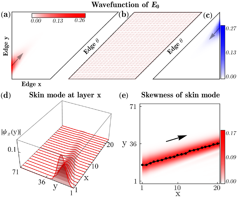
Figure 1:  The spatial distribution of wavefunction with energy $E_{0}{=}0.86{-}0.81i$ is shown under (a) trapezoid, (b) parallelogram, and (c) triangle geometries. The edge-$\theta$ is oriented along $\theta=\pi/4$, and the system size in (a) is $L_{y}{=}71$, $L_{x}{=}41$. The corresponding colorbars represent $|\psi_{E_{0}}(\bm{r})|$. (d) The wavefunction components within the first 20 $x$-layers near the edge-$y$ in (a). (e) The maximum points for each $x$-layer are selected (the black dots) and compared with the renormalized wavefunction (the red trajectory), which reveals a characteristic direction (the black arrow) of the skin mode, termed skewness. The Hamiltonian parameters in Eq.(1) are set to $t{=}2,\gamma{=}1$.

Model with edge-skin modes.— We start with an example having skin modes localized on edges. The Bloch Hamiltonian is given by:

$$h(\bm{k})=2t\cos{(k_{x}+k_{y})}-2i\gamma(1-\cos{k_{x}}),$$ (1)

where $\gamma$ introduces non-Hermiticity. We examine a typical wavefunction with energy $E_{0}$, denoted as $\psi_{E_{0}}(\bm{r})$, and show its spatial distribution for different open-boundary geometries in Fig. 1(a)(b)(c). The wavefunction exhibits geometry-dependent localization; it localizes on edge $y$ under geometries shown in Fig. 1(a)(c) but appears as a bulk mode under the geometry in Fig. 1(b).

Most importantly, despite the different open-boundary geometries, the skin mode always exhibits a stable decay behavior near the edge-$y$. Specifically, for the skin mode of $E_{0}$, we observe a decay direction extending from the edge-$y$ into bulk, as indicated by the black arrows in Fig. 1(a)(c). For enhanced clarity, we extract the wavefunction components at the first-20 $x$-layers in Fig. 1(a) and plot them in Fig. 1(d). These components decay and shift with increasing $x$-layer. In Fig. 1(e), we select the maximum point of the wavefunction in each $x$-layer (the black dots), and compare it with the wavefunction renormalized in each $x$-layer (the red trajectory). They show a distinct direction indicated by the black arrow, which we term the skewness of the skin mode near edge-$y$.

From the above numerical observations, we can pose two central questions of “where” and “how” regarding the description of edge-skin modes: (i) Is there a guiding principle to determine where (on which edge) skin modes localize ? Alternatively, for a given energy $E_{0}$, can we identify the OBC geometry where the corresponding wavefunction appears as a bulk mode? (ii) How does the skin mode decay from the localized edge to bulk? Can we determine the skewness of a generic skin mode analytically? Next, we establish an edge theory including two sections to address these questions, respectively.

Edge Theory I: bulk projection criterion for edge-skin mode.— We define a set of Fermi points $\bm{k}_{i}$ of energy $E_{0}$ in the Brillouin zone (BZ)  that satisfy $\det[h(\bm{k}_{i})-E_{0}]=0$. Each Fermi point can be assigned a topological charge Yang et al. (2021); Sup . When projecting these Fermi points onto a specific edge, say edge $y$, one can define the corresponding projective spectral winding number along the normal direction of the edge as:

$$w(E_{0},k_{y})=\frac{1}{2\pi}\int_{-\pi}^{\pi}dk_{x}\,\partial_{k_{x}}\mathrm{arg}\,\mathrm{det}[h(k_{x},k_{y})-E_{0}].$$ (2)

As illustrated in Fig. 2(a), $w(E_{0},k_{y})$ is nonzero for a range of $k_{y}$, indicated by the colored region. We thus term the edge-$y$ as nonzero-projection edge. In contrast, for edge-$x$ and edge-$\theta$, $w(E_{0},k_{x})$ and $w(E_{0},k_{\theta})$ are always zero. These edges are thereby denoted as zero-projection edges. Now we state the bulk projection criterion for the wavefunction with energy $E_{0}$: The wavefunction does not exhibit localization on open-boundary geometries composed of zero-projection edges, while it localizes at the nonzero-projection edge on the corresponding OBC geometries. This bulk projection criterion explains the geometry-dependent localization as shown in Fig. 1(a)(b)(c).

Note that the bulk Hamiltonian $h(\bm{k})$ in Eq.(1) respects inversion (or reciprocity) symmetry, which imposes the projective spectral winding in Eq.(2) further restrictions. As shown in Fig. 2(a), despite $w(E_{0},k_{y})$ being nonzero over a range of $k_{y}$, the inversion symmetry leads to a relation $w(E_{0},k_{y})=-w(E_{0},-k_{y})$, where red and blue colored region corresponds to the positive and negative projective winding numbers. This ultimately enforces the total spectral winding to be zero, indicated as $\nu_{y}(E_{0})=\int_{-\pi}^{\pi}dk_{y}w(E_{0},k_{y})=0$. In fact, this symmetry demands zero total spectral winding along every direction, mathematically expressed as $\forall\theta_{i},\,\nu_{\theta_{i}}(E_{0})=0$. Our paper focuses on cases that satisfy this condition of zero total spectral winding Sup .

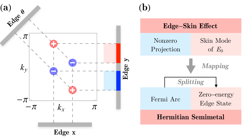
Figure 2:  (a) The Fermi points in the BZ for energy $E_{0}{=}0.86{-}0.81i$ and their projections onto specific edges. (b) The mapping from non-Hermitian edge-skin effect to Hermitian semimetal.

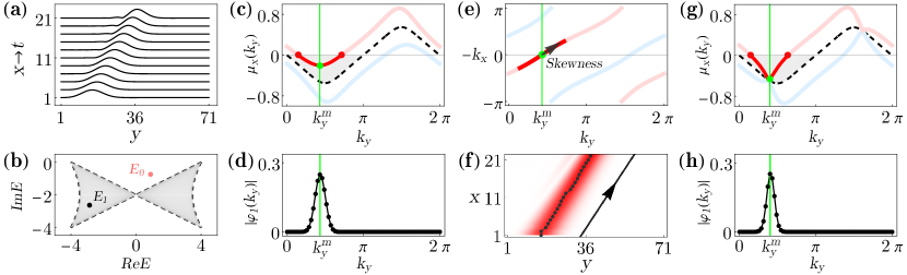
Figure 3:  The skewness of skin mode under a square geometry of system size $L_{x}=L_{y}=71$, with Hamiltonian parameters $t=2,\gamma=1$. (a) illustrates the mode components in the first 20 $x$-layers, which have been renormalized in each layer. (b) The OBC spectrum can be categorized into two regions: those outside and inside the gray region, respectively represented by $E_{0}{=}0.877{-}0.751i$ and $E_{1}{=}{-}2.867{-}2.656i$. (c)-(f) gives the skewness of the skin mode with energy $E_{0}$. (c) The solutions $\mu_{x,1}(k_{y})$ (the blue line), $\mu_{x,2}(k_{y})$ (the red line), and cylinder-geometry GBZ $\tilde{\mu}_{x}(k_{y})$ (the black-dashed line). The gray region represents the range between cylinder-geometry GBZ and BZ ($\mu_{x}(k_{y})\equiv 0$). The minimum in this range (the green dot) determines the maximum value of Fourier components of edge-layer mode components shown in (d). Correspondingly, (e) indicates the skewness as the tangential direction of $-k_{x,2}(k_{y})$ at $k_{y}^{m}$, denoted by the black arrow. (f) compares the analytical results of skewness (the black-solid arrow) with the numerical results (the black dots similar to Fig. 1(e)). (g)(h) correspond to the case of energy $E_{1}$.

To understand this bulk projection criterion, we map the non-Hermitian Hamiltonian $H_{\text{OBC}}$ to a Hermitian chiral semimetal Bernevig (2013),

$$\tilde{H}_{\text{OBC}}(E_{0})=\begin{pmatrix}0&H_{\text{OBC}}-E_{0}\\ H_{\text{OBC}}^{\dagger}-E_{0}^{*}&0\end{pmatrix},$$ (3)

with the same open-boundary geometry. Under this mapping, the Fermi points in $h(\bm{k})$ map into band crossings, e.g., Dirac points, and the nonzero-projection regions correspond to Fermi arcs in the corresponding semimetal Sup , as illustrated in Fig. 2(b). Most importantly, through this exact mapping, the edge-skin mode with energy $E_{0}$ corresponds to the zero-energy edge states of the Hermitian semimetal with fully OBCs, due to $\det[\tilde{H}_{\text{OBC}}(E_{0})]=|\det[H_{\text{OBC}}-E_{0}]|^{2}=0$. Here, the zero-energy edge states arise from the splitting of Fermi-arc states caused by fully OBCs (Fig. 2(b)). The mapping conveys dual implications Sup : (i) the projection criterion essentially inherits from the bulk-boundary correspondence in the corresponding Hermitian semimetal; (ii) Conversely, the exact zero-energy edge states in Hermitian semimetals with fully OBC geometry, a topic largely overlooked despite extensive research on Fermi-arc states , share the same spatial distribution and localization characteristics as edge-skin modes, such as geometry-dependent localization and skewness (Fig. 1).

Edge theory II: skewness of edge-skin mode.— To understand the skewness near the edge-$y$ (Fig. 1(e)), we treat the layer $x$ as time $t$, namely $(x,y)\rightarrow(t,y)$. From this perspective, mode components at different $x$-layers are mapped into a space-time dynamics. The near-edge distribution of skin mode, e.g., the first 20 $x$-layers (Fig.1(d)), corresponds to a finite-time wavepacket dynamics in the $y$ direction. When we renormalize the wavepacket at each time (Fig. 3(a)), it becomes clear that the wavepacket propagates with a velocity. In this sense, the skewness is mapped into the wavepacket group velocity. In the finite-time dynamics, the wavepacket has not yet encountered the boundaries in the $y$ direction, therefore, the velocity (or skewness) should be captured by the Hamiltonian with PBC in $y$ Mao et al. (2021) and OBC in $x$ direction, effectively being in a cylinder geometry.

We present our key results of skewness using the example in Eq.(1). After generalizing momentum $k_{x}$ into complex value $k_{x}{\rightarrow}k_{x}{-}i\mu_{x}$ and taking the substitution $\beta_{x}\coloneqq e^{ik_{x}+\mu_{x}}$, the corresponding non-Bloch Hamiltonian with real-valued edge momenta $k_{y}$ can be expressed as

$$\mathcal{H}(\beta_{x},k_{y})=c_{+}(k_{y})\beta_{x}+c_{-}(k_{y})\beta_{x}^{-1}-2i\gamma,$$ (4)

where $c_{\pm}(k_{y})=te^{\pm ik_{y}}+i\gamma$. The solution of $\log|\beta_{x}(k_{y})|\equiv\mu_{x}(k_{y})$ can be obtained by solving $\det[\mathcal{H}(\beta_{x},k_{y})-E]=0$. Based on the non-Bloch theorem, the GBZ for the cylinder-geometry Hamiltonian Sup is represented by

$$\tilde{\mu}_{x}(k_{y})\equiv\mu_{x,1}(k_{y},E)=\mu_{x,2}(k_{y},E),$$ (5)

which is satisfied only when $E$ is in the cylinder-geometry spectrum (denoted by $\sigma_{\text{cyl}}$, the gray region in Fig. 3(b)). Given that the OBC spectrum is generally inconsistent with cylinder-geometry spectrum, the OBC eigenvalues can be sorted into two sections: $E\notin\sigma_{\text{cyl}}$ and $E\in\sigma_{\text{cyl}}$, as illustrated in Fig. 3(b).

Under the space-time mapping, $x$ serves as the temporal parameter $t$, therefore, its conjugate quantity, $-k_{x}$ and $\mu_{x}$, can be considered as the real and imaginary parts of ‘complex energy band’. In this sense, $v(k_{y})=-\partial_{k_{y}}k_{x}(k_{y})$ represents the group velocity of the wavepacket, and $a(k_{y})=\partial_{k_{y}}\mu_{x}(k_{y})$ has the meaning of acceleration. As such, the velocity (or skewness) near the edge is governed by the edge momentum center, i.e., the momentum center of the mode components at edge layer $x=1$. Now we state the first key finding of skewness for the skin mode with energy $E_{0}$: in the large-size limit, the edge momentum center always converges to the minimum point $k_{y}^{m}$ where $\mu_{x}(k_{y}^{m},E_{0})$ reaches its minimum in the range of $\tilde{\mu}_{x}(k_{y})<\mu_{x}(k_{y},E_{0})<0$.

Here we provide a straightforward proof for this statement, with more details available in Sup . We begin with the mode components at layer $x_{0}$ away from the edge, which can be generally decomposed as $\psi_{x_{0}}(y)=\int_{-\pi}^{\pi}dk_{y}\,\varphi_{x_{0}}(k_{y})\,e^{ik_{y}y}$. $\varphi_{x_{0}}(k_{y})$ represents the Fourier components at layer $x_{0}$. The mode components amplify from the bulk to the edge (along the $-x$ direction), the amplification rate for each $k_{y}$ can be determined by the propagator

$$|\mathcal{G}_{E_{0}}(-x,k_{y})|=\left|\oint_{C_{\beta_{x}}}\frac{d\beta_{x}}{\beta_{x}}\frac{\beta_{x}^{-x}}{E_{0}^{+}-\mathcal{H}(\beta_{x},k_{y})}\right|\propto e^{-\mu_{x}(k_{y})x},$$

where the integral contour $C_{\beta_{x}}$ is the cylinder-geometry GBZ and $E_{0}$ is the OBC eigenvalue of the skin mode. The integral value is finally determined by the poles $\mu_{x}$ within the range between GBZ ($\tilde{\mu}_{x}(k_{y})$) and BZ ($\mu_{x}(k_{y})\equiv 0$), represented by the red opaque arc within the gray region in Fig. 3(c). Therefore, the minimum of $\mu_{x}(k_{y})$ in this range, denoted by the green dot in Fig. 3(c), leads to the maximal amplification rate and determines the momentum center at the edge layer $x=1$, as shown in Fig. 3(d).

In the case of skin mode with energy $E_{0}\notin\sigma_{\text{cyl}}$ (Fig. 3(b)), there are two gapped ‘energy bands’ with different imaginary parts $\mu_{x,1}(k_{y})<\tilde{\mu}_{x}(k_{y})<\mu_{x,2}(k_{y})<0$ (Fig. 3(c)). The ‘gap’ here specifically means that $\mu_{x,i}(k_{y})$ does not intersect with $\tilde{\mu}_{x}(k_{y})$ (the black-dashed line in Fig. 3(c)). Based on our first finding, the edge momentum center always converges to the minimum point of $\mu_{x,2}(k_{y})$, denoted by $k_{y}^{m}$ in Fig. 3(c). In the case of $E_{0}\notin\sigma_{\text{cyl}}$, it further satisfies:

$$\partial_{k_{y}}\mu_{x,2}(k_{y}^{m})=0.$$ (6)

It means that the initial wavepacket has zero acceleration, $a(k_{y}^{m})=\partial_{k_{y}}\mu_{x,2}(k_{y}^{m})=0$, and thus will propagate with a constant velocity. This constant velocity, exactly the skewness, is given by:

$$s_{\text{edge{-}y}}(E_{0})=-\partial_{k_{y}}k_{x,2}(k_{y}^{m}),$$ (7)

which is denoted by the black arrow in Fig. 3(e). As an example, we select the skin mode with energy $E_{0}{=}0.877{-}0.751i$. From Eq.(6) and Eq.(7), the corresponding skewness is analytically calculated as $s_{\text{edge{-}y}}(E_{0}){=}1.113$. In Fig. 3(f), we plot the analytical result $y(x)=s_{\text{edge{-}y}}(E_{0})\,x+y_{0}$ as the black-solid arrow, and compare it with the numerical results (the black dots similar to Fig. 1(e)), which shows perfect agreement. This second key finding indicates that the skewness of the skin mode is only determined by the non-Bloch Hamiltonian with real-valued edge momenta without requiring any boundary details, thus serving as an intrinsic quantity of the skin mode.

For the case of energy $E_{1}\in\sigma_{\text{cyl}}$, the corresponding solutions $\mu_{x,i}(k_{y})$ intersect with $\tilde{\mu}_{x}(k_{y})$ (Fig. 3(g)). The edge-layer momentum distribution is depicted in Fig. 3(f). However, in this case the edge momentum center may not satisfy Eq.(6). Therefore, the skewness of skin mode will bend when away from the edge Sup . These findings on skewness can be directly generalized and applicable to more generic models with long-range hopping, as detailed in Sup .

Anomalous spectral sensitivity in edge-skin effect and emergence of skewness.— The reciprocity or inversion symmetry in the bulk Hamiltonian described by Eq.(4) ensures that the characteristic equation satisfies

$$\begin{split}f_{E}(k_{x},\mu_{x},k_{y})=f_{E}(-k_{x},-\mu_{x},-k_{y})=0,\end{split}$$ (8)

which we term fragile reciprocity. Note that fragile reciprocity is readily violated by factors such as onsite disorders or open boundaries that break translation in $y$ direction, hence the name of ‘fragile’. With this symmetry, the non-Bloch Hamiltonian in Eq.(4) has two key features: (i) the $k_{y}$ components are decoupled with each other, and (ii) the doubly degenerate non-Bloch waves with opposite $k_{y}$ exhibit opposite localization in the $x$ direction. When the translation in $y$ direction is broken, these non-Bloch waves can be coupled to form eigen wavefunction. It is reasonable to expect that the skewness in the wavefunction can be observed when the fragile reciprocity is broken. Meanwhile, a remarkable sensitivity of the spectrum is also anticipated, due to the splitting of the degeneracy in non-Bloch waves.

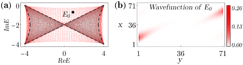
Figure 4:  (a) When we introduce the weak random disorders with strength $W{=}0.1$ in Eq.(9) to the cylinder-geometry Hamiltonian, the spectrum remarkably shifts from the region bounded by the black-dashed line to the red dots. (b) shows the spatial distribution of the wavefunction with energy $E_{0}{=}0.89{-}0.7i$ selected in (a).

Numerically, to break the fragile reciprocity, we introduce a line of weak onsite disorders into the Hamiltonian Eq.(4) with PBC in $y$ and OBC in $x$ direction,

$$\hat{V}=\sum\nolimits_{x}V_{x}\,\hat{c}^{\dagger}_{x,y_{0}}\hat{c}_{x,y_{0}};\,\,\,\,V_{x}\in[0,W],$$ (9)

where $V_{x}$ represents the strength of onsite potential at the lattice site $(x,y_{0})$ with fixed $y=y_{0}$ and is randomly distributed in the range $[0,W]$. As shown in Fig. 4(a), the spectrum is remarkably shifted from the gray region, enclosed by the black-dashed boundary, to the red dots upon introducing weak onsite disturbances with $W=0.1$. Accordingly, the spatial distribution of wavefunction with energy $E_{0}$ selected in Fig. 4(a) shows the skewness, similar to that in Fig. 1.

We emphasize that in the case of the corner-skin effect or 1D non-Hermitian skin effect, the weak onsite disorders can be typically treated as perturbations to the spectrum Fang et al. (2023); see more examples in Sup . Therefore, this anomalous spectral sensitivity and emergence of skewness are unique to edge-skin effect and crucially distinguishes from the corner-skin effect.

Conclusion.— In summary, we establish an effective edge theory to describe the higher-dimensional edge-skin modes. For a generic edge-skin mode, the edge theory includes two parts: (i) We propose a bulk projection criterion to diagnose the localized edge; (ii) We find an intrinsic decay direction of the skin mode, termed skewness, which can be accurately captured by the non-Bloch bulk Hamiltonian with real-valued edge momenta without requiring any boundary details. Lastly, unique to the edge-skin effect, we reveal the anomalous sensitivity of the spectrum to perturbations that break fragile reciprocity, accompanied by the emergence of the skewness in the corresponding wavefunctions.

Acknowledgments.— This work was supported in part by the Office of Naval Research MURI N00014-20-1-2479 (K.Z. and K.S.), the Gordon and Betty Moore Foundation Grant No. N031710 (K.S.), and the Office Navy Research Award N00014-21-1-2770 (K.S.). Z.Y. acknowledges funding supported by the National Science Foundation of China (Grant No. NSFC-12322405, -12104450) and the fellowship of China National Postdoctoral Program for Innovative Talents (Grant No. BX2021300).

Supplemental Material for “Edge theory of the non-Hermitian skin modes in higher dimensions”

S-1 Edge Theory I: bulk projection criterion and the mapping to Hermitian semimetals

In this section, firstly, we classify the higher-dimensional non-Hermitian skin modes into two classes, namely corner-skin and edge-skin modes, according to the total spectral winding number. Secondly, we discuss the symmetries that can enforce the edge-skin effect. Lastly, we elaborate on the mapping between the non-Hermitian edge-skin effect and Hermitian semimetals.

S-1.1 The classification of higher-dimensional skin effect

Here we classify the (non-Hermitian) skin modes in two-dimensional systems according to the total spectral winding number. For a given Bloch Hamiltonian $h(k_{x},k_{y})$, we first define the spectral winding number in the $x$ direction with fixed $k_{y}$

$$w(E_{0},k_{y})=\frac{1}{2\pi}\int_{-\pi}^{\pi}dk_{x}\,\partial_{k_{x}}\arg{\det{[h(k_{x},k_{y})-E_{0}]}},$$ (S1)

where $E_{0}$ represents a generic OBC eigenvalue, serving as a reference energy here. Note that the OBC continuum spectrum is always covered by the PBC spectrum. Therefore, $E_{0}$ is included in the spectrum of $h(k_{x},k_{y})$. Assuming that there are some $(k_{x},k_{y})$ points such that $\det{[h(k_{x},k_{y})-E_{0}]}=0$, these points are termed Fermi points in the main text. When calculating the spectral winding number defined in Eq.(S1), we need to avoid these Fermi points such that the spectral winding number is well-defined. For a given energy $E_{0}$ and fixed $k_{y}$, we now have the corresponding spectral winding number $w(E_{0},k_{y})$.

Next, we define the total spectral winding number for the $y$ direction as the integral of $w(E_{0},k_{y})$ over $k_{y}$, that is,

$$\nu_{y}(E_{0})=\frac{1}{2\pi}\int_{-\pi}^{\pi}dk_{y}\,w(E_{0},k_{y}),$$ (S2)

of which the value depends on the reference energy $E_{0}$ and direction $y$. Based on the above definition, we have the total spectral winding for an arbitrary direction $\theta$, mathematically expressed as,

$$\nu_{\theta}(E_{0})=\frac{1}{2\pi}\int_{-\pi}^{\pi}dk_{\theta}\,w(E_{0},k_{\theta})=\frac{1}{(2\pi)^{2}}\int_{-\pi}^{\pi}dk_{\theta}\,\int_{-\pi}^{\pi}dk_{\bot}\partial_{k_{\bot}}\arg{\det{[h(k_{\bot},k_{\theta})-E_{0}]}},$$ (S3)

where $k_{\bot}$ represents the momenta along the normal direction of $\theta$. Mathematically, there are two mutually exclusive and complete cases:

$$\begin{split}&(\mathrm{i})\,\,\,\exists\,\theta;\,\nu_{\theta}(E_{0})\neq 0;\\ &(\mathrm{ii})\,\,\forall\,\theta;\,\nu_{\theta}(E_{0})=0.\end{split}$$ (S4)

These two cases correspond to two classes of skin modes: the corner-skin modes in case (i) and the edge-skin modes in case (ii). It is important to note that case (ii) can be enforced by symmetries in the bulk Hamiltonian, which we will discuss later. In most generic cases, the Hamiltonian without any specific symmetry corresponds to case (i), thereby exhibiting the corner-skin effect.

In case (i), the skin mode prefers to localize at a specific corner of a polygon, such as a square geometry, thus termed corner-skin mode. As an illustration, consider a skin mode with energy $E_{0}$ in a square geometry under case (i), generally, $\nu_{x}(E_{0})\neq 0$ and $\nu_{y}(E_{0})\neq 0$. The nonzero total spectral winding implies $w(E_{0},k_{x})\neq 0$ for some $k_{x}$ and $w(E_{0},k_{y})\neq 0$ for some $k_{y}$ as defined in Eq.(S1). We generalize $k_{x}$ and $k_{y}$ into complex value $k_{x}-i\mu_{x}$ and $k_{y}-i\mu_{y}$, respectively. According to the recently established amoeba formula Wang et al. (2022); Hu (2023), one can always find suitable $\mu_{x}\neq 0$ and $\mu_{y}\neq 0$ such that the total spectral winding

$$\begin{split}&\tilde{\nu}_{x}(E_{0})=\frac{1}{(2\pi)}\int_{-\pi}^{\pi}dk_{x}\,w(E_{0},k_{x}-i\mu_{x})=0;\\ &\tilde{\nu}_{y}(E_{0})=\frac{1}{(2\pi)}\int_{-\pi}^{\pi}dk_{y}\,w(E_{0},k_{y}-i\mu_{y})=0.\end{split}$$

The nonzero $\mu_{x}$ and $\mu_{y}$ give us the effective localization length in $x$ and $y$ directions, respectively. It ultimately means that the skin mode will be localized at the corner of a square lattice.

In fact, the two-dimensional corner-skin effect is very similar to the one-dimensional skin effect. In one dimension, case (i) given by Eq.(S4) reduces to a nonzero Bloch spectral winding number, namely, $\nu(E_{0})=\frac{1}{(2\pi)}\int_{-\pi}^{\pi}dk\,\partial_{k}\mathrm{arg}\,\mathrm{det}[h(k)-E_{0}]\neq 0$. It was known that in one dimension, nonzero Bloch spectral winding number regarding the reference energy $E_{0}$ means that the OBC wavefunction of $E_{0}$ appears as a skin mode under OBCs Zhang et al. (2020); Okuma et al. (2020). Similarly, one can extend $k$ into complex value $k-i\mu$ such that the spectral winding number vanishes, that is, $\tilde{\nu}(E_{0})=\frac{1}{(2\pi)}\int_{-\pi}^{\pi}dk\,\partial_{k}\mathrm{arg}\,\mathrm{det}[h(k-i\mu)-E_{0}]=0$. Finally, nonzero $\mu$ characterizes the localization length of the skin mode with energy $E_{0}$.

Obviously, the above argument fails for case (ii), since the total spectral winding is already zero. It implies that the localization feature in case (ii) is essentially different from the corner-skin effect in case (i). In case (ii), the zero total spectral winding means that there is no net non-reciprocity along any spatial direction. From extensive numerical observations, the skin modes in case (ii) are generally localized on the edges of a polygon, thus termed edge-skin modes.

However, the stable edge-localization of skin modes is quite confusing, since the non-Bloch wave components always have exponential envelopes, formally expressed as $\beta_{x}^{x}\beta_{y}^{y}=e^{i(k_{x}x+k_{y}y)}e^{\mu_{x}x+\mu_{y}y}$, which are typically localized at corners of a polygon, such as a square geometry. This implies that it is sufficiently difficult to construct an edge-localized skin mode using the exponentially localized non-Bloch waves, characterize by the form $\beta_{x}^{x}\beta_{y}^{y}$. Under this background, to find a concise and effective edge description to address this puzzle is urgently needed. As discussed in the later section S-1.3, we establish an exact mapping from the non-Hermitian edge-skin modes to the zero-energy edge states of a Hermitian semimetals, which helps us to understand why the skin modes prefer to localize on the edges.

S-1.2 Symmetry in the edge-skin effect

Here we show that the inversion symmetry or reciprocity in the bulk Hamiltonian $h(\bm{k})$ can guarantee case (ii) in Eq.(S4), thereby enforcing the Hamiltonian to manifest the edge-skin effect. The Hamiltonian satisfying these two symmetries can be expressed as:

$$\begin{split}&\mathcal{U}_{I}h(\bm{k})\mathcal{U}_{I}^{\dagger}=h(-\bm{k});\\ &\mathcal{U}_{T}h^{T}(\bm{k})\mathcal{U}_{T}^{\dagger}=h(-\bm{k}),\end{split}$$ (S5)

for inversion and reciprocity, respectively. Here, $\mathcal{U}_{I}$ or $\mathcal{U}_{T}$ represents the unitary matrix of the corresponding symmetry. With these symmetries, the spectral winding number defined in Eq.(S1) satisfies:

$$\begin{split}w(E_{0},k_{y})&=\frac{1}{2\pi}\int_{-\pi}^{\pi}dk_{x}\,\partial_{k_{x}}\arg{\det{[h(k_{x},k_{y})-E_{0}]}}=\frac{1}{2\pi}\int_{-\pi}^{\pi}dk_{x}\,\partial_{-k_{x}}\arg{\det{[h(-k_{x},k_{y})-E_{0}]}}\\ &=-\frac{1}{2\pi}\int_{-\pi}^{\pi}dk_{x}\,\partial_{k_{x}}\arg{\det{[h(k_{x},-k_{y})-E_{0}]}}=-w(E_{0},-k_{y}),\end{split}$$ (S6)

where the third equality holds due to the symmetries in the bulk Hamiltonian, as shown in Eq. (S5). Therefore, with these symmetries, the total spectral winding number over $k_{y}$ must be zero, expressed as:

$$\nu_{y}(E_{0})=\frac{1}{2\pi}\int_{-\pi}^{\pi}dk_{y}w(E_{0},k_{y})=0.$$ (S7)

In fact, the symmetry necessitates zero total spectral winding along every direction, namely,

$$\forall\theta;\,\,\,\,\nu_{\theta}(E_{0})=0,$$ (S8)

which corresponds to case (ii) defined in Eq.(S4). In conclusion, either inversion or reciprocity enforces the Hamiltonian to exhibit the edge-skin effect. One example is the Hamiltonian in Eq.(1) of the main text. The single-band model Hamiltonian respects inversion (or reciprocity) symmetry, therefore, it exhibits edge-skin effect with fully OBCs.

Notably, in one dimension, reciprocity or inversion symmetry requires the spectral winding number to vanish and hence forbids the non-Hermitian skin effect Kawabata et al. (2020); Yi and Yang (2020). In sharp contrast, in two and higher dimensions, the edge-skin effect can coexist with these symmetries. Therefore, edge-skin effect is unique to higher dimensions.

When we consider the mirror symmetry and combined mirror-reciprocity, expressed as $\mathcal{M}_{\theta}h(k_{\bot},k_{\theta})\mathcal{M}_{\theta}^{\dagger}=h(k_{\bot},-k_{\theta})$ and $\mathcal{M}_{\theta}h^{T}(k_{\bot},k_{\theta})\mathcal{M}_{\theta}^{\dagger}=h(-k_{\bot},k_{\theta})$, respectively, there are three cases. (i) mirror symmetry in both directions, (ii) mirror symmetry and combined mirror-reciprocity, and (iii) mirror-reciprocity in both directions. When the Hamiltonian respects one of these three symmetries, inversion or reciprocity also holds, and Eq.(S8) must be satisfied, thereby guaranteeing the edge-skin effect.

S-1.3 The bulk projection criterion and mapping to Hermitian semimetals

In this subsection, we elaborate on the bulk projection criterion and its mapping to Hermitian semimetals by presenting a numerical example. Specifically, for a given edge-skin mode with energy $E_{0}$, the corresponding bulk projection criterion determines the localized edges. On the one hand, the exact mapping helps to understand why the bulk projection criterion works well. On the other hand, through this exact mapping, the localization features of the edge-skin mode, such as geometry-dependent localization and the skewness (as discussed in Sec. S-2), can be directly applied to the zero-energy edge states in the Hermitian semimetal with fully OBCs.

Notably, although the Fermi-arc states in semimetals under semi-infinite boundary conditions are frequently investigated Bernevig (2013), the exact zero-energy edge states under fully OBCs are often overlooked. This expands the scope of our edge theory.

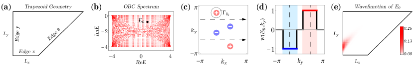
Figure S1: The illustration for the bulk-edge correspondence in the edge-skin effect. (a) The lattice geometry is depicted with a trapezoid of size $L_{x}=45$, $L_{y}=71$, and the edge $\theta$ oriented in the direction of $\theta=\pi/4$. (b) The eigenvalues of the Hamiltonian in Eq.(S9) under the trapezoid geometry are depicted by the red dots. A specific OBC eigenvalue, $E_{0}=0.866-0.814i$, is indicated by the black dot. The Fermi points of $E_{0}$ are shown in (c), where the sign ‘$\pm$’ represents the topological charge of each Fermi point. We select two paths with fixed $k_{y}$, indicated by the black arrows, the corresponding spectral winding numbers are shown in (d). $w(E_{0},k_{y})=\pm 1$ for a range of $k_{y}$. According to the projection criterion, the skin mode with energy $E_{0}$ is localized on the edge $y$, as illustrated in (e). The system parameters are set to $t=2,\gamma=1$.

S-1.3.1 The bulk projection criterion

We use the example of edge-skin effect discussed in the main text. The Bloch Hamiltonian is given by

$$h(\bm{k})=2t\cos{(k_{x}+k_{y})}-2i\gamma(1-\cos{k_{x}}),$$ (S9)

with parameters $t=2,\gamma=1$ set for our discussion. Under the open boundary condition with a trapezoid geometry, as illustrated in Fig. S1(a), the OBC eigenvalues can be evaluated and represented by red dots in Fig. S1(b). Here, the system size is $L_{y}=71,L_{x}=41$. For a generic OBC eigenvalue $E_{0}=0.866-0.814i$, indicated by the black dot in Fig. S1(b), we have a set of Fermi points $\bm{k}_{i}$ that satisfy $\det{[h(\bm{k}_{i})-E_{0}]}=0$, as shown in Fig. S1(c). For each Fermi point, we can assign a topological charge that is defined as:

$$C_{E_{0}}(\bm{k}_{i})=\frac{1}{2\pi}\oint_{\Gamma_{\bm{k}_{i}}}d\bm{k}\,\partial_{\bm{k}}\arg{\det[h(\bm{k}_{i})-E_{0}]},$$ (S10)

where $\Gamma_{\bm{k}_{i}}$ represents the integral contour encircling Fermi point $\bm{k}_{i}$ counterclockwise. In such a way, the topological charges of these four Fermi points of $E_{0}$ can be obtained and indicated by the ‘$\pm$’ signs corresponding to $C_{E_{0}}(\bm{k}_{i})=\pm 1$. As shown in Fig. 2(a) of the main text, these four Fermi points have zero projection onto edge-$x$ and edge-$\theta$, while have nonzero projection onto edge-$y$. It means that $w(E_{0},k_{y})\neq 0$ defined in Eq.(S1) for a range of $k_{y}$, as depicted in Fig. S1(d). Meanwhile, due to the inversion symmetry in the Hamiltonian Eq.(S9), the spectral winding satisfies $w(E_{0},k_{y})=-w(E_{0},-k_{y})$, as shown in Fig. S1(d), which ensures the zero total spectral winding number (Eq.(S8)).

According to the bulk projection criterion, the wavefunction of $E_{0}$ does not exhibit localization on the open-boundary geometry comprising edge-$x$ and edge-$\theta$ (as shown in Fig.1(b) in the main text), whereas it localizes at edge-$y$ in the trapezoidal geometry, as depicted in Fig. S1(e). It is important to note that with different OBC eigenvalues $E_{0}$, the distribution of Fermi points in the BZ will be different. Consequently, the projection of Fermi points on different edges changes, leading to distinct localization behaviors of the corresponding wavefunction.

S-1.3.2 The mapping to a Hermitian semimetal

Here we utilize an exact mapping that maps the non-Hermitian Hamiltonian with the edge-skin effect to a Hermitian chiral semimetal, which helps to better understand the bulk projection criterion.

Under this mapping Gong et al. (2018); Kawabata et al. (2019), the non-Hermitian Bloch Hamiltonian in Eq.(S9) is mapped into

$$\tilde{h}_{E_{0}}(\bm{k})=\begin{pmatrix}0&h(\bm{k})-E_{0}\\ h^{\dagger}(\bm{k})-E_{0}^{\ast}&0\end{pmatrix}=(2t\cos{(k_{x}+k_{y})}-E_{0}^{r})\,\sigma_{x}+(2\gamma\,(1-\cos{k_{x}})+E_{0}^{i})\,\sigma_{y},$$ (S11)

where $E_{0}^{r},E_{0}^{i}$ represent the real and imaginary parts of the complex $E_{0}$, respectively, and $\sigma_{x}$ and $\sigma_{y}$ are the Pauli matrices. It should be noted that the Hermitian Hamiltonian always respects an additional chiral symmetry,

$$\sigma_{z}\tilde{h}_{E_{0}}(\bm{k})\sigma_{z}=-\tilde{h}_{E_{0}}(\bm{k}).$$

Since $\det[h(\bm{k})-E_{0}]=0$ at Fermi points, as depicted in Fig. S2(b), the mapped Hermitian Hamiltonian satisfies

$$\det[\tilde{h}_{E_{0}}(\bm{k})]=\det[h(\bm{k})-E_{0}]*\det[h^{\dagger}(\bm{k})-E_{0}^{\ast}]=0$$

at the Dirac points, as shown in Fig. S2(c). It means that the Hermitian Hamiltonian $\tilde{h}_{E_{0}}(\bm{k})$ is always gapless at zero energy and has the chiral symmetry. Therefore, the mapped Hermitian Hamiltonian is always a chiral semimetal Bernevig (2013).

Through this mapping, the Fermi points in the non-Hermitian Hamiltonian map to Dirac points in the Hermitian chiral semimetal. The nonzero projection region corresponds to the Fermi-arc region in $k_{y}$, as illustrated in Fig. S2(b)(c).

Now we show that the non-Hermitian edge-skin mode with $E_{0}$ can be mapped into the zero-energy edge states in the Hermitian semimetal. The mapping can be formally expressed as:

$$\tilde{H}_{\text{OBC}}(E_{0})=\begin{pmatrix}0&H_{\text{OBC}}-E_{0}\\ H_{\text{OBC}}^{\dagger}-E_{0}^{*}&0\end{pmatrix},$$ (S12)

with the same open-boundary geometry, for example, the trapezoid geometry depicted in Fig. S1(a). Under the fully OBCs, the Fermi-arc states with order-$L$ ($L$ generally representing the lattice length) will split. However, there always exist the order-1 zero-energy edge states reserved, owing to $\det[\tilde{H}_{\text{OBC}}(E_{0})]=|\det[H_{\text{OBC}}-E_{0}]|^{2}=0$. Therefore, the complex energy $E_{0}$ in the non-Hermitian Hamiltonian, as indicated by the red dot in Fig. S2(d) is mapped into the zero-energy edge states, denoted by the blue dots in Fig. S2(e).

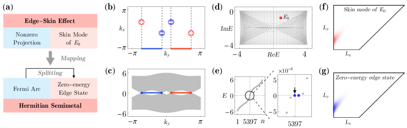
Figure S2: (a) The mapping from the non-Hermitian edge-skin effect to a Hermitian semimetal is detailed. Specifically, the Fermi points that have nonzero projections on the edge $y$ in (b) are mapped to Dirac points featuring connected Fermi-arcs in (c). In (c), the energy bands are calculated using the Hamiltonian Eq.(S11) with $E_{0}=0.866-0.814i$, under PBC in the $y$ and OBC in the $x$ direction, and with $L_{x}=61$. The OBC eigenvalue $E_{0}$ (d) in the non-Hermitian Hamiltonian Eq.(S9) is mapped to two exact zero energies (e) in the Hermitian semimetal Eq.(S11). In (e), the horizontal axis $n$ represents the $n$-th eigenvalue ordered by their magnitudes. Correspondingly, the skin mode of $E_{0}$ (f) is mapped into the zero-energy edge state (g). They show the same spatial distribution under the same lattice geometry. Notably, the two zero-energy edge states remain after the splitting of Fermi-arc states induced by the fully OBCs. The system parameters are set to $t=2,\gamma=1$.

For a given energy $E_{0}$ in the non-Hermitian Hamiltonian, we can define the left and right eigenvectors as follows,

$$H_{\text{OBC}}|\psi^{R}_{E_{0}}\rangle=E_{0}|\psi^{R}_{E_{0}}\rangle;\quad H_{\text{OBC}}^{\dagger}|\psi^{L}_{E_{0}}\rangle=E^{\ast}_{0}|\psi^{L}_{E_{0}}\rangle.$$ (S13)

Here the superscripts $R/L$ denote the right/left eigenvectors. The skin mode with energy $E_{0}$ refers to the right eigenvector, $\psi_{E_{0}}(\bm{r})\equiv\langle\bm{r}|\psi^{R}_{E_{0}}\rangle$. Using the mapping given by Eq.(S12), the Hermitian Hamiltonian with the same OBC geometry must have two degenerate zero-energy edge states, expressed as

$$\tilde{H}_{\text{OBC}}(E_{0})|\tilde{\psi}_{0}\rangle=\tilde{H}_{\text{OBC}}(E_{0})\begin{pmatrix}\bm{0}\\ |\psi^{R}_{E_{0}}\rangle\end{pmatrix}=0;\quad\tilde{H}_{\text{OBC}}(E_{0})|\tilde{\psi}^{\prime}_{0}\rangle=\tilde{H}_{\text{OBC}}(E_{0})\begin{pmatrix}|\psi_{E_{0}}^{L}\rangle\\ \bm{0}\end{pmatrix}=0,$$ (S14)

where $\bm{0}$ denotes the zero column vector. We emphasize that the zero-energy edge states $|\tilde{\psi}_{0}\rangle$ and $|\tilde{\psi}^{\prime}_{0}\rangle$ under OBCs arise from the splitting of Fermi-arc states, which are often overlooked in the investigation of Hermitian semimetals. There are two degrees of freedom per unit cell, we define the spatial distribution of zero-energy edge states as

$$\tilde{W}_{0}(\bm{r})=\sum_{\alpha=A,B}|\tilde{\psi}_{0,\alpha}(\bm{r})|^{2};\quad\tilde{W}^{\prime}_{0}(\bm{r})=\sum_{\alpha=A,B}|\tilde{\psi}^{\prime}_{0,\alpha}(\bm{r})|^{2}.$$ (S15)

Here $\tilde{\psi}_{0,A}(\bm{r})=0$ and $\tilde{\psi}_{0,B}(\bm{r})=\psi^{R}_{E_{0}}(\bm{r})$, $\tilde{\psi}^{\prime}_{0,A}(\bm{r})=\psi^{L}_{E_{0}}(\bm{r})$ and $\tilde{\psi}^{\prime}_{0,B}(\bm{r})=0$.

In the edge-skin effect, the reciprocity requires the Hamiltonian matrix in real space to satisfy $H^{T}=H$. It follows from Eq.(S13) that

$$(H^{\dagger}-E_{0}^{\ast})|\psi_{E_{0}}^{L}\rangle=(H^{T}-E_{0})|\psi_{E_{0}}^{L}\rangle^{\ast}=(H-E_{0})|\psi_{E_{0}}^{L}\rangle^{\ast}=0.$$

Comparing this with the eigenequation for the right eigenvector, we obtain

$$|\psi^{R}_{E_{0}}(\bm{r})|^{2}=|\psi^{L}_{E_{0}}(\bm{r})|^{2}.$$

Finally, we conclude that the two degenerate zero modes and the edge-skin mode $|\psi^{R}_{E_{0}}\rangle$ share identical spatial distributions, expressed as

$$\tilde{W}_{0}(\bm{r})=\tilde{W}^{\prime}_{0}(\bm{r})=W_{E_{0}}(\bm{r})=|\psi_{E_{0}}^{R}(\bm{r})|^{2}.$$ (S16)

As an example, we select $E_{0}=0.866-0.814i$ as denoted in Fig. S2(d). The corresponding skin mode under the trapezoid geometry (Fig. S1(a)) is plotted Fig. S2(f), with system size $L_{y}=71$ and $L_{x}=41$. Through the mapping defined in Eq.(S12), the spatial distribution of the zero-energy edge state indicated by the black arrow in Fig. S2(e) is depicted in Fig. S2(g). They show the identical spatial distribution. In conclusion, the mapping between non-Hermitian edge-skin effect and Hermitian semimetal is illustrated in Fig. S2(a).

S-2 Edge theory II: skewness of the edge-skin mode

This section focuses on the skewness of the skin mode, including two parts. Firstly, we present a detailed proof demonstrating that: For an edge-skin mode with energy $E_{0}$, the momentum center of its edge-layer component is totally determined by the non-Bloch bulk Hamiltonian with real-valued edge momenta in the large-size limit. Building on this, we can analytically determine the skewness for a given skin mode, and then extend this formula to more generic cases involving long-range hopping, verified by numerical examples.

Here we elucidate some motivations and terminologies. Consider a generic edge-skin mode with energy $E_{0}$ that is localized on edges, for example the edge-$y$ shown in Fig. S1(e). To describe how the skin mode decays from the edge into bulk, we define a characteristic decay direction in terms of the maximum point for each layer-$x$ component of the skin mode, as illustrated in Fig. 1 of the main text. We term this direction skewness.

Generally, the skin mode of $E_{0}$ could be localized on multiple edges. For each localized edge, we can define a corresponding decay direction in such a way. In this section, we demonstrate that the skewness for each localized edge is an intrinsic quantity of the skin mode. It can be solely determined by the non-Bloch bulk Hamiltonian with real-valued momenta along the localized edge in the $\theta$ direction. The non-Bloch Hamiltonian can be formally expressed as $\mathcal{H}(\beta_{\bot},k_{\theta})$.

S-2.1 The detailed proof on the momentum center of edge-layer component

S-2.1.1 The non-Bloch Hamiltonian with real-valued edge momenta

We begin with the example given by Eq.(S9). The skin mode with energy $E_{0}$, denoted as $\psi_{E_{0}}(\bm{r})$, under the square geometry is illustrated in Fig. S3(a). The system size is $L_{x}=L_{y}=71$. The layer-$x_{0}$ component of the skin mode is denoted by $\psi_{E_{0}}(x_{0},y)$. Therefore, the edge-layer components are $\psi_{E_{0}}(1,y)$ and $\psi_{E_{0}}(L_{x},y)$ for left- and right-side $y$-edges, respectively. Here, we only focus on the edge-layer component $\psi_{E_{0}}(1,y)$.

We extract the first 20 $x$-layers components near the edge layer $x=1$, indicated by the gray region surrounded by the black dashed box in Fig. S3(a), and plot them in Fig. S3(b). These components decay and their centers (the black dots in Fig. S3(b)) shifts when away from the edge. When we consider the layer $x$ as time $t$, namely $(x,y)\rightarrow(t,y)$, the near-edge components of skin mode corresponds to a finite-time wavepacket dynamics in the $y$ direction. The wavepacket decays and propagates with a velocity. By definition, the skewness is exactly mapped into the wavepacket group velocity. In the finite-time dynamics, the wavepacket has not yet encountered the boundaries in the $y$ direction, therefore, the velocity (or skewness) should be captured by the Hamiltonian with PBC in $y$ Mao et al. (2021) and OBC in $x$ direction, effectively being in a cylinder geometry.

For the Hamiltonian in Eq.(S9), we generalize momentum $k_{x}$ into complex value $k_{x}{\rightarrow}k_{x}{-}i\mu_{x}$ and taking the substitution $\beta_{x}\coloneqq e^{ik_{x}+\mu_{x}}$. The corresponding non-Bloch Hamiltonian with real-valued edge momenta $k_{y}$ can be expressed as

$$\mathcal{H}(\beta_{x},k_{y})=c_{+}(k_{y})\beta_{x}+c_{-}(k_{y})\beta_{x}^{-1}-2i\gamma,$$ (S17)

where $c_{\pm}(k_{y})=t\,e^{\pm ik_{y}}+i\gamma$ with parameters $t=2$ and $\gamma=1$. For each fixed $k_{y}$, $\mathcal{H}(\beta_{x},k_{y})$ reduces to 1D non-Bloch Hamiltonian. Using the 1D non-Bloch theorem Yao and Wang (2018); Yokomizo and Murakami (2019), the $k_{y}$-dependent generalized Brillouin zone (GBZ) can be expressed as

$$|\beta_{x,1}(E,k_{y})|=|\beta_{x,2}(E,k_{y})|,$$ (S18)

where $\beta_{x,i}(E,k_{y})$ represents $i$-th solution of $\det{[\mathcal{H}(\beta_{x},k_{y})-E]}=0$ and is ordered by their amplitudes $\beta_{x,i}(E,k_{y})|\leq|\beta_{x,i+1}(E,k_{y})|$. The $k_{y}$-dependent GBZ condition can be satisfied only when $E$ is in the spectrum of Hamiltonian with PBC in $y$ and OBC in $x$ direction, namely cylinder-geometry spectrum. Alternatively, we express the $k_{y}$-dependent GBZ condition in terms of $\mu_{x}\equiv\log{|\beta_{x}|}$ as

$$\tilde{\mu}_{x}(k_{y})\equiv\mu_{x,1}(E,k_{y})=\mu_{x,2}(E,k_{y}),$$ (S19)

with $\mu_{x,i}(E,k_{y})\leq\mu_{x,i+1}(E,k_{y})$. The $k_{y}$-dependent GBZ $\tilde{\mu}_{x}(k_{y})$ is plotted by the black dashed curve in Fig. S3(c) and (e).

S-2.1.2 The momentum center of edge-layer component

For the layer-$x_{0}$ component $\psi_{E_{0}}(1,y)$, we can always take the Fourier transform numerically. The corresponding momentum distribution at layer-$x_{0}$ can be calculated as

$$\varphi_{E_{0}}(x_{0},k_{y})=\frac{1}{\sqrt{L_{y}}}\sum\nolimits_{y=1}^{L_{y}}e^{-ik_{y}y}\,\psi_{E_{0}}(x_{0},y).$$ (S20)

For example, the edge-layer momentum distribution $|\varphi_{E_{0}}(1,k_{y})|$ is shown in Fig. S3(c). Here, we prove that the edge momentum center $k_{y}^{m}$ of $\varphi_{E_{0}}(1,k_{y})$, as indicated in Fig. S3(c), is solely determined by the non-Bloch bulk Hamiltonian $\mathcal{H}(\beta_{x},k_{y})$.

We begin with the mode component at layer $x_{0}$, of which the momentum distribution is $\varphi_{E_{0}}(x_{0},k_{y})$. It is assumed that the layer $x_{0}$ is away from the edge layer, for example $x_{0}=20$. As illustrated in Fig. S3(b), the amplitude of layer component will be amplifying when goes from the layer $x_{0}$ to the edge layer $x=1$, i.e., in the $-x$ direction. For each $k_{y}$ component, the amplification rate in the $-x$ direction can be given by the propagator:

$$\mathcal{G}_{E_{0}}(-x,k_{y})=\frac{1}{2\pi i}\oint_{C_{\beta_{x}}(k_{y})}\frac{d\beta_{x}}{\beta_{x}}\frac{\beta^{-x}}{E_{0}^{+}-\mathcal{H}(\beta_{x},k_{y})},$$ (S21)

where $E_{0}$ is the energy of skin mode, and $C_{\beta}(k_{y})$ represents the $k_{y}$-dependent GBZ, as defined in Eq.(S18) or Eq.(S19). Here, we emphasize that the skin mode is defined under fully open boundary conditions, however, the effect of the OBC in the $y$ direction on solving the skewness of a skin mode is negligible. Therefore, we can effectively calculate the skewness under PBC in the $y$ and OBC in the $x$ direction. Consequently, we use the $k_{y}$-dependent GBZ as the integral contour of the propagator, a point that is nontrivial. The $k_{y}$-dependent GBZ, namely $\tilde{\mu}_{x}(k_{y})$ defined in Eq.(S19), is plotted by the black dashed line in Fig. S3(c)(d).

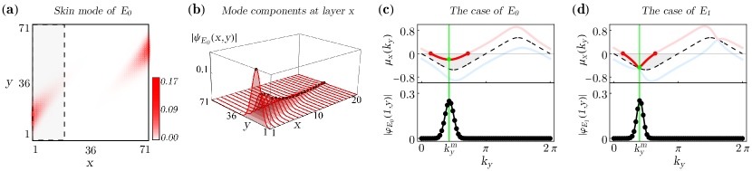
Figure S3:  (a) shows the spatial distribution of skin mode with energy $E_{0}=0.877-0.751i$ in the Hamiltonian Eq.(S5), under the square geometry of size $L_{x}=L_{y}=71$. We extract the components in the first 20 $x$-layers, indicated by the gray area in (a), and present them in (b). (b) clearly shows that the mode components decay and their centers (represented by the black dots) shift with increasing layer $x$. In (c), the upper panel shows the solutions $\mu_{x,1}(k_{y})$ (the blue curve), $\mu_{x,2}(k_{y})$ (the red curve), and the $k_{y}$-dependent GBZ $\tilde{\mu}_{x}(k_{y})$ (the black dashed curve), obtained by solving $\mathcal{H}(\beta,k_{y})-E_{0}=0$. Here the non-Bloch Hamiltonian $\mathcal{H}(\beta)$ is given by Eq.(S17). The green dot represents the minimum of the red opaque arc ended by two Fermi points. The lower panel shows the Fourier transform for the edge-layer ($x$=1) component of the skin mode shown in (a) and (b). (d) follows the same procedure as that in (c), but it is calculated for the energy $E_{1}=-2.867-2.656i$. The system parameters are set to $t=2,\gamma=1$.

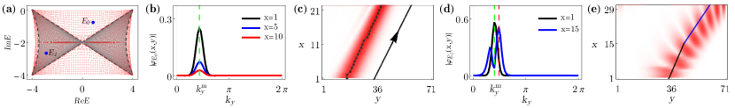
Figure S4:  The relevant calculations corresponding to Fig. S3. (a) shows the OBC eigenvalues (the red dots), including two specific energies $E_{0}=0.877-0.751i$, and $E_{1}=-2.867-2.656i$. (b) presents the Fourier transform of mode components for the energy $E_{0}$ at layers $x=1,5,10$, demonstrating that the momentum center remains invariant as $x$ increases. (c) Correspondingly, for the energy $E_{0}$, the edge-skin mode exhibits constant skewness, which is consistent with the analytical result indicated by the black arrow. (d) For the case of $E_{1}$, the Fourier transform of mode components at layer $x=1,15$ shows a shifting momentum center as $x$ increases. Consequently, the skewness will bend when away from the edge $y$, as illustrated in (e).

The propagator can be calculated according to Cauchy’s integral theorem. For a given energy $E_{0}$, the integral value is determined by the roots of $E_{0}+i0^{+}-\mathcal{H}(\beta_{x},k_{y})=0$. These contributing roots satisfy the following conditions:

• $|\beta_{x}(E_{0},k_{y})|<1$ due to the amplification of mode components in the $-x$ direction;

• $\beta_{x}(E_{0},k_{y})$ is outside the $k_{y}$-dependent GBZ $C_{\beta}(k_{y})$ according to the integral contour in Eq.(S21).

Therefore, the integral value of $\mathcal{G}_{E_{0}}(-x,k_{y})$ is contributed by the roots that are inside the BZ ($|\beta_{x}(k_{y})|\equiv 1$) and outside the $k_{y}$-dependent GBZ ($C_{\beta}(k_{y})$). In terms of $\mu_{x}(E_{0},k_{y})=\log|\beta_{x}(E_{0},k_{y})|$, these contributing roots can be formally expressed as:

$$\mathrm{M}_{x}(E_{0},k_{y}):=\{\mu_{x}(E_{0},k_{y})|\tilde{\mu}_{x}(k_{y})<\mu_{x}(E_{0},k_{y})<0\}.$$ (S22)

For example, we set $E_{0}=0.877-0.751i$. As shown in Fig. S3(c), the region between BZ and $k_{y}$-dependent GBZ is represented by the gray region. The roots, $\mathrm{M}_{x}(E_{0},k_{y})$, contributing to the propagator $\mathcal{G}_{E_{0}}(-x,k_{y})$ are indicated by the red opaque arc in this gray region. Note that the red opaque arc terminates at two Fermi points, as denoted by the red dots in Fig. S3(c).

In the large-size limit, each $k_{y}$ component in $\varphi_{E_{0}}(x_{0},k_{y})$ will amplify in the $-x$ direction. The $k_{y}$ component that gains the maximal amplification corresponds to the minimum in $\mathrm{M}_{x}(E_{0},k_{y})$, which is indicated by the green dot in Fig. S3(c).

$$|\mathcal{G}_{E_{0}}(-x,k_{y})|\propto e^{-\mu_{x,2}(k_{y}^{m})x}.$$ (S23)

Consequently, the momentum center at the edge layer component must be $k_{y}^{m}$, where $\mathrm{M}_{x}(E_{0},k_{y})$ reaches its minimum. Two examples, with $E_{0}=0.877-0.751i$ and $E_{1}=-2.867-2.656i$, are depicted in Fig. S3(c) and (d), respectively. Here, the roots $\mu_{x}(k_{y})$ are presented in the upper panels, and the edge-layer momentum distributions are in the lower panels. These numerical calculations perfectly confirm our conclusion. So far, we have proved that the momentum center of edge-layer component is totally determined by the non-Bloch Hamiltonian $\mathcal{H}(\beta_{x},k_{y})$, without requiring any boundary details.

S-2.2 The skewness of the edge-skin mode

This section complements and extends the discussion on the skewness of the edge-skin mode described in the main text. In the first part, we demonstrate that the skewness manifests differently within two distinct energy spectrum regions and provide additional detailed numerical results. Secondly, we generalize the formula for calculating the skewness to include a more generic case with long-range hopping and offer some numerical examples for verification.

S-2.2.1 The skewness within different energy spectrum regions

Here, we still use the example in Eq.(S9) or its non-Bloch form in Eq.(S17) as our demonstration. It is also the example we used in the main text. The open-boundary eigenvalues are evaluated and represented by the red dots in Fig. S4(a). These OBC eigenvalues can be further divided into two sections by the $k_{y}$-dependent GBZ. According to the non-Bloch Hamiltonian in Eq.(S17), the $k_{y}$-dependent GBZ defined in Eq.(S18) can be calculated as

$$\mathrm{GBZ}_{k_{y}}:=\{(\beta_{x}\equiv r(k_{y})e^{i\theta},k_{y})|k_{y},\theta\in[0,2\pi]\};\quad r(k_{y})=\left|\sqrt{\frac{c_{-}(k_{y})}{c_{+}(k_{y})}}\right|,$$ (S24)

where $c_{\pm}(k_{y})=t\,e^{\pm ik_{y}}+i\gamma$. The $k_{y}$-dependent GBZ can be obtained as $k_{y},\theta\in\mathbb{R}$ run from $0$ to $2\pi$, which is a 2D manifold. Therefore, the spectrum of the $k_{y}$-dependent GBZ can be analytically calculated as

$$\sigma_{\mathrm{cyl}}:=\{\mathcal{H}(\beta_{x},k_{y})|(\beta_{x},k_{y})\in\mathrm{GBZ}_{k_{y}}\},$$ (S25)

which is the gray region included by the black dashed line, as depicted in Fig. S4(a). Consequently, the OBC eigenvalues can be divided into two sections:

$$E_{\text{OBC}}\notin\sigma_{\mathrm{cyl}}\,\,\,\text{and}\,\,\,E_{\text{OBC}}\in\sigma_{\mathrm{cyl}}.$$

As indicated in Fig. S4(a), we select $E_{0}\notin\sigma_{\mathrm{cyl}}$ and $E_{1}\in\sigma_{\mathrm{cyl}}$ as two representative OBC eigenvalues to show the skewness of their corresponding skin modes.

As demonstrated in the previous section, the momentum center of the edge-layer component is determined by the minimum of $\mu_{x}(k_{y})$ in the range between $\mathrm{GBZ}_{k_{y}}$ and BZ, as indicated by the gray region in Fig. S3(c)(d). Using the space-time mapping, $x\rightarrow t$, the skewness of skin mode is mapping into a group velocity of $x$-layer components. Therefore, the initial group velocity (skewness near the edge $y$) can be determined by the momentum center of the edge-layer component. Within this space-time mapping, the complex $-\tilde{k_{x}}=-(k_{x}-i\mu_{x})$ plays the role of ‘complex energy bands’. In this sense, $-\partial_{k_{y}}k_{x}(k_{y})$ represents the group velocity and $\partial_{k_{y}}\mu_{x}(k_{y})$ has the meaning of acceleration of the wavepacket.

In the case of $E_{0}\notin\sigma_{\mathrm{cyl}}$, the $\mu_{x}(k_{y})$ can be solved in Fig. S3(c). At the edge momentum center $k_{y}^{m}$, it satisfies

$$\partial_{k_{y}}\mu_{x,2}(k_{y}^{m})=0.$$ (S26)

It means that wavepacket at the initial time (that is the edge-layer component) has zero acceleration and constant group velocity. In other words, the edge momentum center will not shift as $x$ increases. We show the Fourier transform for layer $x=1,5,10$ in Fig. S4(b). It can be seen that the momentum center is invariant due to the zero acceleration as described in Eq.(S26). The constant group velocity, namely skewness, is calculated as

$$s_{\text{edge{-}y}}(E_{0})=\partial_{k_{y}}k_{x,2}(k_{y}^{m}),$$ (S27)

where $k_{x,i}$ is ordered according to the corresponding $\mu_{x,i}$. As an example, we select $E_{0}=0.877-0.751i$. The first 20 $x$-layer components is shown in Fig. S4(c), where each layer component has been renormalized. The black dots represent the position of maximum amplitude for each layer component. According to formula of skewness in Eq.(S27), the skewness can be analytically calculated as $s_{\text{edge{-}y}}(E_{0})=1.11279$. The analytical result, $\delta y-s_{\text{edge{-}y}}(E_{0})\delta x=0$, is indicated by the black arrow in Fig. S4(c), which agrees well with the numerical results (the direction given by the red trajectory and black dots).

For the case of $E_{1}\in\sigma_{\mathrm{cyl}}$, the edge momentum center is determined by the minimum of $\mu_{x}(k_{y})$ in the range between $\mathrm{GBZ}_{k_{y}}$ and BZ, which is plotted in Fig. S3(d). In this case, the solutions $\mu_{x,i}(k_{y})$ (the red and blue curves) intersect with the $k_{y}$-dependent GBZ (the black dashed curve). It leads to that, the acceleration of edge-layer component is generally nonzero, namely,

$$\partial_{k_{y}}\mu_{x,2}(k_{y}^{m})\neq 0,$$ (S28)

as shown in Fig. S3(d). What it means is that the edge momentum center will be shifted as layer $x$ increases. Consequently, the group velocity varies as as layer $x$ increases. As an example, we select $E_{1}=-2.867-2.656i$. As illustrated in Fig. S4(d), the edge momentum center $k_{y}^{m}$ shifts towards the other two momenta as layer $x$ changes from $x=1$ to $x=15$. For clarity, the momentum distribution at layer $x=15$, namely $\varphi_{E_{1}}(15,k_{y})$, has been renormalized. We denote the momentum center at layer $x=1$ and $x=15$ as $k_{y}^{m}$ and $k_{y}^{1}$, respectively. Correspondingly, the skewness of the skin mode near edge $y$ will bend, as illustrated in Fig. S4(e), where the slopes of the black and blue lines correspond to $\partial_{k_{y}}k_{x,2}(k_{y}^{m})$ and $\partial_{k_{y}}k_{x,2}(k_{y}^{1})$.

S-2.2.2 The skewness in more generic cases

The formula of skewness can be straightforwardly extended into more generic cases with long-range hopping. Without loss of generality, we assume that the skin mode under fully OBCs is localized on the edge $y$. To solve the skewness, the corresponding non-Bloch Hamiltonian can be expressed as

$$\mathcal{H}(\beta_{x},k_{y})=\sum_{l=-m}^{n}c_{l}(k_{y})\beta_{x}^{l},$$ (S29)

where $m$ and $n$ are finite integers representing the hopping range, and $c_{l}(k_{y})$ indicates the $k_{y}$-dependent coefficient. For a given OBC eigenvalue $E_{0}$, we have $(m+n)$ solutions $\mu_{x,i}(k_{y})$, which can be ordered according to their magnitudes $\mu_{x,i}(k_{y})\leq\mu_{x,i+1}(k_{y})$. Based on the 1D non-Bloch theorem, the $k_{y}$-dependent GBZ can be expressed as

$$\tilde{\mu}_{x}(k_{y})\equiv\mu_{x,m}(E_{0},k_{y})=\mu_{x,m+1}(E_{0},k_{y}),$$ (S30)

which is the direct extension of Eq.(S19). Therefore, for the case of $E_{0}\notin\sigma_{\mathrm{cyl}}$, the corresponding solutions can be ordered as:

$$\mu_{x,1}(E_{0},k_{y})\leq\dots\leq\tilde{\mu}_{x}(k_{y})<\mu_{x,m+1}(E_{0},k_{y})\leq\dots\mu_{x,m+n}(E_{0},k_{y}).$$ (S31)

In the same way, we can extend the first conclusion of skewness as: The momentum center of the edge-layer component is determined by the minimum of $\mu_{x,m+1}(E_{0},k_{y})$, denoted as $k_{y}^{m}$. Consequently, the edge-layer component satisfies

$$\partial_{k_{y}}\mu_{x,m+1}(k_{y}^{m})=0$$ (S32)

due to $E_{0}\notin\sigma_{\mathrm{cyl}}$, which represents the generalization of Eq.(S26). Accordingly, the skewness of edge-skin mode with energy $E_{0}$ can be further extended as

$$s_{\mathrm{edge{-}y}}(E_{0})=\partial_{k_{y}}k_{x,m+1}(k_{y}^{m}),$$ (S33)

where $k_{x,i}$ has been ordered corresponding to $\mu_{x,i}$.

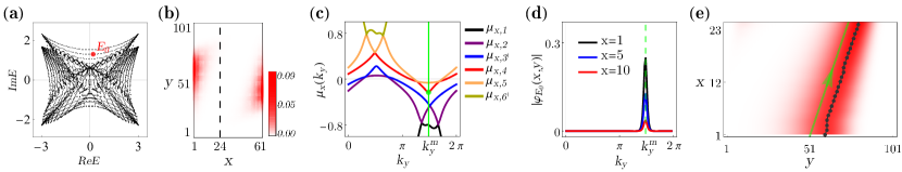
Figure S5:  The skewness in a generic Hamiltonian given by Eq.(S36). (a) represents the OBC eigenvalues of the Hamiltonian with system size $L_{x}=61$ and $L_{y}=101$. (b) The spatial distribution of skin mode with energy $E_{0}=0.212+1.295i$, indicated by the red dot in (a). The black dashed line refers to the layer $x=24$. (c) The six solutions, $\mu_{x,i}(k_{y})$, have been ordered according to their amplitudes. The green dot denotes the minimum of $\mu_{x,4}(k_{y})$, which is also the minimum value within the range between the $k_{y}$-dependent GBZ, as defined in Eq.(S30) (not shown here), and the BZ, where $\mu_{x}(k_{y})\equiv 0$. (d) The Fourier transform of mode components at layer $x=1,5,10$ shows a constant momentum center as $x$ increases. (e) The edge-skin mode of energy $E_{0}$ exhibits constant skewness, as shown by the black dots, which is consistent with the analytical result $s_{\mathrm{edge}{-}y}(E_{0})=0.9784$, as indicated by the green arrow.

Here, we present a generic numerical example to support the above generalization for the skewness of edge-skin mode. The non-Bloch Hamiltonian with real-valued edge momenta is given by

$$\mathcal{H}(\beta_{x},k_{y})=\frac{-i(\beta_{x}^{3}+\beta_{x}^{-3})}{3}+\frac{i(\beta_{x}+\beta_{x}^{-1})}{6}+(i-\frac{3}{2}e^{ik_{y}})\beta_{x}^{2}+(i-\frac{3}{2}e^{-ik_{y}})\beta_{x}^{-2}.$$ (S34)

The bulk Hamiltonian has reciprocity, $\mathcal{H}(\beta_{x},k_{y})=\mathcal{H}(1/\beta_{x},-k_{y})$. The OBC eigenvalues, calculated for a system size of $L_{x}=61$ and $L_{y}=101$, are represented by black dots in Fig.S5(a). For illustration, we calculate the skewness of the skin mode with energy $E_{0}=0.212+1.295i$ (the red dot in Fig. S5(a)). The spatial distribution of the wavefunction is plotted in Fig. S5(b), where the black dashed line refers to the layer $x=24$. The wavefunction is symmetrically localized at the two edges in the $y$ direction. For the given $E_{0}$, we obtain the solutions $\mu_{x,i=1,\dots,6}(k_{y})$ by solving $\mathcal{H}(\beta_{x},k_{y})-E_{0}=0$. These solutions are ordered by their amplitudes, $\mu_{x,i}(k_{y})\leq\mu_{x,i+1}(k_{y})$, and are illustrated in Fig. S5(c). Since $E_{0}\in\sigma_{\mathrm{cyl}}$, there exists a ‘gap’ between $\mu_{x,3}(k_{y})$ (the blue curve) and $\mu_{x,4}(k_{y})$ (the red curve). The $k_{y}$-dependent GBZ, $\tilde{\mu}(k_{y})\equiv\mu_{x,3}(E,k_{y})=\mu_{x,4}(E,k_{y})$, lies within this gap (not depicted here).

According to our conclusion, the momentum center of the edge-layer component is determined by the minimum of $\mu_{x,4}(k_{y})$, as indicated by the green dot in Fig. S5(c). At the momentum $k_{y}^{m}$, $\mu_{x,4}(k_{y})$ reaches its minimum and satisfies the condition

$$\partial_{k_{y}}\mu_{x,4}(k_{y}^{m})=0,$$

which suggests that the edge momentum center remains unchanged as layer $x$ increases. This is verified in Fig. S5(d), where the Fourier transform of layer components at $x=1,5,10$ is shown, and the momentum centers consistently lie at $k_{y}^{m}$. Therefore, the skewness of the skin mode with energy $E_{0}$ is formulated as

$$s_{\mathrm{edge{-}y}}(E_{0})=\partial_{k_{y}}k_{x,4}(k_{y}^{m}),$$

and analytically calculated to be $s_{\mathrm{edge{-}y}}(E_{0})=0.9784$ for $E_{0}=0.212+1.295i$. The analytical result, $\delta y-s_{\mathrm{edge{-}y}}(E_{0})\delta x=0$ indicated by the green arrow in Fig. S5(e), perfectly matches the numerical result, the direction given by the black dots.

S-3 The anomalous spectral sensitivity in the edge-skin effect

In this section, we show that in the edge-skin effect, the spectrum under a specified cylinder geometry is highly sensitive to the perturbations that break the fragile reciprocity, such as the weak onsite disorders. For example, when the edge $y$ is the localized edge of the skin modes, we specify the cylinder geometry as that with PBC in the $y$ and OBC in the $x$ direction. Based on this, the inversion or reciprocity symmetry in the edge-skin effect, given by Eq.(S5), further requires the characteristic equation to satisfy

$$f_{E}(k_{x},\mu_{x},k_{y})=f_{E}(-k_{x},-\mu_{x},-k_{y})=0,$$ (S35)

which is termed fragile reciprocity. The fragile reciprocity can be easily broken by the perturbations that break the translation symmetry in the $y$ direction, such as on-site disorders or open boundaries, thus termed ‘fragile’.

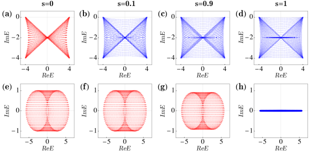
Figure S6:  In the cases of the edge-skin effect (a)-(d) and corner-skin effect (e)-(h), the energy spectra change as the boundary conditions transition from cylinder geometry (a)(e) to fully open-boundary geometry (d)(h). The non-perturbative phenomenon in the spectrum occurs near the cylinder geometry in the case of edge-skin effect, as demonstrated by (a)(b), whereas it occurs near the fully open-boundary geometry in the case of corner-skin effect, as evidenced by (g)(h).

Here, we numerically demonstrate that the spectral sensitivity is anomalous and unique to the edge-skin effect, distinguishing it from the corner-skin effect. The edge-skin effect is exemplified by

$$h_{\mathrm{ESE}}(\bm{k})=4\cos(k_{x}+k_{y})-2i(1-\cos{k_{x}}),$$

as given by Eq.(S9). We start with the Hamiltonian under the cylinder geometry, that is, PBC in $y$ and OBC in $x$ direction. Modulating the strength of the boundary link $s$ in the $y$ direction allows for a transition from cylinder geometry ($s=0$) to fully OBC geometry ($s=1$). Therefore, the set of Hamiltonians is formally expressed as

$$H_{s}=H_{\mathrm{cyl}}-sH_{\mathrm{B}},$$ (S36)

where $H_{\mathrm{cyl}}$ denotes the cylinder-geometry Hamiltonian, and $H_{\mathrm{B}}$ represents the boundary link term. Therefore, $H_{0}$ refers to the Hamiltonian under cylinder geometry, and $H_{1}$ corresponds to the Hamiltonian under fully OBCs. The spectra corresponding to different boundary links are depicted in Fig. S6(a)-(d). Notably, a minor adjustment of the boundary link ($s=0.1$) can lead to a substantial alteration of the spectrum, as evidenced by the comparison between Fig. S6(a) and (b). Moreover, the energy spectrum in Fig. S6(b) closely resembles the fully open-boundary spectrum in Fig. S6(d).

The Hamiltonian for the corner-skin effect is given by

$$h_{\mathrm{CSE}}(\bm{k})=3(\cos{k_{x}}+\cos{k_{y}})+i(\sin{k_{x}}+\sin{k_{y}}).$$

The energy spectra corresponding to different boundary links are illustrated in Fig. S6(e)-(h). In the corner-skin effect, the minor modification of boundary link can be considered as a perturbation to its energy spectra, as displayed in Fig. S6(e)-(g). The non-perturbative effect in the spectrum occurs near the fully OBC spectrum owing to the change of the GBZ condition Yang et al. (2020); Li et al. (2020), as illustrated in Fig. S6(g) and (h).

References

- Shen et al. (2018) H. Shen, B. Zhen, and L. Fu, Phys. Rev. Lett. 120, 146402 (2018).
- Gong et al. (2018) Z. Gong, Y. Ashida, K. Kawabata, K. Takasan, S. Higashikawa, and M. Ueda, Phys. Rev. X 8, 031079 (2018).
- Kawabata et al. (2019) K. Kawabata, K. Shiozaki, M. Ueda, and M. Sato, Phys. Rev. X 9, 041015 (2019).
- Ashida et al. (2020) Y. Ashida, Z. Gong, and M. Ueda, Advances in Physics 69, 249 (2020).
- Bergholtz et al. (2021) E. J. Bergholtz, J. C. Budich, and F. K. Kunst, Rev. Mod. Phys. 93, 015005 (2021).
- Okuma and Sato (2023) N. Okuma and M. Sato, Annual Review of Condensed Matter Physics 14, 83 (2023), https://doi.org/10.1146 annurev-conmatphys-040521-033133 .
- Feng et al. (2017) L. Feng, R. El-Ganainy, and L. Ge, Nature Photonics 11, 752 (2017).
- Scheibner et al. (2020) C. Scheibner, A. Souslov, D. Banerjee, P. Surówka, W. T. M. Irvine, and V. Vitelli, Nature Physics 16, 475 (2020).
- Song et al. (2019a) F. Song, S. Yao, and Z. Wang, Phys. Rev. Lett. 123, 170401 (2019a).
- Nagai et al. (2020) Y. Nagai, Y. Qi, H. Isobe, V. Kozii, and L. Fu, Phys. Rev. Lett. 125, 227204 (2020).
- Yao and Wang (2018) S. Yao and Z. Wang, Phys. Rev. Lett. 121, 086803 (2018).
- Martinez Alvarez et al. (2018) V. M. Martinez Alvarez, J. E. Barrios Vargas, and L. E. F. Foa Torres, Phys. Rev. B 97, 121401(R) (2018).
- Lee and Thomale (2019) C. H. Lee and R. Thomale, Phys. Rev. B 99, 201103(R) (2019).
- Lee et al. (2019a) C. H. Lee, L. Li, and J. Gong, Phys. Rev. Lett. 123, 016805 (2019a).
- Zhang et al. (2020) K. Zhang, Z. Yang, and C. Fang, Phys. Rev. Lett. 125, 126402 (2020).
- Okuma et al. (2020) N. Okuma, K. Kawabata, K. Shiozaki, and M. Sato, Phys. Rev. Lett. 124, 086801 (2020).
- Yi and Yang (2020) Y. Yi and Z. Yang, Phys. Rev. Lett. 125, 186802 (2020).
- Li et al. (2020a) L. Li, C. H. Lee, S. Mu, and J. Gong, Nature Communications 11, 5491 (2020a).
- Kawabata et al. (2020a) K. Kawabata, M. Sato, and K. Shiozaki, Phys. Rev. B 102, 205118 (2020a).
- Zirnstein et al. (2021) H.-G. Zirnstein, G. Refael, and B. Rosenow, Phys. Rev. Lett. 126, 216407 (2021).
- Guo et al. (2021) C.-X. Guo, C.-H. Liu, X.-M. Zhao, Y. Liu, and S. Chen, Phys. Rev. Lett. 127, 116801 (2021).
- Wang et al. (2023a) Z.-Y. Wang, J.-S. Hong, and X.-J. Liu, Phys. Rev. B 108, L060204 (2023a).
- Schindler et al. (2023) F. Schindler, K. Gu, B. Lian, and K. Kawabata, PRX Quantum 4, 030315 (2023).
- Denner et al. (2023) M. M. Denner, T. Neupert, and F. Schindler, Journal of Physics: Materials 6, 045006 (2023).
- Lin et al. (2023) R. Lin, T. Tai, L. Li, and C. H. Lee, Frontiers of Physics 18, 53605 (2023).
- Zhang et al. (2022a) X. Zhang, T. Zhang, M.-H. Lu, and Y.-F. Chen, Advances in Physics: X 7, 2109431 (2022a).
- Lee (2016) T. E. Lee, Phys. Rev. Lett. 116, 133903 (2016).
- Kunst et al. (2018) F. K. Kunst, E. Edvardsson, J. C. Budich, and E. J. Bergholtz, Phys. Rev. Lett. 121, 026808 (2018).
- Borgnia et al. (2020) D. S. Borgnia, A. J. Kruchkov, and R.-J. Slager, Phys. Rev. Lett. 124, 056802 (2020).
- Zhang et al. (2021a) W. Zhang, X. Ouyang, X. Huang, X. Wang, H. Zhang, Y. Yu, X. Chang, Y. Liu, D.-L. Deng, and L.-M. Duan, Phys. Rev. Lett. 127, 090501 (2021a).
- McDonald et al. (2018) A. McDonald, T. Pereg-Barnea, and A. A. Clerk, Phys. Rev. X 8, 041031 (2018).
- Lee et al. (2019b) J. Y. Lee, J. Ahn, H. Zhou, and A. Vishwanath, Phys. Rev. Lett. 123, 206404 (2019b).
- Bessho and Sato (2021) T. Bessho and M. Sato, Phys. Rev. Lett. 127, 196404 (2021).
- Liang et al. (2022) Q. Liang, D. Xie, Z. Dong, H. Li, H. Li, B. Gadway, W. Yi, and B. Yan, Phys. Rev. Lett. 129, 070401 (2022).
- Zhang et al. (2023) K. Zhang, C. Fang, and Z. Yang, Phys. Rev. Lett. 131, 036402 (2023).
- Porras and Fernández-Lorenzo (2019) D. Porras and S. Fernández-Lorenzo, Phys. Rev. Lett. 122, 143901 (2019).
- Longhi (2019) S. Longhi, Phys. Rev. Research 1, 023013 (2019).
- Longhi (2020) S. Longhi, Phys. Rev. Lett. 124, 066602 (2020).
- Xue et al. (2021) W.-T. Xue, M.-R. Li, Y.-M. Hu, F. Song, and Z. Wang, Phys. Rev. B 103, L241408 (2021).
- Li et al. (2021) L. Li, S. Mu, C. H. Lee, and J. Gong, Nature Communications 12, 5294 (2021).
- Sun et al. (2021) X.-Q. Sun, P. Zhu, and T. L. Hughes, Phys. Rev. Lett. 127, 066401 (2021).
- Kawabata et al. (2021) K. Kawabata, K. Shiozaki, and S. Ryu, Phys. Rev. Lett. 126, 216405 (2021).
- Lu et al. (2021) M. Lu, X.-X. Zhang, and M. Franz, Phys. Rev. Lett. 127, 256402 (2021).
- Longhi (2022) S. Longhi, Phys. Rev. Lett. 128, 157601 (2022).
- Xue et al. (2022) W.-T. Xue, Y.-M. Hu, F. Song, and Z. Wang, Phys. Rev. Lett. 128, 120401 (2022).
- Fang et al. (2023) Z. Fang, C. Fang, and K. Zhang, Phys. Rev. B 108, 165132 (2023).
- Yokomizo and Murakami (2019) K. Yokomizo and S. Murakami, Phys. Rev. Lett. 123, 066404 (2019).
- Yang et al. (2020) Z. Yang, K. Zhang, C. Fang, and J. Hu, Phys. Rev. Lett. 125, 226402 (2020).
- Song et al. (2019b) F. Song, S. Yao, and Z. Wang, Phys. Rev. Lett. 123, 246801 (2019b).
- Deng and Yi (2019) T.-S. Deng and W. Yi, Phys. Rev. B 100, 035102 (2019).
- Kawabata et al. (2020b) K. Kawabata, N. Okuma, and M. Sato, Phys. Rev. B 101, 195147 (2020b).
- Helbig et al. (2020) T. Helbig, T. Hofmann, S. Imhof, M. Abdelghany, T. Kiessling, L. W. Molenkamp, C. H. Lee, A. Szameit, M. Greiter, and R. Thomale, Nature Physics 16, 747 (2020).
- Ghatak et al. (2020) A. Ghatak, M. Brandenbourger, J. van Wezel, and C. Coulais, Proceedings of the National Academy of Sciences 117, 29561 (2020).
- Xiao et al. (2020) L. Xiao, T. Deng, K. Wang, G. Zhu, Z. Wang, W. Yi, and P. Xue, Nature Physics 16, 761 (2020).
- Wang et al. (2021) K. Wang, T. Li, L. Xiao, Y. Han, W. Yi, and P. Xue, Phys. Rev. Lett. 127, 270602 (2021).
- Yao et al. (2018) S. Yao, F. Song, and Z. Wang, Phys. Rev. Lett. 121, 136802 (2018).
- Liu et al. (2019) T. Liu, Y.-R. Zhang, Q. Ai, Z. Gong, K. Kawabata, M. Ueda, and F. Nori, Phys. Rev. Lett. 122, 076801 (2019).
- Li et al. (2020b) L. Li, C. H. Lee, and J. Gong, Phys. Rev. Lett. 124, 250402 (2020b).
- Zhang et al. (2022b) K. Zhang, Z. Yang, and C. Fang, Nature Communications 13, 2496 (2022b).
- Wang et al. (2022a) Y.-C. Wang, J.-S. You, and H. H. Jen, Nature Communications 13, 4598 (2022a).
- Qin et al. (2023) Y. Qin, K. Zhang, and L. Li, Geometry-dependent skin effect and anisotropic bloch oscillations in a non-hermitian optical lattice (2023), arXiv:2304.03792 .
- Zou et al. (2021) D. Zou, T. Chen, W. He, J. Bao, C. H. Lee, H. Sun, and X. Zhang, Nature Communications 12, 7201 (2021).
- Zhang et al. (2021b) X. Zhang, Y. Tian, J.-H. Jiang, M.-H. Lu, and Y.-F. Chen, Nature Communications 12, 5377 (2021b).
- Zhou et al. (2023) Q. Zhou, J. Wu, Z. Pu, J. Lu, X. Huang, W. Deng, M. Ke, and Z. Liu, Nature Communications 14, 4569 (2023).
- Wang et al. (2023b) W. Wang, M. Hu, X. Wang, G. Ma, and K. Ding, Phys. Rev. Lett. 131, 207201 (2023b).
- Wan et al. (2023) T. Wan, K. Zhang, J. Li, Z. Yang, and Z. Yang, Science Bulletin 68, 2330 (2023).
- Jiang and Lee (2023) H. Jiang and C. H. Lee, Phys. Rev. Lett. 131, 076401 (2023).
- Yokomizo and Murakami (2023) K. Yokomizo and S. Murakami, Phys. Rev. B 107, 195112 (2023).
- Wang et al. (2022b) H.-Y. Wang, F. Song, and Z. Wang, Amoeba formulation of the non-hermitian skin effect in higher dimensions (2022b), arXiv:2212.11743 .
- Hu (2023) H. Hu, Non-hermitian band theory in all dimensions: uniform spectra and skin effect (2023), arXiv:2306.12022 .
- Note (1) The edge momenta refer to the momenta along the direction of the localization edge.
- Note (2) Since the Hamiltonian only respects inversion symmetry and lacks mirror symmetries, a convenient criterion to determine the OBC geometry where localization vanishes for a given wavefunction with energy remains unclear.
- Note (3) The OBC spectrum is always covered by the PBC spectrum in the complex energy plane, hence the equation always have solutions.
- Yang et al. (2021) Z. Yang, A. P. Schnyder, J. Hu, and C.-K. Chiu, Phys. Rev. Lett. 126, 086401 (2021).
- (75) See Supplemental Material for more details .
- Bernevig (2013) B. A. Bernevig, Topological insulators and topological superconductors (Princeton university press, 2013).
- Note (4) Although Fermi-arc states are frequently discussed in Hermitian chiral semimetals with semi-infinite boundary conditions, fully OBCs, especially with specific geometries, are more relevant to realistic materials. Under fully OBCs, the degenerate Fermi-arc states become split, yet several zero-energy edge states remain. However, the characteristics of these zero modes are largely unexplored.
- Mao et al. (2021) L. Mao, T. Deng, and P. Zhang, Phys. Rev. B 104, 125435 (2021).

References

- Wang et al. (2022) H.-Y. Wang, F. Song, and Z. Wang, Amoeba formulation of the non-hermitian skin effect in higher dimensions (2022), arXiv:2212.11743 .
- Hu (2023) H. Hu, Non-hermitian band theory in all dimensions: uniform spectra and skin effect (2023), arXiv:2306.12022 .
- Zhang et al. (2020) K. Zhang, Z. Yang, and C. Fang, Phys. Rev. Lett. 125, 126402 (2020).
- Okuma et al. (2020) N. Okuma, K. Kawabata, K. Shiozaki, and M. Sato, Phys. Rev. Lett. 124, 086801 (2020).
- Kawabata et al. (2020) K. Kawabata, N. Okuma, and M. Sato, Phys. Rev. B 101, 195147 (2020).
- Yi and Yang (2020) Y. Yi and Z. Yang, Phys. Rev. Lett. 125, 186802 (2020).
- Bernevig (2013) B. A. Bernevig, Topological insulators and topological superconductors (Princeton university press, 2013).
- Gong et al. (2018) Z. Gong, Y. Ashida, K. Kawabata, K. Takasan, S. Higashikawa, and M. Ueda, Phys. Rev. X 8, 031079 (2018).
- Kawabata et al. (2019) K. Kawabata, K. Shiozaki, M. Ueda, and M. Sato, Phys. Rev. X 9, 041015 (2019).
- Mao et al. (2021) L. Mao, T. Deng, and P. Zhang, Phys. Rev. B 104, 125435 (2021).
- Yao and Wang (2018) S. Yao and Z. Wang, Phys. Rev. Lett. 121, 086803 (2018).
- Yokomizo and Murakami (2019) K. Yokomizo and S. Murakami, Phys. Rev. Lett. 123, 066404 (2019).
- Yang et al. (2020) Z. Yang, K. Zhang, C. Fang, and J. Hu, Phys. Rev. Lett. 125, 226402 (2020).
- Li et al. (2020) L. Li, C. H. Lee, S. Mu, and J. Gong, Nature Communications 11, 5491 (2020).