Stroke-based Neural Painting and Stylization with Dynamically Predicted Painting Region

Abstract.

Stroke-based rendering aims to recreate an image with a set of strokes. Most existing methods render complex images using an uniform-block-dividing strategy, which leads to boundary inconsistency artifacts. To solve the problem, we propose Compositional Neural Painter, a novel stroke-based rendering framework which dynamically predicts the next painting region based on the current canvas, instead of dividing the image plane uniformly into painting regions. We start from an empty canvas and divide the painting process into several steps. At each step, a compositor network trained with a phasic RL strategy first predicts the next painting region, then a painter network trained with a WGAN discriminator predicts stroke parameters, and a stroke renderer paints the strokes onto the painting region of the current canvas. Moreover, we extend our method to stroke-based style transfer with a novel differentiable distance transform loss, which helps preserve the structure of the input image during stroke-based stylization. Extensive experiments show our model outperforms the existing models in both stroke-based neural painting and stroke-based stylization. Code is available at: https://github.com/sjtuplayer/Compositional_Neural_Painter.

1. Introduction

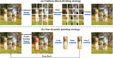
Figure 1. (a) The painting process of existing models (Huang et al., 2019; Liu et al., 2021a; Zou et al., 2021) which uniformly divide the image plane into $k\times k$ blocks and paint each block independently, resulting in boundary inconsistency artifacts between each two adjacent blocks; (b) The painting process of our model: we dynamically predict the next painting region (red box) and paint it with our painter network, which avoids the boundary inconsistency artifacts and reconstructs more details in the target image.

Stroke-based rendering (SBR) aims to recreate an image with a set of brushstrokes. Different from mainstream generation models based on VAE  (Kingma and Welling, 2013), GANs  (Goodfellow et al., 2014) and Diffusion model  (Ho et al., 2020), which generate images using pixels as basic elements, SBR uses brushstrokes as basic elements and decomposes the painting process into a stroke sequence. By painting the strokes sequentially onto the canvas, SBR can better imitate the painting process of human artists.

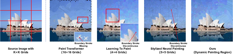
Figure 2. The boundary inconsistency artifacts of the existing methods with 3,000 strokes: Paint Transformer  (Liu et al., 2021a), Learning To Paint  (Huang et al., 2019) and Stylized Neural Painting  (Zou et al., 2021). All the methods suffer from the discontinuous strokes at the junction of the adjacent blocks. Please zoom in for details.

Traditional SBR methods  (Hertzmann, 1998; Litwinowicz, 1997; Turk and Banks, 1996; Haeberli, 1990; Teece, 1998; Ganin et al., 2018; Zhou et al., 2018; Tong et al., 2022) rely on non-deep learning methods, e.g., greedy searching and heuristic optimization with low efficiency. Recent deep learning-based methods can be classified into three classes: RL-based methods  (Huang et al., 2019; Singh and Zheng, 2021; Singh et al., 2022), DL-based methods  (Liu et al., 2021a) and optimization-based methods  (Zou et al., 2021; Kotovenko et al., 2021). All the existing methods can only predict a limited number of strokes for an input image block, since more strokes require much more training or optimization resources. But the images in real world (e.g., images in ImageNet  (Deng et al., 2009)) are usually too complex to reconstruct with limited strokes. To render more details, existing methods  (Huang et al., 2019; Liu et al., 2021a; Zou et al., 2021) uniformly partition the image plane into $k\times k$ blocks and predict strokes for each block independently. However, this uniform-block-dividing strategy (Fig. 1(a)) suffers from the following weaknesses: (1) it is only used in their testing stage, which makes their testing setting inconsistent with their training setting; (2) it leads to boundary inconsistency artifacts (Fig. 2), i.e., since each block is rendered separately, the blindness to adjacent blocks leads to inconsistent strokes on the two sides of the block boundary.

Inspired by the real painting process, where artists usually decide the painting region first, and then draw the objects in the corresponding region, we propose Compositional Neural Painter, a novel stroke-based rendering framework with a painting scheme that first predicts “where to paint” and then decides “what to paint”. Compared to Intelli-Paint (Singh et al., 2022) which employs sliding attention window to guide the painting process in the local foreground object region and strongly relies on the object detection method, our model can predict the painting regions in a global view and is free from reliance on any object detection models. This allows our model to be more robust and effective in handling scenarios with multiple or no clearly defined foreground objects

In detail, our model is composed of two parts: a compositor network predicting “where to paint” and a painter network decides “what to paint”. The compositor network is proposed to dynamically predict the next painting region based on the current canvas (Fig. 1(b)), instead of dividing the image plane uniformly into painting regions. We start from an empty canvas and decompose the painting process into several steps. At each step, the compositor network first predicts the next painting region, a painter network then predicts the stroke parameters, and a stroke renderer paints the strokes onto the painting region of the canvas. Specifically, the compositor network is trained with a RL strategy with phasic reward function; and the painter network is a CNN-based model trained with a WGAN discriminator to penalize always painting similar strokes, which often happens without using RL strategy. Furthermore, we extend our method to stroke-based stylization with a novel differentiable distance transform loss, which helps preserve the structure of the input image during stroke-based stylization.

The contributions of our work are three-fold:

• We propose Compositional Neural Painter, a novel stroke-based rendering model which dynamically predicts the next painting region based on the current canvas. This dynamic rendering strategy solves the boundary inconsistency artifacts caused by the uniformly divided painting regions in existing methods and achieves good painting performance.

• We propose a compositor network trained with a phasic RL strategy to predict the next painting region, a painter network trained with a WGAN discriminator to forecast the stroke parameters in the predicted painting region, and a neural renderer for stroke rendering.

• We extend our method to stroke-based style transfer task with a novel differentiable distance transform loss, which helps preserve the structure of the input image during stroke-based stylization.

2. Related Works

Stroke-based rendering (SBR). Stroke-based image rendering (SBR) aims at recreating a target image with a set of brushstrokes. Different from the general image synthesising models (e.g., VAE  (Kingma and Welling, 2013), GANs  (Goodfellow et al., 2014) and Diffusion Models  (Ho et al., 2020)) which generate images using pixels as basic elements, SBR methods emulates the real painting process of human artists, employing brushstrokes as the fundamental unit to paint stroke-by-stroke, thereby enhancing the fidelity of the painted images in terms of local texture and brushstroke details to that of real artistic works. The traditional SBR algorithms either employ greedy search  (Hertzmann, 1998; Litwinowicz, 1997; Tong et al., 2022), devise heuristic optimization  (Turk and Banks, 1996), or require user inputs  (Haeberli, 1990; Teece, 1998) to find the position and other characteristics of each stroke. Among them, Im2Oil (Tong et al., 2022) is the latest method, which incorporates adaptive sampling and greedy search based on probability density maps, resulting in superior painting results. With the development of deep learning in recent years, many SBR methods based on neural networks have been proposed. Early works  (Graves, 2013; Ha and Eck, 2017) employed recurrent neural networks (RNN) to decompose the image into brushstrokes. However, the demand for manual annotation limits their application.  Ganin et al. (2018) and  Zhou et al. (2018) introduced reinforcement learning (RL) to synthesize stroke sequences, but can only render simple images like sketches.

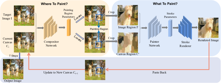
Figure 3. Model framework of our Compositional Neural Painter: Our model consists of a compositor network, a painter network and a stroke renderer. We start from an empty canvas and decompose the painting process into T steps. At each step $t$, the compositor network first predicts the painting region parameters $r_{t}$, then the painter network estimates the strokes parameters $s_{t}$ and the stroke renderer paints the strokes constructed from $s_{t}$ onto the painting region $r$ of the current canvas $C_{t}$. After T steps, our model output the painting constructed by a set of strokes.

To paint a complex real-world images using stroke-based rendering,  Huang et al. (2019) employed a more complicated RL model DDPG  (Lillicrap et al., 2015) with a WGAN  (Arjovsky et al., 2017) reward. To improve the reconstruction ability,  Singh and Zheng (2021) and  Singh et al. (2022) introduced semantic guidance into the RL model, making it concentrate more on the main object in the image. Specifically, Intelli-Paint (Singh et al., 2022) predicts both attention window and stroke parameters in one network to better imitate human painting process, but its heavy reliance on object detection and the limited RL training efficiency restricts its ability in painting complex images and predicting enough strokes for fine-grained details. To solve the low-training efficiency of the RL-based methods,  Liu et al. (2021a) then proposed a RL-free model Paint Transformer, which accelerates the training stage and achieves better training stability. Besides the learning-based methods, some optimization-based methods  (Zou et al., 2021; Kotovenko et al., 2021) decomposed the images into a series of parameterized strokes through iterative optimization process. But they suffer from a long optimization time for each image. Although the above methods can achieve a relatively good result in real image rendering, they either suffer from the boundary inconsistency artifacts, or lack the ability to render a more complex image. In contrast, we employ a compositor network to dynamically predict the next paint region and then paint by a painter network, which not only solves the boundary inconsistency artifacts, but also achieves a better reconstruction quality. Moreover, in contrast to Intelli-Paint(Singh et al., 2022), which utilizes sliding attention windows to guide the painting process in the foreground object region and heavily relies on object detection, our two-stage painting approach has the ability to paint significantly more intricate details without the need of object detection.

Stroke-based style transfer. Style transfer aims at transferring the style from a style image to a content image. Previous style transfer methods  (Gatys et al., 2016; Huang and Belongie, 2017; Cao et al., 2018; Liu et al., 2021b; Song et al., 2021) confined the stylization process in the pixel domain. stroke-based style transfer methods  (Zou et al., 2021; Kotovenko et al., 2021) stylized images using brushstrokes as the basic element, optimizing stroke parameters instead of pixels. However, the existing stroke-based style transfer methods cannot preserve of the structure of the input image well. Different from these methods, we design a new stroke-based stylization framework with a novel differentiable distance transform loss, which can preserve the structure of the input image during stroke-based stylization.

3. Method

3.1. Overview

Stroke-based rendering aims at recreating an image using strokes as basic painting elements. Existing methods  (Huang et al., 2019; Liu et al., 2021a; Zou et al., 2021; Singh and Zheng, 2021, 2021; Singh et al., 2022) predict a limited number of strokes for an input image block, since more strokes require much more training or optimization resources. But the images in real world are usually too complex to reconstruct with limited strokes. To render more details, existing methods  (Huang et al., 2019; Liu et al., 2021a; Zou et al., 2021) uniformly partition the image plane into $k\times k$ blocks, and predict stroke parameters for each block independently. However, this uniform-block-dividing strategy in the test stage leads to boundary inconsistency artifacts: since the strokes of each image block are predicted separately, the blindness to the adjacent blocks leads to inconsistent strokes on the two sides of the block boundary. Fig. 2 shows some examples of the boundary inconsistency artifacts, including stroke-discontinuous and stroke-missing problem. Besides, the semantic-based methods (Singh and Zheng, 2021; Singh et al., 2022) abandon uniform-block-dividing strategy and concentrate on the foregrounds by painting more strokes. But their heavy reliance on object detection and the low RL-training efficiency restrict their ability in painting complex images with multiple or no clearly defined objects.

To solve these problems, we propose Compositional Neural Painter, a novel stroke-based rendering model that dynamically predicts the next painting region based on the current canvas. By dynamically deciding the painting region instead of uniformly partition, our method can better reconstruct details and solve the boundary inconsistency problems. Our Compositional Neural Painter consists of three modules: 1) a compositor network that takes a target image $I$ and a canvas $C$ as inputs and predicts the next painting region $r$ ; 2) a painter network that takes the cropped target image $I^{r}$ and the cropped canvas $C^{r}$ according to region $r$ as inputs, and predicts the stroke parameters $s$; 3) a stroke renderer that renders the strokes of parameters $s$ back into the current canvas.

We start from an empty canvas $C_{0}$ and decompose the painting process into $T$ steps (Fig. 3). At each step $t$, the compositor network first predicts the painting region $r_{t}$, then the painter network estimates the strokes parameters $s_{t}$ for $N$ strokes, and the stroke renderer paints the strokes constructed from $s_{t}$ onto the painting region $r$ of the current canvas $C_{t}$. After $T$ steps, we get a final rendered image $I_{r}=C_{T}$ made up of sequentially painted brushstrokes, which resembles the target image $I$.

3.2. Compositor Network: Where To Paint?

In real painting process, human artists usually decide where to paint first based on the current canvas, and then paint the strokes in the corresponding painting region, instead of painting from top left to right down. Inspired by this, we design the painting process of a set of strokes as human artists do: first predicting “where to paint” and then deciding “what to paint”. To solve the first question, we design a compositor network, which dynamically predicts the next painting region based on the current canvas, instead of uniformly partitioning the image plane into painting regions. The compositor network has a global sight of the painting and guides the whole model to paint in a coarse-to-fine manner.

Model framework. At each step $t$, the compositor network takes a target image $I$ and a current canvas $C_{t}$ as inputs to predict the painting region $r_{t}$ indicating where should be painted next. The painting region is a rectangular region denoted by $r_{t}=(x,y,w,h)$, where $(x,y)$ refers to the upper-left endpoint coordinate, and $(w,h)$ denote the width and height. After predicting the painting region $r_{t}$, the painter network and stroke renderer will predict the stroke parameters for this region and render the strokes onto the current canvas to get a new canvas $C_{t+1}$.

Training strategy. Previous works train the neural painting networks based on self-supervision (Huang et al., 2019; Singh and Zheng, 2021; Liu et al., 2021a; Singh et al., 2022) (minimizing the distance between the rendered image and input image). However, since our painting process needs to crop the canvas according to the predicted painting region, the predicted parameters $(x,y,w,h)$ need to be rounded to the nearest integers. Due to the non-differentiable rounding operation, deep learning strategies based on back propagation are not applicable to train the compositor network. Therefore, we introduce a Reinforcement Learning (RL) framework DDPG  (Lillicrap et al., 2015) to train the compositor network.

The original reward function $R$ used in DDPG-based RL methods  (Huang et al., 2019; Singh and Zheng, 2021) is formulated as:

(1) $$R_{ori}=\frac{\|I-C_{t}\|_{2}}{\|I\|_{2}}-\frac{\|I-C_{t+1}\|_{2}}{\|I\|_{2}}~{}.$$

The original reward function aims to minimize the $\mathcal{L}_{2}$ distance between the canvas $C_{t+1}$ and the target image $I$. However, as $C_{t}$ gradually converges to $I$, the pixel loss between them becomes extremely small, making it difficult for the critic network to capture the subtle variations. To solve this problem, we design a phasic reward mechanism based on the pixel loss between the drawn canvas $C_{t+1}$ and the target image $I$: when the pixel loss is below a threshold, we enlarge the reward with a non-linear mapping. Denote $d=\frac{\|I-C_{t+1}\|_{2}}{\|I\|_{2}}$, the phasic reward function is formulated as:

(2) $$R_{phasic} =\beta R_{ori}, \quad\beta=\left\{\begin{aligned} &1,&\quad d>0.005\\ &f(1-d)~{},&\quad d\leq 0.005\\ \end{aligned}\right.$$

where $f(x)=\frac{1}{\alpha}\ln{\frac{1+x}{1-x}}$ is the inverse sigmoid function and $\alpha$ is a constant. It’s worth noting that in practical experiments, we add a small $\epsilon=10^{-6}$ to the denominator of $f(x)$ to avoid the situation where $x$ is extremely close to $1$ (i.e., $d$ approaches $0$) .

Compared to the original reward function (Eq.(1)), our new reward function enlarges the small reward in the later training steps, which helps our model to reconstruct more fine-grained details and textures in the target image.

3.3. Painter Network: What To Paint?

The painter network aims to reconstruct an input image $I$ using a sequence of strokes. Most of the existing methods  (Ganin et al., 2018; Zhou et al., 2018; Huang et al., 2019; Singh and Zheng, 2021) employ RL to train their models. For example, Learning To Paint  (Huang et al., 2019) needs 5 additional neural networks to help train one painter network. A recent work Paint Transformer  (Liu et al., 2021a) abandons RL and accelerate the training stage, but it needs much more strokes than the RL models to achieve the same reconstruction accuracy. We find that a CNN based painter network achieves better reconstruction accuracy than existing methods when working with a WGAN discriminator, and requires a much simpler training procedure.

Model framework. At each step $t$, the painter takes the target image $I$ and the current canvas $C_{t}$ as inputs, and outputs $N$ brushstrokes’ parameters $s_{t}=\{s^{(1)}_{t},s^{(2)}_{t},\cdots,s^{(N)}_{t}\}$. Then, the stroke renderer $R$ is employed to render these stroke parameters into a stroke image $I_{s}=R(s_{t})$ and a binary mask $M_{s}$, which are then pasted into the current canvas to get the new canvas $C_{t+1}$:

(3) $$C_{t+1}=I_{s}\odot M_{s}+C_{t}\odot(1-M_{s})~{},$$

where $\odot$ is the element-wise multiplication. After $T$ steps, we get the final output image $I_{r}=C_{T}$ which reconstructs the content in the target image $I$.

Training strategy. We train the painter network with a WGAN discriminator. We first minimize the $\mathcal{L}_{2}$ distance between the new canvas and the target image:

(4) $$\mathcal{L}_{pixel}=\|I-C_{t+1}\|_{2}~{}.$$

However, only optimizing the pixel loss $\mathcal{L}_{pixel}$ leads to poor reconstruction accuracy  (Ganin et al., 2018). Simply put, the model trained with the pixel loss only tends to repeatedly generate similar coarse strokes (refer to ablation study in Sec. 4.5) and fails to paint image details.

To penalize the painter network from painting similar strokes, we introduce a WGAN discriminator into the training process. We design a discriminator network $D$ which takes the generated images as the fake samples and aims to penalize generating similar strokes. Since $D$ has seen the images generated in the previous iterations, once the painter paints the similar strokes again, $D$ will easily discriminate the new canvas as fake and penalize it. In this way, the discriminator constantly pushes the painter to explore different strokes and well reconstruct the target image. Our painter network can be regarded as a generator, and the training process employs a WGAN-GP (Gulrajani et al., 2017) loss function:

(5) $$\mathcal{L}_{adv}=D(C_{t+1})-D(x)-\lambda(\|\nabla_{\hat{x}}D(\hat{x})\|_{2}-1)^{2}~{},$$

where $x$ is a real image, $C_{t+1}$ is a generated canvas and $\hat{x}$ is a interpolation between $C_{t+1}$ and $x$. It’ worth noting that since the discriminator only aims to penalize the strokes seen before, the real sample $x$ can be any images even a random noise (refer to experiments in Sec. 4.5). Moreover, our discriminator is different from that in Learning To Paint, which uses the concatenation of two identical real images as real sample, and the concatenation of one real image and the corresponding painted image as fake sample. This makes the discriminator only need to determine whether the two concatenated images are the same to discriminate between the real and fake samples. Therefore, it’s not necessary for the discriminator to remember and penalize the painted images it has seen, which may make it difficult to effectively penalize the previously seen painted images and result in the generation of duplicate brushstrokes. In contrast, our discriminator only focuses on penalizing the creation of repetitive strokes which facilitates model training.

Then the total loss function is:

(6) $$L_{total}=\mathcal{L}_{pixel}+\gamma\mathcal{L}_{adv}~{},$$

where $\gamma=\lambda\frac{\|\mathcal{L}_{pixel}\|}{\|\mathcal{L}_{adv}\|}$ is an adaptive regularization factor which balances the two loss functions, and $\lambda$ is a constant.

3.4. Stroke Renderer

The stroke renderer aims to render a stroke image $I_{s}$ and a binary stroke mask $M_{s}$ based on the stroke parameters. In our model, we use a real brushstroke (oil brushstroke (Zou et al., 2021)) as the basic stroke and transform it into strokes with different properties according to the parameters. The strokes parameters are $s=\{x,y,w,h,\theta,r,g,b\}$, where $(x,y)$ indicate the coordinate of the stroke center, $w,h$ are the width and height of the stroke, $\theta$ is the rotation angle and $(r,g,b)$ is the RGB color of the stroke.

We need to construct a differentiable renderer to render the stroke image and mask from the stroke parameters. However, the affine transformation methods that transform images through translation, rotation, and scaling parameters in Computer Graphics (CG) are usually non-differentiable. Following the existing works  (Huang et al., 2019; Zou et al., 2021; Liu et al., 2021a), we employ a neural network to render the strokes. Specifically, the neural renderer takes the stroke parameters as inputs and output the binary stroke mask $M_{s}$ and the stroke image $I_{s}$ where $I_{s}=(M_{s}*r,M_{s}*g,M_{s}*b)$ . Taking the mask $\hat{M}_{s}$ rendered from affine transformation as ground-truth, the neural renderer is trained using the following loss function:

(7) $$\mathcal{L}_{renderer}=\|\hat{M}_{s}-M_{s}\|_{2}~{}.$$

We follow Learning To Paint (Huang et al., 2019) to train our renderer. Furthermore, our stroke renderer can also output an additional binary edge map $E_{s}$ of the stroke (with the same training method as $M_{s}$), which will be used in the edge-promoting SBR style transfer (Sec. 3.5).

3.5. Stroke-based Style Transfer

Style transfer aims at transferring the style form one image to another while maintaining the content. Previous style transfer methods  (Gatys et al., 2016; Huang and Belongie, 2017; Liu et al., 2021b) confined the stylization process at pixel level. Some stroke-based style transfer methods  (Zou et al., 2021; Kotovenko et al., 2021) stylized images using brushstrokes as the basic element, optimizing stroke parameters instead of pixels. However, the existing stroke-based style transfer methods cannot preserve of the structure of the input image well.

To solve this problem, we extend our method to stroke-based style transfer with a novel differentiable distance transform loss which can help preserve the structure of the input image. For style transfer task, our stroke renderer additionally renders the stroke parameters into an edge map $E_{s}$. By pushing the renderred edge map to fit the edge map of the input image, we can get an edge-promoting stylization output which can keep the structure of the input image as much as possible.

We approximate the distance transform matrix using a differentiable operation, which calculates the minimum distance between a pixel to each edge pixel (white in edge map) in its surrounding $K^{2}$ region $\mathcal{N}$. We first build a DT kernel $D=(d)_{K\times K}$ for the surrounding $K^{2}$ region of a pixel $(i,j)$, where each element $d$ is the Euclidean distance to the pixel $(i,j)$. Then, we approximate the distance transform matrix of edge map $E$ by:

(8) $$DT(E)_{(i,j)}=\min_{(k,l)\in\mathcal{N}(i,j)}[ E_{(k,l)}\cdot D_{(k-i,l-j)}$$

$$+ (1-E_{(k,l)})\cdot d_{max}]~{},$$

where $d_{max}$ is the maximum distance in the kernel.

We further introduce a continuous function to replace the minimum operation as follows:

(9) $$min(d_{1},d_{2},\cdots d_{n})=\lim_{\lambda\rightarrow 0}\sum_{i}\frac{e^{\frac{-d_{i}}{\lambda}}}{\sum_{j}e^{{\frac{-d_{j}}{\lambda}}}}\cdot d_{i}~{},$$

where we set $\lambda=0.3$ in experiments.

After getting the differentiable distance matrix, we calculate the distance transform loss between the two edge maps $E_{s}$ and $E$ by:

(10) $$\mathcal{L}_{DT}(E_{s},E)=\mathbb{E}_{(i,j)}[DT(E_{s})_{(i,j)}E_{(i,j)}]~{}.$$

In stroke-based stylization, given an input image $I_{s}$ and a style image $I_{t}$, we first render a stroke-based image $I_{r}$ from the input image $I_{s}$ using our Compositional Neural Painter. With the stroke parameters $S=\{s_{1},s_{2},\cdots,s_{n}\}$ from $I_{r}$, we can render an edge image $E_{s}$ by the stroke renderer. Denote the binary edge map of the input image as $E_{gt}$, we optimize the stroke parameters $S$ by the following loss function:

(11) $$S^{*}=\min\limits_{S}[\lambda_{style}\mathcal{L}_{style}+\lambda_{con}\mathcal{L}_{con}+\lambda_{DT}\mathcal{L}_{DT}(E_{s},E_{gt})]~{},$$

where $\mathcal{L}_{style}$, $\mathcal{L}_{con}$ are style and content loss from  (Gatys et al., 2016).

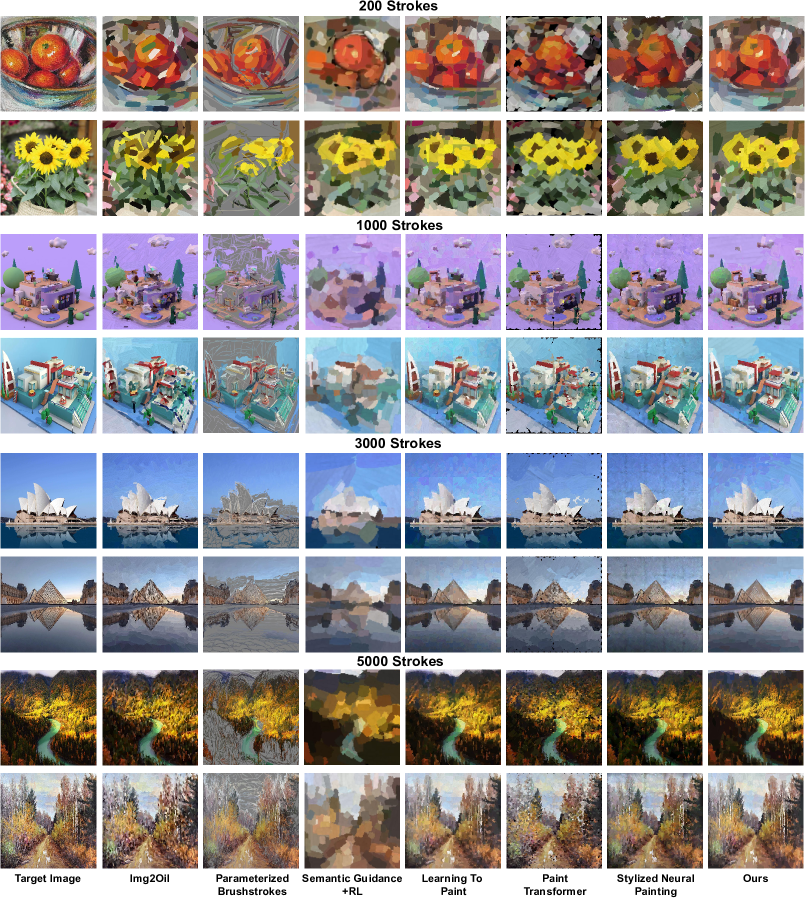
Figure 4. The comparison between our model and the state-of-the-art neural painting methods under 200, 1,000, 3,000 and 5,000 strokes. Neither Parameterized Brushstrokes  (Kotovenko et al., 2021) nor Semantic+RL  (Singh and Zheng, 2021) can reconstruct the images well. Learning To Paint  (Huang et al., 2019), Paint Transformer  (Liu et al., 2021a) and Stylized Neural Painting  (Zou et al., 2021) all suffer from the boundary inconsistency artifacts and Im2Oil  (Tong et al., 2022) has a better visual results, but lacks some details especially when the stroke number is limited (e.g., 200 strokes) In contrast, our result not only solves the boundary inconsistency problem, but also generates a better results with more details and textures. Please zoom in for more details

4. Experiments

4.1. Datasets and Settings

Datsets. We conduct experiments mainly on two datasets: CelebA-HQ(Karras et al., 2018) and ImageNet  (Deng et al., 2009). We train and test all the compared models on the two datasets separately. For each dataset, we randomly pick out 1,000 images for testing and the remaining for training.

Evaluation metrics. We evaluate the SBR results using the following three metrics:

(1) $\bm{\mathcal{L}_{2}}$ Distance calculates the mean $\mathcal{L_{2}}$ distance between the rendered images and the target images at pixel level. A lower $\mathcal{L}_{2}$ distance indicates a better image reconstruction quality.

(2) PSNR: Peak Signal to Noise Ratio (PSNR) is one of the most commonly and widely used image quality evaluation metrics. A higher PSNR indicates a better image reconstruction quality.

(3) $\bm{\mathcal{L}_{PIPS}}$  (Zhang et al., 2018) is a perceptual metric to measure the similarity between two images. A lower $\mathcal{L}_{PIPS}$ denotes a higher similarity between the rendered and target images.

4.2. Training Details

The training process consists of the three steps:

(1) Train stroke renderer. We first train our stroke renderer with synthesised data. In detail, we randomly sample stroke parameters $s$ and transform the basic stroke to get the target stroke mask $\hat{M}_{s}$. With the data pair $(s,\hat{M}_{s})$, we train our renderer by minimizing Eq.(7) for 1M iterations with batch size 32.

(2) Train painter network. After getting the stroke renderer, we train the painter network on the training dataset (CelebA-HQ or ImageNet) for 2M iterations with batch size 32.

(3) Train compositor network. With the trained painter network and renderer, we train our compositor network with the DDPG framework on the training dataset (CelebA-HQ or ImageNet) for 2M iterations with batch size 32.

Table 1. The quantitative comparison between the state-of-the-art methods and our model.

Stroke	Method	ImageNet			CelebA-HQ
Num		$\mathcal{L}_{2}$ Dist $\downarrow$	PSNR $\uparrow$	$\mathcal{L}_{PIPS}$ $\downarrow$	$\mathcal{L}_{2}$ Dist $\downarrow$	PSNR $\uparrow$	$\mathcal{L}_{PIPS}$ $\downarrow$
200	Paint Transformer (Liu et al., 2021a)	0.0585	12.86	0.1984	0.0380	14.63	0.1738
	Learning To Paint  (Huang et al., 2019)	0.0125	19.73	0.1636	0.0065	22.08	0.1578
	Semantic Guidance+RL (Singh and Zheng, 2021)	0.0191	17.67	0.1966	0.0092	20.75	0.1176
	Stylized Neural Painting (Zou et al., 2021)	0.0105	20.73	0.1625	0.0061	22.49	0.1584
	Parameterized Brushstrokes (Kotovenko et al., 2021)	0.0831	11.15	0.2259	0.0769	11.43	0.1927
	Im2oil (Tong et al., 2022)	0.0331	15.59	0.1787	0.0171	18.15	0.1822
	Ours	0.0102	20.42	0.1586	0.0044	24.01	0.1324
500	Paint Transformer (Liu et al., 2021a)	0.0379	14.80	0.1803	0.0227	16.89	0.1590
	Learning To Paint (Huang et al., 2019)	0.0092	21.13	0.1453	0.0044	23.86	0.1449
	Semantic Guidance+RL (Singh and Zheng, 2021)	0.0180	17.95	0.1970	0.0087	21.00	0.1144
	Stylized Neural Painting (Zou et al., 2021)	0.0088	21.26	0.1526	0.0046	23.65	0.1477
	Parameterized Brushstrokes (Kotovenko et al., 2021)	0.0555	13.09	0.1681	0.0725	11.71	0.1897
	Im2oil (Tong et al., 2022)	0.0263	16.89	0.1610	0.0115	19.83	0.1409
	Ours	0.0087	21.52	0.1430	0.0035	25.26	0.1202
1,000	Paint Transformer (Liu et al., 2021a)	0.0221	17.28	0.1622	0.0105	20.14	0.1443
	Learning To Paint (Huang et al., 2019)	0.0076	21.99	0.1385	0.0034	24.94	0.1327
	Semantic Guidance+RL (Singh and Zheng, 2021)	0.0171	18.16	0.1953	0.0069	22.10	0.1201
	Stylized Neural Painting (Zou et al., 2021)	0.0079	21.90	0.1458	0.0045	23.73	0.1411
	Parameterized Brushstrokes (Kotovenko et al., 2021)	0.0502	13.56	0.1524	0.0692	11.94	0.1884
	Im2oil (Tong et al., 2022)	0.0195	18.11	0.1452	0.0058	22.99	0.1506
	Ours	0.0068	22.72	0.1305	0.0024	26.62	0.1060
3,000	Paint Transformer (Liu et al., 2021a)	0.0135	19.39	0.1375	0.0067	22.16	0.1709
	Learning To Paint (Huang et al., 2019)	0.0064	22.71	0.1278	0.0029	25.72	0.1219
	Semantic Guidance+RL (Singh and Zheng, 2021)	0.0160	18.34	0.1965	0.0073	21.78	0.1201
	Stylized Neural Painting (Zou et al., 2021)	0.0100	20.62	0.1441	0.0070	21.73	0.1434
	Parameterized Brushstrokes (Kotovenko et al., 2021)	0.0437	14.18	0.1385	0.0617	12.50	0.1850
	Im2oil (Tong et al., 2022)	0.0119	20.48	0.1220	0.0029	26.07	0.1295
	Ours	0.0052	23.95	0.1106	0.0016	28.33	0.0839
5,000	Paint Transformer (Liu et al., 2021a)	0.0128	19.64	0.1353	0.0062	22.47	0.1692
	Learning To Paint (Huang et al., 2019)	0.0061	22.90	0.1255	0.0028	25.88	0.1193
	Semantic Guidance+RL (Singh and Zheng, 2021)	0.0161	18.33	0.1950	0.0075	21.84	0.1196
	Stylized Neural Painting (Zou et al., 2021)	0.0081	21.29	0.1379	0.0055	22.63	0.1667
	Parameterized Brushstrokes (Kotovenko et al., 2021)	0.0400	14.58	0.1332	0.0585	12.82	0.1847
	Im2oil (Tong et al., 2022)	0.0091	21.61	0.1118	0.0021	27.23	0.1195
	Ours	0.0046	24.57	0.1026	0.0014	28.79	0.0820

4.3. Image To Painting (Reconstruction)

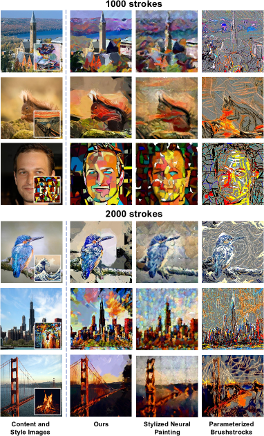
Figure 5. Stroke-based style transfer comparison with Stylized Neural Painting  (Zou et al., 2021) and Parameterized Brushstrokes  (Kotovenko et al., 2021) under 1,000 and 2,000 strokes.

Experiment Setting. The State-of-the-art model can be classified into the RL-based model (Learning To Paint  (Huang et al., 2019) and Semantic Guidance+RL  (Singh and Zheng, 2021)), the DL-based model (Paint Transformer  (Liu et al., 2021a)), the optimization-based model (Stylized Neural Painting  (Zou et al., 2021) and Parameterized Brushstrokes  (Kotovenko et al., 2021)) and the traditional search-based model (Im2Oil (Tong et al., 2022)). In this section, we compare our model to these methods (Huang et al., 2019; Singh and Zheng, 2021; Liu et al., 2021a; Kotovenko et al., 2021; Zou et al., 2021; Tong et al., 2022). For a fair comparison, we use the same oil painting brushstrokes for all the methods except Parameterized Brushstrokes since its key contribution is the specially designed renderer for Bézier stroke and follow the official implementation of all the methods. We compare the rendered results with 200, 500, 1,000, 3,000 and 5,000 strokes respectively and evaluate the results both qualitatively and quantitatively.

Among the existing methods, Learning To Paint (Huang et al., 2019) is the pioneering model capable of accurately reconstructing most of the details in the input image. Building on it, Semantic Guidance+RL (Singh and Zheng, 2021) incorporates semantic guidance into the RL training process, enabling the model to focus more on the semantic part. To overcome the challenges posed by the long training time and unstable agent of the RL method, Paint Transformer (Liu et al., 2021a) proposes a RL-free model. However, the painter network in Paint Transformer only reconstructs images at a coarse level and requires much more strokes than the RL-based models for the same image. Additionally, both Stylized Neural Painting and Parameterized Brushstrokes render images through the optimization process, which suffers from a long optimization time for each individual image. Among all these methods, Im2Oil (Tong et al., 2022) is the only approach that adopts the traditional greedy-search strategy, which also entails considerable search time.

Figure 4 shows the rendered images by Learning To Paint, Semantic Guidance+RL, Paint Transformer, Stylized Neural Painting and Parameterized Brushstrokes and Im2Oil. It can be seen that all the results generated by the uniform-block-dividing strategy (Learning To Paint, Paint Transformer and Stylized Neural Painting) have the boundary inconsistency problem. Moreover, the Semantic Guidance+RL method cannot use the uniform-block-dividing strategy so that it fails to reconstruct the details in a complex real image. Im2Oil has a relatively good visual quality, but lacks some details especially when the stroke number is limited (e.g., 200 strokes). In contrast, our model not only solves the boundary inconsistency artifacts, but also render the images with the richest details. We also conduct a quantitative comparison between our model and the state-of-the-art methods. We evaluate the average $L_{2}$ distance, PSNR and $\mathcal{L}_{PIPS}$ between 1,000 target images and the generated images among these methods in Table 1 (100 images for Stylized Neural Painting, Parameterized Brushstrokes and Im2Oil due to their slow optimization process) . It shows that our model outperforms all the state-of-the-art methods in most of the conditions.

4.4. Stroke-based Style Transfer

We compare our model with the state-of-the-art stroke-based style transfer methods Stylized Neural Painting (Zou et al., 2021) and Parameterized Brushstrokes (Kotovenko et al., 2021) using the same number of strokes (1,000 and 2,000) and their default stylization settings. The results in Fig. 5 demonstrate that Stylized Neural Painting suffers from severe boundary artifacts, while Parameterized Brushstrokes fails to maintain most of the contents. Furthermore, both methods lose a significant amount of information in the object boundaries, resulting in blurred edges and structures in the generated images. (Note that Parameterized Brushstrokes (Kotovenko et al., 2021) can achieve relatively good stylization results with a large amount stroke count (over 10,000) as shown in their paper) In contrast, our model not only preserves the structure of content images well, but also delivers superior stylization effects and visual quality when compared to the aforementioned methods. Furthermore, we quantitatively compare the stylization effects of each method by computing the distance between the gram matrices of the generated images and style images in Fig. 5 as a measurement of stylization effectiveness. The results explicitly show that our method has a significantly improved average distance of 0.6943 compared to Stylized Neural Painting (1.4048) and Parameterized Brushstrokes (4.0274), indicating that our model has a superior stylization performance.

4.5. Ablation Study

Ablation study on the compositor network. In this part, we validate the importance of our compositor network and the function of our phasic reward mechanism. We train 3 ablated models: (1) a model without the compositor network (only a painter network and a stroke renderer); (2) a model without the compositor network but using the uniform-block-dividing strategy; (3) an ablated model without the phasic reward. Tab. 2 and Fig. 6 show the comparison results. It can be seen that the model without the compositor network or phasic reward fails to reconstruct image details and the model with uniform-block-dividing strategy suffers from the boundary artifacts (Fig. 6(c)).

Table 2. Ablation Study on the compositor and painter network on the ImageNet dataset.

Method		1,000 Strokes			5,000 Strokes
Compositor	Painter	$\mathcal{L}_{2}$ Dist $\downarrow$	PSNR $\uparrow$	LPIPS $\downarrow$	$\mathcal{L}_{2}$ Dist $\downarrow$	PSNR $\uparrow$	LPIPS $\downarrow$
no compositor	our painter	0.0122	19.88	0.1739	0.0134	19.45	0.1705
w/o phasic reward	our painter	0.0099	20.31	0.1389	0.0098	20.83	0.1364
block division	our painter	0.0071	22.32	0.1345	0.0058	23.12	0.1194
our compositor	w/o $\mathcal{L}_{adv}$	0.0241	16.62	0.1766	0.0239	16.65	0.1762
our compositor	w/o adaptive regularization	0.0129	19.47	0.1689	0.0109	20.20	0.1558
our compositor	noise as real sample	0.0072	22.35	0.1325	0.0049	24.02	0.1047
our compositor	our painter	0.0068	22.72	0.1305	0.0046	24.54	0.1026

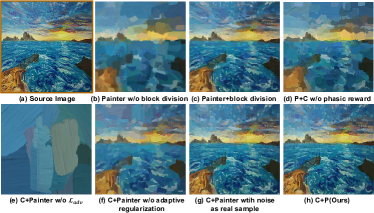
Figure 6. Ablation Study on the compositor (C) and painter network (P). The model without compositor either fails to reconstruct the details (b) or suffers from the boundary artifacts (c). The model without phasic reward reconstructs less details (d) than the standard model (h). As for the painter network, the model without $\mathcal{L}_{adv}$ (e) tends paint the same big strokes repeatedly. And the model without the adaptive regularization factor $\gamma$ (f) fails to paint the image details. The model taking random noise as the real WGAN sample (g) has a similar results to the standard model (h).

Ablation study on the painter network. To validate the effectiveness of the key components of our painter network, we train 3 ablated models: one model without the adversarial loss $\mathcal{L}_{adv}$, one model without the adaptive regularization factor $\gamma$, and one model with random noises being the real samples. We employ both the compositor and painter network to conduct the experiments and the results are shown in Tab. 2 and Fig. 6. It can be seen that the model without $\mathcal{L}_{adv}$ tends to paint the same big strokes repeatedly. And the model without $\gamma$ suffers from an unstable training process, resulting in a worse painting performance than our model. Moreover, with random noises being the real samples, the model can also achieve a similar performance as our baseline model, indicating that penalizing seen fake samples to avoid painting similar strokes is the main function of our discriminator $D$.

5. Conclusion

In this paper, we propose Compositional Neural Painter, a novel stroke-based rendering framework which dynamically predicts the next painting region based on the current canvas, instead of dividing the image plane uniformly into $K\times K$ painting regions. Moreover, we extend our method to edge-promoting stroke-based style transfer task with a novel differentiable distance transform loss. Extensive quantitative and qualitative experiments show that our model outperforms the state-of-the-art methods in both stroke-based neural rendering and stroke-based stylization.

Appendix A Overview

This appendix consists of:

1) The training details of our model (Sec. B);

2) Ablation study on our distance transform loss (Sec. C);

3) Visualization of the painting process of our model (Sec. D);

4) User study on the painting performance (Sec. E);

5) Comparison between the painter networks of our model and the existing methods (Sec. F);

6) Comparison with the local attention window proposed in Intelli-Paint (Singh et al., 2022) (Sec. G);

7) More comparison results with the existing methods on stroke-based painting (Sec. H);

8) More comparison results on Stylization which includes the stylization method in pixel level (Sec. I);

9) The time complexity analysis on each method (Sec. J).

Appendix B Training Details

The training process consists of three steps:

(1) Train stroke renderer. We first train our stroke renderer with synthesized data. In detail, we randomly sample stroke parameters $s$ and transform the basic stroke to get the target stroke mask $\hat{M}_{s}$. With the data pair $(s,\hat{M}_{s})$, we train our renderer by minimizing Eq.(7) in the main paper for 1M iterations with batch size 32.

(2) Train painter network. After getting the stroke renderer, we train the painter network on the training dataset (CelebA-HQ or ImageNet) for 2M iterations with batch size 32.

(3) Train compositor network. With the trained painter network and renderer, we train our compositor network with the DDPG framework on the training dataset (CelebA-HQ or ImageNet) for 2M iterations with batch size 32.

Appendix C Ablation study on DT loss

In this section, we perform an ablation study on the distance transform (DT) loss of our stroke-based stylization method in order to assess its efficacy. We conducted a comparative experiment between our stroke-based stylization model (with DT loss) and the DT loss-free model as demonstrated in Fig. 7. It can be observed that in the first row of the figure, the DT loss-free model loses a significant amount of edge information in regions with comparatively blurred edges. Moreover, in the second row of the figure, the DT loss-free model exhibits edge disturbances specifically along straight edges (i.e., building outlines). In contrast, our model incorporating DT loss maintains the structure of the content image effectively in both the situations (blurred edges and straight edges).

Appendix D Painitng Process

In this section, we visualize the painting process of our model, as shown in Fig. 8. We present the images generated by the model at various stages of painting, corresponding to 5, 100, 500, 2000, and 5000 brush strokes, respectively. It can be observed that our model initially tends to capture the overall background contours of the image during the early stages of painting. Subsequently, it gradually enriches the image with finer details. As the number of brush strokes increases, the model’s capability to reconstruct intricate details strengthens, ultimately yielding satisfying results in the final painting.

Appendix E User study

To further validate the effectiveness of our model, we invite 30 volunteers to rank the generated results of our approach, Learning To Paint (Huang et al., 2019), Paint Transformer (Liu et al., 2021a), Stylized Neural Painting (Zou et al., 2021) and Im2Oil (Tong et al., 2022), based on their perceived quality from best to worst. The results are presented in Tab. 3. It can be seen that our model gets the top rank in 65% of the cases. Furthermore, our average ranking stands at an impressive 1.56, indicating superior performance compared to the other methods.

Appendix F Comparison between the painter networks

The existing painter networks can be divided into two types: one that utilizes reinforcement learning (Learning To Paint  (Huang et al., 2019), Semantic Guidance+RL (Singh and Zheng, 2021), etc), and the other that does not (Paint Transformer (Liu et al., 2021a)). (a) Compared to Painter Transformer that does not employ reinforcement learning, our approach trains the network using real data rather than synthetic data, and incorporates adversarial learning to enhance the exploration capability, resulting in significantly improved painting performance. (b) Compared to reinforcement learning-based methods, our approach adopts deep learning training strategy, which has a simpler training framework and yields a stabler training process, while achieving better stroke-based painting results.

To validate this, we compare the painter networks of Learning To Paint, Paint Transformer, Semantic Guidance+RL and ours without block division on ImageNet (Deng et al., 2009) and CelebA-HQ datasets (Karras et al., 2018) (200 strokes) in Tab.  4. It can be seen that our painter network exhibits the lowest $\mathcal{L}_{2}$ distance and LPIPS score, as well as the highest PSNR, indicating its superior image reconstruction capability over all other models.

Appendix G Comparison with Intelli-Paint

In Intelli-Paint (Singh et al., 2022), the concept of attention window is proposed. Initially, Intelli-Paint employs object detection method on the input image to derive a global attention window. Using this global attention window, a neural network is trained to simultaneously predict both the local attention window and stroke parameters. Subsequently, the stroke parameters are mapped onto the local attention window for painting, which is reminiscent of our dynamic painting region strategy. Nevertheless, the motivation, usage of attention window, and resulting painting effects between Intelli-Paint and our model are significantly different.

From a motivation perspective, Intelli-Paint uses the attention window to simulate the painting process of human artists, where the $i$th stroke and $i+1$th stroke are typically drawn close to each other in the canvas. They constantly slide the attention window, which enables the model to paint anywhere in the detected object window. In contrast, our goal is to utilize the painting region (can be regarded as a type of attention window) to enable the painter network to focus solely on the local details of the image, which leads to better reconstruction of image details.

Table 3. User study results summarized from rankings of 30 participants. Our model ranks first in 65% cases with an average ranking of 1.56.

Method	Ours	Learning To Paint	Paint Transformer	Stylized Neural Painting	Img2Oil
Percentage of ranking first (%)$\uparrow$	65.00%	14.89%	5.78%	9.56%	4.78%
Average ranking$\downarrow$	1.56	2.54	3.55	3.18	4.15

Table 4. Comparison between the painter networks of Learning To Paint (Huang et al., 2019), Semantice Guidance+RL (Singh and Zheng, 2021), Paint Transformer (Liu et al., 2021a) and ours on ImageNet (Deng et al., 2009) and Celeba-HQ (Karras et al., 2018) dataset with 200 strokes. It can be seen that our painter network outperforms the other ones in stroke-based rendering.

Method	ImageNet			CelebA-HQ
	$\mathcal{L}_{2}$ Dist $\downarrow$	PSNR $\uparrow$	LPIPS $\downarrow$	$\mathcal{L}_{2}$ Dist $\downarrow$	PSNR $\uparrow$	LPIPS $\downarrow$
Learning To Paint	0.0160	18.48	0.1871	0.0082	21.17	0.1388
Semantic Guidance+RL	0.0197	17.65	0.2101	0.0092	20.75	0.1176
Paint Transformer	0.1497	8.54	0.2180	0.1127	10.06	0.2045
Our Painter	0.0108	20.12	0.1639	0.0064	22.19	0.1299

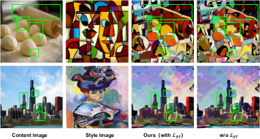
Figure 7. Ablation study on distance transform loss in stroke-based stylization. The model without DT loss loses some structure information (shown in the green boxes). In contrast, our model with the DT loss preserves the structures well.

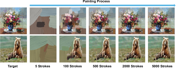
Figure 8. The Painting process of our model. Our model initiates the painting process by capturing the overall structure of the entire image and subsequently enriches the artwork with finer details. As the number of brush strokes increases, the painting results become increasingly intricate and refined.

In terms of usage, Intelli-Paint employs a single network to simultaneously predict both the attention window and stroke parameters, which poses a significant burden on the RL-based neural painting model. Similar to Learning To Paint (Huang et al., 2019), the network in Intelli-Paint finds it challenging to predict a long sequence of stroke parameters, such as those exceeding 2,000 strokes. In contrast, our approach separates the prediction of the painting region and stroke parameters into two distinct stages, which are trained separately by combining the compositor network and the painter network. This two-stage training and testing strategy effectively enhances the number of strokes in the painting process.

Finally, in terms of resulting effects, Intelli-Paint focuses on painting images with clear objects and has difficulty reconstructing satisfactory details for images without clear objects, such as landscapes, due to limitations in its network design (one network predicts both the attention window and stroke parameters at the same time). In contrast, our model can paint images with fine-grained details in any situation. As Intelli-paint’s code is not open-sourced, we replicate their attention window design based on Learning To Paint (Huang et al., 2019) since both of them are trained with DDPG and demonstrate that their attention window design could not achieve accurate reconstruction of image details but only mimic the human painting style, namely, the close proximity between two consecutive brushstrokes. The comparison results are shown in Fig. 9.

In order to further validate our model’s ability to capture more intricate details than Intelli-Paint without the need for object detection, we select several images from the best-performing examples in the paper of Intelli-Paint. We then employ our model to perform painting on these images and compared the results. As illustrated in Figure  10, our model achieved noticeably superior painting results, reconstructing much more intricate image details than Intelli-Paint.

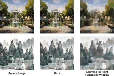
Figure 9. The comparison between our methods and the reproduction of attention window in Intelli-Paint. It shows that the attention window in Intelli-Paint can not reconstruct the image details.

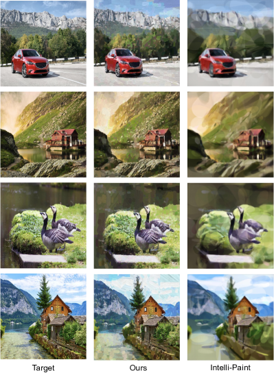
Figure 10. The comparison between our results and the best-painted images shown in the paper of Intelli-Paint. Our model can reconstruct much more intricate details than Intelli-paint.

Appendix H More Comparison on Stroke-based Painting

H.1. More comparison on oil brushstrokes

In Section 4.3 of the main paper, we compare our model with the state-of-the-art stroke-based painting methods (Huang et al., 2019; Liu et al., 2021a; Zou et al., 2021; Kotovenko et al., 2021; Singh and Zheng, 2021; Tong et al., 2022). In this section, to further validate our model’s ability in stroke-based neural painting, we show more comparison results.

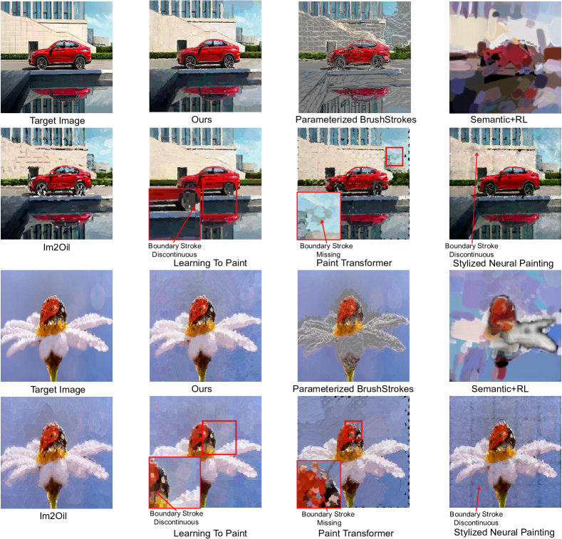
Figure 11. More comparison results to the existing methods (3,000 strokes). The methods which employ the uniform-block-dividing strategy (Learning To Paint, Paint Transformer and Stylized Neural Painting) all suffer from the boundary inconsistency artifacts. Please zoom in for details.

In Fig. 11, all methods use 3,000 strokes to paint the images. Parameterized Brushstrokes (Kotovenko et al., 2021) and Semantic + RL (Singh and Zheng, 2021) fail to reconstruct most of the details in the target image. Note that RL+Semantic requires the prediction of semantic region, and when the semantic region is wrongly predicted (the second and third examples in Fig. 11), its results lose most of the information in the target image. In contrast, our method reconstructs the target images better under the same number of strokes.

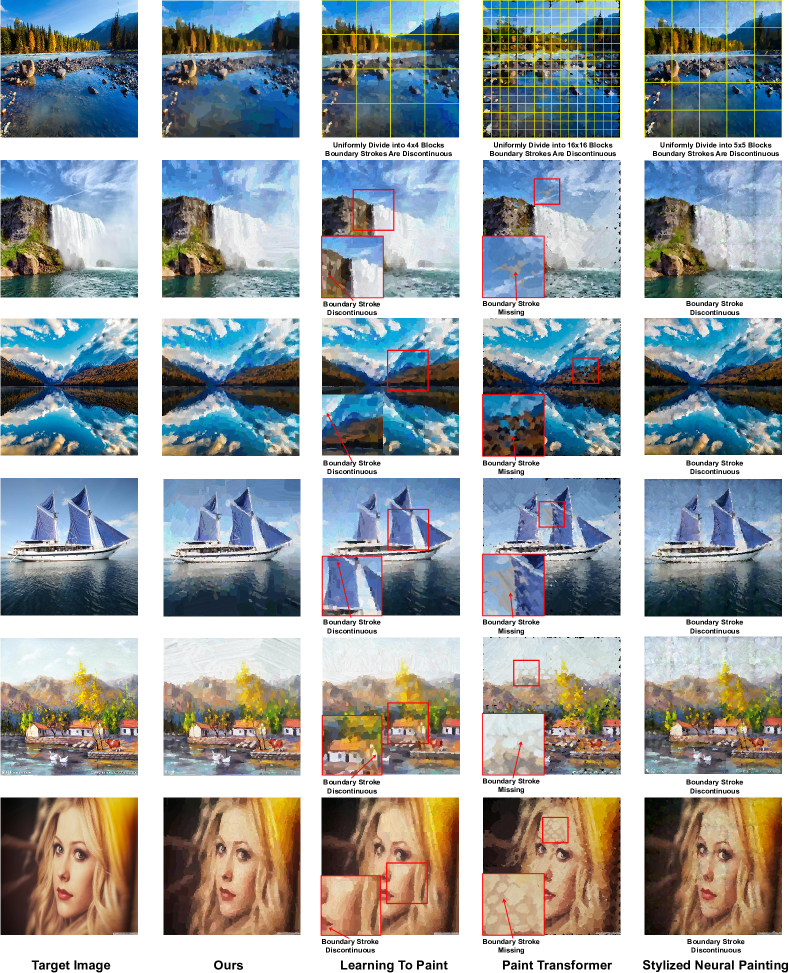
Figure 12. More comparison results (5,000 strokes) with the methods which employ the uniform-block-dividing strategy. All the compared methods (Learning To Paint, Paint Transformer and Stylized Neural Painting) suffer from the boundary inconsistency artifacts while our model is free from the boundary inconsistency artifacts and has a better reconstruction quality.

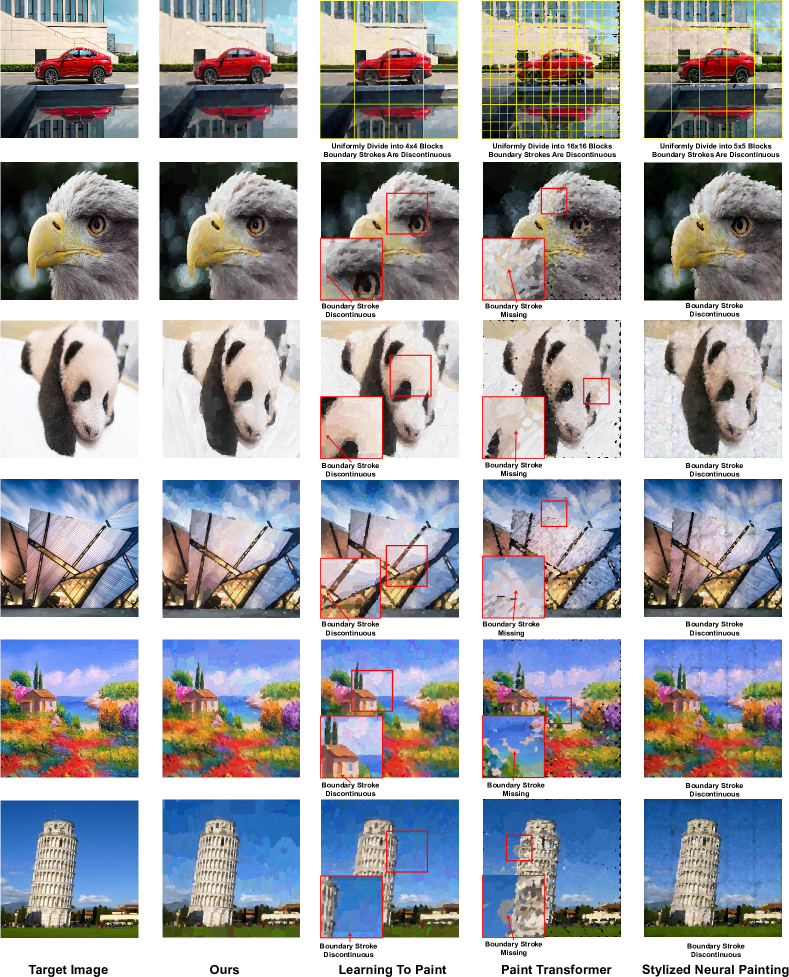
Figure 13. More comparison results (5,000 strokes) with the methods which employ the uniform-block-dividing strategy. All the compared methods (Learning To Paint, Paint Transformer and Stylized Neural Painting) suffer from the boundary inconsistency artifacts while our model is free from the boundary inconsistency artifacts and has a better reconstruction quality.

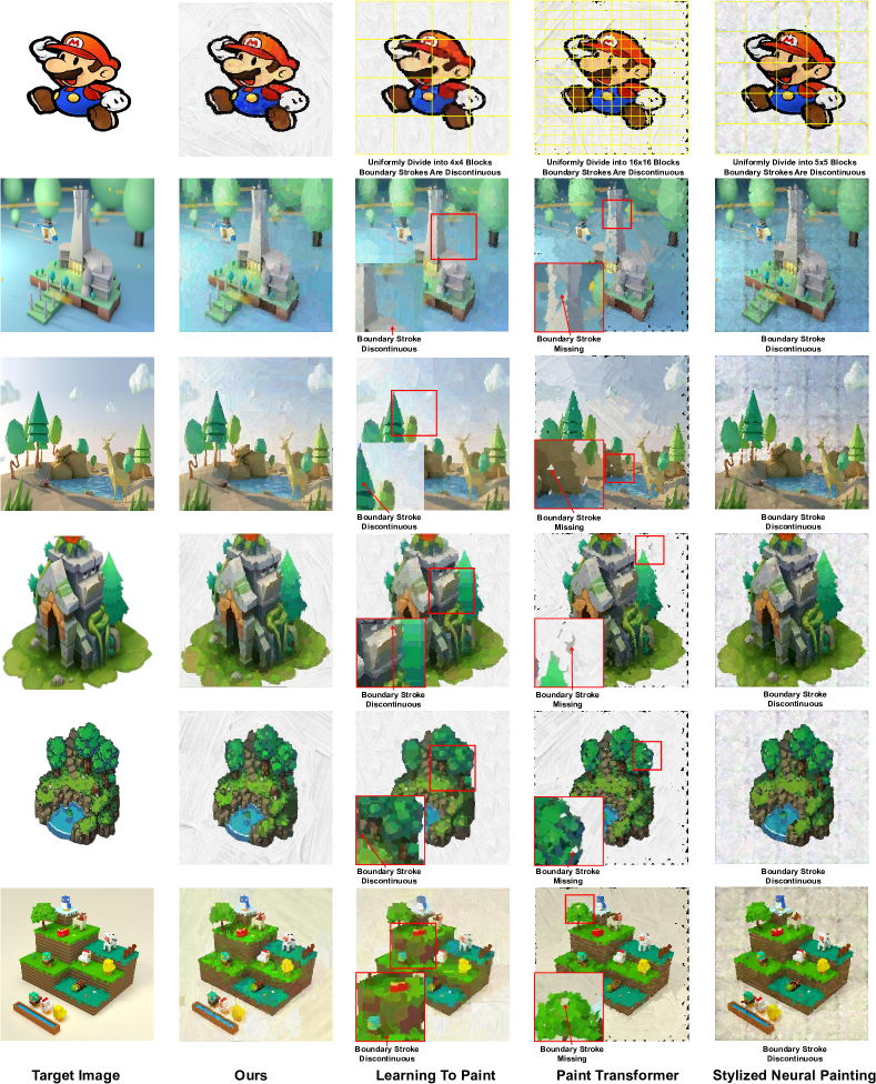
Figure 14. More comparison results (5,000 strokes) with the methods which employ the uniform-block-dividing strategy. All the compared methods (Learning To Paint, Paint Transformer and Stylized Neural Painting) suffer from the boundary inconsistency artifacts while our model is free from the boundary inconsistency artifacts and has a better reconstruction quality.

Learning To Paint (Huang et al., 2019), Paint Transformer (Liu et al., 2021a) and Stylized Neural Painting (Zou et al., 2021) are three comparison methods that utilize the uniform-block-dividing strategy, i.e., dividing the image plane uniformly into blocks, and then predicting strokes for each block independently, which enables a better reconstruction performance. However, they suffer from the boundary inconsistency artifacts: as shown in Fig. 11 and more examples in Figs. 12-14 (5,000 strokes), there are obvious discontinuous strokes on the two sides of the block boundaries. In contrast, with dynamically predicted painting regions, our model is free from the boundary inconsistency artifacts and paints the target images with the most details.

H.2. Comparison with transparent brushstrokes

In Learning To Paint (Huang et al., 2019), it employs transparent brushstrokes constructed by a large number of circles of different sizes to paint the images. It differs from real oil brushstrokes in terms of transparency and stroke texture. But to show the effectiveness of our method, we still compare with the state-of-the-art methods (Learning To Paint (Huang et al., 2019) and Semantic Guidance+RL(Singh and Zheng, 2021)) which uses transparent brushstrokes in their default settings. In this experiment, we employ transparent burshstroke to train our model and compare it with the given model from their official links. We use $\mathcal{L}_{2}$ distance, PSNR and LPIPS as the comparison metric and paint 1,000 images in both ImageNet  (Deng et al., 2009) and CelebA-HQ(Karras et al., 2018) dataset. The quantitative comparison results are shown in Tab. 5. It can be seen that our method outperforms both Learning To Paint and Semantic Guidance+RL with their transparent brushstrokes, indicating that our model has the same superior performance and strong robustness under different kinds of brushstrokes. Note that when painting images in CelebA-HQ dataset with 5,000 strokes, due to the simple structure and few details in human faces, our model performs similarly to Learning To Pain. But when the images become more complex (i.e., images in ImageNet), our model surpasses Learning To Paint in terms of both the reconstruction ability and perceptual similarity.

Table 5. The quantitative comparison between the state-of-the-art methods and our model with the original transparent brushstrokes in Learning To Paint.

Stroke	Method	ImageNet			Celeba-HQ
Num		$\mathcal{L}_{2}$ Dist $\downarrow$	PSNR $\uparrow$	LPIPS $\downarrow$	$\mathcal{L}_{2}$ Dist $\downarrow$	PSNR $\uparrow$	LPIPS $\downarrow$
200	Learning To Paint  (Huang et al., 2019)	0.0126	19.72	0.1658	0.0087	20.84	0.1534
	Semantic Guidance+RL (Singh and Zheng, 2021)	0.0126	19.61	0.2034	0.0084	20.97	0.1829
	Ours	0.0073	22.07	0.1593	0.0039	24.31	0.1307
500	Learning To Paint  (Huang et al., 2019)	0.0082	21.81	0.1398	0.0032	25.36	0.1098
	Semantic Guidance+RL (Singh and Zheng, 2021)	0.0118	19.90	0.2019	0.0076	21.46	0.1818
	Ours	0.0060	23.29	0.1417	0.0025	26.37	0.1034
1,000	Learning To Paint  (Huang et al., 2019)	0.0058	23.49	0.1179	0.0020	27.44	0.0853
	Semantic Guidance+RL (Singh and Zheng, 2021)	0.0117	19.97	0.2028	0.0073	21.65	0.1786
	Ours	0.0047	24.59	0.1154	0.0018	27.80	0.0850
3,000	Learning To Paint  (Huang et al., 2019)	0.0039	25.31	0.0975	0.0013	29.23	0.0670
	Semantic Guidance+RL (Singh and Zheng, 2021)	0.0117	19.99	0.2030	0.0076	21.50	0.1802
	Ours	0.0033	25.99	0.0956	0.0013	29.24	0.0667
5,000	Learning To Paint  (Huang et al., 2019)	0.0036	25.71	0.0943	0.0012	29.49	0.0658
	Semantic Guidance+RL (Singh and Zheng, 2021)	0.0116	20.03	0.2031	0.0073	21.69	0.1791
	Ours	0.0030	26.35	0.0905	0.0012	29.49	0.0637

Appendix I More Stroke-based Stylization Experiments

In Section 4.4 of the main paper, we compare our model with the state-of-the-art stroke-based stylization methods: Stylized Neural Painting (Zou et al., 2021) and Parameterized Brushstrokes (Kotovenko et al., 2021). In this section, we take the stylization methods in pixel level into consideration and compare with them.

We compare our stroke-based stylization model with the existing methods, including stroke-based stylization methods: Stylized Neural Painting (Zou et al., 2021) and Parameterized Brushstrokes (Kotovenko et al., 2021), and pixel-based stylization methods: Gatys (Gatys et al., 2016), AdaIN (Huang and Belongie, 2017) and AdaAttN (Liu et al., 2021b). We use the default stroke number for the stroke-based methods: 2,000 strokes for Stylized Neural Painting and Ours, and 10,000+ strokes for Parameterized Brushstrokes. We employ the official implementations from Github for all the comparison methods to conduct this experiment.

The comparison results are shown in Fig. 15. Compared to the stroke-based stylization methods (Stylized Neural Painting and Parameterized Brushstrokes), our model better preserves semantic contents in the content images and has a better visual quality. And our stroke-based model achieves stylization results as good as pixel-based methods (Gatys, AdaIN and AdaAttN).

Appendix J Time Complexity Analysis

To have a more comprehensive comparison, we further compare the inference time of each method on a single 24G RTX3090 GPU. Specifically, we set the stroke number to be 1,000 and we randomly select 100 images from the Celeba-HQ dataset to test the inference time. For each method, we use the default settings from the official code and only count the model’s running time (i.e., ignore the loading and storage time). We average the inference time for the selected 100 images and report it in Tab. 6. We can see that Learning to Paint has the fastest inference speed (0.2066s) while our model follows closely behind (0.2162s), indicating that our model has both a good painting performance and efficiency.

Table 6. Comparison on the average inference time.

Model	Ours	Learning To Paint	Semantic +RL	Paint Transformer
Inference Time	0.2162s	0.2066s	2.9921s	0.3725s
Model	Im2Oil	Stylized Neural Painting	Parameterized Brushstrokes
Inference Time	55.3714s	124.9371s	247.6105s

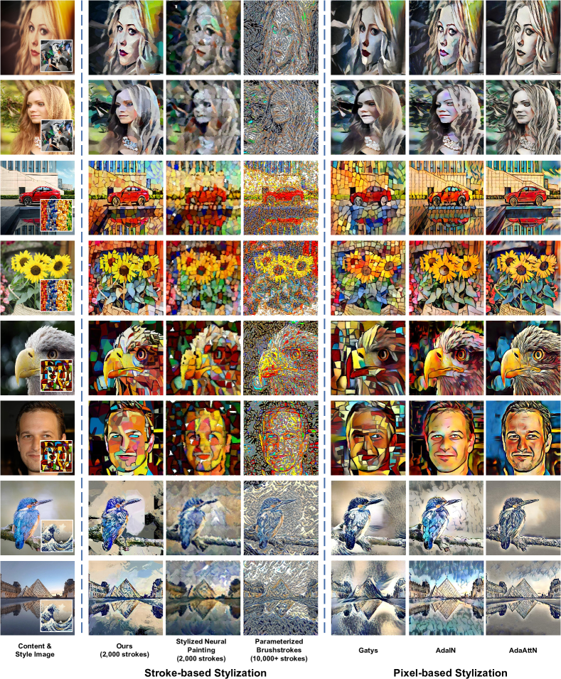
Figure 15. Stylization comparison with the existing methods. Compared to the stroke-based stylization methods (Stylized Neural Painting and Parameterized Brushstrokes), our model better preserves semantic contents in the content images and has a better visual quality. And our stroke-based model achieves stylization results as good as pixel-based methods (Gatys, AdaIN and AdaAttN).