Phase Transition and Subshifts of Finite Type

Abstract

The aim of this article is to establish freezing phase transition of the pressure function, considering the generalized Hofbauer potential $\varphi$, which is connected to the distance from subshift of finite type $\Sigma_{\mathcal{F}}$ in the full shift $\Sigma$ over finite alphabets. Our objective is to prove that the pressure function exhibits phase transition with the dominating measure is highly concentrated on $\Sigma_{\mathcal{F}}$ after the transition. Moreover, the pressure function attains $C^{1}$-smoothness when the transition occurs at 2.

AMS classification: 37D35, 82B26, 37A60, 37B10, 68R15.

Keywords: thermodynamic formalism, freezing phase transition, subshift of finite type, equilibrium states.

1 Introduction

Thermodynamic formalism originated as a branch of statistical physics and underwent a transformation into a mathematical discipline during the 1970s, especially due to the work of Ruelle, Sinai, and Bowen [2, 18, 22]. In this framework, consider a dynamical system $(X,T)$ and a continuous function $\varphi:X\rightarrow{\mathbb{R}}$, referred to as the potential. The pressure function [23] associated with the system $(X,T)$ is defined as follows:

$${\mathcal{P}}(\beta)=\sup_{\mu\in{\mathcal{M}}_{T}(X)}\Big{\{}h_{\mu}+\beta\int\varphi d\mu\Big{\}},$$ (1)

Here, $\mu$ ranges over the space ${\mathcal{M}}_{T}(X)$ consisting of all $T$-invariant probability measures on $X$, $h_{\mu}$ represents the entropy of the measure $\mu$ [24], and $\beta$ is a real parameter. An invariant probability measure $\mu$ that achieves the supremum in equation (1) is termed an equilibrium measure of the system $(X,T,\beta\varphi)$.

Bowen’s work [2] established significant results concerning the analytic properties of dynamical pressure. Additionally, it demonstrated the absence of phase transitions for potentials that satisfy Hölder continuity conditions in the setting of hyperbolic dynamical systems. These findings were particularly relevant in the context of hyperbolic dynamical systems, with shift of finite type serving as an essential subclass.

Specifically, systems known as shifts of finite type emerged as a significant subclass within hyperbolic dynamical systems. While symbolic dynamical systems may seem somewhat abstract from a physical perspective, they have proven to be a fertile ground for extending Bowen’s findings. These systems, where spaces are composed of sequences of symbols, provide a valuable framework for further expanding upon the outcomes of Bowen’s work.

Hafbauer [7] demonstrated that in the setting of the binary full shift, a phase transition can arise when considering a non-Hölder (Hofbauer) potential. Specifically, for the Hafbauer potential, the nature of the potential at a given point $x$ is intricately linked to the distance between $x$ and the constant sequence $0^{\infty}$. In this scenario, it becomes feasible to perform explicit calculations, revealing that the family of potentials exhibits a phase transition. This transition is marked by a discontinuous change in the equilibrium measure. Importantly, this phase transition assumes a freezing nature; as $\beta$ becomes large ($\beta\rightarrow\infty$), the sole measure that attains maximal pressure is the Dirac delta at $0^{\infty}.$

Several years back, H. Bruin and R. Leplaideur [5, 4] introduced a challenging question involving potentials linked to the proximity of a subshift, giving rise to what is now referred to as the ”generalized Hofbauer potential.” Bruin and Leplaideur subsequently tackled this question, obtaining outcomes for subshifts corresponding to classical one-dimensional quasi fractals, specifically those linked to Thue-Morse and Fibonacci Sturmian sequences. However, when considering this matter in its complete generality, the problem remains wide open and deeply captivating. In their work, Bruin and Leplaideur assert that a freezing phase transition arises when the parameter $\beta$ is sufficiently large. Additionally, they established that the equilibrium measure, following this freezing phase transition, finds its support on a non-trivial quasi fractal subset of the binary full shift. In a related endeavor [12], an estimate for the transition point was achieved in line with the outcomes of [5]. Nonetheless, results of this nature were not previously established for subshifts of finite type.

This article focus into the investigation of phase transition outcomes concerning the generalized Hofbauer potential, which derives its values from the mixing subshift of finite type. The objective is to establish the occurrence of a phase transition within these systems and to demonstrate the alignment between the pressure function’s value and the entropy of the respective subshift. Notably, following this transition, the equilibrium measure becomes strongly concentrated on the specific targeted subshift. It’s worth noting that the theory of thermodynamic formalism exhibits striking parallels between the case of subshifts of finite type and the concept of the Hofbauer potential.

The article is structured in the following manner:

In Section 2, we delve into the fundamental tools of combinatorics on words that are closely tied to symbolic dynamics. These tools will serve as a foundation for our analysis throughout the article. Additionally, towards the conclusion of this section, we will outline key components of thermodynamic formalism within the context of a one-sided full shift.

Section 3 of the paper establishes the context of our study. This involves defining our system and introducing the potential function $\varphi$. In a related work [13], R. Leplaideur introduced a powerful approach referred to as the ”Inducing Scheme,” which is instrumental in identifying multiple equilibrium states of the system, should they exist. This approach will allow us to specify our core theorem, where we focus on the spectral radius of the induced transfer operator, tailored to our specific configuration. Additionally, under this framework, we will then present our primary theorem within the established context.

The concluding section, Section 4, is devoted to the proof of our main theorem. The initial segment of this section is focused on utilizing the nature of spectral radius through inducing scheme [13], to identify the occurrence of a phase transition. Subsequently, we delve into a discussion regarding the smoothness properties of the pressure function at the transition parameter. Lastly, we present illustrative examples to underscore our findings and draw a comparative analysis with the Hofbauer case.

2 Basic Definitions and Examples

In this section, our aim is to lay down the fundamental concepts essential for understanding the core theme of article. The primary focus will be on introducing key terminologies from combinatorics on words and symbolic dynamical systems. For further detail on this section, we direct the readers to references [16, 17].

2.1 Word Combinatorics

Let ${\mathcal{S}}=\{0,1\cdots m-1\}$ be the set of finite alphabets. These elements within ${\mathcal{S}}$ can be referred to as letters, states or symbols. A finite word is essentially finite sequence of symbols. If $u=u_{0}u_{1}\cdots u_{p-1}$ be a finite word, the value $p$ signifies the length of $u$, denoted by $|u|$. We denote $\epsilon$ is the empty word, the sole word with a length is zero. The concatenation of words $u=u_{0}u_{1}\cdots u_{p-1}$ and $v=v_{0}v_{1}\cdots v_{q-1}$ is the word $uv=u_{0}u_{1}\cdots u_{p-1}v_{0}v_{1}\cdots v_{q-1}.$ We denote $\Sigma^{+}$ is the set of all finite words over ${\mathcal{S}}$.

A finite word $u=u_{0}u_{1}\cdots u_{p-1}$ is called a factor of another word $v$ if there exist words $r,s\in\Sigma^{+}$ such that $v=rus$. The word $u$ is called (i) a prefix of $v$ if $r=\epsilon$, (ii) a suffix of $v$ if $s=\epsilon$, (iii)an inner factor of $v$ if $r\not=\epsilon$ and $s\not=\epsilon$.

A (one-sided) infinite word is an infinite sequence over ${\mathcal{S}}$; we denote this as

$$z=z_{0}z_{1}z_{2}\cdots z_{p-1}\cdots,$$

where $z_{i}\in{\mathcal{S}}$ for all $i\in{\mathbb{N}}$, signifying an infinite word. The set $\Sigma={\mathcal{S}}^{{\mathbb{N}}}$ is the set of all (one-sided) infinite words over set ${\mathcal{S}}$.

The notions of prefix, factor and suffix introduced to finite words can be naturally extended to infinite word. While an infinite word’s factors and prefixes remain finite, but a suffix of an infinite word is an infinite word. Given $z\in\Sigma$, then the language of $z$ is the set of all its factors set is denoted by $L(z)$. For $n\geq 1$, the set $L_{n}(z)=\left\{u\in L(z):|u|=n\right\}$ is the set of factors of length $n$ occurring in $z$.

2.1.1 Symbolic Dynamics

We remind that the set $\Sigma$ is the set of all infinite words derived from ${\mathcal{S}}$. Given two infinite words $x=x_{0}x_{1}x_{2}\cdots$ and $y=y_{0}y_{1}y_{2}\cdots$, their distance is determined by $2^{-k(x,y)}$, where

$$k(x,y)=\min\left\{k\in{\mathbb{N}}\cup\{+\infty\}:x_{k}\not=y_{k}\right\}.$$

The formulation holds with the understanding that $d(x,y)=0$ when $x=y$. This distance metric defines a topology on the set $\Sigma$, rendering space $\Sigma$ a complete, compact Cantor set.

For any $x\in\Sigma$, the shift is the function $\sigma:\Sigma\rightarrow\Sigma$ defined by

$$\sigma(x_{0}x_{1}x_{2}\cdots)=x_{1}x_{2}x_{3}\cdots.$$

The map $\sigma$ is uniformly continuous, onto, but not a one-to-one function on $\Sigma$. The dynamical system $(\Sigma,\sigma)$ is known as (one-sided) full shift over the set ${\mathcal{S}}$.

Considering a finite word $u=u_{0}u_{1}\cdots u_{n-1}$, the associated cylinder set $[u]$ is precisely defined by:

$$[u]=\left\{y\in\Sigma:y_{i}=u_{i}\,,\,\,\forall\,\,\,0\leq i\leq n-1\right\}.$$

These cylinder sets are clopen sets within $\Sigma$. In addition, the entire collection of cylinder sets constructs a basis for the full shift $\Sigma$.

A subset of the full shift $\Sigma$, which is both invariant and closed under the shift map, is termed a subshift or a Symbolic Dynamical system. Below is the definition for the subshift of finite type.

Definition 2.1.

Let ${\mathcal{F}}$ be a finite subset of $\Sigma^{+}$. The set

$$\Sigma_{{}_{\mathcal{F}}}=\left\{z\in\Sigma_{{}_{\mathcal{S}}}:L(z)\cap{\mathcal{F}}=\epsilon\right\},$$

i.e., The subset of $\Sigma$, whose elements avoid ${\mathcal{F}}$ factors, forms a subshift of $\Sigma$ is called subshift of finite type.

The language of a subshift of finite type is denoted by $L(\Sigma_{{}_{\mathcal{F}}})$ is the collection of all finite words that appear in the elements of $\Sigma_{{}_{\mathcal{F}}}$. For each $n\in{\mathbb{N}}$, we denote $L_{n}(\Sigma_{{}_{\mathcal{F}}})=\left\{u\in L(\Sigma_{{}_{\mathcal{F}}}):|u|=n\right\}$. A shift of finite type is irreducible if for every pair $u,v\in L(\Sigma_{{}_{\mathcal{F}}})$ there exits a $w\in L(\Sigma_{{}_{\mathcal{F}}})$ such that $uwv\in L(\Sigma_{{}_{\mathcal{F}}})$. A shift of finite type is classify as mixing if for every pair $u,v\in L(\Sigma_{{}_{\mathcal{F}}})$ there exits a $N_{u,v}\in{\mathbb{N}}$ such that for any $n\geq N_{u,v}$, a word $w\in L_{n}(\Sigma_{{}_{\mathcal{F}}})$ can be found such that $uwv\in L(\Sigma_{{}_{\mathcal{F}}})$.

A shift of finite type $\Sigma_{{}_{\mathcal{F}}}$ is called a $k-$step shift of finite type when all the elements within the forbidden set ${\mathcal{F}}$ have a length equal to $k$. Indeed, for any shift of finite type $\Sigma_{{}_{\mathcal{F}}}$, there inevitably exists a $k\in{\mathbb{N}}$ such that $\Sigma_{{}_{\mathcal{F}}}$ can be considered a $k-$ step shift of finite type (see for instance, [16, proposition 2.1.7]).

The following is the definition of entropy of a shift space.

Definition 2.2.

Let $\Sigma_{{}_{\mathcal{F}}}$ be a shift of finite type then the entropy of $\Sigma_{{}_{\mathcal{F}}}$ is defined by

$$H(\Sigma_{{}_{\mathcal{F}}})=\lim_{n\rightarrow\infty}\frac{1}{n}\log|L_{n}(\Sigma_{{}_{\mathcal{F}}})|.$$ (2)

In other words, the entropy captures the growth rate of $|L_{n}(\Sigma_{{}_{\mathcal{F}}})|$ within the shift space $\Sigma_{{}_{\mathcal{F}}}$. For a shift space the limit in (3) always exists [16, proposition 4.1.8].

Subshifts of finite type defined over the set ${\mathcal{S}}$ are intricately connected to transition matrices with entries of 0 or 1, characterized by an order equivalent to $|{\mathcal{S}}|$. This transition matrix effectively encapsulates a range of combinatorial and dynamical attributes intrinsic to the associated subshifts. The following is the definition of a vertex shift.

Definition 2.3.

Let $T$ be a square matrix of order $m=|{\mathcal{S}}|$ whose entries are of 0’s and 1’s. The vertex shift $\Sigma_{{}_{T}}$ is the shift space with alphabet ${\mathcal{S}}$, defined by

$$\Sigma_{{}_{T}}=\left\{\{x_{i}\}_{i\in{\mathbb{N}}}\in{\mathcal{S}}^{{\mathbb{N}}}:T_{x_{i}x_{i+1}}=1\,\,for\,\,all\,\,i\in{\mathbb{N}}\right\}.$$

It is evident that each vertex shift corresponds to a 1-step shift of finite type, and conversely, every 1-step shift of finite type can be viewed as a vertex shift. However, the following proposition from [16] demonstrates that each $k$-step shift of finite type can indeed be regarded as a vertex shift.

Proposition 2.4.

If $\Sigma_{{}_{\mathcal{F}}}$ is a $k$-step shift of finite type, then $\Sigma_{{}_{\mathcal{F}}}$ is a 1-step shift of finite type, equivalently a vertex shift. In fact, there is a matrix $T$ such that $\Sigma_{{}_{\mathcal{F}}}\approx\Sigma_{T}$.

Throughout this paper, our focus centers on mixing subshifts of finite type. Our primary concern involves examining the growth pattern of the count of $n$-words within the language of such mixing subshifts. In particular, given an adjacency matrix $T$ of dimension $|{\mathcal{S}}|$, the number of $n$-words within $\Sigma_{T}$ is expressed as $|L_{n}(\Sigma_{{}_{T}})|=\Sigma_{i,j=1}^{|{\mathcal{S}}|}(T^{n}_{ij})$, where $T^{n}_{ij}$ is the $(i,j)$th entry of the matrix $T^{n}$. Additionally, the entropy of the subshift $\Sigma_{T}$ is denoted as $H(\Sigma_{{}_{T}})=\log\eta$, where $\eta$ is the dominating eigenvalue of matrix $T$ (see for instance, [16, chapter 4]). Certainly, for a mixing subshift $\sigma:\Sigma_{T}\rightarrow\Sigma_{T}$, there exists an $n\geq 1$ such that $T^{n}>0$ (see [2]). The Perron-Frobenius theory pertaining to positive matrices provides assurance regarding the presence of the spectral radius for a positive matrix. The following result is from [9].

Theorem 1 (Perron).

Let $T$ be a positive matrix with order $n$, then the following holds:

1. $\rho(T)>0$, and $\rho(T)$ is algebraically simple eigen value of $T$.

2. There is a positive unique real vector $\underline{u}$ such that $T\underline{u}=\rho{T}\underline{u}$, and $||\underline{u}||=1$.

3. There is a positive unique real vector $\underline{v}$ such that $\underline{v^{T}}A=\rho{T}\underline{v^{T}}$, and $<\underline{u},\underline{v}>=1$.

4. $((\rho(T)^{-1}T)^{m}\rightarrow\underline{u}\underline{v^{T}}$ as $m\rightarrow\infty$.

2.1.2 Elements of Thermodynamic Formalism

We remind that $(\Sigma,\sigma)$ be the one sided full shift over ${\mathcal{S}}$, and $\Sigma^{+}$ be the set of all finite words over the set ${\mathcal{S}}$. We denote ${\mathcal{M}}(\Sigma)$ to be the set of all Borel probability measures on $\Sigma$. Let ${\mathcal{C}}(\Sigma)$ be the set of all continuous complex-valued functions on space $\Sigma$. The space ${\mathcal{M}}(\Sigma)$ is a compact convex space with respect to the weak star topology. For a measurable set $B$, the set $\sigma^{-1}(B)=\left\{z\in\Sigma:\sigma(z)\in B\right\}$ is called pull-back image of $B$ under the action of map $\sigma$. A probability measure $\mu$ is said to be $\sigma$-invariant probability measure on $\Sigma$, if $\mu\left(\sigma^{-1}(B)\right)=\mu(B),$ for all measurable sets $B$.

We let ${\mathcal{M}}_{\sigma}(\Sigma)=\left\{\mu\in{\mathcal{M}}(\Sigma):\mu\,\,is\,\,\sigma-invariant\,\,measure\right\},$ denote the set of all $\sigma-$invariant measures on $\Sigma$. The space ${\mathcal{M}}_{\sigma}(\Sigma)$ is non-empty compact, convex subset of ${\mathcal{M}}(\Sigma)$ (see for instance [2]). A subshift $\Sigma_{{\mathcal{F}}}$ is called uniquely ergodic if there exists one and only one $\sigma$-invariant probability measure.

For each $n\in{\mathbb{N}}$, we define a set ${\mathcal{C}}_{n}=\left\{[w]:w\in\Sigma^{+}_{n}\right\}.$ Clearly, for each $n\in{\mathbb{N}}$, there are $|{\mathcal{S}}|^{n}$ elements in ${\mathcal{C}}_{n}$. The following is definitions are from [2].

Definition 2.5.

Let $\mu\in{\mathcal{M}}_{\sigma}(\Sigma)$ then

$$h_{\mu}=\lim_{n\rightarrow\infty}\frac{-1}{n}\sum_{[w]\in{\mathcal{C}}_{n}}\mu[w]\log\left(\mu[w]\right),$$ (3)

is called the Kolmogorov entropy of measure $\mu$.

The limit in (3) always exists (see [2, lemma 1.19]). A real-valued continuous function on $\Sigma$, i.e., $\varphi:\Sigma\rightarrow{\mathbb{R}}$, is called a potential function. The pressure of $\varphi$ over full shift $(\Sigma,\sigma)$ is defined as

$$P(\varphi)=\sup\limits_{\mu\in{\mathcal{M}}_{\sigma}(\Sigma)}\left\{h_{\mu}+\int\varphi d\mu\right\}.$$

A measure $\mu_{{}_{+}}$ such that ${\mathcal{P}}(\varphi)=h_{\mu_{{}_{+}}}+\int\varphi d\mu_{{}_{+}}$ is called the equilibrium measure (see [23]).

The function $\mu\rightarrow h_{\mu}$ is an upper semicontinuous function for the weak^⋆ topology on the compact space ${\mathcal{M}}_{\sigma}(\Sigma)$. Therefore, for a continuous potential $\varphi$, the system always admits at least one equilibrium measure(see [2]).

A real-valued function $\beta\rightarrow P(\beta\varphi)$ is called the pressure function. The pressure function exhibits convex behaviour. In case, where the derivative $P^{\prime}(\beta\varphi)$ exists, and $\mu_{{}_{\beta}}$ represents the equilibrium measure corresponding to the potential $\beta\varphi$ then, $P^{\prime}(\beta\varphi)=\int\varphi d\mu_{{}_{\beta}}$. Moreover, as $\beta\rightarrow\infty$ the graph of pressure function admits an asymptote with slope $m=\max\limits_{\mu\in{\mathcal{M}}_{\sigma}(\Sigma)}\int\varphi d\mu,$ (see for instance [1]).

In the realm of thermodynamic formalism, a noteworthy area of research involves exploring the existence, uniqueness, and various attributes of equilibrium measures. Additionally, delving into the regularity of the pressure function forms an integral aspect of such research pursuits. Ruelle’s Perron-Frobenius theorem [3] provides insight by demonstrating that, for a Hölder potential, a distinct and fully supported equilibrium measure invariably exists. Furthermore, the pressure function demonstrates real analytic behavior.

Certainly, instances where equilibrium measures are not unique can result in the absence of analyticity in the pressure function. If we consider two equilibrium measures, $\mu_{+}$ and $\mu_{-}$, and encounter a scenario where:

$$\int\varphi d\mu_{+}\not=\int\varphi d\mu_{-},$$

then the pressure function even lacks differentiability. The non-differentiability of the pressure function is associated with specific parameters known as transition parameters.

Definition 2.6.

A real parameter $\beta_{c}$ is called a transition parameter if the pressure function is not analytic at $\beta_{c}$.

The existence of a transition parameter introduces the concept of phase transition within dynamical systems. We define a phase transition to occur when a transition parameter exists. A phase transition is classified as a freezing phase transition if the pressure function becomes affine after the transition. On the other hand, a first-order phase transition is identified when the pressure function lacks differentiability at the transition parameter.

A comprehensive theory encompassing all instances of phase transition in dynamical systems is currently lacking, and each case necessitates specific analytical tools for examination. Ruelle’s Perron-Frobenius theorem established that transition may not occur for Hölder potentials. However, the theory of phase transitions continues to evolve for potentials with lower regularity. Literature discussing this topic can be explored in references such as [4, 5, 14], [7, 8], [6, 10, 11], and [19, 20, 21].

3 Setting and main theorem

In the work by Leplaideur [13], a methodology was introduced to categorize systems that identify freezing phase transitions based on the presence of equilibrium measures. These measures are distinguished by the nature of their support, whether fully supported or not. Leplaideur’s method employs an inducing scheme to establish the components of thermodynamic formalism, moving from local equilibrium measures to the broader global measures. This section now details the technique of the inducing scheme [15] applied within the context of the one-sided full shift $\Sigma$ over finite alphabets. The specific focus lies on locally constant potentials that are contingent on the mixing subshift of finite type.

3.1 Potential function

Let ${\mathcal{X}}$ be a mixing subshift of finite type in the one sided full shift $\Sigma$. Let $L({\mathcal{X}})$ be the language of subshift ${\mathcal{X}}$. For $x=x_{0}x_{1\ldots}\in\Sigma$, we set

$$\delta(x):=\max\{n:\,\forall\,\,k\leq n,\quad\ x_{0}\ldots x_{k}\in L({\mathcal{X}})\}\leq+\infty.$$

Note that, $\delta(x)=+\infty$ if and only if $x\in{\mathcal{X}}$. In a similar way, if $u\in\Sigma^{+}$ and $u\notin L({\mathcal{X}})$, then $\delta(u)$ is the maximum length of common prefix of $u$ in $L({\mathcal{X}})$. By definition;

$$d(x,{\mathcal{X}})=2^{-\delta(x)-1}.$$

Let $w\in\Sigma^{+}\setminus L({\mathcal{X}})$, we set $J=[w]$, then $\delta(x)=\delta(w)$ for all $x\in J$. Let $N$ be a positive integer such that $N>>\delta(w)$.

Let $A>0$, define a potential:

$$\varphi(x)=\begin{cases}-\log\left(1+\frac{1}{\delta(x)}\right)\text{ if }\delta(x)\geq N,\\ -A\,\text{ otherwise.}\end{cases}$$ (4)

Note that, the selection of $N$ depends on subshift ${\mathcal{X}}$, and the choice of cylinder $J$. One can observe that $\varphi(x)=0$, for all $x\in{\mathcal{X}}$.

3.2 The spectral radius

Consider a finite word $w=w_{0}w_{1}\cdots w_{n-1}$, with a length $n$, the associated cylinder set $[w]$ is defined as: $[w]=\left\{y\in\Sigma:y_{i}=w_{i}\,,\,\,\forall\,\,\,0\leq i\leq n-1\right\}.$ The following is the definition of Return word to cylinder $[w]$.

Definition 3.1.

A finite word $u$ is called a return word of the cylinder $J=[w]$ if it satisfies the following conditions: (1) $w$ is a prefix of $uw$, (2) $w$ is not an inner factor of $uw$, (3) $\min\left\{k:\sigma^{k}(ux)\in[w]\right\}=|u|$, for some $x\in[w]$.

In essence, a return word to the cylinder $[w]$ is a finite word $u$ that begins with $w$, does not contain $w$ within its interior, and after a certain number of iteration, the prefix of $ux$ falls into the cylinder $[w]$ with a length matching that of $u$.

Let ${\mathcal{R}}_{J}$ as the set of all return words to the cylinder $J$. Let $y\in J$; then there is a $u\in{\mathcal{R}}_{J}$ with length $n$ such that $y=ux$, for some $x\in J$, the length $n$ is called the first return time to cylinder $J$. By the Poincaré recurrence theorem (see [24, page 20]), almost every point of $J$ for any invariant probability measure $\mu$ with $\mu(J)>0$ returns to cylinder $J$. Therefore, the set ${\mathcal{R}}_{J}$ is well defined. We denote by ${\mathcal{O}}(y)=\left\{\sigma^{i}(y):n\in{\mathbb{N}}\right\}$ is the orbit of $y$. The Birkhoff sum for $y$ is as follows:

$${\mathcal{S}}_{|u|}\varphi(y)=\sum_{i=0}^{|u|-1}\varphi\left(\sigma^{i}(y)\right),$$

that depends on the subset ${\mathcal{O}}_{u}(y)=\left\{\sigma^{i}(y):0\leq i\leq|u|-1\right\}$, of the orbit set ${\mathcal{O}}(y)$, the $\varphi$ be a potential function as defined in (4).

We denote ${\mathcal{C}}(J)$ to be the set of all continuous functions on $J$. The following definition [15] of Induced transfer operator on ${\mathcal{C}}(J)$.

Definition 3.2.

Let $\beta\geq 0$ and $z\in{\mathbb{R}}$, the Induced transfer operator (for fixed $\beta$) $L_{\beta,z}:{\mathcal{C}}(J)\rightarrow{\mathcal{C}}(J)$ is defined as

$$\left(L_{\beta,z}\left(\psi\right)\right)(x)=\sum\limits_{\begin{subarray}{c}u\in{\mathcal{R}}_{J}\end{subarray}}e^{\beta S_{|u|}\varphi(ux)-|u|z}\psi(ux),$$

where $x\in J$ and $\psi\in{\mathcal{C}}(J)$.

For each $\beta\geq 0$( fixed) and $z\in{\mathbb{R}}$, there exists a minimal critical number $z_{c}(\beta)\geq-\infty$ such as for all $z>z_{c}(\beta)$, we have

$$\left(L_{\beta,z}\left(\psi\right)\right)(x)<+\infty\,\,\,\,\,\,\,\,\,\,\,\forall\,\,\,x\in J\,\,\,\,\,and\,\,\,\,\,\forall\,\,\psi\in{\mathcal{C}}(J),$$

and $z_{c}(\beta)\leq P(\beta\varphi)$. Furthermore,

$$z_{c}(\beta)=P\left(\Sigma_{J},\beta\right)=\sup\limits_{\mu\in{\mathcal{M}}_{\sigma}\left(\Sigma_{J}\right)}\left\{h_{\mu}+\beta\int\varphi d\mu\right\},$$ (5)

where $\Sigma_{J}=\left\{x\in\Sigma:\sigma^{n}(x)\not\in J\,\,\,\forall\,\,n\in{\mathbb{N}}\right\}$, i.e., $z_{c}(\beta)$ is value of pressure for $\beta\varphi$ of the set of points whose orbits never intersect the cylinder $J$ (for more detail of induced transfer operator we refer [13, 15]).

We use the notation $\lambda_{\beta,z}$ to represent the spectral radius of the operator $L_{\beta,z}$. This simple dominant eigenvalue holds significant importance in identifying the characteristics and count of global equilibrium measures based on the local structure.

The following is a crucial characterization of the spectral radius.

Proposition 3.3.

For every $z>z_{c}\left(\beta\right)$, we have $\lambda_{\beta,z}=L_{\beta,z}\left({\hbox{{\it 1}}\!\!I}_{J}\right)(x),$ where $x\in J$.

Proof.

By [2], we have $\lambda_{\beta,z}=\int L_{\beta,z}\left({\hbox{{\it 1}}\!\!I}_{J}\right)(x)d\mu_{\beta,z}.$ The collection $\left\{\left[uw\right]:u\in{\mathcal{R}}_{J}\right\},$ forms a partition of cylinder $J$. For any $y\in\left[uw\right]$, the identity $S_{|u|}\varphi(y)-|u|z$ is constant (see 4). Therefore, $L_{\beta,z}\left({\hbox{{\it 1}}\!\!I}_{J}\right)(x)$ is a locally constant function, which does not rely on the selection of $x\in J$. This completes the proof. ∎

For each $\beta\geq 0$, for $z>z_{c}\left(\beta\right)$. The function $z\rightarrow\log\lambda_{\beta,z}$ is a monotonically decreasing function, and there are three possible cases given by the figure 1:

1. If case I holds; then $\log\lambda_{\beta,z\left(\beta\right)}=0$, if and only if $z\left(\beta\right)=P\left(\beta\right)$, and there is a unique equilibrium measure for $\beta\varphi$, that is fully supported measure in $\Sigma$. Moreover, the pressure function is real analytic at $\beta$.

2. If case III holds, then no global equilibrium measure for $\beta\varphi$ gives the positive weight of $J$.

3. If case II holds; then the parameter $\beta$ is the transition parameter, and two possibilities may happen,

   1. If $\frac{d}{dz}\left(\lambda_{\beta,z}\left({\hbox{{\it 1}}\!\!I}_{J}\right)\right)$ does not exists at $z=z_{c}\left(\beta\right)$, then no equilibrium measure for $\beta\varphi$ gives the positive weight of $J$.

   2. If $\frac{d}{dz}\left(\lambda_{\beta,z}\left({\hbox{{\it 1}}\!\!I}_{J}\right)\right)$ exists at $z=z_{c}\left(\beta\right)$, then there is an equilibrium measure that is a fully supported measure, furthermore $P\left(\beta\right)=z_{c}\left(\beta\right)$.

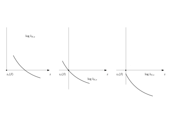
Figure 1: Graph of $\log\lambda_{\beta,z}$

(see for instance, [15, Theorem 4]).

The following is our main result of the article:

Theorem 2.

Let ${\mathcal{X}}$ be a mixing subshift of finite type in $\Sigma$. Let $\varphi$ be the potential function defined in (4). Then there exists a $\beta_{c}>0$ such that the following hold.

1. For $0<\beta<\beta_{c}$, there exists a unique equilibrium measure $\mu_{{}_{\beta}}$ characterized by complete support, and the pressure function is real analytic with $P(\beta)>\xi$.

2. For all $\beta>\beta_{c}$, $\mu_{{}_{{\mathcal{X}}}}$ stands as the singular equilibrium measure for the potential $\beta\varphi$, and it exhibits characteristics of not being fully supported while being significantly concentrated on the subshift ${\mathcal{X}}$. Moreover, the pressure function takes on an affine nature with $P(\beta)=\xi$, where $\xi$ signifies the entropy of X.

Furthermore, if $\beta_{c}=2$, the pressure function is a $C^{1}$-function.

4 Proof of Main theorem

4.1 Phase transition and Subshift of finite type

Let ${\mathcal{X}}$ be a mixing subshift of finite type. As every subshift of finite type is $k$-step shift of finite type and every $k$-step shift of finite type is a $1-step$ shift of finite type (see proposition 2.4), therefore, without any loss of generality, we assume that ${\mathcal{X}}$ is a 1-step shift of finite type. We denote $T_{{}_{\mathcal{X}}}$ be the associated transition matrix to subshift ${\mathcal{X}}$. Since ${\mathcal{X}}$ is mixing, therefore, there exists a $N_{{}_{\mathcal{X}}}\in{\mathbb{N}}$ such that $T_{{}_{\mathcal{X}}}^{n}>0$ for all $n\geq N_{{}_{\mathcal{X}}}$. We choose $N>>N_{{}_{\mathcal{X}}}$ large and by section 3.1, the potential function is defined as

$$\varphi(x)=\begin{cases}-\log\left(1+{1\over{\delta(x)}}\right)&\delta(x)\geq N\\ -A&\delta(x)<N.\end{cases}$$ (6)

Given that ${\mathcal{X}}$ is a 1-step shift of finite type. We can deduce the following; for any $i,j\in{\mathcal{S}}$, $ij\not\in L({\mathcal{X}})$, and let $J=[ij]$. Under this context $\varphi(x)=-A$, for all $x\in J$. Additionally, we denote ${\mathcal{F}}_{{}_{\mathcal{X}}}=\{x\in\Sigma_{{}_{\mathcal{S}}}:\delta(x)\leq N-1\}$, is the free region and ${\mathcal{E}}_{{}_{\mathcal{X}}}=\{x\in\Sigma_{{}_{\mathcal{S}}}:\delta(x)\geq N\}$ is the excursion region. It is evident that the cylinder $J\subset{\mathcal{F}}_{{}_{\mathcal{X}}}$ and ${\mathcal{X}}\subset{\mathcal{E}}_{{}_{\mathcal{X}}}$.

The set of return words

$${\mathcal{R}}_{J}=\{ijw:w\in L({\mathcal{X}})\,\,and\,\,jwi\in L({\mathcal{X}})\}.$$

Note that ${\mathcal{X}}$ is a mixing subshift, therefore, for each $n\geq N_{{\mathcal{X}}}$, there exists a $w\in L_{n}({\mathcal{X}})$ such that $iwj\in L({\mathcal{X}})$. This observation guarantees the existence of return word with length $n\geq N_{{\mathcal{X}}}$.

The spectral radius $\lambda_{\beta,z}$ is

$$\lambda_{\beta,z}=\sum\limits_{n\geq 1}\sum\limits_{|u|=n}e^{\beta S_{|u|}\varphi(ux)-|u|z},$$

for all $x\in J$. Concerning $N$, divide the above sum into two parts

$$\lambda_{\beta,z}=\sum\limits_{n=1}^{N-1}\sum\limits_{|u|=n}e^{\beta S_{|u|}\varphi(ux)-|u|z}+\sum\limits_{n\geq N}\sum\limits_{|u|=n}e^{\beta S_{|u|}\varphi(ux)-|u|z},$$

and let the identities

$${\mathcal{F}}(\beta,z)=\sum\limits_{n=1}^{N-1}\sum\limits_{|u|=n}e^{\beta S_{|u|}\varphi(ux)-|u|z}\,\,\,,and\,\,\,{\mathcal{E}}(\beta,z)=\sum\limits_{n\geq N}\sum\limits_{|u|=n}e^{\beta S_{|u|}\varphi(ux)-|u|z}.$$

Therefore,

$$\lambda_{\beta,z}={\mathcal{F}}(\beta,z)+{\mathcal{E}}(\beta,z).$$ (7)

We emphasize that, for any return word $u$ associated with cylinder set $J$, the following inequality always holds:

$$\delta(\sigma^{n}(ux))<\delta(\sigma^{n-1}(ux))-1,\,\,\,\,\,\,\,\,\,\,\,\,\,\,\,\,\,\,\,\,for\,\,all\,\,\,n\in[[2,|u|]].$$

i.e., there is no accident time except $1$ (for detail of accident we refer [12, 5]).

Let $u\in{\mathcal{R}}_{J}$, such that, $|u|\leq N-1$, then $S_{|u|}\varphi(ux)-|u|z)=-(A+z)|u|$, therefore,

$${\mathcal{F}}(\beta,z)=\sum\limits_{n=1}^{N-1}c_{n}e^{-\beta(A+z)n},$$

where $c_{n}$ is the multiplicity of return words with length $n$.  Let $u\in{\mathcal{R}}_{J}$, then for all $x\in J$,

$$S_{|u|}\varphi(ux)=\sum\limits_{i=0}^{|u|-1}\varphi\circ\sigma^{i}(ux)=-NA-\log\left(1+\frac{1}{n-1}\right)-\log\left(1+\frac{1}{n-2}\right)-\cdots\log\left(1+\frac{1}{N}\right),$$

$$S_{|u|}\varphi(ux)=-NA+\log N-\log n.$$

Consequently,

$${\mathcal{E}}(\beta,z)=e^{-\beta(NA-\log N)}\sum_{n\geq N}d_{n}\left(\frac{1}{n^{\beta}}\right)e^{-nz},$$

where $d_{n}$ is the multiplicity of return word of length $n\geq N$. Given that $N>>N_{{}_{{\mathcal{X}}}}$, since for each $i,j\in{\mathcal{S}}$, the number of path of length $n$, starting from digit $j$ and end the vertex $i$ is given by $T_{ji}^{n}$, that is the $(j,i)th$ entry of the matrix $T^{n}$. Using theorem 1, we get $C\alpha^{n}\approx d_{n}$, where $\alpha$ is the spectral radius of transition matrix $T$, and $C$ is the constant depends on $(j,i)th$ entry. We have

$${\mathcal{E}}(\beta,z)=Ce^{-\beta(NA-\log N)}\sum_{n\geq N}\Bigl{(}\frac{\alpha}{e^{z}}\Bigr{)}^{n}\frac{1}{n^{\beta}}.$$

The above series converges if and only if $\frac{\alpha}{e^{z}}<1$, equivalent to, $z\geq\xi$, where $\log\alpha=\xi$ is the entropy of the subshift ${\mathcal{X}}$.

By (7), we conclude that $\lambda_{\beta,z}$ converges for all $\beta\geq 0$ and $z_{c}(\beta)=\xi$. This implies that $z_{c}(\beta)=\xi$, for all $\beta\geq 0$. In order to find critical $\beta_{c}$

$$\lambda_{\beta,\xi}={\mathcal{F}}(\beta,\xi)+{\mathcal{E}}(\beta,\xi),$$

where,

$${\mathcal{F}}(\beta,\xi)=\sum\limits_{n=1}^{N-1}c_{n}e^{-\beta An},\,\,\,\,and,\,\,\,\,\,\,{\mathcal{E}}(\beta,\xi)=e^{-\beta C(A,N)}\sum\limits_{n\geq N}\frac{1}{n^{\beta}}.$$

Note that, $c_{n}\geq 0$, and $C(A,N)=NA-\log N>0$.

As $\frac{d}{d\beta}(\lambda_{\beta,\xi})\leq 0$, for all $\beta\geq 0$, therefore, $\lambda_{\beta,\xi}$ is a decreasing function. Furthermore, for $\beta\rightarrow 1$ then ${\mathcal{E}}(\beta,\xi)\rightarrow+\infty$, this implies $\lambda_{\beta,\xi}\rightarrow+\infty$, and if $\beta\rightarrow+\infty$, then, ${\mathcal{F}}(\beta,\xi)\rightarrow 0$, and ${\mathcal{E}}(\beta,\xi)\rightarrow 0$, therefore, $\lambda_{\beta,\xi}\rightarrow 0$. From the continuity and monotonicity of $\lambda_{\beta,\xi}$, there exists a $\beta_{c}>1$ such that $\lambda_{\beta_{c},\xi}=1$.

As a result, from [15, theorem 4]) and Figure 1, it follow that. For every $\beta<\beta_{c}$, it holds that $\lambda_{\beta,z}>1$ for all $z\geq\xi$. Since the function $z\rightarrow\lambda_{\beta,z}$ is characterized by monotonically decreasing behaviour, therefore, it can be inferred that there exists $z(\beta)>\xi$ such that $P(\beta)=z(\beta)$. Moreover, the there is a solitary equilibrium measure denoted by $\mu_{be}$, and the pressure function is endowed real analytic for each $\beta<\beta_{c}$.

Also, for each $\beta>\beta_{c}$, the function $\lambda_{\beta,z}<1$ for all $z\geq\xi$. Therefore, no equilibrium measure gives positive weight of cylinder $J$, and from 5, we conclude $P(\beta)=\xi$ for all $\beta>\beta_{c}$.

Consequently, the pressure function of potential $\varphi$ is as follows:

$$P(\beta)=\begin{cases}decreasing,convex\,\,and\,\,analytic&\forall\,\,\,\,\,\beta<\beta_{c}\\ \xi&\forall\,\,\,\,\,\,\beta>\beta_{c}\end{cases}$$ (8)

4.1.1 Regularity of Pressure function at $\beta_{c}$

The parameter $\beta_{c}$ signifies the threshold at which the pressure function undergoes a transition, as seen in (8). To assess the regularity of the pressure function at $\beta=\beta_{c}$, it’s essential to determine the count of equilibrium states at the transition point $\beta_{c}$. To achieve this, we will apply the theorem from [15, theorem 4]) in conjunction with the information presented in Figure 1(specifically, considering case III).

Proposition 4.1.

Let $\beta_{c}>1$ be the transition point for the pressure function, as detailed in (8). If $\beta_{c}=2$, the pressure function is a $C^{1}$-function. However, if $\beta_{c}$ deviates from 2, there is a possibility of encountering a first-order phase transition at $\beta_{c}$, contingent upon the characteristics of the equilibrium measure at $\beta_{c}$.

Proof.

As $\lambda_{\beta_{c},\xi}=1$, therefore, $P(\beta_{c})=\xi$ (see [15]). By 7 we get

$${\partial\over\partial z}\left(\lambda_{\beta,z}\right)={\mathcal{F}}^{\prime}(\beta_{c},\xi)+{\mathcal{E}}^{\prime}(\beta_{c},\xi).$$ (9)

at transition $\beta=\beta_{c}$ and $z=\xi$.

After a simple computation, we will able to get the following:

$${\mathcal{F}}^{\prime}(\beta_{c},\xi)=-\sum_{n=1}^{N-1}\frac{nc_{n}}{\alpha^{n}}e^{-\beta_{c}A},$$ (10)

and

$${\mathcal{E}}^{\prime}(\beta_{c},\xi)=-Ce^{-\beta_{c}(NA-\log N)}\sum_{n\geq N}\frac{1}{n^{\beta_{c}-1}}.$$ (11)

Since the series $\Sigma_{n\geq N}\frac{1}{n^{\beta_{c}-1}}$ exhibits a uniform asymptotic behaviour with Riemann zeta function $\zeta(\beta_{c}-1)$, which possess a pole at $\beta_{c}=2$. Therefore,

$${\partial\over\partial z}\left(\lambda_{\beta,z}\right)=+\infty,$$

at transition $\beta_{c}=2$ and $z=\xi$. By [15, theorem 4]) and Figure 1(case III), $\mu_{{}_{\mathcal{X}}}$ is the only equilibrium measure at $\beta_{c}$ and $P(\beta_{c})=\xi$.

For $\beta_{c}\not=2$, by the analytic continuation of Riemann $\zeta$-function $\zeta(\beta_{c}-1)<+\infty,$. Therefore, 9 exist if $\beta_{c}\not=2$. By [15, theorem 4]) and Figure 1(case III), there exists an equilibrium measure $\mu_{c}$ which has full support and $\mu_{c}(J)>0$. As $\varphi(x)=-A$ for all $x\in J$, therefore, $\int\phi d{\mu_{c}}\neq 0$. Given that, $P(\beta_{c})=\xi$, it follows that $\mu_{{}_{\mathcal{X}}}$ is the equilibrium measure at $\beta_{c}\varphi$. However, in this context, a scenario can arise where

$$\int\phi d{\mu_{c}}\neq\int\phi d\mu_{{}_{{\mathcal{X}}}},$$

holds, contingent upon the distinctive characteristics and formulations of measures $\mu_{c}$ and $\mu_{{}_{\mathcal{X}}}$. Consequently, the differentiability of the pressure function at $\beta_{c}\not=2$ may be subject to variation, determined by the specific attributes and properties of the measures involved.

∎

4.1.2 Examples

1. Hofbauer potential:

   Let ${\mathcal{X}}=\left\{0^{\infty}\right\}$, then $L\left(0^{\infty}\right)=\{0^{n}$ $:n\in{\mathbb{N}}\}$. Let $J=\left[1\right]$ and $A>0$, define the following potential,

   $$\varphi(x)=\begin{cases}-\log\left(1+{1\over{n}}\right)&x\in\left[0^{n}1\right]\\ -A&x\in\left[1\right]\end{cases}$$ (12)

   The function $\varphi$ is called the Hofbauer potential .
   

   The set ${\mathcal{R}}_{J}=\left\{10^{n}:n\in{\mathbb{N}}\cup\{0\}\right\}$ is the set of return word to cylinder $J$. For each $n\in{\mathbb{N}}$, there is only one $u\in{\mathcal{R}}_{J}$ such that $|u|=n$. By a detailed computation from [15, section 3.3], the spectral radius $\lambda_{\beta,z}$ is as follows:

   $$\lambda_{\beta,z}=e^{-\beta A}\sum\limits_{n=0}^{\infty}\left(\frac{1}{n+1}\right)^{\beta}e^{-z(n+1)}.$$

   Furthermore, $\beta\geq 0$, we have $z_{c}(\beta)=0$, and there exists a critical $\beta_{c}$ such that $\lambda_{\beta_{c},0}=1$. By [15, theorem 4]),the pressure function of the Hofbauer potential admits a phase transition at $\beta_{c}$.

   Indeed, the pressure function of Hofbauer has the following form:

   $$P(\beta)=\begin{cases}decreasing,convex\,\,and\,\,analytic&\forall\,\,\,\,\,\beta<\beta_{c}\\ 0&\forall\,\,\,\,\,\,\beta>\beta_{c}\end{cases}$$

   See figure 2.
   

   Furthermore, $\delta_{0^{\infty}}$ is the only equilibrium measure at the transition parameter $\beta_{c}$, when $\beta_{c}=2$. Since derivative of spectral radius at $\beta=\beta_{c}$ and $z=0$ is as follows:

   $${\partial\over\partial z}\left(\lambda_{\beta,z}\right)=e^{-\beta_{c}A}\zeta(\beta_{c}-1)$$ (13)

   Using the above argument in 4.1.1. $\zeta(\beta_{c}-1)$ has a simple pole at $\beta_{c}=2$, and $\zeta(\beta_{c}-1)=+\infty,$ at $\beta_{c}=2$, and 13 does not exist. Therefore, $\delta_{0^{\infty}}$ is the only equilibrium measure at $\beta_{c}$ and the pressure function is $C^{1}$-continuous.
   On the other side, for $\beta_{c}\not=2$, by the analytic continuation of Riemann $\zeta$-function $\zeta(\beta_{c}-1)<+\infty$. Therefore, 13 exist if $\beta_{c}\not=2$, this ensures the existence of a fully supported equilibrium measure $\mu_{c}$ such that $\int\phi d{\mu_{c}}\neq 0$. Since, $\delta_{0^{\infty}}$ is another equilibrium measure of $\beta_{c}\varphi$, and $\int\phi d\delta_{0^{\infty}}=0$, this implies the pressure function of Hofbauer potential is not differentiable at $\beta_{c}$.

2. Golden mean Subshift:
   

   Let ${\mathcal{X}}=\Sigma_{{}_{11}}$ be the Golden-mean subshift, then

   $$L(\Sigma_{{}_{11}})=\{w\in\Sigma^{+}:w_{i}w_{i+1}\not=11\,\,,\,\forall\,\,0\leq i\leq|w|-1\}.$$

   Let $J=[11]$, then $\delta(x)=1$, for all $x\in J$. Let $N>>1$, and $A>1$, define the following potential,

   $$\varphi(x)=\begin{cases}-\log\left(1+{1\over{\delta(x)}}\right)&\delta(x)\geq N\\ -A&\delta(x)<N.\end{cases}$$ (14)

   The set of return words

   $${\mathcal{R}}_{J}=\{11w:w\in L(\Sigma_{{}_{11}})\,\,and\,\,w_{0}\not=1\}.$$

   For each $n\in{\mathbb{N}}$, $card\left({L_{n}}\left(\Sigma_{{}_{11}}\right)\right)=F_{n}$, where $F_{n}$ is the $n$th Fibonacci word. Given that the transition matrix to Golden mean subshift is as follows:

   $$G=\left[{\begin{array}[]{cc}1&1\\ 1&0\\ \end{array}}\right]$$

   for each $n\in{\mathbb{N}}$, we have

   $$G^{n}=\left[{\begin{array}[]{cc}F_{n}&F_{n-1}\\ F_{n-1}&F_{n-2}\\ \end{array}}\right]$$

   $F_{n-2}$ is the number of factors that starts from digit 1 and end at digit 1 in $L_{n}\left(\Sigma_{{}_{11}}\right)$.

   The spectral radius $\lambda_{\beta,z}$ can be formulate as follows is

   $$\lambda_{\beta,z}=\sum\limits_{n\geq 1}F_{n-2}e^{\beta S_{|u|}\varphi(ux)-|u|z},$$

   for all $x\in J$. Since for large $n\geq N$, we have $F_{n}\approx\gamma^{n}$ (Binet formula), where $\gamma$ is the golden ratio and the spectral radius of matrix $G$.

   A computation from section 4.1, we will able to get the pressure function of $\varphi$ in (14) has the following form

   $$P(\beta)=\begin{cases}decreasing,convex\,\,and\,\,analytic&\forall\,\,\,\,\,\beta<\beta_{c}\\ \log\gamma&\forall\,\,\,\,\,\,\beta>\beta_{c}\end{cases}$$

   

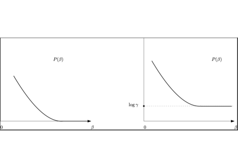
   Figure 2: Graph of $P(\beta)$ in Hofbauer’s and Golden-mean cases

References

- [1] Alexandre Tavares Baraviera, Renaud Leplaideur, and Artur Oscar Lopes. Ergodic optimization, zero temperature limits and the max-plus algebra. arXiv preprint arXiv:1305.2396, 2013.
- [2] R Bowen. Equilibrium states and the ergodic theory of anosov diffeomorphisms second revised edition. LECTURE NOTES IN MATHEMATICS-SPRINGER-VERLAG-, 470(2), 2008.
- [3] Rufus Bowen. Ergodic theory of axiom a diffeomorphisms. In Equilibrium States and the Ergodic Theory of Anosov Diffeomorphisms, pages 90–107. Springer, 1975.
- [4] Henk Bruin and Renaud Leplaideur. Renormalization, thermodynamic formalism and quasi-crystals in subshifts. Communications in Mathematical Physics, 321(1):209–247, Feb 2013.
- [5] Henk Bruin and Renaud Leplaideur. Renormalization, freezing phase transitions and fibonacci quasicrystals. Annales scientifiques de l’École normale supérieure, 48(3):739–763, 2015.
- [6] Henk Bruin and Mike Todd. Wild attractors and thermodynamic formalism. Monatshefte für Mathematik, 178(1):39–83, 2015.
- [7] Franz Hofbauer. Examples for the nonuniqueness of the equilibrium state. Transactions of the American Mathematical Society, 228:223–241, 1977.
- [8] Franz Hofbauer and Gerhard Keller. Equilibrium states for piecewise monotonic transformations. Ergodic Theory and Dynamical Systems, 2(1):23–43, 1982.
- [9] Roger A Horn and Charles R Johnson. Matrix analysis. Cambridge university press, 2012.
- [10] Godofredo Iommi and Mike Todd. Thermodynamic formalism for interval maps: inducing schemes. Dynamical Systems, 28(3):354–380, Sep 2013.
- [11] Godofredo Iommi and Mike Todd. Transience in dynamical systems. Ergodic Theory and Dynamical Systems, 33(5):1450–1476, 2013.
- [12] Shamsa Ishaq and Renaud Leplaideur. An estimation of phase transition. Nonlinearity, 35(3):1311, 2022.
- [13] Renaud Leplaideur. Local product structure for equilibrium states. Transactions of the American Mathematical Society, 352(4):1889–1912, 2000.
- [14] Renaud Leplaideur. Chaos : Butterflies also generate phase transitions and parallel universes, 2013.
- [15] Renaud Leplaideur. From local to global equilibrium states: Thermodynamic formalism via an inducing scheme. Electronic Research Announcements, 21(0):72–79, 2014.
- [16] Douglas Lind and Brian Marcus. An introduction to symbolic dynamics and coding. Cambridge university press, 1995.
- [17] Monsieur Lothaire. Algebraic combinatorics on words, volume 90. Cambridge University Press, 2002.
- [18] David Ruelle. Thermodynamic formalism: the mathematical structure of equilibrium statistical mechanics. Cambridge University Press, 2004.
- [19] Omri M Sarig. Thermodynamic formalism for countable markov shifts. Ergodic Theory and Dynamical Systems, 19(6):1565–1593, 1999.
- [20] Omri M Sarig. Phase transitions for countable markov shifts. Communications in Mathematical Physics, 217(3):555–577, 2001.
- [21] Omri M Sarig. Thermodynamic formalism for null recurrent potentials. Israel Journal of Mathematics, 121(1):285–311, 2001.
- [22] Yakov G Sinai. Gibbs measures in ergodic theory. Russian Mathematical Surveys, 27(4):21, 1972.
- [23] Peter Walters. A variational principle for the pressure of continuous transformations. American Journal of Mathematics, 97(4):937–971, 1975.
- [24] Peter Walters. An introduction to ergodic theory, volume 79. Springer Science & Business Media, 2000.