Sherlock Holmes Doesn’t Play Dice:
The significance of Evidence Theory for the Social and Life Sciences

Abstract

While Evidence Theory (Demster-Shafer Theory, Belief Functions Theory) is being increasingly used in data fusion, its potentialities in the Social and Life Sciences are often obscured by lack of awareness of its distinctive features. With this paper we stress that Evidence Theory can express the uncertainty deriving from the fear that events may materialize, that one has not been able to figure out. By contrast, Probability Theory must limit itself to the possibilities that a decision-maker is currently envisaging.

Subsequently, we illustrate how Dempster-Shafer’s combination rule relates to Bayes’ Theorem for various versions of Probability Theory and discuss which applications of Information Theory can be enhanced by Evidence Theory. Finally, we illustrate our claims with an example where Evidence Theory is used to make sense of the partially overlapping, partially contradictory solutions that appear in an auditing exercise.

Keywords: Evidence Theory, Belief Functions, Dempster-Shafer, Radical Uncertainty, Unknown Unknowns, Human-Computer Interaction, Large Language Models

1 Introduction

Sometimes, unexpected and novel events upset the network of causal relations on which we base our decisions. A global pandemic in the XXI century, a local conflict that might degenerate into World War III, as well the 2008 financial crisis are global and well-known examples of events that had not been conceived before they actually happened, with the consequence of generating a simple but fundamental question: “Now, what else?” Similarly to political instability, also technological innovations question existing business models, increasing resistance to antibiotics question the reliability of available cures, not to speak of the vagaries of company politics that question career paths nearly every day. The key feature of all these events is that decision-makers had not been able to figure them out in advance, and therefore, they induce decision-makers to think that other novel and potentially disruptive possibilities may materialize. This state of mind cannot be dealt by Probability Theory, because it starts with the assumption that the set of possibilities is a given. Nevertheless, it has been hotly debated in economics because it has a huge impact on private investments and, with a ripple effect, consumption and unemployment.

This sort of non-probabilistc uncertainty, which has been eventually qualified as “Keynesian,” “fundamental,” “true,” “epistemic,” “ontological” and more recently “radical” uncertainty [35] [7] [15] [9] [29] [24] should be clearly distinguished from the uncertainty deriving from lack of reliability originating, among else, from the paucity of the sample on which probabilities are measured. Small sample size, unfair dice and unique events pose serious problems to the assessment of reliable probabilities, but they still concern given events. With a possibly awkward but dense expression the literature traces a clear distinction between “known unknowns” (unknown probabilities of known possibilities) and “unknown unknowns” (unknown probabilities of unknown possibilities) [34] [17] [16].

Subjective interpretations can stretch Probability Theory up to encompass known unknowns, eventually resorting to imprecise and sub-additive probabilities. However, the conceptual framework of Probability Theory impairs it from dealing with unknown unknowns, i.e., the radical uncertainty originating from the feeling that the possibilities that are being envisaged may not be exhaustive.

The reason for writing this essay is that Glenn Shafer’s Evidence Theory [42] overcomes this limitation by not assuming that the complementation operation is defined on the possibility set. Without complementation, no residual event can be defined. Radical uncertainty on “what else may happen” can not be channeled into a residual event but rather remains unassigned, hovering above the frame of discernment and influencing the computations on the possibilities that are being envisaged without ever being pinned down to any of them. Conflicting evidence make it increase, consonant evidence make it decrease, but the framework is such that there is always room for the suspicion that the unthinkable may occur.

Possibly because most data fusion applications work with a given set of sources and possibilities, this aspect of Evidence Theory has been somehow neglected hitherto. Most of the mathematical literature focuses on isolated components of the theory, namely Belief Functions and Dempster-Shafer’s combination rule, to the point that Evidence Theory has come to be known as “Demsper-Shafer Theory” or “Belief Functions Theory” rather than with its original name. We rather prefer to revert to the early usage also because — as we shall remind in § 3.1 — Dempster-Shafer’s combination rule and Belief Functions are also employed in extensions of Probability Theory that can deal at most with known unknowns. By contrast, we focus on the radical uncertainty generated by unknown unknowns, which requires a radically different conceptual framework.

In particular, we are concerned with the fact that many mathematical refinements of Evidence Theory neglect that its canonical setting is a judge listening to testimonies or a detective looking for clues, rather than a gambler playing dice. This is critical, because while it is natural for a gambler to reason in terms of a given set of outcomes, a detective must be open to unexpected denouements.

The rest of this paper is organized as follows. The ensuing section § 2 illustrates the basics of Evidence Theory highlighting its ability to encompass both known and unknown unknowns. Contrary to most summaries, it emphasizes the human role in formulating hypotheses upon which beliefs may be hold, that are supported by the available evidence. Subsequently, § 3 frames Evidence Theory with respect to Probability Theory and Information Theory, respectively. In particular, § 3.1 illustrates the ability of Probability Theory to deal with known unknowns by employing tools from Evidence Theory whereas § 3.2 discusses the usefulness of employing Evidence Theory in the problem of information transmission through a genome. Section § 4 illustrates the above points with a numerical example from auditing. Finally, section § 5 concludes with remarks on the importance of adding theory to the current wave of applications.

2 Radical Uncertainty Within Evidence Theory

This brief introduction to Evidence Theory aims at highlighting its ability to express radical uncertainty. It is neither complete nor mathematically sophisticated, but rather highlights this theory’s capability to handle exotic forms of uncertainty.

In Evidence Theory, the possibility set is called frame of discernment in order to stress that it represents what possibilities a decision-maker is envisaging at a certain point in time. A frame of discernment $\Theta$ may entail possibilities $A_{1},$ $A_{2},\ldots$ $A_{N}$ that are supported by masses of empirical evidence $m(A_{1}),$ $m(A_{2}),\ldots$ $m(A_{N})$. However, those $m_{i}(.)$ are not probabilities because $\Theta$ is not a $\sigma$-algebra. In particular, $\Theta$ lacks the complementation operation. Notably, this makes it possible for a decision-maker to contemplate a mass $m(\Theta)>0$ which is not committed to any possibility but rather expresses a sense that “unknown unknowns” might exist. Let us assume that this state of affairs has been originated by empirical evidence in the form $\{m(A_{1}),$ $m(A_{2}),\ldots$ $m(\Theta)\}$ where the incoming $m(\Theta)$ supports the conviction that something else may happen.

Though not essential to the theory, masses $m(.)$ can be normalized in order to obtain that:

$$\sum_{i=1}^{N}\>m_{i}(A_{i})\;+\;m(\Theta)\;=\;1$$ (1)

However, since possibilities $A_{i}$ are not necessarily disjoint sets, eq. 1 does not amount to distributing a given mass among given possibilities. In particular, if $\exists i,j:A_{i}\cap A_{j}\neq\emptyset$, then $m(A_{i})+m(A_{j})$ is not equivalent to $m(A_{i}\cup A_{j})$ as it is the case with probabilities.

It is important to realize that eq. 1 expresses a feature of incoming evidence rather than the representation of a decision process implied by a $\sigma$-algebra. Perhaps inadvertently, by assuming that all logical operations are necessarily carried out Probability Theory has made a similar assumption to that of classical AI, namely that all reasoning is based on symbolic logic. This interpretation has been challenged by neural-network-based association of stimuli and emergence of concepts [6], but probabilistic treatment of uncertainty has apparently ignored the connectionist revolution hitherto. We concede that logical operations make perfect sense in the restricted environment of games of chance, but not necessarily elsewhere.

Evidence Theory does not take a gambler as its prototypical subject, but rather a judge or a detective [40] [43]. Contrary to gamblers who know the faces of a die or the numbers on a roulette, judges and detectives are aware that unexpected clues and testimonies may open up novel possibilities. For many crucial decision-making contexts, ranging from managers making investments to politicians warping alliances or employees trying to make a career, the canonical situation of a detective looking for cues may be more relevant than that of gamblers looking for luck.

Let us consider a frame of discernment $\Theta$. Let us denote as $\{m(A_{1}),$ $m(A_{2}),\ldots$ $m(\Theta)\}$ the body of evidence that is currently available, where the $A_{i}$s are not necessarily disjoint sets.

Suppose that a new body of evidence arrives (a new testimony, new cues, etc.), which we may denote as $\{m(B_{1}),$ $m(B_{2}),\ldots$ $m(\Theta)\}$. Just like the sets entailed in one single body of evidence are not necessarily disjoint, $\forall i,j$ it may be $A_{i}\subseteq B_{j}$, $A_{i}\supseteq B_{j}$, $Ai\cap B_{j}\neq\emptyset$ or $A_{i}\cap B_{j}=\emptyset$.

The judge, or detective, must make sense of both bodies of evidence, evaluating which items are coherent with one another while weighing them against contradictory pieces of evidence. Dempster-Shafer’s combination rule [8] [42] yields the components of a new body of evidence that unites the previous ones:

$$m(C_{k})\;=\;\frac{\sum_{A_{i}\cap B_{j}=C_{k}}\;m(A_{i})\,m(B_{j})}{1-\>\sum_{A_{i}\cap B_{j}=\emptyset}\;m(A_{i})\,m(B_{j})}$$ (2)

where the $C_{k}$s are defined by all possible intersections of the $A_{i}$s and the $B_{j}$s. Since $A_{i}\cap\Theta=A_{i}$ and $B_{j}\cap\Theta=B_{j}$, eq. 2 can be evidently used to compute $m(\Theta)$, too.

The numerator of eq. 2 measures the extent to which the two bodies of evidence support $C_{k}$, whereas the denominator measures the extent to which they are not contradictory with one another. In the simplest, 1-dimensional case [41], information is conveyed through a series of $n$ testimonies of reliability $m$ each, yielding a combined reliability $m^{n}$. By contrast, the combined reliability of $n$ independent parallel testimonies is $1-(1-m)^{n}$. Thus, in eq. 2 the numerator expresses the logic of serial testimonies whereas the denominator expresses the logic of parallel testimonies.

Masses $m(.)$ can be discounted in order to account for the reliability of testimonies, or the existence of correlation between different bodies of evidence. By contrast, “known unknowns” are not handled by affecting masses $m(.)$ as it happens in Probability Theory.

Consider the case of insurance companies facing the problem of evaluating the cost of adverse events without reliable samples, which is where the problem of known unknowns was first identified in economics [27]. Wildfires favoured by climate change are a good point in case, because the probabilities that had been measured decades ago no longer apply today. Uncertainty concerns a known possibility (wildfires), but the problem is that its new probability is unknown, or only partially known. Probability Theory expresses this known unknown by means of probability intervals (wildfires may occur with, say, some unknown probability greater than $0.01$ but smaller than $0.1$), whereas Evidence Theory takes on quite a different route.

In Evidence Theory, possibilities are sets whose elements can differ in a number of details. Thus, Evidence Theory would rather attempt to discriminate climate-change-induced wildfires with respect to the previous ones, for instance in terms of the length of the dry season, firefighters’ equipment, the strength and direction of winds in a specific area, or else. In the frame of discernment, climate-changed-induced wildfires would partially overlap with the traditional ones. Evidence Theory would express this “known unknown” by means of the extent of this overlap, as well as the difference between the extremes of the probability interval that Probability Theory would use. More on this in § 3.1.

Dempster-Shafer’s combination rule can be iterated to combine any number of evidence bodies. Its outcome is independent of the sequence in which evidence bodies arrive. Along iterations, coherent masses of evidence reinforce one another whereas incoherent evidence has the effect of increasing $m(\Theta)$, or even generating it anew.

In the course of a process of evidence collection and combination, eq. 2 can be iterated any number of times on bodies of evidence that are eventually normalized by means of eq. 1. The ensuing combined evidence can be used to support specific hypotheses.

Let us now suppose that the decision-maker (a judge, a detective, etc.) formulates a hypothesis $\mathcal{H}$. The belief (s)he can reasonably entertain on $\mathcal{H}$ is given by the amount of evidence supporting it. Assuming a body of evidence $\{m(C_{1}),$ $m(C_{2}),\ldots$ $m(\Theta)\}$, the belief in $\mathcal{H}$ is expressed by Belief Function:

$$Bel(\mathcal{H})\;=\sum_{C_{k}\subset\mathcal{H}}m(C_{k})$$ (3)

where, by definition, $Bel(\emptyset)=0$ and $Bel(\Theta)=1$.

While belief in $\mathcal{H}$ is only supported by the evidence bearing specifically on $\mathcal{H}$, the Plausibility Function includes also the evidence that partially supports $\mathcal{H}$:

$$Pl(\mathcal{H})\;=\sum_{C_{k}\cap\mathcal{H}\neq\emptyset}m(C_{k})$$ (4)

where, by definition, $Pl(\emptyset)=0$ and $Pl(\Theta)=1$.

Obviously, $Bel(\mathcal{H})\leq Pl(\mathcal{H})$. In most applications, belief is more important than plausibility.

Note also that while the frame of discernment cannot generate residual events out of complementation, the judge or detective can. Thus, $Bel(\mathcal{H})+Bel(\overline{\mathcal{H}})\leq 1$, $Pl(\mathcal{H})+Pl(\overline{\mathcal{H}})\geq 1$, and $Pl(\mathcal{H})=1-Bel(\overline{\mathcal{H}})$. Once again, logic is possible for humans though it is not necessarily embodied in the (connectionist?) ways humans process incoming information.

In general, decision-makers may formulate several alternative hypotheses, which they may wish to compare to one another given the available evidence. For instance, hypotheses $\mathcal{H}_{1}$ and $\mathcal{H}_{2}$ can be compared by evaluating whether $Bel(\mathcal{H}_{1})\lessgtr Bel(\mathcal{H}_{2})$.

Let us denote $\mathbf{\mathcal{H}}^{t}=$ $\{\mathcal{H}_{1}^{t},$ $\mathcal{H}_{2}^{t},\ldots$ $\mathcal{H}_{n_{t}}^{t}\}$ the set of hypotheses that a decision-maker is entertaining at time $t$, and let us denote $\mathbf{\mathcal{H}}^{t+1}=$ $\{\mathcal{H}_{1}^{t+1},$ $\mathcal{H}_{2}^{t+1},\ldots$ $\mathcal{H}_{n_{t+1}}^{t+1}\}$ the set of hypotheses at time $t+1$. In general, $\mathcal{H}_{k}^{t+1}\neq\mathcal{H}_{k}^{t}$ $\forall k,t\in\mathcal{\mathbb{N}}$, and even $n_{t+1}\neq n_{t}$. Hypotheses can change with time, and even their number can.

The alternative hypotheses that are being entertained can either change out of some behavioral algorithm simulating human reasoning, or actual participation of a human being in subsequent interactions with an expert system, or they may be simply suggested by subsequent iterations of eq. 2, in which case $\mathcal{H}_{k}\equiv C_{k}$. Or, some combination of the above cases. Note that Evidence Theory does not impose any constraint on this.

Albeit only crisp sets have been assumed hitherto and will be considered henceforth, Evidence Theory has been extended to fuzzy sets [14] [26]. Notably, this extension is not possible for Probability Theory because it requires possibilities to be mutually exclusive.

3 Evidence, Probability, and Information Theories

In this section we relate Evidence Theory to Probability Theory and Information Theory, respectively. In particular, in § 3.1 we re-interpret Bayes’ Theorem as a special case of eq. 2 when evidence presents itself as probabilities; by contrast, a version of eq. 2 is still needed for imprecise probabilities. In § 3.2 we show that Evidence Theory is the appropriate framework when Shannon’s Information Theory is applied to information transmission through the genome.

We do not show the numerical details. For detailed comparisons between Bayes’ Theorem and Dempster-Shafer combination rule, please see [5] [12] [47].

3.1 Evidence Theory and Probability Theory

While there exist several accounts of the specific cases where Dempster-Shafer combination rule can be interpreted within Probability Theory [46], we rather explore how Bayes’ rule can be understood by Evidence Theory. Specifically, we illustrate the special cases in which, within Evidence Theory, eq. 2 boils down to Bayes’ rule.

The following assumptions are — among else — implied by Probability Theory:

1. All possibilities are singletons, in which case $\forall\{A_{i}\}$ and $\forall\{B_{j}\}$ it is either $\{A_{i}\}\cap\{B_{j}\}\equiv$ $\{A_{i}\}\equiv$ $\{B_{j}\}$ or $\{A_{i}\}\cap\{B_{j}\}=\emptyset$. In other words, possibilities are not sufficiently nuanced to enable partial overlap. One immediate consequence is that no $C_{k}$ appears anymore in eq. 2 because it is not possible to generate possibilities beyond those that are included in the incoming bodies of evidence.

2. Although novel possibilities can present themselves, no belief can be allocated to the fear that this may happen. Thus, $m(\Theta)=0$ and, therefore, the bodies of evidence to be combined take the form $p(\{A_{1}\}),$ $p(\{A_{2}\}),\ldots$ $p(\{A_{M}\})$ and $p(\{B_{1}\}),$ $p(\{B_{2}\}),\ldots$ $p(\{B_{N}\})$, respectively, where $M,N\in\mathbb{N}$. Probabilities $p$ are subject to the usual constraints $\sum_{i}p(\{A_{i}\})=1$ and $\sum_{j}p(\{B_{j}\})=1$.

Let us assume that beliefs are automatically generated by the combination of evidence, hence eqs. 3 and 4 are not necessary. Furthermore, because of condition (i) beliefs at different points in time can be expressed in terms of prior evidence $\{p(\{A_{1}\}),$ $p(\{A_{2}\}),\ldots$ $p(\{A_{N}\})\}$. Thus beliefs are updated, but these updates coincide with prior and posterior probabilities on the initial set:

Prior Probability:

$Bel^{t}(\mathcal{H}_{i})\equiv p(\{A_{i}\})$, $\forall i$

Posterior Probability:

$Bel^{t+1}(\mathcal{H}_{i})\equiv p(\{A_{i}\}\mid\{B_{j}\})$, $\forall i,j$

For simplicity, and without loss of generality, let us assume that $\exists p,q:\{A_{p}\}\equiv\{B_{q}\}$ whereas $\forall i,j\neq\{p,q\}$ it is $\{A_{i}\}\cap\{B_{j}\}=\emptyset$. Let us feed eq. 2 into $Bel^{t+1}(\mathcal{H}_{p})$ while highlighting the time stamp by means of a superscript:

$$\begin{array}[]{ccccc}p(\{A_{p}^{t}\}\mid\{B_{q}^{t+1}\})&\stackrel{{\scriptstyle(a)}}{{=}}&\frac{p(\{A_{p}^{t}\})\;p(\{B_{q}^{t+1}\})}{1\;-\;\sum_{\begin{subarray}{c}i\neq p\\ j\neq q\end{subarray}}\;p(\{A_{i}^{t}\})\;p(\{B_{j}^{t+1}\})}&\stackrel{{\scriptstyle(b)}}{{=}}&\frac{p(\{B_{q}^{t}\})\;p(\{A_{p}^{t+1}\})}{p(\{B_{q}^{t+1}\})}\\ &&&&\\ &\stackrel{{\scriptstyle(c)}}{{=}}&\frac{p(\{B_{q}^{t}\}\mid\{A_{p}^{t+1}\})\;p(\{A_{p}^{t+1}\})}{p(\{B_{q}^{t+1}\})}&&\end{array}$$

which is Bayes’ Theorem for $\{A_{p}\}$ and $\{B_{q}\}$.

Passage (a) is a straightforward application of eq. 2. The denominator of passage (b) is obtained by remarking that albeit $\{A_{p}^{t}\}$ and $\{B_{q}^{t+1}\}$ overlap, $\{B_{q}^{t+1}\}$ comes at a later point in time. The numerator of passage (b), as well as passage (c), require a time inversion of the arrival of bodies of evidence $\{p(\{A_{1}\}),p(\{A_{2}\}),\ldots p(\{A_{N}\})\}$ and $\{p(\{B_{1}\}),p(\{B_{2}\}),\ldots p(\{B_{N}\})\}$, respectively. This is possible because the sequence of arrival has no impact on Dempster-Shafer rule and, in any case, this is the very same logic employed in the standard demonstration of Bayes’ theorem.

However, Probability Theory has been greatly extended beyond conditions (i) and (ii). In particular, imprecise probabilities can be defined over an interval $[p_{*},p^{*}]$ where $p_{*}$ is called a lower probability and $p^{*}$ is an upper probability. Empirical measurement is expected to elicit that $p\in$ $[p_{*},p^{*}]$ rather than assessing some exact value for $p$.

Imprecise probabilities are not additive, for $\sum_{i}p_{*}(\{A_{i}\})\leq 1$ and $\sum_{i}p^{*}(\{A_{i}\})\geq 1$. However, $p^{*}(\{A_{i}\})=1-p_{*}(\{\overline{A}_{i}\}),\forall i$. Conditions (i) and (ii) become:

1. All possibilities are singletons, in which case $\forall\{A_{i}\}$ and $\forall\{B_{j}\}$ it is either $\{A_{i}\}\cap\{B_{j}\}\equiv$ $\{A_{i}\}\equiv$ $\{B_{j}\}$ or $\{A_{i}\}\cap\{B_{j}\}=\emptyset$. Thus, possibilities are not sufficiently nuanced to enable partial overlap. One immediate consequence is that no $C_{k}$ appears anymore in eq. 2 because it is not possible to generate possibilities beyond those suggested by the incoming bodies of evidence.

2. Although novel possibilities can present themselves, no belief can be allocated to the fear that this may happen. Thus, $m(\Theta)=0$ and, therefore, the bodies of evidence to be combined can be expressed as $\{[p_{*}(\{A_{1}\}),$ $p^{*}(\{A_{1}\})],$ $[p_{*}(\{A_{2}\}),$ $p^{*}(\{A_{2}\})]\ldots$ $[p_{*}(\{A_{M}\}),$ $p^{*}(\{A_{N}\})]\}$ and $\{[p_{*}(\{B_{1}\}),$ $p^{*}(\{B_{1}\})],$ $[p_{*}(\{B_{2}\}),$ $p^{*}(\{B_{2}\})],\ldots$ $[p_{*}(\{B_{N}\}),$ $p^{*}(\{B_{N}\})]\}$, respectively, with $M,N\in\mathbb{N}$.

where (i)’ is obviously equivalent to (i).

Imprecise probabilities can usefully express partial knowledge of a stochastic process, for instance when it is unclear which specific probability distribution is generating it. Furthermore, in empirical investigations experts often naturally express themselves in terms of probability intervals rather than precise values.

Finally, imprecise probabilities can be used to combine probabilistic uncertainty with the uncertainty deriving from relying on too small a sample. Suppose, for instance, that you are playing for the first time with a die that you suspect may not be fair. Lack of information may prudentially suggest $p\in[1/7,\,1/5]$ rather than $p=1/6$. Later on, by throwing the die again and again the intervals shrink down to the true, precise probabilities.

When imprecise probabilities are employed to include the uncertainty due to sample size, upper probabilities are sometimes neglected. The remaining lower probabilities are eventually called sub-additive probabilities, to which the standard probability calculus applies [21] [36]. In particular, a body of evidence $\{p_{*}(\{A_{1}\}),$ $p_{*}(\{A_{2}\}),\ldots$ $p_{*}(\{A_{M}\})\}$ can be conditioned on $\{p_{*}(\{B_{1}\}),$ $p_{*}(\{B_{2}\}),\ldots$ $p_{*}(\{B_{N}\})\}$ by means of Bayes’ rule [23].

In the general case, imprecise probabilities on singletons can be handled just like precise probabilities on partially overlapping sets [48] [18]. In order to grasp the rationale for this transformation, suppose that you are dealing with an unfair die where face 1 shows up more often than $1/6$ because some lead has been injected just below face 6. Thus, faces 2, 3, 4 and 5 show up less often and face 6 least often. You can understand it as if a small portion of the events “face 2” to “face 5,” and a large portion of the event “face 6” are turned into the event “face 1.” You should have observed, e.g., face 2, but you observe face 1 in fact.

Figure 1 illustrates this transformation for 1-dimensional sets, i.e., intervals. Note that with this transformation we obtain the framework of Evidence Theory, which is based on sets $A_{i}$ rather than singletons $\{A_{i}\}$.

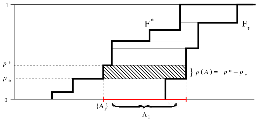
Figure 1: Transformation of imprecise probabilities defined on singletons into single-valued probabilities defined on intervals. Step-wise cumulative lower probability function $F_{*}$ and upper probability function $F^{*}$ identify intervals $A_{i}$ with probability $p(A_{i})=p^{*}-p_{*}$. Notably, for any $(i,i\,^{\prime})$ it may happen that $A_{i}\cap A_{i\>^{\prime}}\neq\emptyset$.

This transformation is not one-to-one because of special cases when singletons appear along with intervals in the Dempster-Shafer structure [48] [18]. However, the duality of singleton-based imprecise probabilities and set-based single-valued probabilities allows us to re-formulate assumptions (i)’ and (ii)’ as follows:

1. Possibilities are represented by sets $A_{1},$ $A_{2}\ldots$ $A_{M}$ that may intersect one another. Thus, new possibilities $C_{k}$can be generated by eq. 2.

2. Although novel possibilities can present themselves, no belief can be allocated to the fear that this may happen. Thus, $m(\Theta)=0$ and, therefore, the bodies of evidence to be combined take the form $p(A_{1}),$ $p(A_{2}),\ldots$ $p(A_{M})$ and $p(B_{1}),$ $p(B_{2}),\ldots$ $p(B_{N})$, respectively, where $M,N\in\mathbb{N}$. Probabilities $p$ are subject to the constraints $\sum_{i}p(A_{i})=1$ and $\sum_{j}p(B_{j})=1$ but, since the $A_{i}$s and $B_{j}$ may overlap, these conditions do not have the same meaning as in standard Probability Theory.

With conditions (i)” and (ii)” we are still within Probability Theory, but bodies of evidence must be combined by means of Dempster-Shafer rule 2. The differences with Evidence Theory are that (a) probabilities $p$ appear instead of masses $m$, and (b) $m(\Theta)$ is ignored.

One remarkable conclusion is that Dempster-Shafer’s combination rule, as well as belief and plausibility functions induced by partially overlapping probability sets, are well within (an extended version of) Probability Theory. Indeed, Arthur Dempster moved initially from imprecise probabilities to propose eq.2 [8].

However, it is important to stress that Probability Theory applies to situations that can be likened to a gambler playing a game of chance, whereas Evidence Theory applies to situations that remind of a detective looking for cues. One important difference is that in the first case the possibility set is known, whereas in the second case possibilities are framed while they are being received. In the first case, only known unknowns are possible, whereas in the second case unknown unknowns can be considered as well.

In this sense, substituting the expression “Evidence Theory” with “Dempster-Shafer Theory” or “Theory of Belief Functions” can be misleading, because the last two expressions concern Probability Theory as well. Both Probability Theory and Evidence Theory have something to say on uncertain reasoning but, since they are based on different paradigms, they should not be confused with one another.

3.2 Evidence Theory and Information Theory

A detective looking for clues or a judge evaluating testimonies receive bodies of evidence, which they must compare to one another in order to form beliefs and formulate hypotheses. This situation is quite opposite to that of a gambler playing a game of chance, but it is not far from receiving information through a noisy channel. Indeed, Shafer and Tversky [43] have cast Evidence Theory in terms of information transmission.

Shannon’s Information Theory assumes that the receiver of characters drawn out of a set $B=\{\{B_{1}\},\{B_{2}\},\ldots\{B_{N}\}\}$ through a noisy channel must infer which characters, out of a set $A=\{\{A_{1}\},\{A_{2}\},\ldots\{A_{N}\}\}$, a source actually emitted. Since the receiver knows the set of characters from which the source draws its signal, Probability Theory applies.

Shannon defined the entropy of the source as follows [44]:

$$H(A)\;=\;-k\;\sum_{i=1}^{N}\;\;p(\{A_{i}\})\;\;\lg\>p(\{A_{i}\})$$ (5)

where $k>0$ depends on $N$.

Shannon’s entropy is maximum when all characters are equiprobable, which makes it formally similar to Boltzmann’s entropy. However, Shannon’s entropy measures also the amount of information that a receiver on average obtains by receiving a character, in the sense that the more uncertain the receiver is about which character she will receive, the more information she obtains upon receiving it. In the limit case of one single character the receiver already knows what she will receive, thus no information is entailed in the signal and indeed, with $N=1$ and $p(\{A_{1}\})=1$ it is $H(A)=0$. Note that, since we are in a probabilistic context, Shannon’s entropy measures also the amount of uncertainty concerning which character the source will emit.

Information Theory is designed to cope with the problem of transmitting a message as faithfully as possible through a noisy channel. One means to obtain this is redundancy. Suppose that, for instance, each $\{A_{i}\}$ is coded into a string of characters $A_{i}$, with $\parallel A_{i}\parallel>1$, such that if noise alters only one character the damaged string is still within $A_{i}$. If this is the case, the receiver is still able to associate $\{B_{j}\}$ to $\{A_{i}\}$. Real-world applications are obviously much more complex than this, but the concept is that redundancy improves reliability at the cost of consuming a fraction of the channel’s carrying capacity.

Conditional entropy $H(A|B)$ measures the information that is actually received out of the $H(A)>H(A|B)$ that has been emitted. In the normal usage of Information Theory, redundancy is used to reduce the difference $H(A)-H(A|B)$.

However, H. Atlan interestingly remarked that among living (and possibly other self-organizing) systems, a limited amount of noise has rather the effect of increasing available information [1] [2]. Consider information transmission through generations, where the genome is the communication channel and random mutations are noise. For a newly-born organism, the new traits acquired by means of random mutations are themselves information. Thus, total information can be expressed as:

$$H(A,B)\;=\;H(A)\;+\;H(A|B)$$ (6)

The remarkable fact about eq. 6 is that noise, by increasing $H(A|B)$, is able to increase total information. Note that this principle, named order from noise [1] [2], can manifest itself insofar there is sufficient redundancy for random mutations not to impair the transmission of the original information.

Order from noise is based on attaching meaning to subsets of $A_{i}$, possibly resulting out of intersections with some $B_{j}$. Thus, it appears that Atlan’s principle needs Evidence Theory in order to be further developed.

Research on a suitable entropy function for Evidence Theory is still unsettled, with many proposals being made but none of them having been universally accepted as yet. The following recent proposal [32] illustrates the sort of functions that are being developed:

$$H(A)\;=\;-\sum_{A_{i}\in\Theta}\;\frac{Pl(A_{i})\;\;\lg\>Pl(A_{i})}{e^{Pl(A_{i})-Bel(A_{i})}}\;\;+\sum_{A_{i}\in\Theta}\;\big{(}Pl(A_{i})-Bel(A_{i})\big{)}$$ (7)

where eqs. 3 and 4 have been applied with $\mathcal{H}\equiv A_{i}$ and where, contrary to eq. 5, the sum may include $m(\Theta)>0$.

The first term of eq. 7 corresponds to Shannon’s entropy, it boils down to Shannon’s entropy if $A_{i}\equiv\{A_{i}\}$ and, consequently, $Bel(A_{i})=$ $Pl(A_{i})=$ $p(\{A_{i}\})$. Just like Shannon’s entropy, it expresses the uncertainty originating from the number and the probabilities of available possibilities. Hoverver, unlike Shannon’s entropy the first term of eq 7 must be weighted by the length of the interval $[Pl(A_{i})$ $-Bel(A_{i})]$.

The second term of eq. 7 is absent in Shannon’s entropy. It measures the uncertainty due to the non-specificity of masses $m(A_{i})$, which can generate a difference between $Pl(A_{i})$ and $Bel(A_{i})$.

Eq. 6 cannot be employed directly with entropy 7. Conditioning $H(A|B)$ should make use of Dempster-Shafer’s combination rule rather than Bayes’ Theorem, but this is not supported by entropy definitions like eq. 7. Alternative definitions that would solve this problem are being explored, but they are currently limited to the first term of eq. 7 [38] [37].

Given the current state of mathematical knowledge, a second body of evidence $B$ — which may represent order-generating noise — must be first combined with $A$ by means of Dempster-Shafer eq. 2. Subsequently, eq. 7 can be applied to the ensuing body of evidence $C$.

Order from noise is important for understanding the nature of life. Several biologists stress that living organisms communicate by means of codes which are amenable to multiple interpretations permitted by physical and chemical constraints [3]. Random noise, advantages for the receiving organism and physical/chemical constraints generate novel meanings that Evidence Theory can represent by means of its partially overlapping sets in the frame of discernment, whereas the give possibility set of Probability Theory cannot.

4 Combining Evidence in Large Language Models: An Auditing Automation Tool

Financial institutions have evolved significantly since the global financial crisis due to heightened regulatory oversight and flood of regulations. Banking and finance industry is subject to oversight of regulators (like Federal reserve) and they need to comply with a multitude of regulations and their compliance to the required regulations needs to be confirmed by internal groups. Not complying to the regulations will result in regulatory fines and reputation risk. Bank regulatory programs are cumbersome to manage due to their sheer volume of documents, metrics and results need to be compiled and shared with regulators. Currently, the manual process of verification of Regulation compliance by reviewing the documents over thousands of pages is cumbersome and takes a lot of time. With the aid of latest deep natural Language processing (NLP) [30] techniques one can automate the manual review processes using semantic search and accelerate the compliance verification.

Automation of auditing involves two important tasks – 1) understanding the regulatory document and 2) corroborating the submitted assertions according to the regulations. Recent innovations in NLP helps us in developing a semantic search methodology where the context of the text is considered as opposed to conventional search where only keywords are used without the context. NLP encounters difficulties in the realm of automated question answering, which includes both closed book and open domain question answering. Open domain question answering (QA) involves designing systems to respond to questions without being restricted to any specific subject constraints. On the other hand, closed book QA systems yield answers based on contextual information presented in natural language. A quasi-closed book QA system can tackle questions by drawing on broader contextual inputs, like documents, and benefits from the insights of refined language models. The evolving space of natural language processing (NLP) and other machine learning technologies could be leveraged to develop tool kits to automate the regulation activities like comparisons to internal standards, regulatory compliance, and internal audit assurance. Named entity recognition (NER) is an important natural language processing task [10]. NER is useful for several applications such as (1) natural language understanding, (2) identifying the nodes in a knowledge graph, and (3) refining the semantic search [28]. However, traditional methods for training NER require a large, labelled dataset. The recent advances in transformer-based language models such as T5 and GPT3 enable inferring custom NER labels using few short learning models [33]. More specifically, chatGPT models allow few short learning at the inference time without needing to update the weights of the model.

We are not going to discuss the technical details of how an automated auditing tool can be developed. We rather focus our attention on how Evidence Theory might be useful to represent man-machine interaction of an auditor who is interrogating an NLP based Large Language Model for the auditing process. Let’s consider that the auditor is using an automated auditing tool to verify whether the submitted financial statements are free from any mistakes or fraud. The auditor receives the financial statement assertions from the organisation that need to be tested to verify the accuracy and fairness of the financial records declared by the organisation. The submitted assertions can be classified into different categories like a) transaction level (debit and credit), b) account balances (balances on the financial statement) and c) presentation and disclosure [22].

The submitted assertions are tested by the auditor using different audit procedures like accuracy, allocation, classification, completeness, cut-off, existence, obligation, occurrence, rights, understandability, and valuation. The auditing procedures involve verifying thousands of documents comparing their alignment with the regulatory documents. An automated auditing tool based on large language models using NLP techniques can be used to automate the process of the auditing procedures. While the auditor is interacting with the auditing tool, she can gather evidence for different possibilities. For example, the possibilities are various combinations of – 1) not all financial transactions are occurred and authorised $(e_{1})$, 2) not all transactions are reported $(e_{2})$, 3) not all transactions are accurate $(e_{3})$, 4) the transactions are not in the right period $(e_{4})$, 5) the transactions are not placed in the right account $(e_{5})$, 6) not all assets exist $(e_{6})$, 7) rights (obligations) on the assets (liabilities) are not properly presented $(e_{7})$, 8) valuation and allocation of the assets are improper $(e_{8})$, and 9) sufficient and appropriate audit $(e_{9})$ [22].

As an example, assume that the auditing process that involves studying different documents in stages and gathering evidence. Let the frame of discernment $\Theta$ entail possibilities $A_{1}=\{e_{1},e_{3}\}$, $A_{2}=\{e_{2}\}$, $A_{3}=\{e_{2},e_{3},e_{5}\}$, $A_{4}=\{e_{6}\}$, $A_{5}=\{e_{8}\}$, $A_{6}=\{e_{5},e_{7}\}$, $A_{7}=\{e_{3},e_{8},e_{9}\}$ in the first stage and $B_{1}=\{e_{1},e_{3}\}$, $B_{2}=\{e_{2}\}$, $B_{3}=\{e_{2},e_{3},e_{5}\}$, $B_{4}=\{e_{6}\}$, $B_{5}=\{e_{8}\}$, $B_{6}=\{e_{5},e_{7}\}$, $B_{7}=\{e_{3},e_{8},e_{9}\}$ in the second stage. Let the possibilities in each stage are supported by masses of evidence as shown in Table 1.

Evidence $1$	Evidence $2$
$m_{1}(A_{1})=0.24$	$m_{2}(B_{1})=0.24$
$m_{1}(A_{2})=0.12$	$m_{2}(B_{2})=0.12$
$m_{1}(A_{3})=0.37$	$m_{2}(B_{3})=0.37$
$m_{1}(A_{4})=0.05$	$m_{2}(B_{4})=0.05$
$m_{1}(A_{5})=0.04$	$m_{2}(B_{5})=0.04$
$m_{1}(A_{6})=0.03$	$m_{2}(B_{6})=0.03$
$m_{1}(A_{7})=0.03$	$m_{2}(B_{7})=0.03$
$m_{1}(\Theta)=0.12$	$m_{2}(\Theta)=0.12$

Table 1: Mass Functions.

The table below shows the combination of concordant evidence using Dempster-Shafer theory.

Evidence	$m_{1}(A_{1})$	$m_{1}(A_{2})$	$m_{1}(A_{3})$	$m_{1}(A_{4})$	$m_{1}(A_{5})$	$m_{1}(A_{6})$	$m_{1}(A_{7})$	$m_{1}(\Theta)$
$m_{2}(B_{1})$	$\Phi$	$\Phi$	$\Phi$	$\Phi$	$\Phi$	$\Phi$
$m_{2}(B_{2})$	$\Phi$			$\Phi$	$\Phi$	$\Phi$	$\Phi$
$m_{2}(B_{3})$	$\Phi$	$\Phi$	$\Phi$		$\Phi$	$\Phi$	$\Phi$
$m_{2}(B_{4})$	$\Phi$	$\Phi$	$\Phi$	$\Phi$	$\Phi$	$\Phi$
$m_{2}(B_{5})$	$\Phi$	$\Phi$	$\Phi$	$\Phi$	$\Phi$	$\Phi$
$m_{2}(B_{6})$	$\Phi$				$\Phi$	$\Phi$	$\Phi$
$m_{2}(B_{7})$	$\Phi$	$\Phi$	$\Phi$	$\Phi$	$\Phi$	$\Phi$
$m_{2}(\Theta)$								$m_{1-2}(\Theta)$

Table 2: Combination of Evidence.

We are not going into the details of how Depster-Shafer’s combination rule yields masses for all possible intersections of $A_{i}$s and $B_{j}$s, but here we focus only on the combined mass for $\Theta$ that can be estimated using equation (2). Note that the denominator contains the multiplications of the masses of the non-overlapping sets $A_{i}$s and $B_{j}$s.In this example, the non-overlapping sets belong to the cells (where $A_{i}\cap B_{j}=\Phi$) in Table 2 with $\Phi$s.

$$m_{1-2}(\Theta)=\frac{0.0156}{1-\sum m_{1-2}(\Phi)}=\frac{0.0156}{1-0.6171}=0.0407$$

Since $m_{1-2}(\Theta)<m_{1}(\Theta)$ and $m_{1-2}(\Theta)<m_{2}(\Theta)$, Evidences $1\&2$ are not conflicting. If the evidence is conflicting during the auditing process then obviously the auditor will look into the other possibilities. During the auditing process, whenever the auditor encounters a contradictory answer (some large $m(\Theta)$), she may further explore the documents using the automated auditing tool and ask questions that eventually suggest novel possibilities. That’s why Evidence Theory is useful to represent man-machine interaction of somebody who’s interrogating a LLM.

5 Conclusions

Evidence Theory is being increasingly used in artificial intelligence and data fusion applications, but its ability to deal with the most sophisticated non-probabilistic forms of uncertainty has been largely forgotten. In particular, most of the literature ignores that Evidence Theory is able to express the fear that some novel possibility appears by means of an $m(\Theta)>0$. We even found a paper whose authors, in a desperate attempt to “extend” Evidence Theory to make it capable of dealing with unforeseen events, endowed it with the capability of attaching a positive belief to the empty set [4]. In our opinion, this is a signal that we need theory in order not to re-invent the wheel.

One consequence of the general neglect of $m(\Theta)$ is that Dempster-Shafer combination rule may yield counterintuitive results when it is faced with conflicting bodies of evidence [13] [47], a circumstance that has suggested to amend Dempster-Shafer rule to make it include a portion of the conflicting evidence [11] [45]. This is certainly cute and likely closer to optimality in specific contexts, as it is the case of many AI solutions. By contrast, humans have developed the habit of thinking that something else may happen, which keeps them often far away from optimality in specific situations but nevertheless endows them with behavioral rules that are “satisfycing” nearly everywhere [31]. Keeping some $m(\Theta)>0$ may not be optimal sometimes, but it allows us to get through most of the times.

The fact that Evidence Theory and Probability Theory are based on different canonical situations, namely a detective looking for cues rather than a gambler playing a game of chance, has been largely forgotten. Most of the recent literature appears to believe that Evidence Theory is an extension of Probability Theory, generating among probabilists understandable reactions of rejection and disgust. We firmly believe that understanding that neither theory is a subset of the other is key to scientific progress in this field. In this respect one may even speculate that, one day, several theories of uncertainty will be available, that will apply to many more than just two canonical situations [40] [43].

The feeling that something may happen, that one is not even able to conceive, is particularly evident in the social sciences. Indeed, Shafer’s seminal book [42] entailed explicit references to the economist G.L.S. Shackle, who famously concerned himself with this sort of conundrums [39] [25] [19] [20].

However, a similar issue appears when information codes are transmitted between generations of living organisms. They are called “codes,” indeed, precisely because the receiver is uncertain about what possibilities the message may open up. Evidence Theory, with its readiness to combine incoming possibilities to forge new ones, may capture the origin of novel meanings for living organisms who are prepared to forge new ones precisely because, with a $m(\Theta)>0$, they are prepared to do so. In this respect, the awareness of decision-making that characterizes Social Sciences interpretations of Evidence Theory appears not to be a necessary ingredient.

Conflicts of interest and other legal disclaimers

The authors declare not to have any conflict of interest whatsoever with the organizations, institutions and persons directly or indirectly mentioned in this paper. The authors did not receive any funding to carry out this research.

Authors are listed in alphabetical order.

References

- [1] Henri Atlan. On a formal definition of organization. Journal of Theoretical Biology, 45(2):295–304, 1974.
- [2] Henri Atlan. Self creation of meaning. Physica Scripta, 36(3):563–576, 1987.
- [3] Marcello Barbieri. What is code biology? BioSystems, 164:1–10, 2018.
- [4] BinYang, Dingyi Gan, Yongchuan Tang, and Yan Lei. Incomplete information management using an improved belief entropy in dempster-shafer evidence theory. Entropy, 22(993), 2020.
- [5] Subhash Challa and Don Koks. Bayesian and dempster-shafer fusion. Sādhanā, 29(2):145–174, 2004.
- [6] Andy Clark. Associative Engines: Connectionism, Concepts, and Representational Change. The MIT Press, Cambridge, 1993.
- [7] Paul Davidson. Is probability theory relevant for uncertainty? a post keynesian perspective. Journal of Economic Perspectives, 5(1):129–143, 1991.
- [8] Arthur P. Dempster. A generalization of bayesian inference. Journal of the Royal Statistical Society B, 30(2):205–247, 1968.
- [9] David Dequech. Uncertainty: individuals, institutions and technology. Cambridge Journal of Economics, 28(3):365–378, 2004.
- [10] Jacob Devlin, Ming-Wei Chang, Kenton Lee, and Kristina Toutanova. BERT: Pre-training of deep bidirectional transformers for language understanding. In Proceedings of the 2019 Conference of the North American Chapter of the Association for Computational Linguistics: Human Language Technologies, Volume 1 (Long and Short Papers), pages 4171–4186, Minneapolis, Minnesota, June 2019. Association for Computational Linguistics.
- [11] Jean Dezert and Florentin Smarandache. Non bayesian conditioning and deconditioning. In Jean Dezert and Florentin Smarandache, editors, Advances and Applications of DSmT for Information Fusion, volume 4, chapter I, pages 11–16. American Research Press, 2015.
- [12] Jean Dezert, Pei Wang, and Albena Tchamova. On the validity of dempster-shafer theory. In Jean Dezert and Florentin Smarandache, editors, Advances and Applications of DSmT for Information Fusion, volume 4, chapter XIX, pages 163–168. American Research Press, 2015.
- [13] Jean Dezert, Pei Wang, and Albena Tchamova. On the validity of dempster-shafer theory. In Jean Dezert and Florentin Smarandache, editors, Advances and Applications of DSmT for Information Fusion, volume 4, chapter XIX, pages 163–168. American Research Press, 2015.
- [14] Didier Dubois and Henri Prade. Possibility Theory: An approach of computerized processing of uncertainty. Plenum Press, New York, 1988.
- [15] Stephen P. Dunn. Bounded rationality is not fundamental uncertainty: A post keynesian perspective. Journal of Post Keynesian Economics, 23(4):567–587, 2001.
- [16] Phil Faulkner, Alberto Feduzi, and Jochen Runde. Unknowns, black swans and the risk / uncertainty distinction. Cambridge Journal of Economics, 41(5):1279–1302, 2017.
- [17] Alberto Feduzi and Jochen Runde. Uncovering unknown unknowns: Towards a baconian approach to management decision-making. Organizational Behavior and Human Decision Processes, 124(2):268–283, 2014.
- [18] Scott Ferson, Vladik Kreinovich, Lev Ginzburg, Davis S. Myers, and Kari Sentz. Constructing probability boxes and dempster-shafer structures. Technical Report SAND2002-4015, Sandia National Laboratories, 2003. Retrievable at https://www.osti.gov/servlets/purl/1427258.
- [19] Guido Fioretti. Evidence theory: A mathematical framework for unpredictable hypotheses. Metroeconomica, 55(4):345–366, 2004.
- [20] Guido Fioretti. Evidence theory as a procedure for handling novel events. Metroeconomica, 60(2):283–301, 2009.
- [21] Itzhak Gilboa. Expected utility with purely subjective non-additive probabilities. Journal of Mathematical Economics, 16(1):65–88, 1987.
- [22] IAASB. International auditing and assurance standards board, 2023. https://www.iaasb.org/focus-areas/auditor-reporting.
- [23] Jean-Yves Jaffray. Bayesian updating and belief functions. IEEE Transactions on Systems, Man, and Cybernetics, 22(5):1144–1152, 1992.
- [24] John Kay and Mervyn King. Radical Uncertainty: Decision-making beyond the numbers. W.W. Norton & Company, New York, 2020.
- [25] George J. Klir. Uncertainty in economics: The heritage of g.l.s. shackle. Fuzzy Economic Review, 7(2):3–21, 2002.
- [26] George J. Klir. Uncertainty and Information: Foundations of generalized information theory. John Wiley & Sons, Hoboken, 2006.
- [27] Frank Hyneman Knight. Risk, Uncertainty and Profit. Houghton Mifflin, Boston and New York, 1921.
- [28] Yunshi Lan, Gaole He, Jinhao Jiang, Jing Jiang, Wayne Xin Zhao, and Ji-Rong Wen. A survey on complex knowledge base question answering: Methods, challenges and solutions, 2021.
- [29] David A. Lane and Robert R. Maxfield. Ontological uncertainty and innovation. Journal of Evolutionary Economics, 15(1):3–50, 2005.
- [30] Ivano Lauriola, Alberto Lavelli, and Fabio Aiolli. An introduction to deep learning in natural language processing: Models, techniques, and tools. Neurocomputing, 470:443–456, 2022.
- [31] James G. March and Herbert A. Simon. Organizations. John Wiley & Sons, New York, 1958.
- [32] Kavya Ramisetty, Christopher Jabez, and Panda Subhrakanta. A new belief interval-based total uncertainty measure for dempster-shafer theory. Information Sciences, 642(119150), 2023.
- [33] Adam Roberts, Colin Raffel, and Noam Shazeer. How much knowledge can you pack into the parameters of a language model? In Proceedings of the 2020 Conference on Empirical Methods in Natural Language Processing (EMNLP), pages 5418–5426, Online, November 2020. Association for Computational Linguistics.
- [34] Donald H. Rumsfeld. Known and Unknown: A memoir. Sentinel, New York, 2011.
- [35] Jochen Runde. Keynesian uncertainty and the weight of arguments. Economics and Philosophy, 6(2):275–292, 1990.
- [36] Rakesh Sarin and Peter Wakker. A simple axiomatization of nonadditive expected utility. Econometrica, 60(6):1255–1272, 1992.
- [37] Radim Jiroušek, Václav Kratochvíl, and Prakash P. Shenoy. Entropy for evaluation of dempster-shafer belief function models. International Journal of Approximate Reasoning, 151:164–181, 2022.
- [38] Radim Jiroušek and Prakash P. Shenoy. On properties of a new decomposable entropy of dempster-shafer belief functions. International Journal of Approximate Reasoning, 119:260–279, 2020.
- [39] George L.S. Shackle. Decision, Order and Time in Human Affairs. Cambridge University Press, Cambridge, 1961.
- [40] Glenn Shafer. Constructive probability. Synthese, 48(1):1–60, 1981.
- [41] Glenn Shafer. The combination of evidence. International Journal of Intelligent Systems, 1(3):155–179, 1986.
- [42] Glenn R. Shafer. A Mathematical Theory of Evidence. Princeton University Press, Princeton, 1976.
- [43] Glenn R. Shafer and Amos Tversky. Languages and design for probability judgment. Cognitive Science, 9:309–339, 1985.
- [44] Claude E. Shannon and Warren Weaver. The Mathematical Theory of Communications. University of Illinois Press, Urbana, 1949.
- [45] Florentin Smarandache, Jean Dezert, Florentin Smarandache, and Jean-Marc Tacnet. Fusion of sources of evidence with different importances and reliabilities. In Jean Dezert and Florentin Smarandache, editors, Advances and Applications of DSmT for Information Fusion, volume 4, chapter IV, pages 29–36. American Research Press, 2015.
- [46] Philippe Smets. What is dempster-shafer’s model? In Ronald R. Yager, Mario Fedrizzi, and Janusz Kacprzyk, editors, Advances in the Dempster-Shafer Theory of Evidence, pages 5–34. John Wiley & Sons, New York, 1994.
- [47] Albena Tchamova and Jean Dezert. On the behavior of dempster’s rule of combination and the foundations of dempster-shafer theory. In Jean Dezert and Florentin Smarandache, editors, Advances and Applications of DSmT for Information Fusion, volume 4, chapter XXI, pages 177–182. American Research Press, 2015.
- [48] Peter Walley. Statistical Reasoning with Imprecise Probabilities. Chapman and Hall, London, 1991.