Companion Animal Disease Diagnostics based on Literal-aware Medical Knowledge Graph Representation Learning

Abstract

Knowledge graph (KG) embedding has been used to benefit the diagnosis of animal diseases by analyzing electronic medical records (EMRs), such as notes and veterinary records. However, learning representations to capture entities and relations with literal information in KGs is challenging as the KGs show heterogeneous properties and various types of literal information. Meanwhile, the existing methods mostly aim to preserve graph structures surrounding target nodes without considering different types of literals, which could also carry significant information. In this paper, we propose a knowledge graph embedding model for the efficient diagnosis of animal diseases, which could learn various types of literal information and graph structure and fuse them into unified representations, namely LiteralKG. Specifically, we construct a knowledge graph that is built from EMRs along with literal information collected from various animal hospitals. We then fuse different types of entities and node feature information into unified vector representations through gate networks. Finally, we propose a self-supervised learning task to learn graph structure in pretext tasks and then towards various downstream tasks. Experimental results on link prediction tasks demonstrate that our model outperforms the baselines that consist of state-of-the-art models. The source code is available at https://github.com/NSLab-CUK/LiteralKG.

Keywords Medical Knowledge Graph Embedding  $\cdot$ Disease Diagnosis  $\cdot$ Companion Animal Disease.

1 Introduction

Identifying animal diseases early is important to prevent and control further companion animal diseases and spread. For the diagnosis of animal diseases, pet owners mostly rely on professional veterinarians who possess general medical knowledge. However, the lack of high-level experts and timelines could not be guaranteed, resulting in a great financial loss. Therefore, there is a critical need to find efficient methods to assist experts in efficiently diagnosing animal diseases. Furthermore, sick animals provide historical diagnosis records from different sources, which could bring valuable information for expert systems to explore latent knowledge.

Recently, knowledge graphs (KGs) have shown the power to solve important tasks in the biomedical area, especially in animal disease diagnostics. KGs could represent natural relations of entities from electronic medical records (EMRs), which then be used to explore useful knowledge [1, 2, 3, 4, 5, 6, 7, 8]. Several object information in EMRs, i.e., edge, gender, and treatments, are defined as entities, and edges denote the relations of entities. By using KGs to represent entities and their relations, learning representations of KGs could assist as an auxiliary role in providing expert decision support. Accordingly, various graph embedding methods have been proposed to learn various types of relations among entities in an MKG [9, 4]. The learned representations are then utilized to solve downstream tasks, such as disease diagnosis and medicine recommendation. [4, 10, 11].

Most of the graph-based methods have been proposed to learn the graph structure in diagnosing animal diseases [12, 13]. Since knowledge graphs have heterophily properties and different types of relations, the learned representations thus could be limited to capturing the implicit and complex relations in KGs. For example, literal information in EMRs, i.e. symptoms, text description, and doctor’s advice for the treatments, could also benefit the models to predict animal diseases [14, 15, 16]. Consequently, the performance of the models could be reduced as the models overlooked literal information.

Although there have been several studies [17, 18, 16] that leverage literal information to capture the semantic relations and improve the learned representations, two limitations of the existing models restrict their ability to represent KG structure. First, some methods treat various entity attributes and their relations equally, which could not be sufficient for learning important features of different entities. Second, these methods mainly learn textual information through several deep learning models, i.e., RNNs and LSTM, as auxiliary modules to capture the literal information [17]. The entity attributes and literal information are then learned independently, which could not bring the expressiveness of the graph-based model to handle heterogeneous properties.

To address this limitation, we represent LiteralKG, a KG representation learning model that could learn both different types of literal information and graph structure and then fuse them into unified representations. In particular, we first transform entities and their attributes into unified representations by using a gate function [19]. Since the different attributes are formed from different types of information, such as numerical and textual values, such fusion layers could benefit for representing unified vectors and then embedding models [20, 21]. After composing literal enriched embedding vectors, the representations could be encoded and obtained from attentive embedding propagation layers [22, 23]. Furthermore, we adopt a self-supervised learning task that could learn graph structures from pretext tasks without using any label information to generate learned representations, and then use the representations for downstream tasks, such as link prediction [24, 25].

In particular, we focus on several research questions:

• RQ1. Could fusing different types of literal information and entity relations benefit the representation learning to discover explicit and complex relations in KGs?

• RQ2. Which characteristics of encoders could benefit the model in learning various types of features and complex relations in KGs?

• RQ3. Could the pre-training model with pre-training tasks generate effective representations that could then benefit downstream tasks?

To answer RQ1, we aim to conduct experimental cases to explore which types of attributes could benefit the learned representations and contribute to the overall performance of LiteralKG. Since there are two types of literal features, i.e., numerical and textual information, it is critical to investigate combinations between different forms of features that can contribute to the effective performance of LiteralKG. For RQ2, we aim to investigate the performance of our model on different types of GNN aggregators. It is worth noting that most GNN aggregators are initially designed for homogeneous and simple graphs. However, applying GNN aggregators to KGs could be different as KGs show heterophily properties and complex relations. Furthermore, we aim to investigate which aggregators could be appropriate and show a powerful aggregation function to capture the complex relations in our data. For RQ3, we investigate the efficiency of the pre-trained model trained by optimizing a triplet loss function. Pre-training tasks could learn representations to capture underlying relations and structures without using labelled information. We aim to investigate whether learned representations could benefit downstream tasks [26, 21, 27]. Therefore, the pre-training model is expected to bring more efficiency in extracting complex relations and benefit downstream tasks.

The contributions of this paper are summarized as follows:

• We construct a medical knowledge graph that comprises 595,172 entities and 16 relation types from various EMRs.

• We propose LiteralKG, a knowledge graph embedding model that could learn different types of literal information and graph structure and then fuse them into unified representations.

• We propose a self-supervised learning task that could learn the graph structure from pretext tasks to generate representations, and then the pre-trained model is used for downstream tasks to predict animal diseases.

• The experimental results on the KG with different types of GNN aggregators and residual connection and identity mapping show the superiority of LiteralKG over baselines.

The rest of this paper is organized as follows. Section 2 presents literature reviews of existing methods to solve the above problems. Section 3 describes our proposed strategies to construct a medical KG from EMRs. The methodology of LiteralKG is presented in section 4. Section 5 shows the experimental results and analysis. Section 6 is the conclusion and future work.

2 Related work

Over recent years, several graph-based methods have been proposed to handle medical records through learning graph structure [28, 4, 9, 29, 30, 31]. For example, several studies [14, 15] use translation-based methods, such as TransE [32] and TransR [33], to map entities and relations into latent space and then predict diseases. PrTransX [9] enhances translation-based methods, such as TransE [32], TransH [34], TransR [33], TransD [35], or TranSparse [36] by optimizing triplet probability into a scoring function and the margin-based loss function to learn representations. Gong et al. [4] have proposed a model representing diseases, medicines, and patient data in EMRs by utilizing a KG triplet loss function. However, most existing models aim to learn entity representations without considering the literal information, i.e. symptoms and doctor’s advice, which could carry significant information for learning representations [37, 38]. In contrast, our model could learn different side information types, such as numeric and literal features.

Several studies have been proposed to capture entity features and literal information to enrich learned representations [29]. For example, Tay et al. [39] introduce AttrNet model to learn the entities and their relations in triplets through the combination with attribute features. Wu et al. [40] have proposed TransEA, which can represent the numerical features of entities and learn the attribute triplet based on an attribute score. Kristiadi et al. [19] have proposed the LiteralE model to learn the numerical and textual features through linear transformation and optimize a triplet scoring function. Li et al. [41] have utilized the bilinear feature multiplication in a multi-model fusion to learn the text and image attributes with the entities in the KGs. However, most existing models learn representations through linear transformations, which could suffer from slow convergence and the capability to capture the heterogeneous property and graph structures in KGs.

Several studies have been proposed to automatically diagnose animal diseases through constructing an MKG and then learning the entities and relations [42, 43, 38]. For example, to diagnose dairy cows’ diseases, Gao et al. [5] have constructed an MKG from EMRs and learned representations by using TransD method. Several studies adopt GAT to represent entities and relations in KGs and then combine them with the RNNs model to capture the patient’s history for predicting disease [14, 16]. For example, Xu et al. [16] use GAT to learn representations through the combination with LSTMs as an auxiliary module for diagnosing pathology and disease [14]. However, learning KG structures independently with literal information may not enrich the learned representations and eventually reduce the model performance [44]. Unlike existing models, our model could learn different types of literal information combined with graph structures. Furthermore, the existing models learn different types of attributes with uniform weights between different entities and may not capture important "messages". In contrast, our model first fuses different types of entities and literal information through gate networks. Then, LiteralKG learns vector representations through coefficients between triplets in the KG, which could benefit from capturing graph structure using attentive weights.

3 Medical Knowledge Graph Construction with Electronic Medical Records

Table 1: Summary of entities, relations, and attributes in our MKG. There are various types of relations between entities, including one-to-one, one-to-many, and many-to-many. Several entities, e.g., age, weight, and disease, carry the numerical or textual attributes described in the Attribute column.

Entity	#items	Notation	Description	Relation	Attribute
Medical Record	86,537	$\mathbb{M}$	The medical records of the visited companion animals that are connected to entities with various information about the animal, such as symptoms, age, weight, prescription, and the veterinarian’s opinion of the companion animal who came for a checkup.	$r_{A}:\mathbb{M}\rightarrow\mathbb{A}$ $r_{D}:\mathbb{M}\rightarrow\mathbb{D}$ $r_{Y}:\mathbb{M}\rightarrow\mathbb{Y}$ $r_{P}:\mathbb{M}\rightarrow\mathbb{P}$ $r_{T}:\mathbb{M}\rightarrow\mathbb{T}$ $r_{C}:\mathbb{M}\rightarrow\mathbb{C}$ $r_{E}:\mathbb{M}\rightarrow\mathbb{E}$ $r_{U}:\mathbb{M}\rightarrow\mathbb{U}$ $r_{W}:\mathbb{M}\rightarrow\mathbb{W}$ $r_{G}:\mathbb{M}\rightarrow\mathbb{G}$	-
Animal	12,545	$\mathbb{A}$	It has a corresponding one-to-one number to the visited companion animal and is connected with the information with breed and species, and gender. e.g., "201-5010664"	$r_{B}:\mathbb{A}\rightarrow\mathbb{B}$ $r_{S}:\mathbb{A}\rightarrow\mathbb{S}$	-
Species	23	$\mathbb{S}$	The species of the visited companion animal. e.g., "Canine"	-	-
Breed	607	$\mathbb{B}$	The breed of the visited companion animal. e.g., "Poodle’"	-	-
Disease	133	$\mathbb{D}$	It means a disease in which a visited companion animal has or has been infected. The disease can be linked to the “Disease Category” entity.	$r_{I}:\mathbb{D}\rightarrow\mathbb{I}$	Textual attribute e.g., "liver tumor"
Symptom	86,537	$\mathbb{Y}$	The symptom of the visited companion animal at that time.	-	Textual attribute in the form of a sentence or word e.g., "Vomiting"
Drugs	1,563	$\mathbb{R}$	The prescribed drug for a companion animal. e.g., "ANB065"	-	-
Prescription	36,791	$\mathbb{P}$	The prescription such as the drug dose. This is more detailed than “Drugs” entity.	$r_{R}:\mathbb{P}\rightarrow\mathbb{R}$	Textual attribute e.g., "1 time 250mg, 3 times a day Amoxicillin/clavulanic acid Tab."
Treatment Code	5,952	$\mathbb{O}$	There are codes corresponding to treatment. e.g., "A022"	-	-
Treatment	146,113	$\mathbb{T}$	The companion animal can be received a treatment plan in the hospital. The treatment can be signed as a code. In this case, it is connected to “Treatment Code” entity	$r_{O}:\mathbb{T}\rightarrow\mathbb{O}$	Textual attribute e.g., "Intravenous injection"
Comment	132,926	$\mathbb{C}$	It is described by the veterinarian about the treatment response and disease progression.	-	Textual attribute e.g., “The animal breaths uncomfortably”
Age	24	$\mathbb{E}$	Natural numbers meaning the age of the visited companion animal are put in this entity’s attribute.	-	Numerical attribute e.g., 14

Table 2: Cont.

Entity	#items	Notation	Description	Relation	Attribute
Age Group	4	$\mathbb{U}$	There are four types of age groups including "Infancy"(age < 1), "Adult" (1 $\leq$ age < 7), "Old-age" (7 $\leq$ age < 13), "Super-aged" (13 $\leq$ age)	-	-
Gender	4	$\mathbb{G}$	There are only four genders of companion animals in our MKG, including unspayed female, spayed female, unneutered male, and neutered male.	-	-
Weight	85,397	$\mathbb{W}$	The weight of the visited companion animal.	-	Numerical attribute e.g., 2.5
Disease Category	16	$\mathbb{I}$	It is the category of disease. Different diseases can be connected to the same disease category. e.g., "nervous system"	-	-

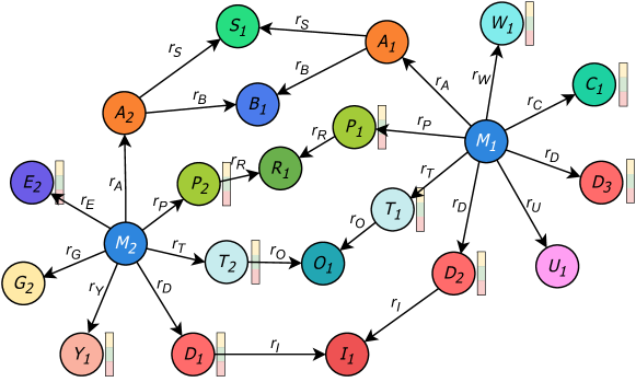
Figure 1: An example of a sub-graph from our knowledge graph. The circles and the rectangles surrounding entities denote entities and their attributes, respectively. Several entities, such as $M$, $A$, $R$, $O$, and $D$, denote the Medical records, Animals, Drugs, Treatment code, and Disease, respectively.

We now represent our strategy to construct a medical knowledge graph from EMRs. A knowledge graph (KG) is a semantic network that represents heterogeneous data with different types of entities and relations in the real world [32, 33]. Formally, a KG is a set of triples where each triple is formed of $\langle h,r,t\rangle$, where $h,r,t$ refers to the head, relation, and tail, respectively [45]. Medical knowledge graph (MKG) is a knowledge graph that represents the relations in the healthcare area through representing medical data, i.e., electronic medical records (EMRs) [4]. These records contain various types of information, such as patients, diseases, medicines, and symptoms [46, 4].

We now explain our proposed strategy to construct a KG and entity relations from EMRs. In our study, we constructed a KG, which is composed of 85,965 EMRs from 31 companion animal hospitals, collected from IntoCNS company. In EMRs, a record is a collection of medical properties, such as companion animal, symptoms, disease, and the veterinarian’s decisions for each companion animal visit. We generate entities from the medical properties. There are a total of sixteen entity types and fifteen relation types in our KG. Table 1 shows the detailed statistics of entity types and their relations. In each record, the types and names of the entities are extracted from the fields and elements in EMRs, respectively.

Figure 1 illustrates simplified entities and their relations in our MKG. Our purpose is first to construct entities and then build different types of relations between entities in KGs from EMRs. Let $\mathbb{M}$ denote the set of medical record entities, and $\mathbb{A}$ refers to the animal entity set. We construct one-to-many relations between animal entity $\mathbb{A}$ and $\mathbb{M}$ since an animal $A_{i}$ could be examined many times and have more thane one medical record. Other entities in our MKG are constructed into a structure that satisfies their natural types of relations. For example, the relations between $\mathbb{M}$ and $\mathbb{D}$ are many-to-many since one animal could suffer many diseases or many animals have the same diseases.

Note that the entities are composed of different types of attributes, such as numeric and text attributes. For example, the disease, symptom, treatment, age, and weight entities have textual or numerical attributes that can be divided into numeric or text groups. For textual attributes, we then encode the attributes by using Fasttext [47] to capture the semantic contexts of the textual attributes. Otherwise, if an entity does not contain an attribute, its attribute embedding should be known as a non-attribute entity. In this case, the textual or numerical attribute vectors will be presented as vectors of zero. Accordingly, we then fuse entity and attributed features through gate networks to generate literal enriched embedding vectors for entities.

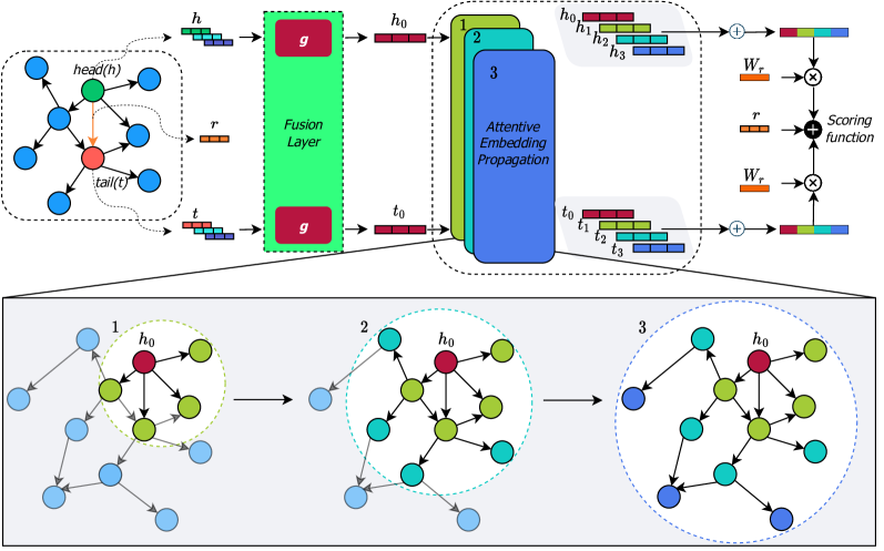
Figure 2: The overall architecture of LiteralKG. The entities and attributes are fused into unified vectors through a gate function $g(\cdot)$. The unified vectors are then passed through attentive embedding propagation layers to generate the output representations. The output representations are then concatenated with the initial embeddings to generate final representations by optimizing a score function.

4 Literal-aware Medical Knowledge Graph Representation Learning

In this section, we first represent how to fuse entities and different attribute types into unified representations. Then, we will introduce the architecture of our model in detail. In addition, we represent a pre-training task that could learn the representations in the pretext tasks and then apply them to downstream tasks, i.e., predicting diseases.

4.1 Fusing Entity and Attribute Features

As mentioned earlier, the entities contain two main types of attributes, including numerical and textual attributes. We first design a fusion layer that contains a gate function to transform different types of attributes into unified vectors. The textual attributes, such as disease, symptom, prescription, treatment, and comment, are transformed into vectors through Fasttext [47]. Numerical attributes, such as age and weight entities, are normalized and transformed directly into feature vectors [19]. In several cases, missing values are represented by ‘-1’ as missing features. We then linearly transform entities into the shared space to generate the unified literal-enriched vectors by using a gate function [19]. Formally, the output representations for an $i$-th entity can be defined as:

$$h_{i}^{(0)}=g(e_{i},n_{i},t_{i})=\mu\odot\nu+(1-\mu)\odot e_{i}\ ,$$ (1)

where, $$\mu=\sigma_{1}\left(W_{E}\cdot e_{i}+W_{N}\cdot n_{i}+W_{T}\cdot t_{i}+b\right),\ \nu=\sigma_{2}\left(W\cdot\left({e_{i}\|n_{i}\|t_{i}}\right)\right),$$

and $\odot$ is the Hadamard product, $\sigma_{1}$ and $\sigma_{2}$ are sigmoid and tanh activation functions, respectively. The entity vector $e_{i}\in\mathbb{R}^{E}$ , the numerical attribute vector $n_{i}\in\mathbb{R}^{N}$ and the textual attribute vector $t_{i}\in\mathbb{R}^{T}$ are combined and transformed into a vector $h_{i}^{(0)}\in\mathbb{R}^{h}$ with fixed dimension $h$ by a gate function $g$. $W_{E}\in\mathbb{R}^{E\times h}$, $W_{N}\in\mathbb{R}^{N\times h}$, $W_{T}\in\mathbb{R}^{T\times h}$ and $b\in\mathbb{R}^{h}$ and $W\in\mathbb{R}^{(E+N+T)\times h}$ are learnable parameters.

4.2 Learning Global and Local Structural Features

After generating literal-enriched embedding vectors, we use an attention mechanism to learn the co-coefficients across triplets. Figure 2 shows the overall architecture of our model. The literal-enriched embedding vectors will be passed through the attentive embedding propagation layers. Formally, the representation of a entity $e_{i}$ at $l$-th layer could be updated as:

$$h^{(l)}_{i}= \text{ }f_{*}{\left(h_{i}^{(l-1)},h_{\mathcal{N}_{i}}^{(l-1)}\right)}\ ,$$ (2)

$$h_{\mathcal{N}_{i}}^{(l-1)}= \sum_{\forall{(h_{i},r_{j},t_{k})}\in\mathcal{N}_{i}}\pi(h_{i},r_{j},t_{k})t_{k}^{(l-1)}\ ,$$ (3)

where $h^{(l)}_{i}$ is the output representation of an entity $e_{i}$ at $l$-th layer, $\mathcal{N}_{i}$ denotes a set of neighbours of entity $e_{i}$ which is composed with the triple $(h_{i},r_{j},t_{k})$ if and only if there is a link between $h_{i}$ and $t_{k}$, and $f_{*}$ is a GNN aggregator.

Since neighbours with different relation types could contribute differently to a target entity, we aim to aggregate features of neighbouring nodes with attentional weights to benefit the model in learning different relations between entities. The attentive weights could, therefore, describe the nature of the relations between entities in KGs. More formally, the attentive scores are computed as follows:

$$\pi(h,r,t) =(W\cdot t)^{\intercal}\tanh(W\cdot h+r)\ ,$$ (4)

$$\pi(h,r,t) :=\frac{exp(\pi(h,r,t))}{\sum_{{(h,r^{{}^{\prime}},t^{{}^{\prime}})\in\mathcal{N}_{i}}}exp(\pi(h,r^{{}^{\prime}},t^{{}^{\prime}}))}\ .$$ (5)

Since different GNN aggregators show individual characteristics, they could benefit in different ways to explore the explicit and complex KG structures. Therefore, we aim to investigate which types of GNN aggregators could contribute to the overall performance of our model. In this study, we use four aggregators, including GCN, GraphSAGE, Bi-Interaction, and GIN aggregators. First, GCN aggregator [48] combines the entity feature and its neighbour’s features by a sum operator. At each $k$-th layer, the model aggregates $k$-hop neighbourhood features to leverage the graph structure and generate output representation. A non-linearity transformation is then utilized to transform the output features before updating the representations. The GCN aggregator is defined as:

$$f_{GCN}^{(l)}{\left(h_{i}^{(l-1)},h_{\mathcal{N}_{i}}^{(l-1)}\right)}=\sigma\left(W^{(l)}\left(h_{i}^{(l-1)}+h_{\mathcal{N}_{i}}^{(l)}\right)\right)\ ,$$ (6)

where $\sigma$ denotes the activation function, $h_{i}^{(l-1)}$ and $h_{\mathcal{N}_{i}}^{(l-1)}$ are the output of the previous layer and the aggregated neighbourhood features of an entity, respectively, and $W^{(l)}$ is the learnable transformation matrix at $l$-th layer.

GraphSAGE aggregator replaces sum by concatenation operator to distinguish between the entity feature and its neighbourhood aggregation feature [49, 48]. Note that the difference between GCN and GraphSAGE is that GraphSAGE learns the topological structure for each target node neighbourhood through random walks, which could then calculate node embeddings in an inductive manner. GraphSAGE aggregator is described as follows:

$$f_{SAGE}^{(l)}{\left(h_{i}^{(l-1)},h_{\mathcal{N}_{i}}^{(l-1)}\right)}=\sigma\left(W^{(l)}\left(h_{i}^{(l-1)}\|h_{\mathcal{N}_{i}}^{(l-1)}\right)\right)\ ,$$ (7)

where $\|$ is the concatenation.

Wang et al. [48] have proposed a Bi-Interaction aggregator which combines the GCN-based strategy and the element-wise product of the target node and its neighbour feature. The element-wise product could assist the model in learning the similarity between target nodes and neighbourhoods. Formally, the Bi-Interaction equation is considered as follows:

$$f_{BI}^{(l)}{\left(h_{i}^{(l-1)},h_{\mathcal{N}_{i}}^{(l-1)}\right)}=\sigma\left(W_{1}^{(l)}\left(h_{i}^{(l-1)}+h_{\mathcal{N}_{i}}^{(l-1)}\right)\right)+\sigma\left(W_{2}^{(l)}\left(h_{i}^{(l-1)}\odot h_{\mathcal{N}_{i}}^{(l-1)}\right)\right)\ ,$$

where $W_{1}^{(l)}$ and $W_{2}^{(l)}$ are the learnable parameters.

Inspired by 1-d Weisfeiler-Lehman (WL) isomorphism testing, GIN [50] aims to maximize the GNNs power up to $1$d-WL test. The key difference between GIN and other aggregators is that GIN could map different sub-structures into different representations, leading to the power to distinguish non-isomorphic sub-structures. At each layer, the GIN aggregator updates the representations through the entity and neighbour features with a sum aggregator. Note that GIN does not include any normalization during updating node features. The GIN aggregator can be described as:

$$f_{GIN}^{(l)}{\left(h_{i}^{(l-1)},h_{\mathcal{N}_{i}}^{(l-1)}\right)} =\sigma\left[FC\left(\left(1+\epsilon^{(l)}\right)\cdot h_{i}^{(l-1)}+h_{\mathcal{N}_{i}}^{(l-1)}\right)\right],$$

where $\epsilon$ can be a fixed scale or learnable parameter, and $FC$ denotes the fully connected layer.

Stacking more GNN layers can lead to the over-smoothing problem, and eventually lead to reducing the performance of the model. Therefore, we add initial residual connections and identity mapping, following the work [20]. Formally, the formula of residual connection and identity mapping can be described as:

$$H^{(l+1)}= \sigma\left[\left((1-\alpha_{l})\tilde{P}H_{i}^{(l)}+\alpha_{l}H_{i}^{(0)}\right)\left((1-\beta_{l})I_{n}+\beta_{l}W^{(l)}\right)\right],$$ (9)

where $\beta_{l}=\log{\frac{\lambda}{1+l}}$, $\tilde{P}=(D+I_{n})^{-1/2}(A+I_{n})(D+I_{n})^{-1/2}$, and $\tilde{P}$ is a graph convolution matrix, $\lambda$ and $\alpha_{l}$ are hyper-parameters.

To compute the final representation of an $i$-th entity $e_{i}$, we first concatenate all the output representations of GNN layers. As the local and global graph structures are important to represent entities, we aim to combine the initial feature with the output features of all GNN layers. Therefore, the representations could learn the local and global graph structures [48, 11]. We then apply a linear function followed by an activation function to transform the entity vectors into final representations:

$$e_{i}=\sigma\left(W\cdot\operatorname*{\mathchoice{\Big{\|}}{\big{\|}}{\|}{\|}}_{k=1}^{K}\left(h_{i}^{(k)}\right)+b\right),$$ (10)

where $K$ presents the number of GNN layers, ${b}$ is the bias of the linear function, and $W\in\mathbb{R}^{h\times K}\rightarrow{\mathbb{R}}^{d}$ is the weight matrix.

4.3 Pre-training with Focusing on Multi-relational Structures

We now represent our pre-training task to learn multi-relational structures between different types of entities in KG. In this study, we aim to preserve the triplet relations using a translation-based method. For each triplet, entity embedding vectors are first transformed to a shared space through a projection matrix. Then, we use a triplet score function to calculate their relation score [33]. To preserve all the entity relations, we aim to maximize all the positive triplets coming from KGs and minimize all the negative triplets that are not coming from KGs [32, 33]. Formally, the scoring function is defined as:

$$f_{score}=\hat{y}(h,r,t)=W_{r}h+r-W_{r}t\ ,$$ (11)

where $h$, $t$, and $r$ are the output representations of head, tail, and relation, and $W_{r}$ is a projection matrix to map entities and relations onto the $r$ space. A triplet loss function is computed to compare the positive and negative triple pairs defined as:

$$\mathcal{L}_{\mathcal{P}}(\mathcal{T})=\sum_{\forall(h,r,t)\in\mathcal{T}} -{\ln\sigma\left(\hat{y}(h,r,\bar{t})-\hat{y}(h,r,t)\right)}+\lambda||\Theta||_{2}^{2},$$

where $\mathcal{T}$ denotes the set of triplets, $(h,r,\bar{t})$ denote the negative triplet, $\Theta$ refers to $L_{2}$ regularization parameter.

4.4 Fine-tuning for Animal Disease Diagnostics

We now apply learned LiteralKG and representations to new downstream task, such as predicting animal diseases. We first compute a coefficient score to measure the relationship between each head and tail pair. The equation for calculating the coefficient score can be formulated as follows:

$$\hat{y}_{h,t}=\hat{y}(h,t)=\langle\phi(h),\phi(t)\rangle\ =FC(W_{r}h||W_{r}t),$$ (13)

where $h$ and $t$ denote the learned representations of head and tail, respectively, $||$ is the concatenation operator, $W_{r}$ is the transformation matrix corresponding to the relation between $h$ and $t$, and $FC$ denotes the fully connected layers to get the prediction output.

For disease diagnosis, the model classifies the coefficient score between two entities into binary digits. With pre-trained embeddings, two observed entity vectors are first projected into the relation space. Their embedding vectors are then concatenated and transformed into a one-dimensional class by MLP layers to form the coefficient score. It is used to identify the relationship probability among the observed entities. Additionally, a binary cross entropy loss function is utilized for training classification. The loss function is described as:

$$\mathcal{L}_{\mathcal{F}}(\mathcal{M})= -\sum_{\forall(M_{k},D_{i})\in\mathcal{M}}\left[y_{M_{k},D_{i}}\log\left(\hat{y}_{M_{k},D_{i}}\right)+(1-y_{M_{k},D_{i}})\log\left((1-\hat{y}_{M_{k},D_{i}})\right)\right]\ ,$$ (14)

where $M_{k}$ and $D_{i}$ are the medical record and disease entity, $y_{M_{k},D_{i}}$ and $\hat{y}_{M_{k},D_{i}}$ are the actual and predicted outputs, and $\mathcal{M}$ is the collection of all the training medical records containing positive and negative disease information.

5 Experiments

In this section, we provide extensive experimental results to validate the performance of our model versus baselines. In addition, we conduct ablation studies to investigate the contribution of the combination of different types of relations as well as residual connection and identity mapping to the overall performance.

5.1 Experimental Settings

5.1.1 Dataset Description

As mentioned earlier, we collected 85,965 EMRs from 31 animal hospitals and transformed to a knowledge graph. After transforming, our MKG contains a total of 595,172 entities and 16 relation types. Note that we sampled three negative triplets for each positive triplet in the experiments. We first pre-trained our model in a self-supervised manner without using any label information. Then, we fine-tuned the LiteralKG model to learn the knowledge for link prediction tasks. For the fine-tuning task, we conducted the experiment by randomly sampling training, validation, and testing sets of size 60%, 20%, and 20%, respectively.

5.1.2 Evaluation Metrics

Since our task is a binary classification problem, we utilized several evaluation metrics, including accuracy ($Acc$), precision ($P$), recall ($R$), and $F_{1}$. The evaluation metrics are defined as follows:

$$Acc=\frac{|D^{+}_{true}\cup D^{-}_{true}|}{|D^{+}\cup D^{-}|}\ ,\ P=\frac{|D^{+}_{true}|}{|D^{+}|}\ ,R=\frac{|D^{+}_{true}|}{|D^{+}_{true}\cup D^{-}_{false}|}\ ,\ F_{1}=2\frac{(PR)}{(P+R)}\ ,$$ (15)

where the $D^{+}_{true}$ and $D^{-}_{true}$ denote the correct predictions for positive and negative diseases, respectively, and $D^{-}_{false}$ is the incorrect predictions for negative diseases. These criteria are intended to assess how well our model performs compared to baselines.

5.1.3 Baselines

We compare our model to relevant translation-based methods and GNN models, which have gained remarkable success in KG representation learning. Translation-based models learn representations by mapping the entities and their relations into latent space through translations from head-to-tail entities.

• TransE [32]. The model uses a simple scoring function to compare the relationships between the pairs of entities. Note that all types of entities and relations are represented in the same space.

• TransR [33]. TransR uses projection matrices to map various types of entities into different relation spaces and then construct translations between entities.

• SMR [4]. The idea of SMR is to use TransR to transform entities into latent space linearly. Meanwhile, SMR uses the LINE [51] model to capture the similarity between entities, which successfully addresses homogeneous graphs.

Furthermore, we also compare our model with recent GNNs, which could learn high-order sub-structures and semantic relations in KGs. There are three GNN baselines, including KGNN, KGNMDA, and LaGAT model, as:

• KGNN [10] learn KG structures through a local receptive to aggregate neighbour features and topological information. KGNN could also capture the high-order structures surrounding target entities and semantic relations to learn global structural information.

• KGNMDA [52] represent the relations between microbes and diseases based on the Gaussian kernel and then learn the similarity between them in an uncertain manner. They then use a linear transformation to predict the scores across microbe-disease relations.

• LaGAT [11] extends KGNN by using an attentive mechanism, which could learn different weighted messages contributed from different entities. Furthermore, the outputs of different attentive embedding propagation layers are concatenated and then contribute to the final representations.

5.1.4 Implementation Details

Our model is implemented based on the Pytorch library. Adam optimizer [53] was applied to the pre-training and fine-tuning phases. We applied Leaky ReLU as an activation function in the aggregation layers. Additionally, the dimensions of entity and relation vectors were set to 300. We initialized the learning rate at 0.0001. Referred to current GNN hyper-parameter settings [54, 49, 50, 48], the tuning hyper-parameters are: (1) the hidden dimension of the GNN layer $\in\{16,32\}$, (2) the batch size for the pre-training and fine-tuning phases $\in\{1024,2048\}$, (3) the number of GNN layer $\in\{2,4,8,16\}$, and (4) the dropout ratio $\in\{0.1,0.5\}$ after each layer. The number of layers in various GNN models was tuned to evaluate the performance of these models and the effectiveness of applying residual connection in MKG. For fair comparisons with the baselines, the hyper-parameters in all baselines were tuned in the same range, including the learning rate $\in\{0.001,0.0001\}$, hidden dimension $\in\{16,32,64,128\}$ and the number of layers $\in\{1,2,4\}$.

5.2 Performance Analysis

Table 3: The performance of LiteralKG and baselines in terms of accuracy, recall, precision and $F_{1}$. The top two are highlighted by first and second.

Model	Accuracy	Recall	Precision	$F_{1}$
TransE [32]	0.5937	0.5617	0.6001	0.5802
TransR [33]	0.5732	0.5915	0.5706	0.5808
SMR [4]	0.5872	0.5669	0.5909	0.5787
KGNN [10]	0.7890	0.7021	0.8499	0.7689
KGNMDA [52]	0.8130	0.7111	0.8932	0.7918
LaGAT [11]	0.8545	0.7988	0.8988	0.8459
LiteralKG	0.8616	0.9357	0.8150	0.8712

Table 3 shows the performance of our model and baselines in terms of accuracy, recall, precision, and $F_{1}$. We have the following observations: (1) LiteralKG with pre-training outperformed baselines in most measurements. Specifically, our proposed model reached the best value at $0.9357$ regarding Recall measurement. We argue that our model could learn the literal information well to maximize the relations between entities. (2) Translation-based models, i.e., TransE, TransR, and SMR, showed low performance in predicting disease. We argue that these models overlooked literal information and eventually could not capture the complex relations since they only learn representations through simple linear transformations. (3) LaGAT showed competitive performance compared to our model. We argue that as LaGAT could learn graph structure through the attention mechanism, the model thus could learn attentive weights contributed from different neighbourhood entities in KGs.

5.3 Ablation Studies

Table 4: The results for evaluating the efficiency of leveraging literals. The first column contains the combining literal strategies. There are four cases, including without (w/o) literal, without textual, without numerical, and the combination of numerical and textual features. The top two are highlighted by first and second.

Combining literals	Accuracy	Recall	Precision	$\textbf{F}_{1}$
w/o  literal	0.8223	0.8664	0.7962	0.8298
w/o  textual	0.8424	0.8544	0.8344	0.8443
w/o  numerical	0.8529	0.9116	0.8158	0.8610
numerical $+$ textual	0.8616	0.9357	0.8150	0.8712

5.3.1 On the Importance of Learning Literal Information

Table 4 shows how the literal information contributes to the overall performance of our model. We have the following observations: (1) LiteralKG showed the best performance with the combination of numerical and textual information in most measurements. We argue that both types of literal information could benefit our model to explore similar entities in the KG and thus contribute to the overall performance. (2) We find out that without numerical information, the performance of our model increased slightly, from 0.8529 to 0.8616 and from 0.8610 to 0.8712 in terms of accuracy and $F_{1}$, respectively. It indicates that the textual information contributes considerably to the overall performance compared to numerical attributes. Thanks to the textual features, LiteralKG performs well even without numerical features. (3) When combining different types of attributes, the recall measurement increased from 0.8664 to 0.9357, which shows a good point for maximizing the ability to diagnose patients with a correct disease. It indicates that the gating mechanism transformed the attributes and entity embedding vectors into the shared space and eventually contributed to the overall performance.

Table 5: Link prediction performance on the Residual Connection and Identity Mapping (R.C& I.M) in GNN aggregators. $\times$ and $\bigcirc$ denote a setting ignoring and adopting residual connection, respectively. The top two are highlighted by first and second.

R.C& I.M	Aggregator	Accuracy	Recall	Precision	$\textbf{F}_{1}$
$\times$	GCN	0.8532	0.9419	0.8000	0.8652
	GraphSAGE	0.8580	0.9257	0.8154	0.8670
	Bi-Interaction	0.8545	0.9123	0.8178	0.8625
	GIN	0.8387	0.8621	0.8236	0.8424
$\bigcirc$	GCN	0.8527	0.9170	0.8125	0.8616
	GraphSAGE	0.8300	0.8882	0.7956	0.8394
	Bi-Interaction	0.8616	0.9357	0.8150	0.8712
	GIN	0.8490	0.9372	0.7967	0.8612

Table 6: The performance of LiteralKG on the role of the pre-training task. $\times$ and $\bigcirc$ denote a setting without a pre-trained model and utilizing the pre-trained model, respectively. The top two are highlighted by first and second.

Pre-training	Aggregator	Accuracy	Recall	Precision	$\textbf{F}_{1}$
$\times$	GCN	0.8183	0.7371	0.8801	0.8022
	GraphSAGE	0.8109	0.7429	0.8597	0.7971
	Bi-Interaction	0.7976	0.7083	0.8622	0.7777
	GIN	0.8013	0.8053	0.7989	0.8021
$\bigcirc$	GCN	0.8527	0.9170	0.8125	0.8616
	GraphSAGE	0.8300	0.8882	0.7956	0.8394
	Bi-Interaction	0.8616	0.9357	0.8150	0.8712
	GIN	0.8490	0.9372	0.7967	0.8612

5.3.2 On the Importance of Residual Connection and Identity Mapping

We further conducted experiments to evaluate the effectiveness of residual connection and identity mapping shown in Table 5. We have the following observations: (1) The overall performance increased slightly by applying the residual connection and identity mapping. It indicates that even though KGs have complex relations and heterophily properties, residual connections and identity mapping could act as auxiliary modules to contribute to the overall performance of LiteralKG. In other words, the two modules could help LiteralKG prevent over-smoothing problem and improve the performance of our model. (2) In comparison with GraphSAGE, the performance of our model with residual connection has been reduced from 0.8580 to 0.8300 and from 0.8670 to 0.8394 in terms of accuracy and $F_{1}$, respectively. It indicates that the residual connection does not contribute much to our model performance as GraphSAGE sampled the neighbourhoods based on random walks. (3) For the GIN aggregator, using residual connection can improve the model performance from 0.8174 to 0.8378 in terms of $F_{1}$ measure. Note that GIN aggregators aim to map different sub-structures into different representations, leading to the power of 1d-WL isomorphism testing. This implies that residual connections could contribute to the model performance as GIN aggregators could ignore the original features of entities.

Figure 3: Performance on link prediction over attentive embedding propagation layers on four types of aggregators, including GCN, GraphSAGE, Bi-Interaction, and GIN aggregators.

5.3.3 On the Pre-training Phase

Table 6 shows the link prediction performance on the pre-training phase evaluation. We discovered that our pre-trained model could show comparable performance in most of the aggregators. In particular, LiteralKG reaches the highest values in the Bi-Interaction aggregator at 0.8616, 0.8150, and 0.8712 in terms of accuracy, precision, and $F_{1}$, respectively. We argue that the triplet scoring function in the pre-training phase first learns to maximize relation proximity among entities in correct triplets. Therefore, it improves the performance of the fine-tuning model in link prediction, in which the link is also considered by representation proximity. In GIN, applying the pre-trained model improves performance on $F_{1}$ and accuracy from 0.8021 to 0.8612 and 0.8013 to 0.8490, respectively. These results, therefore, explain the efficiency of the pre-trained model, which satisfies the RQ2.

5.4 Sensitivity Analysis

Figure 3 shows the performance of our model by applying different range of GNN layers. We have the following observations: (1) This result illustrates that LiteralKG with a $1$-layer or $2$-layer can efficiently learn the KG structure in most of the aggregators. For the Bi-Interaction aggregator, LiteralKG achieves the best performance when using only one layer, which captures 1-hop neighbourhood entities. We argue that as Bi-Interaction could capture the graph structure through sum aggregators and element- wise product, the aggregators could suffer the over-smoothing problem when staking more layers. In other words, Bi-Interaction aggregators could not distinguish sub-structures as the aggregators learned the similarity between target nodes and neighbours at the first layers. (2) It is worth noting that GIN aggregators show the best performance when staking more GNN layers compared to other aggregators. We argue that as the power of GIN achieves nearly 1d-WL isomorphism testing, the model then could handle the over-smoothing problem even staking more GNN layers. In other words, GIN aggregators could distinguish different sub-structures even staking more layers.

6 Conclusion and Future Work

In this study, we propose a knowledge graph embedding model, LiteralKG, which could learn different types of entity attributes to diagnose companion animal disease. By doing so, we first constructed an MKG from various EMRs collected from 31 animal hospitals. Then, LiteralKG fuses different types of literals into unified representations through a gating network. We then use the attention mechanism with the initial feature to learn the coefficients across triplets to capture local and global graph structures. The experiment results show that our model outperforms the shallow KG embedding and GNN-based models due to the improvements from leveraging the literal features and the efficiency of the pre-trained phase. Furthermore, we present a pre-training task that could learn graph structure and its properties without using any label information to generate learned representations. The pre-trained model with representations could then be used for prediction tasks. Besides, the negative samples from our data are sampled randomly so that it can affect the overall performance of LiteralKG. In future work, we plan to build useful sampling strategies to effectively build positive and negative samples, such as graph clustering and sub-graph sampling methods.

References

- [1] Yuhui Zhang, Allen Nie, Ashley Zehnder, Rodney López Page, and James Zou. Vettag: improving automated veterinary diagnosis coding via large-scale language modeling. NPJ digital medicine, 2, 2019.
- [2] Mary Regina Boland, Margret L Casal, Marc S Kraus, and Anna R Gelzer. Applied veterinary informatics: development of a semantic and domain-specific method to construct a canine data repository. Scientific reports, 9(1):1–13, 2019.
- [3] Sandra Valéria Inácio, Jancarlo Ferreira Gomes, Alexandre Xavier Falcão, Celso Tetsuo Nagase Suzuki, Walter Bertequini Nagata, Saulo Hudson Nery Loiola, Bianca Martins dos Santos, Felipe Augusto Soares, Stefani Laryssa Rosa, Carolina Beatriz Baptista, et al. Automated diagnosis of canine gastrointestinal parasites using image analysis. Pathogens, 9(2):139, 2020.
- [4] Fan Gong, Meng Wang, Haofen Wang, Sen Wang, and Mengyue Liu. SMR: medical knowledge graph embedding for safe medicine recommendation. Big Data Research, 23:100174, 2021.
- [5] Meng Gao, Haodong Wang, Weizheng Shen, Zhongbin Su, Huihuan Liu, Yanling Yin, Yonggen Zhang, and Yi Zhang. Disease diagnosis of dairy cow by deep learning based on knowledge graph and transfer learning. International Journal Bioautomation, 25(1):87, 2021.
- [6] Ashley N Paynter, Matthew D Dunbar, Kate E Creevy, and Audrey Ruple. Veterinary big data: when data goes to the dogs. Animals, 11(7):1872, 2021.
- [7] Jin Li, Jing Gao, Baiyang Feng, and Yi Jing. Plaguekd: a knowledge graph-based plague knowledge database. The journal of biological databases and curation, Nov 2022.
- [8] Lino Murali, G Gopakumar, Daleesha M Viswanathan, and Prema Nedungadi. Towards electronic health record-based medical knowledge graph construction, completion, and applications: A literature study. Journal of Biomedical Informatics, page 104403, 2023.
- [9] Linfeng Li, Peng Wang, Yao Wang, Shenghui Wang, Jun Yan, Jinpeng Jiang, Buzhou Tang, Chengliang Wang, Yuting Liu, et al. A method to learn embedding of a probabilistic medical knowledge graph: algorithm development. JMIR medical informatics, 8:e17645, 2020.
- [10] Xuan Lin, Zhe Quan, Zhi-Jie Wang, Tengfei Ma, and Xiangxiang Zeng. KGNN: knowledge graph neural network for drug-drug interaction prediction. In Proceedings of the 29th International Joint Conference on Artificial Intelligence (IJCAI 2020), volume 380, pages 2739–2745, Yokohama, Japan, Jul. 11–17, 2020. ijcai.org.
- [11] Yue Hong, Pengyu Luo, Shuting Jin, and Xiangrong Liu. Lagat: link-aware graph attention network for drug-drug interaction prediction. Bioinformatics, 38(24):5406–5412, 2022.
- [12] Chutchada Nusai, Sirisak Cheechang, Somkid Chaiphech, and Goragot Thanimkan. Swine-vet: a web-based expert system of swine disease diagnosis. Procedia computer science, 63:366–375, 2015.
- [13] Ariadi Nugroho et al. Mobile expert system using fuzzy tsukamoto for diagnosing cattle disease. Procedia computer science, 116:27–36, 2017.
- [14] Xuqing Chai. Diagnosis method of thyroid disease combining knowledge graph and deep learning. IEEE Access, 8:149787–149795, 2020.
- [15] Wei Lan, Yi Dong, Qingfeng Chen, Ruiqing Zheng, Jin Liu, Yi Pan, and Yi-Ping Phoebe Chen. KGANCDA: predicting circrna-disease associations based on knowledge graph attention network. Briefings Bioinform., 23(1), 2022.
- [16] Xiao Xu, Xian Xu, Yuyao Sun, Xiaoshuang Liu, Xiang Li, Guotong Xie, and Fei Wang. Predictive modeling of clinical events with mutual enhancement between longitudinal patient records and medical knowledge graph. In Proceedings of the 21st International Conference on Data Mining (ICDM 2021), pages 777–786, Auckland, New Zealand, Dec. 7–10, 2021. IEEE.
- [17] Zachary C Lipton, David C Kale, Charles Elkan, and Randall Wetzel. Learning to diagnose with lstm recurrent neural networks. arXiv preprint, arXiv:1511.03677, 2015.
- [18] Van Thuy Hoang and O-Joun Lee. Transitivity-preserving graph representation learning for bridging local connectivity and role-based similarity. arXiv preprint, arXiv:2308.09517, 2023.
- [19] Agustinus Kristiadi, Mohammad Asif Khan, Denis Lukovnikov, Jens Lehmann, and Asja Fischer. Incorporating literals into knowledge graph embeddings. In Proceedings of the 18th International Semantic Web Conference (ISWC 2019), volume 11778 of Lecture Notes in Computer Science, pages 347–363, Auckland, New Zealand, Oct. 26–30, 2019. Springer.
- [20] Ming Chen, Zhewei Wei, Zengfeng Huang, Bolin Ding, and Yaliang Li. Simple and deep graph convolutional networks. In Proceedings of the 37th International Conference on Machine Learning (ICML 2020, volume 119 of Proceedings of Machine Learning Research, pages 1725–1735, Virtual Event, Jul. 13–18, 2020. PMLR.
- [21] Van Thuy Hoang , Hyeon-Ju Jeon , Eun-Soon You , Yoewon Yoon , Sungyeop Jung , and O-Joun Lee . Graph representation learning and its applications: A survey. Sensors, 23(8), 2023.
- [22] Petar Veličković, Guillem Cucurull, Arantxa Casanova, Adriana Romero, Pietro Liò, and Yoshua Bengio. Graph Attention Networks. International Conference on Learning Representations, 2018.
- [23] Hyeon-Ju Jeon, Gyu-Sik Choi, Se-Young Cho, Hanbin Lee, Hee Yeon Ko, Jason J Jung, O-Joun Lee, and Myeong-Yeon Yi. Learning contextual representations of citations via graph transformer. In Proceeding of the 2nd International Conference on Human-centered Artificial Intelligence (Computing4Human 2021), Da Nang, Vietnam, Oct. 2021.
- [24] Thanh Sang Nguyen, Jooho Lee, Van Thuy Hoang, and O-Joun Lee. Connector 0.5: A unified framework for graph representation learning. arXiv preprint, arXiv:2304.13195, 2023.
- [25] Hyeon-Ju Jeon, Min-Woo Choi, and O-Joun Lee. Day-ahead hourly solar irradiance forecasting based on multi-attributed spatio-temporal graph convolutional network. Sensors, 22(19):7179, Sep. 2022.
- [26] Jiawei Zhang, Haopeng Zhang, Congying Xia, and Li Sun. Graph-bert: Only attention is needed for learning graph representations. arXiv preprint, arXiv:2001.05140, 2020.
- [27] Yunsang Joo, Hyun-Cheol Park, O-Joun Lee, Changhan Yoon, Moon Hyung Choi, and Chang Choi. Classification of liver fibrosis from heterogeneous ultrasound image. IEEE Access, 11:9920–9930, 2023.
- [28] Chao Zhao, Jingchi Jiang, Yi Guan, Xitong Guo, and Bin He. Emr-based medical knowledge representation and inference via markov random fields and distributed representation learning. Artificial intelligence in medicine, 87:49–59, 2018.
- [29] O-Joun Lee and Jason J. Jung. Story embedding: Learning distributed representations of stories based on character networks (extended abstract). In Proceedings of the 29th International Joint Conference on Artificial Intelligence (IJCAI 2020), pages 5070–5074. ijcai.org, Sep. 05, 2020.
- [30] O-Joun Lee and Jason J. Jung. Story embedding: Learning distributed representations of stories based on character networks. Artificial Intelligence, 281:103235, 2020.
- [31] O-Joun Lee, Sung Youn Park, and Jin-Taek Kim. Ideanet: Potential opportunity discovery for business innovation. In Proceedings of AI4Narratives - Workshop on Artificial Intelligence for Narratives in conjunction, volume 2794 of CEUR Workshop Proceedings, pages 5–8, Yokohama, Japan, Jan. 07–08, 2020. CEUR-WS.org.
- [32] Antoine Bordes, Nicolas Usunier, Alberto García-Durán, Jason Weston, and Oksana Yakhnenko. Translating embeddings for modeling multi-relational data. In Proceedings of the 27th Annual Conference on Neural Information Processing Systems (NeurIPS 2013), volume 26, pages 2787–2795, Lake Tahoe, Nevada, United States, Dec. 05–08, 2013.
- [33] Yankai Lin, Zhiyuan Liu, Maosong Sun, Yang Liu, and Xuan Zhu. Learning entity and relation embeddings for knowledge graph completion. In Proceedings of the 29th Conference on Artificial Intelligence (AAAI 2015), pages 2181–2187, Austin, Texas, USA, Jan. 25–30 2015. AAAI Press.
- [34] Zhen Wang, Jianwen Zhang, Jianlin Feng, and Zheng Chen. Knowledge graph embedding by translating on hyperplanes. In Proceedings of the 28th AAAI Conference on Artificial Intelligence (AAAI 2014), volume 28, pages 1112–1119, Québec City, Québec, Canada, Jul. 27–31, 2014. AAAI Press.
- [35] Guoliang Ji, Shizhu He, Liheng Xu, Kang Liu, and Jun Zhao. Knowledge graph embedding via dynamic mapping matrix. In Proceedings of the 53rd Annual Meeting of the Association for Computational Linguistics (ACL 2015), pages 687–696, Beijing, China, Jul. 26–31, 2015. ACL.
- [36] Guoliang Ji, Kang Liu, Shizhu He, and Jun Zhao. Knowledge graph completion with adaptive sparse transfer matrix. In Proceedings of the 30th Conference on Artificial Intelligence (AAAI 2016), pages 985–991, Phoenix, Arizona, USA, Feb. 12–17, 2016. AAAI Press.
- [37] Tim Dettmers, Pasquale Minervini, Pontus Stenetorp, and Sebastian Riedel. Convolutional 2d knowledge graph embeddings. In Proceedings of the 32nd Conference on Artificial Intelligence (AAAI 2018), pages 1811–1818, New Orleans, Louisiana, USA, Feb. 2–7, 2018. AAAI Press.
- [38] Hyeon-Ju Jeon, O-Joun Lee, and Jason J. Jung. Is performance of scholars correlated to their research collaboration patterns? Frontiers Big Data, 2:39, 2019.
- [39] Yi Tay, Luu Anh Tuan, Minh C. Phan, and Siu Cheung Hui. Multi-task neural network for non-discrete attribute prediction in knowledge graphs. In Proceedings of the 2017 on Conference on Information and Knowledge Management (CIKM 2017), pages 1029–1038, Singapore, Nov. 06–10, 2017. ACM.
- [40] Yanrong Wu and Zhichun Wang. Knowledge graph embedding with numeric attributes of entities. In Proceedings of the 3rd Workshop on Representation Learning for NLP(Rep4NLP@ACL 2018), pages 132–136, Melbourne, Australia, Jul. 20, 2018. ACL.
- [41] Yancong Li, Xiaoming Zhang, Fang Wang, Bo Zhang, and Feiran Huang. Fusing visual and textual content for knowledge graph embedding via dual-track model. Applied Soft Computing, 128:109524, 2022.
- [42] Marina V Yanaeva, Elena V Kuzminova, Nikita A Akindinov, Denis V Osepchuk, and Marina P Semenenko. Application of intelligent methods for diagnosing animal diseases based on determining the structures of blood facies. In E3S Web of Conferences, volume 262, page 02005, 2021.
- [43] Takeshi Yamaguchi, Kenichi Inoue, Hiroko Tsunoda, Takayoshi Uematsu, Norimitsu Shinohara, and Hirofumi Mukai. A deep learning-based automated diagnostic system for classifying mammographic lesions. Medicine, 99(27), 2020.
- [44] Genet Asefa Gesese, Russa Biswas, Mehwish Alam, and Harald Sack. A survey on knowledge graph embeddings with literals: Which model links better literally? Semantic Web, 12(4):617–647, 2021.
- [45] Yuanfei Dai, Shiping Wang, Neal N Xiong, and Wenzhong Guo. A survey on knowledge graph embedding: Approaches, applications and benchmarks. Electronics, 9(5):750, 2020.
- [46] Yong Shang, Yu Tian, Min Zhou, Tianshu Zhou, Kewei Lyu, Zhixiao Wang, Ran Xin, Tingbo Liang, Shiqiang Zhu, and Jingsong Li. Ehr-oriented knowledge graph system: Toward efficient utilization of non-used information buried in routine clinical practice. IEEE Journal of Biomedical and Health Informatics, 25(7):2463–2475, 2021.
- [47] Piotr Bojanowski, Edouard Grave, Armand Joulin, and Tomás Mikolov. Enriching word vectors with subword information. Transactions of the association for computational linguistics, 5:135–146, 2017.
- [48] Xiang Wang, Xiangnan He, Yixin Cao, Meng Liu, and Tat-Seng Chua. KGAT: knowledge graph attention network for recommendation. In Proceedings of the 25th ACM SIGKDD International Conference on Knowledge Discovery & Data Mining (KDD 2019), pages 950–958, Anchorage, AK, USA, Aug. 04–08, 2019. ACM.
- [49] William L. Hamilton, Zhitao Ying, and Jure Leskovec. Inductive representation learning on large graphs. In Proceedings of the 30th Annual Conference on Neural Information Processing Systems (NeurIPS 2017), pages 1024–1034, Long Beach, CA, USA, Dec. 04–09, 2017.
- [50] Keyulu Xu, Weihua Hu, Jure Leskovec, and Stefanie Jegelka. How powerful are graph neural networks? In Proceedings of the 7th International Conference on Learning Representations (ICLR 2019), New Orleans, LA, USA, May 06–09, 2019. OpenReview.net.
- [51] Jian Tang, Meng Qu, Mingzhe Wang, Ming Zhang, Jun Yan, and Qiaozhu Mei. LINE: large-scale information network embedding. In Proceedings of the 24th International Conference on World Wide Web (WWW 2015), pages 1067–1077, Florence, Italy, May 18–22, 2015. ACM.
- [52] Changzhi Jiang, Minli Tang, Shuting Jin, Wei Huang, and Xiangrong Liu. KGNMDA: A knowledge graph neural network method for predicting microbe-disease associations. IEEE ACM Transactions on Computational Biology and Bioinformatics, 20(2):1147–1155, 2023.
- [53] Diederik P. Kingma and Jimmy Ba. Adam: A method for stochastic optimization. In Proceedings of the 3rd International Conference on Learning Representations (ICLR 2015), San Diego, CA, USA, May 07–09, 2015.
- [54] Thomas N. Kipf and Max Welling. Semi-supervised classification with graph convolutional networks. In 5th International Conference on Learning Representations (ICLR 2017), Toulon, France, Apr. 24–26, 2017. OpenReview.net.