Complex scaling in finite volume

Abstract

Quantum resonances, i.e., metastable states with a finite lifetime, play an important role in nuclear physics and other domains. Describing this phenomenon theoretically is generally a challenging task. In this work, we combine two established techniques to address this challenge. Complex scaling makes it possible to calculate resonances with bound-state-like methods. Finite-volume simulations exploit the fact that the infinite-volume properties of quantum systems are encoded in how discrete energy levels change as one varies the size of the volume. We apply complex scaling to systems in finite periodic boxes and derive the volume dependence of states in this scenario, demonstrating with explicit examples how one can use these relations to infer infinite-volume resonance energies and lifetimes.

I Introduction

A collection of results going back to the groundbreaking early work of Lüscher [1, 2, 3] makes it possible to infer the properties of quantum systems from simulations in finite periodic boxes. The essence of the technique is that real-world properties of a system are encoded in how its discrete energy levels change as volume size is varied. For example, bound-state energy levels depend exponentially on the volume, with a scale that is set by the momentum corresponding to the energy relative to the nearest two-cluster breakup [4], and the prefactor in this dependence is proportional to the asymptotic normalization coefficient (ANC) corresponding to that channel. Information about elastic scattering, on the other hand, can be determined from energy levels with power-law behavior, via the Lüscher quantization condition [3]. Extending the repertoire of such relations is a field of very active research, with focus in recent years in particularly on three-body systems [5, 6, 7, 8, 9, 10, 11, 12, 13, 14, 15, 16, 17, 18, 19, 20, 21, 22, 23]. Lattice Quantum Chromodynamics (Lattice QCD) is the primary domain where these methods are currently applied, but they can also be used in connection with Lattice Effective Field Theory (Lattice EFT) calculations of atomic nuclei [24, 25, 26, 27, 28] and other few-body approaches [29, 30].

Resonances, i.e.., quasi-bound states that decay with a finite lifetime, are manifest in the finite-volume spectrum as avoided crossings between states, and for two-body systems it is straightforward to associate this feature with a steep rise in the scattering phase shift [31, 32, 33]. It has also been shown that this feature carries over to systems of more than two particles that host few-body resonances [34]. While this makes finite-volume calculations an interesting tool to detect the presence of few-body resonance states (or corroborate their absence), this method does not provide a straightforward way to quantitatively the “width” (proportional to the inverse lifetime) of few-body resonances. Moreover, since the avoided crossings are expected to appear among “scattering” levels with power-law volume dependence, identifying low-energy resonances generally requires calculations in large boxes, which can be numerically very expensive. Although finite-volume eigenvector continuation has been developed to reduce this cost  [35], it is still very interesting and relevant to look for alternative methods that are able to determine resonance properties comprehensively (i.e., which also give access to the decay width), and which are ideally at the same time more efficient in terms of numerical cost. In this work, we develop such an alternative by combining the finite-volume approach with the so-called “complex scaling” method.

Although resonances are inherently a time-dependent phenomenon (they decay after existing for a finite time), techniques exist that enable their description within the framework of time-independent scattering theory. A key quantity for this theory is the so-called scattering matrix ($S$ matrix), which can be considered as a function of a complex energy $E$ defined multiple Riemann sheets. Standard phenomena like scattering and bound states appear for real $E$ on the first (“physical”) sheet, while (decaying) resonances are manifest as poles of the $S$ matrix at complex energies $E=E_{R}-\mathrm{i}\Gamma/2$ on the second Riemann sheet, with $E_{R}$ the resonance position and $\Gamma$ the width. If $\Gamma$ is not large compared to $E_{R}$, these poles appear close to the scattering regime and therefore lead to the characteristic peaks in the cross section that resonances are commonly associated with phenomenologically. Within this quasistationary formalism, the $S$-matrix resonance poles are associated with complex-energy eigenstates [36, 37, 38].

Accessing these poles (or equivalently the corresponding complex energy eigenstates) is generally nontrivial. Clearly, a non-Hermitian extension of the formalism is necessary to accommodate such states because for systems described by a Hermitian Hamiltonian, all eigenstates must have real energy eigenvalues. One way of achieving this extension is the so-called “complex scaling method (CSM)” [39, 40], described further below, which in this work we formulate in a periodic finite volume (FV). We note that this is closely related to the approach of Ref. [41], which has shown how resonance properties can be obtained from transition amplitudes calculated in finite volume after analytic continuation to purely imaginary box sizes. By instead applying complex scaling to the Hamiltonian of a system, we are able to obtain resonance energies directly as complex energy eigenvalues via diagonalization. Moreover, we study how these resonance energies depend on the size of the volume, which is similar to bound states, but inherently richer because both the real part and the imaginary part of the energy exhibit volume dependence. We derive in detail the functional form of this volume dependence for two-cluster states. Moreover, we describe a concrete numerical implementation for calculating generic complex-scaled few-body systems in finite volume and use this to demonstrate with explicit examples how our analytical relations can be used to determine infinite-volume resonance positions (the real part of the resonance energy) and the associated widths (given by the imaginary part) from a range of finite-volume simulations.

Our paper is organized as follows. In the following Sec. II, we first introduce the CSM in general and then proceed to discuss the volume dependence arising from imposing periodic boundary conditions on complex-scaled resonance states. In Sec. III we describe our numerical implementation use this to study a series of explicit examples. We close in Sec. V with a summary and and outlook.

II Formalism

II.1 Complex scaling method

The (uniform) complex-scaling method [39, 40] makes it possible to describe resonances in a way that is very similar to bound-state calculations. This is achieved by expressing the wave function not as along the usual real coordinate axis, but instead along a contour rotated into the complex plane. For example, if $r$ denotes the relative distance between particles in a two-body system, described by a Hamiltonian

$$H=H_{0}+V$$ (4)

with free (kinetic) part $H_{0}$ and interaction $V$, then complex scaling is implemented by applying the transformation

$$r\to r\mathrm{e}^{\mathrm{i}\phi}\equiv r\zeta$$ (5)

with some angle $\phi$, the appropriate choice of which in general depends on the position of the resonance one wishes to study: if the state of interest has a complex energy $E$, then it is necessary to ensure that $\phi>{-}\frac{\arg{E}}{2}$. If one were to solve the Schrödinger equation in differential form without complex scaling while imposing boundary conditions that are appropriate for resonance states, the resulting wave function would have an amplitude that grows exponentially with $r$ and does therefore not describe a normalizable state. More specifically, for a two-body state with energy $E$ corresponding to an $S$-matrix pole, the asymptotic behavior of the radial wave function for large separation $r$ between the two particles is given by [42, 43]

$$\psi(r)\xrightarrow[r\rightarrow\infty]{}N\,\hat{h}^{+}_{l}(kr)\sim\exp({-}\kappa r)\,,$$ (6)

where $k=\sqrt{2\mu E}$ is the associated momentum scale (with $\mu$ the reduced mass of the system), and $l$ denotes the angular momentum of the state. The function $\hat{h}^{+}_{l}(kr)$ is a Riccati-Hankel function, the dominant behavior of which for large argument is exponential (times an $l$-dependent polynomial that we omitted in Eq. (6) for simplicity).

Clearly, when $E$ lies in the fourth (lower right) quadrant of the complex plane, so does the corresponding momentum $k$, and then the imaginary part causes the Riccati-Hankel function to grow exponentially. What is accomplished with the transformation (5) is that along the rotated contour, the same (now analytically continued) wave function behaves similar to a bound state, i.e., its amplitude exponentially tends to zero as $r\to\infty$.

Complex scaling can be further elucidated by considering the same system in momentum space. The scaling of the radial coordinate $r$ is equivalent to a rotation in momentum representation that goes in the opposite (clockwise) direction with the same angle $\phi$ [44], i.e., if we consider the wave function in terms of a momentum coordinate $q$ conjugate to $r$, then complex scaling is implemented as

$$q\to q\mathrm{e}^{{-}\mathrm{i}\phi}=q{\zeta}^{*}\,.$$ (7)

Alternatively, this scaling in momentum space can be understood as a rotation of the $S$-matrix branch cut in the complex-energy plane by an angle $2\phi$ clockwise, thereby exposing a section of the second Riemann sheet where resonances are located [44]. Choosing $\phi$ sufficiently large, as mentioned above, then corresponds to “revealing” enough of the second sheet to uncover the resonance pole.

In the remainder of this subsection, we address several technical aspects that are relevant for the concrete finite-volume implementation of the complex scaling method that we consider in this work.

Three-dimensional Cartesian coordinates

While the use of complex scaling in a partial-wave basis is well established [45, 46, 47, 48], its validity in a 3D Cartesian formulation, which is most appropriate for the cubic box geometry we study in this paper, needs to be carefully examined. To that end we note that complex scaling of each individual component of $\mathbf{r}=(x,y,z)$ is equivalent to complex scaling of the radial coordinate $r$,

$$r=\sqrt{x^{2}+y^{2}+z^{2}}\\ \to\sqrt{(x\zeta)^{2}+(y\zeta)^{2}+(z\zeta)^{2}}=r\zeta\,,$$ (8)

but it leaves the angles $\theta$ and $\varphi$ in spherical coordinates $\mathbf{r}=(r,\theta,\phi)$ unaffected: cos(θ) &= zr = zζrζ  ,
tan(φ) = yx = yζxζ  . Therefore, we can apply complex scaling directly to Cartesian coordinates as long as Eq. (8) is used to calculate the corresponding radial distances. For later use, we define a version of the Euclidian norm that preserves complex scaling as in Eq. (8), viz.

$$\absolutevalue{\mathbf{r}}_{\text{cs}}=\sqrt{x^{2}+y^{2}+z^{2}}\ \ \text{for}\ \ \mathbf{r}=(x,y,z)\;,x,y,z\in\mathbb{C}\,.$$ (9)

Relative coordinates

In line with the numerical implementation for few-body systems in a box that we describe further in Sec. III below, we consider now a system of $n$ particles described in terms of simple relative coordinates, which we define as

$$\mathbf{x}_{i}=\begin{cases}\mathbf{r}_{i}-\mathbf{r}_{n}&\text{for}\ 1\leq i<n\,,\\ \frac{1}{n}\sum_{j=1}^{n}\mathbf{r}_{j}&\text{for}\ i=n\end{cases}$$ (10)

in terms of the single-particle coordinates $\mathbf{r}_{i}$, $i=1,\cdots n$. Note that $\mathbf{x}_{n}$ in this notation is the overall center-of-mass coordinate that does not appear explicitly in the description of translationally invariant systems. Complex scaling can be applied simultaneously to each of these relative coordinates. That is, for each $\mathbf{x}_{i}$ we can simply apply the transformation

$$\mathbf{x}_{i}\to\vec{x}_{i}\mathrm{e}^{\mathrm{i}\phi}\equiv\mathbf{x}_{i}\zeta\,,$$ (11)

and from the previous discussion we know that this is equivalent to scaling each radial modulus $x_{i}\equiv\absolutevalue{\mathbf{x}_{i}}$ as $x_{i}\to\zeta x_{i}$. If we consider for simplicity a system with only local pairwise two-body interactions that are spherically symmetric, then each potential term in the Hamiltonian is transformed as

$$V(\mathbf{x}_{i})=V(x_{i})\to V(\zeta x_{i})\,,$$ (12)

or, for interacting pairs that are not directly described by one of the $\mathbf{x}_{i}$, as

$$V(\absolutevalue{\mathbf{x}_{i}-\mathbf{x}_{j}})\to V(\zeta\absolutevalue{\mathbf{x}_{i}-\mathbf{x}_{j}})\ \ \text{,}\ \ i\neq j\,,$$ (13)

which follows from the fact that we scale each $\mathbf{x}_{i}$ with the same rotation angle. Alternatively, we can state the prescription that in order to evaluate interactions, relative distances should be evaluated using the Euclidian “norm” as defined in Eq. (9), preserving the rotation angle for complex coordinates, i.e., $V(\absolutevalue{\mathbf{x}_{i}-\mathbf{x}_{j}})\to V(\absolutevalue{\mathbf{x}_{i}-\mathbf{x}_{j}}_{\text{cs}})$. Either way, complex scaling for the interaction implies that we consider the analytic continuation of $V$ from real coordinates to complex-scaled ones.

The kinetic-energy operator (free Hamiltonian) can be expressed in terms of second derivatives with respect to the Cartesian components of the $\mathbf{x}_{i}$:

$$K={-}\frac{1}{2\mu}\sum_{i=1}^{n-1}\sum_{j=1}^{i}\sum_{c=x,y,z}\partial_{i,c}\partial_{j,c}\ \ \text{m}\ \ \partial_{i,c}=\frac{\partial}{\partial x_{i}^{(c)}}\,.$$ (14)

This includes some mixed-derivative terms because we are using simple relative coordinates, but since the complex-scaling phase is the same for each $\mathbf{x}_{i}$, it is clear that ultimately we have

$$H_{0}\to\mathrm{e}^{-2\mathrm{i}\phi}H_{0}=(\zeta^{*})^{2}H_{0}$$ (15)

under complex scaling. Note that this behavior would be the same for any other relative coordinate system, such as Jacobi coordinates, as long as the complex scaling can be expressed as arising from a scaling of each single-particle coordinate $\mathbf{r}_{i}$, $i=1,\cdots n$, with a uniform angle $\phi$.

II.2 Volume dependence

We now consider a two-body state generated by a Hamiltonian $H=H_{0}+V$ with kinetic part $H_{0}$ and a short-range interaction $V$ that becomes negligible when the particles are separated by more than a distance $R$. For a bound-state with energy $E_{\infty}={-}\kappa_{\infty}^{2}/(2\mu)$ in infinite volume, considered within a cubic geometry with periodice boundary conditions (periodic box), the binding energy becomes a function of the edge length $L$ of the box. The leading form of this volume dependence is known to be given by

$$\Delta E(L)\equiv E(L)-E_{\infty}\\ =\frac{3\gamma_{\infty}^{2}}{\mu}\frac{\exp({-}\kappa_{\infty}L)}{L}+\mathcal{O}\left(\mathrm{e}^{{-}\sqrt{2}\kappa\zeta L}\right)\,,$$ (16)

where $\gamma_{\infty}$ denotes the ANC of the bound state. As discussed for example in Refs. [1, 49, 50], Eq. (16) can be derived by making an ansatz

$$\psi_{L,0}(\mathbf{x})=\sum_{\mathbf{n}\in\mathbb{Z}^{3}}\psi_{\infty}(\mathbf{x}+\mathbf{n}L)$$ (17)

for the wave function of the state at volume $L$, where $\psi_{\infty}(\mathbf{x})$ denotes the states wave function in infinite volume. In order to address some subtle points associated with complex scaling, in the following we work through the analog of this approach for a complex-scaled one-dimensional (1D) system system. Following this, we comment briefly on the extension of the 1D method to the three-dimensional (3D) system, which we then proceed to discuss in detail using a more abstract method that has the advantage of giving access to important subleading corrections.

II.2.1 Leading volume dependence

Let $\psi_{\infty}(\zeta x)$ be the complex-scaled wave function of a resonance state in infinite volume, with energy $E_{\infty}$ and associated momentum $p_{\infty}$. We can closely follow the derivation of the volume dependence for bound states and start from the following ansatz for the state’s wave function when subject to an $L$-periodic boundary condition:

$$\psi_{\zeta L,0}(x)=\sum_{n={-}\infty}^{\infty}\psi_{\infty}(\zeta x+\zeta nL)\,.$$ (18)

Note that we use a subscript $\zeta L$ here to indicate explicitly that this is the complex-scaled finite-volume ansatz, and for convenience we define $\psi_{\zeta L,0}(x)$ so that its argument is explicitly real again. Importantly, the shifts in the wave function are applied along the rotated contour. By construction, $\psi_{\zeta L,0}(x)$ satisfies

$$\psi_{\zeta L,0}(x+nL)=\psi_{\zeta L,0}(x)$$ (19)

for any $n\in\mathbb{Z}$, and the same must be true for the exact wave function at volume $L$, which we denote as $\psi_{\zeta L}(x)$, also with real argument defined along the rotated axis.

At this point we also assume for convenience that the interaction $V$ is a simple local potential and note that general non-local potentials can be considered analogously to the derivation in Ref. [50]. The complex-scaled finite-volume Hamiltonian $H_{\zeta L}$ is then obtained by making the potential periodic, viz.

$$V(\zeta x)\to V_{\zeta L}(x)\equiv\sum_{n={-}\infty}^{\infty}V(\zeta x+\zeta nL)\,,$$ (20)

along with scaling the kinetic part as in Eq. (15). Acting with $H_{\zeta L}$ on $\psi_{\zeta L,0}(x)$, we find that

$$H_{\zeta L}\psi_{\zeta L,0}(x)=E(\infty)\psi_{\zeta L,0}(x)\\ \hbox{}+\sum_{n}\sum_{n^{\prime}\neq n}V(\zeta x+\zeta nL)\psi_{\infty}(\zeta x+znL)\\ \equiv E(\infty)\psi_{\zeta L,0}(x)+\eta(x)\,.$$ (21)

Since the amplitude of the complex-scaled resonance wave functions decays exponentially like a bound state, we have that the function $\eta$ defined above behaves as $\eta(\zeta x)\sim\mathcal{O}(\mathrm{e}^{\mathrm{i}\zeta p_{\infty}L})$. We can choose $\beta$ so that $\beta\psi_{\phi,0}(x)$ differs from the true finite-volume wave function $\psi_{\zeta L}$ only by an by an orthogonal term, i.e., for

$$\ket{\psi^{\prime}_{\zeta L}}\equiv\ket{\psi_{\zeta L}}-\beta\ket{\psi_{{\zeta L},0}}$$ (22)

it holds that $\braket{\psi_{{\zeta L},0}}{\psi^{\prime}_{\zeta L}}=0$. We have switched here to bra-ket notation for convenience and note that in evaluating overlaps and matrix elements, the so-called “c-product” [48, 51] needs to be used, i.e., the wave functions arising from bra states are not complex-conjugate when evaluating inner products.

We now consider the matrix element $\braket{\psi_{\zeta L}}{H_{{\zeta L}}}{\psi_{{\zeta L},0}}$ and let the Hamiltonian act to both left and right, which gives

$$\beta E(L)\braket{\psi_{\zeta L}}{\psi_{{\zeta L},0}}\\ =\beta E(\infty)\braket{\psi_{\zeta L}}{\psi_{{\zeta L},0}}+\braket{\psi_{\zeta L}}{\eta}\,,$$ (23)

where $E(L)$ is the energy at volume $L$. Noting that $\braket{\psi_{\phi}}{\psi_{z,0}}=\braket{\psi_{\phi,0}}{\psi_{\phi,0}}$, we then find the finite-volume energy shift as

$$\Delta E(L)=E(L)-E_{\infty}\\ =\frac{\braket{\psi_{\zeta L}}{\eta}}{\beta\braket{\psi_{{\zeta L},0}}{\psi_{{\zeta L},0}}}=\frac{\braket{\psi_{{\zeta L},0}}{\eta}}{\braket{\psi_{{\zeta L},0}}{\psi_{{\zeta L},0}}}+\frac{\braket{\psi_{\zeta L}^{\prime}}{\eta}}{\beta\braket{\psi_{{\zeta L},0}}{\psi_{{\zeta L},0}}}\,.$$ (24)

It can be shown that $\braket{\psi_{\zeta L}^{\prime}}{\eta}=\mathcal{O}(\mathrm{e}^{\frac{3}{2}\mathrm{i}\zeta p_{\infty}L})$ and is exponentially suppressed, using the asymptotic behavior of the complex-scaled wave function in infinite volume. We keep in mind here that $p_{\infty}=\sqrt{2\mu E_{\infty}}$, and with $E_{\infty}$ lying in the fourth quadrant of the complex energy plane, so does $p_{\infty}$. Multiplication with $\zeta=\exp(\mathrm{i}\phi)$ where $\phi>\arg p_{\infty}$ then ensures that $\mathrm{i}\zeta p_{\infty}L$ has a negative real part, and therefore indeed $\braket{\psi_{\phi}^{\prime}}{\eta}$ does not contribute to the leading term. Furthermore, on the domain $x\in[{-}L/2,L/2]$, we have that

$$\eta(x)=V(\zeta x)\psi_{\infty}(\zeta x-\zeta L)+\mathcal{O}(\mathrm{e}^{\frac{3}{2}\mathrm{i}\zeta p_{\infty}L})\,.$$ (25)

Putting this back into Eq. (24), we get

$$\Delta E(L)={-}2\int_{{-}L/2}^{L/2}\differential x\,\psi_{\infty}(\zeta x)V(\zeta x)\psi_{\infty}(\zeta x-\zeta L)\\ +\mathcal{O}(\mathrm{e}^{\frac{3}{2}\mathrm{i}\zeta p_{\infty}L})\,.$$ (26)

This result is exactly analogous to the ordinary bound-state result in 1D, except that the coordinate $x$ is replaced with $x\zeta=x\mathrm{e}^{\mathrm{i}\phi}$. Using integration by parts, we can write

$$\Delta E(L)=\frac{\zeta^{*}}{\mu}\Bigg{[}\psi_{\infty}(\zeta x-\zeta L)\frac{\differential}{\differential x}\psi_{\infty}(\zeta x)\\ \hbox{}-\psi_{\infty}(\zeta x)\frac{\differential}{\differential x}\psi_{\infty}(\zeta x-\zeta L)\Bigg{]}\Bigg{|}_{{-}L/2}^{L/2}+\mathcal{O}\left(\mathrm{e}^{\frac{3}{2}\mathrm{i}\zeta p_{\infty}L}\right)\,.$$ (27)

Asymptotically, i.e., for $\absolutevalue{\zeta x}=\absolutevalue{x}$ outside the range $R$ of the short-range interaction, the complex-scaled infinite-volume resonance wave function can be written as

$$\psi_{\infty}(\zeta x)=\gamma_{\infty}\exp(\mathrm{i}\zeta p_{\infty}x)$$ (28)

where $\gamma_{\infty}$ is the resonance analog of the ANC for bound states. Inserting this and using that our assumption of even parity implies $\psi_{\infty}(\zeta x-\zeta L)\to\gamma_{\infty}\exp(\mathrm{i}\zeta p_{\infty}(L-x))$, we arrive at

$$\Delta E(L)={-}\frac{2\kappa\gamma_{\infty}^{2}}{\mu}\exp(\mathrm{i}\zeta p_{\infty}L)+\mathcal{O}(\mathrm{e}^{\frac{3}{2}\mathrm{i}\zeta p_{\infty}L})\\ ={-}\mathrm{e}^{\mathrm{i}p_{\infty}L(\zeta-1)}\left(\frac{2\kappa\gamma_{\infty}^{2}}{\mu}\exp(\mathrm{i}p_{\infty}L)\right)+\mathcal{O}\left(\mathrm{e}^{\frac{3}{2}\mathrm{i}\zeta p_{\infty}L}\right)\,.$$ (29)

For a three-dimensional S-wave state, we can follow exactly the same procedure, with only minor technical changes to account for the cubic boundary condition and the occurrence of partial derivatives [49, 50]. The result that we obtain for the resonance energy shift from this procedure is

$$\Delta E(L)=\frac{3\gamma_{\infty}^{2}}{\mu}\frac{\exp(\mathrm{i}\zeta p_{\infty}L)}{\zeta L}+\mathcal{O}\left(\mathrm{e}^{\sqrt{2}\mathrm{i}\zeta p_{\infty}L}\right)\,.$$ (30)

We note that Eq. (30) can be obtained from the bound-state relation without complex scaling, Eq. (16), by rotating the box size as $L\to\zeta L$ and replacing the binding momentum $\kappa$ with ${-}\mathrm{i}p_{\infty}$. We also point out the complex-scaled form of the volume dependence indeed still applies to bound states calculated with complex scaling, i.e., Eq. (30) remains valid for $p_{\infty}=\mathrm{i}\kappa$ with real $\kappa>0$ (since bound-state energies remain real under complex scaling) [46, 40].

II.2.2 Subleading corrections

The imaginary part of the exponent in Eq. (30) gives $\Delta E(L)$ an oscillatory behavior as a function of $L$. While the subleading terms arising from $\braket{\psi_{\phi}^{\prime}}{\eta}$ are exponentially suppressed as far as the magnitude of $\Delta E(L)$ is concerned, these contributions can be significant to simultaneously describe the real and imaginary parts of the energy shift with good accuracy. We therefore derive in the following the explicit form of the volume dependence including the first subleading corrections. Following Ref. [41], we define a complex scaled finite-volume Green’s function as

$$G_{\zeta L}(\zeta\mathbf{r},E)=\frac{1}{\zeta L^{3}}\sum_{\mathbf{p}\in\Gamma_{L}}\frac{\mathrm{e}^{\mathrm{i}\mathbf{p}\cdot\mathbf{r}}}{(\zeta^{*})^{2}\mathbf{p}^{2}-2\mu E}\,,$$ (31)

with $\Gamma_{L}=\{\mathbf{p}:\mathbf{p}=\frac{2\pi\mathbf{n}}{L},\mathbf{n}\in\mathbb{Z}^{3}\}$. This function satisfies the finite-volume Helmholtz equation

$$\left[(\zeta^{*})^{2}\Delta+2\mu E\right]\zeta G_{\zeta L}(\zeta\mathbf{r},E)={-}\sum_{\mathbf{n}\in\mathbb{Z}^{3}}\delta(\mathbf{r}+\mathbf{n}L)\,,$$ (32)

and it is related to the Lüscher’s standard finite-volume Green’s function $G_{L}(\mathbf{r},E)$ [3] by the following relation:

$$G_{\zeta L}(\zeta\mathbf{r},E)=\zeta G_{L}(\mathbf{r},\zeta^{2}E)\,.$$ (33)

The above equality for the Green’s functions relates the complex scaling of the coordinate to a scaling of the energy and it thereby allows us to apply the analysis of Ref. [3] to the complex-scaled system. Our starting point is the relation between the scattering (S) matrix and finite-volume energy levels, which for the $A_{1}^{+}$ irreducible representation of the cubic group, truncated to S-wave contributions, reads

$$\mathrm{e}^{2\mathrm{i}\delta_{0}(p)}=\frac{\mathcal{Z}_{00}(1;q^{2})+\mathrm{i}\pi^{3/2}q}{\mathcal{Z}_{00}(1;q^{2})-\mathrm{i}\pi^{3/2}q}\,,$$ (34)

with $Z_{00}$ denoting Lüscher’s zeta function [3].

While we followed Lüscher in writing the infinite-volume S-matrix in terms of a scattering phase shift $\delta_{0}(p)$ in Eq. (34), we note that localized states in the spectrum, i.e., bound states and resonances that are exponentially decaying after complex scaling, the analytically continued S-matrix has corresponding poles at complex momenta $p$. To find the finite volume dependence of these states, we can expand Eq. (34) around the infinite-volume limit, following Ref. [52]. We start by writing the S-matrix in the form

$$\mathrm{e}^{2\mathrm{i}\delta_{0}(p)}=\frac{p\cot\delta_{0}(p)+\mathrm{i}p}{p\cot\delta_{0}(p)-\mathrm{i}p}$$ (35)

and consider $K_{0}(p)\equiv p\cot\delta_{0}(p)$ as a function of complex $p$. The quantization condition (34) then takes the simpler form

$$K_{0}(p)=\frac{\sqrt{4\pi}}{\pi L}\mathcal{Z}_{00}(1;q^{2})\,,$$ (36)

and the condition for a pole in the S-matrix becomes $K_{0}(p)=\mathrm{i}p$.

We now regard $p=p(L)$ as the volume-dependent momentum corresponding to the resonance pole, related to the resonance energy $E=E(L)$ via $p=\sqrt{2\mu E}$. In infinite volume, the pole is at $p=p_{\infty}=\sqrt{2\mu E_{\infty}}$. As discussed above, we can apply complex scaling now directly to Eq. (36) to derive the desired volume dependence, i.e., we consider $p\to\zeta p$ (which trivially implies $q\to\zeta q$). Expanding the left side of Eq. (36) around the (complex-scaled) infinite-volume limit, using $K_{0}(\zeta p)=K_{0}(\zeta p(E))$ and evaluating the expansion at $E=E(L)$, we get:

$$K_{0}(\zeta p)=K_{0}(\zeta p_{\infty})+K_{0}^{\prime}(\zeta p_{\infty})\frac{\zeta\mu}{p_{\infty}}\left(E(L)-E(\infty)\right)\\ +\mathcal{O}\left(\left(E(L)-E(\infty\right))^{2}\right)\,.$$ (37)

We use the prime here to denote the derivative of $K_{0}$ with respect to its (momentum) argument and the factor in Eq. (37) arises from $\differential(\zeta p)/\differential E\big{|}_{p=p_{\infty}}$. The purpose of performing the expansion in terms of the energy is that the finite-volume energy shift $E(L)-E_{\infty}=\Delta E(L)$ appears explicitly in Eq. (37). Note also that via the pole condition in infinite volume we have $K_{0}(\zeta p_{\infty})=\mathrm{i}\zeta p_{\infty}$.

The right-hand side of Eq. (36) contains Lüscher’s zeta function. We can analytically continues this $\mathcal{Z}_{00}(1;q^{2})$ to the full complex plane of $q$ [53], and make use of the following series expansion:

$$\frac{\sqrt{4\pi}}{\pi L}\mathcal{Z}_{00}(1;\zeta^{2}q^{2})=\mathrm{i}\zeta p+\sum_{\mathbf{n}\in\mathbb{Z}^{3}}{}^{\!\!{}^{\prime}}\,\frac{\exp(2\pi\mathrm{i}\absolutevalue{\mathbf{n}}\zeta q)}{\absolutevalue{\mathbf{n}}L}\,,$$ (38)

where the prime on the sum means that $\mathbf{n}=0$ is to be excluded. Note that $p=p(L)$ and $q=q(L)$ here. Combining Eqs. (37) and (38), and noting that

$$p(L)-p_{\infty}\equiv\Delta p(L)=\frac{\mu}{p_{\infty}}\Delta E(L)\,,$$ (39)

or equivalently expanding $p(L)=p(E(L))$ around $L=\infty$ similar to Eq. (37), we obtain

$$\frac{\zeta\mu}{p_{\infty}}\left[K_{0}^{\prime}(\zeta p_{\infty})-\mathrm{i}\right]\Delta E(L)=\sum_{\mathbf{n}\in\mathbb{Z}^{3}}{}^{\!\!{}^{\prime}}\,\frac{\exp(2\pi\mathrm{i}\absolutevalue{\mathbf{n}}\zeta q)}{\absolutevalue{\mathbf{n}}L}\\ +\mathcal{O}\left((\Delta E)^{2}\right)\,,$$ (40)

and ultimately we have

$$\Delta E(L)=\frac{6p_{\infty}}{\zeta\mu\left[K_{0}^{\prime}(\zeta p_{\infty})-\mathrm{i}\right]L}\times\Bigg{[}\exp(\mathrm{i}\zeta p_{\infty}L)\\ \hbox{}+\sqrt{2}{\exp(\mathrm{i}\sqrt{2}\zeta p_{\infty}L)}+\frac{4\exp(\mathrm{i}\zeta\sqrt{3}p_{\infty}L)}{3\sqrt{3}L}\Bigg{]}\\ \hbox{}+\mathcal{O}\left(\mathrm{e}^{\mathrm{i}2\zeta p_{\infty}L}\right)\,.$$ (41)

We find that this method generates the first subleading terms contributing to $\Delta E(L)$, as desired, and we note that also yet higher-order subleading terms can be derived by using this expansion. The $\mathcal{O}((\Delta E)^{2})$ term in Eq. (37) then appears together with $\mathcal{O}\left(\mathrm{e}^{\mathrm{i}2\zeta p_{\infty}L}\right)$ terms from the expansion of the zeta function, and at this point the number of unknown parameters increases. For more details, we refer to Ref. [54], where the $S$ matrix is expanded to the context of deriving extrapolations for truncated harmonic oscillator bases. This basis truncation can be related to an effective spherical hard-wall boundary and can thus be studied with techniques similar to what we have used here (see also Refs. [55, 56]).

The prefactor in Eq. (41) contains the unknown quantity $K_{0}^{\prime}(\zeta p_{\infty})$. Overall, we can relate the prefactor to the residue of the S-matrix at the resonance pole. For bound states, we would obtain the (squared) asymptotic normalization constant (ANC) [43], and this relation has been extended to resonances, where the ANC becomes proportional to the resonance width [57]. In light of this correspondence, we can identify

$$\gamma_{\infty}^{2}=\frac{2p_{\infty}}{K_{0}^{\prime}(\zeta p_{\infty})-\mathrm{i}}$$ (42)

and write the final form of the volume dependence as

$$\Delta E(L)=\frac{3\gamma_{\infty}^{2}}{\mu\zeta L}\times\Bigg{[}\exp(\mathrm{i}\zeta p_{\infty}L)+\sqrt{2}{\exp(\mathrm{i}\sqrt{2}\zeta p_{\infty}L)}\\ \hbox{}+\frac{4\exp(\mathrm{i}\zeta\sqrt{3}p_{\infty}L)}{3\sqrt{3}L}\Bigg{]}+\mathcal{O}\left(\mathrm{e}^{\mathrm{i}2\zeta p_{\infty}L}\right)\,,$$ (43)

establishing also the connection with the leading form (30).

This derivation can also be generalized to higher angular momenta. In particular, P-wave (angular momentum $l=1$) bound states in infinite volume typically fall into $T^{-}_{1}$ cubic representation. We assume here that this remains true for resonances because like bound states these correspond to isolated S-matrix poles. According to Ref. [3], the following quantization condition holds in this channel:

$$K_{1}(p)\equiv p\cot\delta_{1}(p)=\frac{\sqrt{4\pi}}{\pi L}\mathcal{Z}_{00}(1;q^{2})\,.$$ (44)

Note that this relation is still using $\mathcal{Z}_{00}$, with higher-order zeta functions contributing to $T^{-}_{1}$ only once $l\geq 3$ waves are considered. For localized states with angular momentum $l$, the residues of the corresponding S-matrix poles come with a factor $(-1)^{l}$ [43, 57]. We therefore write the P-wave analog of Eq. (42) as

$$\gamma_{\infty}^{2}={-}\frac{2p_{\infty}}{K_{1}^{\prime}(\zeta p_{\infty})-\mathrm{i}}\,,$$ (45)

and using that, we arrive at

$$\Delta E(L)={-}\frac{3\gamma_{\infty}^{2}}{\mu\zeta L}\times\Bigg{[}\exp(\mathrm{i}\zeta p_{\infty}L)+{\sqrt{2}}{\exp(\mathrm{i}\sqrt{2}\zeta p_{\infty}L)}\\ \hbox{}+\frac{4\exp(\mathrm{i}\zeta\sqrt{3}p_{\infty}L)}{3\sqrt{3}L}\Bigg{]}+\mathcal{O}\left(\mathrm{e}^{\mathrm{i}\zeta 2\zeta p_{\infty}L}\right)\,.$$ (46)

In particular, for $p_{\infty}=\mathrm{i}\kappa$ and without complex scaling ($\phi\to 0\implies\zeta\to 1$), the leading term in Eq. (46) recovers the known P-wave result for bound states [49, 50].

III Numerical implementation

In order to numerically test the relations derived in the previous section, we use the finite-volume discrete variable representation (FV-DVR) as described in Refs. [34, 29, 58]. We refer to those reference for details about the method and its efficient numerical implementation and focus here only on the adaption the basic building blocks to support uniform complex scaling within the FV-DVR.

The starting point for the FV-DVR is a plane-wave basis

$$\phi_{j}^{(L)}(x)=\frac{1}{\sqrt{L}}\exp\left(\mathrm{i}\frac{2\pi j}{L}x\right)\,,$$ (47)

where $L$ as before is the size of the periodic volume and the index $j$ runs from ${-}N/2$ to $N/2$ for even number of modes $N>2$. The $x$ in Eq. (47) denotes the relative coordinate describing a two-body ($n=2$) system in one dimension ($d=1$). As in the derivation of the resonance volume dependence in the previous section, it is convenient to initially discuss this simple scenario. For a set of equidistant points $x_{k}\in[{-}L/2,L/2)$ with associated weights $w_{k}=L/n$ (defining together a simple trapezoidal integration rule), DVR states are constructed from the $\phi_{j}^{(L)}(x)$ by means of a unitary transformation [59]

$$\psi_{k}(x)=\sum\limits_{j={-}N/2}^{N/2-1}\mathcal{U}^{*}_{kj}\phi_{j}(x)\,,$$ (48)

with $\mathcal{U}_{ki}=\sqrt{w_{k}}\phi_{i}(x_{k})$. The index $k$ in Eq. (48) covers the same range of integers as the $j$ labeling the original plane-wave modes, and $\psi_{k}(x)$ is a wave function peaked at $x_{k}$. In order to apply the method, a generic Hamiltonian as in Eq. (4) is expanded within the basis spanned by the DVR states $\ket{\psi_{k}}\equiv\ket{k}$. The kinetic-energy operator for the one-dimensional two body system, expressed in coordinate space, is, up to a prefactor ${-}1/(2\mu)$ simply a second derivative with respect to $x$, and more generally it takes the form as given in Eq. (14), featuring combinations of partial derivatives w.r.t. the coordinates. For each such individual derivative, DVR matrix elements can be written down explicitly in closed form,

$$\bra{k}\partial\ket{l}=\frac{\pi(-1)^{k-l}}{L}\begin{cases}{-}\mathrm{i}&\text{if }k=l\\ \frac{\exp\left[{-}\mathrm{i}\frac{\pi(k-l)}{N}\right]}{\sin{\frac{\pi(k-l)}{N}}}&\text{otherwise}\end{cases}\,,$$ (49)

and from this one directly obtains an explicit representation for $H_{0}$. For local potentials, the DVR has the convenient property that these are represented by diagonal matrices,

$$\bra{k}V\ket{l}\approx V(x_{k})\delta_{kl}\,,$$ (50)

with a very good approximate identity that becomes exact in the limit $N\to\infty$.

For arbitrary number of particles $n$ and spatial dimensions $d$, DVR states can be written as

$$\ket{s}=\ket{(k_{{1,1}},{\cdot\cdot}k_{{1,d}}),{\cdot\cdot},(k_{{n-1,1}},{\cdot\cdot}k_{{n-1,d}})}\,,$$ (51)

and the corresponding wave functions are simply tensor products of 1D modes:

$$\psi_{s}(\underline{x})=\braket{\underline{x}}{s}=\prod_{\begin{subarray}{c}i=1,\cdot\cdot n-1\\ c=1,\cdot\cdot d\end{subarray}}\psi_{k_{i,c}}(x_{i,c})\,.$$ (52)

We note that the $\ket{s}$ can in addition include discrete quantum numbers such as spin and isospin but neglect these here for simplicity. The $d$-dimensional kinetic-energy operator for $n$ particles can then be constructed as,

$$H_{0}=K\oplus K\oplus\ldots\oplus K\quad\text{({\hbox{d}} times)}\,,$$ (53)

where $\oplus$ denotes the Kronecker sum [60], and $K$ is the 1D kinetic energy operator given by restricting the sum over $c$ in Eq. 14 to just one term. For example, for a two-body system in $d=3$ dimensions this definition amounts to a sparse DVR matrix with entries &⟨k_1,1, k_1,2, k_1,3— H_0 —l_1,1, l_1,2, l_1,3⟩
      = ⟨k_1,1— K —l_1,1⟩ δ_k_1,2,l_1,2 δ_k_1,3,l_1,3
            + ⟨k_1,2— K —l_1,2⟩ δ_k_1,1,l_1,1 δ_k_1,3,l_1,3
            + ⟨k_1,3— K —l_1,3⟩ δ_k_1,1,l_1,1 δ_k_1,2,l_1,2  , i.e., it can be constructed in terms of the 1D matrix elements, and this remains true for $n>2$. Similarly, the evaluation of local two-body interactions generalizes straightforwardly to $d>1$ and $n>2$. For more than two particles, there is a pairwise two-body interaction for each pair, as discussed above Eq. (13). In the DVR, for each such pairwise interaction there are appropriate Kronecker deltas for the spectator particles [34, 61].

As per our previous discussion in Sec. II.1, complex scaling in simple relative coordinates, and therefore for the DVR, is applied simultaneously to each coordinate and component. For the kinetic-energy term in the DVR basis we therefore only need to adjust the 1D two-body matrix elements to implement complex scaling, and everything else then follows from that. Specifically, a factor ${\zeta}^{*}$ in included in Eq. (49), leading to the previously derived scaling of $H_{0}$ with a factor $({\zeta}^{*})^{2}$. Similarly, for local two-body interactions we simply apply the scaling to each relative separation when evaluating the potential matrix elements, and Eq. (50) (and its generalization to $d$ dimensions and $n$ particles) implies that this carries over directly to the DVR.

IV Examples

We use the complex-scaled FV-DVR discussed in the previous section to study several explicit examples. Our goal is to obtain infinite-volume energies $E_{\infty}={p_{\infty}^{2}}/{2\mu}$ from a set of calculations at finite $L$. To that end, we can fit the numerical data to the functional forms derived in Sec. II.2, thereby determining the unknown variables $p_{\infty}$ and $\gamma_{\infty}$ in Eqs. 30 and 43 (or the corresponding $P$-wave forms). In order to use standard least-squares minimization that are typically applied to real functions of real parameters, we separate $\real E(L)$ and $\imaginary E(L)$ and fit then both of them simultaneously, while also expanding the complex parameters $\{p_{\infty},\gamma_{\infty}\}$ into $\{\real p_{\infty},\imaginary p_{\infty},\real\gamma_{\infty},\imaginary\gamma_{\infty}\}$.

IV.1 S-wave resonance

From Ref. [34] it is known that the potential,

$$V(r)=2\exp[{-}\left(\frac{r-3}{1.5}\right)^{2}]$$ (54)

generates an $S$-wave resonance at $E_{\infty}=1.606(1)-0.047(2)\mathrm{i}$ for a two-body system with $m=2\mu=1$, using natural units $\hbar=c=1$. We use this potential here in an FV-DVR calculation with a DVR basis size $N=96$ and a complex-scaling angle of $\phi=\pi/24$. For this calculation, we determine the finite-volume energy spectrum by selecting states with largest imaginary part. As a representative example for what this (partial) spectrum looks like, we show in Fig. 1 the loci of the 40 energy levels (counting degeneracies) with largest imaginary part in an $L=20$ box. Since in this case we know the exact infinite-volume energy $E$ for the resonance of interest, we can easily select from from this spectrum the value that is closest it. In practical applications, where the expected result is not known in advance, one can repeat the calculation for several rotation angles $\phi$ and identify as physical resonances the levels that do not move significantly under this angle variation, as predicted by the Balslev-Combes theorem [48, 46].

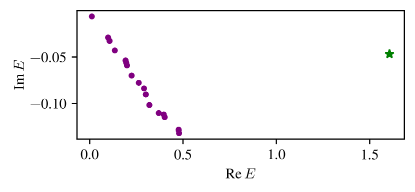
Figure 1: Complex-$E$ spectrum at $L=20$ for the two-body potential given by Eq. (54) showing 40 eigenvalues with the largest imaginary parts. The resonance of interest is highlighted with a star symbol.

Being able to identify the resonance state of interest, we can repeat the calculation for a range of volumes and perform the fits as described at the beginning of this section. The result is shown in Fig. 2. For comparison, we fit both the leading-order (LO) form of the volume dependence, Eq. (30), as well as the “NLO” form given in Eq. (43). From the LO fit we obtain $E_{\infty}=1.605676(13)-0.046603(13)\mathrm{i}$, while the NLO fit gives $E_{\infty}=1.6056798(27)-0.0465947(27)\mathrm{i}$. in good agreement with the known value. The uncertainties quoted here for our calculation are the standard errors reported by the fitting routine.

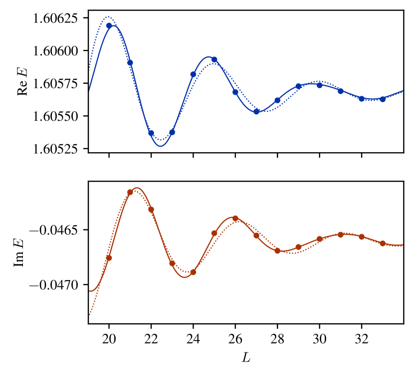
Figure 2: Finite-volume spectrum for the $S$-wave resonance for the potential given by Eq. (54). The real (imaginary) part of the energy is shown in the upper (lower) panel. For each, we show the result of fitting the volume dependence at LO (dotted line) and NLO (solid line).

IV.2 P-wave resonance

To study a P-wave example, we use the potential

$$V(r)={-}10\exp({-}r^{2})\,,$$ (55)

which we find to support a resonance at $E_{\infty}=0.25822632-0.16432586\mathrm{i}$ from a momentum space calculation with complex-scaling (see Ref. [62] for details) with the momentum cutoff and the mesh resolution increased until the value converged to the quoted precision. The volume dependence for this state, calculated with with a DVR basis size of $N=96$ and a complex-scaling angle of $\phi=\pi/6$, is shown Fig. 3. From fitting The LO fit for this resonance yields $E_{\infty}=0.25817(7)-0.16431(7)\mathrm{i}$, while at NLO we obtain $E_{\infty}=0.258257(31)-0.164315(31)\mathrm{i}$. Both results agree well with the reference value. We see a marginal improvement in this case at NLO, which is more noticeable in Fig. 3: clearly the fit residuals are reduced when using the NLO volume dependence (solid line in the figure).

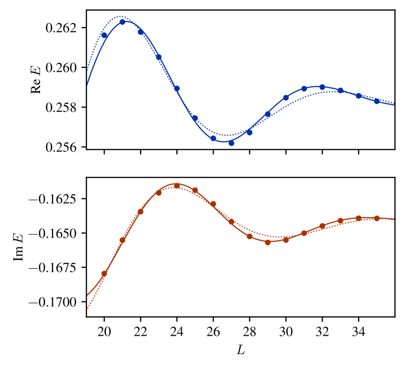
Figure 3: Finite-volume spectrum for the $P$-wave resonance for the potential given by Eq. 55. The real (imaginary) part of the energy is shown in the upper (lower) panel. For each, we show the result of fitting the volume dependence at LO (dotted line) and NLO (solid line).

IV.3 S-wave bound state

As mentioned in Sec. II.2, the volume dependence derived in this work is valid not only for resonances, but also for bound states calculated with complex scaling. Moreover, instead of varying the volume, it is also possible to keep $L$ fixed and then fit the relevant equations as a function of the complex-scaling rotation angle $\phi$. As an example for this approach, we look at the $S$-wave bound state with $E_{\infty}={-}2.5434016$ generated by the same potential (55) we used to generate a P-wave resonance. For this, we use an FV-DVR calculation with a box size of $L=6$ and a DVR basis size of $N=30$. The rotation angle is varied in a range as shown in Fig. 4, and curve fitting is performed as described previously, except that now the independent variable is $\phi$ instead of $L$. From the LO fit we obtain $E_{\infty}={-}2.54347(6)-0.00002(6)\mathrm{i}$ and the NLO yields $E_{\infty}={-}2.54344(6)-0.00004(6)\mathrm{i}$. The real parts are in excellent agreement with the reference value, with marginal improvement at NLO. The imaginary parts (which should be regarded as numerical artifacts), are negligibly small. We emphasize that in principle the same approach can be used to extract resonance properties at fixed volume, except that the available range of angles is restricted by the condition that $\phi>{-}\arg E/2$.

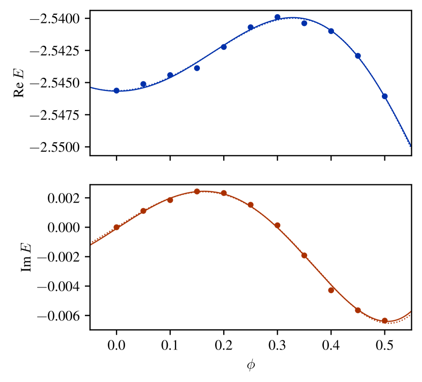
Figure 4: Finite-volume energy, as a function of the complex-scaling angle $\phi$, for the $S$-wave bound state generated by the potential given by Eq. 55. The real (imaginary) part of the energy is shown in the upper (lower) panel. For each, we show the result of fitting the volume dependence at LO (dotted line) and NLO (solid line).

IV.4 Three-boson resonance

Finally, to show that FV-DVR prescription with complex scaling works just as well beyond the two-body sector, we calculate the finite-volume three-body spectrum for a system of bosons where the pairwise interaction between particles is given by the potential 54. Using the method of avoided crossings, Ref.[34] estimates reports for this scenario a resonance at $\mathrm{Re}(E)=4.18(8)$, with an unknown width. We study this system with a complex-scaling angle $\phi=\pi/9$, employing symmetrization to restrict the calculation to bosonic states with positive parity. We find indeed a resonance close to the expected position, identified in the same manner as discussed for two-body resonances. The volume dependence of this state is shown in Fig. 5, where in order to study numerical convergence with the DVR basis size, we compare results for $N=22$ and $N=24$. From this comparison we conclude that the real part of the energy is well converged up to at least $L=16$, whereas the imaginary part shows somewhat larger remaining artifacts due to a lack of (ultraviolet) convergence.

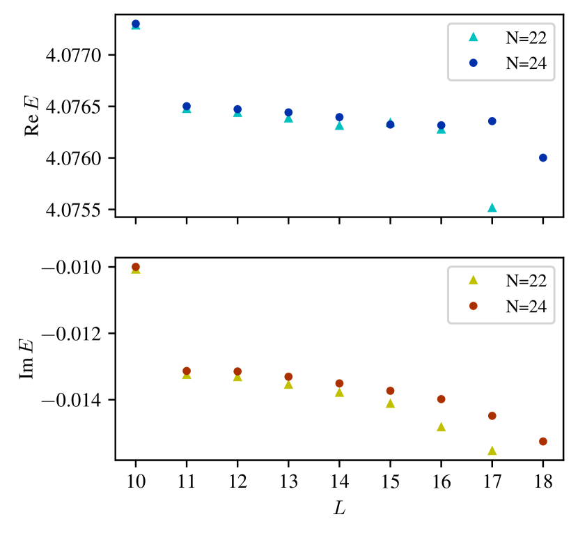
Figure 5: Finite-volume spectrum for the three-boson resonance generated by the potential in Eq. 54. The real (imaginary) part of the energy is shown in the upper (lower) panel. Since the volume dependence of this state is unknown, this figure does not include any fitted curves.

Since we do not know the functional form for the volume dependence of this three-body state, we cannot use the fitting technique to directly infer the infinite-volume energy for this resonances. However, one should expect that similar to two-body resonances the norm of the energy to converges exponentially with increasing $L$, as pointed out previously in Ref. [41]. Indeed, noting the inflated vertical axis scale in Fig. 5, we point out that compared to the overall magnitude, both the real and the imaginary part of the energy show only relatively small variations over the range $L=11\cdot 16$ shown in the figure. As a very rough estimate for the infinite-volume properties, we merely take the average of the $N=24$ results over this range to obtain $E_{\infty}\approx 4.07641(8)-0.01347(34)\mathrm{i}$. The real part we find is close to the value $\mathrm{Re}(E)=4.18(8)$ reported in Ref. [34], although the respective uncertainties do not quite overlap. Since we see very little variation of $\mathrm{Re}(E)$ with $L$ or $N$, we presume that Ref. [34] likely underestimated the uncertainty stemming from the method of avoided level crossings.

V Summary and outlook

In this work, we have studied complex scaling in finite periodic boxes as a framework for studying few-body quantum systems, in particular systems that host resonances. We derived explicitly the volume dependence of two-body resonances and bound states (i.e., energy levels that correspond to isolated S-matrix poles in infinite volume), including the first corrections to the leading behavior. We furthermore developed a a concrete numerical implementation of the technique and used this to test the expressions we derived for the volume dependence with several explicit examples.

Our approach combines two established approaches. While few-body resonances have been studied in finite-volume without complex scaling by looking for avoided crossings in the finite-volume spectrum [34, 29], that approach can quickly become numerically expensive, and it does not readily provide access to resonance widths in general. Although finite-volume eigenvector continuation [35] has been shown to significantly reduce the numerical cost of such studies, the approach we presented here has the appeal that via complex scaling resonances can be found in much smaller boxes, and the analytical expressions we derived then make it possible to directly infer infinite-volume resonance properties, including the decay width. Ref. [41] employs an analytic continuation to imaginary box sizes in order to study resonances in finite-volume, also including widths, but that method is still indirect in the sense that it extracts resonance properties from peaks in transition amplitudes instead of directly identifying complex energy eigenstates of the finite-volume Hamiltonian, as we do in this work.

While we have rigorously derived the volume dependence here only for two-body systems, we expect our results to directly generalize to few-body states if the dominant decay (or breakup, in the case of bound states) mode is into two clusters, following the derivation for bound states without complex scaling [4]. For systems where this is not the case, such as the three-boson example that we considered in this work, it is still possible to obtain good approximations to the infinite-volume resonance properties by calculating in relatively large boxes.

Our findings have applications in various areas of physics, ranging from cold atoms to nuclear physics. In particular, it would be interesting to study Efimov trimers (and associated tetramers) [63, 64] in finite volume with complex scaling, and we also plan to investigate few-neutron systems using complex scaling in finite volume. Naturally, our results enable finite-volume studies of resonances in a a variety atomic nuclei, and developing an extension to systems of charged particles, as recently done for bound states [65], will further broaden the range of systems that our method can be applied to. Finally, it will be interesting to explore the resonance eigenvector continuation method developed in Ref. [35] to study extrapolations from bound states to resonances in finite volume.