Terahertz-Band Direction Finding With Beam-Split and Mutual Coupling Calibration

Abstract

Terahertz (THz) band is currently envisioned as the key building block to achieving the future sixth generation (6G) wireless systems. The ultra-wide bandwidth and very narrow beamwidth of THz systems offer the next order of magnitude in user densities and multi-functional behavior. However, wide bandwidth results in a frequency-dependent beampattern causing the beams generated at different subcarriers split and point to different directions. Furthermore, mutual coupling degrades the system’s performance. This paper studies the compensation of both beam-split and mutual coupling for direction-of-arrival (DoA) estimation by modeling the beam-split and mutual coupling as an array imperfection. We propose a subspace-based approach using multiple signal classification with CalibRated for bEAam-split and Mutual coupling (CREAM-MUSIC) algorithm for this purpose. Via numerical simulations, we show the proposed CREAM-MUSIC approach accurately estimates the DoAs in the presence of beam-split and mutual coupling.

I Introduction

Terahertz (THz) band ($0.1$-$10$ THz) is widely viewed as a technology to enable significant performance enhancements in sixth-generation (6G) wireless networks [1]. An accuracy of milli-degree in direction-of-arrival (DoA) estimation is critical to guaranteeing the reliability of THz sensing as well as communications [2, 3]. However, significant challenges remain in realizing this goal at the THz band owing to high path losses, complex propagation/scattering phenomena, and the use of extremely large arrays [4, 1, 5].

In particular, the ultra-dense integration of the antennas in the THz array is accompanied by mutual coupling (MC) which leads to degradation in the direction finding accuracy [2, 6, 7]. The existing works on reducing MC in THz mostly involve array design with new metamaterials [8], graphene monolayers [9], THz metasurfaces [10] or frequency-selective graphene surfaces [7], while MC calibration at THz-band via signal processing remains relatively unexamined. Furthermore, THz arrays also suffer from beam-split arising from the subcarrier-independent (SI) analog beamformers (ABs) [11, 12, 13]. This causes the generated beams at different subcarriers split and point to different directions. At lower frequencies (e.g., up to millimeter-wave [14]), beam-squint is used to describe the same phenomenon, and negative group-delay networks are used to compensate for it [15]. Whereas beam-squint causes slight deviations in the beam direction while they still cover the targets with their mainlobes, the generated beams are completely non-overlapping in beam-split. The latter is, therefore, a more severe form of the former (Fig. 1a). This angular deviation eventually impacts MC, which is direction-dependent because of the directional beampattern [16]. The existing techniques to mitigate beam-split are mostly hardware-based [11]. Specifically, additional hardware components such as time-delayer networks to realize subcarrier-dependent (SD) ABs, they are expensive because each phase shifter is connected to multiple delayer elements. Further, each such element consumes approximately $100$ mW which is more than that of a single phase shifter ($40$ mW) at THz [3].

Although THz channel estimation [12] and hybrid analog/digital beamforming [11, 17] under beam-split have been explored in prior THz studies, these algorithms did not examine either DoA estimation or MC calibration. The hybrid architectures at mm-Wave [18, 19] and THz [2] so far employ orthogonal matching pursuit (OMP) [18], maximum likelihood (ML) [19] and MUltiple SIgnal Classification (MUSIC) [2, 6] for DoA estimation but exclude beam-split and MC. The calibration of beam-split in THz systems is considered for different array geometries, e.g., uniform linear/rectangular array (ULA/URA) [20, 12, 21]. Specifically, the ULA provides a simple design whereas the URA-based THz systems allow a compact and efficient design with array/group of subarrays architecture [17]. While the calibration procedure is the similar, the use of URA introduces the calibration of beam-split in both azimuth and elevation.

In this work, contrary to previous works, we address the aforementioned shortcomings by considering beam-split as an array imperfection in a similar way as MC has been investigated in the well-studied array calibration theory [22, 16, 23]. Specifically, we model the beam-split errors as a diagonal matrix, which represents a linear transformation between the nominal and actual steering vectors corrupted by beam-split. Using this transformation and incorporating the signal-noise subspace orthogonality, we develop a calibrated for beaam-split and MC MUSIC (CREAM-MUSIC) algorithm to obtain accurate DoA estimates. In particular, we introduce an alternating approach, wherein the DoAs, beam-split, and MC coefficients are iteratively estimated. For DoA, while the degree of beam-split is proportionally known a priori, it depends on the unknown target direction. For example, consider $f_{m}$ and $f_{M}$ to be the frequencies for, respectively, the $m$-th and last/highest subcarriers. When $\theta$ is the physical target direction, then the spatial direction corresponding to the $m$-th-subcarrier is shifted by $\frac{f_{m}}{f_{M}}\theta$. We then construct the CREAM-MUSIC spectra which accounts for this deviation and thereby ipso facto mitigates the effect of beam-split (Fig. 1b-c).

Figure 1: The MUSIC spectra of (a) all subcarriers without beam-split compensation, (b) all subcarriers with beam-split compensation, (c) CREAM-MUSIC algorithm for the source location depicted with vertical line. $f_{c}=300$ GHz, $B=30$ GHz, $M=11$, $\tilde{\theta}=60^{\circ}$, $N=128$ and $N_{\mathrm{RF}}=8$.

II System Model & Problem Formulation

Consider a wideband THz ultra-massive multiple-input multiple-output uplink scenario, wherein the base-station (BS) employs hybrid analog/digital beamformers with $N$-element ULA and $N_{\mathrm{RF}}$ radio-frequency (RF) chains. In sensing applications, the equivalent signals would be from $K$ targets. Without loss of generality, assume the targets are in the far-field of the BS with the physical DoAs $\theta_{k}$ for $k\in\{1,\cdots,K\}=\mathcal{K}$, where $\theta_{k}=\sin\tilde{\theta}_{k}$ ($\tilde{\theta}_{k}\in[-\frac{\pi}{2},\frac{\pi}{2}]$).

To begin with, we first consider the conventional MC- and beam-split- free scenario, wherein the $N\times 1$ steering vector corresponding to the $k$-th target is

$${\mathbf{a}}(\theta_{k})=[1,e^{\mathrm{j}2\pi\frac{d}{\lambda^{\star}}\theta_{k}},\cdots,e^{\mathrm{j}2\pi(N-1)\frac{d}{\lambda^{\star}}\theta_{k}}]^{\textsf{T}},$$ (1)

where $d$ stands for antenna spacing and $\lambda^{\star}=\frac{\nu}{f_{M}}$ denotes the wavelength corresponding to the highest subcarrier frequency. Hence, $d$ is selected as $d=\frac{\nu}{2\max_{m}f_{m}}=\frac{\nu}{2f_{M}}$ in order to avoid spatial aliasing [24]. Here, $\nu$ is speed of light and $f_{m}=f_{c}+\frac{B}{M}(m-1-\frac{M-1}{2})$ is the $m$-th subcarrier frequency ($m\in\{1,\cdots,M\}=\mathcal{M}$) with $f_{c}$ and $B$ being the carrier frequency and total bandwidth, respectively.

In order to sense the targets, the BS employs the sensing signal $\mathbf{s}_{m}(t_{i})\in\mathbb{C}^{N_{\mathrm{RF}}}$ and the SI precoder $\mathbf{F}\in\mathbb{C}^{N\times N_{\mathrm{RF}}}$. Then, the BS activates $N_{\mathrm{RF}}$ RF chains and applies $\mathbf{F}\in\mathbb{C}^{N\times N_{\mathrm{RF}}}$ to the sensing signal $\mathbf{s}_{m}(t_{i})$, and the $N\times 1$ transmit signal becomes $\mathbf{x}_{m}(t_{i})=\mathbf{F}\mathbf{s}_{m}(t_{i})$ where $i=1,\cdots,T$ and $T$ is the number of data snapshots.

Beam-Split: During the search phase of the THz radar, the AB is designed with the structure of steering vectors corresponding to the search directions. For an arbitrary $\mathbf{a}(\theta_{k})$ for direction $\theta_{k}$. Then, the $n$-th element of $\mathbf{a}(\theta_{k})$ is defined as $[\mathbf{a}(\theta_{k})]_{n}=1/\sqrt{N}\exp\big{\{}\mathrm{j}(n-1)\frac{2\pi d}{\lambda_{m}}\theta_{k}\big{\}}$, i.e.,

$$[\mathbf{a}(\theta_{k})]_{n}=1/\sqrt{N}\exp\big{\{}\mathrm{j}(n-1)\pi\eta_{m}\theta_{k}\big{\}},$$ (2)

where $\eta_{m}=\frac{f_{m}}{f_{M}}$. We can see that the direction of AB designed for $\theta_{k}$ is split and points to the spatial direction $\bar{\theta}_{k,m}=\eta_{m}\theta_{k}$. It is also clear that when $f_{m}=f_{M}$, we have $\bar{\theta}_{k,m}=\theta_{k}$, which leads to the definition in (1).

Lemma 1.

Let $\mathbf{a}(\bar{\theta}_{m})$ and $\mathbf{a}(\theta)$ be the beam-split-corrupted and nominal steering vectors for an arbitrary direction $\theta$ and subcarrier $m\in\mathcal{M}$ as defined in (2) and (1), respectively. Then, $\mathbf{a}(\bar{\theta}_{m})$ achieves the maximum array gain, i.e., $A_{G}(\theta,m)=\frac{|\mathbf{a}^{\textsf{H}}(\theta)\mathbf{a}(\bar{\theta}_{m})|^{2}}{N^{2}}$, if $\bar{\theta}_{m}=\eta_{m}\theta$.

Proof.

The array gain varies across the whole bandwidth as $A_{G}({\theta},{m})=\frac{|\mathbf{a}^{\textsf{H}}(\theta)\mathbf{a}(\bar{\theta}_{m})|^{2}}{N^{2}}.$ By using (1) and (2), $A_{G}({\theta},{m})$ is

$$A_{G}({\theta},{m})=\frac{1}{N^{2}}\left|\sum_{n_{1}=1}^{N}\sum_{n_{2}=1}^{N}e^{-\mathrm{j}\pi\left((n_{1}-1){\bar{\theta}_{m}}-(n_{2}-1)\frac{\lambda_{M}\theta}{\lambda_{m}}\right)}\right|^{2}$$

$$=\left|\sum_{n=0}^{N-1}\frac{e^{-\mathrm{j}2\pi nd\left(\frac{\bar{\theta}_{m}}{\lambda_{M}}-\frac{\theta}{\lambda_{m}}\right)}}{N}\right|^{2}=\left|\sum_{n=0}^{N_{\mathrm{T}}-1}\frac{e^{-\mathrm{j}2\pi nd\frac{(f_{c}\Phi_{m}-f_{m}\Phi)}{c_{0}}}}{N}\right|^{2}$$

$$=\left|\frac{1-e^{-\mathrm{j}2\pi Nd\frac{(f_{M}\bar{\theta}_{m}-f_{m}\theta)}{\nu}}}{N(1-e^{-\mathrm{j}2\pi d\frac{(f_{M}\bar{\theta}_{m}-f_{m}\theta)}{\nu})}}\right|^{2}=\left|\frac{\sin(\pi N\mu_{m})}{N\sin(\pi\gamma_{m})}\right|^{2}=|\xi(\mu_{m})|^{2},$$

where $\mu_{m}=d\frac{(f_{M}\bar{\theta}_{m}-f_{m}\theta)}{\nu}$. The array gain implies that most of the power is focused only on a small portion of the beamspace due to the power-focusing capability of $\xi(\cdot)$, which substantially reduces across the subcarriers as $|f_{m}-f_{M}|$ increases. Furthermore, $|\xi(\mu_{m})|^{2}$ gives peak when $\mu_{m}=0$, i.e., $f_{M}\bar{\theta}_{m}-f_{m}\theta=0$, which yields $\bar{\theta}_{m}=\eta_{m}\theta$. ∎

Above lemma indicates that the split direction $\bar{\theta}_{m}$ should be taken into account to achieve accurate DoA estimation performance. Finally, we define the relationship between the nominal and beam-split-corrupted steering vectors as

$$\mathbf{a}(\bar{\theta}_{m,k})=\mathbf{B}_{m,k}\mathbf{a}(\theta_{k}),$$ (3)

where $\mathbf{B}_{m,k}=\mathrm{diag}\{b_{m,k,1},\cdots,b_{m,k,N}\}$ is an $N\times N$ diagonal matrix with $b_{m,k,n}=\exp\{\mathrm{j}(n-1)\pi\Delta_{m,k}\}$, where $\Delta_{m,k}$ is defined as beam-split, i.e., $\Delta_{m,k}=\bar{\theta}_{m,k}-\theta_{k}.$

Mutual Coupling: Experimentally, the MC matrix is found from the inverse of the measurement transformation matrix $\mathbf{Z}_{m}\in\mathbb{C}^{N\times N}$, which maps the coupled voltages to the uncoupled voltages [25, 26, 27] as $\mathbf{Z}_{m}\mathbf{V}_{m}=\mathbf{U}_{m}$. Here, $\mathbf{V}_{m}=\left[\mathbf{v}_{m}^{1},\cdots,\mathbf{v}_{m}^{\Omega}\right]\in\mathbb{C}^{N\times\Omega}$ comprises the coupled measurements collected for $\Omega\geq N$ distinct directions when all the antennas are residing in the array whereas $\mathbf{U}_{m}=\left[\mathbf{u}_{m}^{1},\cdots,\mathbf{u}_{m}^{\Omega}\right]\in\mathbb{C}^{N\times\Omega}$ is obtained with $N$ antenna elements, each of which is considered one-by-one separately while the remaining $N-1$ antennas are removed. Then, the direction-independent MC matrix is obtained as $\mathbf{C}_{m}=\mathbf{Z}_{m}^{-1}$. When the MC is DD, it should be computed for a certain angular sectors [16].

The MC matrix of a ULA is represented by an $L$-banded Toeplitz matrix [22, 28, 29]. Define $\mathbf{C}_{m}(\theta_{k})\in\mathbb{C}^{N\times N}$ as the SD and direction-dependent MC matrix with $L$ MC coefficients, i.e., $\mathbf{C}_{m}(\theta_{k})=\mathrm{Toeplitz}\{1,c_{m,k,1},\cdots,c_{m,k,L},0,\cdots,0\}$, where $\{c_{m,k,l}\}_{l=1}^{L}$ are the distinct MC coefficients. Denote the actual steering vector by $\tilde{\mathbf{a}}(\bar{\theta}_{m,k})\in\mathbb{C}^{N}$. The steering vector corrupted by both beam-split and MC becomes

$${\color[rgb]{0,0,0}\tilde{\mathbf{a}}(\bar{\theta}_{m,k})=\mathbf{C}_{m}(\theta_{k})\mathbf{a}(\bar{\theta}_{m,k})=\mathbf{C}_{m}(\theta_{k})\mathbf{B}_{m,k}\mathbf{a}(\theta_{k}),}$$ (4)

for which we define the MC-corrupted steering matrix in a compact for as $\mathbf{D}_{m}=[\tilde{\mathbf{a}}(\bar{\theta}_{m,1}),\cdots,\tilde{\mathbf{a}}(\bar{\theta}_{m,K})]\in\mathbb{C}^{N\times K}$.

Our goal is to estimate the DoAs of the targets $\{\theta_{k}\}_{k=1}^{K}$ while accurately compensating for beam-split and MC.

III Proposed Method

Define ${\mathbf{X}}_{m}=[\mathbf{x}_{m}(t_{1}),\cdots,\mathbf{x}_{m}(t_{T})]\in\mathbb{C}^{N\times T}$ as the radar probing signal transmitted by the BS for $T$ data snapshots along the fast-time axis [30], where $\mathbb{E}\{{\mathbf{X}}_{m}{\mathbf{X}}_{m}^{\textsf{H}}\}=\frac{P_{\mathrm{r}}T}{MN}\mathbf{I}_{N}$, for which $\mathbf{F}\mathbf{F}^{\textsf{H}}=1/N$, and $P_{\mathrm{r}}$ is the radar transmit power. Limited number of RF chains yield $N_{\mathrm{RF}}\times 1$ received baseband data vector. When $K\geq N_{\mathrm{RF}}$, it results in poorer parameter estimation [24, 31]. To collect the full array data from $N_{\mathrm{RF}}$ RF chains, we follow a subarrayed approach. That is, the BS activates the antennas in a subarrayed manner to apply the $N\times N_{\mathrm{RF}}$ analog beamforming matrix $\widetilde{\mathbf{W}}=\left[\overline{\mathbf{W}}_{1}^{\textsf{T}},\cdots,\overline{\mathbf{W}}_{J}^{\textsf{T}}\right]^{\textsf{T}}$. Then, the BS collects the received target echoes for $J=\frac{N}{N_{\mathrm{RF}}}$ time slots. The target DoAs remain invariant within a time slot but change across different time slots. This is reasonable for the THz system, wherein the symbol time is of the order of picoseconds [2, 30]. Then, for the $j$-th time slot, the BS applies the combiner matrix $\mathbf{W}_{j}=\left[\begin{array}[]{c}\mathbf{0}_{jN_{\mathrm{RF}}\times N_{\mathrm{RF}}}\\ \overline{\mathbf{W}}_{j}\\ \mathbf{0}_{N-(j+1)N_{\mathrm{RF}}\times N_{\mathrm{RF}}}\end{array}\right]\in\mathbb{C}^{N\times N_{\mathrm{RF}}}$, where $\overline{\mathbf{W}}_{j}\in\mathbb{C}^{N_{\mathrm{RF}}\times N_{\mathrm{RF}}}$ represents the $j$-th block of $\widetilde{\mathbf{W}}$ corresponding to the $j$-th subarray. Then, the $N_{\mathrm{RF}}\times T$ echo signal from the $K$ targets at the $j$-th time slot is

$${\mathbf{Y}}_{m,j}=\sum_{k=1}^{K}\beta_{k}\mathbf{W}_{j}^{\textsf{H}}\tilde{\mathbf{a}}(\bar{\theta}_{m,k})\left[\tilde{\mathbf{a}}(\bar{\theta}_{m,k})\right]^{\textsf{T}}{\mathbf{X}}_{m}+\tilde{\mathbf{N}}_{m,j},$$ (5)

where $\beta_{k}\in\mathbb{C}$ denotes the reflection coefficient of the $k$-th target. $\tilde{\mathbf{N}}_{m,j}=\mathbf{W}_{j}^{\textsf{H}}\bar{\mathbf{N}}_{m,j}\in\mathbb{C}^{N_{\mathrm{RF}}\times T}$ is representing the noise term, where $\bar{\mathbf{N}}_{m,j}=[\bar{\mathbf{n}}_{m,j}(t_{1}),\cdots,\bar{\mathbf{n}}_{m,j}(t_{T})]\in\mathbb{C}^{N\times T}$ with $\bar{\mathbf{n}}_{m,j}(t_{i})\sim\mathcal{CN}(\mathbf{0},{\sigma}_{n}^{2}\mathbf{I}_{N})$. Denote the target steering matrix and reflection coefficients by ${\mathbf{A}}_{m,j}=\mathbf{W}_{j}^{\textsf{H}}\mathbf{D}_{m}\in\mathbb{C}^{N_{\mathrm{RF}}\times K}$ and $\boldsymbol{\Pi}=\mathrm{diag}\{\beta_{1},\cdots,\beta_{K}\}\in\mathbb{C}^{K\times K}$, then (5) becomes ${\mathbf{Y}}_{m,j}={\mathbf{A}}_{m,j}\boldsymbol{\Pi}{\mathbf{D}}_{m}^{\textsf{T}}{\mathbf{X}}_{m}+\tilde{\mathbf{N}}_{m,j}.$ Stacking all $\mathbf{Y}_{m,j}$ into a single $N\times T$ matrix leads to the overall observation matrix $\mathbf{Y}_{m}\in\mathbb{C}^{N\times T}$ as

$$\mathbf{Y}_{m} =\left[\mathbf{Y}_{m,1}^{\textsf{T}},\cdots,\mathbf{Y}_{m,J}^{\textsf{T}}\right]^{\textsf{T}}=\mathbf{A}_{m}\boldsymbol{\Pi}\mathbf{D}_{m}^{\textsf{T}}\mathbf{X}_{m}+\tilde{\mathbf{N}}_{m},$$ (6)

where $\mathbf{A}_{m}=\left[\mathbf{A}_{m,1}^{\textsf{T}},\cdots,\mathbf{A}_{m,J}^{\textsf{T}}\right]^{\textsf{T}}=\mathbf{W}^{\textsf{H}}\mathbf{D}_{m}\in\mathbb{C}^{N\times K}$, $\mathbf{W}=\left[{\mathbf{W}}_{1},\cdots,{\mathbf{W}}_{J}\right]\in\mathbb{C}^{N\times N}$, and $\tilde{\mathbf{N}}_{m}=\left[\tilde{\mathbf{N}}_{m,1}^{\textsf{T}},\cdots,\tilde{\mathbf{N}}_{m,J}^{\textsf{T}}\right]^{\textsf{T}}$. We now introduce an alternating algorithm, wherein the beam-split-corrected DoA angles and the MC coefficients are estimated iteratively such that MC parameters are kept fixed while estimating the DoA angle or vice versa.

III-A DoA and Beam-Split Estimation

In order to estimate the target directions, we invoke the wideband MUSIC algorithm [31, 24]. Define $\mathbf{R}_{m}\in\mathbb{C}^{N\times N}$ as the covariance matrix of ${\mathbf{Y}}_{m}$, i.e.,

$$\mathbf{R}_{m} =\frac{1}{T}{\mathbf{Y}}_{m}{\mathbf{Y}}_{m}^{\textsf{H}}=\frac{1}{T}{\mathbf{A}}_{m}\left(\frac{P_{\mathrm{r}}T}{MN}\widetilde{\boldsymbol{\Pi}}\right){\mathbf{A}}_{m}^{\textsf{H}}+\frac{1}{T}\tilde{\mathbf{N}}_{m}\tilde{\mathbf{N}}_{m}^{\textsf{H}}$$

$$\approxeq\frac{P_{\mathrm{r}}}{MN}{\mathbf{A}}_{m}\widetilde{\boldsymbol{\Pi}}{\mathbf{A}}_{m}^{\textsf{H}}+{\sigma}_{n}^{2}\mathbf{I}_{{N}},$$ (7)

where $\tilde{\mathbf{N}}_{m}\tilde{\mathbf{N}}_{m}^{\textsf{H}}\approxeq{\sigma}_{n}^{2}T/N\mathbf{I}_{N}$ and $\widetilde{\boldsymbol{\Pi}}\in\mathbb{C}^{K\times K}$ is defined as $\widetilde{\boldsymbol{\Pi}}=\boldsymbol{\Pi}\mathbf{D}^{\textsf{T}}\mathbf{D}^{*}\boldsymbol{\Pi}^{*}$. Then, the eigendecomposition of $\mathbf{R}_{m}$ yields $\mathbf{R}_{m}=\mathbf{U}_{m}\boldsymbol{\Theta}_{m}\mathbf{U}_{m}^{\textsf{H}},$ where $\boldsymbol{\Theta}_{m}\in\mathbb{C}^{N\times N}$ is a diagonal matrix composed of the eigenvalues of $\mathbf{R}_{m}$ in a descending order, and $\mathbf{U}_{m}=\left[\mathbf{U}_{m}^{\mathrm{S}}\hskip 2.0pt\mathbf{U}_{m}^{\mathrm{N}}\right]\in\mathbb{C}^{N\times N}$ corresponds to the eigenvector matrix; $\mathbf{U}_{m}^{\mathrm{S}}\in\mathbb{C}^{N\times K}$ and $\mathbf{U}_{m}^{\mathrm{N}}\in\mathbb{C}^{N\times N-K}$ are the signal and noise subspace eigenvector matrices, respectively. The columns of $\mathbf{U}_{m}^{\mathrm{S}}$ and ${\mathbf{A}}_{m}$ span the same space that is orthogonal to the eigenvectors in $\mathbf{U}_{m}^{\mathrm{N}}$ as $\|{\mathbf{U}_{m}^{\mathrm{N}}}^{\textsf{H}}(\mathbf{W}^{\textsf{H}}\tilde{\mathbf{a}}(\bar{\theta}_{m,k}))\|_{2}^{2}$, i.e., $\|{\mathbf{U}_{m}^{\mathrm{N}}}^{\textsf{H}}(\mathbf{W}^{\textsf{H}}\mathbf{C}_{m}(\theta_{k})\mathbf{B}_{m,k}\mathbf{a}(\theta_{k}))\|_{2}^{2}=0,$ for $k\in\mathcal{K}$ and $m\in\mathcal{M}$ [31]. Thus, given the MC matrix $\mathbf{C}_{m}(\theta)$, the conventional MUSIC spectra is given by

$$P(\theta)=\sum_{m=1}^{M}P_{m}(\theta),$$ (8)

where $P_{m}(\theta)$ is the spectrum corresponding to the $m$-th subcarrier as $P_{m}(\theta)=\frac{1}{f(m,k)}$, where $f(m,k)=\mathbf{a}^{\textsf{H}}(\theta)\mathbf{C}_{m}^{\textsf{H}}(\theta)\mathbf{W}\mathbf{U}_{m}^{\mathrm{N}}{\mathbf{U}_{m}^{\mathrm{N}}}^{\textsf{H}}\mathbf{W}^{\textsf{H}}\mathbf{C}_{m}(\theta)\mathbf{a}(\theta).$ The MUSIC spectra in (8) yields $MK$ peaks, which are deviated due to beam-split (see Fig. 1a) while correct MUSIC spectra should include $K$ peaks which are aligned for $m\in\mathcal{M}$. In other words, beam-split-corrected steering vectors should be used to accurately compute the MUSIC spectra. The CREAM-MUSIC accounts for this deviation by employing beam-split-aware steering vectors $\mathbf{e}_{m}(\theta)=\mathbf{W}^{\textsf{H}}\mathbf{C}_{m}(\theta)\mathbf{a}(\bar{\theta}_{m})\in\mathbb{C}^{N}$. Then, the CREAM-MUSIC spectra is $\widetilde{P}(\theta)=\sum_{m=1}^{M}\widetilde{P}_{m}(\theta),$ where

$$\widetilde{P}_{m}(\theta)=\frac{1}{\mathbf{e}_{m}^{\textsf{H}}(\theta)\mathbf{U}_{m}^{\mathrm{N}}{\mathbf{U}_{m}^{\mathrm{N}}}^{\textsf{H}}\mathbf{e}_{m}(\theta)},$$ (9)

for which, the $K$ highest peaks of (9) correspond to the estimated target DoAs $\{\hat{\theta}_{k}\}_{k=1}^{K}$, and the beam-split is computed as $\hat{\Delta}_{m,k}=(\eta_{m}-1)\hat{\theta}_{k}$, for $m\in\mathcal{M}$, $k\in\mathcal{K}$. Note that combining the spectra of $M$ subcarriers results in only a single peak-search in place of separately estimating the DoAs for each subcarrier.

III-B Mutual Coupling Estimation

Define $\mathbf{c}_{m,k}=[c_{m,k,1},\cdots,c_{m,k,L}]^{\textsf{T}}$ as the $L\times 1$ vector MC coefficients. Then, we construct the following useful matrix-vector transformation between $\mathbf{c}_{m,k}$ and $\mathbf{C}_{m}(\theta_{k})$, i.e., $\mathbf{C}_{m}(\theta_{k})=\mathbf{T}_{m,k}\mathbf{c}_{m,k},$ where $\mathbf{T}_{m,k}=\left[\mathbf{S}_{m,1}\mathbf{a}(\bar{\theta}_{m,k}),\cdots,\mathbf{S}_{m,L}\mathbf{a}(\bar{\theta}_{m,k})\right]\in\mathbb{C}^{N\times L}$, for which $\mathbf{S}_{m,l}$ is an ${N\times N}$ matrix, and it is defined for any array geometry as $\mathbf{S}_{m,l}=\left\{\begin{array}[]{ll}1,&\text{if }[\mathbf{C}_{m}(\theta_{k})]_{i,j}=c_{m,k,l}\\ 0,&\text{otherwise}\end{array}\right.$ [16]. Given the DoAs $\{\theta_{k}\}_{k=1}^{K}$, we solve the following optimization problem to estimate $\mathbf{c}_{m,k}$, i.e., $\operatorname*{minimize}_{\mathbf{c}_{m,k}}\hskip 3.0pt\sum_{m=1}^{M}f(m,k),\hskip 5.0pt\operatorname*{s.\hskip 3.0ptt.:\hskip 3.0pt}c_{m,k,1}=1,$ which is equivalent to $\operatorname*{minimize}_{\mathbf{c}_{m,k}}\hskip 3.0pt\sum_{m=1}^{M}\mathbf{c}_{m,k}^{\textsf{H}}\boldsymbol{\Sigma}_{m,k}\mathbf{c}_{m,k},\hskip 3.0pt\operatorname*{s.\hskip 3.0ptt.:\hskip 3.0pt}\mathbf{v}^{\textsf{T}}\mathbf{c}_{m,k}=1,$ where $\mathbf{v}=[1,0,\cdots,0]^{\textsf{T}}\in\mathbb{C}^{L\times 1}$ and $\boldsymbol{\Sigma}_{m,k}\in\mathbb{C}^{L\times L}$ is $\boldsymbol{\Sigma}_{m,k}=\mathbf{T}_{m,k}^{\textsf{H}}\mathbf{W}\mathbf{U}_{m}^{\mathrm{N}}{\mathbf{U}_{m}^{\mathrm{N}}}^{\textsf{H}}\mathbf{W}^{\textsf{H}}\mathbf{T}_{m,k}.$ Then, the closed-form solution for $\mathbf{c}_{m,k}$ is

$$\hat{\mathbf{c}}_{m,k}=\boldsymbol{\Sigma}_{m,k}^{-1}\mathbf{v}\left(\mathbf{v}^{\textsf{T}}\boldsymbol{\Sigma}_{m,k}^{-1}\mathbf{v}\right)^{-1}.$$ (10)

In Algorithm 1, we present the proposed alternating approach to effectively estimate the DoAs, beam-split, and MC coefficients. Specifically, we first partition the angular search space into $S$ sectors as $\Phi=\cup_{s=1}^{S}\Psi_{s}$, where $\Phi=[-\frac{\pi}{2},\frac{\pi}{2}]$ for a ULA, and $\Psi_{s}$ denotes the angular sector, for which the direction-dependent MC matrix $\mathbf{C}_{m}(\Psi_{s})$ is kept fixed [16]. Then, the estimates of the DoAs and MC coefficients are alternatingly computed until the algorithm converges for a predefined error threshold parameter $\epsilon$. While the alternating algorithm does not guarantee optimality, its convergence has been shown in prior works [22, 29]. Nevertheless, the proposed approach almost achieves the CRB (see Fig. 2).

The implementation of CREAM-MUSIC is similar to the other alternating algorithms for DoA and MC estimation and beam-split compensation stage does not impose an additional constraint on the problem. The computational complexity of the proposed approach is similar to the existing techniques [28, 29, 22] except that wideband processing is involved. Therefore, the complexity order is $\mathcal{O}(M[N^{3}+KL^{3}])$ because of eigendecomposition for DoA estimation ($\mathcal{O}(MN^{3})$) and computation of the direction-dependent MC coefficients ($\mathcal{O}(MKL^{3})$) for $M$ subcarriers.

IV Numerical Experiments

We evaluate the performance of our CREAM-MUSIC approach in comparison with the MUSIC algorithm with no calibration, only beam-split compensation (BSC), and only MC calibration (MCC), as well as the Cramér-Rao bound (CRB) [12], in terms of root mean-squared-error (RMSE), i.e., $\mathrm{RMSE}_{\theta}=(\frac{1}{J_{T}K}\sum_{i=1}^{J_{T}}\sum_{k\in\mathcal{K}}||\hat{{\theta}}_{i,k}-{{\theta}}_{i,k}||_{2}^{2})^{1/2}$, where $\hat{{\theta}}_{i,k}$ stands for the estimated DoA for the $i$-th experiment of $J_{T}=100$ Monte Carlo trials. The simulation parameters are $f_{c}=300$ GHz, $B=30$ GHz, $M=64$, $N=128$, $N_{\mathrm{RF}}=8$, $T=100$, $K=2$ and $L=5$ [16, 17, 2]. Our CREAM-MUSIC method in Algorithm 1 is run approximately for $\ell=50$ iterations with $\epsilon=10^{-4}$. The DoAs are selected uniform randomly as $\tilde{\theta}_{k}\sim\mathrm{unif}[-\frac{\pi}{2},\frac{\pi}{2}]$. The AB matrix is modeled as $[\mathbf{W}]_{i,j}=\frac{1}{\sqrt{N}}e^{\mathrm{j}{\psi}}$, where ${\psi}\sim\text{unif}[-1,1]$ for $i=1,\cdots,N$ and $j=1,\cdots,N_{\mathrm{RF}}$. The direction-dependent MC coefficient vectors are selected as $\mathbf{c}_{m,1}=[0.85e^{\mathrm{j}\varphi_{m,1,1}},0.8e^{\mathrm{j}\varphi_{m,1,2}},0.4e^{\mathrm{j}\varphi_{m,1,3}},0.2e^{\mathrm{j}\varphi_{m,1,4}}]^{\textsf{T}}$ and $\mathbf{c}_{m,2}=[0.9e^{\mathrm{j}\varphi_{m,2,1}},0.75e^{\mathrm{j}\varphi_{m,2,2}},0.45e^{\mathrm{j}\varphi_{m,2,3}},0.25e^{\mathrm{j}\varphi_{m,2,4}}]^{\textsf{T}}$, where $\varphi_{k,l}\sim\mathrm{unif}[-\pi,\pi]$ for $m\in\mathcal{M}$ and $l=1,\cdots,L$.

1:Input: $\mathbf{Y}_{m}$, $\mathbf{W}$, $K$, $S$, $\Phi$, $\epsilon$, $\eta_{m}$.

2:Initialize: $\ell=1$, $\mathbf{C}_{m}^{\ell}(\Psi_{s})=\mathbf{I}_{N}$, $m\in\mathcal{M}$, $k\in\mathcal{K}$.

3:while not terminated do

4:for $m\in\mathcal{M}$

5:Compute $\mathbf{R}_{m}$ and $\mathbf{U}_{m}^{\mathrm{N}}$ from (7).

6:for $s=1,\cdots,S$ do

7:Compute $\widetilde{P}_{m}^{\ell}(\Psi_{s})$ from (9) using $\mathbf{C}_{m}^{\ell}(\Psi_{s})$.

8:end

9:Construct $\widetilde{P}_{m}^{\ell}(\Phi)=\cup_{s=1}^{S}\widetilde{P}_{m}^{\ell}(\Psi_{s})$.

10:end

11:$\widetilde{P}^{\ell}(\Phi)\leftarrow\sum_{m=1}^{M}\widetilde{P}_{m}^{\ell}(\Phi)$.

12:Find $\{\hat{\theta}_{k}^{\ell}\}_{k=1}^{K}$ from the $K$ highest peaks of $\widetilde{P}^{\ell}(\Phi)$.

13:for $k\in\mathcal{K}$, $m\in\mathcal{M}$

14:$\hat{\Delta}_{m,k}^{\ell}\leftarrow(\eta_{m}-1)\hat{\theta}_{k}^{\ell}$.

15:end

16:Solve (10) for $\hat{\mathbf{C}}_{m}^{\ell}(\theta_{k})$ by using $\mathbf{a}(\hat{\theta}_{k}^{\ell})$, $m\in\mathcal{M}$, $k\in\mathcal{K}$.

17:if $\sum_{k\in\mathcal{K}}|\hat{\theta}_{k}^{\ell}-\hat{\theta}_{k}^{\ell-1}|\leq\epsilon$ then terminate end

18:$i\leftarrow i+1$

19:end

20:Return: $\hat{\theta}_{k}$, $\hat{\Delta}_{m,k}$ and $\hat{\mathbf{C}}_{m}(\theta_{k})$ for $m\in\mathcal{M}$, $k\in\mathcal{K}$.

Algorithm 1 CREAM-MUSIC

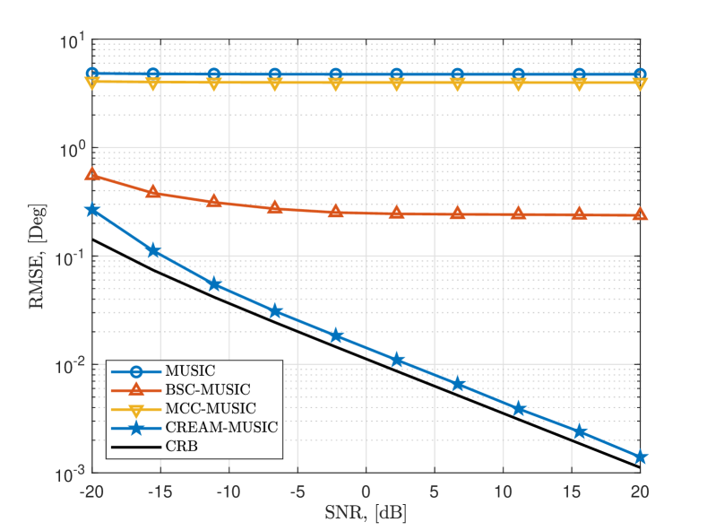
Figure 2: DoA estimation RMSE vs. SNR.

In Fig. 2, we present the DoA estimation RMSE with respect to signal-to-noise-ratio (SNR), which is defined as $\mathrm{SNR}=10\log_{10}(\frac{\rho}{\sigma_{n}^{2}})$, where $\rho=\frac{P_{\mathrm{r}}}{MN^{2}}=1$. As it is seen, both MUSIC and MCC-MUSIC have poor performance because they do not take into account the effect of beam-split. In contrast, BSC-MUSIC exhibits lower RMSE than that of MCC-MUSIC. Specifically, DoA estimation error due to beam-split and MC is approximately $4^{\circ}$ and $0.25^{\circ}$, respectively. The significance of the DoA error due to beam-split is directly related to $\eta_{m}$ (see Fig.1a), which causes deviations in the steering vector model (see (2)). This clearly shows the importance of beam-split compensation. In high SNR, the performance of BSC-MUSIC maxes out due to lose of precision, while the proposed CREAM-MUSIC approach attains the CRB very closely and outperforms the remaining methods yielding poor precision.

V Summary

We examined the THz DoA estimation problem in the presence of beam-split and MC. While the latter has a marginal impact ($\sim 0.25^{\circ}$) on DoA estimation, the former causes significant errors in the array gain and be severe ($\sim 4^{\circ}$). We showed that the proposed CREAM-MUSIC approach can effectively compensate both DoA errors due to beam-split and MC. Furthermore, the proposed method does not require additional hardware components, e.g., time-delayer networks for beam-split calibration.

References

• [1] I. F. Akyildiz, C. Han, Z. Hu, S. Nie, and J. M. Jornet, “Terahertz Band Communication: An Old Problem Revisited and Research Directions for the Next Decade,” IEEE Trans. Commun., vol. 70, no. 6, pp. 4250–4285, May 2022.
• [2] Y. Chen, L. Yan, C. Han, and M. Tao, “Millidegree-Level Direction-of-Arrival Estimation and Tracking for Terahertz Ultra-Massive MIMO Systems,” IEEE Trans. Wireless Commun., vol. 21, no. 2, pp. 869–883, Aug. 2021.
• [3] A. M. Elbir, K. V. Mishra, S. Chatzinotas, and M. Bennis, “Terahertz-Band Integrated Sensing and Communications: Challenges and Opportunities,” arXiv, Aug. 2022.
• [4] H. Sarieddeen, M.-S. Alouini, and T. Y. Al-Naffouri, “An overview of signal processing techniques for Terahertz communications,” Proceedings of the IEEE, vol. 109, no. 10, pp. 1628–1665, 2021.
• [5] S. Venkatesh, X. Lu, H. Saeidi, and K. Sengupta, “A Programmable Terahertz Metasurface With Circuit-Coupled Meta-Elements in Silicon Chips: Creating Low-Cost, Large-Scale, Reconfigurable Terahertz Metasurfaces,” IEEE Antennas Propag. Mag., vol. 64, no. 4, pp. 110–122, Jun. 2022.
• [6] H. Nayir, G. K. Kurt, and A. Görçin, “Angle of Arrival Estimation for Terahertz-enabled Space Information Networks,” in 2022 IEEE Future Networks World Forum (FNWF).   IEEE, Oct. 2022, pp. 153–157.
• [7] B. Zhang, J. M. Jornet, I. F. Akyildiz, and Z. P. Wu, “Mutual Coupling Reduction for Ultra-Dense Multi-Band Plasmonic Nano-Antenna Arrays Using Graphene-Based Frequency Selective Surface,” IEEE Access, vol. 7, pp. 33 214–33 225, Mar. 2019.
• [8] A. Jafargholi, A. Jafargholi, and J. H. Choi, “Mutual Coupling Reduction in an Array of Patch Antennas Using CLL Metamaterial Superstrate for MIMO Applications,” IEEE Trans. Antennas Propag., vol. 67, no. 1, pp. 179–189, Oct. 2018.
• [9] G. Moreno, H. M. Bernety, and A. B. Yakovlev, “Reduction of Mutual Coupling Between Strip Dipole Antennas at Terahertz Frequencies With an Elliptically Shaped Graphene Monolayer,” IEEE Antennas Wirel. Propag. Lett., vol. 15, pp. 1533–1536, Dec. 2015.
• [10] M. Alibakhshikenari, C. H. See, B. S. Virdee, and R. A. Abd-Alhameed, “Meta-Surface Wall Suppression of Mutual Coupling between Microstrip Patch Antenna Arrays for THz-Band Applications,” 2018, [Online; accessed 8. Apr. 2023]. [Online]. Available: https://bradscholars.brad.ac.uk/handle/10454/15908
• [11] J. Tan and L. Dai, “Wideband Beam Tracking in THz Massive MIMO Systems,” IEEE J. Sel. Areas Commun., vol. 39, no. 6, pp. 1693–1710, Apr 2021.
• [12] A. M. Elbir, W. Shi, A. K. Papazafeiropoulos, P. Kourtessis, and S. Chatzinotas, “Terahertz-Band Channel and Beam Split Estimation via Array Perturbation Model,” IEEE Open J. Commun. Soc., p. 1, Mar. 2023.
• [13] A. M. Elbir, K. V. Mishra, S. A. Vorobyov, and R. W. Heath, “Twenty-Five Years of Advances in Beamforming: From convex and nonconvex optimization to learning techniques,” IEEE Signal Process. Mag., vol. 40, no. 4, pp. 118–131, Jun. 2023.
• [14] B. Wang, F. Gao, S. Jin, H. Lin, and G. Y. Li, “Spatial- and Frequency-Wideband Effects in Millimeter-Wave Massive MIMO Systems,” IEEE Trans. Signal Process., vol. 66, no. 13, pp. 3393–3406, May 2018.
• [15] H. Mirzaei and G. V. Eleftheriades, “Arbitrary-Angle Squint-Free Beamforming in Series-Fed Antenna Arrays Using Non-Foster Elements Synthesized by Negative-Group-Delay Networks,” IEEE Trans. Antennas Propag., vol. 63, no. 5, pp. 1997–2010, Feb. 2015.
• [16] A. M. Elbir, “Direction Finding in the Presence of Direction-Dependent Mutual Coupling,” IEEE Antennas Wirel. Propag. Lett., vol. 16, pp. 1541–1544, Jan. 2017.
• [17] A. M. Elbir, K. V. Mishra, and S. Chatzinotas, “Terahertz-Band Joint Ultra-Massive MIMO Radar-Communications: Model-Based and Model-Free Hybrid Beamforming,” IEEE J. Sel. Top. Signal Process., vol. 15, no. 6, pp. 1468–1483, Oct. 2021.
• [18] D. Fan, Y. Deng, F. Gao, Y. Liu, G. Wang, Z. Zhong, and A. Nallanathan, “Training Based DOA Estimation in Hybrid mmWave Massive MIMO Systems,” in GLOBECOM 2017 - 2017 IEEE Global Communications Conference.   IEEE, Dec. 2017, pp. 1–6.
• [19] R. Zhang, B. Shim, and W. Wu, “Direction-of-Arrival Estimation for Large Antenna Arrays With Hybrid Analog and Digital Architectures,” IEEE Trans. Signal Process., vol. 70, pp. 72–88, Oct. 2021.
• [20] A. M. Elbir and S. Chatzinotas, “BSA-OMP: Beam-Split-Aware Orthogonal Matching Pursuit for THz Channel Estimation,” IEEE Wireless Commun. Lett., vol. 12, no. 4, pp. 738–742, Feb. 2023.
• [21] A. M. Elbir, “A Unified Approach for Beam-Split Mitigation in Terahertz Wideband Hybrid Beamforming,” IEEE Trans. Veh. Technol., pp. 1–6, Apr. 2023.
• [22] B. Friedlander and A. J. Weiss, “Direction finding in the presence of mutual coupling,” IEEE Trans. Antennas Propag., vol. 39, no. 3, pp. 273–284, Mar. 1991.
• [23] M. Viberg, M. Lanne, and A. Lundgren, “Calibration in Array Processing,” in Classical and Modern Direction-of-Arrival Estimation.   Cambridge, MA, USA: Academic Press, Jan. 2009, pp. 93–124.
• [24] B. Friedlander and A. J. Weiss, “Direction finding for wide-band signals using an interpolated array,” IEEE Trans. Signal Process., vol. 41, no. 4, pp. 1618–1634, 1993.
• [25] I. Gupta and A. Ksienski, “Effect of mutual coupling on the performance of adaptive arrays,” IEEE Trans. Antennas Propag., vol. 31, no. 5, pp. 785–791, Sep. 1983.
• [26] H. T. Hui, “A practical approach to compensate for the mutual coupling effect in an adaptive dipole array,” vol. 52, no. 5, pp. 1262–1269, May 2004.
• [27] A. M. Elbir and T. E. Tuncer, “Calibration of antenna arrays for aeronautical vehicles on ground,” Aerosp. Sci. Technol., vol. 30, no. 1, pp. 18–25, Oct. 2013.
• [28] A. M. Elbir, “Calibration of directional mutual coupling for antenna arrays,” Digital Signal Process., vol. 69, pp. 117–126, Oct. 2017.
• [29] B. Liao, Z.-G. Zhang, and S.-C. Chan, “DOA Estimation and Tracking of ULAs with Mutual Coupling,” IEEE Trans. Aerosp. Electron. Syst., vol. 48, no. 1, pp. 891–905, Jan. 2012.
• [30] X. Yu, G. Cui, J. Yang, L. Kong, and J. Li, “Wideband MIMO radar waveform design,” IEEE Trans. Signal Process., vol. 67, no. 13, pp. 3487–3501, 2019.
• [31] R. Schmidt, “Multiple emitter location and signal parameter estimation,” IEEE Trans. Antennas Propag., vol. 34, no. 3, pp. 276–280, Mar. 1986.