Quantum readiness for scheduling of Automatic Guided Vehicles (AGVs) as job-shop problem

Abstract

A case study based on a real-life production environment for the scheduling of automated guided vehicles (AGVs) is presented. A linear programming model is formulated for scheduling AGVs with given paths and task assignments. Using the new model, a moderate size instance of $15$ AGVs (all using the same main lane connecting most of the crucial parts of the factory) can be solved approximately with a CPLEX solver in seconds. The model is also solved with a state-of-the art hybrid quantum-classical solver of the noisy intermediate size quantum (NISQ) devices’ era (D-Wave BQM and CQM). It is found that it performs similarly to CPLEX, thereby demonstrating the “quantum readiness” of the model. The hybrid solver reports non-zero quantum processing times, hence, its quantum part contributes to the solution efficiency.

[a]organization=Institute of Theoretical and Applied Informatics, Polish Academy of Sciences, addressline=Bałtycka 5, city=Gliwice, postcode=44-100, country=Poland

[b]organization=Wigner Research Centre for Physics, addressline=Konkoly-Thege Miklós út 29-33., city=Budapest, postcode=1121, country=Hungary

1 Introduction

Modern concepts of production systems require integration (both horizontally and vertically) of all participants in the production process (Hozdić, 2015). Example elements of industry 4.0 include digital twins, automated guided vehicles (AGV) (Luo et al., 2018) or augmented reality (AR) (Stock and Seliger, 2016). AGVs are automatic mobile robots carrying parts and equipment needed during the production process. Many industrial processes can be optimised, including the design of manufacturing systems and processes, assembly line processes, etc. Within these, we address AGV scheduling, in particular, timetabling in a short time horizon. The decisions have to be made almost in real-time, requiring fast computational heuristics.

AGVs can either be autonomous or guided by a central system. The concept of industry 4.0 (Luo et al., 2018) implies that AGV scheduling must be tied to the particular factory specifics. In the present work, we address a problem that arises in a production environment, i.e. the practice of an actual operating factory. (Its identity and further details are confidential.) We model this particular environment, its configuration and requirements, addressing the particular needs of the given factory. In this factory, there is a well-defined space where AGVs can manoeuvre. They are restricted to moving on dedicated "roads" (uni- or bi-directional), reaching ports, loading places, charging stations, etc. Here, the AGVs are controlled by a central system where their scheduling takes place.

In the operation of AGVs, conflicts may arise as many AGVs compete for the use of the “roads”. A conflict is an inadmissible situation when multiple AGVs would run on the same segment of the road network; this would lead to their collision. Thus, it is a basic feasibility requirement against a schedule of AGVs to be conflict-free.

The spatial locations where conflicts are possible are called zones (Ho, 2000). Each zone can be occupied by at most one AGV at a time.

In the standard metaphor of scheduling theory (Pinedo, 2012), zones are machines, and AGVs are jobs. Each AGV has to visit a set of infrastructure elements in a given sequence: each job has to be processed by a set of machines in a prescribed order: this is a job-shop Job Shop ($Jm$) environment. Generalisations allowing for having multiple AGVs in a zone would result in Flexible Job Shop ($FJc$) environment; this we will not consider here. We treat parts of the infrastructure that lie between zones (i.e. where conflicts are not expected) as buffers. The requirement of a minimal headways between AGVs leaving and entering zones and deadlock constraints on bi-directional "roads" (also termed as lanes) imply blocking constraints ($block$). The prescription of the initial availability of AGVs implies release date ($r_{j}$) constraints. the passing times of AGVs given through particular resource is limited. Hence, processing times ($p_{im}$) appear. In addition, due dates ($d_{i}$) are also prescribed: the AGVs’ tasks have to be completed in a given time. Finally, permutation ($prmu$) constraints arise as AGVs cannot overtake on lanes between zones. Recirculation ($rcrc$), that is, if a given AGV can visit the same zone multiple times during the trip, could also considered but will not be addressed here as it does not occur in the particular factory we model.

As for the objective, the goal is to ensure that the AGVs finish their travels as soon as possible, taking into account certain priorities, too. Hence, the objective is the travel completion time, the weighted sum of completion times of each AGV. We shall refer to this as completion time in what follows. Altogether, with the standard notation of scheduling theory, our problem falls in the class $(J_{m}|r_{j},p_{im},d_{i},block,prmu|\sum_{j}w_{j}C_{j})$.

The planning of AGVs’ paths and task assignment, which is widely analysed along with scheduling in literature (as reviewed by Zhong et al., 2020), is not part of our optimisation task. We are required to address AGV scheduling in itself, which has less coverage in the literature. This particular optimisation problem appears to be complex but still tractable for the meaningful number of AGVs ($15$ AGVs in particular). When considering more, e.g. $40$ AGVs in a factory in a limited space, solving the problem on time can become problematic with certain heuristics. Hence, new heuristics or computational paradigms may be necessary for such future applications.

A possible choice for a new paradigm can be quantum computing, offering improved efficiency in certain cases of computational problems (Preskill, 2012). It is widely recognised that we are in the era of noisy intermediate-scale quantum devices (Preskill, 2018; Brooks, 2019): a few hundred quantum bits are technologically available, but noise and imperfections still have a relevant impact on their operation. In spite of that, the first examples of quantum supremacy have already been presented by (Arute et al., 2019), and there is an increasing research interest in potential industrial applications that are considered, (see, e.g. Domino et al., 2023; Vikstål et al., 2020; Geitz et al., 2022). The size and characteristics of the AGV scheduling problem addressed in this paper make it a good candidate to further explore noisy-intermediate scale quantum (NISQ) technologies in industrial applications. Here, we present a model meeting the requirement of the aforementioned production environment and solve it using proprietary hybrid quantum-classical solvers. We find that the performance of these is similar to that of CPLEX, thereby demonstrating the “quantum readiness” of our model.

This paper is organised as follows. In Section 2 we present a brief review of the literature of AGV scheduling. In Section 3, we define our problem and formulate it as an integer linear programming (ILP) model. In Section 4 we transform the model also to a quadratic unconstrained binary optmization (QUBO) problem which is the native form of a problem that quantum annealers address. In Section 5 we discuss computational results. In Section 6, we draw conclusions, while Appendix Appendix is devoted to additional details.

2 Literature review

In the broad picture of production scheduling, (Rossit et al., 2019) describes a currently promising approach as Smart Scheduling that combines the cyber-physical production systems (CPPS) with the decision support system (DSS). The AGV scheduling optimisation can be treated either as part of the larger industrial system in light of the philosophy of industry 4.0 (Stock and Seliger, 2016) (e.g. together with industrial job scheduling) or just as a sole component. For the sake of demonstration, we concentrate on the latter. However, our model can be re-integrated into a general DSS system.

According to Zhong et al. (2020); Qiu et al. (2002), AGV scheduling algorithms are divided into rostering and routing. The aim of rostering is to dispatch a set of AGVs to perform certain jobs of equipment transportation within the factory. Then, routing (path planning) aims at finding suitable paths for the AGVs, together with the ”timetable” and a possible ordering of AGVs passing certain congested places. These problems are commonly solved via linear programming optimisation (see, e.g. the works of Qiu et al., 2002; Vivaldini et al., 2015). As already declared, here we concentrate on a particular part of this series of planning processes: scheduling.

Le-Anh (2005) provides a fair overview of the optimisation of AGVs scheduling. Vehicle rostering is discussed both as an offline scheduling problem (where all transportation requests are known in advance) or online scheduling (where environments are stochastic and requirements appear on the fly, c.f. the work of Sabuncuoglu and Bayız (2000)). We follow the approach of deterministic offline scheduling, but each time the circumstances change, we recalculate schedules. An important constraint (tied to due time constraints in scheduling theory) is the maximal window of time in which a task has to be performed by an AGV. The objective is a linear function of variables reflecting completion time costs. To solve both static and dynamic problems, most authors apply integer linear programming (ILP) together with a (custom) column generation approach and various methods of optimisation. As we consider routes and tasks of AGVs predefined for our optimisation problem, column generation is not applicable.

An important issue with AGVs is the possibility of deadlocks, where several AGVs come to such a point that none of them can move forward because each of them is blocked by the others. Le-Anh (2005) mentions various deadlock resolution methods:

1. Balancing the system workload, i.e. using workload-related dispatching rule (Kim et al., 1999),

2. Controlling the traffic at intersections by semaphores (Evers and Koppers, 1996),

3. Introducing static or dynamic zones that can be occupied by a limited number of AGVs for a dynamic-zone strategy for vehicle-collision (Ho, 2000) prevention.

These deadlock resolution strategies can mostly be encoded as constraints to the ILP. We have opted for the last approach, i.e. dynamic zones.

The literature of bigger-scale AGV scheduling problems is still scarce and the considered sizes are rather limited when comparing to industry practice. For instance, in a recent paper Li et al. (2019) consider a system with $9$ AGVs already as a large-scale one. We opt for quantum computing methods in the hope that a quantum-ready model can potentially scale better than classical computer algorithms. Hence, the development of quantum hardware may open the possibility of dealing with really large problem instances efficiently. In particular, we will use quantum annealing, which is part of an adiabatic model of quantum computation (Kadowaki and Nishimori, 1998; Farhi et al., 2000).

Our research is not the first of this kind, but it shows marked differences from the others. Our approach is complementary to the one presented by Geitz et al. (2022), where the job scheduling in a factory is optimised on a quantum annealer or classical device. There, however, the focus is on the factory machines. As opposed to that, we focus on the AGV traffic, assuming job assignments to industrial machines are fixed. Haba et al. (2022) also addressed a problem of AGV scheduling with quantum methods. There, however, quantum annealing was applied for the routing of AGVs, as opposed to our problem, which addresses the timing and ordering of the AGVs.

3 Model formulation

As mentioned before, we concentrate on certain components of AGVs scheduling; AGVs’ timing and ordering in particular. The objective is the weighted sum of completion times (Le-Anh, 2005), the weights reflect the priorities of AGVs. We assume that AGVs’ tasks and paths (represented by the colour lines in Fig. 1) are pre-defined as input of our problem. Each time these inputs are changed, a new optimisation problem is created and recomputed. Such changes in the input can be caused e.g. by disturbances in the AGV traffic.

3.1 Problem introduction

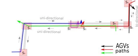
Figure 1: Example of the AGV scheduling problem given pre-defined AGVs paths as colour lines. Zones $s_{0},\ldots s_{6}$ are spatial areas where AGVs paths intercept start or end. AGVs paths in terms of zones are AGV $s_{0},s_{1},s_{2},s_{3}$, AGV $s_{4},s_{3},s_{2},s_{1}$, AGV $s_{6},s_{5},s_{4},s_{3}$ $AGVs_{5},s_{6}$ and AGV $s_{2},s_{3}$

Fig. 1 displays an example of the considered topologies. This setup closely resembles the situation in the considered real-life factory (it is distorted to maintain confidentiality). AGVs paths (colour lines) are as follows:

• bi-directional lanes (e.g. between $s_{5}$ and $s_{6}$ in Fig. 1),

• uni-directional lanes,

• zones (c.f. Ho, 2000) the locations where conflicts are possible according to the given (predefined) paths, i.e. where AGVs paths split, join or where uni-directional lanes start or end.

To avoid collisions, we assume that one AGV can occupy each zone at a time. Hence, zones can be treated as machines in Job Shop problem. (This limitation can be lifted in a more elaborate model by increasing the allowed number of AGVs within the zone and introducing some local traffic conditions (Evers and Koppers, 1996).)

The practical AGVs scheduling will be performed via the following algorithm triggered at each change of input parameters.

Fixed inputs

1. $\mathcal{J}$ - set of AGVs;

2. $w_{j}$ - priority weights (as the part of total weighted completion time objective);

3. $d_{\max}$ - the parameter determining the time window, due time can be computed form this parameter;

4. topology of the network as in Fig. 1, containing:

   • uni-directional double lanes,

   • bi-directional single lanes (imposing blocking constraints);

5. minimal headways between two subsequent AGVs, this is a parameter of blocking constraints.

Variable inputs

1. starting points of AGVs in time and space,

2. AGVs destinations and paths (from this, the sequence of machines will be determined);

3. nominal speeds of AGVs, processing time constraints can be formulated based on these parameters.

Processing

1. from paths of AGVs create zones where conflicts are possible; see Fig. 1,

2. define AGVs paths by the sequence of zones e.g. $S_{j}=\{s_{j,1},s_{j,2}\ldots s_{j,\text{end}-1},s_{j,\text{end}}\}$, e.g. see caption of Fig. 1;

3. given initial conditions, compute the lowest possible entering and leaving times of each AGV at the zones, assuming there are no collisions between the given AGV and all other AGVs;

4. encode problem into ILP: entering and leaving times of AGVs at the zones are integer decision variables, and there are binary precedence variables determining which AGV leaves a zone first. (A relaxation of the integer constraint on time variables, yielding a mixed integer program is also meaningful but not considered here as quantum devices support integers. In addition, our computational experience shows that the relaxation of the integer constraints on time variables and using a MILP solver does not lead to a significant improvement in computational time when using CPLEX; the real difficulty is encoded in the precedence variables.) Lower limits of these variables are determined in point $3$ while upper limits are determined by lower limits and model parameter $d_{\text{max}}$, encode constraints and objective;

5. solve the problem using a chosen solver (classical, quantum, hybrid, etc.).

Output

1. conflict-free timetable of AGVs encoded as entering and leaving times of AGVs at zones, or correspondingly the precedence of AGVs therein.

Points $1$ - $4$ in processing are pre-processing steps. The higher computational effort is required in point $5$, which deals with optimisation. Hence, the efficiency comparisons will refer only to point 5 of the algorithm.

3.2 Encoding the problem into an ILP

Here we provide the details of the model in step 4 of the processing phase of the algorithm.

Decision variables include the integer times when AGVs are entering and leaving zones are denoted by $t_{\text{in / out}}(j,s)$. As floating point numbers cannot be treated easily, we use integer time variables $t_{\text{in / out}}(j,s)\in\mathbb{N}$, with minute  todocheck resolution. The time window constraints (Le-Anh, 2005), imply that each of these variables to fit into the time window of length $d_{\max}$, namely:

$$\upsilon_{\text{in / out}}(j,s)\leq t_{\text{in / out}}(j,s)\leq\upsilon_{\text{in / out}}(j,s)+d_{\text{max}}.$$ (1)

where $\upsilon_{\text{in / out}}(j,s)$ are lower limits computed by assuming the nominal speed of $j$’th AGV and assuming no conflicts (collisions) with other AGVs, according to Pinedo (2012) the $d_{\max}$ parameter imposes due time constraints, while lower limits are tied to release date constraints. Let $|\mathcal{S}|$ be the number of zones in a particular optimisation problem, and $|\mathcal{J}|$ the number of AGVs therein. To count the number of $t$ variables in Eq. (1), observe that if an AGV passes a zone, there are two such variables (that is, entering and leaving times). Then

$$\#t\leq 2|\mathcal{J}||\mathcal{S}|,$$ (2)

inequality is because not all AGVs pass through all zones.

To determine the order of AGVs at zones we intoduce binary precedence variables.

• For zone $s$ passed by AGVs $j$ and $j^{\prime}$ we have:

  $$y_{\text{in}/\text{out}}(j,j^{\prime},s)\in\{0,1\}$$ (3)

  which is equal to $1$ iff $j$ enters / leaves zone $s$ before $j^{\prime}$, as the order of AGVs can not be changed at the zone; obviously:

  $$y_{\text{in}/\text{out}}(j,j^{\prime},s)=1-y_{\text{in}/\text{out}}(j^{\prime},j,s).$$ (4)

• For a bi-directional lane (joining zones $s$ and $s^{\prime}$) used by AGV $j$ heading in one direction and AGV $j^{\prime}$ heading in opposite direction, we assign the following precedence variable:

  $$z(j,j^{\prime},s,s^{\prime})\in\{0,1\},$$ (5)

  which is equal to $1$ iff $j$ enters such lane (bounded by zone $s$ and $s^{\prime}$) before $j^{\prime}$, and zero otherwise, hence,

  $$z(j,j^{\prime},s,s^{\prime})=1-z(j^{\prime},j,s^{\prime},s).$$ (6)

For each pair of AGVs passing a zone, we have two precedence variables ($y_{in}$ and $y_{out}$), therefore

$$\#y\leq|\mathcal{J}|\left(|\mathcal{J}|-1\right)|\mathcal{S}|.$$ (7)

(It is an inequality is because not all pairs of AGVs pass through all zones.) If the whole topology consists of the bi-directional lanes we have $\#z=\#y$. It is obviously not true if some of the lanes are uni-directional; then we have:

$$\#z\leq\#y\leq|\mathcal{J}|\left(|\mathcal{J}|-1\right)|\mathcal{S}|.$$ (8)

Objective is defined as the weighted sum of completion times (see Le-Anh, 2005), namely:

$$f=\sum_{j\in\mathcal{J}}w_{j}\frac{t_{\text{out}}(j,s_{j,\text{end}})}{d_{\text{max}}}.$$ (9)

where $s_{j,\text{end}}$ is the last zone of the path of $j$ AGV, and $w_{j}$ is the weight tied to priority of such AGV. (We assume that after leaving the last zone the AGV’s path is conflict-free.) This can be referred to as the total completion time objective.

Constraints. The minimal passing time constraint (mpt) of AGVs between subsequent zones can be computed from the problem topology and AGVs speeds. For any pair of subsequent zones $(s,s^{\prime})$ on the route of AGV $j$ we require:

$$t_{\text{in}}(j,s^{\prime})\geq t_{\text{out}}(j,s)+\tau^{\text{pass}}(j,s,s^{\prime}),$$ (10)

see Fig. 2 (upper panel). In our model zones are considered as bottle-neck areas, hence we allow waiting of AGVs in the buffer, before the zone entrance, yielding $\geq$ sign in Eq. (10). There is one such inequality in for each AGV and each zone it passes. Then, taking upper limit of each AGV passing each zone we have:

$$\#_{\text{mpt}}\leq|\mathcal{J}||\mathcal{S}|$$ (11)

The minimal headway constraint (mh) is the model input, that determines minimal time spacing between two subsequent AGVs. In detail, consider two AGVs $j,j^{\prime}$ heading in the same direction. Let $s*,s,s^{\prime}$ be the sequence of subsequent zones they both pass. Then:

$$t_{\text{out}}(j^{\prime},s)+M\cdot y_{out}(j^{\prime},j,s)\geq t_{\text{out}}(j,s)+\tau^{\text{headway}}(j,j^{\prime},s,s^{\prime}),$$ (12)

see Fig. 2 (lower panel), and analogically

$$t_{\text{in}}(j^{\prime},s)+M\cdot y_{in}(j^{\prime},j,s)\geq t_{\text{in}}(j,s)+\tau^{\text{headway}}(j,j^{\prime},s^{*},s).$$ (13)

Here $M$ is a large enough number for inequality to always hold for $y(j^{\prime},j,s)=1$. If $s$ does not have a successor in the sequence, we do not consider Eq. (12). Analogically, if $s$ does not have the predecessor, we do not consider Eq. (13). The minimal headway (mh) constraint is required for each pair of AGVs following each other at each zone. There are roughly $\frac{|\mathcal{J}|^{2}}{2}$ such pairs if we assume that half of AGVs are going in one way and half going in the other way. For the upper limit (under this assumption), we consider all AGVs passing all zones. Then for each AGV in the pair and each zone, we have one constraint from Eq. (12). and one constraint form Eq. (13), yielding:

$$\#_{\text{mh}}\leq 2\frac{|\mathcal{J}|^{2}}{2}|\mathcal{S}|=|\mathcal{J}|^{2}|\mathcal{S}|.$$ (14)

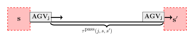
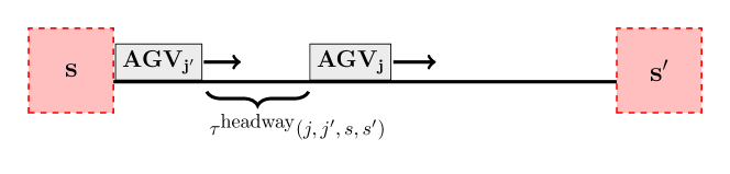
Figure 2: Illustration of minimal passing time (upper panel) and headway (lower panel) Eq. (10)

The deadlock on bi-directional lane constraint (d) is defined as follows. Let the pair $(s,s^{\prime})$ be two zones connected by the single bi-directional lane and $j$ and $j^{\prime}$ be two AGVs first going $s\rightarrow s^{\prime}$ and the second $s^{\prime}\rightarrow s$. Then:

$$t_{\text{out}}(j^{\prime},s^{\prime})+M\cdot z(j^{\prime},j,s^{\prime},s)\geq t_{\text{in}}(j,s^{\prime})$$ (15)

and

$$z(j,j^{\prime},s,s^{\prime})=y_{in}(j,j^{\prime},s)=y_{in}(j,j^{\prime},s^{\prime})$$ (16)

Eq. (16) yields that the order of AGVs heading in opposite directions can not change between zones $s$, $s^{\prime}$, as they can not meet at bi-directional lane which would lead to the deadlock. Assuming, as before, that half of AGVs were going there in one direction and half in the other, we would expect from Eq. (15):

$$\#_{\text{d}}\leq|\mathcal{J}|^{2}|\mathcal{S}|.$$ (17)

It s an equality if all lanes are bi-directional and all AGVs pass all zones. Referring to Eq. (14) and Eq. (17) we expect then:

$$\#_{\text{mh}}+\#_{\text{d}}\leq 2|\mathcal{J}|^{2}|\mathcal{S}|.$$ (18)

We assume that the zone can be occupied only by one AGV at the time. This is to avoid collisions within the zone. Hence AGV $j^{\prime}$ can enter the zone after $j$ leaves it (provided $j$ is first on the zone, i.e. $y_{in}(j^{\prime},j,s)=0$):

$$t_{\text{in}}(j^{\prime},s)+M\cdot y_{in}(j^{\prime},j,s)\geq t_{\text{out}}(j,s)$$ (19)

Then we also have to include minimal passing time over the zone $\tau^{\text{zone}}$

$$t_{\text{out}}(j,s)\geq t_{\text{in}}(j,s)+\tau^{\text{zone}}(j,s).$$ (20)

We prescribe the upper limit of all AGVs passing all zones. Then for each zone and each AGV we have $|J|-1$ inequalities from Eq. (19) and one inequality from Eq. (20), yielding:

$$\#_{\text{zc}}\leq|\mathcal{J}|^{2}|\mathcal{S}|.$$ (21)

In the language of sceheduling theory, the assumption that the zone can be occupied by one AGV only defines the JobShop machine environment, and the prescription of the passing time over zones imposes processing time constraints.

As AGVs are, in general, moving with similar speed, we assume that they can not overtake both on lanes and zones. This no overtake (no) constraint requires the order of such AGVs to be maintained. (This is the permutation constraint in the language of scheduling theory.) In detail, let $j$ and $j^{\prime}$ be a pair of AGVs heading in the same direction, passing the sequence of zones: $s_{1},s_{2},\ldots s_{k}$. Then:

$$y(j,j^{\prime},{s_{1}}_{out})=y(j,j^{\prime},{s_{2}}_{out})=\ldots=y(j,j^{\prime},{s_{k}}_{out})$$ (22)

(Note that if the route of two AGVs splits and joins later, the condition in Eq. (22) has to be modified). We have

$$\#_{\text{no}}\leq\frac{|\mathcal{J}|^{2}|\mathcal{S}|}{2}$$ (23)

such equailities. As mentioned before, we also assume that AGVs can not overtake within a zone:

$$y_{in}(j,j^{\prime},s)=y_{out}(j,j^{\prime},s).$$ (24)

Number of variables and constraints

Assuming that the constraints in Eq. (24) always hold (and cannot be lifted in our model), we have one $y$-variable (and $z$-variable) per zone, thus Eqs. (7)  (8) yield:

$$\begin{split}\#y\leq\frac{|\mathcal{J}|\left(|\mathcal{J}|-1\right)|\mathcal{S}|}{2},\\ \#z\leq\frac{|\mathcal{J}|\left(|\mathcal{J}|-1\right)|\mathcal{S}|}{2}\end{split}$$ (25)

Then, referring to Eq. (2) we can assume

$$\#y+\#z+\#t\ll|\mathcal{J}|\left(|\mathcal{J}|-1\right)|\mathcal{S}|+2|\mathcal{J}||\mathcal{S}|.$$ (26)

For topologies with most uni-directional lanes (as in our example discussed later), then $\#z\ll\#y$, and therefore

$$\#y+\#z+\#t\ll\frac{|\mathcal{J}|\left(|\mathcal{J}|-1\right)|\mathcal{S}|}{2}+2|\mathcal{J}||\mathcal{S}|.$$ (27)

Recall that $t$ are integer variables that can take $d_{\max}+1$ values, while $y$ and $z$ are binary variables.

Let us now estimate the number of inequalities. The number of minimal passing time (mpt) constraint inequalities (see Eq. (11) ) is linear in $|\mathcal{J}|$, while the number of inequalities form all other constraints (zc, mh, d) is quadratic n $|\mathcal{J}|$. Finally, for a large number of AGVs, we can assume the:

$$m=\#_{\text{mpt}}+\#_{\text{zc}}+\#_{\text{mh}}+\#_{\text{d}}\approx\#_{\text{zc}}+\#_{\text{mh}}+\#_{\text{d}}\leq 3|\mathcal{J}|^{2}|\mathcal{S}|,$$ (28)

see Eqs. (17), (21). We can conclude, then, that the problem scales linealy in the number of zones $|\mathcal{S}|$ and quadratically in the number of AGVs $|\mathcal{J}|$. The quadratic scaling can cause difficulties whhen applying the model to a large number of AGVs.

4 Transformation of ILP to QUBO

Quantum annealing processors (such as the D-Wave machine) input problems in the Ising form

$$\min_{(s_{1},\ldots s_{n})\in\{-1,1\}^{N}}\sum_{(i,j)\in E}s_{i}J^{\prime}_{i,j}s_{j}+\sum_{i\in V}s_{i}h^{\prime}_{i}$$ (29)

where $s_{i}$ are spin variables $s_{i}\in\{-1,1\}$, and parameters are $J^{\prime}_{i,j}$ i.e. couplings between spins, $h^{\prime}_{i}$ - local fields. To transform the aforementioned ILP into Ising, in an intermediate step, the problem is encoded as Quadratic Unconstrained Binary Optimization (QUBO) problem, namely:

$$\min_{(x_{1},\ldots x_{n})\in\{0,1\}^{N}}\sum_{(i,j)\in E}x_{i}J_{i,j}x_{j}+\sum_{i\in V}x_{i}h_{i}$$ (30)

where $x_{i}\in\{0,1\}$ are binary variables, and $s_{i}=2x_{i}-1$.

To transform the ILP into the QUBO, we use the Binary Quadratic Model (BQM) transformation implemented in the Python dimod library. The most general form of inequalities in our model is in Eq. (12) or Eq. (13). We will demonstrate the transformation of ILP to QUBO on the example of these equations; the same procedure is applied to the others.

Let us contract $t$-variables and $y$-variables to vectors with elements $t_{j}$ and $y_{i}$ (the same with constant terms $c_{i}$). Then from Eq. (12) or Eq. (13) we have terms in the form

$$t_{j}-t_{j^{\prime}}-My_{i}+\xi_{i}=-c_{i}.$$ (31)

To replace inequalities with equities, we use slack variables

$$0\leq\xi_{i}\leq\bar{\xi}_{i}.$$ (32)

For Eq. (12), it can be demonstrated that

$$\bar{\xi}_{i}=-\min(t_{j}-t_{j^{\prime}}-My_{i})-c_{i}=-\upsilon_{j}+\upsilon_{j^{\prime}}+d_{\max}+M_{i}-c_{i}=d_{\max}+M_{i},$$ (33)

as $\min(t_{j})=v_{j}$, and $\max(t_{j})=v_{j}+d_{\max}$ from Eq. (1), and we expect $\upsilon_{j^{\prime}}=\upsilon_{j}+c_{i}$. Here we have $d_{\max}+M_{i}+1$ distinct values of slack variable $\xi_{i}$. Some of the inequalities such as the minimal passing time constraints in Eq. (10) lack precedence variables ($y$ or $z$). Thus we expect $\bar{\xi}_{i}=d_{\max}$.

To turn the constrained problem in Eq. (31) into the unconstrained one, we use the penalty method: the $i$th constraint violation is penalized by the hard constraint penalty $p>0$. Such a penalty has to be sufficiently large not to be overruled by the objective. Then, we have

$$\begin{split}\textrm{min.}_{t_{1},\ldots,y^{\prime}_{1},\ldots,\xi_{1},\ldots}\ \ p\sum_{(j,j^{\prime},i)\in\mathcal{I}}({t_{j}-t_{j^{\prime}}-M_{i}y^{\prime}_{i}+\xi_{i}+c_{i})^{2}}+p\sum_{(i,i^{\prime})\in\mathcal{I^{\prime}}}(y^{\prime}_{i}-y^{\prime}_{i^{\prime}})^{2}+\text{objective}.\end{split}$$ (34)

The first sum is for following constraints: (mpt) Eq. (10), (mh) Eqs. (12), (13), (d) Eq. (15) (zc) Eqs. (19) (20), and takes $M_{i}=0$ if no precedence variable is included, the set $\mathcal{I}$ contains all indices tied to these constraints, yielding $|\mathcal{I}|=m$ (c.f. Eq. (28)). The number of slack variables is also equal to $m$, as we have one slack variable per inequality. The second sum is for equates of precedence variables in (no) constraint Eq. (28) and (d) constraint in Eq. (16). Then, $\mathcal{I^{\prime}}$ contains all indices tied to this constraint, and $|\mathcal{I^{\prime}}|=\#_{\text{no}}+\#_{\text{d}}$.

Finally (following Eq. (5) in (Karimi and Ronagh, 2019)) , we replace all $t_{i}$ and $\xi_{i}$ with the corresponding monomial of bits $\sum_{k}d_{k}b_{k}$ where $b_{k}$ are new bits variables. This transforms the quadratic unconstrained model into the quadratic unconstrained binary model. We have $\#t$ t-variables (with $d_{\max}+1$ distinct values) and $m$ slack variables (with at most $d_{\max}+\tilde{M}+1$ distinct values), where $\tilde{M}=\max_{i}\xi_{i}$. Using Eq. (28), the number of binary variables in QUBO representation can be limited by

$$\#\text{QUBO}\leq\#t\big{\lceil}\ln_{2}(d_{\text{max}}+1)\big{\rceil}+m\big{\lceil}\ln_{2}(d_{\text{max}}+\tilde{M}+1)\big{\rceil}+\#y+\#z.$$ (35)

The size of the problem scales linearly the number of zones and quadratically in the number of AGVs. The number of constraints per variable (the mean vertex degree of the graph model) is tied to the expansion of quadratic terms in Eq. (34).

5 Computational results

For numerical calculations we used examples of problems similar to those presented in Fig. 1, but with different numbers of AGVs and zones where collisions may occur. This is a typical setting for an industrial system, as various AGVs are in traffic at various time moments, and collision zones form dynamically. For the particular parameter setting in the example case of $7$ zones, see Fig. 3 - yielding a rather typical industrial situation. The particular values of parameters can be read out from the topology, AGVs speeds and zone locations. The particular example of $7$ zones and $7$ AGVs is discussed in detail in the Appendix.

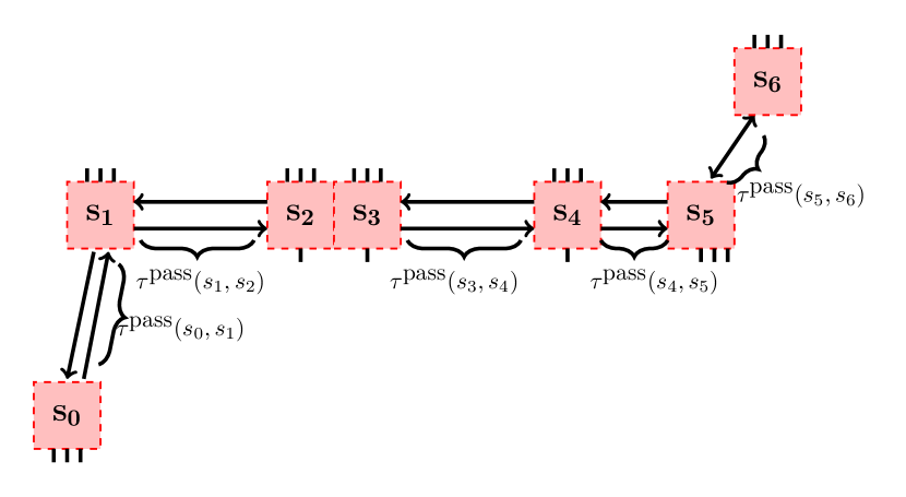
Figure 3: Example network with $7$ zones derived from Fiq. 1

Importantly, the results of optimisation and values of precedence variables, in particular, can be plugged into the application programming intefrace (API) of the industrial system, uniquely defining the order of AGVs at each zone while the traffic beyond zones is conflict-free. From an optimisation point of view, one of our goals is to examine the scaling of the problems’ computational time and number of variables and constraints with the size of the problem in terms of $|\mathcal{J}|$ and $|\mathcal{S}|$ (namely the number of AGVs and zones). We start with $2$ AGVs and $4$ zones in Tab. 1, and end with $15$ AGVs and $7$ zones in Tab. 6. In all cases we have recorded the small but non-zero computational time recorded on both hybrid solvers. From this we can conclude that quantum component contributed to the efficiency of the computation.

	classical CPLEX	hybrid CQM solver	hybrid BQM solver	quantum D-Wave
is feasible	yes	yes	yes	no
ground state	yes	yes	no	no
n.o. broken constraints	$0$	$0$	$0$	$4$
objective	$4.0$	$4.0$	$4.7$	-
comp time	$0.0074$ s	$5.01$ s	$2.98$ s	$1$ s
QPU time	-	$31813\,\mu$s	$38242\,\mu$s	$250\,\mu$s per run

Table 1: Solution of $2$ AGV and $4$ zones problem with $d_{\max}=10$.

	classical CPLEX	hybrid CQM solver	hybrid BQM solver	quantum D-Wave
is feasible	yes	yes	no	no
ground state	yes	yes	no	no
n.o. broken constraints	$0$	$0$	$4$	$10$
objective	$8.2$	$8.2$	-	-
comp time	$0.016$ s	$5.01$ s	$2.98$ s	1 s
QPU time	-	$32019\,\mu$s	$42677\,\mu$s	$250\,\mu s$

Table 2: Solution of $4$ AGVs and $5$ zones problem with $d_{\max}=10$.

	classical CPLEX	hybrid CQM solver	hybrid BQM solver	quantum D-Wave
is feasible	yes	yes	no	x
ground state	yes	yes	no	x
n.o. broken constraints	$0$	$0$	$25$	x
objective	$3.22$	$3.22$	-	x
comp time	$0.016$ s	$5.01$ s	$3$ s	x
QPU time	-	$16040\,\mu$s	$42655\,\mu$s	x

Table 3: Solution of $6$ AGV and $7$ zones problem, $d_{\max}=40$.

	classical CPLEX	hybrid CQM solver	hybrid BQM solver	quantum D-Wave
is feasible	yes	yes	no	x
ground state	yes	yes	no	x
n.o. broken constraints	$0$	$0$	$43$	x
objective	4.25	4.25	-	x
comp time	$0.031$ s	$5.01$ s	$3.4$ s	x
QPU time	-	$16050\,\mu$s	$85298\,\mu$s	x

Table 4: Solution of $7$ AGV and $7$ zones problem with $d_{\max}=40$.

	classical CPLEX	hybrid CQM solver	hybrid BQM solver	quantum D-Wave
is feasible	yes	yes	no	x
ground state	yes	no	no	x
n.o. broken constraints	$0$	$0$	$280$	x
objective	$9.175$	$9.25$	-	x
comp time	$49.05$ s	$5.01$ s	$2.98$ s	x
QPU time	-	$32031\,\mu$s	$170609\,\mu$s	x

Table 5: Solution of $12$ AGVs and $7$ zones problem with $d_{\max}=40$.

	classical CPLEX	hybrid CQM solver	hybrid BQM solver	quantum D-Wave
is feasible	yes	yes	no	x
ground state	yes	no	no	x
n.o. broken constraints	$0$	$0$	$310$	x
objective	$10.975$	$11.32$	-	x
comp time	$378.84$ s	$5.01$ s	-	x
QPU time	-	$32035\,\mu$s	$170604\,\mu$s	x

Table 6: Solution of $15$ AGVs and $7$ stations problem with $d_{\max}=40$.

The quantum annealing on the D-Wave machine can be performed only on small problems (up to $4$ AGVs) because of the limitation of the size of the annealer (number of qubits and couplings). Furthermore, the obtained solutions are not feasible due to the imperfection of the annealer. This observation gave us the motivation to apply hybrid quantum-classical solvers. We used two hybrid solvers supplied by the D-Wave company: BQM and CQM (D-Wave Systems Inc., 2022b, a). The BQM solver inputs QUBO problems, as described in Section 4, and solves them with a portfolio of classical heuristics. In the course of the process, certain subproblems are sent to the quantum processor. In the cas of the CQM solver the input is an ILP and its transformation to QUBO is performed within the solver. These solvers are proprietary and closed source; their details are hidden to the users. Nevertheless, the schematic data flow in these solvers is summarised in Fig.$5$ in DWave’s whitepaper (D-Wave Systems Inc., 2022b). In particular, the data flow is describe as follows. The solver reads the input problem, either as a constrained quadratic model (CQM) or QUBO (BQM). Then, it invokes the number of heuristic solvers that run in parallel using classical CPUs and GPUs and search for good quality solutions for the given problem. Each of these heuristics has the Quantum Module (QM) that can send queries to QPU. Its responses to these queries are used to guide the heuristic search or to improve the quality of a current pool of solutions. After postprocessing (removing duplicates, etc.), the subset of results is forwarded to the user.

In our examples, the BQM solver did not return high-quality solutions for larger sizes of the problem. Notably, the solutions were not feasible. This suggests that our ad-hoc choice of the penalty coefficients should be replaced by a more advanced and systematic choice. The question of the right choice of penalties is indeed a nontrivial problem, see e.g. the works of Karimi and Ronagh (2017) or Gusmeroli and Wiegele (2022). This can be a subject for a future research. Meanwhile, the CQM hybrid solver always provided feasible solutions, hence it is not necessary to address the question of penalties in our practical situation. In terms of computational time CQM has outperformed the classical exact CPLEX solver for large problems ($12$ and $15$ AGVs). The CQM hybrid solver is approximate heuristic, and the provided solutions, although feasible, had a slightly higher objective value than the exact solution. Henceforth, to be fair, the CQM solver will be compared with an approximate CPLEX solution further on. In Tab. 7, the CQM hybrid solver is compared with other solvers, including the approximate CPLEX solver. This overview shows that the CPLEX approximate solver performing all computations in $1$ second, is fast enough for almost online scheduling and dynamics response of our algorithm. Hence, such results would be admissible for practical application in real-life factory. The results with CQM solver are competitive and illustrate an efficient application of hybrid algorithms. In the future, when better quantum annealers will be available, they may become more efficient than classical heuristics.

$|\mathcal{J}|$ / $|\mathcal{S}|$	CPLEX exact		CPLEX approx Branch & Bound		D-Wave hybrid CQM
	comp. time [s]	objective / optimal	comp. time [s]	objective / optimal	comp. time [s]	objective / optimal
2 / 4	0.0074	1	1	1	5.01	1
4 / 4	0.016	1	1	1	5.01	1
6 / 7	0.016	1	1	1	5.01	1
7 / 7	0.031	1	1	1	5.01	1
12 / 7	49.05	1	1	1	5.01	1.008
15 / 7	378.84	1	1	1.002	$5.01$	1.03

Table 7: Comparison of performance of Classical CPLEX exact and approximate with hybrid quantum-classical solver CQM (approximate). All solutions were feasible.

For the problem of $15$ AGVs and $7$ zones, the problem is still tractable using classical heuristics. But, referring to upper limits of problem size Eqs. (27) (28) (23), here the size of the problem scales quadratically with the number of AGVs. For the $15$ AGVs and $7$ zones problem we have $696$ variables (upper limit according to Eq. (27) was $945$), and $1378$ linear constraints (upper limit according to Eq. (23) (28) was $5513$). These limits are quadratic in the number of AGVs, and linear in the number of zones. We may expect the problem size to be quadratic with the number of AGVs as the number of zones is constant. If, however, the number of AGVs increases further, more zones will appear where collisions occur and therefore the problem size will scale worse than quadratic.

6 Conclusions

In this research, we have demonstrated “quantum readiness” for close to real-life AGVs scheduling problem, that can be implemented in a real factory environment. We have not yet demonstrated quantum supremacy, but still, the results of one of the hybrid quantum-classical approaches are close to the ones of CPLEX. As such hybrid approaches are expected to improve in the near future, we may be on the edge of quantum supremacy. Larger problems of hundreds of AGVs may remain out of range for classical algorithms, while future hybrid quantum-classical algorithms may potentially demonstrate their utility.

Data availability

The code and the data used for generating the numerical results can be found in https://github.com/iitis/AGV_quantum

Appendix

In the Appendix, we present a step-by-step solution of the $7$ AGVs and $7$ zones problem with topology presented in Fig 3. (In practice, zones will be determined dynamically before optimisation in point $1$ of the algorithm). We have bi-directional lanes between zones $s_{0}$, $s_{1}$, $s_{2}$, $s_{3}$, $s_{4}$ and $s_{5}$ as well uni-directional lane between zones $s_{5}$ and $s_{6}$. For this particular computation, the following parameters have been chosen: $\tau^{\text{headway}}=2$ (for all pairs of AGVs) $\tau^{\text{zone}}=2$ (for all AGVs), passing times (for each AGV): $\tau^{\text{pass}}(s_{0},s_{1})=\tau^{\text{pass}}(s_{1},s_{2})=\tau^{\text{pass}}(s_{3},s_{4})=6$, $\tau^{\text{pass}}(s_{2},s_{3})=0$, $\tau^{\text{pass}}(s_{4},s_{5})=\tau^{\text{pass}}(s_{5},s_{6})=4$.

Then, we assume that each AGV (denoted by $j$) is ready to enter its initial station (denoted by $s_{j,0}$) at $v_{in}(j,s_{j,0})$. We also assume that AGVs have the following paths and initial conditions:

$$\begin{split}&\text{AGV}_{0}:\{s_{0},s_{1},s_{2},s_{3}\},\ v_{in}(j_{0},s_{0})=0\\ &\text{AGV}_{1}:\{s_{0},s_{1},s_{2}\},\ \ \ \ \ v_{in}(j_{1},s_{0})=0\\ &\text{AGV}_{2}:\{s_{4},s_{3},s_{2},s_{1}\},\ v_{in}(j_{2},s_{4})=8\\ &\text{AGV}_{3}:\{s_{4},s_{3},s_{2},s_{1},s_{0}\},\ v_{in}(j_{3},s_{4})=9\\ &\text{AGV}_{4}:\{s_{2},s_{3}\}\ \ \ \ \ \ \ \ \ \ v_{in}(j_{4},s_{2})=15\\ &\text{AGV}_{5}:\{s_{6},s_{5},s_{4},s_{3}\}\ \ \ v_{in}(j_{5},s_{6})=0\\ &\text{AGV}_{6}:\{s_{5},s_{6}\}\ \ \ \ \ \ \ \ \ \ \ v_{in}(j_{6},s_{5})=0\\ \end{split}$$ (36)

In practice, this will be done by point $2$ of Algorithm in Section 3.1.

Points $3$ and $4$ of Algorithm in Section 3.1 yield encoding the problem onto ILP as described in section 3.2. Referring to the objective in Eq. (9), for this computational example, each AGV gets equal weight $w_{j}=1$. The generalisation, however, is obvious. We also set $d_{\max}=40$.

Point $5$ of Algorithm in Section 3.1 concern solving ILP by classical, hybrid, or quantum solver, outputs are presented in Tab. 4. (In the case of quantum annealing on the D-Wave machine, the problem was too large to be embedded.) However, the problem was accepted for both D-Wave hybrid solvers (BQM and CQM). The latter yields results comparable with the classical approach.

The output of the Algorithm in Section 3.1 is the conflict-free timetable. For presentation reasons the solution to the problem is presented in the form of a simpified time-space diagram (in which known points are connected with lines) in Fig. 4.

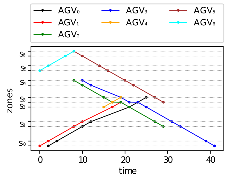
Figure 4: Solution in the form of a space-time diagram, classical ILP solution.

In Tab. 8, the size of ILP is compared with upper limits estimations derived in Section 3.2. We may roughly conclude, referring also to Eqs. (27) (23) (28), that the problem size scale with the square of number of AGVs ($|\mathcal{J}|$) and is linear with the number of zones ($|\mathcal{S}|$).

$|\mathcal{J}|$ / $|\mathcal{S}|$	real ILP			upper limit
	n.o. vars int / bin	n.o. equalities	n.o. inequalities	n.o. vars Eq. (27)	equalities Eq. (23)	inequalities Eq. (28)
2 / 4	16  12/4	4	16	20	16	32
4 / 4	36  20/16	10	34	56	62	124
6 / 7	78  38/40	32	80	189	252	504
7 / 7	118  48/70	55	127	245	343	686
12 / 7	596  102/494	429	766	630	1008	2016
15 / 7	696  118/576	495	883	945	1575	3150

Table 8: Sizes of various AGV problems, in terms of ILP.

References

- Arute et al. (2019) Arute, F., Arya, K., Babbush, R., Bacon, D., Bardin, J.C., Barends, R., Biswas, R., Boixo, S., Brandao, F.G., Buell, D.A., et al., 2019. Quantum supremacy using a programmable superconducting processor. Nature 574, 505–510.
- Brooks (2019) Brooks, M., 2019. Beyond quantum supremacy: the hunt for useful quantum computers. Nature 574, 19–21.
- D-Wave Systems Inc. (2022a) D-Wave Systems Inc., 2022a. Hybrid Solver for Constrained Quadratic Model [WhitePaper]. https://www.dwavesys.com/media/rldh2ghw/14-1055a-a_hybrid_solver_for_constrained_quadratic_models.pdf, visited 2023.08.31.
- D-Wave Systems Inc. (2022b) D-Wave Systems Inc., 2022b. Hybrid Solver for Quadratic Optimization [WhitePaper]. https://www.dwavesys.com/media/soxph512/hybrid-solvers-for-quadratic-optimization.pdf, visited 2023.08.31.
- Domino et al. (2023) Domino, K., Koniorczyk, M., Krawiec, K., Jałowiecki, K., Deffner, S., Gardas, B., 2023. Quantum annealing in the NISQ era: railway conflict management. Entropy 25, 191.
- Evers and Koppers (1996) Evers, J.J., Koppers, S.A., 1996. Automated guided vehicle traffic control at a container terminal. Transportation Research Part A: Policy and Practice 30, 21–34.
- Farhi et al. (2000) Farhi, E., Goldstone, J., Gutmann, S., Sipser, M., 2000. Quantum computation by adiabatic evolution. arXiv preprint quant-ph/0001106 .
- Geitz et al. (2022) Geitz, M., Grozea, C., Steigerwald, W., Stöhr, R., Wolf, A., 2022. Solving the Extended Job Shop Scheduling Problem with AGVs–Classical and Quantum Approaches, in: International Conference on Integration of Constraint Programming, Artificial Intelligence, and Operations Research, Springer. pp. 120–137.
- Gusmeroli and Wiegele (2022) Gusmeroli, N., Wiegele, A., 2022. EXPEDIS: An exact penalty method over discrete sets. Discrete Optimization 44, 100622.
- Haba et al. (2022) Haba, R., Ohzeki, M., Tanaka, K., 2022. Travel time optimization on multi-AGV routing by reverse annealing. arXiv preprint arXiv:2204.11789 .
- Ho (2000) Ho, Y.C., 2000. A dynamic-zone strategy for vehicle-collision prevention and load balancing in an AGV system with a single-loop guide path. Computers in industry 42, 159–176.
- Hozdić (2015) Hozdić, E., 2015. Smart factory for industry 4.0: A review. International Journal of Modern Manufacturing Technologies 7, 28–35.
- Kadowaki and Nishimori (1998) Kadowaki, T., Nishimori, H., 1998. Quantum annealing in the transverse Ising model. Physical Review E 58, 5355.
- Karimi and Ronagh (2017) Karimi, S., Ronagh, P., 2017. A subgradient approach for constrained binary optimization via quantum adiabatic evolution. Quantum Inf Process 16.
- Karimi and Ronagh (2019) Karimi, S., Ronagh, P., 2019. Practical integer-to-binary mapping for quantum annealers. Quantum Information Processing 18, 1–24.
- Kim et al. (1999) Kim, C., Tanchoco, J., Koo, P.H., 1999. AGV dispatching based on workload balancing. International Journal of Production Research 37, 4053–4066.
- Le-Anh (2005) Le-Anh, T., 2005. Intelligent control of vehicle-based internal transport systems. 51.
- Li et al. (2019) Li, G., Li, X., Gao, L., Zeng, B., 2019. Tasks assigning and sequencing of multiple AGVs based on an improved harmony search algorithm. Journal of Ambient Intelligence and Humanized Computing 10, 4533–4546.
- Luo et al. (2018) Luo, Y., Duan, Y., Li, W., Pace, P., Fortino, G., 2018. A novel mobile and hierarchical data transmission architecture for smart factories. IEEE Transactions on Industrial Informatics 14, 3534–3546.
- Pinedo (2012) Pinedo, M.L., 2012. Scheduling. volume 29. Springer.
- Preskill (2012) Preskill, J., 2012. Quantum computing and the entanglement frontier. arXiv:arXiv:1203.5813.
- Preskill (2018) Preskill, J., 2018. Quantum computing in the NISQ era and beyond. Quantum 2, 79.
- Qiu et al. (2002) Qiu, L., Hsu, W.J., Huang, S.Y., Wang, H., 2002. Scheduling and routing algorithms for AGVs: a survey. International Journal of Production Research 40, 745–760.
- Rossit et al. (2019) Rossit, D.A., Tohmé, F., Frutos, M., 2019. Industry 4.0: smart scheduling. International Journal of Production Research 57, 3802–3813.
- Sabuncuoglu and Bayız (2000) Sabuncuoglu, I., Bayız, M., 2000. Analysis of reactive scheduling problems in a job shop environment. European Journal of operational research 126, 567–586.
- Stock and Seliger (2016) Stock, T., Seliger, G., 2016. Opportunities of sustainable manufacturing in industry 4.0. procedia CIRP 40, 536–541.
- Vikstål et al. (2020) Vikstål, P., Grönkvist, M., Svensson, M., Andersson, M., Johansson, G., Ferrini, G., 2020. Applying the Quantum Approximate Optimization Algorithm to the Tail-Assignment Problem. Phys. Rev. Appl. 14, 034009.
- Vivaldini et al. (2015) Vivaldini, K.C., Rocha, L.F., Becker, M., Moreira, A.P., 2015. Comprehensive review of the dispatching, scheduling and routing of AGVs, in: CONTROLO’2014–proceedings of the 11th Portuguese conference on automatic control, Springer. pp. 505–514.
- Zhong et al. (2020) Zhong, M., Yang, Y., Dessouky, Y., Postolache, O., 2020. Multi-AGV scheduling for conflict-free path planning in automated container terminals. Computers & Industrial Engineering 142, 106371.