Doppler confirmation of TESS planet candidate TOI1408.01: grazing transit and likely eccentric orbit

Abstract

We report an independent Doppler confirmation of the TESS planet candidate orbiting an F-type main sequence star TOI-1408 located 140 pc away. We present a set of radial velocities obtained with a high-resolution fiber-optic spectrograph FFOREST mounted at the SAO RAS 6-m telescope (BTA-6). Our self- consistent analysis of these Doppler data and TESS photometry suggests a grazing transit such that the planet obscures its host star by only a portion of the visible disc. Because of this degeneracy, the radius of TOI-1408.01 appears ill-determined with lower limit about $\sim$1 R_Jup, significantly larger than in the current TESS solution. We also derive the planet mass of $1.69\pm 0.20$ $M_{\rm Jup}$ and the orbital period $\sim 4.425$ days, thus making this object a typical hot Jupiter, but with a significant orbital eccentricity of $0.259\pm 0.026$. Our solution may suggest the planet is likely to experience a high tidal eccentricity migration at the stage of intense orbital rounding, or may indicate possible presence of other unseen companions in the system, yet to be detected.

1 Introduction

The first planet orbiting a normal star was discovered in 1995 by Mayor and Queloz (1995) and immediately became a surprise for the world astronomical community, since the existence of a planet with a mass close to that of Jupiter on a 4-day orbit was difficult to explain by existing models at that time. Discovery of the first transit of a hot Jupiter around HD 209458 (Henry et al., 2000; Charbonneau et al., 2000) showed a low density of such planets, which indicates their predominantly hydrogen-helium composition. Since then, hundreds of hot Jupiters have been discovered, but the details of their formation are still unclear (Dawson et al., 2018). According to the most common view, giant planets form outside the system’s icy boundary and then migrate closer to the star (Armitage, 2007).

Migration can be explained by several competing theories including tidal halting; magnetorotational instabilities; planet - disk magnetic interactions; the Kozai mechanism of a distant perturber; planet traps and planet - planet scattering; etc (see Heller (2019) and references in it).

In this paper, we report the discovery of the hot Jupiter TOI-1408.01 in an elongated orbit with an eccentricity of e$\approx$0.26. Compared to some giant planets with huge eccentricities exceeding 0.9, such as HD 80606b (Naef et al., 2001), TOI-1408.01’s eccentricity is quite moderate, but noticeably exceeds the orbital eccentricities of typical hot Jupiters, which are practically zero. It is likely that TOI-1408.01 is in the final stages of rounding its orbit. The following sections discuss the observations, analysis, and results.

2 Observations and data reduction

Observations were carried out with the aid of 6-m Russian Telescope (BTA) from 2021 to 2023 for twenty observation nights under the program EXPLANATION (EXoPLANet And Transient events InvestigatiON, Valyavin et al. (2022a, b)). Observations are currently being made with the fiber-optic high resolution echelle spectrograph FFOREST. Detailed description of the instrument given in Valyavin et al. (2014, 2020). Briefly, the instrument is a fiber-feed high spectral resolution echelle spectrograph with a resolving power R ($\lambda/\Delta\lambda$) beeing in the range from $\sim$30,000 - 35,000 to $\sim$60,000 - 70,000 with further possibility to upgrade it to higher resolution, up to R$\sim$100,000. The portable fiber optic input module is mounted in the prime focus of the 6-m telescope of the Special Astrophysical Observatory of the Russian Academy of Sciences (SAO RAS, Russia). Presently, the instrument has two working fiber channels with equivalent widths of fiber cores of 0.7 $\arcsec$ and 1.4 $\arcsec$. With these cores and binning 2$\times$2 pixels we applied during our observing runs, the instrument provides the resolving power of R$\sim$60,000 and R$\sim$30,000 respectively. An additional calibration channel provides simultaneous observations of spectra from ThAr and Fabry-Perout(in development) calibration sources. It should also be noted that optical camera of the spectrograph is still under construction reducing its efficiency for $\sim$1 stellar magnitude (Valyavin et al., 2020). Nevertheless, the spectrograph is quite effective for planetary observations of stars as faint as 12^m with CCD camera designed by the Advanced Design laboratory of SAO RAS (Ardilanov et al., 2020). The CCD camera’s electronics with the e2v CCD 4k$\times$4k matrix of 15$\times$15 $\mu$m pixel size provide read-out noise of 2-3 electrons.

Table 1: Doppler shift measurements of TOI1408. BJD - barycentric Julian date. Radial velocity (RV) shift values are relative to a template spectrum.

BJD-2450000	RV (m s-1)	BJD-2450000	RV (m $s^{-1}$)
9532.49283	-5604.40 $\pm$ 31.20	9801.34242	-5596.47 $\pm$ 37.46
9536.48208	-5685.88 $\pm$ 21.00	9802.31601	-5582.74 $\pm$ 24.54
9537.22933	-5759.83 $\pm$ 29.69	9834.37490	-5734.37 $\pm$ 30.49
9540.53171	-5524.08 $\pm$ 35.51	9892.26624	-5916.12 $\pm$ 18.51
9624.47869	-5580.01 $\pm$ 09.78	9896.23607	-5886.04 $\pm$ 17.92
9653.55195	-5993.58 $\pm$ 11.80	9899.17260	-5636.53 $\pm$ 39.96
9659.45749	-5743.06 $\pm$ 23.50	9920.19302	-5879.30 $\pm$ 08.55
9662.57867	-5966.79 $\pm$ 66.11	9921.42476	-5719.47 $\pm$ 51.66
9798.36145	-5681.52 $\pm$ 13.89∗	9947.22310	-5734.23 $\pm$ 19.50
9799.44302	-5863.04 $\pm$ 27.33

^∗ In-transit measurement that was removed.

All the spectra were processed with the aid of our own software package DECH (Galazutdinov, 2022) providing all the stages of echelle image/spectra processing, measurements and analysis. Doppler shift measurements were performed with our own code, incorporated into the DECH package. The code based on the cross-correlation algorithm offered by Tonry & Davis (1979). The instrument stability is controlled and corrected by means of simultaneous registration of ThAr spectrum in the adjacent echelle sub-orders observed through an independent optical path (a fiber). Currently FFOREST provides measurements of Doppler shift accuracy limit $\sim$10-20 m s^-1 for stellar spectra, and $\sim$1 m s^-1 for ThAr spectra. The accuracy of radial velocity of some data given in Table 1 is worse due to lower signal-to-noise ratio (SNR) in the corresponding spectra.

2.1 TESS photometry

In the MAST (Mikulski Archive for Space Telescopes) we identified $193$ TESS transit lightcurves of TOI1408. After cutting the range of $\pm 100$ min about each midtransit point, we had $10287$ data points in total. However, different transit lightcurves contained different number of data points, with two clear groups of transits. In the first group there were $<25$ data points per transit, and in the second one there were about $80-90$ data points per transit. Only a few transits appeared between these two groups. Since our software assigns an individual model per each transit, we selected only those transits that had $>80$ data points. There were $96$ such transits, containing $8580$ data points. Thus we preserved $>80\%$ of the total data for our analysis.

2.2 Stellar parameters

Stellar parameters where initially estimated spectroscopically, using the ionization balance method optimized for Solar type stars (Takeda, Ohkubo, & Sadakane, 2002). Calculations were performed with the equivalent widths of $\sim$100 - 120 neutral and $\sim$12 - 15 ionized iron lines measured in our echelle spectra. Derived $T_{\rm eff}$, $\log g$, and $\rm[Fe/H]$ are shown in Table 2. Relatively large uncertainties of these initial values are due to moderate signal-to-noise of available spectra and limited number of measured lines of iron. We then refined stellar parameter with the aid of MIST isochrones (Dotter, 2016) with simultaneous estimation of the star mass $M_{\star}$ and radius $R_{\star}$. The procedure was as follows: for given [Fe/H] and standard A_v = 3.1 we got all isochrone’s points belonging to the main sequence and lying in the uncertainty ranges of initial $T_{\rm eff}$, $\log g$. There are found 53 points with surprisingly low scatter as it is seen in the refined stellar parameters given in Table 2 ($T_{\rm eff}$, $\log g$ marked with MIST).

Also, based on trilinear interpolation of tables by Claret (2017), we derived the limb-darkening coefficients, also shown in the table (for the quadratic limb-darkening law). However, we must notice that there are multiple measurements of $M_{\star}$, $R_{\star}$ in the literature, and they cover rather wide spread of values (we also give them in Table 2 for reference). They are not always consistent with each other, in particular our $R_{\star}$ measurement appears significantly smaller then the one provided by TICv8 (Stassun et al., 2019). However, these data for TOI1408 look incomplete, because they mention zero metallicity, so they might appear not very reliable. GAIA DR3 $R_{\star}$ estimation is based on just the photometry, so it might appear less trustable too.

We rely our further analysis on the $M_{\star}$, $R_{\star}$ derived from the MIST and our complete set of spectrum-derived parameters. However, determining their realistic uncertainties is more complicated, so we must recognize that they can be improved using spectra with higher spectral resolution and SNR.

Table 2: TOI1408 star data

	Ionization Balance		MIST
$T_{\rm eff}$, $\log g$	$6425\pm 170$ K, $4.64\pm 0.30$		$6306\pm 32$ K, $4.35\pm 0.01$
$\rm[Fe/H]$	$7.79\pm 0.12$
Limb darkening	$A$ = $0.2615$ $B$ = $0.2771$
Mass & radius
		MIST-derived∗	GAIA-derived	TICv8
$M_{\star}/M_{\odot}$		$1.332\pm 0.014$		$1.375^{+0.54}_{-0.27}$
$R_{\star}/R_{\odot}$		$1.276\pm 0.015$	$1.5175^{+0.030}_{-0.031}$	$1.485^{+0.12}_{-0.11}$

^∗ Pearson correlation coefficient = 0.87.

3 Analysis and results

3.1 Preliminary

In our preliminary analysis of SAO radial velocities, we revealed an undoubtful periodic signature at the planet orbital period proposed by the TESS team. However, two main issues appeared. First, the observed RV semiamplitude infers the planet minimum mass of $\sim 1.5-2$ $M_{\rm Jup}$, and together with the TESS-provided planet radius of $r\simeq 0.700\pm 0.055$ $R_{\rm Jup}$ this would imply an unrealistic planet density of $\rho\sim 4-6$ $\rho_{\rm Jup}$ (or $5-8$ g cm^-3, like in a rocky planet). Secondly, there were clear hints of an ecentric orbit (moderately nonsinusoidal RV variation) that needed a detailed treatment.

Large estimation of the planet density $\rho$ might indicate either an overvalued planet mass, or an undervalued planet radius. Wrong mass estimation is unlikely, at least not by a factor of a few. But the radius is more suspicious. According to the available TESS solution, TOI1408.01 demonstrates a grazing transit with near-unit impact parameter. Such a configuration implies model degeneracies that could lead to various biases in the fitted parameters, as well as to overly optimistic uncertainties. Therefore, our first task was to verify the planet radius estimation by performing a self-consistent Doppler+photometry fit.

3.2 Models

We include in our analysis the SAO Doppler time series (with one in-transit point removed) and $96$ TESS transits described in Sect. 2.

The RV model included Keplerian planetary variation (with free eccentricity) and possible linear trend (radial acceleration).

Regarding the TESS photometric data, they come in the raw (unwhitened) and whitened version. We used only the unwhitened one, partly because the whitened data should be fit with a more sophisticated transit model transformed by the whitener in the same way, and partly because the likely-biased TESS planet radius might indicate some inaccuracies of the whitener. Unwhitened flux may involve an increased fraction of longer-period variations appearing on the transit timescale as trends, so to handle them we added a cubic polynomial to the model of each transit.

The remaining noise (both in the RV and the photometry) was treated as white with a fittable jitter parameter (Baluev, 2009). We did not use more complicated noise models like the red noise, because the number of data per a single transit (and in the RV curve) appeared too small for that.

The whole analysis was performed using the PlanetPack software (Baluev, 2013, 2018), which is based, eventually, on optimizing the likelihood function of the task. The star mass and radius estimation from Table 2 were incorporated in this analysis in the form of a 2D Gaussian penalty added to the likelihood function (so they basically served as additional input data with 2D uncertainty).

3.3 Results

Contrary to the nominal TESS solution, in our analysis $r$ always appeared ill-fitted. Basically, we can arbitrarily increase $r$, simultaneously increasing the impact parameter, so that the transit curve remains nearly unchanged. This is illustrated in Fig. 1, where we plot the confidence regions in the $(r,R_{\star})$ plane (based on level contours of the likelihood function). The formal best fit corresponds to $r\sim 4$ $R_{\rm Jup}$, but even $r=\infty$ cannot be formally rejected. Nevertheless, based on the $1-3$-sigma domains, we can put a rough lower limit on $r$ about $1-2$ $R_{Jup}$ respectively.

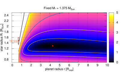
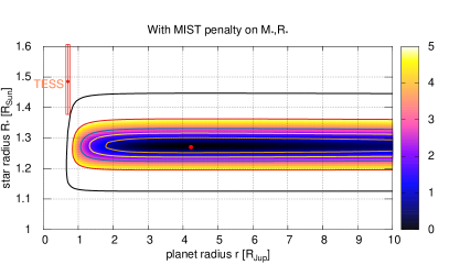
Figure 1: Confidence regions for $(r,R_{\star})$ constructed as level curves of the likelihood function. Five colored curves shown in each panel outline significance levels of $1$-sigma, $2$-sigma, $3$-sigma, $5$-sigma, and $10$-sigma. The colormap shows the same significance (from $0$ to $5$ sigma). The left panel is for $M_{\star}$ fixed at the value from TICv8, but with a priori unconstrained $R_{\star}$, while the right panel involves 2D Gaussian penalty on $M_{\star}$ and $R_{\star}$ derived in this work from the MIST evolutionary tracks.

Normally, transit fits should constrain the star density $\rho_{\star}=M_{\star}R_{\star}^{-3}$, even without any additional astrophysical constraint on $M_{\star}$, $R_{\star}$. But in our case, without the MIST penalty (left panel of Fig. 1), all these parameters remain highly uncertain. Such additional degeneracy comes from the fittable orbital eccentricity. Large eccentricity may affect (i) the transit duration through the planet in-transit orbital speed and (ii) position of the transit on the RV curve. The first effect can also mimic a change in $R_{\star}$, thus making it more uncertain than usually.

Regardless of all these uncertainties, the TESS solution for $(r,R_{\star})$ always lies out of the reasonable significance domain. That is, our analysis does not confirm this solution. In particular, the planet radius has to be significantly larger than the TESS estimation of $0.7$ $R_{\rm Jup}$, and this further confirms our initial guess that $r$ was significantly undervalued by the TESS team.

Table 3: TOI1408: Parameters and best fit values with MIST penalty on $M_{\star}$, $R_{\star}$

Planet			Star
$K$	$178\pm 22$ m/s		$M_{\star}$	$1.331\pm 0.014$ $M_{\odot}$
$P$	$4.4247110\pm 1.6\cdot 10^{-6}$ day		$R_{\star}$	$1.274\pm 0.015$ $R_{\odot}$
$M$	$1.69\pm 0.20$ $M_{\rm Jup}$		$\rho_{\star}$	$0.643\pm 0.018$ $\rho_{\odot}$
$a$	$0.05804\pm 0.00020$ AU
$e$	$0.259\pm 0.026$		Radial acceleration∗
$\omega$	$305.2\pm 5.5$∘		$c_{0}$	$-5739\pm 79$ m/s
$e\cos\omega$	$0.150\pm 0.033$		$c_{1}$	$-25\pm 37$ m/s/yr
$e\sin\omega$	$-0.212\pm 0.013$
$l$	$273.7\pm 4.6^{*}$∘		RV jitter
$i$	$84.801\pm 0.094$∘		$\sigma_{\rm RV}$	$54\pm 11$ m/s
$r/R_{\star}$	$0.1183\pm 0.0014$
$r$	$1.5$ (fixed)$R_{\rm Jup}$

^∗Epoch JD2459000

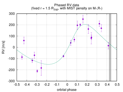
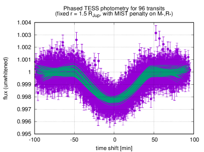
Figure 2: Doppler (left panel) and photometric (right panel) data for TOI1408 and their best fitting models. In the left panel we also mark the position of the transit (as a vertical narrow band). In the right panel, each of $96$ transits has an individual polynomial trend, so we plot a bunch of close curves that differ due to this trend.

Data do not constrain planet radius from the upper side, but it is obvious that $r$ cannot be arbitrarily large, because we deal with a planetary mass object. So to construct at least a reference (not ill-fitted) model, we have to fix $r$ at some a priori reasonable value. For example, the fit for $r=1.5$ $R_{\rm Jup}$ is shown in Table 3. It corresponds to the planet density $\rho=0.50$ $\rho_{\rm Jup}$, a priori rather realistic value for a hot Jupiter. Smaller $r$ would imply larger density, keeping it admissible down to $r\simeq 1$ $R_{\rm Jup}$, while larger $r$ would imply a less likely density below $0.50\rho_{\rm Jup}$. Unfortunately, we cannot say anything more definite about $r$, regardless of so large amount of photometric data. Available data and this reference model are shown together in Fig. 2.

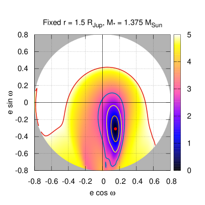
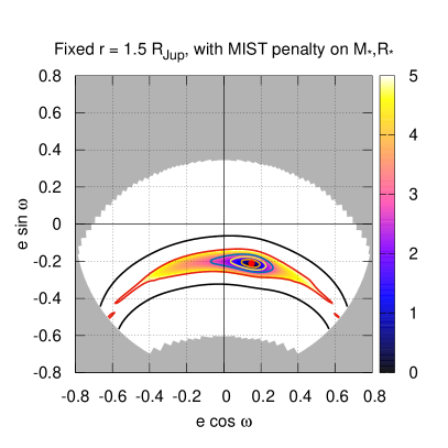
Figure 3: Confidence regions for $(e\cos\omega,e\sin\omega)$. Same notes as in Fig. 1.

As we already noticed, Doppler data reveal important hints of an orbital eccentricity. This is clearly seen from the shape of the RV curve (Fig. 2), and the eccentricity estimation $e$ from Table 3 demonstrate very high formal significance. This eccentricity estimation reveals only a weak dependence on the adopted $r$ (with negative correlation between $r$ and $e$). However, it depends a lot on the adopted $M_{\star}$, $R_{\star}$ penalty. If this penalty is removed, $e$ becomes much more uncertain. This is illustrated in Fig. 3, where we show the 2D confidence plots for the parameters $(e\cos\omega,e\sin\omega)$.

As we noticed above, the MIST penalty may infer overly optimistic uncertainties, so the actuality should likely be somewhere between the left and right panels of Fig. 3. Still, the eccentricity remains significant ($\sim 2.5\sigma$) even in the worst case of no-penalty. Therefore, we believe it is very likely that $e$ is nonzero, although its particular value still need to be refined by more Doppler data. In addition to further Doppler monitoring, it is also necessary to seek for more accurate spectrum (and its parameters of Table 2) in order to refine astrophysical constraint on $M_{\star}$ and $R_{\star}$.

Periodogram did not reveal any extra periodicity after subtracting the planetary signal from the RV data, so presently there is no Doppler hints of more planets in the system.

4 Discussion

In this paper, we explored the transit planetary candidate around the star TOI-1408, discovered by the TESS telescope. Since the period of radial velocity oscillations coincides with the time interval between the centers of transits, we unambiguously confirm its planetary nature. The light curve of the transits has a pronounced V-shape. This indicates the sliding nature of the planetary disk from our spatial perspective, so we cannot estimate the planet’s radius with high accuracy. However, the mass of TOI-1408.01 measured by us, which is $\sim$1.7 M_Jup, indicates a massive gas giant. Such planets are usually comparable to Jupiter in radius (Mordasini et al., 2012) , or even larger, if we take into account the amount of insolation it receives. According to Gaia EDR3 (Gaia Collaboration et al., 2021), the distance to TOI-1408 is 139.6 $\pm$ 0.2 pc, and based on its brightness (G = 9.195^m ), the calculated luminosity of the star exceeds that of the Sun by a factor of 3.26. Assuming zero albedo and effective heat transfer to the night side, we estimate the equilibrium temperature of the planet as $\sim$1550 $K$. The rounding time of the orbit strongly depends on the radius of the planet and the Q_P parameter (Adams & Laughlin, 2006). Assuming Q_P = 10⁶ and the planetary radius in the range of 1.3 - 1.5 R_J, typical for hot Jupiters with high insolation, this time is 0.61 - 1.25 Gyr.

Data availability

The data underlying this article are available in the article and in its online supplementary material.

References

- Adams & Laughlin (2006) Adams F. C., Laughlin G., 2006, ApJ, 649, 1004.
- Ardilanov et al. (2020) Ardilanov V. I., Murzin V. A., Afanasieva I. V. et al. 2020, gbar.conf, 115.
- Armitage (2007) Armitage P. J., 2007, arXiv, astro-ph/0701485.
- Baluev (2009) Baluev R. V., 2009, MNRAS, 393, 969.
- Baluev (2013) Baluev R. V., 2013, A&C, 2, 18.
- Baluev (2018) Baluev R. V., 2018, A&C, 25, 221.
- Charbonneau et al. (2000) Charbonneau D., Brown T. M., Latham D. W., Mayor M., 2000, ApJ, 529, L45
- Claret (2017) Claret A., 2017, A&A, 600, A30.
- Dawson et al. (2018) Dawson R.I., Johnson J.A., 2018, ARA&A 56, 175
- Dotter (2016) Dotter A., 2016, ApJS, 222, 8.
- Gaia Collaboration et al. (2021) Gaia Collaboration, Brown A. G. A., Vallenari A. et al., 2021, A&A, 649, A1.
- Galazutdinov (2022) Galazutdinov G. A., 2022, AstBu, 77, 519.
- Heller (2019) Heller R., 2019, A&A, 628, A42.
- Henry et al. (2000) Henry G. W., Marcy G. W., Butler R. P., Vogt S. S., 2000, ApJ, 529, L41
- Mayor and Queloz (1995) Mayor M.and Queloz D., 1995, Nature, 378, 355
- Mordasini et al. (2012) Mordasini C., Alibert Y., Georgy C. et al. 2012, A&A, 547, A112.
- Naef et al. (2001) Naef D., Latham, D. W., Mayor, M. et al. 2001, A&A, 375, L27
- Stassun et al. (2019) Stassun K. G., Oelkers R. J., Paegert M. et al., 2019, AJ, 158, 138.
- Takeda, Ohkubo, & Sadakane (2002) Takeda Y., Ohkubo M., Sadakane K., 2002, PASJ, 54, 451.
- Tonry & Davis (1979) Tonry J., Davis M., 1979, AJ, 84, 1511.
- Valyavin et al. (2022a) Valyavin G., Beskin G., Valeev A. et al., 2022, AstBu, 77, 495
- Valyavin et al. (2022b) Valyavin G., Beskin G., Valeev A. et al., 2022, Photonics, 9, 950
- Valyavin et al. (2014) Valyavin G. G., Bychkov V. D., Yushkin M.V. et al., 2014, AstBu, 69, 224
- Valyavin et al. (2020) Valyavin G. G., Musaev F. A., Perkov A.V. et al., 2020, AstBu, 75, 191