Sparse 3D Reconstruction via Object-Centric Ray Sampling

Abstract

We propose a novel method for 3D object reconstruction from a sparse set of views captured from a 360-degree calibrated camera rig. We represent the object surface through a hybrid model that uses both an MLP-based neural representation and a triangle mesh. A key contribution in our work is a novel object-centric sampling scheme of the neural representation, where rays are shared among all views. This efficiently concentrates and reduces the number of samples used to update the neural model at each iteration. This sampling scheme relies on the mesh representation to ensure also that samples are well-distributed along its normals. The rendering is then performed efficiently by a differentiable renderer. We demonstrate that this sampling scheme results in a more effective training of the neural representation, does not require the additional supervision of segmentation masks, yields state of the art 3D reconstructions, and works with sparse views on the Google’s Scanned Objects, Tank and Temples and MVMC Car datasets.

	COLMAP*-50	NeRS	RegNeRF	DS	Ours	GT

Figure 1: Left: Sparse view setting of a $360^{\circ}$ camera rig with 8 views. Right: 3D reconstructions with existing SotA methods. Due to the sparsity and wide spacing of the camera views, methods such as NeRS [63] and RegNeRF [38] reconstruct surfaces with visible artifacts. COLMAP^∗ [45, 44] returned a valid mesh only with 50 views (so is used only as a reference). Methods such as DS [15] obtain better reconstructions, but with fewer details than with our approach. Most methods make use of masks to segment the object in each view. In contrast, our method can work without this additional supervision and still obtain accurate 3D reconstructions (compare to the GT).

1 Introduction

The task of reconstructing the 3D surface of an object from multiple calibrated views is a well-established problem with a long history of methods exploring a wide range of 3D representations and optimization methods [11, 12, 10, 51]. Recent approaches have focused their attention on deep learning models [37, 48, 33, 20, 63, 5, 26, 32]. In particular, methods based on neural rendering such as NeRF and its variants [33, 40, 3, 4, 59], have not only shown impressive view interpolation capabilities, but also the ability to output 3D reconstructions as a byproduct of their training.

NeRF’s neural rendering drastically simplifies the generation of images given a new camera pose. It altogether avoids the complex modeling of the light interaction with surfaces in the scene. A neural renderer learns to output the color of a pixel as a weighted average of 3D point samples from the NeRF model. Current methods choose these samples along the ray defined by the given pixel and the camera center (see Figure 2 left). Because each camera view defines a separate pencil of rays, the 3D samples rarely overlap. Thus, each view will provide updates for mostly independent sets of parameters of the NeRF model, which can lead to data overfitting. In practice, overfitting means that views used for training will be rendered correctly, but new camera views will give unrealistic images. Such overfitting is particularly prominent when training a NeRF on only a sparse set of views with a broad object coverage (e.g., see the $360^{\circ}$ camera rig in Figure 1).

In this work, we address overfitting when working with sparse views by proposing an object-centric sampling scheme that is shared across all views (see Figure 2 right and Figure 3). We design the scheme so that all (visible) views can provide an update for the same 3D points on a given sampling ray. To do so, we introduce a hybrid 3D representation, where we simultaneously update a Multi Layer Perceptron (MLP) based implicit surface model (similarly to a NeRF) and an associated triangle mesh. The MLP model defines an implicit 3D representation of the scene, while the mesh is used to define the sampling rays. These rays are located at each mesh vertex and take the direction of the normal to the mesh. Then, the mesh vertex of the current object surface is updated by querying the MLP model at 3D samples on the corresponding ray. We use a similar deep learning model to associate color to the mesh. We then image the triangle mesh in each camera view via a differentiable renderer. Because of our representation, the queried 3D samples can be shared across multiple views and thus avoid the overfitting shown by NeRF models in our settings.

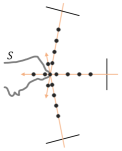
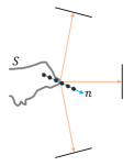
Figure 2: Sampling schemes. Left: NeRF view-centric sampling scheme. Right: Our object-centric sampling scheme. The view-centric sampling scheme uses separate sets of 3D samples for each camera view. This leads to overfitting when views are sparse. Object-centric sampling instead shares the same 3D samples across multiple views.

Notice that a common practice to handle overfitting in NeRF models trained on sparse views is to constrain the 3D reconstruction through object masks. Masks provide a very strong 3D cue. In fact, a (coarse) reconstruction of an object can even be obtained from the masks alone, a technique known as shape from silhouette [23]. We show that our method yields accurate 3D reconstructions even without mask constraints. This confirms experimentally the effectiveness of our sampling scheme in avoiding overfitting.

To summarize, our contributions are

• A novel object-centric sampling scheme that efficiently shares samples across multiple views and avoids overfitting; the robustness of our method is such that it does not need additional constraints, such as 2D object masks;

• A 3D reconstruction method that yields state of the art results with a sparse set of views from a 360-degree camera rig (on the Google’s Scanned Objects [9], Tank and Temples [22] and MVMC Car datasets [63]).

2 Prior Work

Mesh-based methods. With the development of differentiable renderers [19, 50, 5, 17], object reconstruction is now possible through gradient descent (or backpropagation in the context of deep learning). A common approach to predict the shape of an object using differentiable rendering is to use category level image collections [18, 14, 61, 47, 53, 34]. Recently, some methods aim to estimate the shape of an object in a classic multi-view stereo setting and without any prior knowledge of the object category [63, 15, 57, 58, 35]. Several methods also propose different ways to update the surface of the reconstructed object. The methods proposed by Goel et al. [15] and Worchel et al. [57] update the mesh surface by predicting vertex offsets to the template mesh. Zhang et al. [63] use a neural displacement field over a canonical sphere, but restrict the geometry to model only genus-zero topologies. Xu et al. [58], after getting a smooth initial shape via [60], proposes surface-based local MLPs to encode the vertex displacement field for the reconstruction of surface details. Munkberg et al. [35] use a hybrid representation as we do in our method. They learn the signed distance field (SDF) of the reconstructed object. The SDF is defined on samples on a fixed tetrahedral grid and then converted to a surface mesh via deep marching tetrahedra [46]. In contrast, we adapt the samples to the surface of the object as we reconstruct it.

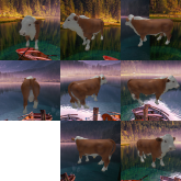
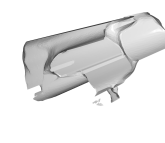
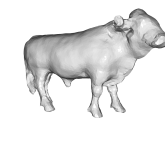
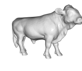
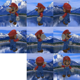
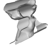
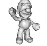
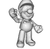
Figure 3: View vs object-centric sampling (see Figure 2). Computational efficiency: The view-centric approach uses $8\times K$ samples per mesh vertex, with $K$ camera views. In contrast, the object-centric approach uses only $8$ samples per vertex regardless of the number of camera views. Object-centric sampling is not only more efficient but also avoids overfitting. For more details, please check Section 3.

Implicit representations for volume rendering. Recently, Neural Radiance Field (NeRF)-based methods have shown great performance in novel view synthesis tasks [33, 64, 54, 2, 25, 49, 30, 43]. However, these methods require a dense number of training views and camera poses to render realistic views. Methods that tackle novel view rendering from a small set of training views usually exploit two directions. The methods in the first group pre-train their models on large scale calibrated multiview datasets of diverse scenes [6, 4, 56, 62, 41, 27, 24]. In our approach, however, we consider training only on a small set of images.

The methods in the second group add an additional regularization term to their optimization cost to handle the limited number of available views. Diet-Nerf [16] incorporates an additional loss that encourages the similarity between the pre-trained CLIP features between the training images and rendered novel views. RegNerf [38] incorporates two additional loss terms: 1) color regularization to avoid color shifts between different views and 2) geometry regularization to enforce smoothness between predicted depths of neighboring pixels. InfoNerf [21] adds a ray entropy loss to minimize the entropy of the volume density along each ray (thus, they encourage the concentration of the volume density on a single location along the ray). This is not suitable for sparse 360-degree camera rigs, where the camera positions lie at the same elevation angle (as in our case) as a ray can be shared by two opposite camera centers. They also add a loss that minimizes the KL-divergence between the normalized density profiles of two neighboring rays. DS-Nerf [8] instead improves the reconstruction quality by adding depth supervision. As they report, its performance is only as good as the estimates of depth obtained by COLMAP [45, 44]. Common to all of the above methods is that they require some sort of additional training (except InforNerf [21]), while our method reconstructs objects without any additional pre-training.

Implicit representations for surface rendering. [52] provides an overview of methods that use implicit representations for either volume or surface rendering. This family of approaches uses a neural SDF or an occupancy field as an implicit surface representation. DVR [37] and IDR [59] are pioneering SDF methods that use only images for training. They both provide a differentiable rendering formulation using implicit gradients. However, both methods require accurate object masks as well as appropriate weight initialization due to the difficulty of propagating gradients. IRON [65] proposes a method to estimate edge derivatives to ease the optimization of neural SDFs. Some of the methods combine implicit surface models with volumetric ones [55, 60, 39] and also implicit surface models with explicit ones [31, 42, 7]. One advantage of the methods that combine implicit surface models with volumetric ones is that they do not require mask supervision and are more stable. However, they heavily depend on a large number of training images. SparseNeuS [28] can work in the sparse view setting, but requires pre-training on a multi-view dataset of multiple scenes. Additionally, it is pretrained only for the narrow view setup, as opposed to the 360-degree one.

3 Sparse 3D Reconstruction

3.1 Problem Formulation

Our goal is to reconstruct the 3D surface of the object depicted in $N$ images $I=\{I_{1},I_{2},\cdots,I_{N}\}$ given their corresponding calibrated camera views $\Pi=\{\pi_{1},\pi_{2},\cdots,\pi_{N}\}$, where $\pi_{i}$ denotes the 3D camera pose and intrinsic camera calibration parameters. We consider the sparse setting, i.e., when $N$ is small (e.g., $8-15$ views). We mostly use camera views distributed uniformly in a $360^{\circ}$ rig (see Figure 1), but our method can also work for the narrow view setup (see the supplementary material for experiments with this setting). We pose the 3D reconstruction task as the problem of finding the 3D surface and texture such that the images $I^{r}=\{I_{1}^{r},\dots,I_{N}^{r}\}$ rendered with the given camera views $\Pi$, best match the corresponding set of captured images $I$.

3.2 3D Representation

We describe the surface of the 3D object via a hybrid model that maintains both an implicit (density-based) and explicit (mesh-based) representation. The two representations serve different purposes. The explicit one is used to efficiently render views of the object and is directly obtained from the implicit representation. The advantage of the implicit representation is that it can smoothly transition through a general family of 3D shapes (e.g., from a sphere to a torus). This is especially useful when the 3D reconstruction is achieved through iterative gradient-based optimization algorithms. Such transition is typically much more difficult to achieve with a lone explicit representation. More specifically, the implicit representation is based on the Implicit Surface Neural Network (ISNN) $F_{\text{shape}}:\mathbb{R}^{3}\rightarrow\mathbb{R}$, that outputs the object density value $\sigma\doteq F_{\text{shape}}(X)$ at a 3D point $X\in\mathbb{R}^{3}$. The explicit representation is obtained by converting the implicit representation in $F_{\text{shape}}$ to a triangle mesh $\mathcal{G}=(\mathcal{V},\mathcal{F})$ consisting of $M$ vertex locations $\mathcal{V}$ and a face list $\mathcal{F}$. A triangle in $\mathcal{F}$ is the triplet of indices of the vertices in $\mathcal{V}$ that form that triangle. The conversion of $F_{\text{shape}}$ to the explicit representation mesh is based on the selection of a finite set of 3D points, which we call samples and discuss in detail in the next section.

3.3 Object-Centric Sampling

In Figure 4, we show a 2D slice of the implicit representation of the cow 3D shape. The implicit representation will have a density $\sigma$ that is close to $1$ at the surface of the object and $0$ elsewhere. In an iterative procedure, we can assume that we already have some existing mesh that is sufficiently close to the current surface of the implicit representation (recall that the implicit representation will be updated through the optimization procedure). To also update the mesh, we use its existing mesh vertices and normals to define segments that are approximately normal to the updated implicit surface and to select samples on the segments in equal number on either side of the surface.

More formally, for each vertex $V_{i}\in\mathcal{V}$, $i=1,\dots,M$, in the current out-of-date mesh, we define a sampling ray $R_{i}$, such that $R_{i}\propto N_{i}$, where $N_{i}$ is the surface normal at the vertex $V_{i}$. Along the ray $R_{i}$ we draw $K$ 3D samples $X_{i,1},\dots,X_{i,K}$ (in Figure 4 we show $K=4$). We define outward and inward point samples by drawing $K$ equally spaced 3D points from the segments $[V_{i},V_{i}+t_{i}^{\text{out}}N_{i}]$ and $[V_{i}-t_{i}^{\text{in}}N_{i},V_{i}]$, where $t_{i}^{\text{in}},t_{i}^{\text{out}}>0$. The range factors $t_{i}^{\text{in}}$ and $t_{i}^{\text{out}}$ are defined independently so that samples on either one of the two segments stay always either inside or outside the mesh, with a maximum possible range. This choice allows to deal with the reconstruction of thin structures of the mesh (e.g., the leg of a horse). For each 3D point we obtain corresponding densities $\sigma_{i,1},\cdots,\sigma_{i,K}$ from the ISNN via $\sigma_{i,j}=F_{\text{shape}}(X_{i,j})$. We then compute normalized weights via the softmax function as $w_{i,j}\propto\exp(\sigma_{i,j})$, such that $\sum_{j=1}^{K}w_{i,j}=1$. Finally, we define the updated mesh vertex $V_{i}$ as the following weighted sum

$$\hat{V}_{i}=\sum_{k=1}^{K}w_{i,k}X_{i,k}.$$ (1)

See Figures 6 and 4 for an illustration of these steps.

Remark. In view-centric methods, such as NeRF, the sampling rays are defined via the camera directions. The view-centric approach presents two drawbacks: Firstly, the number of points grows linearly with the number of cameras. Secondly, when using view-centric (VC) sampling, the surface can only evolve within the subspace determined by the camera poses, resulting in elongated shapes (as observed in Figure 3). This limitation becomes particularly challenging in scenarios with sparse camera views.

Adding Texture. Instead of obtaining color directly from the ISNN as in NeRF models [33, 64, 2, 49, 30], we introduce a separate model, the Texture Neural Network (TNN) $F_{\text{texture}}:\mathbb{R}^{P}\mapsto\mathbb{R}^{3}$, where $P$ is the size of the 3D position embedding. Given the updated 3D vertex location $\hat{V}_{i}$, we compute its positional embedding $\gamma(\hat{V}_{i})$, where $\gamma(\cdot)$ denotes the positional encoding operator, and then obtain the color $C_{i}\doteq F_{\text{texture}}(\gamma(\hat{V}_{i}))$.

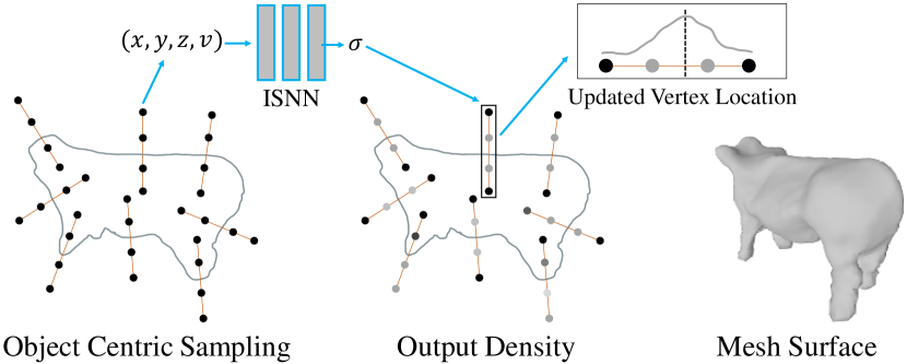
Figure 4: Detailed model representation. We feed the object-centric points to ISNN and obtain a density value. Then, we update the vertex location via eq. (1) using the points sampled along the vertex normal. We repeat this operation for all vertices to get the updated mesh surface.

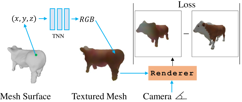
Figure 5: We assign a color to each vertex of the mesh by querying the TNN model at that vertex. Then, we feed the textured mesh and a camera viewpoint as input to a differentiable renderer to synthesize a view of the scene. The reconstruction task is based on minimizing the difference between the synthesized view and a captured image (with the same viewpoint) in both $L_{1}$ and perceptual norms.

Image Rendering. The above procedure yields an updated triangle mesh $\hat{\mathcal{G}}=(\hat{\mathcal{V}},\mathcal{F})$, where $\hat{\mathcal{V}}=\{\hat{V}_{1},\dots,\hat{V}_{M}\}$, with corresponding vertex colors $C=\{C_{1},\dots,C_{M}\}$. We render the image viewed by the $j$-th camera with calibration $\pi_{j}$, $j\in\{1,\dots,N\}$, by feeding $\hat{\mathcal{G}}$ and the vertex colors $C$ to a differentiable renderer [50, 19, 5, 17]. This yields the rendered image $I_{j}^{r}=\mathtt{Renderer}(\hat{\mathcal{G}},C,\pi_{j})$ (see Figure 5).

Reconstruction Loss. $F_{\text{shape}}$ and $F_{\text{texture}}$ are parametrized as Multi Layer Perceptron (MLP) networks (more details of their architectures are in section 4.1). We train their parameters by minimizing the following loss on the images $I$

$$L=L_{\text{images}}(I,I^{r})+L_{\text{perceptual}}(I,I^{r})+\lambda L_{\text{laplacian}}(\hat{\mathcal{G}})$$ (2)

where $L_{\text{images}}(I,I^{r})=\sum_{i=1}^{N}|I_{i}-I_{i}^{r}|_{1}$ is the $L_{1}$ loss between the rendered images and captured images. $L_{\text{perceptual}}$ is the same loss as $L_{\text{images}}$, but where instead of the $L_{1}$ loss we use the perceptual loss [66] and $L_{\text{Laplacian}}$ is the Laplacian loss of the mesh $\hat{\mathcal{G}}$ [36], which we use to regularize the reconstructed 3D vertices $\hat{\mathcal{V}}$ through the parameter $\lambda>0$. We optimize the loss $L$ using the AdamW optimizer [29].

3.4 Technical Details

We employ several ideas to make the optimization robust and accurate.

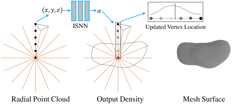
Figure 6: Mesh initialization. The points in the radial point cloud are fed to ISNN to obtain a density value. Then, for each ray we update the vertex location using eq. (1). By repeating this operation for all rays, we obtain the mesh surface.

Mesh Initialization. We use a robust initialization procedure to obtain a first approximate surface mesh. We start from a predefined sphere mesh with radius $\rho$. This sphere defines vertices and triangles of the mesh $\mathcal{G}$. Then, for each vertex $V_{i}\in\mathcal{V}$ we cast a ray $R_{i}$ in the radial direction from the origin of the sphere towards the vertex $V_{i}$ and draw $K$ equally spaced points $X_{i,1},\cdots,X_{i,K}$ along the ray $R_{i}$, such that $|X_{i,K}|_{2}=\rho$ (see Figure 6). These 3D points are never changed throughout this initial model training. The mesh vertices are then computed as in eq. (1). Because each linear combination considers only samples $X_{i,1},\cdots,X_{i,K}$ along a ray, the initial representation $F_{\text{shape}}^{\text{init}}$ can only move the updated vertices radially. Although the reconstructed mesh can model only genus zero objects and only describe a radial structure, it gives us a very reliable initial mesh.

Surface Normals. Surface normals are computed by averaging the normals of the faces within the second order neighbourhood around $V_{i}$.

Re-meshing. Every $100$ iterations during the first $2500$ iterations, and then every $250$ iterations afterwards, we apply a re-meshing step that regularizes and removes self-intersections from the mesh $\mathcal{G}$. This is a separate step that is not part of the optimization of the loss eq. (2) (i.e., there is no backpropagation through these operations). Through re-meshing, the mesh can have genus different from zero and its triangles are adjusted so that they have similar sizes. We use the implementation available in PyMesh - Geometry Processing Library [1]. For more details, see the supplementary material. Notice that the total time for the above calculations during training is almost negligible as we do not apply these operations at every iteration and they are highly optimized.

Inside/Outside 3D Points. For the identification of which 3D samples are inside/outside the 3D surface we use the generalized winding number technique, which is also available in the PyMesh - Geometry Processing Library [1].

Texture Refinement. During training, we observe that the TNN model does not learn to predict sharp textures. Therefore, we run a final phase during which the mesh is kept constant and we fine-tune the TNN separately. Following IDR [59], we feed the vertex location, the vertex normal and the camera viewing direction to the TNN so that it can describe a more general family of reflectances. These quantities are concatenated to $\gamma(\hat{V}_{i})$ and then fed as input to $F_{\text{texture}}$. As described earlier on, in this final phase, we optimize eq. (2) only with respect to the parameters of $F_{\text{texture}}$.

Handling the Background. So far, we have not discussed the presence of a background in the scene and have focused instead entirely on the surface of the object. Technically, unless a mask for each view is provided, there is no explicit distinction between the object and the background. Masks give a strong 3D cue about the reconstructed surface, so much so that they can do most of the heavy-lifting in the 3D reconstruction. Thus, to further demonstrate the strength of our sampling and optimization scheme, we introduce a way to avoid the use of user pre-defined segmentation masks. We extend our model with an approximate background mesh representation. For simplicity, we initialize the background on a fixed mesh (a cuboid) that is sufficiently separated from the volume of camera frustrums’ intersections. When we reconstruct the background, we only optimize the texture assigned to each vertex of the background. Note that we add a separate TNN to estimate the texture of the background and the texture is view-independent at all stages. See also the supplementary material for further details.

Table 1: Reported 3D metrics on the GSO Dataset. *Note that we obtained COLMAP-reconstructed point clouds using 50 views. (**All scores have been multiplied by $10^{4}$). Notice the robustness of our method even when not using the mask constraints.

Method	Mask	CH-L2* $\downarrow$	CH-L1 $\downarrow$	Normal $\uparrow$	F@10 $\uparrow$
NeRS	yes	18.58	0.052	0.54	98.10
RegNeRF	yes	60.19	0.107	0.30	91.44
Munkberg	yes	13.32	0.047	0.56	98.65
DS	yes	13.21	0.042	0.71	98.58
NeuS	no	1217.00	0.495	0.37	32.40
NeuS	yes	13.85	0.049	0.70	98.79
COLMAP*	yes	34.35	0.049	-	99.11
Our wo/BCG	yes	8.69	0.034	0.75	99.24
Our w/BCG	no	11.08	0.038	0.75	98.85

Table 2: GSO Dataset: Quantitative evaluation of generated views on the test set. Notice the robustness of our method even when not using the mask constraints.

Method	Mask	PSNR $\uparrow$	MSE $\downarrow$	SSIM $\uparrow$	LPIPS $\downarrow$
NeRS	yes	20.108	0.0185	0.874	0.126
RegNeRF	yes	20.217	0.013	0.882	0.143
Munkberg et al.	yes	26.838	0.002	0.955	0.067
DS	yes	24.649	0.004	0.944	0.081
Our wo/BCG	yes	29.029	0.001	0.967	0.028
Our w/BCG	no	27.370	0.002	0.964	0.038

4 Experiments

In this section, we present implementation details and results obtained on the standard datasets. For more comprehensive ablation studies as well as for more visual results, we refer to the supplementary material.

4.1 Implementation Details

We parameterize $F_{\text{shape}}^{\text{init}}$, $F_{\text{shape}}$ and $F_{\text{texture}}$ as MLPs with 5, 5, and 3 layers respectively and a hidden dimension of 256 for all. The initialization mesh uses 2500 vertices, while the mesh for the object reconstruction uses a maximum of 10K vertices. For the background mesh we use a vertex resolution of 10K. When training the texture network TNN in the final step, we upsample the mesh resolution to 250K vertices. The scale $t_{in}$ and $t_{out}$ for the detailed model reconstruction are both set to $0.15$. The number of samples along the rays for $F_{\text{shape}}^{\text{init}}$ and $F_{\text{shape}}$ is $16$ and $8$ respectively. The learning rate for the training of the initialization, shape, and texture models is $10^{-5}$, $5\times 10^{-5}$, and $10^{-3}$. The Laplacian regularization may change across datasets. For objects with non-Lambertian surfaces, e.g., specular surfaces, we use a higher Laplacian regularization, as in this case the $F_{\text{shape}}$ network can overfit and generate spiky surfaces due to the lack of multiview consistency across the views. We will release the code of all components of our work to facilitate further research and allow others to reproduce our results.

Table 3: MVMC Car Dataset: Quantitative evaluation of generated views on the test set. Our wo/BCG* and Our w/BCG are trained with the same pre-processing as in NeRS.

Method	Mask	PSNR $\uparrow$	MSE $\downarrow$	SSIM $\uparrow$	LPIPS $\downarrow$
NeRS	yes	18.381	0.015	0.852	0.080
RegNeRF	yes	15.776	0.028	0.751	0.259
Munkberg et al.	yes	15.145	0.031	0.761	0.239
DS	yes	18.608	0.015	0.835	0.139
Our w/BCG*	no	18.301	0.015	0.855	0.132
Our wo/BCG*	yes	20.030	0.010	0.867	0.095
Our w/BCG	no	18.450	0.014	0.865	0.142
Our wo/BCG	yes	21.563	0.007	0.883	0.091

4.2 Datasets

Google’s Scanned Objects (GSO) [9]. We test our algorithm on 14 different objects. For training, we use 8 views, and for validation 100 views. Camera poses are uniformly spread out around the object where the elevation angle is uniformly sampled in $[0^{\circ},15^{\circ}]$. The background image is generated by warping a panorama image onto a sphere.
MVMC Car dataset [63]. We run our algorithm on 5 different cars from the MVMC dataset. We use the optimized camera poses provided in the dataset. Although they are optimized, we find that some of them are not correct. Thus, we eliminated those views for both training and testing. We follow a leave-one-out cross-validation setup, where we leave one view for validation and the rest is used for training. We repeat this 5 times for each car. Note that this dataset is more challenging than the GSO Dataset [9] as the camera locations are not spread out uniformly around the object. Most of the views are placed mainly on two opposite sides of the cars. Furthermore, the surface of cars is not-Lambertian, and there are many light sources present in the scene too.

Tank and Temple dataset [22]. We evaluate our method on images from 2 objects, Truck and Ignatius. We use 15 images for training and the rest as the test set. We obtain the image masks of each object by rendering its corresponding laser-scanned ground-truth 3D point cloud. The camera poses are computed via COLMAP’s SfM pipeline [44].

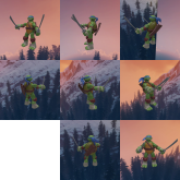
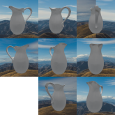
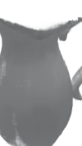
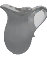
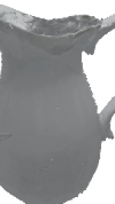
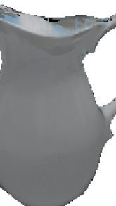
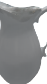
Input Images	RegNeRF	NeRS	Munkberg et al. [35]	DS	our w/BCG*	our wo/BCG	GT

Figure 7: Qualitative Results on the GSO Dataset. Note that in our w/BCG* column we remove the background rendering in the w/BCG column to simplify the visual comparisons.

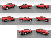
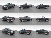
Input	RegNeRF	NeRS*	Munkberg et al. [35]	DS	our w/BCG*	our wo/BCG	GT

Figure 8: Qualitative Results on the MVMC Car dataset. NeRS*: the original NeRS implementation crops the images before training and thus changes their aspect ratio during training. Thus, the rendered images have an aspect ratio of 1, while the original ones do not. For more information, see section 4.3. Note that we remove the background rendering in the w/BCG* column to simplify the visual comparisons.

4.3 Evaluation

Metrics. For the datasets with a 3D ground truth, we compare the reconstructed meshes with the ground-truth meshes or point clouds. More specifically, we report the L2-Chamfer and L1-Chamfer distances, normal consistency, and F1 score, following [13]. We also report texture metrics to evaluate the quality of the texture on unseen views. More specifically, we employ Mean-Square Error (MSE), Peak Signal-to-Noise Ratio (PSNR), and Structural Similarity Index Measure (SSIM), and Learned Perceptual Image Patch Similarity (LPIPS) [66].
Baselines. We compare our method with the following methods: (1) RegNerf [38], a volume rendering method, (2) Munkberg et al. [35], a hybrid-based method, (3) DS [15], a mesh-based method, (4) COLMAP [45, 44], a multi-view stereo method, (5) NeUS [55], neural surface reconstruction method, and (6) NeRS [63] a neural reflectance surface method. Further details about these baseline methods can be found in the supplementary material.

RegNeRF	NeRS	Munkberg et al.	DS	NeuS w/BCG	NeuS wo/BCG	Our w/BCG	Our wo/BCG	GT

Figure 9: Reconstructed meshes for the COW object in the GSO Dataset.

Table 4: Tank and Temples Dataset: Quantitative evaluation of generated views on the test set.

Scene	Method	Mask	PSNR $\uparrow$	MSE $\downarrow$	SSIM $\uparrow$	LPIPS $\downarrow$
Truck	RegNeRF	yes	18.078	0.018	0.657	0.254
	Munkberg et al.	yes	18.398	0.018	0.673	0.245
	Our wo/BCG	yes	18.315	0.017	0.701	0.252
	Our w/BCG	no	13.168	0.0508	0.666	0.343
Ignatius	RegNeRF	yes	21.123	0.105	0.866	0.108
	Munkberg et al.	yes	22.720	0.007	0.873	0.073
	Our wo/BCG	yes	23.022	0.007	0.896	0.080
	Our w/BCG	no	17.845	0.021	0.875	0.153

Table 5: Tank and Temples Dataset: 3D metrics. *Note that we obtained the COLMAP*-reconstructed point clouds using 50 views.

Scene	Method	Mask	Chamfer-L2 $\downarrow$	Chamfer-L1 $\downarrow$	F@$10$ $\uparrow$
Truck	RegNeRF-clean	yes	0.059	0.342	42.56
	Munkberg et al.	yes	0.072	0.355	50.11
	DS	yes	0.110	0.479	31.73
	COLMAP*	yes	0.056	0.298	57.74
	NeuS	no	3.342	2.417	6.50
	NeuS	yes	0.629	1.253	11.93
	Our wo/BCG	yes	0.094	0.406	48.14
	Our w/BCG	no	0.225	0.613	45.78
Ignatius	RegNeRF-clean	yes	0.106	0.423	43.45
	Munkberg et al.	yes	0.022	0.189	81.75
	DS	yes	0.024	0.207	77.68
	COLMAP*	yes	0.013	0.166	86.90
	NeuS	no	0.155	0.572	31.95
	NeuS	yes	0.061	0.3878	37.72
	Our wo/BCG	yes	0.018	0.147	87.12
	Our w/BCG	no	0.139	0.480	55.32

4.4 Results

We run our algorithm under two settings: with background (w/BCG) and by removing the background (wo/BCG), the latter of which is akin to using a mask. We present both qualitative (Figure 7 and Figure 9) and quantitative (Table 1 and Table 2) result on the GSO dataset. We observe that our proposed method for both w/BCG and wo/BCG is able to recover the original shape with high accuracy. DS, Munkberg et al. [35] and NeuS (with mask supervision) show the closest performance to ours. We observe that NeuS without mask supervision struggles to accurately reconstruct the original shape for seven out of the fourteen objects. NeRS is also able to recover the shape, but cannot recover genus 1 objects. RegNeRF shows blur artifacts as a result of the inherent ambiguity of sparse input data and also may miss some parts of the original object, e.g., the leg of the cow object. RegNeRF does not always recover the thin parts of the object, e.g., legs of the horse, and thus the reconstructed geometry is not fully accurate. When we run COLMAP with 8 views we find that for most objects the reconstructed point cloud is mostly empty and the object is not recognizable (see also the supplementary material for visual results). This is not surprising since we have only 8 views covering 360-degrees of the object. Furthermore, in this setting, any surface is visible at most from 3 views and the objects does not have a rich texture. Because of this reason, we run COLMAP with 50 views and present the results in all tables just for reference.

In Figure 8 and Table 3 we present qualitative and quantitative results for car objects on MVMC Car dataset. We qualitatively observe that our method wo/BCG shows better view renderings than other methods. Our method fails to recover the texture around transparent surfaces, e.g., the car window. The model in the w/BCG case is able to recover the main shape of the car, but it misses some parts, e.g., the tires of the car that are attached to the ground due to overlaps with the background mesh. Additionally, the tires contain poor texture, e.g., mostly they are black, so this can be easily captured by the background texture network and thus introduce an ambiguity in the reconstruction. We note that the performance for NeRS is consistent across different cars. This is not surprising as they use the mask and their initial template is also car-like. We do not run COLMAP on this dataset as the dataset has a limited number of views. DS has weaker performance on this dataset compared to the GSO. The main reason for poor texture quality is that texture is obtained by 3D back-projections of the mesh to the input views. Thus, incorrect geometry leads to poor texture quality. We observe that the quality of the reconstructions from RegNeRF and Munkberg et al. [35] lack realism. There are two main reasons for this. Firstly, the camera locations are not uniformly spread out around the object. Most of them are located on two sides of the cars. In this case, the methods struggle to recover the original shape. Secondly, because of the many light sources present in the scene and non-Lambertian surfaces, the multi-view consistency across the views is not satisfied. As can be observed, our method is more robust to the above issues. The main reason for that is that during the training of ISNN, the output color of TNN does not depend on the camera view and thus it is less prone to overfitting.

In Table 5 and Table 4 we present quantitative results for two objects in the Tank and Temple datasets. Note that the performance of all methods is drastically decreased especially in the recovered 3D shape compared to the GSO dataset. This is expected as the ground-truth point clouds are hollow (without the bottom), e.g. Truck, and the reported numbers only approximate the quality of the shape. Our wo/BCG has a higher Chamfer distance compared to the others although it looks visually better. This is because the corresponding ground-truth shape does not only include the target object, but also some other components from the background, as, e.g., in the Truck scene. For visual results and more details, see the supplementary material.

5 Conclusion

We have introduced a novel multi-view stereo method that works with sparse views from a 360 rig. The method can handle this extreme setting by using a novel object-centric sampling scheme and a corresponding hybrid surface representation. The sampling scheme allows to concentrate the updates due to multiple camera views to the same components of the surface representation and to structure the updates so that they result in useful surface changes (along its normals, rather than its tangent space). We have demonstrated the robustness of this method by working without the common mask supervision constraint, by using datasets with diverse 3D objects (GSO Dataset), on scenes with complex illumination sources and with non-Lambertian surfaces (MVMC Car).

References

- [1] Pymesh — geometry processing library for python. https://pymesh.readthedocs.io/en/latest/index.html. Accessed: 2023-03-08.
- Barron et al. [2021] Jonathan T. Barron, Ben Mildenhall, Matthew Tancik, Peter Hedman, Ricardo Martin-Brualla, and Pratul P. Srinivasan. Mip-nerf: A multiscale representation for anti-aliasing neural radiance fields. ICVV, 2021.
- Barron et al. [2022] Jonathan T. Barron, Ben Mildenhall, Dor Verbin, Pratul P. Srinivasan, and Peter Hedman. Mip-nerf 360: Unbounded anti-aliased neural radiance fields. CVPR, 2022.
- Chen et al. [2021] Anpei Chen, Zexiang Xu, Fuqiang Zhao, Xiaoshuai Zhang, Fanbo Xiang, Jingyi Yu, and Hao Su. Mvsnerf: Fast generalizable radiance field reconstruction from multi-view stereo. In ICCV, 2021.
- Chen et al. [2019] Wenzheng Chen, Huan Ling, Jun Gao, Edward Smith, Jaakko Lehtinen, Alec Jacobson, and Sanja Fidler. Learning to predict 3d objects with an interpolation-based differentiable renderer. In Advances in Neural Information Processing Systems, 2019.
- Chibane et al. [2021] Julian Chibane, Aayush Bansal, Verica Lazova, and Gerard Pons-Moll. Stereo radiance fields (srf): Learning view synthesis from sparse views of novel scenes. In CVPR, 2021.
- Chong Bao and Bangbang Yang et al. [2022] Chong Bao and Bangbang Yang, Zeng Junyi, Bao Hujun, Zhang Yinda, Cui Zhaopeng, and Zhang Guofeng. Neumesh: Learning disentangled neural mesh-based implicit field for geometry and texture editing. In ECCV, 2022.
- Deng et al. [2022] Kangle Deng, Andrew Liu, Jun-Yan Zhu, and Deva Ramanan. Depth-supervised NeRF: Fewer views and faster training for free. In CVPR, 2022.
- Downs et al. [2022] Laura Downs, Anthony Francis, Nate Koenig, Brandon Kinman, Ryan Hickman, Krista Reymann, Thomas B. McHugh, and Vincent Vanhoucke. Google scanned objects: A high-quality dataset of 3d scanned household items. In International Conference on Robotics and Automation, 2022.
- Forsyth and Ponce [2002] David A Forsyth and Jean Ponce. Computer vision: a modern approach. Prentice Hall Professional Technical Reference, 2002.
- Furukawa and Ponce [2010] Yasutaka Furukawa and Jean Ponce. Accurate, dense, and robust multiview stereopsis. PAMI, 2010.
- Furukawa et al. [2015] Yasutaka Furukawa, Carlos Hernández, et al. Multi-view stereo: A tutorial. Foundations and Trends® in Computer Graphics and Vision, 2015.
- Georgia Gkioxari [2019] Justin Johnson Georgia Gkioxari, Jitendra Malik. Mesh r-cnn. In ICCV, 2019.
- Goel et al. [2020] Shubham Goel, Angjoo Kanazawa, and Jitendra Malik. Shape and viewpoints without keypoints. In ECCV, 2020.
- Goel et al. [2022] Shubham Goel, Georgia Gkioxari, and Jitendra Malik. Differentiable stereopsis: Meshes from multiple views using differentiable rendering. In CVPR, 2022.
- Jain et al. [2021] Ajay Jain, Matthew Tancik, and Pieter Abbeel. Putting nerf on a diet: Semantically consistent few-shot view synthesis. In ICCV, 2021.
- Johnson et al. [2020] Justin Johnson, Nikhila Ravi, Jeremy Reizenstein, David Novotny, Shubham Tulsiani, Christoph Lassner, and Steve Branson. Accelerating 3d deep learning with pytorch3d. In SIGGRAPH Asia 2020 Courses, 2020.
- Kanazawa et al. [2018] Angjoo Kanazawa, Shubham Tulsiani, Alexei A. Efros, and Jitendra Malik. Learning category-specific mesh reconstruction from image collections. In ECCV, 2018.
- Kato et al. [2018] Hiroharu Kato, Yoshitaka Ushiku, and Tatsuya Harada. Neural 3d mesh renderer. In CVPR, 2018.
- Khot et al. [2019] Tejas Khot, Shubham Agrawal, Shubham Tulsiani, Christoph Mertz, Simon Lucey, and Martial Hebert. Learning unsupervised multi-view stereopsis via robust photometric consistency. In CVPR, 2019.
- Kim et al. [2022] Mijeong Kim, Seonguk Seo, and Bohyung Han. Infonerf: Ray entropy minimization for few-shot neural volume rendering. In CVPR, 2022.
- Knapitsch et al. [2017] Arno Knapitsch, Jaesik Park, Qian-Yi Zhou, and Vladlen Koltun. Tanks and temples: Benchmarking large-scale scene reconstruction. ACM Trans. Graph., 2017.
- Laurentini [1994] Aldo Laurentini. The visual hull concept for silhouette-based image understanding. PAMI, 1994.
- Li et al. [2021] Jiaxin Li, Zijian Feng, Qi She, Henghui Ding, Changhu Wang, and Gim Hee Lee. Mine: Towards continuous depth mpi with nerf for novel view synthesis. In ICCV, 2021.
- Lin et al. [2021] Chen-Hsuan Lin, Wei-Chiu Ma, Antonio Torralba, and Simon Lucey. Barf: Bundle-adjusting neural radiance fields. In ICCV, 2021.
- Liu et al. [2020] Lingjie Liu, Jiatao Gu, Kyaw Zaw Lin, Tat-Seng Chua, and Christian Theobalt. Neural sparse voxel fields. In NeurIPS, 2020.
- Liu et al. [2022] Yuan Liu, Sida Peng, Lingjie Liu, Qianqian Wang, Peng Wang, Christian Theobalt, Xiaowei Zhou, and Wenping Wang. Neural rays for occlusion-aware image-based rendering. In CVPR, 2022.
- Long et al. [2022] Xiaoxiao Long, Cheng Lin, Peng Wang, Taku Komura, and Wenping Wang. Sparseneus: Fast generalizable neural surface reconstruction from sparse views. ECCV, 2022.
- Loshchilov and Hutter [2019] Ilya Loshchilov and Frank Hutter. Decoupled weight decay regularization. In ICLR, 2019.
- Martin-Brualla et al. [2021] Ricardo Martin-Brualla, Noha Radwan, Mehdi S. M. Sajjadi, Jonathan T. Barron, Alexey Dosovitskiy, and Daniel Duckworth. NeRF in the Wild: Neural Radiance Fields for Unconstrained Photo Collections. In CVPR, 2021.
- Mehta et al. [2022] Ishit Mehta, Manmohan Chandraker, and Ravi Ramamoorthi. A level set theory for neural implicit evolution under explicit flows. In ECCV, 2022.
- Mildenhall et al. [2019] Ben Mildenhall, Pratul P. Srinivasan, Rodrigo Ortiz-Cayon, Nima Khademi Kalantari, Ravi Ramamoorthi, Ren Ng, and Abhishek Kar. Local light field fusion: Practical view synthesis with prescriptive sampling guidelines. ACM Trans. Graph., 2019.
- Mildenhall et al. [2020] Ben Mildenhall, Pratul P. Srinivasan, Matthew Tancik, Jonathan T. Barron, Ravi Ramamoorthi, and Ren Ng. Nerf: Representing scenes as neural radiance fields for view synthesis. In ECCV, 2020.
- Monnier et al. [2022] Tom Monnier, Matthew Fisher, Alexei A. Efros, and Mathdieu Aubry. Share With Thy Neighbors: Single-View Reconstruction by Cross-Instance Consistency. In ECCV, 2022.
- Munkberg et al. [2022] Jacob Munkberg, Jon Hasselgren, Tianchang Shen, Jun Gao, Wenzheng Chen, Alex Evans, Thomas Müller, and Sanja Fidler. Extracting Triangular 3D Models, Materials, and Lighting From Images. In CVPR, 2022.
- Nealen et al. [2006] Andrew Nealen, Takeo Igarashi, Olga Sorkine, and Marc Alexa. Laplacian mesh optimization. In International Conference on Computer Graphics and Interactive Techniques in Australasia and Southeast Asia, 2006.
- Niemeyer et al. [2020] Michael Niemeyer, Lars Mescheder, Michael Oechsle, and Andreas Geiger. Differentiable volumetric rendering: Learning implicit 3d representations without 3d supervision. In CVPR, 2020.
- Niemeyer et al. [2022] Michael Niemeyer, Jonathan T. Barron, Ben Mildenhall, Mehdi S. M. Sajjadi, Andreas Geiger, and Noha Radwan. Regnerf: Regularizing neural radiance fields for view synthesis from sparse inputs. In CVPR, 2022.
- Oechsle et al. [2021] Michael Oechsle, Songyou Peng, and Andreas Geiger. Unisurf: Unifying neural implicit surfaces and radiance fields for multi-view reconstruction. In ICCV, 2021.
- Pan et al. [2022] Xuran Pan, Zihang Lai, Shiji Song, and Gao Huang. Activenerf: Learning where to see with uncertainty estimation. In ECCV, 2022.
- Rematas et al. [2021] Konstantinos Rematas, Ricardo Martin-Brualla, and Vittorio Ferrari. Sharf: Shape-conditioned radiance fields from a single view. In ICML, 2021.
- Remelli et al. [2020] Edoardo Remelli, Artem Lukoianov, Stephan Richter, Benoit Guillard, Timur Bagautdinov, Pierre Baque, and Pascal Fua. Meshsdf: Differentiable iso-surface extraction. In NeurIPS, 2020.
- Sara Fridovich-Keil and Alex Yu et al. [2022] Sara Fridovich-Keil and Alex Yu, Matthew Tancik, Qinhong Chen, Benjamin Recht, and Angjoo Kanazawa. Plenoxels: Radiance fields without neural networks. In CVPR, 2022.
- Schonberger and Frahm [2016] Johannes L. Schonberger and Jan-Michael Frahm. Structure-from-motion revisited. In CVPR, 2016.
- Schönberger et al. [2016] Johannes Lutz Schönberger, Enliang Zheng, Marc Pollefeys, and Jan-Michael Frahm. Pixelwise view selection for unstructured multi-view stereo. In ECCV, 2016.
- Shen et al. [2021] Tianchang Shen, Jun Gao, Kangxue Yin, Ming-Yu Liu, and Sanja Fidler. Deep marching tetrahedra: a hybrid representation for high-resolution 3d shape synthesis. In NeurIPS, 2021.
- Simoni et al. [2021] Alessandro Simoni, Stefano Pini, Roberto Vezzani, and Rita Cucchiara. Multi-category mesh reconstruction from image collections. In 3DV, 2021.
- Sitzmann et al. [2019] Vincent Sitzmann, Michael Zollhöfer, and Gordon Wetzstein. Scene representation networks: Continuous 3d-structure-aware neural scene representations. In NeurIPS, 2019.
- Sitzmann et al. [2021] Vincent Sitzmann, Semon Rezchikov, William T. Freeman, Joshua B. Tenenbaum, and Fredo Durand. Light field networks: Neural scene representations with single-evaluation rendering. In NeurIPS, 2021.
- Szabó et al. [2019] Attila Szabó, Givi Meishvili, and Paolo Favaro. Unsupervised generative 3d shape learning from natural images. arXiv:1910.00287, 2019.
- Szeliski [2022] Richard Szeliski. Computer vision: algorithms and applications. Springer Nature, 2022.
- Tewari et al. [2021] Ayush Tewari, Justus Thies, Ben Mildenhall, Pratul Srinivasan, Edgar Tretschk, Yifan Wang, Christoph Lassner, Vincent Sitzmann, Ricardo Martin-Brualla, Stephen Lombardi, Tomas Simon, Christian Theobalt, Matthias Niessner, Jonathan T. Barron, Gordon Wetzstein, Michael Zollhoefer, and Vladislav Golyanik. Advances in neural rendering. arXiv:2111.05849, 2021.
- Tulsiani et al. [2020] Shubham Tulsiani, Nilesh Kulkarni, and Abhinav Gupta. Implicit mesh reconstruction from unannotated image collections. arXiv:2007.08504, 2020.
- Verbin et al. [2022] Dor Verbin, Peter Hedman, Ben Mildenhall, Todd Zickler, Jonathan T. Barron, and Pratul P. Srinivasan. Ref-NeRF: Structured view-dependent appearance for neural radiance fields. In CVPR, 2022.
- Wang et al. [2021a] Peng Wang, Lingjie Liu, Yuan Liu, Christian Theobalt, Taku Komura, and Wenping Wang. Neus: Learning neural implicit surfaces by volume rendering for multi-view reconstruction. In NeurIPS, 2021a.
- Wang et al. [2021b] Qianqian Wang, Zhicheng Wang, Kyle Genova, Pratul Srinivasan, Howard Zhou, Jonathan T. Barron, Ricardo Martin-Brualla, Noah Snavely, and Thomas Funkhouser. Ibrnet: Learning multi-view image-based rendering. In CVPR, 2021b.
- Worchel et al. [2022] Markus Worchel, Rodrigo Diaz, Weiwen Hu, Oliver Schreer, Ingo Feldmann, and Peter Eisert. Multi-view mesh reconstruction with neural deferred shading. In CVPR, 2022.
- Xu et al. [2023] Jiamin Xu, Zihan Zhu, Hujun Bao, and Weiwei Xu. A hybrid mesh-neural representation for 3d transparent object reconstruction. arXiv:2203.12613, 2023.
- Yariv et al. [2020] Lior Yariv, Yoni Kasten, Dror Moran, Meirav Galun, Matan Atzmon, Basri Ronen, and Yaron Lipman. Multiview neural surface reconstruction by disentangling geometry and appearance. NeurIPS, 2020.
- Yariv et al. [2021] Lior Yariv, Jiatao Gu, Yoni Kasten, and Yaron Lipman. Volume rendering of neural implicit surfaces. In NeurIPS, 2021.
- Ye et al. [2021] Yufei Ye, Shubham Tulsiani, and Abhinav Gupta. Shelf-supervised mesh prediction in the wild. In CVPR, 2021.
- Yu et al. [2021] Alex Yu, Vickie Ye, Matthew Tancik, and Angjoo Kanazawa. pixelNeRF: Neural radiance fields from one or few images. In CVPR, 2021.
- Zhang et al. [2021] Jason Y. Zhang, Gengshan Yang, Shubham Tulsiani, and Deva Ramanan. NeRS: Neural reflectance surfaces for sparse-view 3d reconstruction in the wild. In NeurIPS, 2021.
- Zhang et al. [2020] Kai Zhang, Gernot Riegler, Noah Snavely, and Vladlen Koltun. Nerf++: Analyzing and improving neural radiance fields. arXiv:2010.07492, 2020.
- Zhang et al. [2022] Kai Zhang, Fujun Luan, Zhengqi Li, and Noah Snavely. Iron: Inverse rendering by optimizing neural sdfs and materials from photometric images. In CVPR, 2022.
- Zhang et al. [2018] Richard Zhang, Phillip Isola, Alexei A. Efros, Eli Shechtman, and Oliver Wang. The unreasonable effectiveness of deep features as a perceptual metric. In CVPR, 2018.