T-SaS: Toward Shift-aware Dynamic Adaptation for Streaming Data

Abstract.

In many real-world scenarios, distribution shifts exist in the streaming data across time steps. Many complex sequential data can be effectively divided into distinct regimes that exhibit persistent dynamics. Discovering the shifted behaviors and the evolving patterns underlying the streaming data are important to understand the dynamic system. Existing methods typically train one robust model to work for the evolving data of distinct distributions or sequentially adapt the model utilizing explicitly given regime boundaries. However, there are two challenges: (1) shifts in data streams could happen drastically and abruptly without precursors. Boundaries of distribution shifts are usually unavailable, and (2) training a shared model for all domains could fail to capture varying patterns. This paper aims to solve the problem of sequential data modeling in the presence of sudden distribution shifts that occur without any precursors. Specifically, we design a Bayesian framework, dubbed as T-SaS, with a discrete distribution-modeling variable to capture abrupt shifts of data. Then, we design a model that enable adaptation with dynamic network selection conditioned on that discrete variable. The proposed method learns specific model parameters for each distribution by learning which neurons should be activated in the full network. A dynamic masking strategy is adopted here to support inter-distribution transfer through the overlapping of a set of sparse networks. Extensive experiments show that our proposed method is superior in both accurately detecting shift boundaries to get segments of varying distributions and effectively adapting to downstream forecast or classification tasks.

1. Introduction

Deploying machine learning models (Ren et al., 2017; Xu et al., 2018; Zhao et al., 2020, 2023a) in real-world systems often presents the challenge of distribution shift. This occurs when the statistical characteristics of newly incoming data differ from those observed by the model in a dynamically changing environment (Wang and Deng, 2018; De Lange et al., 2021; Ren et al., 2018; Zhao et al., 2022c; Ren et al., 2022b). Generally, the shift can happen without any precursor, be unknown to users, cause dramatic personal injury for systems like self-driving (Liu et al., 2020), robotics (Zhang et al., 2021; Zhao et al., 2023c), sleep tracking (Wilson and Cook, 2020) and irreparable economic damage on financial trading algorithms (Wilson and Cook, 2020; Ren et al., 2021a; Wang et al., 2022; Zhao et al., 2022a). At any moment, the model is expected to 1) provide early warnings when the data distribution changes and 2) make accurate predictions by adapting to new data. Several approaches have been proposed to develop adaptive models for sequential data in dynamic environments, e.g., transfer learning (Wang and Deng, 2018; Wilson and Cook, 2020; Ren et al., 2022a; Zhao et al., 2022b), continual learning (Nguyen et al., 2017; Shen et al., 2023). However, they are unable to deal with sudden or irregular shifts due to parameter-sharing strategies, which limits their model capacity. Besides, these algorithms mainly assume that the data stream is explicitly divided into different regimes (Wang and Deng, 2018) (tasks or domains) according to given change points. In the real world, changes often occur without precursors and explicit temporal segments are unavailable.

Addressing these challenges, we propose an incremental model selection approach in the form of a dynamic network to handle sequentially shifting data. In this paper, we introduce T-SaS, a novel Bayesian-based approach that combines dynamic network selection with a shift points estimation scheme for sequentially evolving data (Ren et al., 2021b). This approach enables the modeling of distinct distributions by evolving the network structure (Zhao et al., 2023b) and facilitates positive knowledge transfer across complex dynamic regimes. By back-propagating through the change point estimation, our proposed method learns a predictive model that can both capture the underlying distribution changes and quickly adapt to it. We leverage the principle that each specific data distribution should correspond to a sparse subset of the computation graph (Zhao et al., 2018) of the full neural network, and adaptation to shifts can be modeled as a new network selection strategy. Different related tasks share different subsets of model parameters and follow corresponding dynamic routes along the obtained network structures. To incorporate automatic distribution shift detection,we introduce a discrete change variable to estimate the compatibility between the current and previous data distributions. The main contribution of this paper are as follows:

• We propose a novel Bayesian-based method that can detect abrupt distribution shifts automatically and enable knowledge adaption on the evolving changed data.

• We utilize change point detection to estimate abrupt distribution changes and propose a dynamic masking strategy to learn specific model parameters for each distribution.

• We evaluate our proposed method on both real-world and synthetic datasets in terms of forecasting and classification problems. We demonstrate the proposed method is capable of detecting distribution changes and adapting to evolving data through experiments on various datasets.

2. Methodology

Let $\{\mathcal{D}_{t}\}_{i=1}^{T}$ be a sequentially arriving dataset for training with each $\mathcal{D}_{t}$ containing labeled pairs $(\mathbf{X}_{t},\mathbf{Y}_{t})$. At each time, the continual learner aims to optimally adapt the model parameters into $\bm{\omega}_{t}$ for newly incoming data $\mathcal{D}_{t}$ by borrowing statistical strength from previous data. The goal of our problem setting is to train a forecasting or classification model that trains on $\{\mathcal{D}_{t}\}_{i=1}^{T}$ and can generalized well to $M$ arriving data $\{\mathcal{D}_{t}\}_{i=T+1}^{M}$. For the classification model, the input-output pairs are both given in each $\mathcal{D}_{t}$. For the classification model, each $\mathcal{D}_{t}$ is represented as $\mathcal{D}_{t}=\mathbf{X}_{t}$.

Here, we propose to infuse historical knowledge via posterior of parameters in a Bayesian online learning framework (Nguyen et al., 2017). Concretely, the parameter posterior of $t$-th dataset is modeled as:

(1) $$p(\bm{\bm{\omega}_{t}}|\mathcal{D}_{1:t})\propto\int p(\mathcal{D}_{t}|\bm{\omega}_{t})p(\bm{\omega}_{t}|\mathcal{D}_{1:t-1}),$$

Two fundamental elements build up our research problem. First, $p(\mathcal{D}_{t})$ can be non-stationary and is subject to distribution shift. Second, domain segmentations are usually unknown. To solve the two challenges, we design a ShiftNet that simultaneously detects distribution shift as well as adapts the continual learner to the inferred changes with an adaptive model structure.

2.1. Latent Shift-Oriented Model Design

Addressing the aforementioned challenges, we design an adaptive network that accounts for shifts in the data distributions with a change point detection module and a structure adaptation module. For every incoming dataset $\mathcal{D}_{t}$, we need to decide which previous patterns in $\mathcal{D}_{1:t-1}$ that $\mathcal{D}_{t}$ is more compatible to. To this end, we introduce a new discrete variable $\mathbf{s}_{t}$ that accounts for distribution shift. The continual learner can be parameterized as :

(2) $$p(\bm{\omega},\bm{s}_{t}|\mathcal{D}_{1;t})\propto p(\mathcal{D_{t}|\bm{\omega},s_{t}})p(\bm{\omega},s_{t}|\mathcal{D}_{1:t-1}).$$

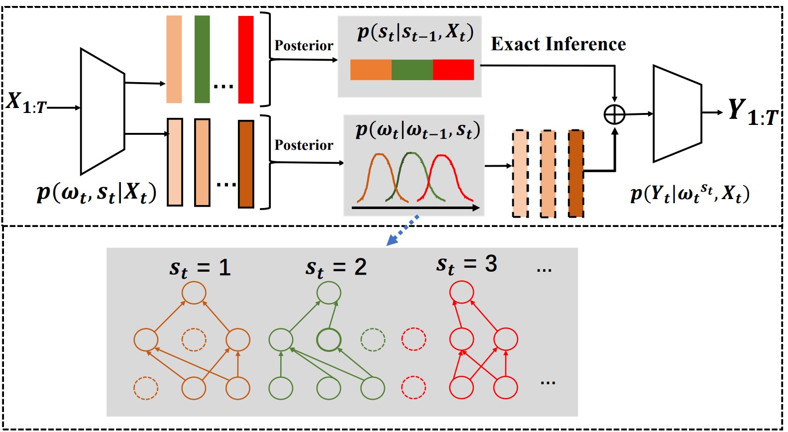
Figure 1. Overview of the T-SaS method. We derive a probabilistic framework to infer the distribution shift and modulate the adaptive model simultaneously. Input $\mathbf{X}_{1:T}$ is feed into a neural network to infer two variables, i.e., the latent change point variable $\bm{s}_{t}$ and model posterior parameters $\bm{\omega}_{t}$. The change point variable is conditioned on $\bm{s}_{t-1}$ and $\mathbf{X}_{t-1}$ which encodes the time-dependent relations and can be calculated by exact inference. $\bm{\omega}_{t}$ is sampled with a dynamic masking-based strategy to determine the model prediction $p(\mathbf{Y}_{t}|\mathbf{X}_{t},\bm{\omega}_{t})$.

Note that discrete change variables $s_{t}$ influence the adaptive model parameters $\bm{\omega}$ and are indicative for sudden distribution shift. Intuitively, $s_{t}$ depends on previous change variable $s_{t-1}$ as time-varying data usually maintains a local smoothness property for time duration (Ansari et al., 2021), but also depends on previous observation $\mathcal{D}_{t-1}$. This means the variable $s_{t}$ may be triggered by signals from the environment. To better express the flexible transition of the change point variable, we reformulate Eq.2 as follows:

(3) $$p(\bm{\omega}_{t},\bm{s}_{t}|\mathcal{D}_{1;t})$$

$$\propto p(\mathcal{[}D_{t}|\bm{\omega},s_{t}])p(\bm{\omega},s_{t}|\mathcal{D}_{1:t-1})p(s_{t}|\mathcal{D}_{1:t-1},s_{t-1}).$$

Summing over time steps, we can reformulate each term in Eq.2 using Markov Chain to model the joint distribution as:

(4) $$p(\mathcal{D}_{1:T},\bm{\omega}_{1:T},\bm{s}_{1:T})$$

$$= \prod_{t=2}^{T}p(\mathcal{D}_{t}|\mathcal{\omega}_{t},\bm{s}_{t})p(\bm{\omega}_{t}|\bm{\omega}_{t-1},\bm{s}_{t})p(\bm{s}_{t}|\bm{s}_{t-1},\mathcal{D}_{t-1}).$$

In this framework, with $\mathcal{D}_{t}$ being modeled as $p(\mathcal{D}_{t}|\mathcal{\bm{\omega}}_{t},\bm{s}_{t})$, shifts in data distribution can be encoded with change point indicator $\bm{s}_{t}$ for the problem of evolving data generalization. Next, we will go into details on the detection module with detected shifts.

2.2. Change Point Detection for Data Stream

When training with a complex dataset, the posterior distribution is intractable and needs to be inferred (Dong et al., 2020). A common approach to learning latent variables is to maximize the evidence lower bound (ELBO) on the log marginal likelihood (Nguyen et al., 2017). This is given by $\log p(\mathcal{D})\leq\mathbb{E}_{q_{\bm{\phi}}(\bm{w},\bm{s})}[\log p_{\bm{\theta}}(\mathcal{D},\bm{w},\bm{s})-\log q_{\bm{\phi}}(\bm{w},\bm{s}|\mathcal{D})]$, where $p_{\bm{\theta}}(\mathcal{D},\bm{w},\bm{s})$ shows the generative process and $q_{\bm{\phi}}(\bm{w},\bm{s}|\mathcal{D})$ is an approximation posterior. We define the prior distribution in Eq.4 for change point variable $\bm{s}$ and model parameter $\bm{w}$ as:

(5) $$p(\bm{w}^{\bm{s}_{t}}_{t})\sim\mathcal{N}(\bm{w}^{\bm{s}_{t}}|\bm{\mu}^{\bm{s}_{t}},\bm{\Sigma}^{\bm{s}_{t}}),$$

$$p(\bm{s}_{t})\sim Cat(\bm{s}_{t}|S(f(\bm{s}_{t-1},\mathcal{D}_{t-1}))),$$

where $\mathcal{N}$($\cdot$) is a multivariate Gaussian distribution with mean and Var as $\bm{\mu}^{\bm{s}_{t}}$ and $\bm{\Sigma}^{\bm{s}_{t}}$. $f$ is an non-linear function (MLPs), $\mathcal{C}at$($\cdot$) denotes a categorical distribution and S($\cdot$) is a softmax function.

To approximate the prior distribution, we propose to use variational inference to learn an approximated posterior distribution $q_{\bm{\phi}}$ over the latent variable and formulate it as:

(6) $$q_{\bm{\phi}}(\bm{w},\bm{s}|\bm{x})=p_{\bm{\theta}}(\bm{s}|\bm{x})q_{\bm{\phi}}(\bm{w}|\bm{x},\bm{s}),$$

where $p_{\bm{\omega}}(\bm{s}|\mathcal{x})$ is the exact posterior computed by forward-backward algorithm (Dong et al., 2020) and $q_{\bm{\phi}}(\bm{w}|\bm{x},\bm{s})$ is an approximated posterior. At this moment, we assume the distribution of $q_{\bm{\phi}}(\bm{w}|\bm{x},\bm{s})$ is given. Optimizing the variational parameters $\bm{\phi}$ corresponds to minimizing the ELBO at each time step $t$:

(7) $$\mathcal{L}(\bm{\phi}_{t})= \mathbb{E}_{q_{\bm{\phi}_{t}}(\bm{w},\bm{s}|\mathbf{X})p_{\bm{\omega}}(\bm{s}|\bm{w},\mathbf{X})}[-\log p(\mathbf{X}_{t}|\bm{w}^{\bm{s}_{t}}_{t})p_{\bm{\omega}}(\bm{s}_{t}|\mathbf{X}_{t})]$$

$$+\log q_{\bm{\phi}_{t}}(\bm{w},\bm{s}|\mathbf{X})p_{\bm{\omega}}(\bm{s}_{t}|\mathbf{X}_{t})$$

$$= \mathbb{E}_{q_{\bm{\phi}_{t}}(\bm{w},\bm{s}|\mathbf{X})}[-\log p(\mathcal{D}_{t}|\bm{w}^{\bm{s}_{t}}_{t})]$$

$$+\mathbf{KL}(q_{\bm{\phi}_{t}}(\bm{w}^{\bm{s}_{t}}|\bm{X},\bm{s})||q_{\bm{\phi}_{t-1}}(\bm{w}^{\bm{s}_{t}}|\bm{X},\bm{s})),$$

where the likelihood term $\mathbb{E}_{\mathbf{X}\thicksim{\mathcal{D}_{t}}}[\log p(\mathbf{X}_{t}|\bm{w}_{t},\mathbf{X}_{t-1})]$ can be computed using the forward variable $\alpha_{t}(\bm{s}_{t})$ by marginalizing out the change point variable $\bm{s}_{t}$,

(8) $$p(\mathbf{X}_{1:T},\bm{w}_{1:T})=\sum_{\bm{s}_{t}}\alpha_{t}(\bm{s}_{t})=\sum_{t=2}^{T}\sum_{j,k}\gamma_{t}(j,k)[\log B_{t}(k)A_{t}(j,k)],$$

where $A_{(}j,k)=p(\bm{s}_{t}=j|\bm{s}_{t-1}=k,\mathbf{X}_{t-1})$ and $B_{t}(k)=p(\mathbf{X}_{t}|\bm{\omega_{t}})\cdot\\ p(\bm{\omega}_{t}|\omega_{t-1},\bm{s}_{t}=k)$. Here, change point variables can be calculated from exact inference. The ELBO can be approximated via stochastic gradient ascent given that $q_{\bm{\phi}_{t}}(\bm{w}^{\bm{s}_{t}}|\bm{X},\bm{s})$ is reparameterizable.

2.3. Structure Adaptation With Change Points

To improve the adaption on a sequence of evolving data distribution, the continual learner is equipped with a mixture of dynamically updated model parameters $\{\bm{\omega}_{t}^{\bm{s}_{t}}\}_{\bm{s}_{t}=1}^{K}$, where $K$ is the number of categorical data numbers. Each change point variable $\bm{s}_{t}$ is associated with a cluster of similar data distributions, and we define $\bm{\omega}_{t}^{\bm{s}_{t}}$ as the specific model parameters. Notably, our model requires that parameters can be dynamically updated as future similar data emerges. To allow room for constantly emerging data, the model parameters are often easily overparameterized (Ostapenko et al., 2021). To regularize the model parameter to maintain a small size and be immune to overfit, we assume that only a small number of neurons should be activated for each distribution. Given the change point variable $\bm{s}_{t}$, the neural network can dynamically search for a shift-oriented subnetwork. The sparsification rather than using the original network are under two reasons: 1) Lottery Tickets Hypothesis (Frankle and Carbin, 2018) verifies that a subnetwork can perform as well as a whole network, which is also verified by current findings on model compression; 2) subnetwork can facilitate the learning of evolving network structure, therefor be more robust to distribution shift.

To be specific, for each specific model parameter $\bm{\omega}^{\bm{s}_{t}}_{t}$, we decompose it as $\bm{\omega}^{\bm{s}_{t}}_{t}=\bm{\omega}_{t}\odot\bm{m^{\bm{s}_{t}}}_{t}$, an element-wise multiplication of a global model parameter $\bm{\omega}_{t}$ and a shift-driven mask matrix $\bm{m^{\bm{s}_{t}}}_{t}$. Deriving the exact posterior distribution for the model parameter $\bm{w}$ is intractable due to the nonlinearities of the model. Here, we assume a Gaussian distribution with parameters $\{\bm{\mu}_{t}^{\bm{s}_{t}},\mathbf{\Sigma}_{t}^{\bm{s}_{t}}\}$ as the posterior distribution of model parameters $\bm{w}$: $q_{\bm{\phi}}(\bm{w}_{t})=\mathcal{N}(\bm{w}^{\bm{s}_{t}}|\bm{\mu}^{\bm{s}_{t}},\bm{\Sigma}^{\bm{s}_{t}})$.

Following the principle of variational continual learning (Nguyen et al., 2017), we assume that the prior of $\bm{\omega}_{t}^{s_{k}}$ is given by the variational posterior of $\bm{\omega}_{t-1}^{s_{k}}$, i.e., $\bm{\mu}_{t}^{\bm{s}_{t}}=\bm{\mu}_{t-1}^{s_{t-1}}$, $\mathbf{\Sigma}_{t}^{\bm{s}_{t}}=\mathbf{\Sigma}_{t-1}^{s_{t-1}}$.

Besides, keep in mind that $\bm{\bm{m}_{t}^{s_{t}}}$ is a learnable model mask parameter that determines which neurons should be activated or set as zeros. To simplify our exposition, we omit script $\bm{s}_{t}$ To model the sparsity property of mask matrix, we define the prior distribution of $p(\bm{m}^{s_{t}})$ using the India buffer process (Nguyen et al., 2017) : $\bm{m}\sim IBP(\alpha)$, where $\alpha$ is the hyperparameters that can control the number of nonzero elements in $\bm{m}$. Specifically, its truncated stick-breaking process for each element in $\bm{m}$ can be denoted as :

(9) $$v_{k}\sim Beta(\alpha,1),\pi_{k}=\prod_{i=1}^{K}v_{i},B_{d,k}\sim Bern(\pi_{k}),$$

where $K$ is the truncated level and $\alpha$ controls the value of $K$. To represent the approximated posterior of $m$, we define it as $q(\bm{m})=q(\bm{m}|v)q(v)$. Corresponding to the Beta-Bernoulli hierarchy of Eq.9, we use the conditional factorized variational posterior family:

(10) $$q(\bm{m}|v)=\prod_{d-1}^{D}\prod_{k-1}^{K}Bern(m_{d,k}|h_{d,k}),$$

where $h_{d,k}=\sigma(\rho_{d,k}+logit(\pi_{k}))$ and $q(v)=\prod_{k=1}^{K}Beta(v_{k}|v_{k,1},v_{k,2})$. Consequently, we obtain a set of learnable variational parameters $\{v_{k,1},v_{k,2},\{\mu_{d,k},\Sigma_{d,k},\rho_{d,k}\}\}$.

3. Experiment

3.1. Experimental Setup

3.1.1. Data Description

We select both synthetic and real-world benchmark dataset to validate the ‘shift detecting’ and ‘shift adapting’ properties of the proposed method. Experiments are conducted on 3 mode system (Ansari et al., 2021) and Dancing bees (Oh et al., 2008). Second, we evaluate the ability of the proposed method in adapting to evolving data streams. Experiments are conducted on two tasks, the forecasting task (only the evolving feature $\mathbf{X}_{1:T}$ is given to predict $\mathbf{X}_{t+1}$) and the classification task (learn a mapping from $\mathbf{X}_{t}$ to $\mathbf{Y}_{t}$. Specifically, we use four benchmark forecasting datasets (Alexandrov et al., 2020) including traffic, exchange, solar and electricity, where various seasonality patterns, e.g., daily, weekly or monthly are shown, and two challenge classification datasets MG_1C_2D and optdigits following (Souza et al., 2015).

3.1.2. Baselines algorithms

Since there are limited studies working on the same setting with ours, we compared our method with representative continual learning methods, domain adaptation methods via evolving shifted data and other competitive baselines. Specifically, we conduct experiments on both forecasting and classification problems on evolving data. (1) JT (joint training): a naive baseline that train on all the available data ever seen $D_{1,T}$. (2) Adaptive RNN (AdaRNN) (Du et al., 2021): a two-stage method that follow a ‘segment-adapt’ principle for the evolving shifted data. (3) Meta-learning via online change point analysis (MOCA) (Harrison et al., 2020): an approach which augments a meta-learning algorithm with a differentiable Bayesian change point detection scheme.

3.2. Experiment Results and Analysis

3.2.1. Shift Detection Comparison

Table 1. Comparison of effectiveness on shift detection. Accuracy, NMI, ARI denote the Normalized Mutual Information, the Adjusted Rand Index and segmentation accuracy metrics.

		Bouncing Ball	3 mode system	Dancing bees
Accuracy	MOCA	$0.93\pm 0.02$	$0.94\pm 0.04$	$0.71\pm 0.03$
	AdaRNN	$0.93\pm 0.05$	$0.90\pm 0.10$	$0.68\pm 0.01$
	T-SaS	0.96 $\pm$ 0.05	0.97 $\pm$ 0.00	0.73 $\pm$ 0.14
NMI	MOCA	$0.81\pm 0.00$	$0.83\pm 0.06$	$0.30\pm 0.04$
	AdaRNN	$0.79\pm 0.01$	$0.79\pm 0.13$	$0.57\pm 0.01$
	T-SaS	0.82 $\pm$ 0.011	0.90 $\pm$ 0.02	0.61 $\pm$ 0.01
ARI	MOCA	$0.85\pm 0.02$	$0.89\pm 0.01$	$0.38\pm 0.01$
	AdaRNN	$0.84\pm 0.02$	$0.85\pm 0.11$	$0.47\pm 0.01$
	T-SaS	0.86 $\pm$ 0.00	0.94 $\pm$ 0.01	0.54 $\pm$ 0.11

Experiments in this section are designed to analyze the shift detection behavior of our proposed method. Experimental results are shown in Table 1 and we also represent the visualization in Figure 2 and Figure 3, respectively. Experimental results show that our method achieves significant improvements over the baselines. From Figure 2, we observe that AdaRNN apparently struggles to model long-term sequence data and results in over-segmentation. Additionally, we observe AdaRNN performs a large variance than MOCA and our method. The observation shows its inefficiency to detect the shift point for AdaRNN model, especially for complex sequences. It is also obvious that MOCA identifies a fluctuated detection in a three mode system dataset for its inefficiency to model long-term motion patterns. The observation validates the effectiveness of detecting complex patterns and segmenting the long-term motions for our T-SaS method.

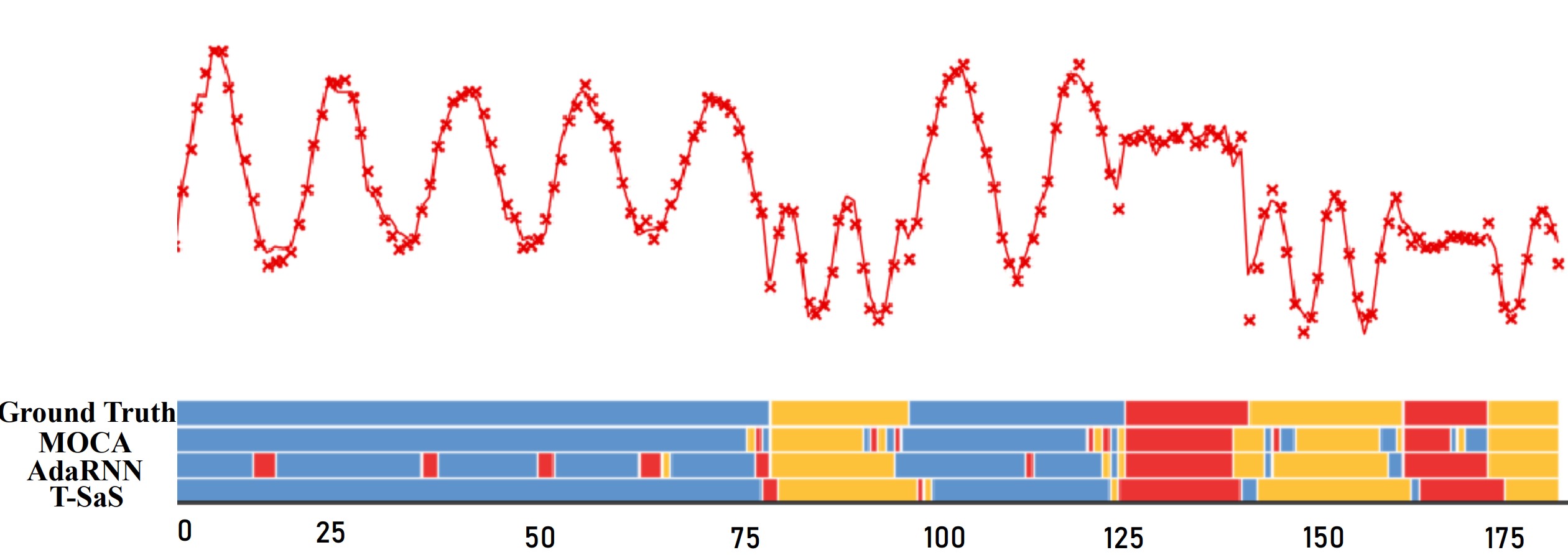
Figure 2. Segmentation visualization on the three mode system dataset.

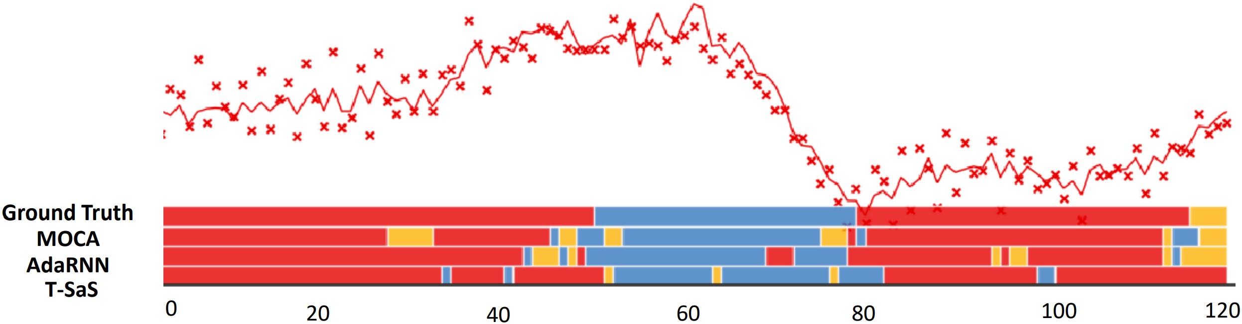
Figure 3. Segmentation visualization on the dancing bee dataset.

From Figure.3, it is obvious that MOCA fails to identify long segment duration and results in spurious short-term patterns. Differently, our method is able to segment the long-term patterns quite well by taking the advantage of a latent time duration variable. This observation verifies our motivation that a latent time duration variable could benefit the learning of long-term patterns.

3.2.2. Drift Adaptation Comparison.

In this part, experiments are designed to understand if and how the proposed method can adapt to the shifted streaming data. Experiments on forecasting and classification tasks are shown in Figure 4 and Figure 5, respectively.

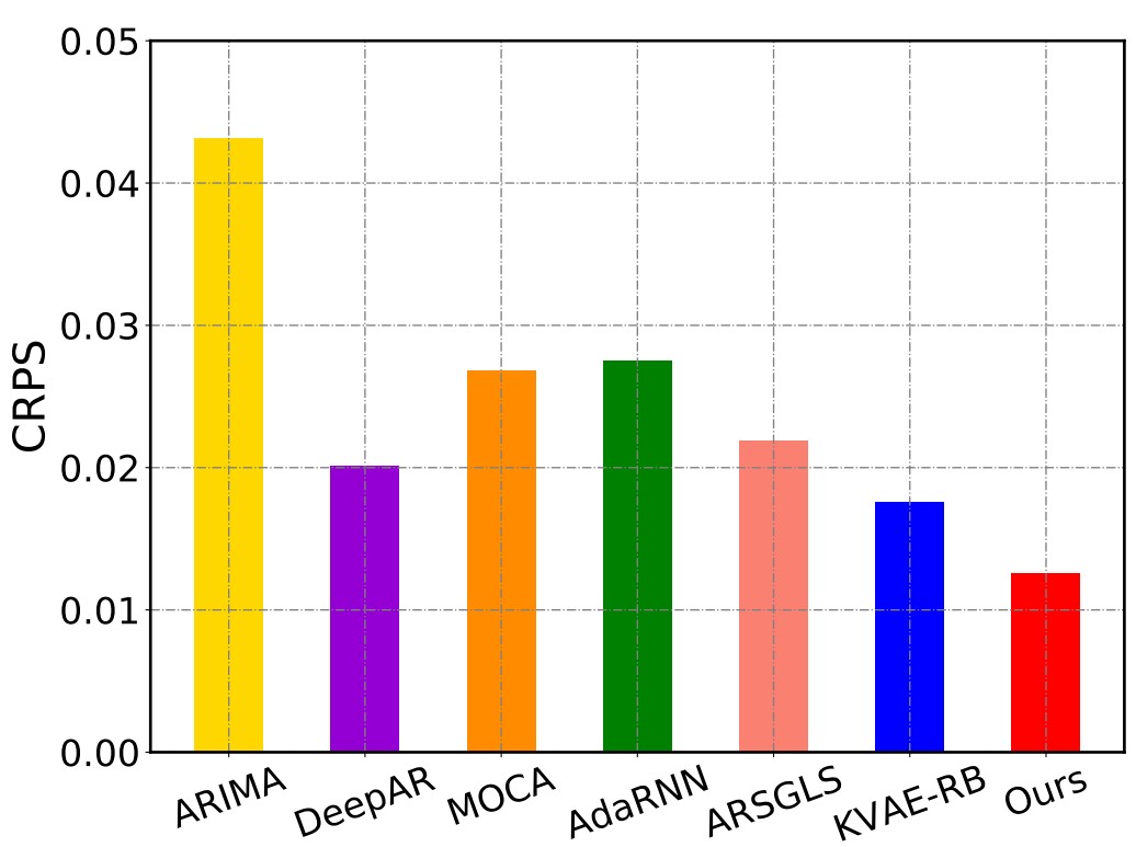
(a)

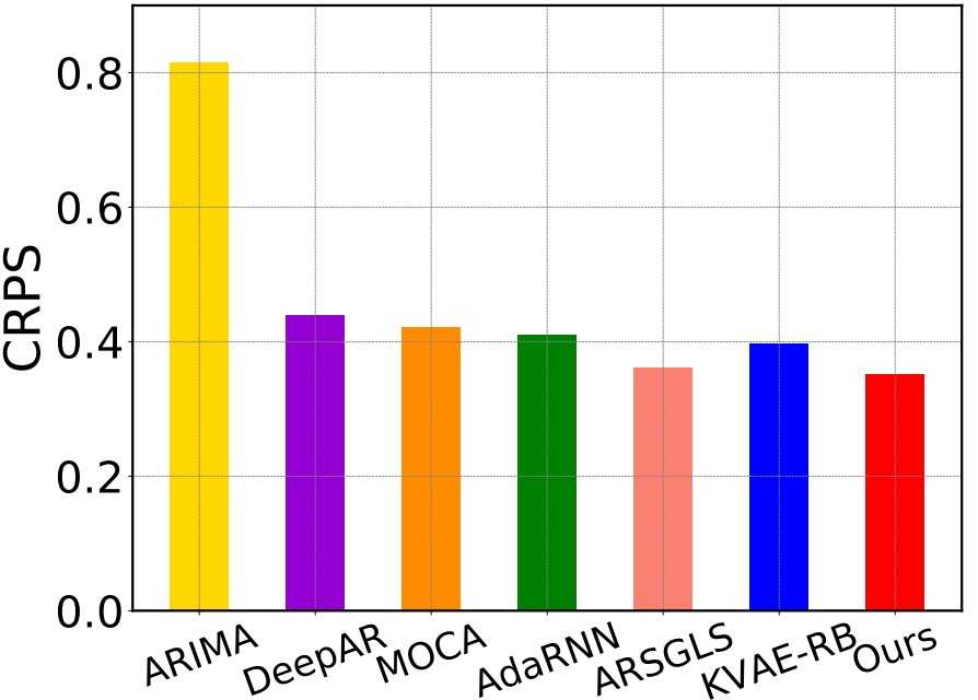
(b)

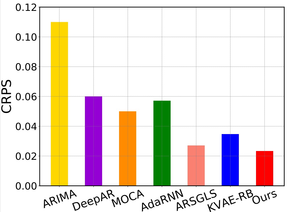
(c)

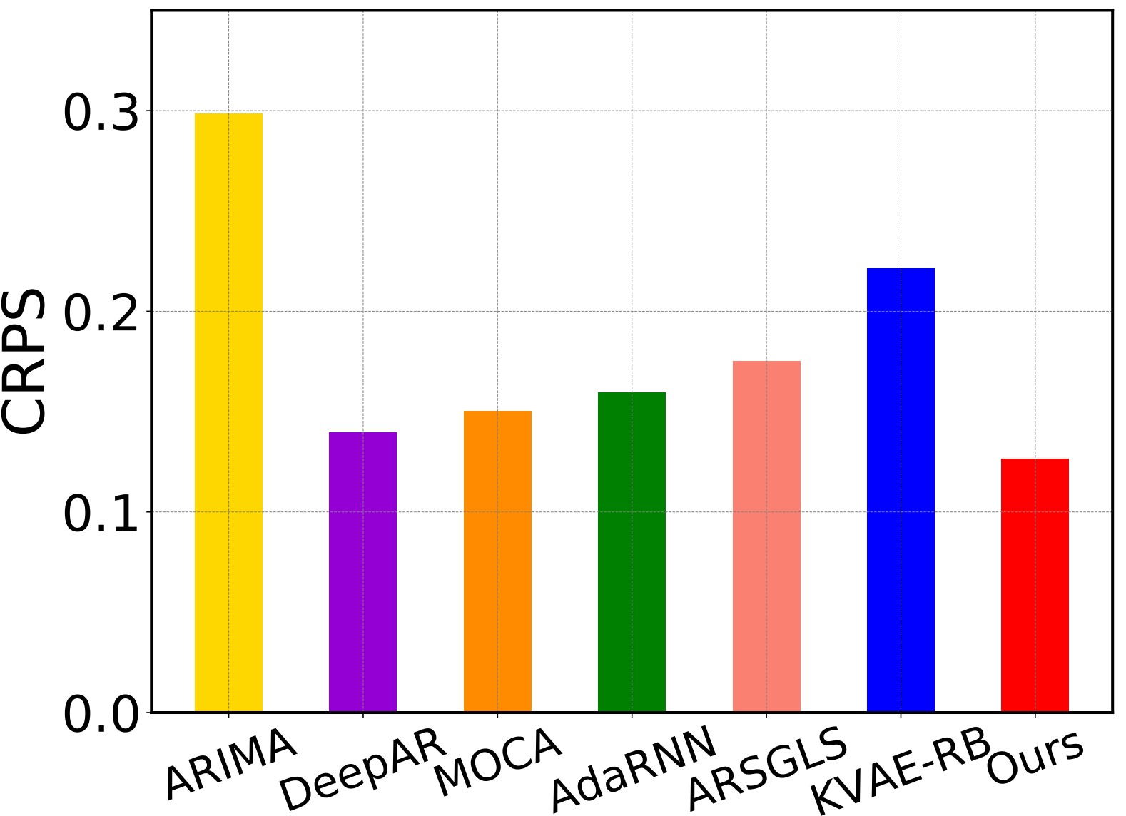
(d)

Figure 4. Forecasting performance across datasets. The lower the value, the better the performance.

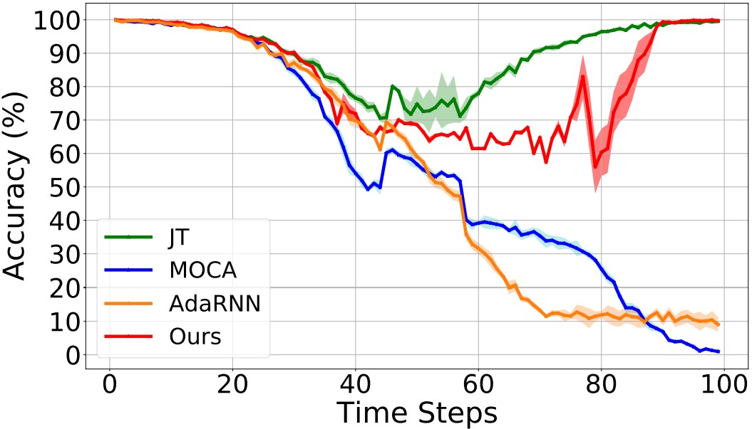
(a)

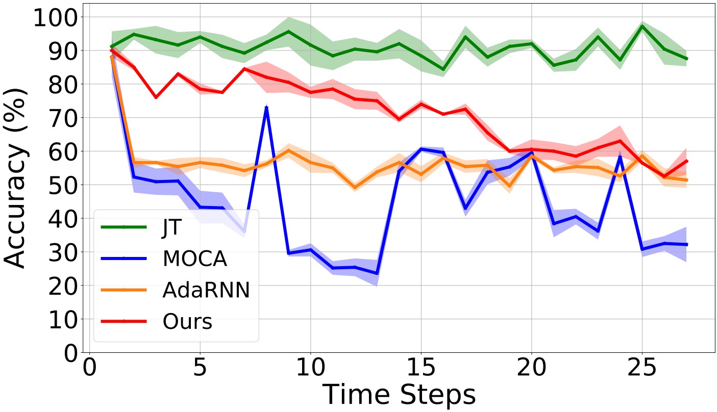
(b)

Figure 5. Classification results through timelines.

From Figure 4, We first observe our method outperforms all the baselines over all four benchmark datasets. Our method simultaneously infers these distribution shifts and adapts the model to the detected changes with a dynamic model structure. Besides, AdaRNN and MOCA show relatively unsatisfactory performance. The main reason is AdaRNN and MOCA adapt to shifted data with global sharing model parameters. Parameter sharing facilitates the transfer of invariance knowledge while penalizing the learning of specialized information. Figure 5 shows that our method achieves significant improvements over the baselines and is even comparable with the Joint Training (JT) method (upper bound of the setting). Moreover, the margin between our method and baselines, i.e., MOCA and AdaRNN continually increases, indicating our dynamic model architecture can enrich the model expression capacity.

4. Conclusion

This paper addresses the problem of modeling low-source streaming data where data shift boundaries are not given. Additionally, we expand the assumptions regarding distribution shifts to include sudden and irregular patterns. In addition, we train a specific mask matrix to dynamically route a sparse network from the full network. We propose an adaptive model for the evolving data by introducing the Bayesian framework with change point variables. Experimental results on both forecasting and classification tasks demonstrate the effectiveness of the proposed method.

References

- (1)
- Alexandrov et al. (2020) Alexander Alexandrov, Konstantinos Benidis, Michael Bohlke-Schneider, Valentin Flunkert, Jan Gasthaus, Tim Januschowski, Danielle C Maddix, Syama Sundar Rangapuram, David Salinas, Jasper Schulz, et al. 2020. GluonTS: Probabilistic and Neural Time Series Modeling in Python. J. Mach. Learn. Res. 21, 116 (2020), 1–6.
- Ansari et al. (2021) Abdul Fatir Ansari, Konstantinos Benidis, Richard Kurle, Ali Caner Turkmen, Harold Soh, Alexander J Smola, Bernie Wang, and Tim Januschowski. 2021. Deep Explicit Duration Switching Models for Time Series. Advances in Neural Information Processing Systems 34 (2021), 29949–29961.
- De Lange et al. (2021) Matthias De Lange, Rahaf Aljundi, Marc Masana, Sarah Parisot, Xu Jia, Aleš Leonardis, Gregory Slabaugh, and Tinne Tuytelaars. 2021. A continual learning survey: Defying forgetting in classification tasks. IEEE transactions on pattern analysis and machine intelligence 44, 7 (2021), 3366–3385.
- Dong et al. (2020) Zhe Dong, Bryan Seybold, Kevin Murphy, and Hung Bui. 2020. Collapsed amortized variational inference for switching nonlinear dynamical systems. In International Conference on Machine Learning. PMLR, 2638–2647.
- Du et al. (2021) Yuntao Du, Jindong Wang, Wenjie Feng, Sinno Pan, Tao Qin, Renjun Xu, and Chongjun Wang. 2021. Adarnn: Adaptive learning and forecasting of time series. In Proceedings of the 30th ACM International Conference on Information & Knowledge Management. 402–411.
- Frankle and Carbin (2018) Jonathan Frankle and Michael Carbin. 2018. The lottery ticket hypothesis: Finding sparse, trainable neural networks. arXiv preprint arXiv:1803.03635 (2018).
- Harrison et al. (2020) James Harrison, Apoorva Sharma, Chelsea Finn, and Marco Pavone. 2020. Continuous meta-learning without tasks. Advances in neural information processing systems 33 (2020), 17571–17581.
- Liu et al. (2020) Hong Liu, Mingsheng Long, Jianmin Wang, and Yu Wang. 2020. Learning to adapt to evolving domains. Advances in Neural Information Processing Systems 33 (2020), 22338–22348.
- Nguyen et al. (2017) Cuong V Nguyen, Yingzhen Li, Thang D Bui, and Richard E Turner. 2017. Variational continual learning. arXiv preprint arXiv:1710.10628 (2017).
- Oh et al. (2008) Sang Min Oh, James M Rehg, Tucker Balch, and Frank Dellaert. 2008. Learning and inferring motion patterns using parametric segmental switching linear dynamic systems. International Journal of Computer Vision 77, 1 (2008), 103–124.
- Ostapenko et al. (2021) Oleksiy Ostapenko, Pau Rodriguez, Massimo Caccia, and Laurent Charlin. 2021. Continual learning via local module composition. Advances in Neural Information Processing Systems 34 (2021), 30298–30312.
- Ren et al. (2021b) Weijeiying Ren, Kunpeng Liu, Tianxiang Zhao, and Yanjie Fu. 2021b. Fair and effective policing for neighborhood safety: understanding and overcoming selection biases. Frontiers in big data 4 (2021), 787459.
- Ren et al. (2022b) Weijieying Ren, Lei Wang, Kunpeng Liu, Ruocheng Guo, Lim Ee Peng, and Yanjie Fu. 2022b. Mitigating popularity bias in recommendation with unbalanced interactions: A gradient perspective. In 2022 IEEE International Conference on Data Mining (ICDM). IEEE, 438–447.
- Ren et al. (2022a) Weijieying Ren, Pengyang Wang, Xiaolin Li, Charles E Hughes, and Yanjie Fu. 2022a. Semi-supervised drifted stream learning with short lookback. In Proceedings of the 28th ACM SIGKDD Conference on Knowledge Discovery and Data Mining. 1504–1513.
- Ren et al. (2017) Weijieying Ren, Lei Zhang, Bo Jiang, Zhefeng Wang, Guangming Guo, and Guiquan Liu. 2017. Robust mapping learning for multi-view multi-label classification with missing labels. In Knowledge Science, Engineering and Management: 10th International Conference, KSEM 2017, Melbourne, VIC, Australia, August 19-20, 2017, Proceedings 10. Springer, 543–551.
- Ren et al. (2021a) Xiaoying Ren, Jing Jiang, Ling Min Serena Khoo, and Hai Leong Chieu. 2021a. Cross-Topic Rumor Detection using Topic-Mixtures. In Proceedings of the 16th Conference of the European Chapter of the Association for Computational Linguistics: Main Volume. 1534–1538.
- Ren et al. (2018) Xiaoying Ren, Linli Xu, Tianxiang Zhao, Chen Zhu, Junliang Guo, and Enhong Chen. 2018. Tracking and forecasting dynamics in crowdfunding: A basis-synthesis approach. In 2018 IEEE International Conference on Data Mining (ICDM). IEEE, 1212–1217.
- Shen et al. (2023) Qinghua Shen, Weijieying Ren, and Wei Qin. 2023. Graph Relation Aware Continual Learning. arXiv preprint arXiv:2308.08259 (2023).
- Souza et al. (2015) Vinícius MA Souza, Diego F Silva, João Gama, and Gustavo EAPA Batista. 2015. Data stream classification guided by clustering on nonstationary environments and extreme verification latency. In Proceedings of the 2015 SIAM International Conference on Data Mining. SIAM, 873–881.
- Wang et al. (2022) Lei Wang, Ee-Peng Lim, Zhiwei Liu, and Tianxiang Zhao. 2022. Explanation guided contrastive learning for sequential recommendation. In Proceedings of the 31st ACM International Conference on Information & Knowledge Management. 2017–2027.
- Wang and Deng (2018) Mei Wang and Weihong Deng. 2018. Deep visual domain adaptation: A survey. Neurocomputing 312 (2018), 135–153.
- Wilson and Cook (2020) Garrett Wilson and Diane J Cook. 2020. A survey of unsupervised deep domain adaptation. ACM Transactions on Intelligent Systems and Technology (TIST) 11, 5 (2020), 1–46.
- Xu et al. (2018) Linli Xu, Wenjun Ouyang, Xiaoying Ren, Yang Wang, and Liang Jiang. 2018. Enhancing Semantic Representations of Bilingual Word Embeddings with Syntactic Dependencies.. In IJCAI. 4517–4524.
- Zhang et al. (2021) Youshan Zhang, Hui Ye, and Brian D Davison. 2021. Adversarial reinforcement learning for unsupervised domain adaptation. In Proceedings of the IEEE/CVF Winter Conference on Applications of Computer Vision. 635–644.
- Zhao et al. (2018) Tianxiang Zhao, Guiquan Liu, Chao Ma, Enhong Chen, et al. 2018. Zero-shot learning: An energy based approach. In 2018 IEEE International Conference on Data Mining (ICDM). IEEE, 797–806.
- Zhao et al. (2020) Tianxiang Zhao, Lemao Liu, Guoping Huang, Huayang Li, Yingling Liu, Liu GuiQuan, and Shuming Shi. 2020. Balancing quality and human involvement: An effective approach to interactive neural machine translation. In Proceedings of the AAAI Conference on Artificial Intelligence, Vol. 34. 9660–9667.
- Zhao et al. (2022a) Tianxiang Zhao, Dongsheng Luo, Xiang Zhang, and Suhang Wang. 2022a. On consistency in graph neural network interpretation. arXiv preprint arXiv:2205.13733 (2022).
- Zhao et al. (2022b) Tianxiang Zhao, Dongsheng Luo, Xiang Zhang, and Suhang Wang. 2022b. TopoImb: Toward Topology-level Imbalance in Learning from Graphs. In Learning on Graphs Conference. PMLR, 37–1.
- Zhao et al. (2023a) Tianxiang Zhao, Dongsheng Luo, Xiang Zhang, and Suhang Wang. 2023a. Faithful and Consistent Graph Neural Network Explanations with Rationale Alignment. ACM Transactions on Intelligent Systems and Technology(TIST) (2023).
- Zhao et al. (2023b) Tianxiang Zhao, Dongsheng Luo, Xiang Zhang, and Suhang Wang. 2023b. Towards Faithful and Consistent Explanations for Graph Neural Networks. In Proceedings of the Sixteenth ACM International Conference on Web Search and Data Mining. 634–642.
- Zhao et al. (2023c) Tianxiang Zhao, Wenchao Yu, Suhang Wang, Lu Wang, Xiang Zhang, Yuncong Chen, Yanchi Liu, Wei Cheng, and Haifeng Chen. 2023c. Skill Disentanglement for Imitation Learning from Suboptimal Demonstrations. KDD (2023).
- Zhao et al. (2022c) Tianxiang Zhao, Xiang Zhang, and Suhang Wang. 2022c. Synthetic over-sampling for imbalanced node classification with graph neural networks. arXiv preprint arXiv:2206.05335 (2022).