Directionality-Aware Mixture Model Parallel Sampling for
Efficient Linear Parameter Varying Dynamical System Learning

Abstract

The Linear Parameter Varying Dynamical System (LPV-DS) is an effective approach that learns stable, time-invariant motion policies using statistical modeling and semi-definite optimization to encode complex motions for reactive robot control. Despite its strengths, the LPV-DS learning approach faces challenges due to the curse of dimensionality, impacting model and computational efficiency. To address this, we introduce the Directionality-Aware Mixture Model (DAMM), a novel statistical model that applies the Riemannian metric on the n-sphere $\mathbb{S}^{n}$ to efficiently blend non-Euclidean directional data with $\mathbb{R}^{m}$ Euclidean states. Additionally, we develop a hybrid Markov chain Monte Carlo technique that combines Gibbs Sampling with Split/Merge Proposals, allowing for parallel computation to drastically speed up inference. Our extensive empirical tests demonstrate that LPV-DS integrated with DAMM achieves higher reproduction accuracy, better model efficiency, and near real-time/online learning compared to standard estimation methods on various datasets. Lastly, we demonstrate its suitability for incrementally learning multi-behavior policies in real-world robot experiments.
Code: https://github.com/damm-2023/damm

I Introduction

Safe integration of robots into human workspaces requires the ability to adapt and replan in response to changing environments and constraints. Traditional path planning approaches, assuming a known environment and robot dynamics, face challenges when confronted with uncertainties and perturbations during operation [1, 2, 3]. In contrast, Dynamical System (DS)-based motion policies leverage redundancy of solutions in dynamic environments, embedding an infinite set of feasible solutions in a single control law to overcome environmental uncertainties and perturbations [4]. Furthermore, stability conditions can be introduced as constraints in the learning of DS, providing a closed-form analytical solution to trajectory planning, with theoretical guarantees such as stability and convergence [5, 6].

Our focus is on learning stable, time-independent motion policies from limited demonstrations, emphasizing i) distinct behaviors or state-space coverage (as shown in Fig. 7), ii) minimal training data, and iii) model and computational efficiency for real-time incremental learning and control. While recent neural network (NN) based formulations for stable DS motion policies show promising results in encoding highly non-linear trajectories; as adopting normalizing flows [7], euclideanizing flows [8] or via contrastive learning [9]; given their black-box nature they are not easily applicable to incremental near real-time learning contexts. Such NN-based methods need many trajectories and substantial computation time to reach stable solutions, typically assuming single-behavior trajectories. Interestingly, the seminal works on the Linear Parameter Varying Dynamical System (LPV-DS) formulation and its Gaussian Mixture Model (GMM) based learning frameworks [6, 10, 4] can achieve objectives i-ii), but face growing model and computation inefficiencies with more data and trajectory complexity, hindering its use in incremental or end-to-end learning. To address this, in this paper, we revisit the LPV-DS formulation and the state-of-the-art Physically Consistent (PC)-GMM learning scheme [10] (Section II). In particular, we stress that although PC-GMM effectively creates physically meaningful GMM fits for highly non-linear trajectory data, it struggles with the curse of dimensionality due to a) its dependency on similarity metrics and b) non-parallelizable sampling inference process.

Contributions: In tackling the aforementioned challenges, we introduce the Directionality-Aware Mixture Model (DAMM). Inspired by prior work on clustering spherical data on Riemannian manifolds [11], the DAMM formulation augments state variables $\xi\in\mathbb{R}^{d}$ with directional information using a proper Riemannian metric on the directional data manifold, inherently capturing the directionality or the trend of motion along the reference trajectories (Section III-A). We then introduce a generative model (Section III-B) and a new parallel Markov chain Monte Carlo (MCMC) sampling scheme to find the optimal $K$ that can achieve online performance tailored to the DAMM formulation (Section III-C). These innovations offer computational efficiency, model efficiency and directional consistency for online estimation of LPV-DS motion policies from demonstrations in $<500ms$. As shown in Fig. 7, the DAMM-based LPV-DS successfully senses the directionality and identifies the linear portions of trajectories, resulting in physically-meaningful DS shown on the bottom right with less number of Gaussian $K$ than PC-GMM and with an unprecedented estimation time.

We evaluate our approach through extensive empirical validation, including benchmark comparisons on LASA datasets [12] and the PC-GMM dataset [10] (including 2D and 3D real trajectories) against PC-GMM and baseline sampling approaches, as well as real robot experiments (Section IV). We demonstrate that the DAMM-based LPV-DS framework exhibits enhanced capabilities in producing improved DS across various metrics, and achieves an order of magnitude faster rate of learning speed compared to its predecessor, allowing for efficient and nearly online learning performance.

To the best of our knowledge, this is the first DS learning framework that can be estimated in near real-time scale.

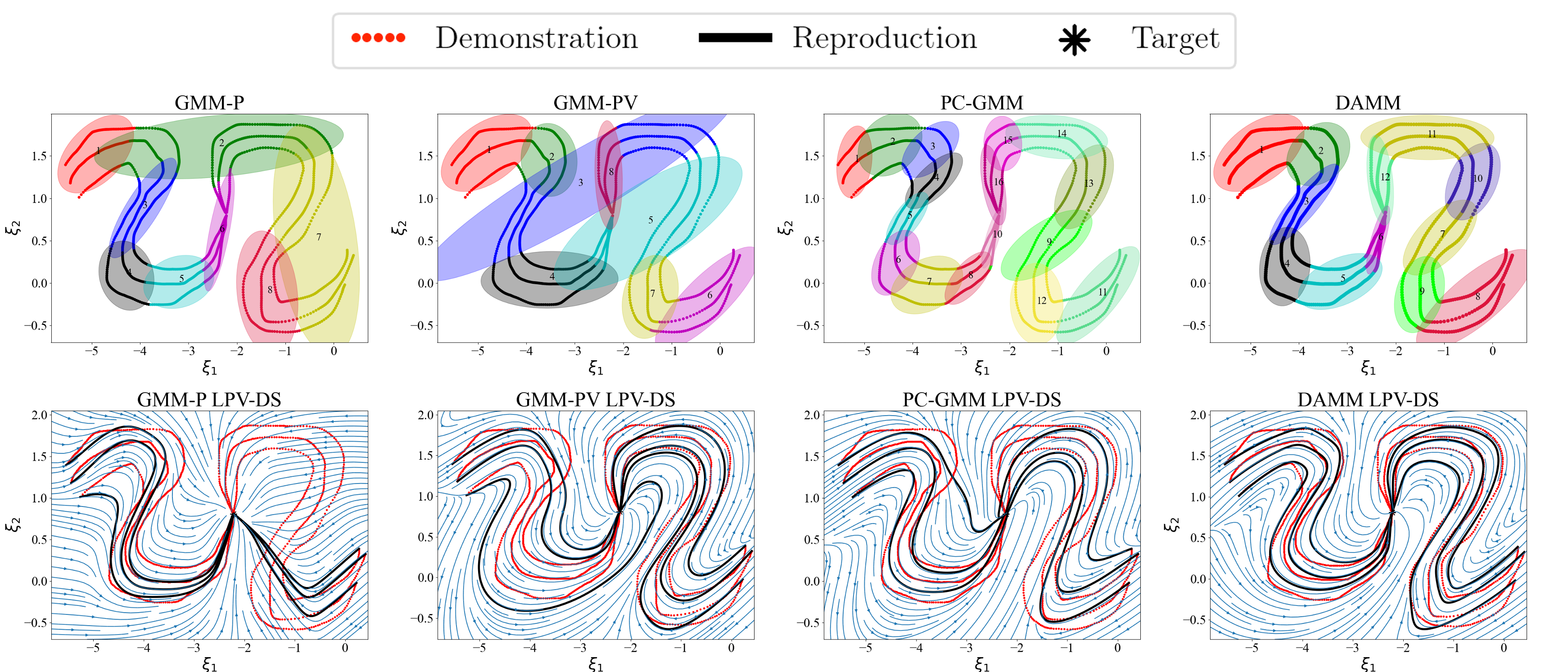
Figure 1: Comparison of clustering (top) and reproduction (bottom) results between the GMM-P (position only) LPV-DS, GMM-PV (position+velocity) LPV-DS, PC-GMM LPV-DS and DAMM LPV-DS on a multi-behavior trajectory obtained from [10]. Both GMM-P and GMM-PV are fitted via Gibbs Sampling. The computation times are 0.3, 0.5, 53 and 1.2 in seconds from left to right, and the number of components $K$ are 8, 8, 16 and 12. Notice the improved reproduction accuracy resulting from optimal GMM fitting via DAMM on the right column.

II Preliminaries

II-A The LPV-DS Formulation

Let $\xi,\dot{\xi}\in\mathbb{R}^{d}$ represent the kinematic robot state and velocity vectors. In the DS-based motion policy literature [4], $\dot{\xi}=f(\xi)$ is a first-order DS that describes a motion policy in the robot’s state space $\mathbb{R}^{d}$. The goal of DS-based learning from demonstration (LfD) is to infer $f(\xi):\mathbb{R}^{d}\rightarrow\mathbb{R}^{d}$ from data, such that any point $\xi$ in the state space leads to a stable attractor $\xi^{*}\in\mathbb{R}^{d}$, with $f(\xi)$ described by a set of parameters $\Theta$ and attractor $\xi^{*}\in\mathbb{R}^{d}$; mathematically $\dot{\xi}=f(\xi;\Theta,\xi^{*})\Rightarrow\lim_{t\to\infty}\|\xi-\xi^{*}\|=0$, i.e., the DS is globally asymptotically stable (GAS) [13].

Learning $\dot{\xi}=f(\xi)$ can be framed as a regression problem, where the inputs are the state variables $\xi$ and the outputs are the first-order time derivative $\dot{\xi}$. Such formulation gives rise to the utilization of statistical methods for estimating the parameters $\Theta$. However, standard regression techniques cannot ensure global asymptotic stability. To alleviate this, the LPV-DS approach was first introduced in the seminal work of [6] as a constrained Gaussian Mixture Regression (GMR) and then formalized as the untied GMM-based LPV-DS approach in [10], where a nonlinear DS is encoded as a mixture of continuous linear time-invariant (LTI) systems:

$$\quad\quad\dot{\xi}=f(\xi;\Theta)=\sum_{k=1}^{K}\gamma_{k}(\xi)\left(A_{k}\xi+b_{k}\right)$$ (1)

s.t. $$\,\,\left\{\begin{array}[]{l}\left(A_{k}\right)^{T}P+PA_{k}=Q_{k},Q_{k}=\left(Q_{k}\right)^{T}\prec 0\\ b_{k}=-A_{k}\xi^{*}\end{array}\right.$$

where $\gamma_{k}(\xi)$ is the state-dependent mixing function that quantifies the weight of each LTI system $(A_{k}\xi+b_{k})$ and $\Theta=\{\theta_{\gamma}\}_{\gamma=1}^{K}=\{\gamma_{k},A_{k},b_{k}\}_{k=1}^{K}$ is the set of parameters to learn. The constraints of the Eq. 1 enforce GAS of the result DS derived from a parametrized Lyapunov function $V(\xi)=(\xi-\xi^{*})^{T}P(\xi-\xi^{*})$ with $P=P^{T}\succ 0$ [10, 4].

To ensure GAS of Eq. 1, besides enforcing the Lyapunov stability constraints on the LTI parameters one must ensure that $0<\gamma_{k}(\xi)<1$ and $\sum_{k=1}^{K}\gamma_{k}(\xi)=1~{}\forall\xi\in\mathbb{R}^{d}$. As noted in [10], this is achieved by formulating $\gamma_{k}({\xi})=\frac{\pi_{k}\mathcal{N}({\xi}|\theta_{k})}{\sum_{j=1}\pi_{j}\mathcal{N}(\xi|\theta_{j})}$ as the a posteriori probability of the state $\xi$ from a GMM used to partition the nonlinear DS into linear components. Here, $K$ is the number of components corresponding to the number of LTIs, $\mathcal{N}({\xi}|\theta_{k})$ is the probability of observing ${\xi}$ from the $k$-th Gaussian component parametrized by mean and covariance matrix $\theta_{k}=\{\mu_{k},\Sigma_{k}\}$, and $\pi_{k}$ is the prior probability of an observation from this particular component satisfying $\sum_{k=1}^{K}\pi_{k}=1$.

In [10] a two-step estimation framework was proposed to estimate the GMM parameters $\Theta_{\gamma}=\{\pi_{k},\mu_{k},\Sigma_{k}\}_{k=1}^{K}$ and the DS parameters $\Theta_{DS}=\{A_{k},b_{k}\}_{k=1}^{K}$ forming $\Theta=\{\Theta_{\gamma},\Theta_{DS}\}$. First, given the set of reference trajectories $\mathcal{D}:=\{\xi^{\mathrm{ref}}_{i}\ \dot{\xi}^{\mathrm{ref}}_{i}\}_{i=1}^{N}$, where $i$ is the sequence order of the sampled states, a GMM is fit to the position variables of the reference trajectory, $\{\xi^{ref}_{i}\ \}_{i=1\dots N}$, to obtain $\Theta_{\gamma}$. The optimal number of Gaussians $K$ and their placement can be estimated by model selection via Expectation-Maximization or via Bayesian non-parametric estimation. Then, $\Theta_{DS}$ are learned through a semi-definite program minimizing reproduction accuracy subject to stability constraints [10, 4].

II-B Limitations of Vanilla and PC-GMM [10] for LPV-DS

Given a reference trajectory, one can interpret that each subsystem in Eq. 1 locally governs a portion of the trajectory. Recall that the learning of each subsystem derives from its corresponding Gaussian component, it is natural to assume that the statistical model places each Gaussian on near-linear segments. Such placement of Gaussians makes intuitive sense because Gaussian can be easily shaped in a long or slim manner to model linear trajectory. However, this is not always the case for standard GMM estimation techniques.

Vanilla GMM: In the first column of Fig. 7, we show an example of the GMM fit to the position $\xi$ only via standard Gibbs sampling, referred to as vanilla GMM-P. The clustering result fails to encapsulate the intrinsic motion of the original trajectory due to the lack of directionality, leading to an erroneous DS. Though one might be attempted to fit a GMM to the position and velocity $\xi,\dot{\xi}$ together, we note that GMM adopts Euclidean distance measure while velocities are non-Euclidean. As shown in Fig. 7, the clustering result of GMM-PV is not physically-meaningful, and such an inaccurate representation fails to encode the original trajectory, let alone produce a reliable and accurate LPV-DS. Concatenating $\xi$ and $\dot{\xi}$ to fit the GMM is an ill-posed strategy as Euclidean distances on directional data cannot properly represent similarity in directional vectors.

PC-GMM [10]: To alleviate these issues, PC-GMM was proposed [10]; a state-of-the-art statistical model tailored to the LPV-DS framework. By applying a distance-dependent Chinese Restaurant Process (DD-CRP) prior [14], PC-GMM integrates a distance metric of directionality by computing the pair-wise cosine similarity between every observation. Considering the directionality of the trajectories as side-information, PC-GMM captures the linear portions along the trajectory and produces more informative clustering results and DS, see Fig. 7. However, PC-GMM suffers from slow inference due to the DD-CRP requiring the computation of an $N\times N$ similarity matrix resulting in memory inefficiency and exponential increase in computation time wrt. number of datapoints in $\mathcal{D}$. Moreover, the online learning of PC-GMM is hard to achieve because the inference with the DD-CRP prior necessitates incremental updates [14], ruling out the possibility of parallel computation as such updates are strictly sequential. In addition, PC-GMM can produce inconsistent and inefficient clustering results, occasionally leading to excessive $K$ Gaussians for simple reference trajectories. This is attributed to the lack of a regulation mechanism to control the desired number of components $K$. Next, we introduce our novel statistical model alleviating these shortcomings.

III Directionality-Aware Mixture Model Parallel Sampling

III-A Directionality-Aware Mixture Model (DAMM)

The DAMM formulation begins by normalizing the velocity vector $\dot{\xi}$ obtaining a unit-norm directional vector for each observation in $\mathcal{D}$ as $\xi^{dir}=\frac{\dot{\xi}}{||\dot{\xi}||}\in\mathbb{S}^{d-1}\subset\mathbb{R}^{d}$, which lies on the $(d-1)$-dimensional unit sphere and represents the instantaneous direction of motion in a trajectory. Since the unit sphere is a nonlinear Riemannian manifold with positive definite inner product defined on the tangent space, one can define the Riemannian equivalent of mean and covariance for directional data [15, 16] as follows,

$$\quad\mu^{dir}=\operatornamewithlimits{argmin}_{p\in\mathbb{S}^{d-1}}\sum_{i=1}^{N}d(\xi^{dir}_{i},\ p)^{2}$$ (2)

$$\Sigma^{dir} =\frac{1}{N}\sum_{i=1}^{N}\log_{\mu^{dir}}(\xi^{dir}_{i})\log_{\mu^{dir}}(\xi^{dir}_{i})^{T}$$

where the directional mean $\mu^{dir}\in\mathbb{S}^{d-1}$ is defined as the center of mass on the unit sphere, and is $d(x,y)=\arccos(x^{T}y)$ is the geodesic distance between two points $x,y\in\mathbb{S}^{d}$ [15, 16]. We provide the $\exp/\log$ map equations for the unit sphere manifold in Appendix A. Analogous to the shortest distance being the straight line between two points in Euclidean space, the geodesic defines the Riemmanian equivalent of distance. Directional mean $\mu^{dir}$ employs the notion of the Fréchet mean [17], which extends the sample mean from $\mathbb{R}^{d}$ to Riemannian manifolds $\mathcal{M}$. In practice, $\mu^{dir}$ can be efficiently computed in an iterative approach [18]. The empirical covariance $\Sigma^{dir}$ captures the dispersion of directional data in the tangent space $T_{p}\mathbb{S}^{d-1}$, where the logarithmic map $\log_{x}:\mathcal{M}\rightarrow T_{x}\mathbb{S}$ maps a point on the Riemannian manifold to the tangent space defined by the point of tangency $x$. The inverse map is the exponential map $\exp_{x}:T_{x}\mathbb{S}\rightarrow\mathcal{M}$ which maps a point in the tangent space of $x$ to the manifold so that the mapped point lies in the direction of the geodesic starting at $x$ [18, 19, 20].

Although both $\mu^{dir}$ and $\Sigma^{dir}$ are well defined in Riemannian geometry and used in Riemannian statistics, we are not interested in the covariance $\Sigma^{dir}$ that fully captures the variation with respect to all directions in the manifold’s geometry. Recall the goal of DAMM is not to cluster velocity, but to recognize the linear segment in a nonlinear trajectory and retrieve the corresponding Gaussians. Hence, only the variation of direction within a linear component needs to be accounted for, and we define such variation as follows:

$$(\sigma^{2})^{dir}=\frac{1}{N}\sum_{i=1}^{N}d(\xi^{dir}_{i},\mu^{dir})^{2}=\frac{1}{N}\sum_{i=1}^{N}||\log_{\mu^{dir}}(\xi^{dir}_{i})||_{2}^{2}$$ (3)

where $(\sigma^{2})^{dir}\in\Re$ is a scalar value describing the variation of direction with respect to the mean in terms of magnitude. We note again that though the variance is reduced from its full dimension to a scalar value. This is desirable because the new model only cares about the variation in direction within a linear component. In other words, if a cluster contains a large variance $(\sigma^{2})^{dir}$, then it is considered non-linear and should be split in a way that the new clusters retain lower variances $(\sigma^{2})^{dir}$, resembling linear components. Eq. 3 follows the fact that the geodesic is equal to the $l_{2}$ norm of one point being mapped onto the tangent space via the logarithmic map defined by the point of tangency [15, 16].

Now we define the state variable and statistics for DAMM:

$$\hat{\xi}=\begin{pmatrix}\xi^{pos}\\ ||\log_{\mu^{dir}}(\xi^{dir})||_{2}\end{pmatrix}\\$$ (4)

$$\hat{\mu}=\begin{pmatrix}\mu^{pos}\\ 0\end{pmatrix}\quad\&\quad\hat{\Sigma}=\begin{pmatrix}\Sigma^{pos}&0\\ 0&(\sigma^{2})^{dir}\end{pmatrix}.$$ (5)

The new state $\hat{\xi}\in\mathbb{R}^{d+1}$ includes the geodesic between its own direction and the directional mean, which is not unique and varies with respect to $\mu^{dir}\in\mathbb{R}^{d+1}$ of different components. The new mean $\hat{\mu}$ is padded with a $0$ as the geodesic of a mean is always $0$ with respect to itself. The variance $(\sigma^{2})^{dir}$ is appended along the diagonal in the new covariance $\hat{\Sigma}\in\mathbb{R}_{++}^{d+1}$ where all the off-diagonal entries are $0$ except the ones in $\Sigma^{pos}\in\mathbb{R}_{++}^{d}$. The correlation is removed intentionally because again the DAMM only accounts for the variation in direction within a Gaussian, and should avoid any intertwining between position and direction.

III-B DAMM Generative Model

We now define the generative model for DAMM below,

$$\begin{gathered}\pi\sim GEM(1,\alpha),\\ z_{i}\sim Cat(\pi_{1},\pi_{2},\dots),\\ (\hat{\mu}_{k},\hat{\Sigma}_{k})\sim NIW(\Psi,\nu,\mu_{0},\kappa),\\ \hat{\xi}_{i}|z_{i}=k\sim\mathcal{N}(\hat{\mu}_{k},\hat{\Sigma}_{k}).\end{gathered}$$ (6)

This model first samples the infinite-length cluster proportions, $\pi$ from a GEM (Griffiths Engen McCloskey) distribution following the stick-breaking process via the concentration factor $\alpha$ [21]. The cluster assignment of each data point $z_{i}$ is sampled from the categorical distribution defined by $\pi$. An observation $\hat{\xi}_{i}$ as defined in Eq. 4 is then drawn from its associated Gaussian distribution, of which the parameters are $\hat{\theta}_{k}=\{\hat{\mu}_{k},\hat{\Sigma}_{k}\}$ as defined in Eq. 5. Note that the Gaussian parameters $\hat{\theta}_{k}$ are sampled from the conjugate prior Normal-Inverse-Wishart (NIW) distribution [22]. The NIW hyperparameters $\Psi\in\mathbb{S}_{++}^{d+1}$ (scale matrix) and $\nu\in\Re_{+}$ (degrees of freedom) embody the prior belief in covariance, and therefore we have the control over the desired variation in direction. In other words, we can treat these hyperparameters as a regulation mechanism to decide how much $(\sigma^{2})^{dir}$ in Eq. 3 is allowed within each $k$-th component. For example, given a nonlinear trajectory, if the prior belief is that $(\sigma^{2})^{dir}$ is high, then a larger variation in direction is tolerated and DAMM will partition the trajectory into fewer linear components. And vice versa, meaning more components will be produced to respect the prior belief about a small variance $(\sigma^{2})^{dir}$.

III-C Parallel Sampling

To achieve efficient parallel sampling we introduce a Markov chain Monte Carlo (MCMC) sampling scheme that combines Gibbs sampling with Split/Merge Proposals tailored to the DAMM generative model (Eq. 6). Gibbs samplers fall under two categories: i) collapsed-weight (CW) Gibbs sampler and ii) instantiated-weight (IW) Gibbs sampler [23]. The CW Gibbs sampler (used in PC-GMM [10]) marginalizes out the parameters and require incremental update of each data point [14]. On the other hand, IW samplers instantiate all the parameters in the beginning of every iteration and sample all data points at once. The downside of a IW Gibbs sampler is that it can only instantiate a finite number of parameters, which is not the case for the infinite-length cluster proportions in the DAMM model (Eq. 6), and it cannot create new clusters. Nevertheless, the work in [24] has proven that if an IW Gibbs sampler is mixed with any split mechanism that produces new components, then the resulting chain is indeed ergodic and the mixed sampler is a valid MCMC method. Hence, we introduce the new efficient sampler that combines IW Gibbs sampler and Split/Merge Proposal that caters to the inference of the DAMM model.

III-C1 Instantiated Gibbs Sampler

Given the DAMM generative (Eq. 6), each variable can be sampled from the posterior distribution via an IW Gibbs sampler as follows [22],

$$\begin{gathered}(\pi_{1},\dots,\pi_{K},\tilde{\pi}_{K+1})\sim Cat(N_{1},\dots,N_{K},\alpha),\\ (\hat{\mu}_{k},\hat{\Sigma}_{k})\sim NIW(\Psi_{n},\nu_{n},\mu_{n},\kappa_{n}),\ \forall k\in\{1,\dots,K\}\\ z_{i}\overset{\propto}{\sim}\sum_{k=1}^{K}\pi_{k}\mathcal{N}(\hat{\xi}_{i}|\hat{\mu}_{k},\hat{\Sigma}_{k}),\quad\forall i\in\{1,\dots,N\},\end{gathered}$$ (7)

where $\tilde{\pi}_{K+1}=\sum_{k=K+1}^{\infty}\pi_{K}$ is the sum of all empty weights governed by the same concentration factor $\alpha$ as in Eq. 6. In the beginning of each iteration, we first draw the cluster proportions $\pi$ from a categorical distribution defined by the number of observations $N_{k}$ associated with the $k$-th component and the concentration factor $\alpha$, then sample the parameters of each component from a $NIW$ distribution defined by the posterior hyperparameters $(\Psi_{n},\nu_{n},\mu_{n},\kappa_{n})$, and lastly draw the assignment of each observation $z_{i}$ proportional to the product of the density function and the proportion $\pi$ for each component. Note that, each procedure in Eq. 7 can be parallelized, but cannot create new components. Hence, the resulting Markov chain is non-ergodic; i.e., not every state can be visited and there are no guarantees of convergence.

III-C2 Split/Merge Proposals

Split/Merge proposal was first introduced as an alternative MCMC method to Gibbs sampling for escaping low-probability local modes [25]. Unlike the incremental nature of CW Gibbs sampler which moves one data point at a time per iteration, Split/Merge proposals move groups of data points at once. The original formulation of the Split/Merge Proposal, however, still employs partial use of CW Gibbs sampling to produce appropriate proposals, hindering parallel computation. We thus introduce a modified Split/Merge Proposal tailored to the IW Gibbs sampler.

In the context of the DAMM, we treat the assignment of each observation as latent variables and employ MCMC methods to draw a sample from the a posteriori distribution. Hence, we designate $\mathbf{z}\in\mathbb{R}^{N}$ as the hidden state of the model which is a vector containing the assignments of $N$ augmented states $\hat{\xi}\in\mathbb{R}^{d+1}$. Say we are at a particular state $\mathbf{z}$ in the Markov chain, we can propose a candidate state $\mathbf{z}^{*}$ by performing either a split of one group or a merge between two groups, and then decide if the candidate proposal is accepted or not by evaluating the Metropolis-Hasting acceptance probability [26, 27],

$$a(\mathbf{z}^{*},\mathbf{z})=\min\left[1,\ \dfrac{q(\mathbf{z}|\mathbf{z^{*}})}{q(\mathbf{z}^{*}|\mathbf{z})}\dfrac{\pi(\mathbf{z}^{*})}{\pi(\mathbf{z})}\right],$$ (8)

where the target distribution $\pi(\mathbf{z})$ is the a posteriori distribution $p(\mathbf{z}|\hat{\xi})$ we draw sample from, and the proposal distribution $q(\mathbf{z}^{*}|\mathbf{z})$ is the probability of reaching the candidate state $\mathbf{z}^{*}$ from the current state $\mathbf{z}$, i.e., $p(\mathbf{z}^{*}|\mathbf{z})$.

We now look at each term in the context of split (See Appendix. B for merge proposal). As advised in [25], random split or merge is highly unlikely to be accepted. Hence, we define a launch state $\mathbf{z}^{l}$ and treat it as a pseudo current state in place of the original $\mathbf{z}$ in Eq. 8. After choosing a component to split, we reach the launch state by first splitting the chosen component into two new groups, then randomly assigning the observations of the original group between the new groups, and lastly performing multiple scans of IW Gibbs sampler only within the new groups. From the launch state, we perform one final scan of IW Gibbs sampler to reach the candidate state $\mathbf{z}^{s}$. Note that all other observations are unchanged and only the ones from the proposed component are re-arranged. If conjugacy is satisfied [22], the ratio of target distribution in Eq. 8 has the following analytical form:

$$\dfrac{\pi(\mathbf{z}^{s})}{\pi(\mathbf{z})}=\dfrac{\displaystyle{\prod_{z_{i}=z^{s}_{1}}}\pi_{1}\mathcal{N}(\hat{\xi}_{z_{i}}|\hat{\theta}_{z^{s}_{1}})\prod_{z_{i}=z^{s}_{2}}\pi_{2}\mathcal{N}(\hat{\xi}_{z_{i}}|\hat{\theta}_{z^{s}_{2}})}{\displaystyle{\prod_{z_{i}=z^{s}_{12}}}\mathcal{N}(\hat{\xi}_{z_{i}}|\hat{\theta}_{z^{s}_{12}})}$$ (9)

where $z_{12}^{s}$ is the assignment of the proposed components, $z_{1}^{s}$ and $z_{2}^{s}$ are the assignments of the respective new groups after the final scan of IW Gibbs sampler, $\mathcal{N}(\cdot|\hat{\theta}_{z_{k}})$ is the probability density function of a Normal distribution defined by all the observations of the assignments $z_{k}$, and $(\pi_{1},\pi_{2})$ are the cluster proportions. Notice how the unchanged assignments are cancelled out and only the affected ones stay in Eq. 9.

The ratio of proposal distribution in Eq. 8 describes the probability of reaching the candidate state from the launch state by the final scan of IW Gibbs sampler, yielding:

$$\dfrac{q(\mathbf{z}|\mathbf{z}^{s})}{q(\mathbf{z}^{s}|\mathbf{z})}=\prod_{z_{i}=z^{l}_{1}}\prod_{z_{i}=z^{l}_{2}}\dfrac{\pi_{z^{l}_{1}}\mathcal{N}(\hat{\xi}_{z_{i}}|\hat{\theta}_{z^{l}_{1}})+\pi_{z^{l}_{2}}\mathcal{N}(\hat{\xi}_{z_{i}}|\hat{\theta}_{z^{l}_{2}})}{\pi_{z_{i}}\mathcal{N}(\hat{\xi}_{z_{i}}|\hat{\theta}_{z_{i}})}$$ (10)

where $z_{1}^{l}$ and $z_{2}^{l}$ are the assignments of the respective new groups before the final scan of IW Gibbs sampler. Notice that $q(\mathbf{z}^{s}|\mathbf{z})$ is just the product of the conditional probabilities of drawing the assignment of each data between the two new groups in Eq. 7, and $q(\mathbf{z}|\mathbf{z}^{s})$ always has a probability of 1 because there is only one way of merging the two new groups into the original proposed component.

Eq. 9 and Eq. 10 are used to compute the acceptance ratio (Eq. 8) to evaluate if the candidate state is accepted or not. Most of the computation overhead in posterior inference comes from reaching the launch state by performing multiple scans of Gibbs sampler. By replacing the CW Gibbs sampler requiring incremental updates in the original work [25] with the IW Gibbs sampler, the new Split/Merge proposal can be easily accelerated by parallelizing each step in Eq. 7. To propose meaningful merge between appropriate groups, instead of choosing randomly, we pick two candidates using metrics such as Gaussian similarity and Euclidean distance between means. The number of iterations within each step remains a heuristic that must be set empirically.

III-D Mixed Sampler

We have shown that the Split/Merge proposal is capable of producing new components, making it a well-suited complement to the IW Gibbs sampler for constructing an ergodic Markov chain. The combined sampler effectively alternates between the two MCMC methods as shown in Alg. 1.

Algorithm 1 Instantiated-Weight Parallel Sampling

  Initialize T {Number of iterations}

  Initialize $t\leftarrow 0$

  for $t=0,\dots,T$ do

        Select a proposal randomly from $\{\textbf{Split},\textbf{Merge}\}$

        Compute the launch state $\mathbf{z}^{l}_{t}$ by multiple scans of

        IW Gibbs sampler by Eq. 7

        Reach the candidate state $\mathbf{z}^{*}_{t}$ by one final scan

        Evaluate the acceptance probability $a$ in Eq. 8

        Select $a\sim U(0,1)$

        if $a>\alpha$ then

            $\mathbf{z}_{t}\leftarrow\mathbf{z}_{t}^{*}\ \{\text{Accept proposal}\}$

        else

            $\mathbf{z}_{t}\leftarrow\mathbf{z}_{t}\ \{\text{Reject proposal}\}$

        $\mathbf{z}_{t+1}\leftarrow$ IW Gibbs sampler by Eq. 7

  $\textbf{return}\ \mathbf{z}$

IV Experimental Results

IV-A Implementation

LPV-DS Estimation: Recall that the LPV-DS parameters include the set of GMM parameters $\Theta_{\gamma}=\{\pi_{k},\mu_{k},\Sigma_{k}\}_{k=1}^{K}$ and the DS parameters $\Theta_{DS}=\{A_{k},b_{k}\}_{k=1}^{K}$. DAMM estimates $\Theta_{\gamma}$ while the remaining DS parameters $\Theta_{DS}$ are estimated by solving the original semi-definite optimization problem introduced in [10] which minimizes the Mean Square Error (MSE) against the reference trajectories $\mathcal{D}$; i.e., $\min_{\theta_{DS}}J\left(\theta_{DS}\right)=\sum_{i=1}^{N}\left\|\dot{{\xi}}_{i}^{\mathrm{ref}}-{f}\left({\xi}_{i}^{\mathrm{ref}}\right)\right\|^{2}_{2}$ subject to the stability constraints defined in Eq. 1.

Code: DAMM is implemented in C++ with Python bindings and is available online with an efficient LPV-DS estimation at https://github.com/damm-2023/damm

IV-B Evaluation and Comparison

Datasets: We conduct a comprehensive benchmark evaluation of the DAMM-based LPV-DS framework on the LASA handwriting dataset [6] and the PC-GMM benchmark dataset [10]. The LASA handwriting dataset contains a library of 30 human handwriting motions in 2D with single target, each containing 7 trajectories and totaling 7000 observations. The PC-GMM benchmark dataset consists of 15 motions characterized by highly non-linear patterns, featuring more complex behaviors than the LASA dataset. It includes 10 motions in 2D and 5 motions in 3D, with observations ranging from 800 to 3000 for each motion.

Baselines: We compare our approach against three different GMM estimation baselines: i) vanilla GMM on position (GMM-P), ii) vanilla GMM on position and velocity (GMM-PV), and iii) PC-GMM. Recall that vanilla GMM is referred to GMM inferred through standard Gibbs sampling. Evaluation metrics: We perform an evaluation of our approach based on two categories (model efficiency and model accuracy) spanning six different metrics.

The metrics on model efficiency consist of (i) computation time, (ii) Bayesian information criterion (BIC): $$\text{BIC}=-2\ln{(\text{likelihood})}+k\ln{(N)},$$ (11) where $k$ is the model degrees of freedom and $N$ the number of observations, (iii) Akaike information criterion (AIC): $$\text{AIC}=-2\ln{(\text{likelihood})}+2k.$$ (12) Both BIC and AIC take into account the likelihood of the data given the model and the number of model parameters, providing a good measurement of model complexity.

TABLE I: Comparison of the average performance between DAMM and baselines over the entire LASA dataset and PC-GMM dataset.

	Model		Model Efficiency			Model Accuracy
		Time (sec)	BIC	AIC	RMSE	$\dot{e}$	DTWD
PC-GMM Dataset	GMM-P	$\mathbf{1\pm 2}$	$7273\pm 1238$	$7325\pm 1746$	$1.18\pm 0.55$	$0.346\pm 0.185$	$569\pm 89$
	GMM-PV	$2\pm 2$	$7810\pm 1433$	$7328\pm 1439$	$1.49\pm 1.32$	$0.521\pm 0.223$	$692\pm 94$
	PC-GMM	$55\pm 27$	$6122\pm 320$	$5743\pm 508$	$0.99\pm 0.42$	$\mathbf{0.073\pm 0.028}$	$313\pm 28$
	DAMM (ours)	$3\pm 2$	$\mathbf{5738\pm 324}$	$\mathbf{5451\pm 287}$	$\mathbf{0.85\pm 0.33}$	$0.074\pm 0.034$	$\mathbf{295\pm 20}$
LASA Dataset	GMM-P	$\mathbf{6\pm 4}$	$7361\pm 1563$	$7213\pm 1853$	$1.28\pm 0.68$	$0.357\pm 0.195$	$581\pm 99$
	GMM-PV	$9\pm 3$	$7600\pm 1213$	$7498\pm 1632$	$1.38\pm 1.02$	$0.481\pm 0.201$	$690\pm 91$
	PC-GMM	$3567\pm 1023$	$6024\pm 317$	$5874\pm 510$	$0.96\pm 0.39$	$0.089\pm 0.40$	$331\pm 39$
	DAMM (ours)	${13\pm 7}$	$\mathbf{5864\pm 324}$	$\mathbf{5635\pm 297}$	$\mathbf{0.81\pm 0.23}$	$\mathbf{0.065\pm 0.024}$	$\mathbf{280\pm 20}$
∗The optimal results are marked in bold.

Figure 2: Comparison of computation time w.r.t different sizes of trajectory

The metrics on model accuracy are: (i) prediction root mean squared error $(\text{RMSE})$: $$\text{RMSE}=\frac{1}{N}\sum_{i=1}^{N}||\dot{\xi}^{ref}_{i}-f(\xi^{ref}_{i})||,$$ (13) (ii) prediction cosine similarity or $\dot{e}$: $$\dot{e}=\frac{1}{N}\sum_{i=1}^{N}\left|1-\frac{f(\xi^{ref}_{i})^{T}\dot{\xi}^{ref}_{i}}{||f(\xi^{ref}_{i})||||\dot{\xi}^{ref}_{i}||}\right|,$$ (14) (iii) dynamic time warping distance as in [28]:

$$\textrm{DTWD}=\sum_{(i,j)\in\pi}d(\xi_{i},\xi^{\textrm{ref}}_{j}),$$ (15)

where $\pi$ is the alignment path between two time series, $i$ and $j$ are the sequence orders, and $d(\cdot,\cdot)$ measures the Euclidean distance between a pair of the series [28]. RMSE and $\dot{e}$ provide an overall assessment of the similarity between the resulting DS and the demonstration, and DTWD measures the dissimilarity between the reference trajectory and the corresponding reproduction from the same starting points.

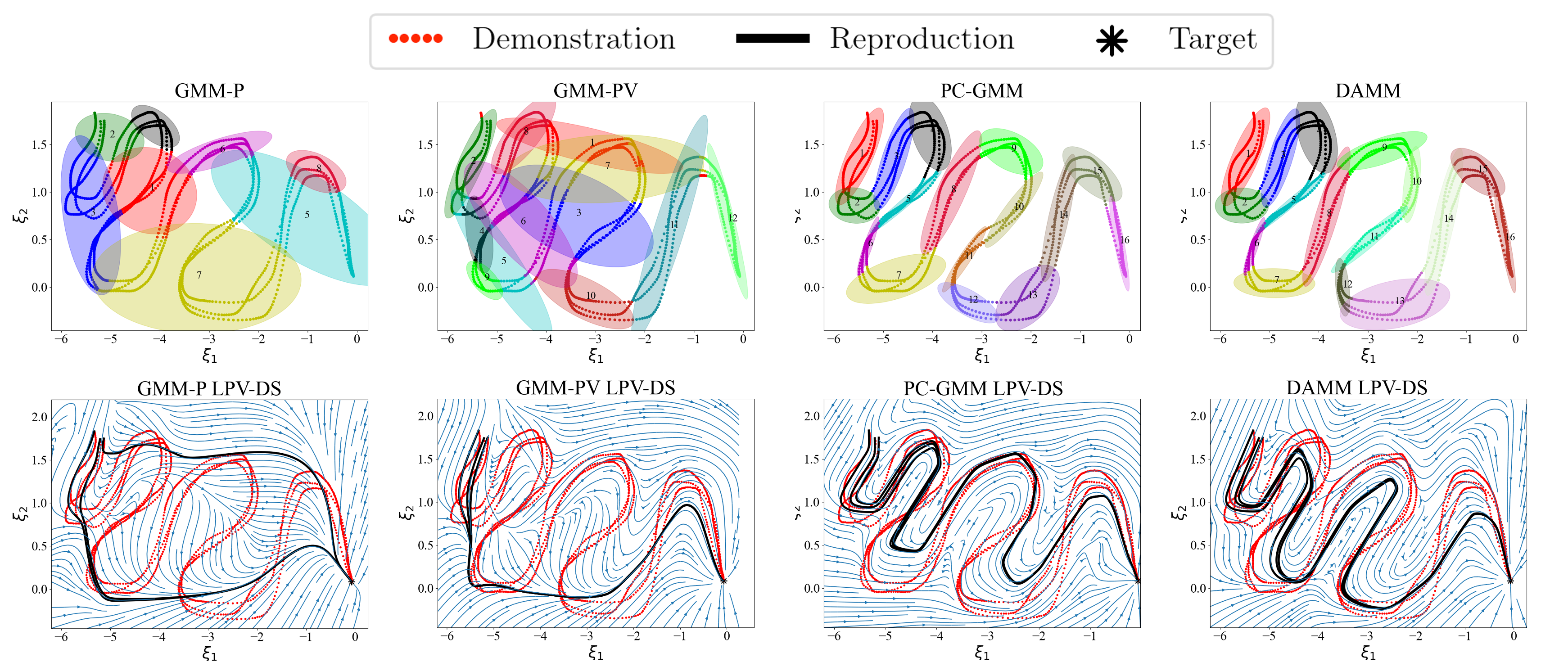
Figure 3: Comparison of clustering results (top) and LPV-DS results (bottom) between the GMM-P (position), GMM-PV (position+velocity), PC-GMM and DAMM on a messy snake trajectory [10]. The computation times are 0.2, 0.3, 55 and 1.8 in seconds from left to right. The number of components $K$ are 8, 12, 16 and 16 respectively.

Results: Table. I compares the performance between DAMM and baseline methods across the aforementioned metrics. Notably, the column of computation time shows that DAMM is comparable to vanilla GMM variants, and exhibits significant speedup to PC-GMM (our goal). We note that most of the computation expense in DAMM comes from the intermediate Gibbs sampling scans required to reach the launch state; however, DAMM is still able to complete a clustering task at an order of magnitude faster rate than PC-GMM thanks to being parallelizable. We further compare the completion speed between DAMM and baseline methods by investigating the computation time versus observation size. In Fig. 2, we show that when the task is to learn a trajectory of small size ($<500$ observations), the distinction in computation times are non-significant as all four methods can finish within 10 seconds. The distinction, however, becomes more pronounced when dealing with larger datasets. For example, given an average demonstration containing 7000 observations from LASA dataset, DAMM scales well with large datasets and completes the clustering task slightly beyond 10 seconds. On the contrary, the computation time of PC-GMM grows exponentially and it takes more than an hour to complete the task due to its strictly sequential nature.

The columns of BIC and AIC (lower the better) in Table. I show that DAMM outperforms the GMM variants in both the average and standard deviation. We further observe that when the trajectory is more linear, all methods are able to capture the meaningful motion and produce efficient clustering results. When the trajectory becomes non-linear, the results of GMM variants quickly deteriorate while DAMM is able to produce accurate probability distribution without compromising model complexity. As a result, more accurate probability models lead to producing better DS, and hence DAMM again outperforms the GMM baselines across all three metrics (lower the better) in the category of model accuracy. We further illustrate in Fig. 3 how the GMM variants on the first two columns from the left fail to capture the non-linearity of the messy-snake motion from the PC-GMM dataset; consequently producing erroneous dynamical systems. On the contrary, the last column in Fig. 3 shows that DAMM successfully segments the trajectory into linear portions and therefore results in a more accurate DS.

Comparing DAMM to PC-GMM in Table. I, DAMM exhibits a slight advantage in AIC and BIC. Although the difference between DAMM and PC-GMM is not statistically significant, DAMM remains comparable to the state-of-the-art in model efficiency yet superior in computational efficiency. In terms of model accuracy, DAMM holds a slight edge over PC-GMM in RMSE and DTWD. Once again, the non-significant difference is expected, as both DAMM and PC-GMM effectively capture directionality and generate appropriate models, leading to proper DS via optimization. Illustrations and code to reproduce the DAMM fitting and resulting LPV-DS vector fields for both LASA and PC-GMM benchmark datasets is available in our github code repository.

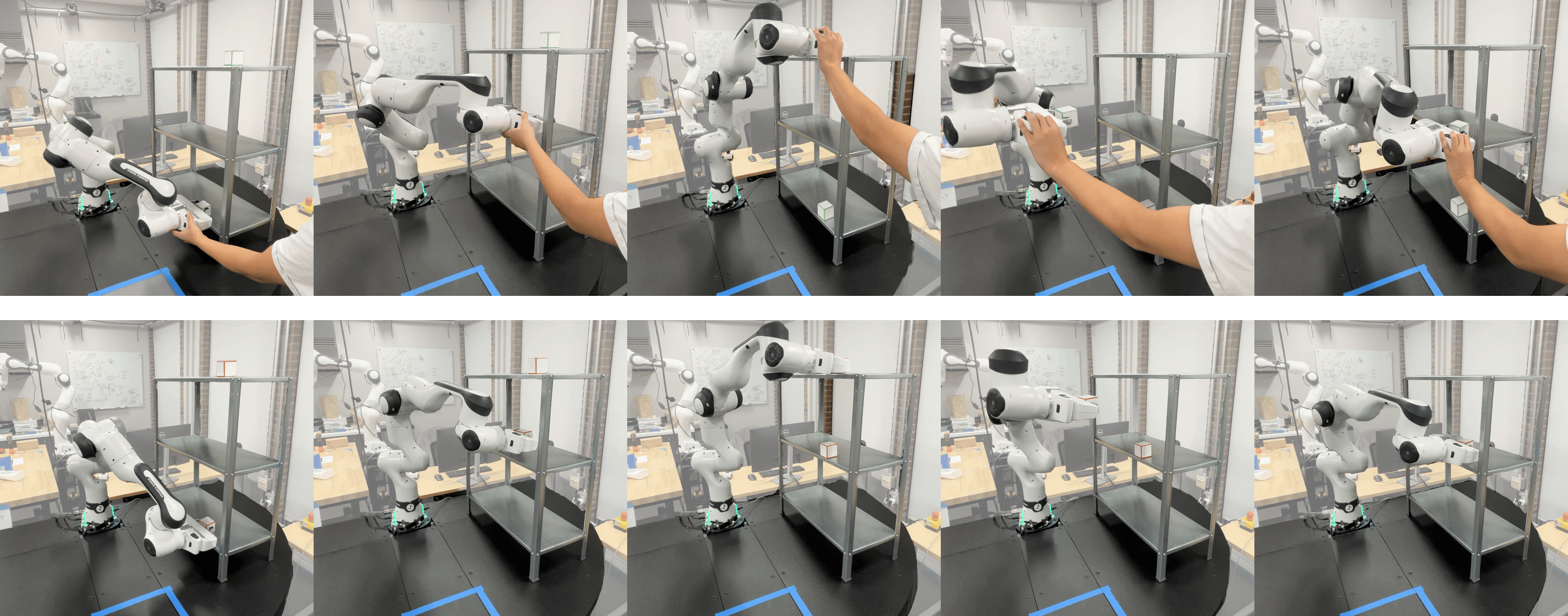
Figure 4: Snapshot sequences of a typical demonstration (top) and reproduction (bottom) of the bookshelf arrangement task. The computation time is 1.5 seconds. The number of components $K$ is 7.

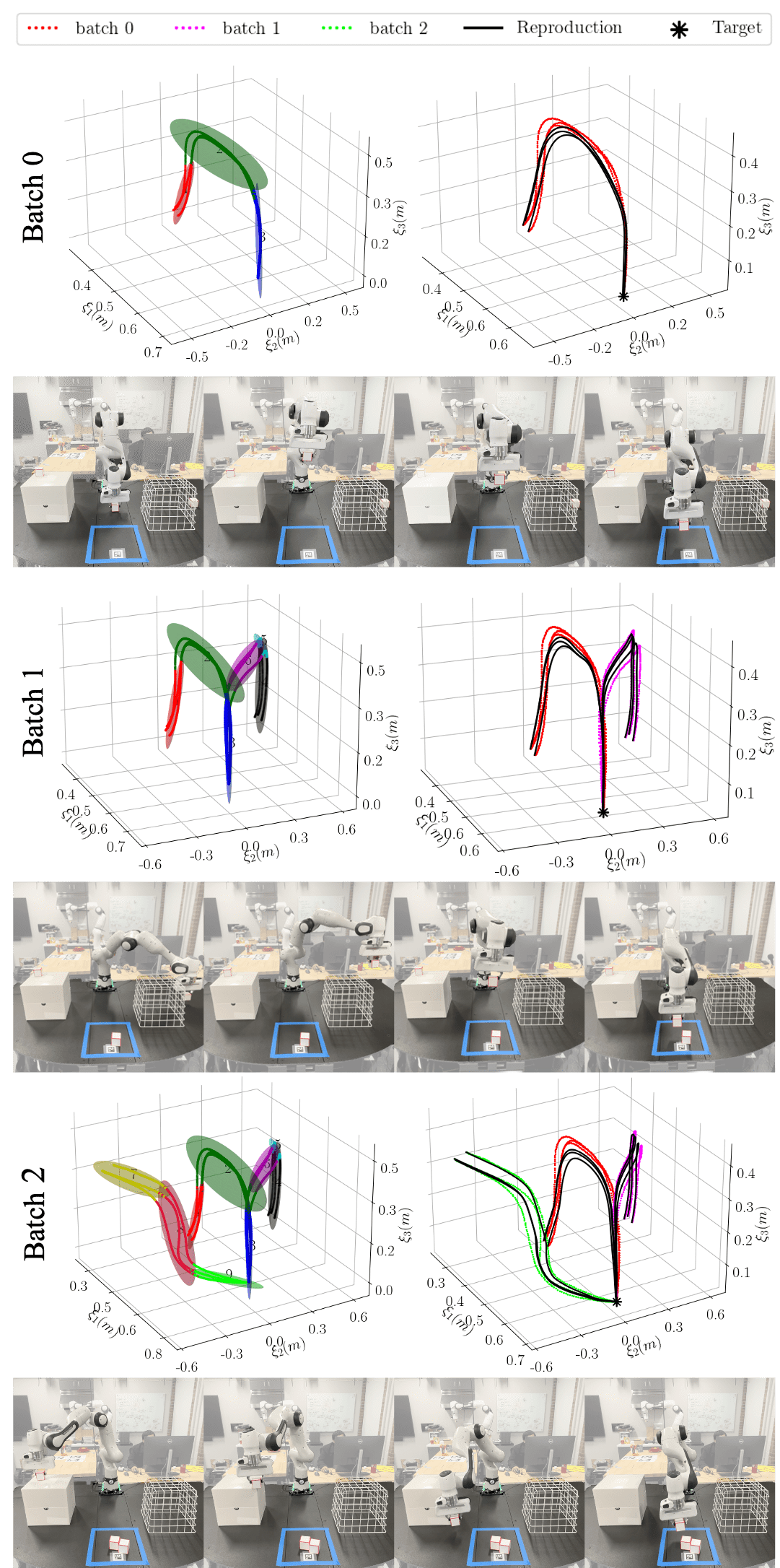
Figure 5: Sequence of learning three tasks incrementally via the DAMM-based LPV-DS. Every two rows correspond the learning of a new task with the clustering result (top left), the reproduction DS (top right), and the snapshot sequence of the execution (bottom). The computation times are 0.6, 0.5 and 0.5 in seconds respectively for each task. The total number of components $K$ after each task are 3, 6, and 9 respectively.

IV-C Robot Experiments

We validate DAMM on a Frank Emika robot through DS-based motion policies learned from demonstrations. In Fig. 4, we exemplify a typical bookshelf arrangement task containing 6 trajectories and 2500 observations. The top row illustrates that the demonstration was generated by humans guiding the robot to move the training objects from different initial locations (upper and lower shelves) to the target (middle shelf). The bottom row illustrates that the robot successfully executes the learned DS via DAMM-based LPV-DS, closely follows the demonstration trajectory and reaches the target as shown in the supplementary video.

IV-D Incremental Learning

In the setting of incremental learning where new data comes in progressively, the traditional approach is to concatenate batches and re-learn the combined trajectory, resulting in inefficient use of data. We therefore propose an alternative approach where new data can choose to either join existing components or form new groups while keeping the assignment of the previous batches unchanged. This efficiently reduces the task to clustering only the new data, circumventing the need to learn the combined batch.

In Fig. 5, we showcase the compatibility of DAMM in our new incremental learning framework where the robot sequentially learns three different tasks. Each task comprises 3 demonstrations and approximately 1500 observations. Upon receiving demonstration batch 0, the robot performs DAMM-based LPV-DS as usual with the clustering and the reproduction results shown in the first two rows of Fig. 5. Subsequently, we introduce another demonstration batch 1, which moves the object from different locations but later merges with batch 0. The middle two rows illustrate that the new demonstration initially forms distinct components but later joins the first demonstration as both batches converge. The reproduction DS and the snapshot sequence confirms the robot’s successful learning and execution of the new trajectory while preserving the preceding DS. When the last demonstration batch 2 comes in, with no overlapping with the previous batches, the last two rows show that batch 2 forms its own groups and the robot successfully executes the newly learned DS by moving the object to the target location via a different trajectory.

V Conclusion

We introduce the Directionality-Aware Mixture Model that is capable of effectively identifying the directional features of the trajectory data. By including both the positional and directional information using a proper Riemannian metric, DAMM produces physically-meaningful clustering results that represent the intrinsic structure of the trajectory data. Along with the parallel sampling scheme, the DAMM-based LPV-DS framework achieves a drastic improvement in computational efficiency while remaining comparable to the state-of-the-art level of model accuracy.

Appendix A Unit Sphere Manifold

Given $x,y\in\mathbb{S}^{d}$, the exponential and logarithmic maps are defined as:

$$y =\exp_{x}(u)=x\cos(\|u\|)+\frac{u}{\|u\|}\sin(\|u\|),$$ (16)

$$u =\log_{x}(y)=d(x,y)\frac{y-x^{T}yx}{\|y-x^{T}yx\|}$$ (17)

where the geodesic distance is $d(x,y)=\arccos(x^{T}y)$. Both $u$ and $v$ are vectors mapped in $T_{x}\mathbb{S}^{d}$.

Appendix B Merge Proposal

We define the launch state $\mathbf{z}^{l}$ by randomly initializing the assignments between two groups of interest and performing multiple scans of IW Gibbs sampler. We then compute the expressions below as if we are reaching the original split state from the $\mathbf{z}^{l}$ by one final scan of Gibbs sampler:

$$\dfrac{\pi(\mathbf{z}^{m})}{\pi(\mathbf{z})}=\dfrac{\displaystyle{\prod_{z_{i}=z^{m}_{12}}}\mathcal{N}(\hat{\xi}_{z_{i}}|\hat{\theta}_{z^{m}_{12}})}{\displaystyle{\prod_{z_{i}=z^{m}_{1}}}\pi_{1}\mathcal{N}(\hat{\xi}_{z_{i}}|\hat{\theta}_{z^{m}_{1}})\prod_{z_{i}=z^{m}_{2}}\pi_{2}\mathcal{N}(\hat{\xi}_{z_{i}}|\hat{\theta}_{z^{m}_{2}})}$$ (18)

$$\dfrac{q(\mathbf{z}|\mathbf{z}^{m})}{q(\mathbf{z}^{m}|\mathbf{z})}=\prod_{z_{i}=z^{l}_{1}}\prod_{z_{i}=z^{l}_{2}}\dfrac{\pi_{z_{i}}\mathcal{N}(\hat{\xi}_{z_{i}}|\hat{\theta}_{z_{i}})}{\pi_{z^{l}_{1}}\mathcal{N}(\hat{\xi}_{z_{i}}|\hat{\theta}_{z^{l}_{1}})+\pi_{z^{l}_{2}}\mathcal{N}(\hat{\xi}_{z_{i}}|\hat{\theta}_{z^{l}_{2}})}$$ (19)

where $z^{m}_{1}$ and $z^{m}_{2}$ are the respective assignment labels of the original components, and $z^{m}_{12}$ is the new assignment label of the combined component. $z^{l}_{1}$ and $z^{l}_{2}$ are the assignments of the two groups before the final scan of IW Gibbs sampler.

Appendix C LASA Dataset Benchmark

We evaluated our approach on the LASA handwriting dataset as outlined in Section. IV. We included the benchmark results in Fig. 6 and Fig. 7. Every three rows illustrate the results of five datasets, with the clustering results of DAMM(top), probability density function of the mixture model (middle), and reproduction DS (bottom).

Appendix D PC-GMM [10] Dataset Benchmark

We further illustrate the benchmark results of DAMM LPV-DS against other baseline methods on the PC-GMM benchmark dataset (2D and 3D real trajectories) [10]. We include 2D motions in Fig. 8, 9 and 10, and 3D motions in Fig. 11 and 12.

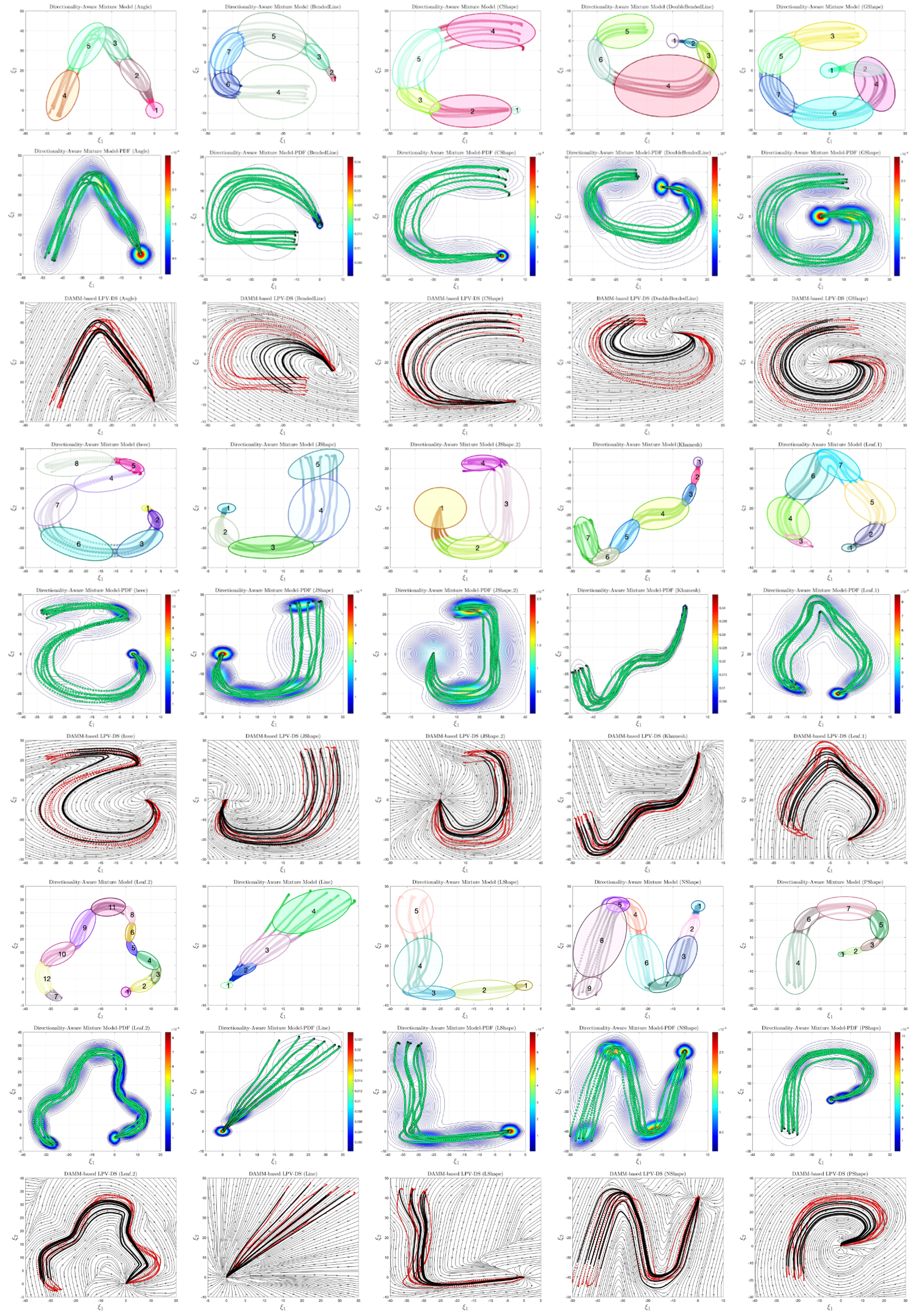
Figure 6: Results on the LASA Dataset with Learned Clusters and Reproduced Stream Graph using DAMM (Part 1).

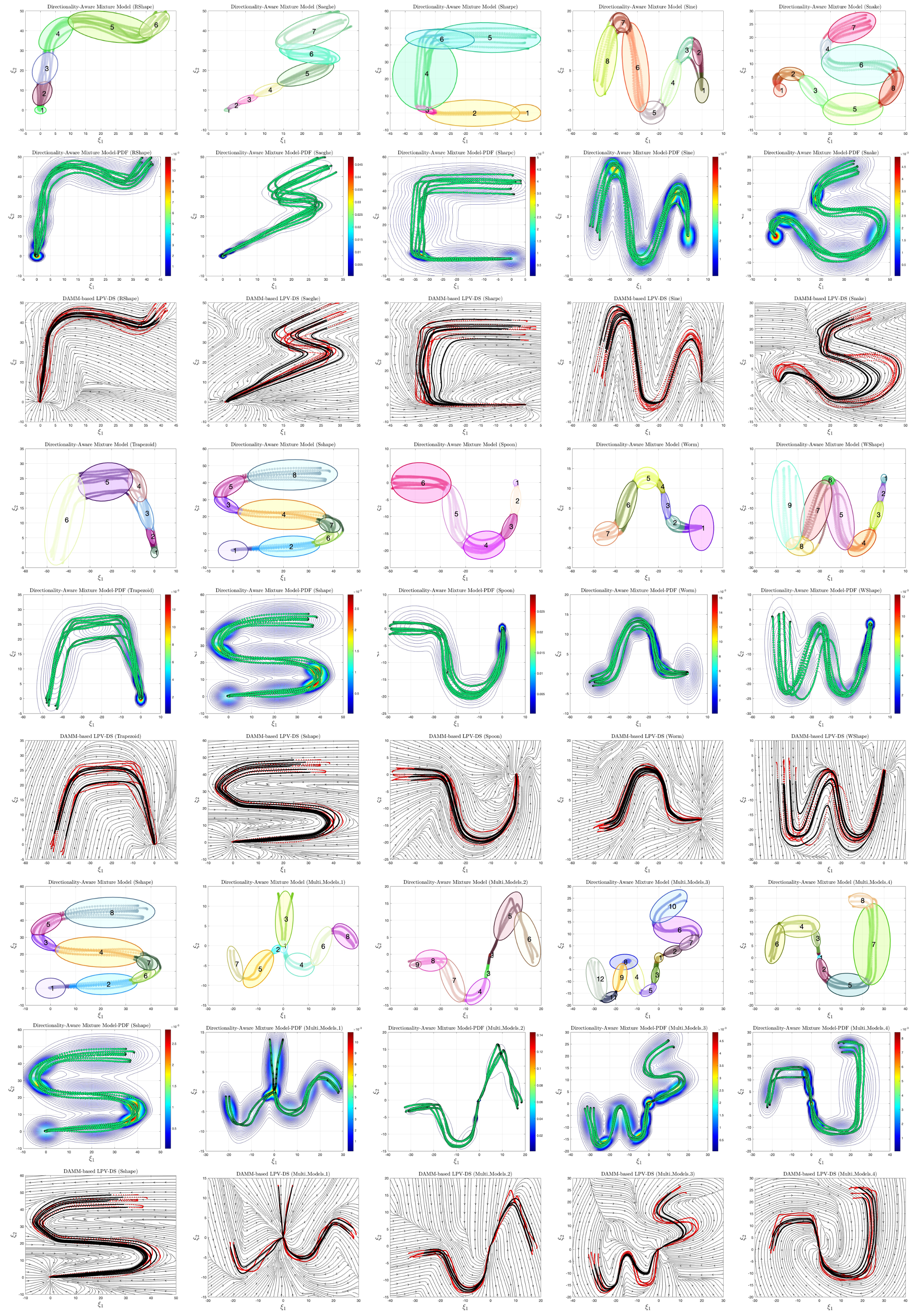
Figure 7: Results on the LASA Dataset with Learned Clusters and Reproduced Stream Graph using DAMM (Part 1).

Figure 8: Number of components: 8, 12, 16, 16. Computation time in seconds: 0.2, 0.3, 55, 1.8

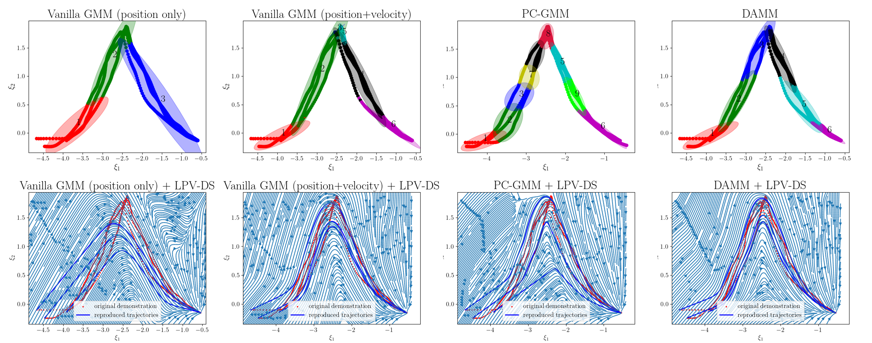
Figure 9: Number of components: 3, 6, 9, 6. Computation time in seconds: 3, 4, 47, 0.5

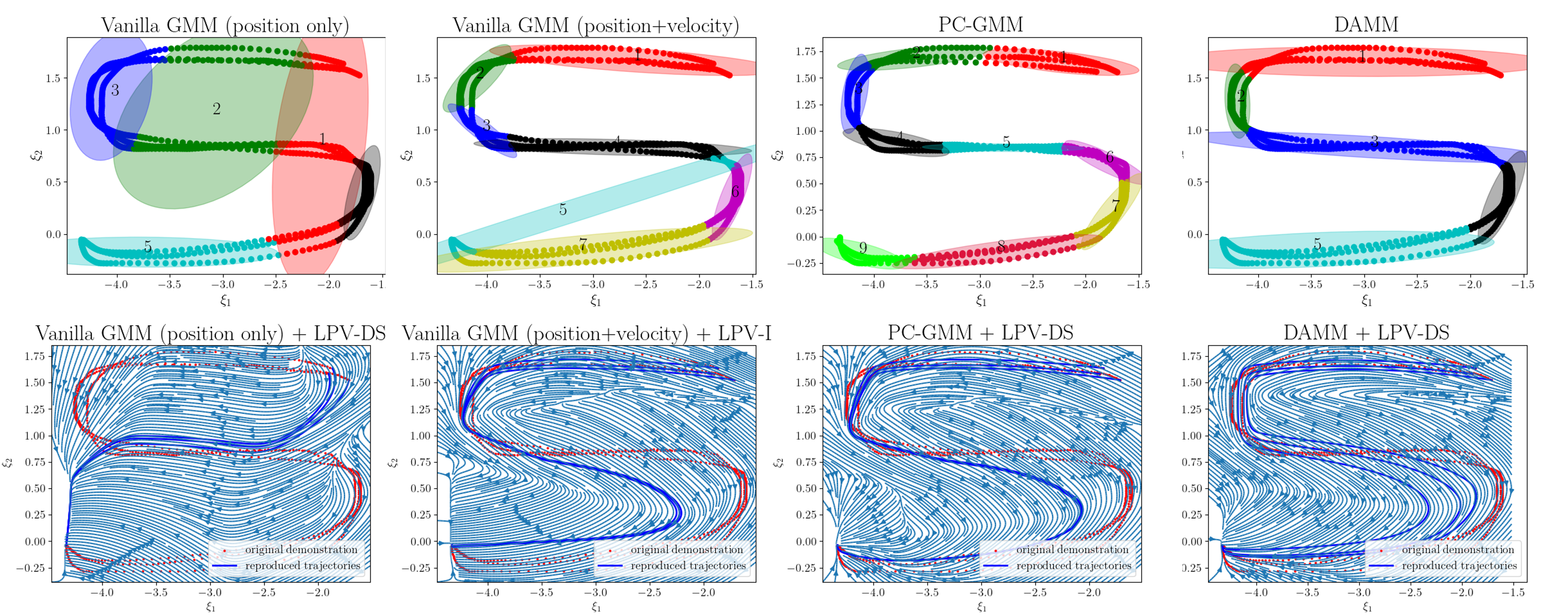
Figure 10: Number of components: 5, 7, 9, 5. Computation time in seconds: 0.5, 1, 60, 0.7

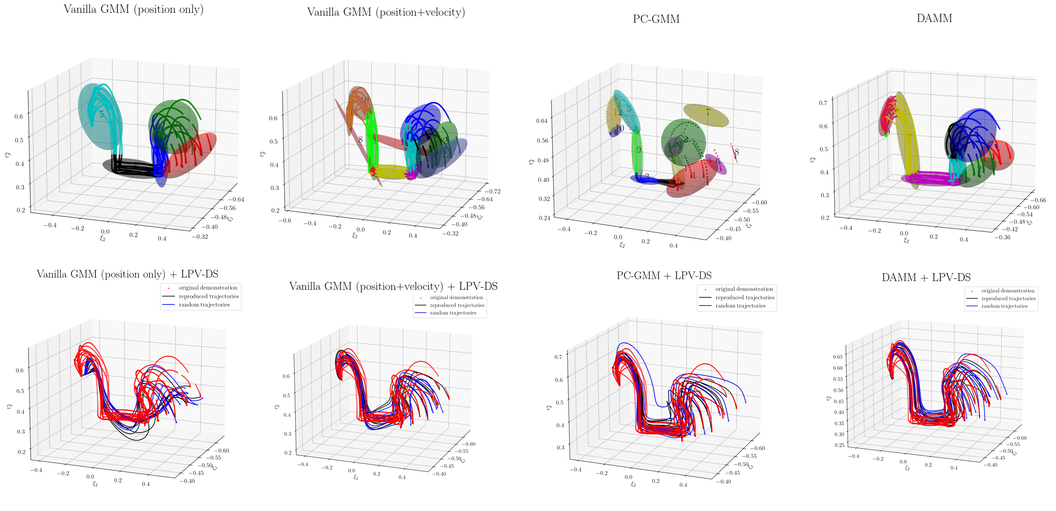
Figure 11: Number of components: 5, 10, 12, 9. computation time in seconds: 1.5, 2, 3700, 1.7

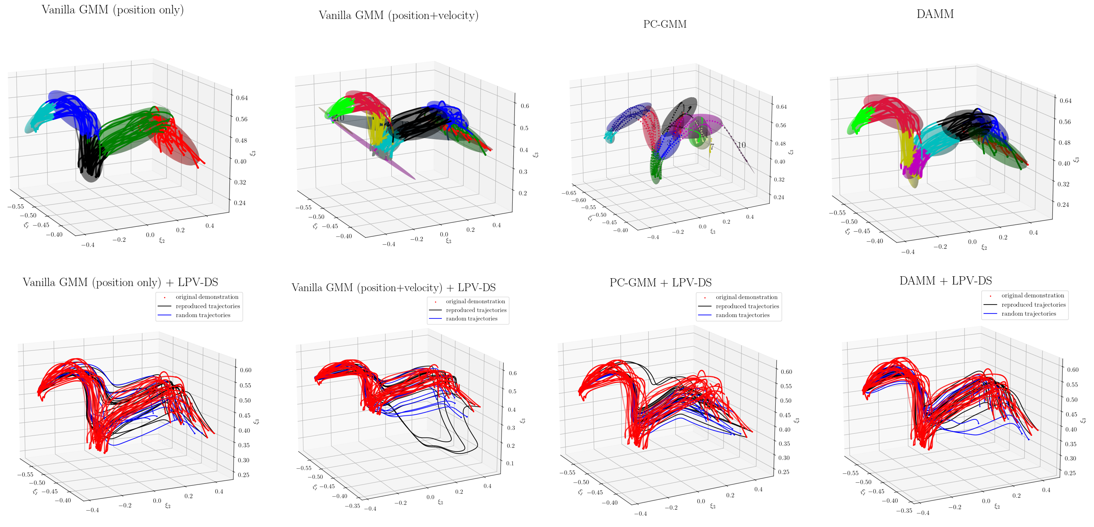
Figure 12: Number of components: 5, 11, 12, 9. computation time in seconds: 0.8, 1.2, 4200, 1.4

References

- [1] A. Ude, “Trajectory generation from noisy positions of object features for teaching robot paths,” Robotics and Autonomous Systems, vol. 11, no. 2, pp. 113–127, 1993.
- [2] J.-H. Hwang, R. Arkin, and D.-S. Kwon, “Mobile robots at your fingertip: Bezier curve on-line trajectory generation for supervisory control,” vol. 2, 11 2003, pp. 1444 – 1449 vol.2.
- [3] J. Aleotti and S. Caselli, “Robust trajectory learning and approximation for robot programming by demonstration,” Robotics and Autonomous Systems, vol. 54, no. 5, pp. 409–413, 2006.
- [4] A. Billard, S. Mirrazavi, and N. Figueroa, Learning for Adaptive and Reactive Robot Control: A Dynamical Systems Approach. The MIT Press, 2022.
- [5] E. Gribovskaya, S.-M. Khansari-Zadeh, and A. Billard, “Learning non-linear multivariate dynamics of motion in robotic manipulators,” IJRR, vol. 30, no. 1, pp. 80–117, 2011.
- [6] S. M. Khansari-Zadeh and A. Billard, “Learning stable non-linear dynamical systems with gaussian mixture models,” IEEE Transactions on Robotics, vol. 27, no. 5, pp. 943–957, 2011.
- [7] J. Urain, M. Ginesi, D. Tateo, and J. Peters, “Imitationflow: Learning deep stable stochastic dynamic systems by normalizing flows,” in 2020 IEEE/RSJ IROS, 2020, pp. 5231–5237.
- [8] M. A. Rana, A. Li, D. Fox, B. Boots, F. Ramos, and N. Ratliff, “Euclideanizing flows: Diffeomorphic reduction for learning stable dynamical systems,” in Proc. of the 2nd Conference on Learning for Dynamics and Control, vol. 120. PMLR, Jun 2020, pp. 630–639.
- [9] R. Pérez-Dattari and J. Kober, “Stable motion primitives via imitation and contrastive learning,” IEEE Transactions on Robotics, vol. 39, no. 5, pp. 3909–3928, 2023.
- [10] N. Figueroa and A. Billard, “A physically-consistent bayesian non-parametric mixture model for dynamical system learning,” in Proc. of The 2nd Conference on Robot Learning, vol. 87. PMLR, 2018, pp. 927–948.
- [11] J. Straub, J. Chang, O. Freifeld, and J. Fisher III, “A Dirichlet Process Mixture Model for Spherical Data,” in Proceedings of the Eighteenth International Conference on Artificial Intelligence and Statistics, ser. Proceedings of Machine Learning Research, vol. 38. PMLR, 09–12 May 2015, pp. 930–938.
- [12] S. M. Khansari-Zadeh and A. Billard, “Learning control lyapunov function to ensure stability of dynamical system-based robot reaching motions,” Robotics and Autonomous Systems, vol. 62, no. 6, pp. 752–765, 2014.
- [13] H. K. Khalil, Nonlinear systems; 3rd ed. Upper Saddle River, NJ: Prentice-Hall, 2002, the book can be consulted by contacting: PH-AID: Wallet, Lionel. [Online]. Available: https://cds.cern.ch/record/1173048
- [14] D. Blei and P. Frazier, “Distance dependent chinese restaurant processes,” Journal of Machine Learning Research, vol. 12, pp. 2461–2488, 08 2011.
- [15] M. do Carmo, Riemannian Geometry, ser. Mathematics (Boston, Mass.). Birkhäuser, 1992.
- [16] J. Lee, Introduction to Riemannian Manifolds, ser. Graduate Texts in Mathematics. Springer International Publishing, 2019.
- [17] M. Arnaudon, F. Barbaresco, and L. Yang, “Medians and means in riemannian geometry: Existence, uniqueness and computation,” 11 2011.
- [18] X. Pennec, “Intrinsic statistics on riemannian manifolds: Basic tools for geometric measurements,” Journal of Mathematical Imaging and Vision, vol. 25, pp. 127–154, 07 2006.
- [19] M. J. A. Zeestraten, I. Havoutis, J. Silvério, S. Calinon, and D. G. Caldwell, “An approach for imitation learning on riemannian manifolds,” IEEE RA-L, vol. 2, no. 3, pp. 1240–1247, 2017.
- [20] S. Calinon, “Gaussians on riemannian manifolds: Applications for robot learning and adaptive control,” IEEE Robotics & Automation Magazine, vol. 27, no. 2, pp. 33–45, 2020.
- [21] J. Sethuraman, “A constructive definition of dirichlet priors,” Statistica Sinica, vol. 4, no. 2, pp. 639–650, 1994.
- [22] K. P. Murphy, “Conjugate bayesian analysis of the Gaussian distribution,” 2007.
- [23] R. M. Neal, “Markov chain sampling methods for dirichlet process mixture models,” Journal of Computational and Graphical Statistics, vol. 9, no. 2, pp. 249–265, 2000.
- [24] J. Chang and J. W. Fisher III, “Parallel sampling of DP mixture models using sub-cluster splits,” in Advances in Neural Information Processing Systems, vol. 26, 2013.
- [25] S. Jain and R. M. Neal, “A split-merge markov chain monte carlo procedure for the dirichlet process mixture model,” Journal of Computational and Graphical Statistics, vol. 13, no. 1, pp. 158–182, 2004.
- [26] N. Metropolis, A. W. Rosenbluth, M. N. Rosenbluth, A. H. Teller, and E. Teller, “Equation of state calculations by fast computing machines,” 3 1953.
- [27] W. K. Hastings, “Monte carlo sampling methods using markov chains and their applications,” Biometrika, vol. 57, no. 1, pp. 97–109, 1970.
- [28] J. R. Medina and A. Billard, “Learning stable task sequences from demonstration with linear parameter varying systems and hidden markov models,” in Proceedings of the 1st Annual Conference on Robot Learning, vol. 78. PMLR, 13–15 Nov 2017, pp. 175–184.