BEVTrack: A Simple and Strong Baseline for 3D Single Object Tracking in Bird’s-Eye View

Abstract

3D Single Object Tracking (SOT) is a fundamental task of computer vision, proving essential for applications like autonomous driving. It remains challenging to localize the target from surroundings due to appearance variations, distractors, and the high sparsity of point clouds. The spatial information indicating objects’ spatial adjacency across consecutive frames is crucial for effective object tracking. However, existing trackers typically employ point-wise representation with irregular formats, leading to insufficient use of this important spatial knowledge. As a result, these trackers usually require elaborate designs and solving multiple subtasks. In this paper, we propose BEVTrack, a simple yet effective baseline that performs tracking in Bird’s-Eye View (BEV). This representation greatly retains spatial information owing to its ordered structure and inherently encodes the implicit motion relations of the target as well as distractors. To achieve accurate regression for targets with diverse attributes (e.g., sizes and motion patterns), BEVTrack constructs the likelihood function with the learned underlying distributions adapted to different targets, rather than making a fixed Laplace or Gaussian assumption as in previous works. This provides valuable priors for tracking and thus further boosts performance. While only using a single regression loss with a plain convolutional architecture, BEVTrack achieves state-of-the-art performance on three large-scale datasets, KITTI, NuScenes, and Waymo Open Dataset while maintaining a high inference speed of about 200 FPS. The code will be released at BEVTrack.

I Introduction

3D single object tracking (SOT) is crucial for various applications, such as autonomous driving [1, 2, 3]. It aims to localize a specific target across a sequence of point clouds, given only its initial status. Existing tracking approaches [4, 5] commonly adopt the point-wise representation, directly taking raw point clouds as input. For example, P2B[4] and its follow-up works [6, 7, 8] adopt a point-based network [9, 10] with the Siamese architecture for feature extraction, followed by a point-wise appearance matching module [4, 8, 11] for propagation of target cues, and a 3D Region Proposal Network [12, 13] for target localization, as illustrated in Fig. 1(a). M2-Track[5] proposes a motion-centric paradigm, that first segments the target points from their surroundings with a PointNet [14] segmentation network and then localizes the target through a motion modeling approach followed by a box refinement module, as illustrated in Fig. 1(b).

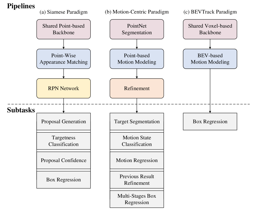
Figure 1: Comparison with typical 3D SOT paradigms. Previous methods mainly rely on the point-wise representation, and decompose the tracking problem into multiple subtasks, leading to a complicated tracking framework. On the contrary, our proposed BEVTrack performs tracking in BEV, greatly retaining the spatial information and thus simplifying the tracking pipeline while improving the performance.

Although these approaches have exhibited superior performance in tracking benchmarks, they usually require elaborate designs [11, 15, 8, 16] and solving multiple subtasks [5, 4] to establish target correspondences across consecutive frames, resulting in complicated tracking frameworks and challenges in hyper-parameter tuning. It is noteworthy that such correspondences naturally exist as objects exhibit continuous motion within the video sequence [17, 18]. This spatial continuity offers valuable prior knowledge for target localization, whereas the point-wise representation [14, 9] with irregular formats fails to utilize it.

In this paper, we present BEVTrack, a simple yet strong baseline for 3D SOT, as shown in Fig. 1(c). Converting unordered point clouds into the BEV representation [19, 20, 21], BEVTrack greatly exploits spatial information and inherently encodes the implicit motion relations of the target as well as distractors in BEV. Specifically, we first adopt a voxel-based network [19] with the Siamese architecture for feature extraction. Subsequently, we squeeze the sparse 3D features along the height dimension to obtain the BEV features. Given that corresponding objects are spatially adjacent in the BEV features across consecutive frames, we can easily fuse them together with an element-wise operation such as concatenation. Thanks to the utilization of spatial information, we can intuitively model the motion cues of the target as well as distractors in BEV via a simple convolutional structure, which is beneficial for identifying the target and accurate localization, especially in challenging scenarios. Finally, we discard the complicated region proposal network while using a global max pooling followed by a lightweight multilayer perceptron (MLP) to localize the target, resulting in a simple one-stage tracking pipeline with a single regression loss.

To optimize the regression-based trackers, current approaches typically employ conventional $L_{1}$ or $L_{2}$ loss. This kind of supervision actually makes a fixed Laplace or Gaussian assumption on the data distribution, which is inflexible when handling targets possessing diverse attributes (e.g., sizes, moving patterns, and sparsity degrees). For example, when tracking targets with high sparsity degrees, where the predictions may be uncertain while the annotations are not very reliable, the outputs should conform to a distribution with a large variance. To this end, we introduce a novel distribution-aware regression strategy for tracking, which constructs the likelihood function with the learned underlying distributions adapted to distinct targets, instead of making a fixed assumption. Note that this strategy does not participate in the inference phase, thus boosting the tracking performance without additional computation overhead. Despite no elaborate design, BEVTrack exhibits a substantial performance advantage over the current state-of-the-art (SOTA) methods on challenging tracking datasets, i.e., KITTI [22], NuScenes [23], and Waymo Open Dataset [24], while running at real-time (about 200 FPS).

The main contributions of this paper are three-fold:

$\bullet$ We propose BEVTrack, a simple yet strong baseline for 3D SOT. This pioneering approach efficiently leverages spatial information in BEV, resulting in a simplified tracking pipeline design.

$\bullet$ We present a novel distribution-aware regression strategy for tracking, which constructs the likelihood function with the learned underlying distributions adapted to targets possessing diverse attributes. This strategy provides accurate guidance for tracking, resulting in improved performance while avoiding extra computation overhead.

$\bullet$ BEVTrack achieves SOTA performance on three popular benchmarks while maintaining a high inference speed.

II Related Work

II-A 3D Single Object Tracking

Early 3D SOT approaches [25, 26] predominantly utilize RGB-D data and often adapt 2D Siamese networks [27, 28, 29, 30] by integrating depth maps. However, variations in illumination and appearance can adversely affect the performance of such RGB-D techniques. SC3D [31] is the first 3D Siamese tracker based on shape completion that generates a large number of candidates in the search area and compares them with the cropped template, taking the most similar candidate as the tracking result. The pipeline relies on heuristic sampling and does not learn end-to-end, which is very time-consuming.

To address these issues, P2B [4] develops an end-to-end framework by employing a shared point-based backbone for feature extraction, followed by a point-wise appearance-matching technique for target cues propagation. Ultimately, a Region Proposal Network is used to derive 3D proposals, of which the one with the peak score is selected as the final output. P2B reaches a balance between performance and efficiency, and many works [6, 32, 8, 15, 33] follow the same paradigm. Drawing inspiration from the success of transformers [34], many studies have incorporated elaborate attention mechanisms to enhance feature extraction and target-specific propagation. For instance, PTT [32] introduces the Point Track Transformer to enhance point features. PTTR [8] presents the Point Relation Transformer for target-specific propagation and a Prediction Refinement Module for precision localization. Similarly, ST-Net [15] puts forth an iterative correlation network, and CXTrack [11] presents the Target Centric Transformer to harness contextual information from consecutive frames. Unlike the Siamese paradigm, M2-Track [5] proposes a motion-centric paradigm, explicitly modeling the target’s motion between two successive frames.

Despite achieving promising results on popular datasets, these trackers necessitate elaborate designs and solving multiple subtasks, as they typically rely on point-wise representation that hinders the efficient utilization of spatial information. Albeit V2B [35] recommends converting the enhanced point features into dense BEV feature maps to generate high-quality target proposals, it retains using the point-wise representation for target cues propagation. In contrast, our method adopts the BEV representation that facilitates utilizing spatial information and inherently encodes the implicit motion relations of the target as well as distractors, thus achieving superior performance while only using a single regression loss with a plain convolutional architecture.

II-B BEV Representation for LiDAR-based Perception

Some approaches have been proposed to directly process point cloud data [14, 9, 12] with the inter-point neighborhood relationship computed in continuous 3D space. However, they bring more computational overhead, while restricting the neural network’s receptive field, thus hindering spatial information utilization. Recently, learning powerful BEV representations [36] for perception tasks is drawing extensive attention both from industry and academia. There are mainly two branches to convert point cloud data into BEV representation: 1) Pre-BEV [19, 37, 38], which extracts point cloud features in 3D space and usually achieves accurate results, and 2) Post-BEV [20, 39], which extracts BEV features in 2D space directly and is more computationally efficient. BEVTrack follows the Pre-BEV paradigm that utilizes voxels with fine-grained size, preserving most of the 3D information from point cloud data and thus achieving accurate tracking results.

III Method

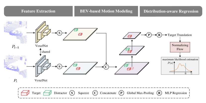
Figure 2: Architecture of BEVTrack. The proposed framework contains three parts including voxel-based feature extraction, BEV-based motion modeling, and distribution-aware regression. Our BEVTrack is a simple tracking baseline framework with a plain convolutional architecture and a single regression loss, yet demonstrating state-of-the-art performance.

III-A Overview

Given the 3D bounding box (BBox) of a specific target at the initial frame, 3D SOT aims to localize the target by predicting its 3D BBoxes in the subsequent frames. A 3D BBox $\mathcal{B}_{t}\in\mathbb{R}^{7}$ is parameterized by its center (i.e., $x,y,z$ coordinates), orientation (i.e., heading angle $\theta$ around the $up$-axis), and size (i.e., width, length, and height). Suppose the point clouds in two consecutive frames are denoted as $\mathcal{P}_{t-1}\in\mathbb{R}^{N_{t-1}\times 3}$ and $\mathcal{P}_{t}\in\mathbb{R}^{N_{t}\times 3}$, respectively, where $N_{t-1}$ and $N_{t}$ are the numbers of points in the point clouds. At timestamp $t$, we take all points of $\mathcal{P}_{t-1}$ and $\mathcal{P}_{t}$ within the search region as input, leveraging complete contextual information [11] around the targets without cropping or sampling to handle appearance variations and targets occlusion. Since the tracking target has a small change in size and orientation, we assume constant target size and orientation, and only regress the inter-frame target translation offsets (i.e., $\Delta x,\Delta y,\Delta z$) to simplify the tracking task. By applying the translation to the 3D BBox $\mathcal{B}_{t-1}$, we can compute the 3D BBox $\mathcal{B}_{t}$ to localize the target in the current frame. The tracking process can be formulated as:

$$\mathcal{F(P_{\mathit{t-1}},P_{\mathit{t}})}\mapsto(\Delta x,\Delta y,\Delta z),$$ (1)

where $\mathcal{F}$ is the mapping function learned by the tracker.

Following Eq. (1), we propose BEVTrack, a simple yet strong baseline for 3D SOT. The overall architecture of BEVTrack is presented in Fig. 2. It first employs a shared voxel-based backbone [19] to extract 3D features, which are then squeezed to derive the BEV features (Sec. III-B). Subsequently, BEVTrack fuses the BEV features via a concatenation operation and several convolutional layers (Sec. III-C). Finally, it adopts a simple prediction head which contains a global max pooling layer followed by a lightweight MLP. For accurate regression, we optimize the model with a novel distribution-aware regression strategy in the training phase (Sec. III-D).

III-B Feature Extraction

To localize the target from surroundings accurately, we need to learn discriminative features from the point clouds. Instead of using a point-based backbone [14, 9, 10] as in [4, 5, 11], we adopt a variant of VoxelNet [19] as the shared backbone, which modifies the original architecture by removing residual connections, utilizing sparse 3D convolutions [40, 41], and choosing suitable network hyper-parameters, such as voxel size. Specifically, we voxelize the 3D space into regular voxels and extract the voxel-wise features of each non-empty voxel by a stack of sparse convolutions, where the initial feature of each voxel is simply calculated as the mean values of point coordinates within each voxel in the canonical coordinate system. The spatial resolution is downsampled 8 times by three sparse convolutions of stride 2, each of which is followed by several submanifold sparse convolutions [40]. Afterwards, we squeeze the sparse 3D features along the height dimension to derive the BEV features $\mathcal{B}_{t-1}\in\mathbb{R}^{H\times W\times C}$ and $\mathcal{B}_{t}\in\mathbb{R}^{H\times W\times C}$, where $H$ and $W$ denote the 2D grid dimension and $C$ is the number of feature channels.

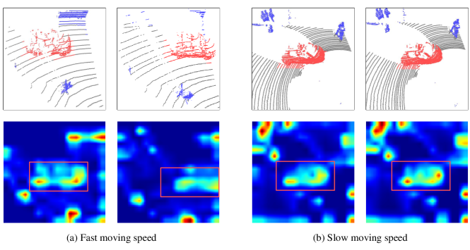
Figure 3: The motion pattern of objects is variable in different scenes. The top rows show point cloud scenes across two consecutive frames, where the red points indicate the target. The bottom rows visualize the heatmaps of the BEV response map with ground-truth bounding box (in red rectangles).

III-C BEV-based Motion Modeling

BEV-based Motion Modeling (BMM) aims to model the motion relations of the target as well as distractors in BEV, while propagating the target cues from the previous frame to the current frame. Given the BEV features $\mathcal{B}_{t-1}$ and $\mathcal{B}_{t}$, the corresponding objects are spatially adjacent across them. Therefore, we can easily fuse them together with an element-wise operator such as concatenation to preserve their spatial proximity. Furthermore, we apply several convolutional blocks to encode their motion relations. It is noteworthy that the receptive field of the convolution is limited due to the small kernel size, while the motion pattern of objects is variable in different scenes. As shown in Fig. 3, objects with a fast-moving speed are far apart across the BEV feature maps. To deal with this issue, we propose to enlarge the receptive field through spatial down-sampling by inserting convolutions of stride 2 at intervals, allowing it to capture a wide range of motion patterns. The above process can be formulated as:

$$\mathcal{F}=\text{Conv}([\mathcal{B}_{t-1};\mathcal{B}_{t}]),$$ (2)

where Conv denotes the convolutional blocks in BMM and $[;]$ denotes the concatenation operator. $\mathcal{F}\in\mathbb{R}^{H^{\prime}\times W^{\prime}\times C^{\prime}}$, where $H^{\prime}$, $W^{\prime}$, and $C^{\prime}$ denote the spatial dimension and the number of feature channels, respectively.

III-D Distribution-aware Regression

Different from the existing two-stage point-to-box prediction head [4, 8, 15], which contains two parts of proposals generation and proposal-wise scores prediction, we propose a one-stage post-processing-free prediction head consisting of only a global max-pooling layer and an MLP, i.e.,

$$\mathcal{C}=\text{MLP}(\text{Pool}(\mathcal{F})),$$ (3)

where $\mathcal{C}\in\mathbb{R}^{6}$ denotes the expectation of the target translation offsets $\bar{u}\in\mathbb{R}^{3}$ and the standard deviation $\sigma\in\mathbb{R}^{3}$, in contrast to prior methods that solely regress the deterministic target motion $u$. By applying the predicted translation to the last state of the target, we can localize the target in the current frame. Note that the standard deviation $\sigma$ enables dynamic optimization during training while being removed in the inference phase, as elaborated below.

The difference in sizes, moving patterns, and sparsity degrees among the tracked targets poses great challenges to existing trackers. To address this issue, we propose a novel distribution-aware regression strategy for tracking, which constructs the likelihood function with the learned underlying distributions adapted to distinct targets. In this way, the model can adaptively handle targets with different attributes, thus improving tracking performance.

Following [42], we model the distribution of the target motion $u\sim P(u)$ with reparameterization, which assumes that objects belonging to the same category share the same density function family, but with different mean and variance. Specifically, $P(u)$ can be obtained by scaling and shifting $z$ from a zero-mean distribution $z\sim P_{Z}(z)$ with transformation function $u=\bar{u}+\sigma\cdot z$, where $\bar{u}$ denotes the expectation of the target translation offsets and $\sigma$ denotes the scale factor of the distribution. $P_{Z}(z)$ can be modeled by a normalizing flow model (e.g., real NVP [43]). Given this transformation function, the density function of $P(u)$ can be calculated as:

$$\log P(u)=\log P_{Z}(z)-\log\sigma.$$ (4)

In this work, we employ residual log-likelihood estimation in [42] to estimate the above parameters, which factorizes the distribution $P_{Z}(z)$ into one prior distribution $Q_{Z}(z)$ (e.g., Laplace distribution or Gaussian distribution) and one learned distribution $G_{Z}(z\mid\theta)$. To maximize the likelihood in Eq. (4), we can minimize the following loss:

$$\mathcal{L}=-\log Q_{Z}(\hat{z})-\log G_{Z}(\hat{z}\mid\theta)+\log\sigma.$$ (5)

Here, $\hat{z}=(\hat{u}-\bar{u})/\sigma$, $\hat{u}$ is the ground truth translation offsets.

TABLE I: Comparisons with state-of-the-art methods on KITTI dataset. Success/Precision are used for evaluation. Bold and underline denote the best and the second-best scores, respectively.

Method	Car (6424)	Pedestrian (6088)	Van (1248)	Cyclist (308)	Mean by Class	Mean (14068)
SC3D	41.3 / 57.9	18.2 / 37.8	40.4 / 47.0	41.5 / 70.4	35.4 / 53.3	31.2 / 48.5
P2B	56.2 / 72.8	28.7 / 49.6	40.8 / 48.4	32.1 / 44.7	39.5 / 53.9	42.4 / 60.0
3DSiamRPN	58.2 / 76.2	35.2 / 56.2	45.7 / 52.9	36.2 / 49.0	43.8 / 58.6	46.7 / 64.9
BAT	60.5 / 77.7	42.1 / 70.1	52.4 / 67.0	33.7 / 45.4	47.2 / 65.1	51.2 / 72.8
PTT	67.8 / 81.8	44.9 / 72.0	43.6 / 52.5	37.2 / 47.3	48.4 / 63.4	55.1 / 74.2
V2B	70.5 / 81.3	48.3 / 73.5	50.1 / 58.0	40.8 / 49.7	52.4 / 65.6	58.4 / 75.2
PTTR	65.2 / 77.4	50.9 / 81.6	52.5 / 61.8	65.1 / 90.5	58.4 / 77.8	57.9 / 78.1
GLT-T	68.2 / 82.1	52.4 / 78.8	52.6 / 62.9	68.9 / 92.1	60.5 / 79.0	60.1 / 79.3
OSP2B	67.5 / 82.3	53.6 / 85.1	56.3 / 66.2	65.6 / 90.5	60.8 / 81.0	60.5 / 82.3
STNet	72.1 / 84.0	49.9 / 77.2	58.0 / 70.6	73.5 / 93.7	63.4 / 81.4	61.3 / 80.1
M2-Track	65.5 / 80.8	61.5 / 88.2	53.8 / 70.7	73.2 / 93.5	63.5 / 83.3	62.9 / 83.4
CXTrack	69.1 / 81.6	67.0 / 91.5	60.0 / 71.8	74.2 / 94.3	67.6 / 84.8	67.5 / 85.3
BEVTrack	71.7 / 84.1	68.4 / 92.7	65.7 / 76.2	74.6 / 94.7	70.1 / 86.9	69.8 / 87.4
Improvement	↓0.4 / ↑0.1	↑1.4 / ↑1.2	↑5.7 / ↑4.4	↑0.4 / ↑0.4	↑2.5 / ↑2.1	↑2.3 / ↑2.1

III-E Implementation Details

Different from previous works that choose the search region by enlarging the template BBox by 2 meters, the voxel-based backbone requires a fixed search region. In our experiments, we use a point cloud range of [(-4.8, 4.8), (-4.8, 4.8), (-1.5, 1.5)] meters and a voxel size of [0.075, 0.075, 0.15] meters for Car and Van. For non-rigid objects including Pedestrian and Cyclist, we adopt a range of [(-1.92, 1.92), (-1.92, 1.92), (-1.5, 1.5)] meters and a voxel size of [0.03, 0.03, 0.15] meters. For large objects such as Truck, Trailer, and Bus, we adopt a range of [(-9.6, 9.6), (-9.6, 9.6), (-3.0, 3.0)] meters and a voxel size of [0.15, 0.15, 0.3] meters. We use all points within the search region as input for both consecutive frames, without cropping and sampling.

We use 4 sparse convolution blocks with {16, 32, 64, 128} channels as the Siamese backbone. In our paper, we adopt RealNVP [43] to learn the underlying residual log-likelihood. The RealNVP model is fast and lightweight. We adopt 3 blocks with 64 channels for the RealNVP design, while each block consists of 3 fully connected (FC) layers and each FC layer is followed by a Leaky-RELU[44] layer.

Our BEVTrack can be trained in an end-to-end manner. We train it on 2 NVIDIA GTX 4090 GPUs for 160 epochs using the AdamW optimizer with a learning rate of 1e-4. We use a batch size of 256 and a weight decay of 1e-5. For data augmentations, we adopt common schemes including random flipping, random rotation, and random translation during the training. The loss function is a single regression loss.

IV Experiment

IV-A Experimental Settings

Datasets.

We validate the effectiveness of BEVTrack on three widely-used challenging datasets: KITTI [22], NuScenes [23], and Waymo Open Dataset (WOD) [24]. KITTI contains 21 video sequences for training and 29 video sequences for testing. We follow previous work [4] to split the training set into train/val/test splits due to the inaccessibility of the labels of the test set. NuScenes contains 1,000 scenes, which are divided into 700/150/150 scenes for train/val/test. Following the implementation in [6], we compare with the previous methods on five categories including Car, Pedestrian, Truck, Trailer, and Bus. For WOD, we follow LiDAR-SOT [45] to evaluate our method on 1,121 tracklets, which are split into easy, medium, and hard subsets according to the number of points in the first frame of each tracklet. Following ST-Net [15], we use the trained model on the KITTI dataset for evaluation on the WOD to assess the generalization ability of our 3D tracker.

Evaluation Metrics.

Following [4], we adopt Success and Precision defined in one pass evaluation (OPE) [46] as the evaluation metrics. Success denotes the Area Under Curve (AUC) for the plot showing the ratio of frames where the Intersection Over Union (IoU) between the predicted box and the ground truth is larger than a threshold, ranging from 0 to 1, while Precision denotes the AUC for the plot showing the ratio of frames where the distance between their centers is within a threshold, ranging from 0 to 2 meters.

IV-B Comparison with State-of-the-art Methods

Results on KITTI.

We present a comprehensive comparison of BEVTrack with the previous state-of-the-art approaches on KITTI, namely SC3D [31], P2B [4], 3DSiamRPN [13], BAT [6], PTT [32], V2B [35], PTTR [8], GLT-T [33], OSP2B [7], STNet [15], M2-Track [5], and CXTrack [11]. As shown in Table I, BEVTrack surpasses previous state-of-the-art methods, with a significant improvement in average Success and Precision. Notably, our method achieves the best performance under all categories, except for Car, where transformer-based ST-Net [15] with an iterative coarse-to-fine manner outperforms us by a slight margin of Success (72.1 v.s. 71.7). Besides, compared with CXTrack [11], BEVTrack obtains consistent performance gains on all categories in terms of both Success and Precision metric, which demonstrates the importance of utilizing spatial information. We also visualize the tracking results on four KITTI categories for qualitative comparisons. As shown in Fig. 4, BEVTrack generates more robust and accurate tracking predictions.

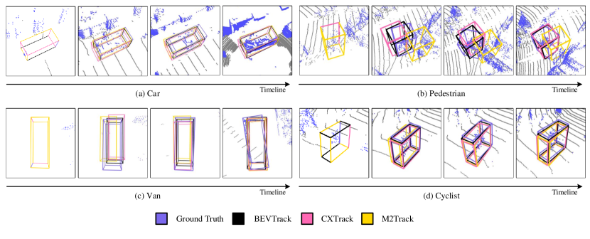
Figure 4: Visualization results on different KITTI categories: (a) Car; (b) Pedestrian; (c) Van; (d) Cyclist.

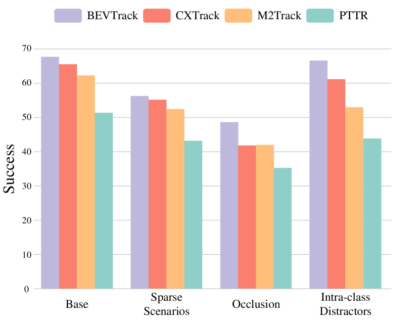
Figure 5: Robustness under different challenging scenes on KITTI Pedestrian category.

For a more comprehensive evaluation of effectiveness in challenging scenarios, we present results from various methods in cases characterized by sparse scenarios, occlusion, and intra-class distractors. To verify the effectiveness in sparse scenarios, we follow V2B [35] to select sparse scenes for evaluation according to the number of points lying in the target bounding boxes in the test set. For analysis of the impact of intra-class distractors, we pick out scenes that contain Pedestrian distractors close to the target from the KITTI test split. For the occlusion situations, we filter out scenes of occlusion scores less than one in the KITTI test set.

As shown in Fig. 5, each column from left to right represents the cases of base setting, sparse scenarios, occlusion, and intra-class distractors respectively on the Pedestrian category of the KITTI dataset. Our BEVTrack exhibits superior performance across all challenging scenarios, particularly excelling in cases involving occlusion and intra-class distractors. The Siamese paradigm represented by PTTR is susceptible due to hardly distinguishing targets by appearance in point clouds, suffering from a significant performance drop. While CXTrack effectively utilizes contextual information and is designed with a refined architecture, it still relies on appearance matching resulting in degraded performance. M2-Track eschews appearance matching, explicitly modeling the motion of the target but lacking sufficient utilization of contextual and spatial information, leading to suboptimal performance. Conversely, our proposed BEVTrack models the motion of both targets and intra-class distractors using BEV features, thereby harnessing contextual and spatial information effectively. This approach results in improved target localization accuracy, particularly in challenging scenarios.

TABLE II: Comparisons with the state-of-the-art methods on NuScenes dataset. Success/Precision are used for evaluation. Bold and underline denote the best and the second-best scores, respectively.

Method	Car (64159)	Pedestrian (33227)	Truck (13587)	Trailer (3352)	Bus (2953)	Mean by Class	Mean (117278)
SC3D	22.31 / 21.93	11.29 / 12.65	35.28 / 28.12	35.28 / 28.12	29.35 / 24.08	25.78 / 22.90	20.70 / 20.20
P2B	38.81 / 43.18	28.39 / 52.24	48.96 / 40.05	48.96 / 40.05	32.95 / 27.41	38.41 / 40.90	36.48 / 45.08
PTT	41.22 / 45.26	19.33 / 32.03	50.23 / 48.56	51.70 / 46.50	39.40 / 36.70	40.38 / 41.81	36.33 / 41.72
BAT	40.73 / 43.29	28.83 / 53.32	52.59 / 44.89	52.59 / 44.89	35.44 / 28.01	40.59 / 42.42	38.10 / 45.71
GLT-T	48.52 / 54.29	31.74 / 56.49	52.74 / 51.43	57.60 / 52.01	44.55 / 40.69	47.03 / 50.98	44.42 / 54.33
PTTR	51.89 / 58.61	29.90 / 45.09	45.30 / 44.74	45.87 / 38.36	43.14 / 37.74	43.22 / 44.91	44.50 / 52.07
M2Track	55.85 / 65.09	32.10 / 60.92	57.36 / 59.54	57.61 / 58.26	51.39 / 51.44	50.86 / 59.05	49.23 / 62.73
BEVTrack	63.91 / 70.72	45.60 / 74.93	61.73 / 60.84	65.39 / 59.91	57.95 / 53.59	58.92 / 64.00	58.36 / 70.03
Improvement	↑8.06 / ↑5.63	↑13.50 / ↑14.01	↑4.37 / ↑1.3	↑7.78 / ↑1.65	↑6.56 / ↑2.15	↑8.06 / ↑4.95	↑9.13 / ↑7.30

TABLE III: Comparisons with the state-of-the-art methods on Waymo Open Dataset. Success/Precision are used for evaluation. Bold and underline denote the best and the second-best scores, respectively.

Method	Vehicle(185731)				Pedestrian(241752)				Mean (427483)
	Easy	Medium	Hard	Mean	Easy	Medium	Hard	Mean
P2B	57.1 / 65.4	52.0 / 60.7	47.9 / 58.5	52.6 / 61.7	18.1 / 30.8	17.8 / 30.0	17.7 / 29.3	17.9 / 30.1	33.0 / 43.8
BAT	61.0 / 68.3	53.3 / 60.9	48.9 / 57.8	54.7 / 62.7	19.3 / 32.6	17.8 / 29.8	17.2 / 28.3	18.2 / 30.3	34.1 / 44.4
V2B	64.5 / 71.5	55.1 / 63.2	52.0 / 62.0	57.6 / 65.9	27.9 / 43.9	22.5 / 36.2	20.1 / 33.1	23.7 / 37.9	38.4 / 50.1
STNet	65.9 / 72.7	57.5 / 66.0	54.6 / 64.7	59.7 / 68.0	29.2 / 45.3	24.7 / 38.2	22.2 / 35.8	25.5 / 39.9	40.4 / 52.1
TAT	66.0 / 72.6	56.6 / 64.2	56.6 / 64.2	58.9 / 66.7	32.1 / 49.5	25.6 / 40.3	21.8 / 35.9	26.7 / 42.2	40.7 / 52.8
CXTrack	63.9 / 71.1	54.2 / 62.7	52.1 / 63.7	57.1 / 66.1	35.4 / 55.3	29.7 / 47.9	26.3 / 44.4	30.7 / 49.4	42.2 / 56.7
BEVTrack	66.1 / 71.7	56.8 / 64.7	55.6 / 66.1	59.8 / 67.7	42.1 / 65.0	34.6 / 56.2	29.9 / 50.4	35.8 / 57.5	46.2 / 61.9
Improvement	↑2.2 / ↑0.6	↑2.6 / ↑2.0	↑3.5 / ↑2.4	↑2.7 / ↑1.6	↑6.7 / ↑9.7	↑4.9 / ↑8.3	↑3.6 / ↑6.0	↑5.1 / ↑8.1	↑4.0 / ↑5.2

We also present the visual analysis of the tracking results under different challenging scenes on KITTI. As shown in Fig. 6, BEVTrack achieves good accuracy in different cases. When there are distractors around the target, conventional approaches tend to drift towards these distractors as a consequence of excessive dependence on appearance matching or segmentation. In contrast, our approach maintains accurate tracking by modeling the motion relations of not only the target itself but also distractors. In these challenging scenarios, our method can track point cloud objects more accurately and robustly.

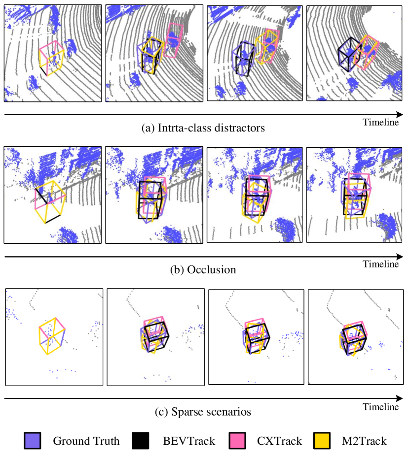
Figure 6: Visualization results under different challenging scenes on KITTI Pedestrian category: (a) Intra-class distractors; (b) Occlusion; (c) Sparse scenarios.

Results on Nuscenes.

NuScenes poses a more formidable challenge for the 3D SOT task compared to KITTI, primarily attributable to its larger data volumes and sparser annotations (2Hz for NuScenes versus 10Hz for KITTI and Waymo Open Dataset). Subsequently, following the methodology established by M2-Track, we perform a comparative evaluation on the NuScenes dataset against prior methodologies, namely SC3D [31], P2B [4], PTT [32], BAT [6], GLT-T [33], PTTR [8], and M2Track [5]. As shown in Table II, our method significantly outperforms the previous state-of-the-art technique, i.e., M2-Track. By efficiently leveraging the contextual and spatial information, BEVTrack exhibits superior performance over methods reliant on appearance matching or segmentation, especially in datasets like NuScenes with sparser point clouds.

Results on WOD.

To demonstrate the generalization ability of our proposed BEVTrack, we evaluate the KITTI pre-trained models on WOD and compare it with the previous state-of-the-art methods, including P2B [4], BAT [6], V2B [35], STNet [15], TAT [47], and CXTrack [11], following the previous work [45]. The experimental results, as presented in Table III, show that BEVTrack yields better tracking results than other methods under different levels of sparsity. In summary, our proposed approach excels in accurately tracking targets within challenging scenes and exhibits strong generalization capabilities across unseen scenarios.

Inference Speed.

Computational efficiency has always been an important fact of object tracking within practical real-world applications. The simple convolutional architecture employed by BEVTrack ensures real-time inference at an impressive speed of 201 FPS on a single NVIDIA GTX 4090 GPU, which is 4.48 times faster than the previously leading method, CX-Track [11]. The simplicity of BEVTrack’s pipeline facilitates flexible adjustments in model size by incorporating advanced backbones or devising more effective BMM modules to further enhance performance. This paper aims to establish a baseline model for 3D SOT and favors a lightweight structure to strike a balance between performance and efficiency. The exploration of more effective architectural designs remains a potential avenue for future research.

TABLE IV: Ablation study of BEV Feature Extraction Method.

Methods	Latency	Car	Pedestrian	Van	Cyclist	Mean
Pre-BEV	4.98 ms	71.7/84.1	68.4/92.7	65.7/76.2	75.5/94.6	69.8/87.4
Post-BEV	1.66 ms	67.4/80.9	64.1/90.3	63.6/76.1	73.4/94.3	65.8/84.8

TABLE V: Ablation study of the BMM module.

ratio	Car	Pedestrian	Van	Cyclist	Mean
1×	68.4/80.9	63.7/90.8	63.7/76.6	73.4/94.0	66.1/85.1
2×	70.7/82.1	62.7/90.0	65.3/75.2	72.4/93.9	66.8/85.2
4×	71.7/84.1	68.4/92.7	65.7/76.2	75.5/94.6	69.8/87.4
8×	71.4/83.8	65.0/91.5	66.1/76.4	72.7/93.7	68.2/86.7

TABLE VI: Ablation study of the regression strategy. ”G” refers to regress with Gaussian assumption, ”L” refers to regress with Laplace assumption and ”D” refers to regress with distribution-aware tracking strategy.

	Car	Pedestrian	Van	Cyclist	Mean
G	68.3/80.9	56.6/85.3	60.3/70.6	68.8/92.4	62.6/82.1
L	69.4/82.4	59.1/86.3	58.2/71.6	69.7/93.1	63.9/83.4
D	71.7/84.1	68.4/92.7	65.7/76.2	75.5/94.6	69.8/87.4

TABLE VII: Ablation study of the fusion method in BMM.

operation	Car	Pedestrian	Van	Cyclist	Mean
cat(c)	71.7/84.1	68.4/92.7	65.7/76.2	75.5/94.6	69.8/87.4
sum(+)	68.8/79.7	56.8/86.5	58.8/71.5	72.2/93.5	62.8/82.2
mul(×)	60.4/70.3	52.5/81.3	60.7/74.7	72.7/93.7	57.3/76.0
sub(-)	68.4/79.8	56.1/86.1	58.8/71.3	72.3/93.2	62.3/82.1

IV-C Ablation Studies

To validate the effectiveness of the design choice in bevTrack, we conduct ablation studies on the KITTI dataset.

BEV Features Extraction.

There are mainly two branches to convert point cloud data into BEV representation, i.e., Pre-BEV which extracts point cloud features in 3D space before converting point cloud data into BEV representation, and Post-BEV which extracts BEV features in BEV space directly. We make ablations on the backbone of 3D sparse CNN and 2D dense CNN, corresponding to the Pre-BEV and Post-BEV respectively, in Table IV. Pre-BEV paradigm employing 3D sparse CNN in the backbone yields accurate results but incurs high latency. This configuration serves as the default setting for BEVTrack. In contrast, when utilizing a 2D dense CNN as the backbone network with an equivalent number of layers and channels compared to the 3D counterpart, it achieves superior efficiency. Despite the performance degradation, it consistently outperforms the previous competitive method, e.g., M2Track, across all categories. It could be an alternative choice for our BEVTrack when favoring high computational efficiency.

Design Choice of the BMM Module.

As detailed in Sec. III-C, for tracking targets with diverse motion patterns, the motion modeling module necessitates sufficient receptive fields. Our approach enlarges receptive fields through spatial down-sampling of features, but sacrificing fine-grained detail information due to the resulting smaller feature maps. In order to reach a balance between sufficient receptive fields and fine-grained detail information, we compare the tracking accuracy when motion modeling is performed under different down-sampling ratios. For a fair comparison, the number of convolutional layers is the same in different settings. The results in Table V demonstrate that the 4$\times$ down-sampling configuration yields the best performance. Consequently, we adopt this configuration as the default setting.

Distribution-aware Regression.

To examine how the assumption of the output distribution affects the tracking performance, we compare the tracking results of utilizing different density functions as well as the proposed distribution-aware regression strategy. The Laplace distribution and Gaussian distribution will degenerate to standard $l_{1}$ and $l_{2}$ loss if they are assumed to have constant variances. As shown in Table VI, the distribution-aware regression approach achieves better performance than the regression with $l_{1}$ or $l_{2}$ loss, especially on the Success metric, which demonstrates the importance of learning the actual distribution. We visualize the distributions learned by normalizing flow across different categories in Fig. 7. The learned distribution has a sharper peak than the Gaussian distribution and a smoother edge than the Laplace distribution, while this difference demonstrates the importance of the distribution-aware optimization scheme. Furthermore, there are also differences between the learned distributions across different categories, implying that assuming all categories conform to a fixed Laplace or Gaussian distribution may be not optimal.

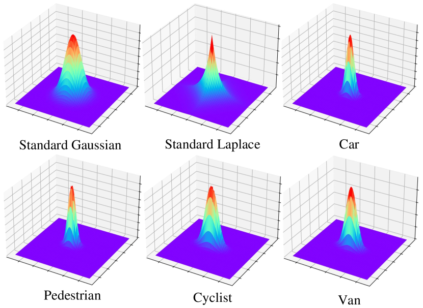
Figure 7: Visualization of the learned distributions.

Fusion Method in BMM.

Feature fusion propagates the target cues into the search area, which is a critical aspect of the 3D SOT task. We investigate various fusion techniques: concatenation (denoted as ’cat (c)’), summation (’sum (+)’), multiplication (’mul ($\times$)’), and subtraction (’sub (-)’). As shown in Table VII, the concatenation operation yields the best performance across all categories, outperforming others with a maximum improvement in precision and success of 12.5% and 11.4%, respectively. Consequently, we select concatenation as the default setting. It shows that an appropriate fusion method is important for tracking, and we believe that our method could benefit from more research progress in this direction.

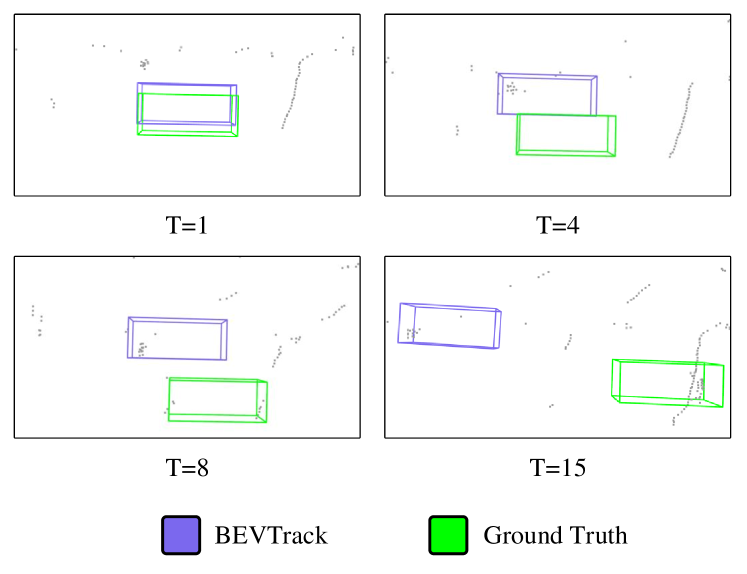
Figure 8: Tracking failure cases of our BEVTrack on extremely sparse point cloud scene.

V Discussion

While BEVTrack is robust to the most challenging scenarios, it tends to drift to background points when point clouds are extremely sparse to capture informative shapes or in situations of target disappearance due to occlusion. As shown in Fig. 8, though the target reappears in subsequent frames, the model has mistaken background points as the target, resulting in failures. Possible solutions are to incorporate temporal information and multi-modal information. In our experiments, we currently propagate target cues solely from the most recent frame to the current frame, thereby disregarding valuable information present in previous frames. Consequently, the model’s performance is suboptimal in scenarios of target disappearance due to occlusion. Fortunately, temporal information [48, 49, 50] can be readily introduced in BEVTrack, by concatenating additional temporal BEV features from preceding frames. Moreover, point clouds are typically incomplete and lack detailed textural structure, while image data captures comprehensive scene details, providing richer semantic and textural information for effective target discrimination. BEV, as the unified representation for multi-modal fusion [51, 52, 53], adeptly preserves semantic information from cameras and geometric information from LIDAR. We envision that BEVTrack can serve as an inspiration for further research into multi-frame, multi-modal fusion methodologies for SOT.

VI Conclution

This paper introduces BEVTrack, a simple yet strong baseline for 3D single object tracking (SOT). BEVTrack performs tracking within the Bird’s-Eye View representation, thereby effectively exploiting spatial information and capturing motion cues. Additionally, we propose a distribution-aware regression strategy that learns the actual distribution adapted to targets possessing diverse attributes, providing accurate guidance for tracking. Comprehensive experiments conducted on widely recognized benchmarks underscore BEVTrack’s efficacy, establishing its superiority over state-of-the-art tracking methods. Furthermore, it achieves a high inference speed of about 200 FPS. We hope this study could provide valuable insights to the tracking community and inspire further research on BEV-based 3D SOT methods.

References

- [1] T. Yin, X. Zhou, and P. Krahenbuhl, “Center-based 3d object detection and tracking,” in Proceedings of the IEEE Conference on Computer Vision and Pattern Recognition, 2021, pp. 11 784–11 793.
- [2] Y. Cai, L. Dai, H. Wang, and Z. Li, “Multi-target pan-class intrinsic relevance driven model for improving semantic segmentation in autonomous driving,” IEEE Transactions on Image Processing, vol. 30, pp. 9069–9084, 2021.
- [3] H.-k. Chiu, A. Prioletti, J. Li, and J. Bohg, “Probabilistic 3d multi-object tracking for autonomous driving,” arXiv preprint arXiv:2001.05673, 2020.
- [4] H. Qi, C. Feng, Z. Cao, F. Zhao, and Y. Xiao, “P2b: point-to-box network for 3d object tracking in point clouds,” in Proceedings of the IEEE Conference on Computer Vision and Pattern Recognition, 2020, pp. 6329–6338.
- [5] C. Zheng, X. Yan, H. Zhang, B. Wang, S. Cheng, S. Cui, and Z. Li, “Beyond 3d siamese tracking: A motion-centric paradigm for 3d single object tracking in point clouds,” in Proceedings of the IEEE/CVF International Conference on Computer Vision, 2022, pp. 8111–8120.
- [6] C. Zheng, X. Yan, J. Gao, W. Zhao, W. Zhang, Z. Li, and S. Cui, “Box-aware feature enhancement for single object tracking on point clouds,” in Proceedings of the IEEE/CVF International Conference on Computer Vision, 2021, pp. 13 199–13 208.
- [7] J. Nie, Z. He, Y. Yang, Z. Bao, M. Gao, and J. Zhang, “Osp2b: One-stage point-to-box network for 3d siamese tracking,” in Proceedings of the International Joint Conference on Artificial Intelligence, 2023.
- [8] C. Zhou, Z. Luo, Y. Luo, T. Liu, L. Pan, Z. Cai, H. Zhao, and S. Lu, “Pttr: Relational 3d point cloud object tracking with transformer,” in Proceedings of the IEEE Conference on Computer Vision and Pattern Recognition, 2022, pp. 8531–8540.
- [9] C. R. Qi, L. Yi, H. Su, and L. J. Guibas, “Pointnet++: Deep hierarchical feature learning on point sets in a metric space,” Advances in Neural Information Processing Systems, vol. 30, 2017.
- [10] Y. Wang, Y. Sun, Z. Liu, S. E. Sarma, M. M. Bronstein, and J. M. Solomon, “Dynamic graph cnn for learning on point clouds,” ACM Transactions on Graphics, p. 1–12, 2019.
- [11] T.-X. Xu, Y.-C. Guo, Y.-K. Lai, and S.-H. Zhang, “Cxtrack: Improving 3d point cloud tracking with contextual information,” in Proceedings of the IEEE Conference on Computer Vision and Pattern Recognition, 2023, pp. 1084–1093.
- [12] C. R. Qi, O. Litany, K. He, and L. J. Guibas, “Deep hough voting for 3d object detection in point clouds,” in Proceedings of the IEEE/CVF International Conference on Computer Vision, 2019, pp. 9277–9286.
- [13] Z. Fang, S. Zhou, Y. Cui, and S. Scherer, “3d-siamrpn: An end-to-end learning method for real-time 3d single object tracking using raw point cloud,” IEEE Sensors Journal, p. 4995–5011, 2021.
- [14] C. R. Qi, H. Su, K. Mo, and L. J. Guibas, “Pointnet: Deep learning on point sets for 3d classification and segmentation,” in Proceedings of the IEEE Conference on Computer Vision and Pattern Recognition, 2017, pp. 652–660.
- [15] L. Hui, L. Wang, L. Tang, K. Lan, J. Xie, and J. Yang, “3d siamese transformer network for single object tracking on point clouds,” in Proceedings of the European Conference on Computer Vision, 2022, pp. 293–310.
- [16] J. Nie, Z. He, Y. Yang, X. Lv, M. Gao, and J. Zhang, “Glt-t++: Global-local transformer for 3d siamese tracking with ranking loss,” arXiv preprint arXiv:2304.00242, 2023.
- [17] Z. Yang, Y. Wei, and Y. Yang, “Collaborative video object segmentation by foreground-background integration,” in Proceedings of the European Conference on Computer Vision, 2020, pp. 332–348.
- [18] P. Voigtlaender, Y. Chai, F. Schroff, H. Adam, B. Leibe, and L.-C. Chen, “Feelvos: Fast end-to-end embedding learning for video object segmentation,” in Proceedings of the IEEE Conference on Computer Vision and Pattern Recognition, 2019, pp. 9481–9490.
- [19] Y. Zhou and O. Tuzel, “Voxelnet: End-to-end learning for point cloud based 3d object detection,” in Proceedings of the IEEE Conference on Computer Vision and Pattern Recognition, 2018, pp. 4490–4499.
- [20] A. H. Lang, S. Vora, H. Caesar, L. Zhou, J. Yang, and O. Beijbom, “Pointpillars: Fast encoders for object detection from point clouds,” in Proceedings of the IEEE Conference on Computer Vision and Pattern Recognition, 2019, pp. 12 697–12 705.
- [21] J. Philion and S. Fidler, “Lift, splat, shoot: Encoding images from arbitrary camera rigs by implicitly unprojecting to 3d,” in Proceedings of the European Conference on Computer Vision, 2020, pp. 194–210.
- [22] A. Geiger, P. Lenz, and R. Urtasun, “Are we ready for autonomous driving? the kitti vision benchmark suite,” in Proceedings of the IEEE Conference on Computer Vision and Pattern Recognition, 2012, pp. 3354–3361.
- [23] H. Caesar, V. Bankiti, A. H. Lang, S. Vora, V. E. Liong, Q. Xu, A. Krishnan, Y. Pan, G. Baldan, and O. Beijbom, “Nuscenes: A multimodal dataset for autonomous driving,” in Proceedings of the IEEE Conference on Computer Vision and Pattern Recognition, 2020, pp. 11 621–11 631.
- [24] P. Sun, H. Kretzschmar, X. Dotiwalla, A. Chouard, V. Patnaik, P. Tsui, J. Guo, Y. Zhou, Y. Chai, B. Caine, V. Vasudevan, W. Han, J. Ngiam, H. Zhao, A. Timofeev, S. Ettinger, M. Krivokon, A. Gao, A. Joshi, Y. Zhang, J. Shlens, Z. Chen, and D. Anguelov, “Scalability in perception for autonomous driving: waymo open dataset,” in Proceedings of the IEEE Conference on Computer Vision and Pattern Recognition, 2020, pp. 2446–2454.
- [25] A. Pieropan, N. Bergström, M. Ishikawa, and H. Kjellström, “Robust 3d tracking of unknown objects,” in Proceedings of the IEEE International Conference on Robotics and Automation, 2015, pp. 2410–2417.
- [26] L. Spinello, K. Arras, R. Triebel, and R. Siegwart, “A layered approach to people detection in 3d range data,” in Proceedings of the AAAI Conference on Artificial Intelligence, 2010, pp. 1625–1630.
- [27] M. H. Abdelpakey and M. S. Shehata, “Dp-siam: Dynamic policy siamese network for robust object tracking,” IEEE Transactions on Image Processing, vol. 29, pp. 1479–1492, 2019.
- [28] S. Chan, J. Tao, X. Zhou, C. Bai, and X. Zhang, “Siamese implicit region proposal network with compound attention for visual tracking,” IEEE Transactions on Image Processing, vol. 31, pp. 1882–1894, 2022.
- [29] T. Xu, Z. Feng, X.-J. Wu, and J. Kittler, “Toward robust visual object tracking with independent target-agnostic detection and effective siamese cross-task interaction,” IEEE Transactions on Image Processing, vol. 32, pp. 1541–1554, 2023.
- [30] Z. Liu, X. Wang, Y. Zhong, M. Shu, and C. Sun, “Siamhyper: Learning a hyperspectral object tracker from an rgb-based tracker,” IEEE Transactions on Image Processing, vol. 31, pp. 7116–7129, 2022.
- [31] S. Giancola, J. Zarzar, and B. Ghanem, “Leveraging shape completion for 3d siamese tracking,” in Proceedings of the IEEE Conference on Computer Vision and Pattern Recognition, 2019, pp. 1359–1368.
- [32] J. Shan, S. Zhou, Z. Fang, and Y. Cui, “Ptt: Point-track-transformer module for 3d single object tracking in point clouds,” in Proceedings of the IEEE/RSJ International Conference on Intelligent Robots and Systems, 2021, pp. 1310–1316.
- [33] J. Nie, Z. He, Y. Yang, M. Gao, and J. Zhang, “Glt-t: Global-local transformer voting for 3d single object tracking in point clouds,” in Proceedings of the AAAI Conference on Artificial Intelligence, 2023, pp. 1957–1965.
- [34] A. Vaswani, N. Shazeer, N. Parmar, J. Uszkoreit, L. Jones, A. Gomez, L. Kaiser, and I. Polosukhin, “Attention is all you need,” Advances in neural information processing systems, vol. 30, 2017.
- [35] L. Hui, L. Wang, M. Cheng, J. Xie, and J. Yang, “3d siamese voxel-to-bev tracker for sparse point clouds,” Advances in Neural Information Processing Systems, vol. 34, pp. 28 714–28 727, 2021.
- [36] H. Li, C. Sima, J. Dai, W. Wang, L. Lu, H. Wang, E. Xie, Z. Li, H. Deng, H. Tian et al., “Delving into the devils of bird’s-eye-view perception: A review, evaluation and recipe,” arXiv preprint arXiv:2209.05324, 2022.
- [37] T. Yin, X. Zhou, and P. Krahenbuhl, “Center-based 3d object detection and tracking,” in Proceedings of the IEEE Conference on Computer Vision and Pattern Recognition, 2021, pp. 11 784–11 793.
- [38] Y. Wang and J. M. Solomon, “Object dgcnn: 3d object detection using dynamic graphs,” Advances in Neural Information Processing Systems, vol. 34, pp. 20 745–20 758, 2021.
- [39] X. Chen, H. Ma, J. Wan, B. Li, and T. Xia, “Multi-view 3d object detection network for autonomous driving,” in Proceedings of the IEEE Conference on Computer Vision and Pattern Recognition, 2017, pp. 1907–1915.
- [40] B. Graham and L. Van der Maaten, “Submanifold sparse convolutional networks,” arXiv preprint arXiv:1706.01307, 2017.
- [41] B. Graham, M. Engelcke, and L. Van Der Maaten, “3d semantic segmentation with submanifold sparse convolutional networks,” in Proceedings of the IEEE Conference on Computer Vision and Pattern Recognition, 2018, pp. 9224–9232.
- [42] J. Li, S. Bian, A. Zeng, C. Wang, B. Pang, W. Liu, and C. Lu, “Human pose regression with residual log-likelihood estimation,” in Proceedings of the IEEE/CVF International Conference on Computer Vision, 2021, pp. 11 025–11 034.
- [43] L. Dinh, J. Sohl-Dickstein, and S. Bengio, “Density estimation using real nvp,” in Proceedings of the International Conference on Learning Representations, 2016.
- [44] A. L. Maas, A. Y. Hannun, A. Y. Ng et al., “Rectifier nonlinearities improve neural network acoustic models,” in Proceedings of the International Conference on Machine Learning, vol. 30, 2013.
- [45] Z. Pang, Z. Li, and N. Wang, “Model-free vehicle tracking and state estimation in point cloud sequences,” in Proceedings of the IEEE/RSJ International Conference on Intelligent Robots and Systems, 2021, pp. 8075–8082.
- [46] M. Kristan, J. Matas, A. Leonardis, T. Vojir, R. Pflugfelder, G. Fernandez, G. Nebehay, F. Porikli, and L. Cehovin, “A novel performance evaluation methodology for single-target trackers,” IEEE Transactions on Pattern Analysis and Machine Intelligence, p. 2137–2155, 2016.
- [47] K. Lan, H. Jiang, and J. Xie, “Temporal-aware siamese tracker: Integrate temporal context for 3d object tracking,” in Proceedings of the IEEE Conference on Computer Vision and Pattern Recognition, 2022, pp. 399–414.
- [48] J. Huang and G. Huang, “Bevdet4d: Exploit temporal cues in multi-camera 3d object detection,” arXiv preprint arXiv:2203.17054, 2022.
- [49] B. Huang, Y. Li, E. Xie, F. Liang, L. Wang, M. Shen, F. Liu, T. Wang, P. Luo, and J. Shao, “Fast-bev: Towards real-time on-vehicle bird’s-eye view perception,” arXiv preprint arXiv:2301.07870, 2023.
- [50] Z. Li, W. Wang, H. Li, E. Xie, C. Sima, T. Lu, Y. Qiao, and J. Dai, “Bevformer: Learning bird’s-eye-view representation from multi-camera images via spatiotemporal transformers,” in Proceedings of the European Conference on Computer Vision, 2022, pp. 1–18.
- [51] Z. Liu, H. Tang, A. Amini, X. Yang, H. Mao, D. L. Rus, and S. Han, “Bevfusion: Multi-task multi-sensor fusion with unified bird’s-eye view representation,” in Proceedings of the IEEE International Conference on Robotics and Automation, 2023, pp. 2774–2781.
- [52] X. Bai, Z. Hu, X. Zhu, Q. Huang, Y. Chen, H. Fu, and C.-L. Tai, “Transfusion: Robust lidar-camera fusion for 3d object detection with transformers,” in Proceedings of the IEEE Conference on Computer Vision and Pattern Recognition, 2022, pp. 1090–1099.
- [53] T. Liang, H. Xie, K. Yu, Z. Xia, Z. Lin, Y. Wang, T. Tang, B. Wang, and Z. Tang, “Bevfusion: A simple and robust lidar-camera fusion framework,” Advances in Neural Information Processing Systems, vol. 35, pp. 10 421–10 434, 2022.