Integral equation methods for acoustic scattering by fractals

Abstract

We study sound-soft time-harmonic acoustic scattering by general scatterers, including fractal scatterers, in 2D and 3D space. For an arbitrary compact scatterer $\Gamma$ we reformulate the Dirichlet boundary value problem for the Helmholtz equation as a first kind integral equation (IE) on $\Gamma$ involving the Newton potential. The IE is well-posed, except possibly at a countable set of frequencies, and reduces to existing single-layer boundary IEs when $\Gamma$ is the boundary of a bounded Lipschitz open set, a screen, or a multi-screen. When $\Gamma$ is uniformly of $d$-dimensional Hausdorff dimension in a sense we make precise (a $d$-set), the operator in our equation is an integral operator on $\Gamma$ with respect to $d$-dimensional Hausdorff measure, with kernel the Helmholtz fundamental solution, and we propose a piecewise-constant Galerkin discretization of the IE, which converges in the limit of vanishing mesh width. When $\Gamma$ is the fractal attractor of an iterated function system of contracting similarities we prove convergence rates under assumptions on $\Gamma$ and the IE solution, and describe a fully discrete implementation using recently proposed quadrature rules for singular integrals on fractals. We present numerical results for a range of examples and make our software available as a Julia code.

1 Introduction

This paper, prepared in large part during a recent Isaac Newton Institute programme on multiple wave scattering, is concerned with one of the central themes of that programme, the classical problem of scattering of time-harmonic acoustic waves in $\mathbb{R}^{n}$, $n=2$ or $3$, by a scatterer $\Gamma$ that may have multiple components or other complicated geometrical features. This paper treats the sound-soft case, where the total field $u^{t}$ vanishes on $\Gamma$, which we assume throughout is a compact subset of $\mathbb{R}^{n}$. Our particular interest is in scattering by fractals, which provide a model for the multiscale roughness of many natural and man-made scatterers.

The classical formulation of this scattering problem as a boundary value problem (BVP) requires that the scattered field $u$ satisfies the Helmholtz equation (18) in the open set $\Omega:=\mathbb{R}^{n}\setminus\Gamma$ and the standard Sommerfeld radiation condition (19), and enforces the sound-soft boundary condition by the requirement that $u^{t}\in W_{0}^{1,{\rm loc}}(\Omega)$, the “local” version of the space $W^{1}_{0}(\Omega)$, which is the closure of $C_{0}^{\infty}(\Omega)$ in the classical Sobolev space $W^{1}(\Omega):=\{v\in L^{2}(\Omega):\nabla v\in L^{2}(\Omega)\}$ (the function space notations we use are recalled in §2.2 below). It is well-known that, as long as BVP uniqueness holds, which is the case, in particular, if $\Omega$ is connected, then this BVP is well-posed for every compact $\Gamma$. Moreover, the associated variational formulation, obtained by Green’s theorem and use of an exact Dirichlet-to-Neumann map on the outer boundary of a bounded truncation of $\Omega$, has a sesquilinear form that is a compact perturbation of a coercive form (e.g., [11, §3]), so that standard Galerkin finite element methods are convergent.

This paper concerns integral equation (IE) formulations of this scattering problem and their numerical solution. The contributions of the paper are several. Firstly, we write down in §3 a novel IE formulation of this problem that applies for every compact $\Gamma\subset\mathbb{R}^{n}$. For this, the scattered field is sought as an acoustic Newton potential $u=\mathcal{A}\phi$, with an unknown density $\phi\in H^{-1}_{\Gamma}$, where $H^{-1}_{\Gamma}$ denotes the set of distributions in the classical Sobolev space $H^{-1}(\mathbb{R}^{n})$ that are supported in $\Gamma$. Provided BVP uniqueness holds, the boundary condition leads to a well-posed first-kind IE

$$A\phi=g,$$ (1)

such that $u=\mathcal{A}\phi$ is the unique solution to the scattering problem. The operator $A$, an isomorphism from $H_{\Gamma}^{-1}$ to its dual space, is a generalisation of the classical single-layer boundary integral operator, in cases where this is well-defined. Importantly, $A$ is a compact perturbation of a coercive operator, so that all Galerkin solution methods are convergent. These results provide an IE-based proof of well-posedness of the BVP for general compact $\Gamma$, generalising existing IE-based proofs for cases where $\Omega$ is Lipschitz or smoother (e.g., [24, Thm 9.11]).

We focus mostly on the particular case where $\Gamma$ is a $d$-set (definition (3) below), which means (roughly speaking) that $\Gamma$ is uniformly of Hausdorff dimension $d$, for some integer or fractional $d\in(0,n]$. If $H^{-1}_{\Gamma}=\{0\}$, which holds in the case that $\Gamma$ is a $d$-set if and only if $d\leq n-2$ (as we recall in §3), then by Theorem 3.4 the unique solution to (1) is $\phi=0$ (with $g$ necessarily zero), so that $u=\mathcal{A}\phi=0$; the scatterer is invisible to incident waves. To focus on cases where $u\neq 0$ we restrict our study to the range $n-2<d\leq n$.

(a) Closure of a
bounded Lipschitz
open set

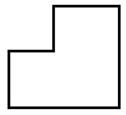
(b) Boundary of a
bounded Lipschitz
open set

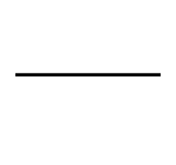
(c) Line segment
screen      

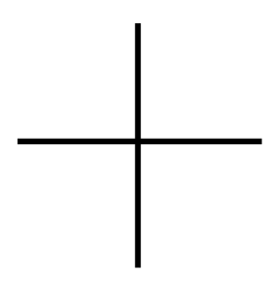
(d) Multi-screen

(e) Cantor set screen

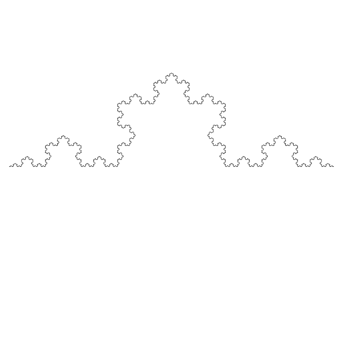
(f) Koch curve

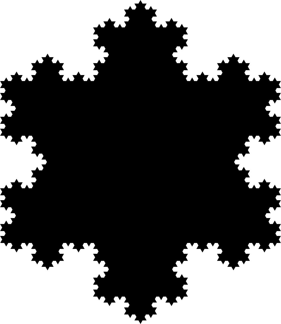
(g) Koch snowflake

Figure 1: Examples of $d$-sets in two-dimensional space ($n=2$), with: a) $d=2$; b) $d=1$; c) $d=1$; d) $d=1$; e) $d=\log(2)/\log(3)\approx 0.63$; f) $d=\log(4)/\log(3)\approx 1.26$; g) $d=2$. For details see text.

(a) $\rho=1/2$, non-disjoint

(b) $\rho=3/8$, disjoint

Figure 2: Sierpinski tetrahedron $d$-sets in 3D space, attractors of the IFS (6) for $\rho=1/2$ ($d=2$) and $\rho=3/8$ ($d=\log{4}/\log(8/3)\approx 1.41$).

A range of examples with $n-2<d\leq n$, relevant to our later discussions and computations, is pictured in Figures 1 and 2. Figure 1 shows examples in 2D space ($n=2$), namely: (a) $\Gamma=\overline{D}$ is the closure of a bounded Lipschitz open set $D$ ($d=n=2$); (b) $\Gamma=\partial D$ is the boundary of the same set ($d=n-1=1$); (c) $\Gamma=[0,1]\times\{0\}$ is a line segment ($d=n-1=1$); (d) $\Gamma=[-1,1]\times\{0\}\cup\{0\}\times[-1,1]$ is the cross formed by two line segments, an example of a multi-screen in the sense of [12] (all such multi-screens are $d$-sets with $d=n-1$); (e) $\Gamma=C\times\{0\}$, where $C\subset[0,1]$ is the classical middle-third Cantor set ($d=\log(2)/\log(3)\approx 0.6309$); (f) $\Gamma$ is the Koch curve ($d=\log(4)/\log(3)\approx 1.262$); (g) $\Gamma$ is the closure of the Koch snowflake domain ($d=2$).

Examples (c) and (e)-(g) in Figure 1 are all fixed points (attractors) of an iterated function system (IFS) satisfying the standard open set condition (OSC) (we recall these definitions in §2.1). As we recall in §2.1, every such IFS attractor is a $d$-set, with $d$ its fractal (Hausdorff) dimension. Figure 2 shows examples in 3D space ($n=3$) where $\Gamma$ is an IFS attractor that is a Sierpinski tetrahedron, with $d=2$ and $d=\log{4}/\log(8/3)\approx 1.41$. (We show numerical simulations for these examples in §5.) These examples make clear that our results are inclusive of multiple scattering cases where $\Gamma$ has complicated geometries and/or multiple components. Indeed, the IFS attractor examples Figure 1(e) and Figure 2(b) are both fractal cases where the IFS is disjoint (as defined in §2.1) so that $\Gamma$ is totally disconnected and has uncountably many components!

A key result, important both theoretically and computationally, is that in the $d$-set case we can interpret the Newton potential $\mathcal{A}\phi$ as an integral with respect to $\mathcal{H}^{d}$, $d$-dimensional Hausdorff measure (which coincides, under the appropriate normalisation [14, Defn. 2.1], with ordinary Lebesgue measure if $d=n$ [14, Thm. 2.5]). Precisely, if $\Psi\in\mathbb{L}_{2}(\Gamma)$, the space of complex-valued functions that are square integrable with respect to $\mathcal{H}^{d}|_{\Gamma}$, and $\mathrm{tr}_{\Gamma}^{*}\Psi$ denotes the associated distribution in $H_{\Gamma}^{-1}\subset H^{-1}(\mathbb{R}^{n})$, we have that

$$\mathcal{A}\mathrm{tr}_{\Gamma}^{*}\Psi(x)=\int_{\Gamma}\Phi(x,y)\Psi(y)\,\mathrm{d}\mathcal{H}^{d}(y),\quad x\in\Omega,$$ (2)

where $\Phi(x,y):={\mathrm{e}}^{{\mathrm{i}}k|x-y|}/(4\pi|x-y|)$ ($n=3$), $\Phi(x,y):=({\mathrm{i}}/4)H^{(1)}_{0}(k|x-y|)$ ($n=2$), is the standard fundamental solution of the Helmholtz equation, and $H_{0}^{(1)}$ is the Hankel function of the first kind of order zero (e.g., [1, Equation (9.1.3)]). Similarly, we show in §3.1 that the operator $A$ in (1) can be written equivalently as an integral operator $\mathbb{A}:=\mathrm{tr}_{\Gamma}\,A\,\mathrm{tr}_{\Gamma}^{*}$ with respect to $\mathcal{H}^{d}$ measure; here $\mathrm{tr}_{\Gamma}:H^{1}(\mathbb{R}^{n})\to\mathbb{L}_{2}(\Gamma)$ is the trace operator introduced in §2.2 ($\mathrm{tr}_{\Gamma}^{*}$ is its adjoint).

If $d=n$ (e.g., Figure 1(a), (g)), so that $\mathcal{H}^{d}$ is $n$-dimensional Lebesgue measure, (2) is a volume integral and (1) is equivalent to a volume IE on $\Gamma$. If $d=n-1$ and $\Gamma$ is the whole or part of the boundary of a bounded Lipschitz open set (e.g., Figure 1(b), (c)), or is a multi-screen in the sense of [12] (e.g., Figure 1(d)), then $\mathcal{H}^{d}$ is standard surface measure (e.g., [14, Theorem 3.8]), (2) is a surface integral, specifically an acoustic single-layer potential, and (1) is equivalent to a standard first kind boundary IE (see Remark 3.10). Finally, in the case when $\Gamma$ is a subset of a hyperplane (e.g., Figure 1(c), (e)), our formulation reduces to cases studied recently in [9, 7, 10, 5, 4]. In particular, our results and methods build on those in [5, 4] where we study scattering by fractal planar screens that are $d$-sets with $n-2<d\leq n-1$.

In the $d$-set case we are able to show that the integral operator $\mathbb{A}$ is a continuous mapping on a scale of Sobolev-type spaces on $\Gamma$ (Proposition 3.11), a first step in a regularity theory for solutions of (1). In this case we are also able to propose (in §4) a concrete Galerkin IE method (IEM) in which $\Gamma$ is divided into a mesh of $N$ elements of maximum diameter $h$, $\mathbb{V}_{N}\subset\mathbb{L}_{2}(\Gamma)$ denotes the space of functions that are constant on each element of the mesh, and we seek a Galerkin approximation $\phi_{N}\in V_{N}:=\mathrm{tr}_{\Gamma}^{*}(\mathbb{V}_{N})\subset H^{-1}_{\Gamma}$ to the solution $\phi\in H^{-1}_{\Gamma}$ of (1). As long as $h\to 0$ as $N\to\infty$, best approximation results that follow from the density of $\mathrm{tr}_{\Gamma}^{*}(\mathbb{L}_{2}(\Gamma))$ in $H^{-1}_{\Gamma}$, coupled with standard functional analysis arguments, show that $\phi_{N}$ is well-defined for all sufficiently large $N$ and that $\phi_{N}\to\phi$ in $H^{-1}(\mathbb{R}^{n})$ norm (Theorem 4.1). Moreover, the entries of the matrix and right-hand-side of the linear system (50), defining the Galerkin solution, are given explicitly as double and single integrals, respectively, with respect to $\mathcal{H}^{d}$ measure.

Our strongest results (see §4.1) are for the special $d$-set case where $\Gamma$ is the attractor of an IFS satisfying the OSC (e.g., Figure 1(c), (e)-(g), Figure 2). In this case we are able to show, in the case $d<n$ and when $\Gamma$ is disjoint (e.g., Figure 1(e), Figure 2(b)) and in the case that $d=n$ (e.g., Figure 1(g)), that our scale of Sobolev spaces on $\Gamma$ is an interpolation scale in the sense of [8, Rem. 3.8], and, employing operator interpolation results, to show the regularity result that, for some $\epsilon\in(0,t_{d^{\prime}})$, where $t_{d^{\prime}}:=1-(n-d^{\prime})/2$ and $d^{\prime}$ is the Hausdorff dimension of the boundary of the unbounded component of $\Omega$, it holds that $\phi\in H^{-1+s}_{\Gamma}$ for $s<\epsilon$. Adapting the arguments and best approximation results from [5], which in turn depend on wavelet characterisations of Sobolev space norms on $\Gamma$ due to Jonsson [20], and using additional best approximation results for the case $d=n$ from [5], we also show (see Theorem 4.2 and the comments preceding it) that, if $\Gamma$ is disjoint or $d=n$, and $\phi\in H_{\Gamma}^{-1+s}$, then $\|\phi-\phi_{N}\|_{H^{-1}(\mathbb{R}^{n})}\leq ch^{s}\|\phi\|_{H^{-1+s}(\mathbb{R}^{n})}$ for all sufficiently large $N$. We show, moreover, that approximations to linear functionals of the solution, e.g. the approximation $u_{N}(x):=\mathcal{A}\phi_{N}(x)$ to $u(x)$ at some $x\in\Omega$, converge at the rate $h^{2s}$. Assuming a plausible conjecture that our regularity result holds with $\epsilon=t_{d^{\prime}}$, these results imply convergence rates of $h^{s}$ and $h^{2s}$, respectively, for every $s<t_{d^{\prime}}$.

In this $d$-set case where $\Gamma$ is an IFS attractor satisfying the OSC, we also propose in §4.2 a fully discrete implementation, evaluating our Hausdorff single and double integrals using recently proposed quadrature methods for singular integrals on IFS attractors [17, 16].

In §5 we show computations using our fully discrete Galerkin IEM, solving (1) and computing the scattered field $u=\mathcal{A}\phi$ for scatterers $\Gamma$ including the examples in Figure 2. This section includes numerical experiments exploring the convergence of our methods. These suggest that the regularity conjecture $\epsilon=t_{d^{\prime}}$ is true for many of the examples we study (the cases with $d^{\prime}<n-1$), and that the conditions of Theorem 4.2, established only for the disjoint IFS case, for $d=n$, and for particular $d=n-1$ cases, may be satisfied generally whenever $\Gamma$ is an IFS attractor satisfying the OSC (establishing this, and proving some version of a regularity conjecture, are both open problems).

An alternative approach to the simulation of scattering by fractals is to approximate the fractal by a smoother “prefractal” scatterer and apply a more conventional numerical method to the resulting approximate scattering problem. This was the approach taken in [10, 2], and in the earlier work in [19] and [26] for Laplace and elasticity problems. An achievement of [10, 2] was to prove convergence (without rates) of conventional BEMs for prefractal approximations of fractal screen problems, via Mosco convergence techniques. In principle, a similar analysis could be carried out for the problems under consideration in the current paper. However, we do not pursue this here.

Let us briefly outline the rest of the paper. In §2 we recall notations, definitions, and results that we need through the rest of the paper. Our results at a continuous level concerning our BVP and IE formulations are contained in §3. In §4, as noted above, we propose and analyse the convergence of our Galerkin IEM. §5 contains our numerical results.

2 Preliminaries

Throughout, for $n\in\mathbb{N}$ and $E\subset\mathbb{R}^{n}$, $\overline{E}$, $\partial E$, and $E^{\circ}=\overline{E}\setminus\partial E$ denote the closure, boundary, and interior of $E$ with respect to the standard Euclidean metric on $\mathbb{R}^{n}$, and $E^{c}:=\mathbb{R}^{n}\setminus E$ its complement in $\mathbb{R}^{n}$. In the case that $E$ is measurable, $m(E)$ denotes its $n$-dimensional Lebesgue measure. $B_{r}(x)\subset\mathbb{R}^{n}$ denotes the closed ball of radius $r$ centred on $x$.

2.1 Hausdorff measure and dimension, $d$-sets, IFS attractors

For $0\leq d\leq n$ let $\mathcal{H}^{d}$ denote the Hausdorff $d$-measure on $\mathbb{R}^{n}$ and let ${\rm dim_{H}}(S)\in[0,n]$ denote the Hausdorff dimension of $S\subset\mathbb{R}^{n}$ (see, e.g., [15]). As in [21, §1.1] and [31, §3], given $0<d\leq n$, we say a closed set $\Gamma\subset\mathbb{R}^{n}$ is a $d$-set if there exist $c_{2}>c_{1}>0$ such that

$$c_{1}r^{d}\leq\mathcal{H}^{d}\big{(}\Gamma\cap B_{r}(x)\big{)}\leq c_{2}r^{d},\qquad x\in\Gamma,\quad 0<r\leq 1.$$ (3)

If $\Gamma$ is a $d$-set then ${\rm dim_{H}}(\Gamma)=d$.

By an iterated function system of contracting similarities (we abbreviate this whole phrase as IFS) we mean a collection $\{s_{1},s_{2},\ldots,s_{M}\}$, for some $M\geq 2$, where, for each $m=1,\ldots,M$, $s_{m}:\mathbb{R}^{n}\to\mathbb{R}^{n}$, with $|s_{m}(x)-s_{m}(y)|=\rho_{m}|x-y|$, $x,y\in\mathbb{R}^{n}$, for some $\rho_{m}\in(0,1)$. The attractor of the IFS is the unique non-empty compact set $\Gamma$ satisfying

$$\Gamma=s(\Gamma),\quad\mbox{where}\quad s(E):=\bigcup_{m=1}^{M}s_{m}(E),\quad E\subset\mathbb{R}^{n}.$$ (4)

We shall restrict our attention to IFSs that satisfy the standard open set condition (OSC) [15, (9.11)], which implies that the attractor $\Gamma$ is a $d$-set (see, e.g., [31, Thm. 4.7]), where $d\in(0,n]$ is the unique solution of $\sum_{m=1}^{M}(\rho_{m})^{d}=1$. For a homogeneous IFS, where $\rho_{m}=\rho\in(0,1)$ for $m=1,\ldots,M$, we have $d=\log(M)/\log(1/\rho)$. Returning to the general, not necessarily homogeneous case, the OSC also implies (again, see [31, Thm. 4.7]) that $\Gamma$ is self-similar, meaning that the sets

$$\Gamma_{m}:=s_{m}(\Gamma),\qquad m=1,\ldots,M,$$ (5)

satisfy $\mathcal{H}^{d}(\Gamma_{m}\cap\Gamma_{m^{\prime}})=0$, $m\neq m^{\prime}$, so that $\Gamma$ is decomposed by (4) into $M$ similar copies of itself whose pairwise intersections have Hausdorff measure zero. For many of our results we make the additional assumption that the sets $\Gamma_{1},\ldots,\Gamma_{M}$ are disjoint. If this holds we say that the IFS attractor $\Gamma$ is disjoint, the OSC is automatically satisfied (e.g., [5, Lem. 2.5]), and $d<n$ (e.g. [5, Lemma 2.6]).

The following construction makes clear that if $C$ is an IFS attractor in dimension $n-1$ then $C\times\{0\}$ is an IFS attractor in dimension $n$.

Remark 2.1 (Lifting attractors to higher dimensions).

Suppose that $M\geq 2$ and that $S=\{s_{1},s_{2},\ldots,s_{M}\}$ is an IFS on $\mathbb{R}^{n}$. For $m=1,\ldots,M$, define $\tilde{s}_{m}:\mathbb{R}^{n+1}\to\mathbb{R}^{n+1}$ by $\tilde{s}_{m}((x,t))=(s_{m}(x),\rho_{m}t)$, for $x\in\mathbb{R}^{n}$, $t\in\mathbb{R}$. Then, for $m=1,\ldots,M$, $\tilde{s}_{m}$ is a contracting similarity with the same contraction factor $\rho_{m}$ as $s_{m}$, so that $\widetilde{S}=\{\tilde{s}_{1},\tilde{s}_{2},\ldots,\tilde{s}_{M}\}$ is an IFS on $\mathbb{R}^{n+1}$. Further, $\widetilde{S}$ satisfies the OSC/is disjoint if the same holds for $S$. If $\Gamma$ is the attractor of $S$ then $\widetilde{\Gamma}:=\Gamma\times\{0\}=\{(x,0):x\in\Gamma\}$ is the attractor of $\widetilde{S}$, and if the OSC holds for $S$ then $\Gamma$ and $\widetilde{\Gamma}$ are both $d$-sets with the same value of $d$.

Example 2.2 (Cantor set examples of IFS attractors).

Let $S=\{s_{1},s_{2}\}$, where $s_{m}:\mathbb{R}\to\mathbb{R}$, $m=1,2$, are defined, for some $\rho\in(0,1/2]$, by

$$s_{1}(t)=\rho t,\qquad s_{2}(t)=1+\rho(t-1),\qquad t\in\mathbb{R}.$$

Then $S$ is a homogeneous IFS with attractor $C$ that is the “middle-$(1-2\rho)$” Cantor set, given by

$$C=\bigcap_{n=0}^{\infty}C_{n},\quad\mbox{where}\quad C_{0}:=[0,1],\;\;C_{n}:=s(C_{n-1}),\;\;n\in\mathbb{N},$$

and $s$ is the mapping given by (4) on the set of subsets of $\mathbb{R}$. In the case $\rho=1/2$, $C=C_{n}=[0,1]$ for each $n$. If $0<\rho<1/2$ then $C_{n}$ is a union of $2^{n}$ disjoint closed intervals and $C_{n}$ is obtained from $C_{n-1}$ by removing the middle $(1-2\rho)$ from each of the intervals comprising $C_{n-1}$. This IFS satisfies the OSC (see [15, §9.2]), so that (see above) it is a $d$-set with $d=\dim_{H}(C)=\log(2)/\log(1/\rho)$. The attractor $C$ is disjoint if $\rho<1/2$. By Remark 2.1, $C\times\{0\}\subset\mathbb{R}^{2}$, shown for $\rho=1/2$ and $\rho=1/3$ in Figure 1(c) and (e), respectively, is also the attractor of an IFS, is a $d$-set with the same value of $d$, and is disjoint if $\rho<1/2$.

Example 2.3 (Koch curve).

The Koch curve $\Gamma\subset\mathbb{R}^{2}$, shown in Figure 1(f), is the attractor of the homogeneous IFS $\{s_{1},s_{2},s_{3},s_{4}\}$, where the mappings $s_{m}:\mathbb{R}^{2}\to\mathbb{R}^{2}$, $m\in\{1,\ldots,4\}$, are given by

$$s_{1}(x)=x/3, s_{2}(x)=Rx/3+\left(\begin{array}[]{c}\frac{1}{3}\\ 0\end{array}\right),\;\;$$

$$s_{3}(x)=R^{-1}x/3+\left(\begin{array}[]{c}\frac{1}{2}\\ \frac{1}{2\sqrt{3}}\end{array}\right),\;\; s_{4}(x)=x/3+\left(\begin{array}[]{c}\frac{2}{3}\\ 0\end{array}\right),$$

for $x\in\mathbb{R}^{2}$, where $R$ is the (orthogonal) rotation matrix for rotation counter-clockwise by angle $\pi/3$. $S$ satisfies the OSC (e.g., [15, Ex. 9.5]) and so $\Gamma$ is a $d$-set with $d=\log(4)/\log(3)\approx 1.26$. By Remark 2.1, $\Gamma\times\{0\}\subset\mathbb{R}^{3}$ is also the attractor of a homogeneous IFS, and is a $d$-set with the same value of $d$.

Example 2.4 (Koch snowflake).

The Koch snowflake $\Gamma\subset\mathbb{R}^{2}$, shown in Figure 1(g), is the attractor of a non-homogeneous IFS of 7 contracting similarities satisfying the OSC. It is non-disjoint and has dimension $d=2$. For details see [16, §5.4].

Example 2.5 (Sierpinski tetrahedron).

A Sierpinski tetrahedron $\Gamma\subset\mathbb{R}^{3}$ can be defined, for every $0<\rho\leq 1/2$, as the attractor of an IFS of four contracting similarities:

$$s_{i}(x)=x_{i}+\rho(x-x_{i}),\qquad i=1,\ldots,4,$$ (6)

where the $x_{i}$ are the vertices of a unit tetrahedron, explicitly

$$x_{1}=(0,0,0)^{T},\; x_{2}=(1,0,0)^{T},\;$$

$$x_{3}=(1/2,\sqrt{3}/2,0)^{T},\; x_{4}=(1/2,1/(2\sqrt{2}),\sqrt{5}/(2\sqrt{2}))^{T}.$$

$\Gamma$ is shown in Figure 2 for $\rho=3/8$ and $\rho=1/2$. It satisfies the OSC, has dimension $d=\log 4/\log(1/\rho)$, and is disjoint for $0<\rho<1/2$ but not for $\rho=1/2$.

2.2 Function spaces

Our Sobolev space notation follows that of [24] and [5]. For $s\in\mathbb{R}$ let $H^{s}{(\mathbb{R}^{n})}$ denote the usual Bessel potential Sobolev space. For a non-empty open set $\Omega\subset\mathbb{R}^{n}$, where $C_{0}^{\infty}(\Omega)$ is the set of those $C^{\infty}$ functions that are compactly supported in $\Omega$, we define $\widetilde{H}{}^{s}(\Omega):=\overline{C_{0}^{\infty}(\Omega)}^{H^{s}(\mathbb{R}^{n})}$ and, for $s\geq 0$, let $\accentset{\smash{\raisebox{-0.3014pt}{$\scriptstyle\circ$}}}{H}\rule{0.0pt}{9.90276pt}{}^{s}(\Omega)$ denote the subspace of those $\psi\in H^{s}(\mathbb{R}^{n})$ that are zero almost everywhere in $\Omega^{c}$ with respect to $n$-dimensional Lebesgue measure. We denote by $H^{s}(\Omega)$ the space of restrictions to $\Omega$ of elements of $H^{s}(\mathbb{R}^{n})$, equipped with the quotient norm $\|u\|_{H^{s}(\Omega)}:=\inf_{\begin{subarray}{c}\varphi\in H^{s}{(\mathbb{R}^{n})}\\ \varphi|_{\Omega}=u\end{subarray}}\|\varphi\|_{H^{s}{(\mathbb{R}^{n})}}$. For a closed set $E\subset\mathbb{R}^{n}$ we denote by $H^{s}_{E}$ the set of all elements of $H^{s}{(\mathbb{R}^{n})}$ whose support is contained in $E$, a closed subspace of $H^{s}(\mathbb{R}^{n})$. For every non-empty open $\Omega\subset\mathbb{R}^{n}$ and $s\in\mathbb{R}$ (see, e.g., [9, eqn. (17)]),

$$\widetilde{H}{}^{s}(\Omega)\subset\accentset{\smash{\raisebox{-0.3014pt}{$\scriptstyle\circ$}}}{H}\rule{0.0pt}{9.90276pt}{}^{s}(\Omega)\subset H^{s}_{\overline{\Omega}}$$ (7)

(with $\accentset{\smash{\raisebox{-0.3014pt}{$\scriptstyle\circ$}}}{H}\rule{0.0pt}{9.90276pt}{}^{s}(\Omega)$ present only for $s\geq 0$). We recall that, for $s\in\mathbb{R}$, $H^{-s}(\mathbb{R}^{n})$ is dual to $H^{s}(\mathbb{R}^{n})$, with the duality pairing $\langle\cdot,\cdot\rangle_{H^{-s}(\mathbb{R}^{n})\times H^{s}(\mathbb{R}^{n})}$ extending the $L_{2}(\mathbb{R}^{n})$ inner product, and that, with respect to this same pairing, $H^{-s}_{E}$ is dual to $\widetilde{H}{}^{s}(E^{c})^{\perp}$, the orthogonal complement of $\widetilde{H}{}^{s}(E^{c})\subset H^{s}(\mathbb{R}^{n})$, for any proper closed $E\subset\mathbb{R}^{n}$ [9, Cor. 3.4].

Let $\Gamma\subset\mathbb{R}^{n}$ be a $d$-set for some $0<d\leq n$. We denote by $\mathbb{L}_{2}(\Gamma)$ the Hilbert space of complex-valued functions that are square integrable with respect to $\mathcal{H}^{d}|_{\Gamma}$, normed by $\|f\|_{\mathbb{L}_{2}(\Gamma)}:=\left(\int_{\Gamma}|f(x)|^{2}\,\mathrm{d}\mathcal{H}^{d}(x)\right)^{1/2}$. Similarly, $\mathbb{L}_{\infty}(\Gamma)$ is the set of functions that are essentially bounded (with respect to $\mathcal{H}^{d}$), a Banach space with the norm $\|f\|_{\mathbb{L}_{\infty}(\Gamma)}:={\rm{ess}}\,\sup_{x\in\Gamma}|f(x)|$.

Let $\mathrm{tr}_{\Gamma}:C_{0}^{\infty}(\mathbb{R}^{n})\to\mathbb{L}_{2}(\Gamma)$ be the trace (or restriction) operator, with dense range, defined by $\mathrm{tr}_{\Gamma}\varphi=\varphi|_{\Gamma}\in\mathbb{L}_{2}(\Gamma)$, for $\varphi\in C_{0}^{\infty}(\mathbb{R}^{n})$. For $s>\frac{n-d}{2}$, this extends to a continuous linear operator

$$\mathrm{tr}_{\Gamma}:H^{s}(\mathbb{R}^{n})\to\mathbb{L}_{2}(\Gamma),$$

also with dense range (see [31, Thm 18.6] and [5, §2.4]). Setting

$$t:=s-\frac{n-d}{2}>0,$$ (8)

we define the trace space $\mathbb{H}^{t}(\Gamma):=\mathrm{tr}_{\Gamma}(H^{s}(\mathbb{R}^{n}))\subset\mathbb{L}_{2}(\Gamma)$, and equip it with the quotient norm

$$\|f\|_{\mathbb{H}^{t}(\Gamma)}:=\inf_{\begin{subarray}{c}\varphi\in H^{s}{(\mathbb{R}^{n})}\\ \mathrm{tr}_{\Gamma}\varphi=f\end{subarray}}\|\varphi\|_{H^{s}{(\mathbb{R}^{n})}}.$$

This makes $\mathbb{H}^{t}(\Gamma)$ a Hilbert space unitarily isomorphic to the quotient space $H^{s}(\mathbb{R}^{n})/\ker(\mathrm{tr}_{\Gamma})$. For $t>0$ we denote by $\mathbb{H}^{-t}(\Gamma)$ the dual space $(\mathbb{H}^{t}(\Gamma))^{*}$. Identifying $\mathbb{L}_{2}(\Gamma)$ with its dual in the standard way, and with $\mathbb{H}^{0}(\Gamma):=\mathbb{L}_{2}(\Gamma)$, we have that $\mathbb{H}^{t^{\prime}}(\Gamma)$ is continuously embedded in $\mathbb{H}^{t}(\Gamma)$ with dense image for any $t,t^{\prime}\in\mathbb{R}$ with $t^{\prime}>t$, and if $g\in\mathbb{H}^{t}(\Gamma)$ for some $t\geq 0$ and $f\in\mathbb{L}_{2}(\Gamma)$ then

$$\langle f,g\rangle_{\mathbb{H}^{-t}(\Gamma)\times\mathbb{H}^{t}(\Gamma)}=(f,g)_{\mathbb{L}_{2}(\Gamma)}.$$ (9)

Assuming (8), $\mathrm{tr}_{\Gamma}:H^{s}(\mathbb{R}^{n})\to\mathbb{H}^{t}(\Gamma)$ is a continuous linear surjection that has unit norm and is a unitary isomorphism from $\ker(\mathrm{tr}_{\Gamma})^{\perp}$ to $\mathbb{H}^{t}(\Gamma)$. Accordingly, its adjoint

$$\mathrm{tr}_{\Gamma}^{*}:\mathbb{H}^{-t}(\Gamma)\to H^{-s}(\mathbb{R}^{n})$$

is a continuous linear isometry with range contained in $H^{-s}_{\Gamma}$, satisfying

$$\langle\varphi,\mathrm{tr}_{\Gamma}^{*}f\rangle_{H^{s}(\mathbb{R}^{n})\times H^{-s}(\mathbb{R}^{n})}=\langle\mathrm{tr}_{\Gamma}\varphi,f\rangle_{\mathbb{H}^{t}(\Gamma)\times\mathbb{H}^{-t}(\Gamma)},\quad f\in\mathbb{H}^{-t}(\Gamma),\,\varphi\in H^{s}(\mathbb{R}^{n}).$$ (10)

In particular, when $f\in\mathbb{L}_{2}(\Gamma)$ we have that

$$\langle\varphi,\mathrm{tr}_{\Gamma}^{*}f\rangle_{H^{s}(\mathbb{R}^{n})\times H^{-s}(\mathbb{R}^{n})}=(\mathrm{tr}_{\Gamma}\varphi,f)_{\mathbb{L}_{2}(\Gamma)}.$$ (11)

Furthermore, if $\frac{n-d}{2}<s<\frac{n-d}{2}+1$, so that $t=s-\frac{n-d}{2}\in(0,1)$, then $\ker(\mathrm{tr}_{\Gamma})=\widetilde{H}{}^{s}(\Gamma^{c})$, so that $\mathrm{tr}_{\Gamma}|_{\widetilde{H}{}^{s}(\Gamma^{c})^{\perp}}:\widetilde{H}{}^{s}(\Gamma^{c})^{\perp}\to\mathbb{H}^{t}(\Gamma)$ is a unitary isomorphism. In this case, the range of $\mathrm{tr}_{\Gamma}^{*}$ is equal to $H^{-s}_{\Gamma}$, the map $\mathrm{tr}_{\Gamma}^{*}:\mathbb{H}^{-t}(\Gamma)\to H^{-s}_{\Gamma}$ is a unitary isomorphism, and $\mathrm{tr}_{\Gamma}^{*}(\mathbb{L}_{2}(\Gamma))$ is dense in $H^{-s}_{\Gamma}$ (see [3, Prop. 6.7, Thm 6.13] and [5, Thm 2.7]).

Remark 2.6 (The case $d=n$).

In the case $d=n$ these last results hold for $0<s<1$, but the limiting cases $s=0$, $1$ will also be of importance for us. For $d=n$ the trace map $\mathrm{tr}_{\Gamma}:H^{s}(\mathbb{R}^{d})\to\mathbb{L}_{2}(\Gamma)$ is continuous for all $s\geq 0$ and is given simply by $\mathrm{tr}_{\Gamma}\phi=\phi|_{\Gamma}$, so that $\ker(\mathrm{tr}_{\Gamma})=\accentset{\smash{\raisebox{-0.3014pt}{$\scriptstyle\circ$}}}{H}\rule{0.0pt}{9.90276pt}{}^{s}(\Gamma^{c})$. Comparing this with the result in the previous paragraph we see that $\widetilde{H}{}^{s}(\Gamma^{c})=\accentset{\smash{\raisebox{-0.3014pt}{$\scriptstyle\circ$}}}{H}\rule{0.0pt}{9.90276pt}{}^{s}(\Gamma^{c})$ for $0<s<1$; this identity holds also for $s=0$ by [9, Lem. 3.16]. Thus, when $d=n$, $\ker(\mathrm{tr}_{\Gamma})=\widetilde{H}{}^{s}(\Gamma^{c})$ for $0\leq s\leq 1$ if and only if $\widetilde{H}{}^{1}(\Gamma^{c})=\accentset{\smash{\raisebox{-0.3014pt}{$\scriptstyle\circ$}}}{H}\rule{0.0pt}{9.90276pt}{}^{1}(\Gamma^{c})$. If this holds then, by the argument of the previous paragraph, $\mathrm{tr}_{\Gamma}|_{\widetilde{H}{}^{s}(\Gamma^{c})^{\perp}}:\widetilde{H}{}^{s}(\Gamma^{c})^{\perp}\to\mathbb{H}^{t}(\Gamma)$ and $\mathrm{tr}_{\Gamma}^{*}:\mathbb{H}^{-t}(\Gamma)\to H^{-s}_{\Gamma}$ are unitary isomorphisms for $0\leq s\leq 1$.

Note that, by (7), $\widetilde{H}{}^{1}(\Gamma^{c})=\accentset{\smash{\raisebox{-0.3014pt}{$\scriptstyle\circ$}}}{H}\rule{0.0pt}{9.90276pt}{}^{1}(\Gamma^{c})$ is implied by $\widetilde{H}{}^{1}(\Gamma^{c})=H^{1}_{\overline{\Gamma^{c}}}$, in fact is equivalent to this identity when $m(\partial\Gamma)=0$, by [9, Lem. 3.16]. It is not true that $\widetilde{H}{}^{1}(\Gamma^{c})=H^{1}_{\overline{\Gamma^{c}}}$ for every $n$-set $\Gamma$; by [9, Lem. 3.17(i)] this fails if $\Gamma$ is an $n$-set with empty interior and positive measure, an example being the “Smith-Volterra-Cantor set” of [18, Example 4.7]. However, this equality does hold if either: (i) $\Gamma$ is an $n$-set that is the attractor of an IFS satisfying the OSC (see [4]); (ii) $\Gamma^{c}$ is “thick” (in the sense of Triebel [32, Def. 3.1(ii)–(iv), Rmk. 3.2]) and $m(\partial\Gamma)=0$ (see [3, Cor. 4.18]); (iii) $\Gamma^{c}$ is $C^{0}$ [24, Thm. 3.29], so in particular if $\Gamma$ is the closure of a Lipschitz open set; or (iv) $n\geq 2$ and $\Gamma^{c}$ is $C^{0}$ except at points in a closed, countable subset $P$ of $\partial(\Gamma^{c})$ that has at most finitely many limit points [9, Thm. 3.24]; see, e.g., the examples in [9, Fig, 4].

Remark 2.7 (Connection to known cases: I).

The spaces $\mathbb{H}^{t}(\Gamma)$ introduced above can be related to well-known trace spaces in special cases. For instance:

1. If $\Gamma$ is the closure of a bounded Lipschitz open set $D$ (e.g. Figure 1(a)), then $d=n$ and $\mathbb{H}^{t}(\Gamma)$ coincides with the restriction space $H^{t}(D)$ for $t\geq 0$ (see [5, Eqn (12)]), and so is unitarily isomorphic to the space $\widetilde{H}{}^{t}(D)=(H^{-t}(D))^{*}$ for $t<0$.

2. If $\Gamma$ is the boundary of a bounded Lipschitz open set (e.g. Figure 1(b)), then $d=n-1$ and $\mathbb{H}^{t}(\Gamma)$ coincides, for $|t|\leq 1/2$, with the boundary Sobolev space $H^{t}(\Gamma)$, as defined, e.g., in [24, pp. 98-99]; see [3, Rem. 6.5] for details.

3. If the $d$-set $\Gamma$ is a compact subset of $\Gamma_{\infty}:=\{x\in\mathbb{R}^{n}:x_{n}=0\}$, then $\Gamma$ is a planar screen as in [5] (examples are Figure 1(c) and (e)). For $x\in\mathbb{R}^{n}$ let $\tilde{x}:=(x_{1},\ldots,x_{n-1})\in\mathbb{R}^{n-1}$, and let $\widetilde{\Gamma}:=\{\tilde{x}:x\in\Gamma\}\subset\mathbb{R}^{n-1}$. Then $\widetilde{\Gamma}$ is a $d$-set with the same $d$ and, as in [5], we can define trace spaces $\mathbb{H}^{t}(\widetilde{\Gamma})$ by the construction above, but with $n$ replaced by $n-1$, so that, where $s$ and $t$ are related by (8), $\mathbb{H}^{t}(\widetilde{\Gamma})$ is the range of the trace map ${\rm tr}_{\widetilde{\Gamma}}:H^{s-1/2}(\mathbb{R}^{n-1})\to\mathbb{L}_{2}(\tilde{\Gamma})$. Let $\gamma:={\rm tr}_{\Gamma_{\infty}}$ (i.e., $\gamma$ is $\mathrm{tr}_{\Gamma}$ when $\Gamma=\Gamma_{\infty}$). It is well known (e.g., [24, Lem. 3.35]) that $\gamma:H^{s}(\mathbb{R}^{n})\to H^{s-1/2}(\Gamma_{\infty})\cong H^{s-1/2}(\mathbb{R}^{n-1})$ is continuous for $s>1/2$, and it is clear that $\mathrm{tr}_{\Gamma}={\rm tr}_{\widetilde{\Gamma}}\circ\gamma$, which implies (using the fact that both ${\rm tr}_{\widetilde{\Gamma}}$ and $\gamma$ have continuous right inverses) that $\mathbb{H}^{t}(\Gamma)$ coincides with $\mathbb{H}^{t}(\widetilde{\Gamma})$ for $t\in\mathbb{R}$ (with the obvious identification $\mathbb{H}^{t}(\Gamma)\ni f\mapsto f(\cdot,0)\in\mathbb{H}^{t}(\widetilde{\Gamma})$ for $t>0$). If $\widetilde{\Gamma}=\overline{O}$, where $O\subset\mathbb{R}^{n-1}$ is a bounded Lipschitz open set ($\Gamma$ is a Lipschitz screen, an Example is Figure 1(c)), then $d=n-1$ and, arguing as in (a), $\mathbb{H}^{t}(\widetilde{\Gamma})$ also coincides with $H^{t}(O)$, for $t\geq 0$, and with $\widetilde{H}{}^{t}(O)$, for $t<0$.

4. A further example of a family of $d$-sets with $d=n-1$ is provided by the “multi-screens” defined in Definition 2.3 of [12]; these are finite unions of Lipschitz subsets of the boundaries of bounded Lipschitz open sets, a specific example being given in Figure 1(e). In [12], trace spaces on multi-screens are defined as quotient spaces. Specifically, in the parlance of multi-screen theory, the space $H^{1/2}([\Gamma]):=H^{1}(\mathbb{R}^{n})/\widetilde{H}^{1}(\Gamma^{c})$ is referred to as the “Dirichlet single-trace space” (see [12, Defn 6.1]). It is unitarily isomorphic to the space $\mathbb{H}^{1/2}(\Gamma)$. The dual space $\widetilde{H}{}^{-1/2}([\Gamma]):=(H^{1/2}([\Gamma]))^{*}$ is referred to as the “Neumann jump space” (see [12, Defn 6.4]). It is unitarily isomorphic to $\mathbb{H}^{-1/2}(\Gamma)=(\mathbb{H}^{1/2}(\Gamma))^{*}$, which, as noted above, is unitarily isomorphic to $H^{-1}_{\Gamma}$.

For open sets $\Omega\subset\mathbb{R}^{n}$ we also work with the classical Sobolev space $W^{1}(\Omega)$, normed by $\|u\|_{W^{1}(\Omega)}^{2}=\|u\|_{L_{2}(\Omega)}^{2}+\|\nabla u\|_{L_{2}(\Omega)}^{2}$, the closed subspace $W^{1}_{0}(\Omega)=\overline{C_{0}^{\infty}(\Omega)}^{W^{1}(\Omega)}$, and their “local” versions $W^{1,{\rm loc}}(\Omega)$ and $W_{0}^{1,{\rm loc}}(\Omega)$, defined as the sets of measurable functions $v$ on $\Omega$ such that $\sigma|_{\Omega}v$ is in $W^{1}(\Omega)$ or $W^{1}_{0}(\Omega)$, respectively, for every $\sigma\in C^{\infty}_{0}(\mathbb{R}^{n})$. (Similarly, we define local versions $H^{1,{\rm loc}}(\Omega)$ and $\widetilde{H}{}^{1,{\rm loc}}(\Omega)$ of $H^{1}(\Omega)$ and $\widetilde{H}{}^{1}(\Omega)$.) We recall that $W^{1}(\Omega)=H^{1}(\Omega)$ (and $W^{1,{\rm loc}}(\Omega)=H^{1,{\rm loc}}(\Omega)$) when $\Omega$ is sufficiently smooth (e.g. Lipschitz, see [24, Theorem 3.16], so in particular for $\Omega=\mathbb{R}^{n}$), and that $W^{1}_{0}(\Omega)=\widetilde{H}{}^{1}(\Omega)$ and $W^{1,{\rm loc}}_{0}(\Omega)=\widetilde{H}{}^{1,{\rm loc}}(\Omega)$ for arbitrary non-empty open $\Omega\subset\mathbb{R}^{n}$, with the identification involving the restriction operator, with extension by zero as its inverse.

Finally, for $\Gamma\subset\mathbb{R}^{n}$ compact let $C^{\infty}_{0,\Gamma}$ denote the set of functions in $C^{\infty}_{0}(\mathbb{R}^{n})$ that equal one in a neighbourhood of $\Gamma$.

2.3 Piecewise constant approximations on IFS attractors

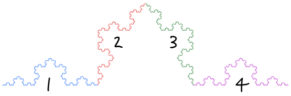
(a) $\ell=1$ decomposition

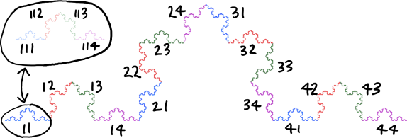
(b) $\ell=2$ decomposition

Figure 3: Level 1 (a) and level 2 (b) decompositions of the Koch curve. To make the labelling more compact, in (a) the labels “$1$”,…,“$4$” indicate the subsets $\Gamma_{1},\ldots,\Gamma_{4}$, and in (b) the labels “$ij$” and “$ijk$” indicate the subsets $\Gamma_{(i,j)}$ and $\Gamma_{(i,j,k)}$. In (b) the insert shows the level 3 decomposition of $\Gamma_{(1,1)}$.

Let $\Gamma\subset\mathbb{R}^{n}$ be the attractor of an IFS $\{s_{1},\ldots,s_{M}\}$ satisfying the OSC, so that $d={\rm dim_{H}}(\Gamma)\in(0,n]$, and recall from §2.1 that $\Gamma$ is a $d$-set. Following [20], for $\ell\in\mathbb{N}$ we define the set of multi-indices $I_{\ell}:=\{1,\ldots,M\}^{\ell}\!=\{{\boldsymbol{m}}=(m_{1},m_{2},\ldots,m_{\ell})$: $\,1\leq m_{j}\leq M,\,j=1,2,\ldots,\ell\}$, and for $E\subset\mathbb{R}^{n}$ and ${\boldsymbol{m}}\in I_{\ell}$ we define $E_{{\boldsymbol{m}}}=s_{m_{1}}\circ s_{m_{2}}\circ\ldots\circ s_{m_{\ell}}(E)$. We also set $I_{0}:=\{0\}$ and adopt the convention that $E_{0}:=E$. This notation extends that of (5) where the sets $\Gamma_{1},\ldots,\Gamma_{M}$ were introduced, corresponding to the case $E=\Gamma$ and $\ell=1$ here. We illustrate this for the Koch curve (Example 2.3, Figure 1(e)) in Figure 3. Illustrations for other examples can be found in [16, Figs 1-6].

Let $0<h\leq\operatorname{diam}(\Gamma)$. Define the index set $L_{h}$ by $L_{h}:=\{0\}$ for $h=\operatorname{diam}(\Gamma)$, and by

$$L_{h}:=\big{\{}{\boldsymbol{m}}\in\bigcup_{\ell=1}^{\infty}I_{\ell}:\operatorname{diam}(\Gamma_{{\boldsymbol{m}}})\leq h\text{ and }\operatorname{diam}(\Gamma_{{\boldsymbol{m}}_{-}})>h\big{\}},$$ (12)

for $h<\operatorname{diam}(\Gamma)$, where, for ${\boldsymbol{m}}=(m_{1},\ldots,m_{\ell})$, ${\boldsymbol{m}}_{-}:=(m_{1},...,m_{\ell-1})$ if $\ell\in\mathbb{N}$ with $\ell\geq 2$, and ${\boldsymbol{m}}_{-}:=0$ if $\ell=1$. We then define

$$\mathbb{Y}_{h}:={\rm span}\big{(}\{\chi_{{\boldsymbol{m}}}\}_{{\boldsymbol{m}}\in L_{h}}\big{)},$$ (13)

where $\{\chi_{{\boldsymbol{m}}}\}_{{\boldsymbol{m}}\in L_{h}}$ is the canonical $\mathbb{L}_{2}(\Gamma)$-orthonormal basis for $\mathbb{Y}_{h}$ given by

$$\chi_{{\boldsymbol{m}}}(x):=\begin{cases}\frac{1}{\mathcal{H}^{d}(\Gamma_{{\boldsymbol{m}}})^{1/2}},&x\in\Gamma_{{\boldsymbol{m}}},\\ 0,&\text{otherwise}.\end{cases}$$ (14)

We now introduce a definition concerning the approximability of elements of the trace spaces $\mathbb{H}^{t}(\Gamma)$ by piecewise constant functions.

Definition 2.8.

Given $0<s\leq 1$ we say that $\Gamma$ is piecewise-constant (PWC) $s$-approximable if, for $-s\leq t_{1}<t_{2}\leq 0$, there exists a constant $c>0$ such that

$$\inf_{\Psi_{h}\in\mathbb{Y}_{h}}\|f-\Psi_{h}\|_{\mathbb{H}^{t_{1}}(\Gamma)}\leq c\,h^{t_{2}-t_{1}}\|f\|_{\mathbb{H}^{t_{2}}(\Gamma)},\qquad 0<h\leq\operatorname{diam}(\Gamma),\quad f\in\mathbb{H}^{t_{2}}(\Gamma).$$ (15)

In the proof of [5, Prop. 5.2] we show the following result.

Theorem 2.9.

Let $0<s<1$ and suppose that the piecewise constant wavelet norm $\|\cdot\|_{t}$ defined in [5, Thm 3.1 and Cor. 3.3(iii)] is equivalent to $\|\cdot\|_{\mathbb{H}^{t}(\Gamma)}$ for $-s\leq t\leq 0$. Then $\Gamma$ is PWC-$s$-approximable.

As a corollary of Theorem 2.9, the following result was proved for disjoint IFS attractors (which have $0<d<n$) as [5, Prop. 5.2]; a key step in the proof was the use of results from [20] to prove the norm equivalence in the hypothesis of Theorem 2.9; see [5, Thm 3.1 and Cor. 3.3(iii)]. The results for the cases $d=n$ and $d=n-1$, proved by quite different arguments, are taken from [4].

Theorem 2.10.

If $\Gamma$ is disjoint then $\Gamma$ is PWC-$s$-approximable for $0<s<1$. If $d=n$ or $d=n-1$ and $\Gamma\subset\Gamma_{\infty}$, for some hyperplane $\Gamma_{\infty}\subset\mathbb{R}^{n}$, then $\Gamma$ is PWC-$s$-approximable for $0<s\leq 1$.

The following trivial lemma, which follows since $\mathrm{tr}_{\Gamma}^{*}:\mathbb{H}^{t}(\Gamma)\to H_{\Gamma}^{t-(n-d)/2}$ is a unitary isomorphism for $-1<t<0$, indeed for $-1\leq t\leq 0$ if $d=n$ and $\widetilde{H}{}^{1}(\Gamma^{c})=\accentset{\smash{\raisebox{-0.3014pt}{$\scriptstyle\circ$}}}{H}\rule{0.0pt}{9.90276pt}{}^{1}(\Gamma^{c})$ (see §2.2), rephrases the notion of PWC-$s$-approximability in the setting of subspaces of $H^{-1}_{\Gamma}$. Here, and henceforth, we define

$$Y_{h}:=\mathrm{tr}_{\Gamma}^{*}(\mathbb{Y}_{h})\subset H^{-1}_{\Gamma}.$$ (16)

Lemma 2.11.

Suppose that $\Gamma$ is PWC-$s$-approximable for some $0<s<1$. Then for $-s-(n-d)/2\leq s_{1}<s_{2}<-(n-d)/2$ there exists a constant $c>0$ such that

$$\inf_{\psi_{h}\in Y_{h}}\|\psi-\psi_{h}\|_{H^{s_{1}}_{\Gamma}}\leq ch^{s_{2}-s_{1}}\|\psi\|_{H^{s_{2}}_{\Gamma}},\qquad 0<h\leq\operatorname{diam}(\Gamma),\quad\psi\in H^{s_{2}}_{\Gamma}.$$ (17)

If $d=n$, $\Gamma$ is PWC-$1$-approximable, and $\widetilde{H}{}^{1}(\Gamma^{c})=\accentset{\smash{\raisebox{-0.3014pt}{$\scriptstyle\circ$}}}{H}\rule{0.0pt}{9.90276pt}{}^{1}(\Gamma^{c})$, then (17) holds for the extended range $-1\leq s_{1}<s_{2}\leq 0$.

3 BVPs and IEs

Let $\Gamma\subset\mathbb{R}^{n}$ be non-empty and compact and let $k>0$. Consider time-harmonic acoustic scattering of an incident wave $u^{i}$ by $\Gamma$, a sound-soft obstacle. We assume that the incident wave $u^{i}$ is an element of $W^{1,{\rm loc}}(\mathbb{R}^{n})=H^{1,{\rm loc}}(\mathbb{R}^{n})$ satisfying the Helmholtz equation

$$\Delta u+k^{2}u=0$$ (18)

in a distributional sense in some neighbourhood of $\Gamma$ (so that $u^{i}$ is $C^{\infty}$ in that neighbourhood by elliptic regularity, see, e.g., [13, Thm 6.3.1.3]); for instance, $u^{i}$ might be the plane wave $u^{i}(x)={\mathrm{e}}^{{\mathrm{i}}k\vartheta\cdot x}$ for some $\vartheta\in\mathbb{R}^{n}$ with $|\vartheta|=1$). Where $\Omega:=\Gamma^{c}=\mathbb{R}^{n}\setminus\Gamma$, we seek a scattered field $u\in W^{1,{\rm loc}}(\Omega)$ satisfying (18) in a distributional sense in $\Omega$ (so that $u\in C^{\infty}(\Omega)$ by elliptic regularity), the Sommerfeld radiation condition

$$\dfrac{\partial{u(x)}}{\partial{r}}-{\mathrm{i}}ku(x)=o(r^{-(n-1)/2}),\qquad r:=|x|\to\infty,\text{ uniformly in }\hat{x}:=x/|x|,$$ (19)

and the boundary condition $u=-u^{i}$ on $\partial\Omega=\partial\Gamma$, enforced by requiring that the total field

$$u^{t}:=u+u^{i}\in W^{1,{\rm loc}}_{0}(\Omega).$$ (20)

This problem, which we will refer to as our scattering problem, is a standard, uniquely-solvable scattering problem in the case that $\Omega$ is connected (see, e.g. [11, §3]). Figure 1, with the exception of (b), and Figure 2 are all examples of such cases. But, to understand the well-posedness of our IE formulation, we also want to allow cases (such as Figure 1(b)) where $\Omega$ is not connected, in which case $\Omega=\Omega_{+}\cup\Omega_{-}$, where $\Omega_{\pm}$ are disjoint open sets, with $\Omega_{+}$ the unbounded component of $\Omega$ and $\Omega_{-}$ a bounded open set. In such cases the above problem decouples into a uniquely-solvable scattering problem for $u|_{\Omega_{+}}\in W^{1,{\rm loc}}(\Omega_{+})$ and the homogeneous Dirichlet problem that $u^{t}|_{\Omega_{-}}\in W_{0}^{1}(\Omega_{-})$ satisfies (18) in $\Omega_{-}$. Thus our scattering problem is uniquely solvable (with $u^{t}=0$ and $u=-u^{i}$ in $\Omega_{-}$) if and only if $k^{2}$ is not a Dirichlet eigenvalue of $-\Delta$ in $\Omega_{-}$. We will frequently assume that $k$ is not one of these exceptional values, making the following assumption.

Assumption 3.1.

$\Gamma\subset\mathbb{R}^{n}$ and $k>0$ are such that, if $v\in W^{1,{\rm loc}}_{0}(\Omega)$ satisfies (18) in $\Omega$ and (19), then $v=0$.

Remark 3.2.

We emphasise that Assumption 3.1 holds for all $k>0$ if $\Omega$ is connected, and that if $\Omega$ is not connected, in which case $\Omega=\Omega_{+}\cup\Omega_{-}$, where $\Omega_{\pm}$ are the disjoint open sets defined above, then Assumption 3.1 holds if and only if there is no non-trivial $v\in W_{0}^{1}(\Omega_{-})$ that satisfies (18) in $\Omega_{-}$, which holds for all $k>0$ outside a countable set whose only accumulation point is infinity.

Under Assumption 3.1, where $u$ is the unique solution to the above scattering problem, it is convenient to extend the definition of $u$ from $\Omega$ to the whole of $\mathbb{R}^{n}$ by setting $u=-u^{i}$ on $\Gamma$. With this extended definition, which we will assume hereafter, $u^{t}=u+u^{i}=0$ on $\Gamma$ so that, by (20), $u^{t}\in\widetilde{H}^{1,{\rm loc}}(\Omega)\subset H^{1,{\rm loc}}(\mathbb{R}^{n})$, so that also $u=u^{t}-u^{i}\in H^{1,{\rm loc}}(\mathbb{R}^{n})$. Alternatively, one can require from the outset that $u\in H^{1,{\rm loc}}(\mathbb{R}^{n})$ and satisfies (18) in $\Omega$ and (19) and that $u^{t}=u+u^{i}\in\widetilde{H}^{1,{\rm loc}}(\Omega)$, in which case $u|_{\Omega}$ is the unique solution to the above scattering problem and $u=-u^{i}$ on $\Gamma$ (almost everywhere with respect to $n$-dimensional Lebesgue measure).

Introducing the orthogonal projection operator

$$P:H^{1}(\mathbb{R}^{n})\to\widetilde{H}{}^{1}(\Omega)^{\perp},$$ (21)

we observe that $u^{t}\in\widetilde{H}^{1,{\rm loc}}(\Omega)$ if and only if $P(\sigma u^{t})=0$ for some, and hence every, $\sigma\in C^{\infty}_{0,\Gamma}$, in other words, if and only if

$$P(\sigma u) =g,$$ (22)

where

$$g:=-P(\sigma u^{i}).$$ (23)

Thus (22) is an alternative formulation of the boundary condition that $u=-u^{i}$ on $\Gamma$, equivalent to the requirement that $u^{t}\in\widetilde{H}^{1,{\rm loc}}(\Omega)$.

We now reformulate our BVP, which is to find $u\in H^{1,{\rm loc}}(\mathbb{R}^{n})$ that satisfies (18) in $\Omega$, (19), and the boundary condition (22), as an IE. In what follows, $\mathcal{A}$ will denote the standard acoustic Newton potential operator, defined for compactly supported $\phi\in L_{2}(\mathbb{R}^{n})=H^{0}(\mathbb{R}^{n})$ by

$$\mathcal{A}\phi(x)=\int_{\mathbb{R}^{n}}\Phi(x,y)\phi(y)\,\mathrm{d}y,\qquad x\in\mathbb{R}^{n},$$ (24)

where $\Phi$ is the Helmholtz fundamental solution defined below (2). It is standard (see e.g. [28, Thm 3.1.2]) that, for $s\in\mathbb{R}$, in particular for $s=0$, $\mathcal{A}$ is continuous as a mapping

$$\mathcal{A}:H^{s-1}_{\rm comp}(\mathbb{R}^{n})\to H^{s+1,{\rm loc}}(\mathbb{R}^{n}),$$ (25)

where, for $s\in\mathbb{R}$, $H^{s}_{\rm comp}(\mathbb{R}^{n})$ is the space of compactly supported elements of $H^{s}(\mathbb{R}^{n})$, and that (e.g. [28, Thm 3.1.4])

$$(\Delta+k^{2})\mathcal{A}\phi=\mathcal{A}(\Delta+k^{2})\phi=-\phi,\qquad\phi\in H^{-1}_{\rm comp}(\mathbb{R}^{n}).$$ (26)

Viewing $\mathcal{A}$ as an operator $\mathcal{A}:H^{-1}_{\Gamma}\to H^{1,{\rm loc}}(\mathbb{R}^{n})=W^{1,{\rm loc}}(\mathbb{R}^{n})$, we have that

$$\mathcal{A}\phi(x)=\langle(\sigma\Phi(x,\cdot)),\overline{\phi}\rangle_{H^{1}(\mathbb{R}^{n})\times H^{-1}(\mathbb{R}^{n})},\quad x\in\Omega,$$ (27)

where $\overline{\phi}$ denotes the complex conjugate of $\phi$ and $\sigma$ is any element of $C^{\infty}_{0,\Gamma}$ with $x\not\in\operatorname{supp}{\sigma}$. We define the operator $A:H^{-1}_{\Gamma}\to\widetilde{H}{}^{1}(\Omega)^{\perp}=(H^{-1}_{\Gamma})^{*}$ by

$$A\phi:=P(\sigma\mathcal{A}\phi),\qquad\phi\in H^{-1}_{\Gamma},$$ (28)

with $\sigma\in C^{\infty}_{0,\Gamma}$ arbitrary. We also define the associated sesquilinear form $a(\cdot,\cdot)$ on $H^{-1}_{\Gamma}\times H^{-1}_{\Gamma}$ by

$$a(\phi,\psi):=\langle A\phi,\psi\rangle_{H^{1}(\mathbb{R}^{n})\times H^{-1}(\mathbb{R}^{n})},\qquad\phi,\psi\in H^{-1}_{\Gamma}.$$ (29)

This form is compactly perturbed coercive, meaning that the operator $A:H^{-1}_{\Gamma}\to\widetilde{H}{}^{1}(\Omega)^{\perp}$ is a compact perturbation of a coercive operator (see, e.g., [10, §2.2] for detailed definitions and discussion). The following lemma is a generalisation of [12, Prop. 8.7, 8.8], and our proof is similar.

Lemma 3.3.

The sesquilinear form $a(\cdot,\cdot)$ is continuous and compactly perturbed coercive on $H^{-1}_{\Gamma}\times H^{-1}_{\Gamma}$. Specifically, for some constants $C_{a},\alpha>0$, and some compact sesquilinear form $\tilde{a}(\cdot,\cdot)$,

$$|a(\phi,\psi)|\leq C_{a}\|\phi\|_{H^{-1}_{\Gamma}}\,\|\psi\|_{H^{-1}_{\Gamma}},\quad|a(\phi,\phi)-\tilde{a}(\phi,\phi)|\geq\alpha\|\phi\|_{H^{-1}_{\Gamma}}^{2},\quad\phi,\psi\in H^{-1}_{\Gamma}.$$ (30)

Proof.

Continuity follows immediately from (25). Let us temporarily introduce the notations $\mathcal{A}_{\kappa}$ and $A_{\kappa}$ to denote the operators $\mathcal{A}$ and $A$ with $k$ replaced by some complex wavenumber $\kappa$. To prove that $a(\cdot,\cdot)$ is compactly perturbed coercive, we split the associated operator $A=A_{k}$ as $A_{k}=A_{{\mathrm{i}}}+(A_{k}-A_{{\mathrm{i}}})$, where $A_{\mathrm{i}}$ is the operator with wavenumber $\kappa={\mathrm{i}}$. It is easy to check that for $\phi\in C^{\infty}_{0}(\mathbb{R}^{n})$ the Fourier transform of $\mathcal{A}_{\mathrm{i}}\phi$ is given by $\hat{\phi}(\xi)/(|\xi|^{2}+1)$, which gives that

$$\langle A_{\mathrm{i}}\phi,\phi\rangle_{H^{1}(\mathbb{R}^{n})\times H^{-1}(\mathbb{R}^{n})}=\int_{\mathbb{R}^{n}}\frac{|\hat{\phi}(\xi)|^{2}}{|\xi|^{2}+1}\,\mathrm{d}\xi=\|\phi\|^{2}_{H^{-1}(\mathbb{R}^{n})},\qquad\phi\in H^{-1}_{\Gamma},$$

so that $A_{\mathrm{i}}:H^{-1}_{\Gamma}\to\widetilde{H}{}^{1}(\Omega)^{\perp}$ is coercive with coercivity constant $\alpha=1$. Further, for all $\sigma\in C^{\infty}_{0,\Gamma}$, $A_{k}-A_{\mathrm{i}}=P\sigma(\mathcal{A}_{k}-\mathcal{A}_{\mathrm{i}})$ and, arguing as in [28, Rem. 3.1.3] and [12, Prop. 8.8], $(\mathcal{A}_{k}-\mathcal{A}_{\mathrm{i}}):H_{\Gamma}^{-1}\to H^{3,{\rm loc}}(\mathbb{R}^{n})$ is continuous, so that $\sigma(\mathcal{A}_{k}-\mathcal{A}_{\mathrm{i}}):H_{\Gamma}^{-1}\to H^{1}(\mathbb{R}^{n})$ is compact, which implies that $A_{k}-A_{\mathrm{i}}$ is compact.

∎

The following theorem provides BVP and IE equivalence and well-posedness.

Theorem 3.4.

Suppose that Assumption 3.1 holds. Then $A:H^{-1}_{\Gamma}\to\widetilde{H}{}^{1}(\Omega)^{\perp}$ is invertible. Further, for every $g\in\widetilde{H}{}^{1}(\Omega)^{\perp}$ the BVP defined by (18) in $\Omega$, (19), and (22) has a unique solution $u\in H^{1,{\rm loc}}(\mathbb{R}^{n})$ given by

$$u=\mathcal{A}\phi,$$ (31)

where $\phi\in H^{-1}_{\Gamma}$ is the unique solution of the IE

$$A\phi=g.$$ (32)

If Assumption 3.1 does not hold then $A\phi=0$ has a non-trivial solution $\phi\in H_{\Gamma}^{-1}$.

Proof.

If $\phi\in H^{-1}_{\Gamma}$ satisfies (32) then $u$ given by (31) solves the BVP, by (26) and (28), and the fact that the acoustic Newton potential (24) satisfies (19). Thus if (32) has a solution then the BVP has a solution, and this solution is unique if Assumption 3.1 holds. By Lemma 3.3, $A$ is continuous and compactly perturbed coercive, and hence Fredholm of index zero by Lax-Milgram. Thus to prove $A:H^{-1}_{\Gamma}\to\widetilde{H}{}^{1}(\Omega)^{\perp}$ is invertible, so that (32) has a unique solution, it suffices to prove that $A$ is injective. For this, suppose that $\phi\in H^{-1}_{\Gamma}$ and $A\phi=0$. Then $\mathcal{A}\phi$ satisfies the homogeneous BVP, so, if Assumption 3.1 holds, we have $\mathcal{A}\phi=0$ in $\Omega$. But, for $\sigma\in C^{\infty}_{0,\Gamma}$, we also have $P(\sigma\mathcal{A}\phi)=A\phi=0$, so $\sigma\mathcal{A}\phi\in\widetilde{H}{}^{1}(\Omega)$. Thus, by (7), $\mathcal{A}\phi=\sigma\mathcal{A}\phi=0$ in $\Omega^{c}=\Gamma$, almost everywhere with respect to $n$-dimensional Lebesgue measure. Hence $\mathcal{A}\phi=0$, and by (26) we conclude that $\phi=0$, proving injectivity, and hence invertibility of $A$.

If Assumption 3.1 does not hold then, by Remark 3.2, where $\Omega_{-}$ is as in that remark, there exists a non-zero $v\in\widetilde{H}{}^{1}(\Omega_{-})\subset\widetilde{H}{}^{1}(\Omega)$ such that $\Delta v+k^{2}v=0$ in $\Omega_{-}$. By (26) we have $v=\mathcal{A}\phi$, where $\phi:=-(\Delta+k^{2})v\in H^{-1}_{\partial\Omega_{-}}\subset H^{-1}_{\Gamma}$. Further, for $\sigma\in C^{\infty}_{0,\Gamma}$, $P(\sigma v)=0$ since $\sigma v\in\widetilde{H}{}^{1}(\Omega)$, so $A\phi=P(\sigma\mathcal{A}\phi)=0$, and $\phi\neq 0$ since $\mathcal{A}\phi=v\neq 0$. ∎

Remark 3.5 (The role of the capacity of $\Gamma$).

We make the trivial observation that, if $H_{\Gamma}^{-1}=\{0\}$, then the only solution to (32) is $\phi=0$, so that the scattered field $u=\mathcal{A}\phi=0$; the incident field does not interact with $\Gamma$. Further, $H^{-1}_{\Gamma}\neq\{0\}$ if and only if $\Gamma$ has positive $H^{1}$ capacity (see, e.g. [23, Thm 13.2.2], and for a collection of related results and generalisations, see [18, 9]). This holds if ${\rm dim_{H}}(\Gamma)>n-2$ [18, Thm 2.12], and is equivalent to ${\rm dim_{H}}(\Gamma)>n-2$ if $\Gamma$ is a $d$-set [18, Thm 2.17].

The following proposition concerns the support of the IE solution, and explores when the scattered fields and IE solutions for different scatterers $\Gamma$ coincide. It implies that if Assumption 3.1 holds for a scatterer $\Gamma$, then the corresponding scattered field and IE solution coincide with those for the scatterer $\Omega_{+}^{c}$, where $\Omega_{+}$ is the unbounded component of $\Gamma^{c}$, and moreover that the IE solution $\phi$ is supported in $\partial\Omega_{+}$.

Proposition 3.6.

Let $\Gamma\subset\mathbb{R}^{n}$ be compact and let $\Omega:=\Gamma^{c}$ be connected. Let $u=\mathcal{A}\phi$ be the unique solution of the scattering problem for $\Gamma$, where $\phi\in H_{\Gamma}^{-1}$ is the unique solution of (32), with $g$ given by (23). Then $\phi\in H^{-1}_{\partial\Gamma}$. Suppose further that $\Gamma_{\dagger}$ is compact, with $\partial\Gamma\subset\Gamma_{\dagger}\subset\Gamma$, and that Assumption 3.1 is satisfied by $\Gamma_{\dagger}$, and let $u_{\dagger}=\mathcal{A}\phi_{\dagger}$ be the unique solution of the scattering problem for $\Gamma_{\dagger}$, where $\phi_{\dagger}\in H_{\Gamma_{\dagger}}^{-1}$ is the unique solution of the IE for $\Gamma_{\dagger}$. Then $u_{\dagger}=u$ and $\phi_{\dagger}=\phi\in H^{-1}_{\partial\Gamma}$.

Proof.

Since $\mathcal{A}\phi+u^{i}=u+u^{i}=u^{t}\in\widetilde{H}{}^{1,{\rm loc}}(\Omega)$,

$$0=(\Delta+k^{2})u^{t}=(\Delta+k^{2})\mathcal{A}\phi+(\Delta+k^{2})u^{i}=-\phi\quad\mbox{in}\quad\Gamma^{\circ},$$ (33)

by (26), and since $u^{i}$ satisfies (18) in a neighbourhood of $\Gamma$. Thus $\phi\in H_{\partial\Gamma}^{-1}$. Further, $u^{t}\in\widetilde{H}{}^{1,{\rm loc}}(\Omega)$ implies that $u^{t}=0$, so $u=-u^{i}$, in $\Gamma^{\circ}$. Since $\Omega\subset\Omega_{\dagger}\subset\Omega\cup\Gamma^{\circ}$, where $\Omega_{\dagger}:=\Gamma_{\dagger}^{c}$, and $u^{i}$ satisfies (18) in a neighbourhood of $\Gamma$, it follows that $u^{t}\in\widetilde{H}{}^{1,{\rm loc}}(\Omega_{\dagger})$ and that $u$ satisfies (18) in $\Omega_{\dagger}$. Since $u$ also satisfies (19) it follows from Assumption 3.1 for $\Gamma_{\dagger}$ that $u_{\dagger}=u$. Since $u-u_{\dagger}=\mathcal{A}(\phi-\phi_{\dagger})$, it follows from (26) that $\phi=\phi_{\dagger}$. ∎

Remark 3.7 (Alternative IEs for the same scattering problem).

Consider the case where $\Omega:=\Gamma^{c}$ is connected and $\Gamma^{\circ}$ is non-empty (e.g., as in Figure 1(a) and (g)). By Proposition 3.6 and Remark 3.2, to solve the scattering problem for $\Gamma$ we can solve the IE on $\Gamma_{\dagger}$, for any compact $\Gamma_{\dagger}$ with $\partial\Gamma\subset\Gamma_{\dagger}\subset\Gamma$ provided $k^{2}$ is not a Dirichlet eigenvalue of $-\Delta$ in $\Omega_{-}:=\Gamma\setminus\Gamma_{\dagger}$, in particular if $0<k<k_{0}$ where $k_{0}^{2}$ is the smallest such eigenvalue. Recall from Theorem 3.4 that the IE on $\Gamma_{\dagger}$ is equivalent to requiring that $u^{t}=\mathcal{A}\phi+u^{i}\in\widetilde{H}{}^{1}(\Gamma_{\dagger}^{c})$, i.e. to enforcing $\mathcal{A}\phi=-u^{i}$ on $\Gamma_{\dagger}$.

Since $\phi\in H_{\partial\Gamma}^{-1}$, the choice $\Gamma_{\dagger}=\partial\Gamma$ is natural; with this choice the IE enforces $\mathcal{A}\phi=-u^{i}$ on $\partial\Gamma$. When $\Omega$ is a Lipschitz open set this corresponds, as we discuss in Remark 3.10 below, to the standard single-layer-potential boundary IE (BIE) formulation. But it may be attractive to choose a larger $\Gamma_{\dagger}$, so that $\mathcal{A}\phi=-u^{i}$ is enforced not just on $\partial\Gamma$ but also at points in $\Gamma^{\circ}$. This reduces the size of $\Omega_{-}$ and so increases $k_{0}$, and hence the interval $(0,k_{0})$ in which the IE is uniquely solvable. (This is the rationale behind the CHIEF method and its variants for removing irregular frequencies of BIEs, e.g., [29], [33].) For the largest choice, $\Gamma_{\dagger}=\Gamma$, $\mathcal{A}\phi=-u^{i}$ is enforced on the whole of $\Gamma$, and the IE is uniquely solvable for all $k>0$, but at the cost in computation of discretising the whole of $\Gamma$ rather than $\partial\Gamma$ or some intermediate set.

We explore this further in §5, where we compare computations for the choices $\Gamma_{\dagger}=\Gamma$ and $\Gamma_{\dagger}=\partial\Gamma$ for the particular example of the Koch snowflake (Figure 1(g)) - see the discussion around Figure 7 below.

The IE (32) can be written in variational form as: given $g\in(\widetilde{H}{}^{1}(\Omega))^{\perp}$, find $\phi\in H^{-1}_{\Gamma}$ such that

$$a(\phi,\psi)=\langle g,\psi\rangle_{H^{1}(\mathbb{R}^{n})\times H^{-1}(\mathbb{R}^{n})},\qquad\forall\psi\in H^{-1}_{\Gamma}.$$ (34)

This will be the starting point for our Galerkin discretisation in §4. Having computed $\phi$ by solving a Galerkin discretisation of (34), we will evaluate $u(x)$ at points $x\in\Omega$ using the formula (31). We will also compute the far-field pattern $u^{\infty}\in C^{\infty}(\mathbb{S}^{n-1})$, which satisfies (see, e.g., [6, Eqn. (2.23)], [24, p. 294])

$$u(x)=\frac{{\mathrm{e}}^{{\mathrm{i}}k|x|}}{|x|^{(n-1)/2}}\left(u^{\infty}(\hat{x})+O(|x|^{-1})\right),\quad\mbox{as}\quad|x|\to\infty,$$

uniformly in $\hat{x}:=x/|x|$. Explicitly ([6, Eqn. (2.23)], [24, p. 294]),

$$u^{\infty}(\hat{x})=\langle\sigma\Phi^{\infty}(\hat{x},\cdot),\overline{\phi}\rangle_{H^{1}(\mathbb{R}^{n})\times H^{-1}(\mathbb{R}^{n})},\quad\hat{x}\in\mathbb{S}^{n-1},$$ (35)

where $\sigma$ is any element of $C^{\infty}_{0,\Gamma}$ and $\Phi^{\infty}(\cdot,y)$ is the far-field pattern of $\Phi(\cdot,y)$, for $y\in\mathbb{R}^{n}$, viz.

$$\Phi^{\infty}(\hat{x},y):=\frac{{\mathrm{i}}k^{(n-3)/2}}{2(2\pi{\mathrm{i}})^{(n-1)/2}}\,\exp(-{\mathrm{i}}k\hat{x}\cdot y),\quad\hat{x}\in\mathbb{S}^{n-1},\;y\in\mathbb{R}^{n}.$$ (36)

3.1 The IE on $d$-sets in trace spaces

Suppose now that $\Gamma$ is a compact $d$-set with $n-2<d\leq n$. In this case one can reformulate the IE in the setting of the trace spaces $\mathbb{H}^{t}(\Gamma)$ introduced in §2.2. Let

$$t_{d}:=1-\frac{n-d}{2}\in(0,1].$$ (37)

Then, by (27) and (11), for $\Psi\in\mathbb{L}_{2}(\Gamma)$ the composition of $\mathcal{A}$ with $\mathrm{tr}_{\Gamma}^{*}$ has the following integral representation with respect to Hausdorff measure:

$$\mathcal{A}\mathrm{tr}_{\Gamma}^{*}\Psi(x)=\int_{\Gamma}\Phi(x,y)\Psi(y)\,\mathrm{d}\mathcal{H}^{d}(y),\qquad x\in\Omega.$$ (38)

Furthermore, for $\Psi\in\mathbb{L}_{\infty}(\Gamma)$ this representation can be extended to $x\in\Gamma$.

Proposition 3.8.

Let $\Gamma$ be a compact $d$-set with $n-2<d\leq n$. For every $\Psi\in\mathbb{L}_{\infty}(\Gamma)$ the right-hand side of (38) is well-defined (as a Lebesgue integral with respect to $\mathcal{H}^{d}$ measure) for all $x\in\mathbb{R}^{n}$ and is a continuous function on $\mathbb{R}^{n}$. Further, (38) holds for almost all $x\in\mathbb{R}^{n}$ with respect to $n$-dimensional Lebesgue measure, so that $\mathcal{A}\mathrm{tr}_{\Gamma}^{*}\Psi\in C(\mathbb{R}^{n})$.

Proof.

That the right-hand-side of (38) is well-defined for all $x\in\mathbb{R}^{n}$ and defines a continuous function on $\mathbb{R}^{n}$ follows as in the proof of [5, Prop. 4.5], using the estimates for convolution integrals with respect to $\mathcal{H}^{d}$ measure on $d$-sets in [5, Rem. 2.2]. For $d<n$, in which case $m(\partial\Gamma)=\mathcal{H}^{n}(\Gamma)=0$, we have immediately, from (38), that (38) holds for almost all $x\in\mathbb{R}^{n}$. For $d=n$, when $\Psi\in\mathbb{L}_{\infty}(\Gamma)\subset L_{2}(\mathbb{R}^{n})$, that (38) holds for all $x\in\mathbb{R}^{n}$ is just a special case of (24).∎

Let us define $\mathbb{A}:\mathbb{H}^{-t_{d}}(\Gamma)\to\mathbb{H}^{t_{d}}(\Gamma)$ by

$$\mathbb{A}:=\mathrm{tr}_{\Gamma}\,A\,\mathrm{tr}_{\Gamma}^{*}.$$ (39)

Then, by (29) and (10),

$$\langle\mathbb{A}\Psi,\widetilde{\Psi}\rangle_{\mathbb{H}^{t_{d}}(\Gamma)\times\mathbb{H}^{-t_{d}}(\Gamma)}=a(\mathrm{tr}_{\Gamma}^{*}\Psi,\mathrm{tr}_{\Gamma}^{*}\widetilde{\Psi}),\quad\Psi,\widetilde{\Psi}\in\mathbb{H}^{-t_{d}}(\Gamma),$$ (40)

so that $\mathbb{A}$ is continuous and compactly perturbed coercive, since $A$ is, and since $\mathrm{tr}_{\Gamma}^{*}$ is an isometry with range in $H_{\Gamma}^{-1}$ (see §2.2). Further, recall from §2.2 that $\mathrm{tr}_{\Gamma}:\widetilde{H}{}^{1}(\Omega)^{\perp}\to\mathbb{H}^{t_{d}}(\Gamma)$ and $\mathrm{tr}_{\Gamma}^{*}:\mathbb{H}^{-t_{d}}(\Gamma)\to H^{-1}_{\Gamma}$ are unitary isomorphisms for $n-2<d<n$, and also for $d=n$ provided that $\widetilde{H}{}^{1}(\Omega)=\accentset{\smash{\raisebox{-0.3014pt}{$\scriptstyle\circ$}}}{H}\rule{0.0pt}{9.90276pt}{}^{1}(\Omega)$. Thus, assuming $\widetilde{H}{}^{1}(\Omega)=\accentset{\smash{\raisebox{-0.3014pt}{$\scriptstyle\circ$}}}{H}\rule{0.0pt}{9.90276pt}{}^{1}(\Omega)$ in the case $d=n$, problem (34) can be equivalently stated as: given $g\in\widetilde{H}{}^{1}(\Omega)^{\perp}$, find $\Psi\in\mathbb{H}^{-t_{d}}(\Gamma)$ such that

$$\mathbb{A}\Psi=\mathrm{tr}_{\Gamma}g,$$ (41)

or, equivalently,

$$\langle\mathbb{A}\Psi,\widetilde{\Psi}\rangle_{\mathbb{H}^{t_{d}}(\Gamma)\times\mathbb{H}^{-t_{d}}(\Gamma)}=\langle\mathrm{tr}_{\Gamma}g,\widetilde{\Psi}\rangle_{\mathbb{H}^{t_{d}}(\Gamma)\times\mathbb{H}^{-t_{d}}(\Gamma)},\qquad\widetilde{\Psi}\in\mathbb{H}^{-t_{d}}(\Gamma),$$ (42)

with the solutions of (41)/(42) and (34) related by $\phi=\mathrm{tr}_{\Gamma}^{*}\Psi$. Further, by Theorem 3.4, both $A:H_{\Gamma}^{-1}\to\widetilde{H}{}^{1}(\Omega)^{\perp}$ and $\mathbb{A}:\mathbb{H}^{-t_{d}}(\Gamma)\to\mathbb{H}^{t_{d}}(\Gamma)$ are invertible under Assumption 3.1. A schematic showing the relationships between the above function spaces and operators is given in Figure 4.

Figure 4: Schema of relevant function spaces and operators for $s=1$, $t=t_{d}:=1-\frac{n-d}{2}$. The operators $\mathrm{tr}_{\Gamma}$ and $\mathrm{tr}_{\Gamma}^{*}$ are isometries, indeed unitary isomorphisms for $n-2<d<n$, and for $d=n$ if $\widetilde{H}{}^{1}(\Gamma^{c})=\accentset{\smash{\raisebox{-0.3014pt}{$\scriptstyle\circ$}}}{H}\rule{0.0pt}{9.90276pt}{}^{1}(\Gamma^{c})$.

Since $\widetilde{H}{}^{1}(\Omega)\subset\ker(\mathrm{tr}_{\Gamma})$ (with equality if $d<n$, see §2.2), we have $\mathrm{tr}_{\Gamma}P\phi=\mathrm{tr}_{\Gamma}\phi$, $\phi\in H^{1}(\mathbb{R}^{n})$. Then, recalling (21) and (28), we see that, with $\sigma\in C^{\infty}_{0,\Gamma}$ arbitrary,

$$\mathbb{A}\Psi=\mathrm{tr}_{\Gamma}(\sigma\mathcal{A}\mathrm{tr}_{\Gamma}^{*}\Psi),\quad\Psi\in\mathbb{H}^{-t_{d}}(\Gamma).$$ (43)

The following integral representation for $\mathbb{A}$ (cf. [5, Thm 4.6]) will be crucial for our Hausdorff IE method in §4.

Theorem 3.9.

Let $\Gamma$ be a compact $d$-set with $n-2<d\leq n$. For $\Psi$ in $\mathbb{L}_{\infty}(\Gamma)$,

$$\mathbb{A}\Psi(x)=\int_{\Gamma}\Phi(x,y)\Psi(y)\mathrm{d}\mathcal{H}^{d}(y),\qquad\text{ for }\mathcal{H}^{d}\text{-a.e.\ }x\in\Gamma.$$ (44)

Proof.

Suppose $\Psi\in\mathbb{L}_{\infty}(\Gamma)$. For $x\in\mathbb{R}^{n}$ let $G(x)$ denote the right-hand side of (38). By Proposition 3.8 and (25), $\sigma G\in H^{1}(\mathbb{R}^{n})$ and is continuous, for $\sigma\in C^{\infty}_{0,\Gamma}$, so that $\mathrm{tr}_{\Gamma}(\sigma G)=(\sigma G)|_{\Gamma}=G|_{\Gamma}$. Since $\mathcal{A}\mathrm{tr}_{\Gamma}^{*}\Psi(x)=G(x)$, for a.e. $x\in\mathbb{R}^{n}$ with respect to $n$-dimensional Lebesgue measure by Proposition 3.8, it follows that $\mathbb{A}\Psi=G|_{\Gamma}$ in $\mathbb{L}_{2}(\Gamma)$, giving the claimed result. ∎

Our next remark builds on the characterisations of the spaces $\mathbb{H}^{t}(\Gamma)$ in Remark 2.7.

Remark 3.10 (Connection to known cases: II).

Our IE (41) is familiar in a number of cases, in each of which $\Gamma$ is a $d$-set by Remark 2.7.

1. If $\Gamma$ is the boundary of a bounded Lipschitz open set (e.g., Figure 1(b)), then $d=n-1$ and $\mathcal{H}^{d}$ coincides with surface measure on $\Gamma$ [14, Theorem 3.8]. Thus the expression (38) for $\mathcal{A}\mathrm{tr}_{\Gamma}^{*}\Psi$ coincides with the definition, e.g., in [6, Eqn. (2.19)], of the standard single-layer potential with density $\Psi$; the representation (44) for $\mathbb{A}$, recalling Remark 2.7(b), coincides with the definition [6, Eqn. (2.32)] of the single-layer potential operator $S:H^{-1/2}(\Gamma)\to H^{1/2}(\Gamma)$; and the IE (41) coincides with [6, Eqn. (2.63)].

2. If the $d$-set $\Gamma$ is a compact subset of $\Gamma_{\infty}$ (our notation as in Remark 2.7(c)), so $\Gamma$ is a planar screen (examples are Figure 1(c) and (e)), the expression (38) for $\mathcal{A}\mathrm{tr}_{\Gamma}^{*}\Psi$ coincides with [5, Eqn. (45)] and the representation (44) for $\mathbb{A}$ coincides with [5, Eqn. (51)].

3. In the case where $\Gamma$ is a multi-screen, the representation (38) for $\mathcal{A}\mathrm{tr}_{\Gamma}^{*}$ coincides with the definition of the single-layer potential given in [12, Eqn. (8.2)] and the representation (44) for $\mathbb{A}$ coincides with the first boundary integral operator from Proposition 8.8 in [12]. The mapping properties and coercivity property up to compact perturbation derived in Lemma 3.3 generalize the first inequality of [12, Prop. 8.8].

The definition and mapping properties of $\mathrm{tr}_{\Gamma}$ and $\mathrm{tr}_{\Gamma}^{*}$, noted in §2.2, combined with the representation (43), enable us to extend the domain of $\mathbb{A}$ to $\mathbb{H}^{-t}(\Gamma)$, for $t_{d}<t<2t_{d}$, or restrict it to $\mathbb{H}^{-t}(\Gamma)$, for $0<t<t_{d}$, as stated in the following result (cf. [5, Prop. 4.7]).

Proposition 3.11.

Let $\Gamma$ be a compact $d$-set with $n-2<d\leq n$. For $|t|<t_{d}$, $\mathbb{A}:\mathbb{H}^{t-t_{d}}(\Gamma)\to\mathbb{H}^{t+t_{d}}(\Gamma)$ and is continuous. When $d=n$ this holds also for $t=\pm t_{d}=\pm 1$.

Proof.

This follows from (43) and the mapping properties (25) of $\mathcal{A}$, recalling from §2.2 that, for $s>(n-d)/2$, the mappings $\mathrm{tr}_{\Gamma}:H^{s}(\mathbb{R}^{n})\to\mathbb{H}^{t}(\Gamma)$ and $\mathrm{tr}_{\Gamma}^{*}:\mathbb{H}^{-t}(\Gamma)\to H_{\Gamma}^{-s}$ are continuous, where $t=s-(n-d)/2>0$, and that, when $d=n$ and $t=s$, these mappings are continuous also for $s=0$. ∎

In the case that $\Gamma$ is an IFS attractor satisfying the OSC and $d={\rm dim_{H}}(\Gamma)=n$ or $\Gamma$ is disjoint (in which case $d<n$), we can prove additionally that $\mathbb{A}:\mathbb{H}^{t-t_{d}}(\Gamma)\to\mathbb{H}^{t+t_{d}}(\Gamma)$ is invertible for a range of $t$.

Proposition 3.12.

Let $\Gamma$ be an IFS attractor satisfying the OSC and suppose that $d={\rm dim_{H}}(\Gamma)=n$ or that $\Gamma$ is disjoint with $n-2<d<n$. Then there exists $0<\epsilon\leq t_{d}$ such that, provided Assumption 3.1 holds, $\mathbb{A}:\mathbb{H}^{t-t_{d}}(\Gamma)\to\mathbb{H}^{t+t_{d}}(\Gamma)$ is invertible for $|t|<\epsilon$.

Proof.

The claimed invertibility of $\mathbb{A}:\mathbb{H}^{t-t_{d}}(\Gamma)\to\mathbb{H}^{t+t_{d}}(\Gamma)$ for a range of $t$ in a neighbourhood of $t=0$ follows by applying a result on interpolation of invertibility of operators ([25, Prop. 4.7], which quotes [30]), recalling that (i) $\mathbb{A}:\mathbb{H}^{t-t_{d}}(\Gamma)\to\mathbb{H}^{t+t_{d}}(\Gamma)$ is bounded for $|t|<t_{d}$ (Proposition 3.11); (ii) $\mathbb{A}:\mathbb{H}^{-t_{d}}(\Gamma)\to\mathbb{H}^{t_{d}}(\Gamma)$ is invertible, as noted below (42); and (iii) in the case that $\Gamma$ is disjoint and $d<n$, $\{\mathbb{H}^{t}(\Gamma)\}_{|t|<1}$ is an interpolation scale [5, Cor. 3.3]; (iv) in the case that $d=n$, $\{\mathbb{H}^{t}(\Gamma)\}_{t\geq 0}$ and $\{\mathbb{H}^{t}(\Gamma)\}_{t\leq 0}$ are interpolation scales [4]. ∎

Remark 3.13 (The largest $\epsilon$ for which Proposition 3.11 holds).

A natural conjecture is that, to match Proposition 3.11, the above proposition holds with $\epsilon=t_{d}$ and for every $d$-set (cf. [5, Conj. 4.8]). But such a conjecture must fail in cases where $d^{\prime}:={\rm dim_{H}}(\partial\Omega_{+})<d$, where $\Omega_{+}$ is the unbounded component of $\Omega=\Gamma^{c}$. (Figure 1(a) and (g) are such cases, with $d^{\prime}=1$ for (a), $d^{\prime}=\log(4)/\log(3)$ for (g), $d=2$ for (a) and (g).) For, given that $\mathrm{tr}_{\Gamma}g=-u^{i}|_{\Gamma}\in\mathbb{H}^{t}(\Gamma)$ for every $t>0$, and where $\Psi$ and $\phi=\mathrm{tr}_{\Gamma}^{*}\Psi$ denote the solutions of (41) and (32), respectively, such a conjecture would imply that $\Psi\in\mathbb{H}^{t}(\Gamma)$ for every $t<0$, so that, for every $s<-(n-d)/2$, $\phi\in H_{\Gamma}^{s}$, indeed $\phi\in H_{\partial\Omega_{+}}^{s}$, since $\phi$ is supported in $\partial\Omega_{+}$ by Proposition 3.6. But, if $u_{i}|_{\Gamma}\neq 0$, so $\Psi\neq 0$ and $\phi\neq 0$, it is impossible that $\phi\in H_{\partial\Omega_{+}}^{s}$ for $s>-(n-d^{\prime})/2$, since then $H^{s}_{\partial\Omega_{+}}=\{0\}$ [18, Thm. 2.12], indeed $H^{s}_{\partial\Omega_{+}}=\{0\}$ if and only if $s\geq-(n-d^{\prime})/2$ if $\partial\Omega_{+}$ is a $d^{\prime}$-set.

A plausible modified conjecture, in cases where $\Gamma$ is a $d$-set and $\Omega_{+}$ is a $d^{\prime}$-set, is that the above proposition holds with $\epsilon=t_{d^{\prime}}$. (Note that the examples in Figures 1 and 2 are all $d$-sets with the indicated values of $d$, and, in each case, $\partial\Omega_{+}$ is a $d^{\prime}$-set, with $d^{\prime}=d$ (since $\partial\Omega_{+}=\partial\Gamma$) except for Figure 1(a) and (g) where the $d^{\prime}$ values are as stated above.) We will provide in §5 numerical results which will suggest that this conjecture holds in cases that $d^{\prime}<n-1$ but not in cases that $d^{\prime}>n-1$.

Remark 3.14 (Solution regularity in the $H_{\Gamma}^{s}$ scale).

The mapping properties of $\mathrm{tr}_{\Gamma}^{*}$ recalled in §2.2, combined with (39), imply that if, for some $0<t<t_{d}$, $\mathbb{A}:\mathbb{H}^{t-t_{d}}(\Gamma)\to\mathbb{H}^{t+t_{d}}(\Gamma)$ is invertible, if $\mathrm{tr}_{\Gamma}g\in\mathbb{H}^{t+t_{d}}(\Gamma)$, and if $\widetilde{H}{}^{1}(\Omega)=\accentset{\smash{\raisebox{-0.3014pt}{$\scriptstyle\circ$}}}{H}\rule{0.0pt}{9.90276pt}{}^{1}(\Omega)$ in the case $d=n$, then the solution $\phi=\mathrm{tr}_{\Gamma}^{*}\Psi$ of the IE (32) satisfies

$$\phi\in H^{-1+t}_{\Gamma},\quad\mbox{with}\quad\|\phi\|_{H^{-1+t}_{\Gamma}}\leq C\|\mathrm{tr}_{\Gamma}g\|_{\mathbb{H}^{t+t_{d}}(\Gamma)},$$ (45)

for some constant $C>0$ independent of $\phi$ and $g$. In the case of scattering of an incident wave $u^{i}$, in which $g$ is given by (23), we have that $\mathrm{tr}_{\Gamma}g=-u^{i}|_{\Gamma}\in\mathbb{H}^{t+t_{d}}(\Gamma)$ for all $0<t<t_{d}$, since $u^{i}$ is $C^{\infty}$ in a neighbourhood of $\Gamma$. Hence, in this case, if $\Gamma$ is an IFS attractor satisfying the OSC and either $d=n$ or $\Gamma$ is disjoint and $n-2<d={\rm dim_{H}}(\Gamma)<n$, then, by Proposition 3.12, (45) holds for $0<t<\epsilon$, where $\epsilon$ is as in Proposition 3.12. Thus, if Proposition 3.12 holds with $\epsilon=t_{d^{\prime}}$, where $d^{\prime}$ is as in the above remark, then (45) applies for $0<t<t_{d^{\prime}}$.

4 The Hausdorff-measure IEM

We now define and analyse our Hausdorff-measure Galerkin IEM. To begin with, let us assume that $\Gamma$ is a compact $d$-set for some $n-2<d\leq n$. Given $N\in\mathbb{N}$ let $\{T_{j}\}_{j=1}^{N}$ be a mesh of $\Gamma$, a collection of $\mathcal{H}^{d}$-measurable subsets of $\Gamma$ (the elements) such that

$$\Gamma=\bigcup_{j=1}^{N}T_{j},\quad\mathcal{H}^{d}(T_{j})>0\text{ for }j=1,\ldots,N,\quad\text{ and }\mathcal{H}^{d}(T_{j}\cap T_{j^{\prime}})=0\text{ for }j\neq j^{\prime},$$

and set $h:=\max_{j=1,\ldots,N}\operatorname{diam}(T_{j})$. Define the $N$-dimensional space of piecewise constants

$$\mathbb{V}_{N}:=\{f\in\mathbb{L}_{2}(\Gamma):f|_{T_{j}}=c_{j}\text{ for some }c_{j}\in\mathbb{C},\,j=1,\ldots,N\}\subset\mathbb{L}_{2}(\Gamma)$$ (46)

and set

$$V_{N}:=\mathrm{tr}_{\Gamma}^{*}(\mathbb{V}_{N})\subset H^{-1}_{\Gamma}.$$ (47)

Suppose now that $h\to 0$ as $N\to\infty$. Then it is easy to see that

$$\inf_{f_{N}\in{\mathbb{V}}_{N}}\|f-f_{N}\|_{{\mathbb{L}}_{2}(\Gamma)}\to 0$$

as $N\to\infty$ for every $f\in\mathbb{L}_{2}(\Gamma)$. Thus (cf. [5, Thm 5.1])

$$\inf_{\psi_{N}\in V_{N}}\|\psi-\psi_{N}\|_{H^{-1}(\mathbb{R}^{n})}\to 0\quad\mbox{as}\quad N\to\infty,\quad\mbox{for all}\quad\psi\in H_{\Gamma}^{-1},$$ (48)

if and only if $\mathrm{tr}_{\Gamma}^{*}(\mathbb{L}_{2}(\Gamma))$ is dense in $H_{\Gamma}^{-1}$. By the results of §2.2, this density result holds if $n-2<d<n$, and holds also in the case $d=n$ if and only if $\widetilde{H}{}^{1}(\Gamma^{c})=\accentset{\smash{\raisebox{-0.3014pt}{$\scriptstyle\circ$}}}{H}\rule{0.0pt}{9.90276pt}{}^{1}(\Gamma^{c})$.

Our method for solving the IE (32) uses $V_{N}$ as the approximation space in a Galerkin method, based on (34), with $a$ defined by (29). Given $g\in(\widetilde{H}{}^{1}(\Gamma^{c}))^{\perp}$ we seek $\phi_{N}\in V_{N}$ such that

$$a(\phi_{N},\psi_{N})=\langle g,\psi_{N}\rangle_{H^{1}(\mathbb{R}^{n})\times H^{-1}(\mathbb{R}^{n})},\qquad\forall\psi_{N}\in V_{N}.$$ (49)

Let $\{f^{i}\}_{i=1}^{N}$ be a basis for $\mathbb{V}_{N}$, and let $\{e^{i}=\mathrm{tr}_{\Gamma}^{*}f^{i}\}_{i=1}^{N}$ be the corresponding basis for $V_{N}$. Then, writing $\phi_{N}=\sum_{j=1}^{N}c_{j}e^{j}$, (49) implies that $\vec{c}=(c_{1},\ldots,c_{N})^{T}\in\mathbb{C}^{N}$ satisfies the system

$$\underline{\underline{A}}\vec{c}=\vec{b},$$ (50)

where, by (40), (9), and (44), the matrix $\underline{\underline{A}}\in\mathbb{C}^{N\times N}$ has $(i,j)$-entry given by

$$A_{ij}=a(e^{j},e^{i}) =\langle\mathbb{A}f^{j},f^{i}\rangle_{\mathbb{H}^{t_{d}}(\Gamma)\times\mathbb{H}^{-t_{d}}(\Gamma)}$$

$$=\int_{\Gamma}\int_{\Gamma}\Phi(x,y)f^{j}(y)\overline{f^{i}(x)}\,\mathrm{d}\mathcal{H}^{d}(y)\mathrm{d}\mathcal{H}^{d}(x),$$ (51)

and, by (11), the vector $\vec{b}\in\mathbb{C}^{N}$ has $i$th entry given by

$$b_{i}=\langle g,e^{i}\rangle_{H^{1}(\mathbb{R}^{n})\times H^{-1}(\mathbb{R}^{n})}=\int_{\Gamma}\mathrm{tr}_{\Gamma}g(x)\overline{f^{i}(x)}\,\mathrm{d}\mathcal{H}^{d}(x),$$ (52)

with $\mathrm{tr}_{\Gamma}g(x)=-u^{i}(x)$, $x\in\Gamma$, for the scattering problem with $g$ given by (23). (For a more detailed derivation of these formulas see the analogous calculations in [5, §5], noting that in the case that $\Gamma$ is a planar screen in the sense of Remarks 2.7 and 3.10 the above Galerkin method is identical to that proposed in [5, §5] and the linear system (50) is identical to [5, Eqn. (57)].)

Once we have computed $\phi_{N}$ by solving (50) we will compute approximations to $u(x)$ and $u^{\infty}(x)$, given by (31)/(27) and (35), respectively. Each expression takes the form $J(\phi)$, where

$$J(\psi):=\langle\varphi,\overline{\psi}\rangle_{H^{1}(\mathbb{R}^{n})\times H^{-1}(\mathbb{R}^{n})},\quad\psi\in H^{-1}_{\Gamma},$$ (53)

for some $\varphi\in(\widetilde{H}{}^{1}(\Omega))^{\perp}$. Explicitly,

$$\varphi=P\left(\sigma v\right),$$ (54)

where $\sigma$ is any element of $C^{\infty}_{0,\Gamma}$ (with $x$ not in the support of $\sigma$ in the case that $J(\phi)=u(x)$) and $v=\Phi(x,\cdot)$ in the case that $J(\phi)=u(x)$, $v=\Phi^{\infty}(\hat{x},\cdot)$ in the case that $J(\phi)=u^{\infty}(\hat{x})$; note that each $v$ is $C^{\infty}$ in a neighbourhood of $\Gamma$. In each case we approximate $J(\phi)$ by $J(\phi_{N})$ which, recalling (11), is given explicitly by (cf. [5, Eqn. (64)])

$$J(\phi_{N})=\langle\varphi,\overline{\phi_{N}}\rangle_{H^{1}(\mathbb{R}^{n})\times H^{-1}(\mathbb{R}^{n})}=\vec{c}^{T}\vec{\varphi},$$ (55)

where $\vec{\varphi}$ has $j$th entry given by

$$\vec{\varphi}_{j}=\int_{\Gamma}\mathrm{tr}_{\Gamma}\varphi(x)\,f^{j}(x)\,\mathrm{d}\mathcal{H}^{d}(x),$$ (56)

and $\mathrm{tr}_{\Gamma}\varphi(x)=v(x)$, $x\in\Gamma$, for $\varphi$ given by (54). The following is a basic convergence result.

Theorem 4.1.

Let $\Gamma$ be a compact $d$-set for some $n-2<d\leq n$, with $\widetilde{H}{}^{1}(\Gamma^{c})=\accentset{\smash{\raisebox{-0.3014pt}{$\scriptstyle\circ$}}}{H}\rule{0.0pt}{9.90276pt}{}^{1}(\Gamma^{c})$ in the case $d=n$. Suppose that Assumption 3.1 holds, and that $h\to 0$ as $N\to\infty$. Then for all sufficiently large $N\in\mathbb{N}$ the variational problem (49) has a unique solution $\phi_{N}\in V_{N}$ that is quasi-optimal in the sense that, for some constant $C>0$ independent of $\phi$ and $N$,

$$\|\phi-\phi_{N}\|_{H^{-1}(\mathbb{R}^{n})}\leq C\inf_{\psi_{N}\in V_{N}}\|\phi-\psi_{N}\|_{H^{-1}(\mathbb{R}^{n})},$$ (57)

where $\phi\in H^{-1}_{\Gamma}$ denotes the solution of (32). Furthermore, $\|\phi-\phi_{N}\|_{H^{-1}(\mathbb{R}^{n})}\to 0$ as $N\to\infty$, and, where $J(\cdot)$ is given by (53) for some $\varphi\in(\widetilde{H}{}^{1}(\Omega))^{\perp}$, $J(\phi_{N})\to J(\phi)$ as $N\to\infty$.

Proof.

The sesquilinear form $a(\cdot,\cdot)$ is compactly perturbed coercive (Lemma 3.3), and invertible if Assumption 3.1 holds (Theorem 3.4), so the quasi-optimality (57) holds for all sufficiently large $N$ by (48) and standard Galerkin method theory [28, §4.2.3]. The remaining results follow by (48) and the continuity of the linear functional $J(\cdot)$. ∎

4.1 Galerkin error estimates

We now assume that $\Gamma$ is the attractor of an IFS satisfying the OSC, as in §2.1. In this case $\widetilde{H}{}^{1}(\Gamma^{c})=\accentset{\smash{\raisebox{-0.3014pt}{$\scriptstyle\circ$}}}{H}\rule{0.0pt}{9.90276pt}{}^{1}(\Gamma^{c})$ (see §2.2) and, given $0<h\leq\operatorname{diam}{\Gamma}$, we can take $\{T_{j}\}_{j=1}^{N}=\{\Gamma_{{\boldsymbol{m}}}\}_{{\boldsymbol{m}}\in L_{h}}$, where $L_{h}$ was defined in (12), so that $V_{N}=Y_{h}$, where $Y_{h}$ was defined in (16).

Combining the asymptotic quasi-optimality result (57) with the best approximation error estimates from §2.3 gives an error bound for the Galerkin approximation provided that $\phi$ is sufficiently smooth. By Theorem 2.10, the assumptions of the following theorem on the attractor $\Gamma$ hold if $d=n$, if $d=n-1$ and $\Gamma$ lies in a hyperplane, or if $n-2<d<n$ and $\Gamma$ is disjoint.

Theorem 4.2.

Let $\Gamma$ be a PWC-$s$-approximable IFS attractor with $n-2<d={\rm dim_{H}}(\Gamma)\leq n$ and $s=1-(n-d)/2$. Let $\phi$ be the unique solution of (32) and let $\phi_{N}$ be the unique solution of (49) (defined for all sufficiently large $N$) with $V_{N}=Y_{h}$, with $Y_{h}$ defined as in (16). Suppose that $\phi\in H^{s}_{\Gamma}$ for some $-1<s<-(n-d)/2$. Then, for some constant $c>0$ independent of $h$ and $\phi$,

$$\|\phi-\phi_{N}\|_{H^{-1}_{\Gamma}}\leq ch^{s+1}\|\phi\|_{H^{s}_{\Gamma}},$$ (58)

for all sufficiently large $N$. Furthermore, let $\varphi\in(\widetilde{H}{}^{1}(\Omega))^{\perp}$ be such that the solution $\zeta\in H^{-1}_{\Gamma}$ of (34), with $g$ replaced by $\varphi\in(\widetilde{H}{}^{1}(\Omega))^{\perp}$, also lies in $H^{s}_{\Gamma}$. Then the linear functional $J(\cdot)$ defined by (53) satisfies

$$|J(\phi)-J(\phi_{N})|\leq ch^{2s+2}\|\phi\|_{H^{s}_{\Gamma}}\|\zeta\|_{H^{s}_{\Gamma}},$$ (59)

for some constant $c>0$ independent of $h$, $\phi$, and $\zeta$, for all sufficiently large $N$.

Proof.

The bound (58) is immediate from the quasi-optimality estimate (57) and the definition of PWC-$s$-approximability. The bound (59) follows from (58) by standard Aubin-Nitsche trick arguments – see the proof of [5, Thm 5.6] for more details. ∎

Remark 4.3 (Convergence rates when the IFS is homogeneous).

Suppose that, in addition to the assumptions of Theorem 4.2, $\Gamma$ is homogeneous, with $\rho_{m}=\rho$ for $m=1,\ldots,M$, for some $0<\rho<1$, in which case $d={\rm dim_{H}}(\Gamma)=\log(M)/\log(1/\rho)$, and suppose that $\partial\Omega_{+}$ is a $d^{\prime}$-set, where $\Omega_{+}$ is the unbounded component of $\Omega$, in which case $d^{\prime}\leq d\leq n$, with $d^{\prime}=d$ if $\partial\Omega_{+}=\Gamma$. Suppose that we take $h=\rho^{\ell}\operatorname{diam}{\Gamma}$, so that we use the approximation space $V_{N}=\mathrm{tr}_{\Gamma}^{*}({\rm span}\left(\{\chi_{{\boldsymbol{m}}}\}_{{\boldsymbol{m}}\in I_{\ell}}\right))$, with $I_{\ell}=\{1,\ldots,M\}^{\ell}$. Suppose that we have the maximum possible regularity for $\phi$, i.e., as discussed in Remark 3.13, Proposition 3.12 holds with $\epsilon=t_{d^{\prime}}$, in which case (see Remark 3.14), $\phi\in H^{s}_{\Gamma}$ for every $-1<s<-(n-d^{\prime})/2$ if the datum $g$ is smooth. Then, assuming that the bounds in Theorem 4.2 are sharp, in numerical experiments we should expect to see errors in the computation of $\phi$ and of linear functionals of $\phi$ roughly proportional to $h^{1+(d^{\prime}-n)/2}$ and $h^{2+d^{\prime}-n}$, respectively. In other words, since $h$ is proportional to $\rho^{\ell}$ and $\rho=M^{-1/d}$, we should see errors proportional to $(M^{d^{\prime}/d})^{-\ell/2}$ and $(M^{d^{\prime}/d})^{-\ell}$, respectively, in the case $n=2$, and proportional to $(M^{d^{\prime}/d}\rho)^{-\ell/2}$ and $(M^{d^{\prime}/d}\rho)^{-\ell}$, respectively, in the case $n=3$.

4.2 Numerical quadrature

To implement our method we need suitable numerical quadrature rules to evaluate the integrals (51), (52) and (56). For this we generalise the approach taken for the screen case in [5]. Here we give only the main ideas, and refer the reader to Appendix A, [5, §5.4], and [17, 16] for details.

Suppose that $\Gamma$ is the attractor of an IFS satisfying the OSC, and that, as in §4.1, we are using the approximation space $V_{N}=Y_{h}$ given by (16). Suppose that $g$ is given by (23) and $\varphi$ by (54), with $u^{i}$ and $v$ both $C^{\infty}$ in a neighbourhood of $\mathrm{Hull}(\Gamma)$, the convex hull of $\Gamma$. Suppose that we adopt the canonical $\mathbb{L}_{2}(\Gamma)$-normalised basis (14), so that $f^{j}=\chi_{{\boldsymbol{m}}(j)}$, $j=1,\ldots,N$, where $N:=|L_{h}|$, with $L_{h}$ given by (12), and $({\boldsymbol{m}}(1),\ldots,{\boldsymbol{m}}(N))$ is some ordering of the elements of $L_{h}$. Then, where $\mu_{{\boldsymbol{m}}}:=\mathcal{H}^{d}(\Gamma_{\boldsymbol{m}})$ for ${\boldsymbol{m}}\in L_{h}$, the integrals to be evaluated are, for $i,j\in\{1,\ldots,N\}$,

$$A_{ij} =\mu_{{\boldsymbol{m}}(i)}^{-1/2}\mu_{{\boldsymbol{m}}(j)}^{-1/2}\int_{\Gamma_{{\boldsymbol{m}}(i)}}\int_{\Gamma_{{\boldsymbol{m}}(j)}}\Phi(x,y)\,\mathrm{d}\mathcal{H}^{d}(y)\mathrm{d}\mathcal{H}^{d}(x),$$ (60)

$$b_{i} =-\mu_{{\boldsymbol{m}}(i)}^{-1/2}\int_{\Gamma_{{\boldsymbol{m}}(i)}}u^{i}(x)\,\mathrm{d}\mathcal{H}^{d}(x),\qquad\qquad\vec{\varphi}_{i}=\mu_{{\boldsymbol{m}}(i)}^{-1/2}\int_{\Gamma_{{\boldsymbol{m}}(i)}}v(x)\,\mathrm{d}\mathcal{H}^{d}(x).$$ (61)

Since $u^{i}$ and $v$ are smooth in a neighbourhood of $\Gamma$, (61) can be evaluated using the composite barycentre rule of [17, Defn 3.1], cf. [5, (99)-(101)]. This involves decomposing the mesh element $\Gamma_{{\boldsymbol{m}}(i)}$ into smaller self-similar sub-elements whose vector indices are taken from the index set $L_{h_{Q}}$, for some maximum quadrature element diameter $h_{Q}\leq h$, and applying a one-point quadrature rule on each sub-element. Similarly, provided that $\Gamma_{{\boldsymbol{m}}(i)}$ and $\Gamma_{{\boldsymbol{m}}(j)}$ are disjoint, (60) can be evaluated using a tensor product version of this composite barycentre rule (defined in [17, Defn 3.5]), cf. [5, (94)].

When $\Gamma_{{\boldsymbol{m}}(i)}$ and $\Gamma_{{\boldsymbol{m}}(j)}$ are not disjoint, the integral in (60) is singular. Singularity subtraction reduces the problem to the evaluation of

$$\int_{\Gamma_{{\boldsymbol{m}}(i)}}\int_{\Gamma_{{\boldsymbol{m}}(j)}}\Phi_{\rm sing}(x,y)\,\mathrm{d}\mathcal{H}^{d}(y)\mathrm{d}\mathcal{H}^{d}(x),$$ (62)

where $\Phi_{\rm sing}(x,y)=-\log(|x-y|)/(2\pi)$ if $n=2$, and $\Phi_{\rm sing}(x,y)=1/(4\pi|x-y|)$ if $n=3$. The integral of $\Phi-\Phi_{\rm sing}$ is regular and can be evaluated using the tensor product composite barycentre rule, cf. [5, (96)]. The treatment of (62) depends on the nature of $\Gamma$.

If $\Gamma$ is disjoint (e.g. the Cantor set, Figure 1(e)) then (62) is singular if and only if $i=j$, in which case (62) can be evaluated using the quadrature rules of [17, §4.3], cf. [5, (97)-(98)]. These rules exploit the self-similarity of $\Gamma$ and the homogeneity of $\Phi_{\rm sing}$ to write the singular integral (62) in terms of regular integrals, which can be evaluated by the composite barycentre rule.

If $\Gamma$ is non-disjoint (e.g. the Koch curve, or the Koch snowflake, Fig. 1(f), (g)) then the situation is more complicated, because, in addition to the self-interaction case $i=j$, (62) can also be singular for $i\neq j$, if $\Gamma_{{\boldsymbol{m}}(i)}$ and $\Gamma_{{\boldsymbol{m}}(j)}$ intersect at a point, or at a higher-dimensional set. For certain non-disjoint attractors, it holds that: (i) all singular instances of (62) that arise in our discretization can be written in terms of one of a finite collection of “fundamental” singular integrals, which capture the different singular interactions that can occur between mesh elements; and (ii) these fundamental singular integrals together satisfy a small linear system of equations that can be solved in closed form in terms of regular integrals, which can be evaluated using the composite barycentre rule. A general algorithm for identifying the fundamental singular integrals and deriving the associated linear system was presented in [16, Algorithm 1], along with explicit formulas for the Sierpinski triangle, the Vicsek fractal, the Sierpinski carpet, and the Koch snowflake. These formulas were then applied in the context of screen scattering problems in [16, §7.3]. In Appendix A we briefly explain the methodology of [16], and derive explicit formulas for the case of the Koch curve, which was not considered in [16].

The accuracy of the quadrature approximations described above for the evaluation of (60) and (61) can be controlled by a single parameter $h_{Q}\leq h$, which represents the maximum diameter of the sub-elements used in the composite barycentre rule. Using the results of [17, §4.3] and [16, §6] one can prove quadrature error estimates, which we present in Theorem 4.5 below. In the statement of this theorem we use the following assumption, which guarantees that the singular quadrature rules of [17] and [16] can be applied.

Assumption 4.4.

$\Gamma$ is such that Algorithm 1 from [16] terminates (for the case of Hausdorff measure), producing a finite collection of “fundamental” singular integrals (in the terminology of [17]), and that $\mathrm{Hull}(\Gamma_{\boldsymbol{m}})\cap\mathrm{Hull}(\Gamma_{\boldsymbol{m}^{\prime}})=\emptyset$ for every regular integral $I_{{\boldsymbol{m}},{\boldsymbol{m}^{\prime}}}$ appearing in the vector $\mathbf{r}$ on the right-hand side of the linear system in [16, Eqn (38)], which we assume to be invertible. These assumptions hold in particular if $\Gamma$ is hull-disjoint, meaning that $\mathrm{Hull}(\Gamma_{m})\cap\mathrm{Hull}(\Gamma_{m^{\prime}})=\emptyset$ for every $m,m^{\prime}\in\{1,\ldots,M\}$.

Theorem 4.5.

Let $\Gamma$ be an IFS attractor satisfying the OSC. Let $\underline{\underline{A}}^{Q}$, ${\vec{b}}^{Q}$ and $\vec{\varphi}^{Q}$ denote the approximations of (60) and (61) obtained via the quadrature described above, using a maximum sub-element diameter $0<h_{Q}\leq h$ in the composite barycentre rule.

1. Let $u^{i}$ satisfy the Helmholtz equation in some open neighbourhood of $\mathrm{Hull}(\Gamma)$. Then

   $$\|{\vec{b}}-{\vec{b}}^{Q}\|_{2}\leq h_{Q}^{2}|u^{i}|_{2,\mathrm{Hull}(\Gamma)}\mathcal{H}^{d}(\Gamma)^{1/2},$$ (63)

   where $|u^{i}|_{2,\mathrm{Hull}(\Gamma)}:=\max_{x\in\mathrm{Hull}(\Gamma)}\max_{\begin{subarray}{c}\alpha\in\mathbb{N}_{0}^{n}\\ |\alpha|=2\end{subarray}}|D^{\alpha}u^{i}(x)|$.

2. Let $v$ be $C^{\infty}$ in a neighbourhood of $\mathrm{Hull}(\Gamma)$. Given $\psi_{N}\in V_{N}=Y_{h}$, let $J^{Q}(\psi_{N})$ be defined by (55) with $\vec{\varphi}$ replaced by $\vec{\varphi}^{Q}$, and let $\vec{\psi}$ denote the coefficient vector of $\psi_{N}$ in the basis $\{e^{i}=\mathrm{tr}_{\Gamma}^{*}f^{i}\}_{i=1}^{N}$. Then, there exists $C>0$, independent of $h$, $h_{Q}$, $v$ and $\psi_{N}$, such that

   $$|J(\psi_{N})-J^{Q}(\psi_{N})| \leq h_{Q}^{2}|v|_{2,\mathrm{Hull}(\Gamma)}\|\vec{\psi}\|_{2}\mathcal{H}^{d}(\Gamma)^{1/2}.$$ (64)

3. Let Assumption 4.4 hold. Then there exists $C>0$, independent of $h$ and $h_{Q}$, such that

   $$\|\underline{\underline{A}}-\underline{\underline{A}}^{Q}\|_{2}\leq Ch_{Q}h^{-(n-1)}\mathcal{H}^{d}(\Gamma).$$ (65)

   If, further, $\Gamma$ is homogeneous, then

   $$\|\underline{\underline{A}}-\underline{\underline{A}}^{Q}\|_{2}\leq Ch_{Q}^{2}h^{-n}\mathcal{H}^{d}(\Gamma).$$ (66)

Proof.

Follows that of [5, Thm 5.14], except that, for (iii), if $\Gamma$ is not hull-disjoint then rather than simply applying the results of [17, §4.3] we additionally apply the results of [16, §6], in which case the constant $C$ in (65) and (66) includes as a factor the norm of the inverse of the matrix appearing in the linear system in [16, Eqn (38)]. ∎

In principle, the quadrature error estimates of Theorem 4.5 could be combined with the semi-discrete convergence estimates of Theorem 4.2 to obtain a fully discrete analysis for our IE method (under appropriate assumptions, such as disjointness), with conditions on how small $h_{Q}$ should be in order to maintain the convergence rates in Theorem 4.2. For brevity we do not embark on such an analysis here, but refer the interested reader to [5, §5.4] where the analogous analysis was carried out for screen problems. In practice, our numerical results in §5 suggest that in many cases it may be sufficient to decrease $h_{Q}$ in proportion to $h$ in order to achieve the predicted rates.

5 Numerical results

In this section we present numerical results obtained using our Galerkin IEM for scattering by various fractals $\Gamma$, each the attractor of an IFS satisfying the OSC. For each example we assume plane wave incidence, i.e. the datum $g$ is as in (23) with $u^{i}(x)=e^{{\mathrm{i}}k\vartheta\cdot x}$ and $|\vartheta|=1$, and we compute the Galerkin IEM solution by solving (50), using the piecewise-constant quasi-uniform-mesh approximation space $V_{N}=Y_{h}$, with $Y_{h}$ defined as in (16), so that each element is a scaled copy of $\Gamma$, and with the basis functions as defined above (60). We approximate the scattered field $u$ and/or the far field $u^{\infty}$, which each (as discussed above (53)) take the form of the linear functional (53) with $\varphi$ given by (54), by the discretisation (55). These calculations require evaluation of the integrals (51), (52), and (56). We approximate these by the methods detailed in §4.2, using a maximum quadrature element size $h_{Q}=C_{Q}h$, with $C_{Q}:=\max\{\rho_{m}^{2}:m=1,\ldots,M\}$, where $\rho_{m}$, $m=1,..,M$, are the contraction factors of the IFS, except for the higher wavenumber simulations in Figure 9 where we use $C_{Q}:=\max\{\rho_{m}^{4}:m=1,\ldots,M\}$. Additionally, following the prescription of [5, Remark 5.19, Eqns. (123)-(125)], we increase $h_{Q}$ above these values for cases of (60) where $\Gamma_{{\boldsymbol{m}}(i)}$ and $\Gamma_{{\boldsymbol{m}}(j)}$ are sufficiently far apart. To validate the accuracy of our quadrature, a number of our experiments were repeated using smaller values for $h_{Q}$, and the difference in the results was found to be negligible.

In cases where we plot errors we use as our “exact” solution a more accurate Galerkin-IEM solution. Most of our experiments are for homogeneous attractors, in which case our mesh is uniform with $N=M^{\ell}$, for some $\ell\in\mathbb{N}$, we denote the corresponding approximate scattered, total, and far fields by $u_{\ell}$, $u^{t}_{\ell}:=u^{i}+u_{\ell}$, and $u^{\infty}_{\ell}$, respectively, and the “exact” solution is the solution for $\ell=\ell_{\mathrm{ref}}$, for some $\ell_{\mathrm{ref}}$ that we note for each example. Where we plot $L^{\infty}$ relative error estimates these are

$$\frac{\|u_{\ell_{\mathrm{ref}}}-u_{\ell}\|_{L^{\infty}}}{\|u_{\ell_{\mathrm{ref}}}\|_{L^{\infty}}}\quad\text{and}\quad\frac{\|u^{\infty}_{\ell_{\mathrm{ref}}}-u^{\infty}_{\ell}\|_{L^{\infty}}}{\|u^{\infty}_{\ell_{\mathrm{ref}}}\|_{L^{\infty}}},$$ (67)

where the $L^{\infty}$ norms are discrete norms taken over a set of points detailed for each example.

5.1 Examples in 2D space

(a)

(b)

(c)

(d)

Figure 5: Scattering by a middle third Cantor dust, (a)-(c), and a Koch curve, (d). See text for details.

5.1.1 Cantor dust and Koch curve

Plots of ${\rm Re}(u_{\ell}^{t})$ are shown in Figure 5 for two fractal scatterers. The first, see (a)-(c), is the middle-third Cantor dust, $\Gamma=C\times C$, where $C$ is the Cantor set defined in Example 2.2, and the other, panel (d), is the Koch curve of Example 2.3. For both scatterers the IFS is homogeneous with $M=4$, $\rho=1/3$, and hence $d={\rm dim_{H}}(\Gamma)=\log 4/\log 3\approx 1.26$. In all plots the incident plane wave has direction $\vartheta=(1,1)/\sqrt{2}$, and we take $k=20$ and $\ell=4$ in (a) and (d), $k=60$ and $\ell=5$ in (b)-(c), so that $h=1/3^{4}\approx 0.0123$ in (d), $h=\sqrt{2}/3^{4}\approx 0.0175$ in (a), and $h=\sqrt{2}/3^{5}\approx 0.00582$ in (b)-(c). The key difference between (a) and (b) is the tripling of $k$, so that the wavelength $\lambda=2\pi/k$ reduces from $\lambda\approx 0.314$ in (a) to $\lambda\approx 0.105$ in (b). The wave field in (a) does not appear to resolve details beyond level 2, i.e. it appears that $u^{t}\approx 0$ in the convex hull of each of the sixteen $\Gamma_{\boldsymbol{m}}$ with ${\boldsymbol{m}}\in I_{2}$ (in the notation of §2.3). This is unsurprising as $u^{t}=0$ on each level 2 component, $\Gamma_{\boldsymbol{m}}$, with ${\boldsymbol{m}}\in I_{2}$, and each is comprised of four level 3 components on which $u^{t}=0$ and whose separation is only $1/3^{3}\approx 0.118\lambda$, i.e., is a small fraction of $\lambda$. In (b), where $\lambda$ is reduced by a factor 3, the wave field appears to resolve detail down to level 3, i.e. to resolve details of $1/3$ the size. To see this more clearly the region inside the dotted boundary is blown up by a factor 3 in (c). After this scaling in fact, thanks to the incidence direction we have chosen, the part of the plot (c) in $[-1/3,1/3]^{2}$ is very similar to the field plotted in (a) in $[-1,1]^{2}$.

(a) Scattered-field relative $L^{\infty}$ errors

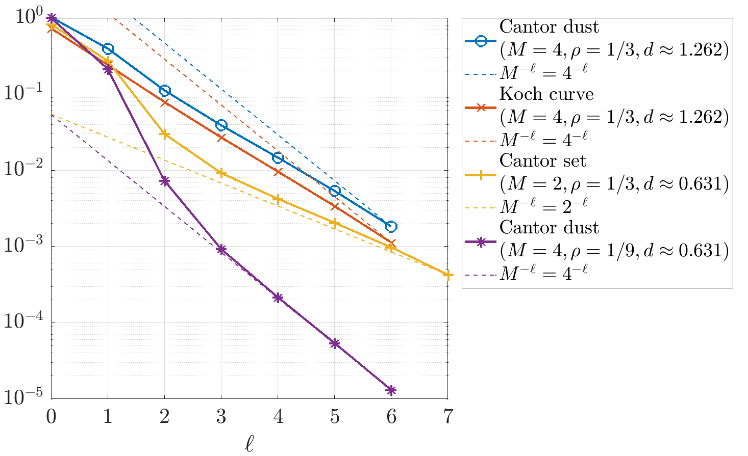
(b) Far-field relative $L^{\infty}$ errors

Figure 6: Plots of the discrete relative-error estimates (67) for a range of 2D examples.

5.1.2 Convergence plots

In Figure 6 we show the discrete $L^{\infty}$ relative errors (67) for a range of 2D examples, namely the Koch curve (Ex. 2.3), the Cantor set $C\times\{0\}$ (Ex. 2.2), and the Cantor dust $C\times C$ with two different values of $\rho$, with plane wave incidence direction $\vartheta=(1,-1)/\sqrt{2}$ and wavenumber $k=5$. To compute the scattered-field relative error given by (67) we sample at $50$ points equispaced along each edge of the square $(-1,2)\times(-1.5,1.5)$ (200 points in total), and for the far-field we sample at $50$ equispaced points on the circle $\mathbb{S}^{1}$. We use, for each scatterer, $\ell_{\mathrm{ref}}=\ell_{\max}+2$, where $\ell_{\max}$ is the largest $\ell$ for which results are shown.

Also plotted in Figure 6 are graphs of $cM^{-\ell}$, with $c>0$ chosen to fit each error curve. In the cases where Theorem 4.2 applies (all except the Koch curve), and, if Proposition 3.12 holds with $\epsilon=t_{d^{\prime}}$ (see the discussion in Remark 3.13), we expect, by Remark 4.3, errors to be roughly proportional to $M^{-\ell}$. In the examples with $d\approx 0.631$ the relative errors do seem to be proportional to $M^{-\ell}$ for larger $\ell$, supporting a conjecture that $\epsilon=t_{d^{\prime}}$ in these cases. The errors in the two examples with $d\approx 1.262$ seem to decrease at the same rate, suggesting the same solution regularity and that the error estimate of Theorem 4.2 holds also for the Koch curve case where $\Gamma$ is not disjoint. But the convergence is slower than $M^{-\ell}$, suggesting that the conjecture $\epsilon=t_{d^{\prime}}$, and the solution regularity it implies, do not hold in these cases.

5.1.3 The Koch snowflake

In Figure 7 we show approximations to ${\rm Re}(u^{t})$ for scattering by a Koch snowflake for the same incident plane wave as Figure 5, computed in two different ways, illustrating Remark 3.7. In Figure 7(a) we solve the IE by our Galerkin IEM with $N=4039$ on the solid Koch snowflake $\Gamma$, shown in Fig. 1(g), which is the attractor of an inhomogeneous IFS with $M=7$ as noted in Ex. 2.4. We refer to this as the volume approach. In Figure 7(b) we solve the IE by our Galerkin IEM on $\partial\Gamma$, the boundary of the snowflake. We refer to this as the boundary approach. In contrast to all our other examples, $\partial\Gamma$ is not an IFS attractor, but it is the union of three IFS attractors (rotated copies of the Koch curve of Ex. 2.3, each the attractor of an IFS with $M=4$), and so $\partial\Gamma$ is a $d$-set, with $d=d^{\prime}:={\rm dim_{H}}(\partial\Gamma)=\log(4)/\log(3)\approx 1.262$. In Figure 7(b) we use $M^{4}=256$ degrees of freedom on each Koch curve comprising $\partial\Gamma$, so that $N=768$.

In the boundary approach, to assemble the Galerkin matrix $\underline{\underline{A}}$, we view it as a $3\times 3$ block matrix, each block corresponding to interactions between two of the three Koch curves. The diagonal blocks correspond to self-interactions for a single Koch curve, and these matrix elements are approximated by quadrature as described at the beginning of the section. The off-diagonal blocks are assembled using the composite barycentre rule using the same value of $h_{Q}$ as for the diagonal blocks.

Proposition 3.6 and Remark 3.2 tell us that the IE solution in the volume approach is supported on $\partial\Gamma$, and that the IE solutions and scattered fields for the two approaches coincide as long as $k^{2}$ is not a Dirichlet eigenvalue of $-\Delta$ in $\Omega_{-}:=\Gamma^{\circ}$, the interior of the snowflake. It appears that $k=20$ is not one of these resonant wavenumbers as the fields in Figure 7(a) and (b) coincide and the field in $\Omega_{-}$ is zero in (b), in agreement with the boundary condition for the volume approach that $u^{t}\in\widetilde{H}{}^{1}(\Omega)$, where $\Omega=\Gamma^{c}$.

In Figure 8 we plot the modulus of the piecewise-constant Galerkin IEM solution $\phi_{N}\in V_{N}=Y_{h}\subset H_{\Gamma}^{-1}$ corresponding to Figure 7(a), for $h\approx 0.22$, $h\approx 0.074$, and $h\approx 0.025$. Since $\phi_{N}$ is constant on each element, the meshes used for each $h$ are discernible in Figure 8 (each element is a scaled copy of the original snowflake $\Gamma$). Each solution $\phi_{N}$ is highly peaked near $\partial\Gamma$, especially where $\partial\Gamma$ is illuminated by the incident wave, and is much smaller away from $\partial\Gamma$; these effects are increasingly marked as $h$ is reduced. This is unsurprising as, by Theorem 4.1, $\phi_{N}\to\phi$ in $H_{\Gamma}^{-1}$ as $h\to 0$, and $\phi$ is supported in $\partial\Gamma$. This implies that $\chi\phi_{N}\to\chi\phi=0$ in $H_{\Gamma}^{-1}$ as $h\to 0$ for every $\chi\in C_{0}^{\infty}(\Omega_{-})$, but it need not be the case that $\chi\phi_{N}\to 0$ in $L^{2}(\Omega_{-})$.

In Figure 7(c) we explore this convergence for the case where $\chi\in C_{0}^{\infty}(\Omega_{-})$ is given by $\chi(x):=\exp(-0.5/(0.2^{2}-|x|^{2}))$, for $|x|<0.2$, $\chi(x):=0$, for $|x|\geq 0.2$, showing computations for $h=\operatorname{diam}(\Gamma)/3^{\ell/2}$, for $\ell=0,1,\ldots,9$, which suggest that $\|\chi\phi_{N}\|_{L^{2}(\Omega_{-})}$ is bounded away from zero as $h\to 0$. On the other hand, since $\phi_{N}\to\phi$ in $H_{\Gamma}^{-1}$ and $\phi\in H_{\partial\Gamma}^{-1}$, $J(\phi_{N}):=(\varphi,\phi_{N})_{L^{2}(\Omega_{-})}=\langle\varphi,\phi_{N}\rangle_{H^{1}(\mathbb{R}^{2})\times H^{-1}(\mathbb{R}^{2})}\to 0$ as $h\to 0$ for all $\varphi\in C_{0}^{\infty}(\Omega_{-})$. In Figure 7(c) we also plot $|J(\phi_{N})|=|\int_{\Gamma}\varphi\overline{\phi_{N}}\mathrm{d}\mathcal{H}^{2}|$ against $\ell$ for a (rather arbitrary) selection of linearly independent $\varphi$, namely $\varphi=\chi^{2}$ and $\varphi=\chi_{\beta}$, for $\beta=0,\pi/4,\pi/2,3\pi/4$, where $\chi_{\beta}(x):=\chi^{2}(x)\exp({\mathrm{i}}kx\cdot\theta)$, $x\in\Omega_{-}$, with $\theta:=(\cos(\beta),\sin(\beta))$. For each of these choices, once $\ell\geq 4$, $|J(\phi_{N})|\to 0$ as $h\to 0$, at a faster rate than the $h^{d^{\prime}}$ rate of convergence that is predicted for linear functionals if Proposition 3.12 holds with $\epsilon=t_{d^{\prime}}$, by arguing as in Remark 4.3.

In Figure 7(d) we explore convergence of the far-field approximations $u_{\ell}^{\infty}$ computed by the volume and boundary approaches, showing computations for $h=\operatorname{diam}(\Gamma)/3^{\ell/2}$ for $\ell=0,1,\ldots,6$ for the volume approach, and $h=3\operatorname{diam}(\Gamma)/3^{\ell}$ for $\ell=0,1,\ldots,4$ for the boundary approach. For each approach we use as our “exact” solution the boundary approach solution with $\ell=\ell_{\mathrm{ref}}=7$. Figure 7(d) shows the relative errors (67) in $u_{\ell}^{\infty}$ for both methods, for plane wave incidence direction $\vartheta=(1,-1)/\sqrt{2}$ and $k=5$, with the $L^{\infty}$ norms computed using the same discrete set of points as in Figure 6. In the volume approach every second increment in $\ell$ has a smaller reduction in error. At these increments, the elements adjacent to $\partial\Gamma$, which is the support of the solution, are not being subdivided, as a consequence of the definition of the approximation space $Y_{h}$. The convergence rate results of Theorem 4.2 apply to the volume approach but not to the boundary approach as $\partial\Gamma$ is not an IFS attractor. But, assuming these estimates apply in both cases, and if Proposition 3.12 holds with $\epsilon=t_{d^{\prime}}$ so that the solution $\phi\in H_{\partial\Gamma}^{-1}$ has its maximum possible regularity, then, arguing as in Remark 4.3, we anticipate errors decreasing roughly in proportion to $h^{d^{\prime}}$ in both cases, i.e. proportional to $N^{-1}$ and $N^{-d^{\prime}/2}\approx N^{-0.631}$ in the respective boundary and volume cases. Both approaches appear to be converging somewhat more slowly than these conjectured theoretical rates, but the boundary approach is certainly converging more rapidly. It is plausible that the boundary approach, in which only $\partial\Gamma$ is discretised, should be more efficient, given that the solution is supported on $\partial\Gamma$. But the IE on $\partial\Gamma$ is not well-posed for all $k>0$ in contrast to the IE on $\Gamma$, and there must be scope to improve the efficiency of the volume approach by using graded versions of our meshes, concentrating elements near $\partial\Gamma$ (cf. [22]).

(a) ${\rm Re}(u^{t})$ for volume approach

(b) ${\rm Re}(u^{t})$ for boundary approach

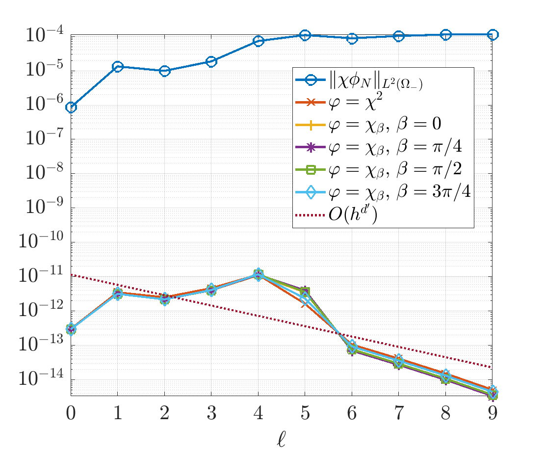
(c) $\|\chi\phi_{N}\|_{L^{2}(\Omega_{-})}$ and $|(\varphi,\phi_{N})_{L^{2}(\Omega_{-}}|$ for various $\varphi$

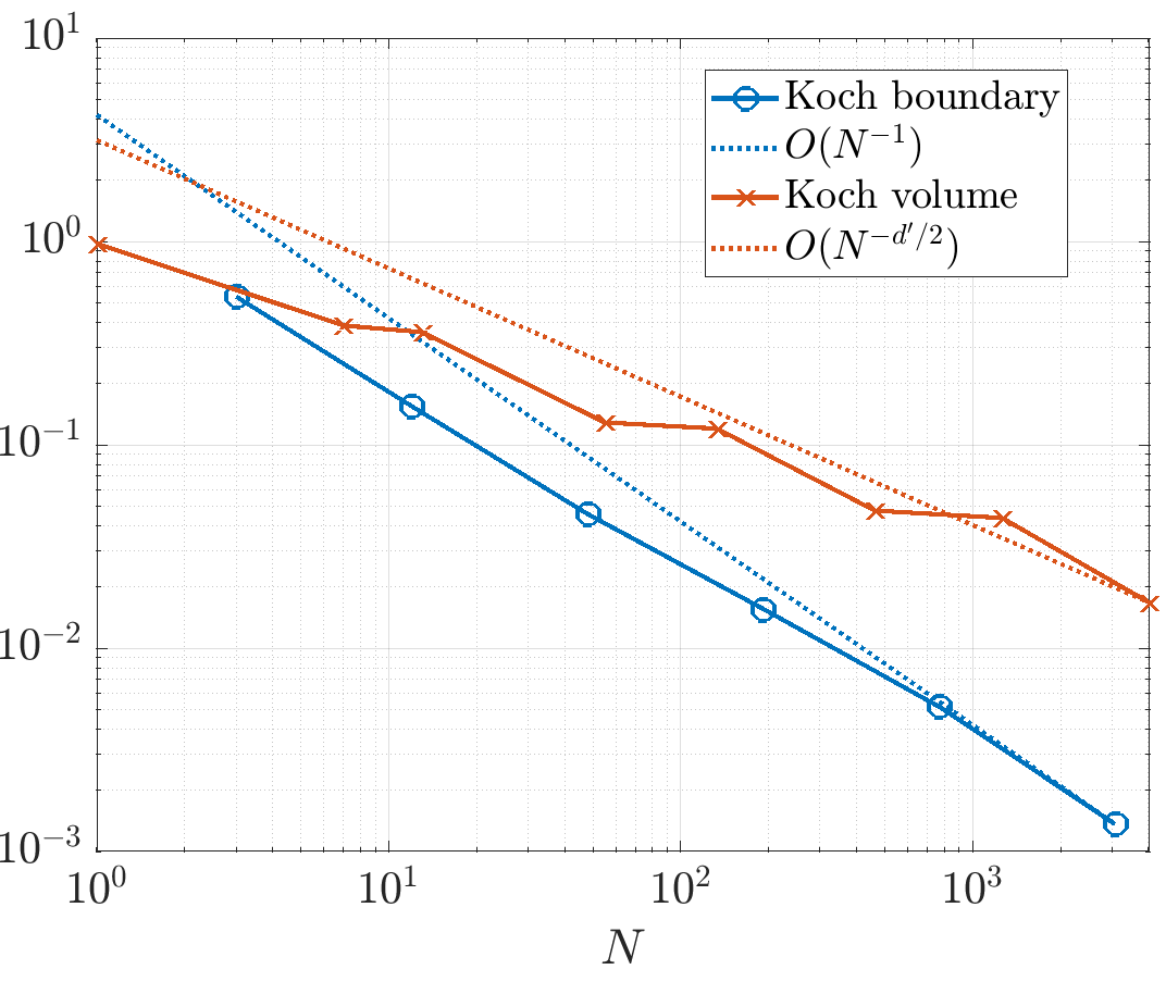
(d) Far-field relative $L^{\infty}$ errors

Figure 7: Scattering by the Koch snowflake. (a) and (b) show ${\rm Re}(u^{t})$ for $k=20$ computed with both approaches. For the same $k$, (c) plots $\|\chi\phi_{N}\|_{L^{2}(\Omega_{-})}$ and $|(\varphi,\phi_{N})_{L^{2}(\Omega_{-})}|$ for several $\varphi\in C_{0}^{\infty}(\Omega_{-})$, namely $\varphi=\chi^{2}$ and $\varphi=\chi_{\beta}$ for various $\beta$. (d) plots the far-field relative $L^{\infty}$ error for both approaches, for $k=5$.

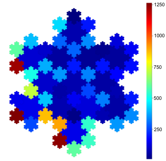
(a) $h=0.22$

(b) $h=0.074$

(c) $h=0.025$

Figure 8: $|\phi_{N}|$, where $\phi_{N}$ is the Galerkin IEM solution on the Koch snowflake, for a range of $h$.

5.2 Examples in 3D space

(a) $\rho=1/2$ and $d=2$

(b) $\rho=3/8$ and $d=\log(4)/\log(8/3)\approx 1.413$

Figure 9: ${\rm Re}(u_{\ell})$ for scattering by the Sierpinski tetrahedra of Figure 2 with $k=50$ and $\ell=7$.

In Figure 9 we show the real parts of the scattered fields created by the two Sierpinski tetradehra of Figure 2, which are attractors of the homogeneous IFS of Example 2.5 with $M=4$ and $d=\log 4/\log(1/\rho)$. The plane wave incidence direction is $\vartheta=(0,1,-1)/\sqrt{2}$, $k=50$, and both approximations were computed with $\ell=7$, corresponding to $N=16384$.

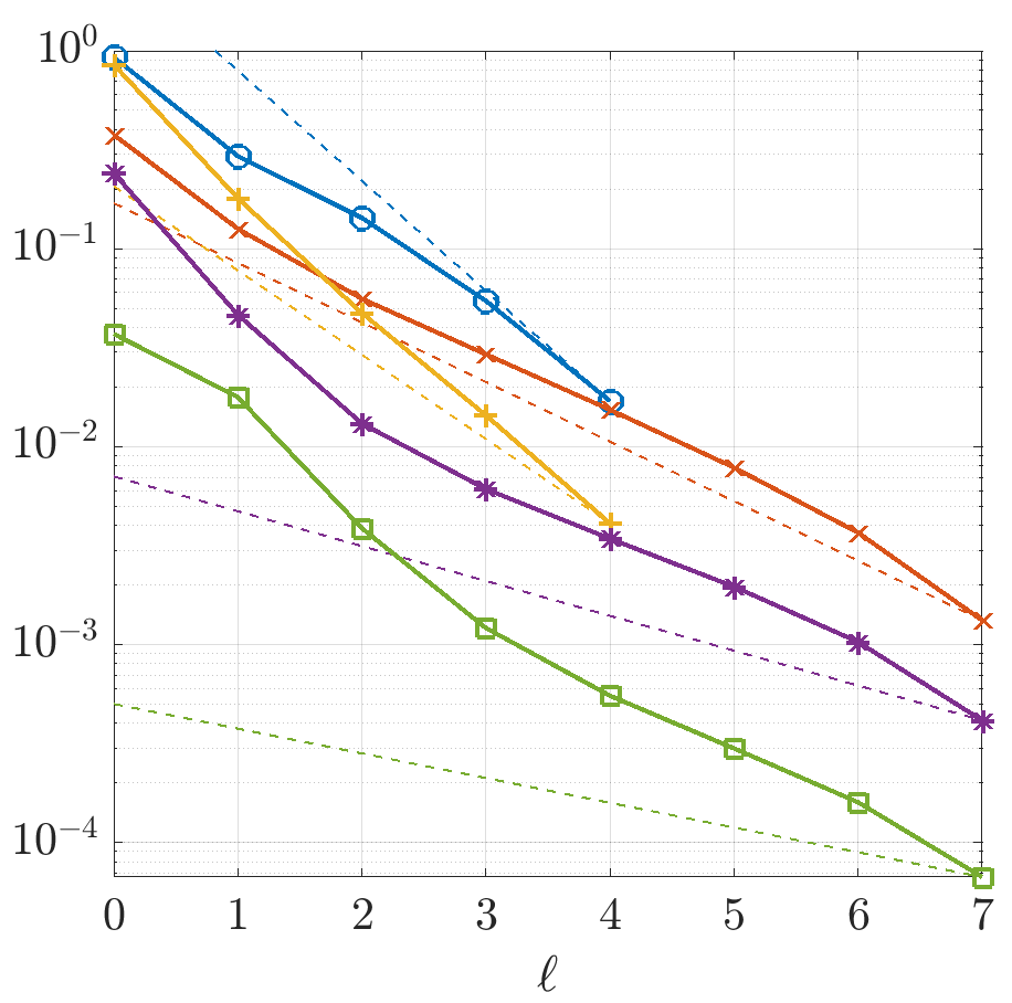
(a) Far-field relative $L^{\infty}$ errors

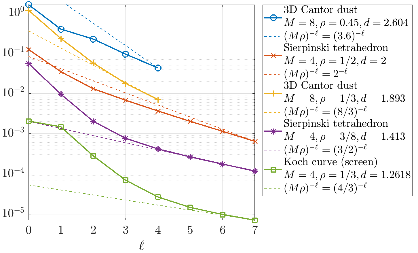
(b) Far-field $L^{\infty}$ absolute increment errors

Figure 10: $L^{\infty}$ convergence plots for a range of 3D examples.

In Figure 10 we show $L^{\infty}$ far-field errors for the same incidence direction and $k=2$ for a range of 3D examples, namely: the Sierpinski tetrahedra of Figures 2 and 9 and Example 2.5; 3D Cantor Dusts, i.e., $C\times C\times C$ where $C$ is the Cantor set of Example 2.2, with $\rho=1/3$ and $\rho=0.45$; the Koch curve of Figure 3 embedded in 3D space, i.e. $K\times\{0\}$, where $K\subset\mathbb{R}^{2}$ is the Koch curve of Example 2.3. All these scatterers $\Gamma$ have $d={\rm dim_{H}}(\Gamma)>1$ (see Figure 10) so that $H_{\Gamma}^{-1}$ is non-trivial by Remark 3.5, the Galerkin IEM is applicable, and the solution $\phi\in H_{\Gamma}^{-1}$ to the IE (32) is non-zero (since (32) is equivalent to (41) and $\mathrm{tr}_{\Gamma}g=-u^{i}|_{\Gamma}$ is non-zero), so also (by (26)) the scattered field $u=\mathcal{A}\phi$ is non-zero.

To compute the discrete $L^{\infty}$ relative errors (67) shown in Figure 10(a) we sample at $200$ points on the sphere $\mathbb{S}^{2}$, chosen so that the points form a uniform grid in spherical coordinate space $[0,\pi]\times[0,2\pi]$, and we use, for each scatterer, $\ell_{\mathrm{ref}}=\ell_{\max}+1$, where $\ell_{\max}$ is the largest $\ell$ for which results are shown. This choice of $\ell_{\mathrm{ref}}$, constrained by computational resources, is not large enough for $u^{\infty}_{\ell_{\mathrm{ref}}}$ to be a sufficiently accurate “exact” solution to see convergence rates clearly. Thus we also plot in Figure 10(b) the absolute increment errors $\|u^{\infty}_{\ell}-u^{\infty}_{\ell+1}\|_{L^{\infty}}$ for $\ell=0,\ldots,\ell_{\mathrm{ref}}-1$. As discussed in [5, §6.2], if, for some $c>0$ and $0<\alpha<1$, $\|u^{\infty}_{\ell}-u^{\infty}_{\ell+1}\|_{L^{\infty}}=c\alpha^{\ell}$ for all $\ell\geq\ell_{0}$ then, by the triangle rule, $\|u^{\infty}-u^{\infty}_{\ell}\|_{L^{\infty}}\leq\frac{c}{1-\alpha}\,\alpha^{\ell}$ for $\ell\geq\ell_{0}$. Thus convergence rates can be deduced from Figure 10(b). By Remark 4.3, which applies to all the examples except the Koch curve, we expect, provided Proposition 3.12 holds with $\epsilon=t_{d^{\prime}}$, to see errors roughly proportional to $(M\rho)^{-\ell}$. This convergence rate is observed in Figure 10(b) for sufficiently large $\ell$ for all the cases with $d<2$, but the convergence is significantly slower than $(M\rho)^{-\ell}$ for the example with $d\approx 2.6$. These results, and the convergence results reported in §5.1, suggest that a conjecture that $\epsilon=t_{d^{\prime}}$ in Proposition 3.12 does not hold in cases where $d^{\prime}={\rm dim_{H}}(\partial\Gamma)>n-1$ (note $\partial\Gamma=\Gamma$ for the scatterers in Figures 6 and 10), but does hold in cases where $d^{\prime}<n-1$. They suggest moreoever that this conjecture and the estimates of Theorem 4.2 hold for the non-disjoint 3D Koch curve case.

Appendix A Singular quadrature on fractals

In this appendix we briefly outline the methodology of [17, 16] for the derivation of representation formulas for singular integrals on fractals in terms of regular integrals. We assume throughout that $\Gamma$ is the attractor of an IFS satisfying the OSC.

The basic singular integral we consider is

$$I_{\Gamma,\Gamma}:=\int_{\Gamma}\int_{\Gamma}\widetilde{\Phi}_{t}(|x-y|)\,\mathrm{d}\mathcal{H}^{d}(x)\mathrm{d}\mathcal{H}^{d}(y),$$

where

$$\tilde{\Phi}_{t}(r):=\begin{cases}r^{-t},&t>0,\\ \log{r},&t=0.\end{cases}$$

The cases $t=0$ and $t=1$ are those relevant to §4(b), since $\Phi_{\rm sing}(x,y)=-\tilde{\Phi}_{0}(|x-y|)/(2\pi)$ for $n=2$, and $\Phi_{\rm sing}(x,y)=\tilde{\Phi}_{1}(|x-y|)/(4\pi)$ for $n=3$, but for completeness we consider the general case. The integral $I_{\Gamma,\Gamma}$ is finite if and only if $t<d$, where $d$ is the Haudsorff dimension of $\Gamma$ (see, e.g., [17, Cor. A.2] or [5, Cor. 2.3]), so we assume henceforth that $0\leq t<d$.

A.1 Similarity

The representation formulas and quadrature rules presented in [17, 16] are based on decomposing $I_{\Gamma,\Gamma}$ as a sum of integrals over self-similar subsets of $\Gamma$. For ${\boldsymbol{m}},{\boldsymbol{m}^{\prime}}\in\bigcup_{\ell=0}^{\infty}I_{\ell}$ we define

$$I_{{\boldsymbol{m}},{\boldsymbol{m}^{\prime}}}:=\int_{\Gamma_{\boldsymbol{m}}}\int_{\Gamma_{\boldsymbol{m}^{\prime}}}\widetilde{\Phi}_{t}(|x-y|)\,\mathrm{d}\mathcal{H}^{d}(x)\mathrm{d}\mathcal{H}^{d}(y),$$

which is singular when $\Gamma_{\boldsymbol{m}}\cap\Gamma_{\boldsymbol{m}^{\prime}}$ is non-empty, and regular otherwise. Key to the methodology of [17, 16] is that many of these integrals $I_{{\boldsymbol{m}},{\boldsymbol{m}^{\prime}}}$, for different choices of ${\boldsymbol{m}},{\boldsymbol{m}^{\prime}}$, can be related to each other using the self-similarity of $\Gamma$ and the homogeneity of $\tilde{\Phi}_{t}$, namely that, for $\rho>0$,

$$\tilde{\Phi}_{t}(\rho r)=\begin{cases}\rho^{-t}\tilde{\Phi}_{t}(r),&t>0,\\ \log\rho+\tilde{\Phi}_{t}(r),&t=0.\end{cases}$$ (68)

The following result is a consequence of [16, Props 3.2 & 3.3, Rem. 2.1]. Here $|{\boldsymbol{m}}|$ denotes the length of the vector index ${\boldsymbol{m}}$, with $|0|$ interpreted as $0$ in the case $\Gamma_{{\boldsymbol{m}}}=\Gamma_{0}=\Gamma$, and we define $\vartheta_{t}$ by $\vartheta_{t}:=0$ for $t>0$ and $\vartheta_{t}:=\mathcal{H}^{d}(\Gamma)^{2}$ for $t=0$. Adopting the terminology of [16], when the conditions of Proposition A.1 hold we say that the integrals $I_{{\boldsymbol{m}},{\boldsymbol{m}}^{\prime}}$ and $I_{{\boldsymbol{n}},{\boldsymbol{n}}^{\prime}}$ are similar. The condition (69) stipulates that there exist similarities mapping $\Gamma_{\boldsymbol{m}}$ to $\Gamma_{\boldsymbol{n}}$, and $\Gamma_{\boldsymbol{m}^{\prime}}$ to $\Gamma_{\boldsymbol{n}^{\prime}}$, defined in terms of the IFS and symmetry properties of $\Gamma$, that are compatible in a certain sense. We note that one can always take the isometries $T$ and $T^{\prime}$ to be the identity map in the following.

Proposition A.1.

Let ${\boldsymbol{m}},{\boldsymbol{m}^{\prime}},{\boldsymbol{n}},{\boldsymbol{n}^{\prime}}\in\bigcup_{\ell=0}^{\infty}I_{\ell}$. Let $T$ and $T^{\prime}$ be isometries of $\mathbb{R}^{n}$ such that $T(\Gamma)=T^{\prime}(\Gamma)=\Gamma$. Suppose there exists $\varrho>0$ such that

$$|s_{{\boldsymbol{m}}}(T(s_{{\boldsymbol{n}}}^{-1}(x)))-s_{{\boldsymbol{m}^{\prime}}}(T^{\prime}(s_{{\boldsymbol{n}^{\prime}}}^{-1}(y)))|=\varrho|x-y|,\quad x,y\in\mathbb{R}^{n}.$$ (69)

Then

$$\varrho=\frac{\rho_{\boldsymbol{m}}}{\rho_{\boldsymbol{n}}}=\frac{\rho_{\boldsymbol{m}^{\prime}}}{\rho_{\boldsymbol{n}^{\prime}}}$$ (70)

and

$$I_{{\boldsymbol{m}},{\boldsymbol{m}}^{\prime}}=\varrho^{2d-t}I_{{\boldsymbol{n}},{\boldsymbol{n}}^{\prime}}+\vartheta_{t}(\rho_{\boldsymbol{m}}\rho_{\boldsymbol{m}^{\prime}})^{d}\log{\varrho},\qquad t\in[0,d).$$ (71)

Furthermore, if $\Gamma$ is homogeneous then $|{\boldsymbol{m}}|-|{\boldsymbol{n}}|=|{\boldsymbol{m}^{\prime}}|-|{\boldsymbol{n}^{\prime}}|$, $\varrho=\rho^{|{\boldsymbol{m}}|-|{\boldsymbol{n}}|}$, and, noting that $\rho^{d}=1/M$, (71) can be written as

$$I_{{\boldsymbol{m}},{\boldsymbol{m}}^{\prime}}={\frac{\rho^{-t(|{\boldsymbol{m}}|-|{\boldsymbol{n}}|)}}{M^{2(|{\boldsymbol{m}}|-|{\boldsymbol{n}}|)}}I_{{\boldsymbol{n}},{\boldsymbol{n}}^{\prime}}+\vartheta_{t}\frac{(|{\boldsymbol{m}}|-|{\boldsymbol{n}}|)}{M^{|{\boldsymbol{m}}|+|{\boldsymbol{m}^{\prime}}|}}\log{\rho},}\qquad t\in[0,d).$$ (72)

The methodology of [17, 16] involves attempting to

• identify a finite number $n_{s}$ of “fundamental” singular integrals
  $I_{{\boldsymbol{m}}_{s,1},{\boldsymbol{m}^{\prime}}_{s,1}},\ldots,I_{{\boldsymbol{m}}_{s,n_{s}},{\boldsymbol{m}^{\prime}}_{s,n_{s}}}$, with $I_{{\boldsymbol{m}}_{s,1},{\boldsymbol{m}^{\prime}}_{s,1}}=I_{\Gamma,\Gamma}$, such that any other singular integral $I_{{\boldsymbol{m}},{\boldsymbol{m}^{\prime}}}$, for ${\boldsymbol{m}},{\boldsymbol{m}^{\prime}}\in L_{h}$, is similar to one of them in the sense of Proposition A.1 (via suitable $T,T^{\prime}$);

• derive an $n_{s}$-by-$n_{s}$ linear system of equations satisfied by these fundamental singular integrals, that can be solved to express them (and hence any similar singular integral) in terms of regular integrals that can be computed numerically (e.g. using the composite barycentre rule).

An algorithm for attempting to achieve (i) and (ii) in the general case is presented in [16, Algorithm 1], and the earlier results in [17, §4.3] can be viewed as a specialisation of this algorithm to the case of a disjoint attractor, for which $n_{s}=1$. The basic idea is to start from $I_{\Gamma,\Gamma}$ and combine repeated subdivision of the integration domain with repeated applications of Proposition A.1 to determine when integrals are similar. Whether the algorithm succeeds in achieving (i) and (ii) depends on the example being studied, but in [16, §5] it was shown to succeed for a number of well-known examples of non-disjoint attractors including the Sierpinski triangle, Vicsek fractal, Sierpinski carpet and the Koch snowflake. Rather than repeating the full details of the algorithm here, we instead exemplify the procedure in the case of the Koch curve (see Fig. 1(f)), which was not studied in [16].

A.2 Example - Koch curve

The Koch curve (see Ex. 2.3, Fig. 1(f) and Fig. 3) $\Gamma\subset\mathbb{R}^{2}$ is the attractor of a homogeneous IFS with $M=4$ and $\rho=1/3$, so that $d=\log{4}/\log{3}$ and $\rho^{d}=1/4$. The only isometries of $\mathbb{R}^{2}$ under which $\Gamma$ is invariant are the identity, and reflection in the line $x=1/2$.

To make the notation more compact, given ${\boldsymbol{m}}=(m_{1},m_{2},\ldots,m_{\ell})$ and ${\boldsymbol{m}^{\prime}}=(m_{1}^{\prime},m_{2}^{\prime},\ldots,m_{\ell^{\prime}}^{\prime})$ we write $\Gamma_{\boldsymbol{m}}$, $\Gamma_{\boldsymbol{m}^{\prime}}$ and $I_{{\boldsymbol{m}},{\boldsymbol{m}^{\prime}}}$ as $\Gamma_{m_{1}m_{2}\ldots m_{\ell}}$, $\Gamma_{m_{1}^{\prime}m_{2}^{\prime}\ldots m_{\ell^{\prime}}^{\prime}}$ and $I_{m_{1}m_{2}\ldots m_{\ell},m_{1}^{\prime}m_{2}^{\prime}\ldots m_{\ell^{\prime}}^{\prime}}$, respectively. For example, we write $I_{(1,3),(2,4)}$ as $I_{13,24}$. This compact notation is unambiguous because $M<10$, which ensures that each entry in ${\boldsymbol{m}}$ and ${\boldsymbol{m}^{\prime}}$ is a single-digit integer.

Using Proposition A.1 (with $\varrho=1$ and appropriate choices of $T$ and $T^{\prime}$) one can check that $I_{1,1}=I_{2,2}=I_{3,3}=I_{4,4}$, $I_{1,2}=I_{3,4}$, $I_{1,3}=I_{2,4}$, and $I_{i,j}=I_{j,i}$ for all $i,j\in\{1,\ldots,4\}$. Hence a level 1 decomposition of $I_{\Gamma,\Gamma}$ (illustrated in Fig. 3(a)) gives

$$I_{\Gamma,\Gamma}=\sum_{i=1}^{4}\sum_{j=1}^{4}I_{i,j}=4I_{1,1}+4I_{1,2}+2I_{2,3}+R_{\Gamma,\Gamma},$$ (73)

where $R_{\Gamma,\Gamma}$ is a sum of regular integrals, given by

$$R_{\Gamma,\Gamma}:=4I_{1,3}+2I_{1,4}.$$

The integral $I_{1,1}$ is singular, but by Proposition A.1 is similar to $I_{\Gamma,\Gamma}=I_{0,0}$, with

$$I_{1,1}=\frac{{3^{t}}}{16}I_{\Gamma,\Gamma}-\vartheta_{t}\frac{\log{3}}{16}.$$ (74)

The integrals $I_{1,2}$ and $I_{2,3}$ are also singular, since $\Gamma_{1}$ and $\Gamma_{2}$ intersect at a point, as do $\Gamma_{2}$ and $\Gamma_{3}$. But they are not similar to $I_{\Gamma,\Gamma}$, so we apply a level 2 decomposition (see Fig. 3(b)), writing

$$I_{1,2}=I_{14,21}+R_{1,2}\qquad\text{and}\qquad I_{2,3}=I_{24,31}+R_{2,3},$$ (75)

where $R_{1,2}$ and $R_{2,3}$ are both sums of regular integrals, given by

$$R_{1,2}=2I_{11,21}+2I_{11,22}+2I_{11,23}+I_{11,24}+2I_{12,21}+2I_{12,22}+I_{12,23}+2I_{13,21}+I_{13,22},$$

$$R_{2,3}=4I_{21,31}+2I_{21,32}+2I_{21,33}+2I_{21,34}+2I_{22,31}+2I_{23,31}+I_{23,32}.$$

The integrals $I_{14,21}$ and $I_{24,31}$ are both singular, but are similar to $I_{1,2}$ and $I_{2,3}$, with

$$I_{14,21}=\frac{{3^{t}}}{16}I_{1,2}-\vartheta_{t}\frac{\log{3}}{{256}},\qquad\text{and}\qquad I_{24,31}=\frac{{3^{t}}}{16}I_{2,3}-\vartheta_{t}\frac{\log{3}}{{256}}.$$ (76)

Combining (73)-(76), we find that the vector of fundamental singular integrals $(I_{\Gamma,\Gamma},I_{1,2},I_{2,3})^{T}$ satisfies the linear system

$$\left(\begin{array}[]{ccc}\sigma_{1}&-4&-2\\ 0&\sigma_{2}&0\\ 0&0&\sigma_{2}\end{array}\right)\left(\begin{array}[]{c}I_{\Gamma,\Gamma}\\ I_{1,2}\\ I_{2,3}\end{array}\right)=\left(\begin{array}[]{c}R_{\Gamma,\Gamma}-\vartheta_{t}\frac{\log{3}}{4}\\ R_{1,2}-\vartheta_{t}\frac{\log{3}}{{256}}\\ R_{2,3}-\vartheta_{t}\frac{\log{3}}{{256}}\end{array}\right),\qquad t\in[0,d),$$ (86)

where

$$\sigma_{1}=1-\frac{3^{t}}{4},\quad\sigma_{2}=1-\frac{3^{t}}{16}.$$

Solving the system gives

$$I_{2,3}=\frac{1}{\sigma_{2}}\Big{(}R_{2,3}-\vartheta_{t}\frac{\log{3}}{{256}}\Big{)},\qquad I_{1,2}=\frac{1}{\sigma_{2}}\Big{(}R_{1,2}-\vartheta_{t}\frac{\log{3}}{{256}}\Big{)},$$ (87)

and

$$I_{\Gamma,\Gamma}=\frac{1}{\sigma_{1}}\left(R_{\Gamma,\Gamma}+\frac{2}{\sigma_{2}}\Big{(}2R_{1,2}+R_{2,3}\Big{)}-\vartheta_{t}\Big{(}{32}+\frac{3}{\sigma_{2}}\Big{)}\frac{\log{3}}{{128}}\right).$$ (88)

Having derived the representation formulas (87)-(88), one can obtain numerical approximations of $I_{\Gamma,\Gamma}$, $I_{1,2}$ and $I_{2,3}$ by combining these with numerical evaluations of $R_{\Gamma,\Gamma}$, $R_{1,2}$ and $R_{2,3}$, e.g. using the composite barycentre rule with some maximum mesh width $\tilde{h}>0$.

To apply these results in the assembly of the Galerkin matrix considered in §4(b), we note that since we are using the approximation space $V_{N}=Y_{h}$ on the mesh $L_{h}$ of $\Gamma$, any singular instance of (4.17) will be similar to one of $I_{\Gamma,\Gamma}$, $I_{1,2}$ and $I_{2,3}$, say $I_{i,j}$. To evaluate (4.17) we apply Proposition A.1 to obtain a formula for (4.17) in terms of $I_{i,j}$, which can be evaluated using the value for $I_{i,j}$ already computed (as discussed above). For instance, referring back to Fig. 3(b) with ${\boldsymbol{m}}=(1,1,3)$ and ${\boldsymbol{m}^{\prime}}=(1,1,4)$ the integral (4.17) is similar to $I_{1,2}$, with

$$I_{113,114}=\frac{{3^{2t}}}{{256}}I_{1,2}-\vartheta_{t}\frac{\log{3}}{2048}.$$

To ensure parity between the quadrature accuracies for such singular instances of (4.17), and the regular instances of (4.17), which were computed using the composite barycentre rule with maximum mesh width $h_{Q}$, we take $\tilde{h}=h_{Q}/h$.

Acknowledgements

SC-W was supported by EPSRC grant EP/V007866/1, and DH and AG by EPSRC grants EP/S01375X/1 and EP/V053868/1. AM was supported by the PRIN project “NA-FROM-PDEs” and by PNRR-M4C2-I1.4-NC-HPC-Spoke6. AC was supported by CIDMA (Center for Research and Development in Mathematics and Applications) and FCT (Foundation for Science and Technology) within project UIDB/04106/2020. AG, SC-W, DH and AM would like to thank the Isaac Newton Institute for Mathematical Sciences for support and hospitality during the programme “Mathematical Theory and Applications of Multiple Wave Scattering” when work was undertaken supported by EPSRC grant EP/R014604/1. The authors acknowledge the use of the UCL Myriad High Performance Computing Facility (Myriad@UCL), and associated support services, in the completion of this work.

References

- [1] M. Abramowitz and I. A. Stegun, Handbook of Mathematical Functions with Formulas, Graphs, and Mathematical Tables, Dover, 1964.
- [2] J. Bannister, A. Gibbs, and D. P. Hewett, Acoustic scattering by impedance screens/cracks with fractal boundary: well-posedness analysis and boundary element approximation, Math. Mod. Meth. Appl. Sci. (M3AS), 32 (2022), pp. 291–319.
- [3] A. Caetano, D. P. Hewett, and A. Moiola, Density results for Sobolev, Besov and Triebel-Lizorkin spaces on rough sets, J. Funct. Anal., 281 (2021), p. 109019.
- [4] A. M. Caetano, S. N. Chandler-Wilde, A. Gibbs, and D. P. Hewett, Properties of IFS attractors with non-empty interiors and associated function spaces and scattering problems, In preparation.
- [5] A. M. Caetano, S. N. Chandler-Wilde, A. Gibbs, D. P. Hewett, and A. Moiola, A Hausdorff-measure boundary element method for acoustic scattering by fractal screens, Under review, arxiv preprint 2212.06594, (2022).
- [6] S. N. Chandler-Wilde, I. G. Graham, S. Langdon, and E. A. Spence, Numerical-asymptotic boundary integral methods in high-frequency acoustic scattering, Acta Numer., 21 (2012), pp. 89–305.
- [7] S. N. Chandler-Wilde and D. P. Hewett, Well-posed PDE and integral equation formulations for scattering by fractal screens, SIAM J. Math. Anal., 50 (2018), pp. 677–717.
- [8] S. N. Chandler-Wilde, D. P. Hewett, and A. Moiola, Interpolation of Hilbert and Sobolev spaces: quantitative estimates and counterexamples, Mathematika, 61 (2015), pp. 414–443.
- [9] , Sobolev spaces on non-Lipschitz subsets of with application to boundary integral equations on fractal screens, Integr. Equat. Operat. Th., 87 (2017), pp. 179–224.
- [10] S. N. Chandler-Wilde, D. P. Hewett, A. Moiola, and J. Besson, Boundary element methods for acoustic scattering by fractal screens, Numer. Math., 147 (2021), pp. 785–837.
- [11] S. N. Chandler-Wilde and P. Monk, Wave-number-explicit bounds in time-harmonic scattering, SIAM J. Math. Anal., 39 (2008), pp. 1428–1455.
- [12] X. Claeys and R. Hiptmair, Integral equations on multi-screens, Integr. Equat. Oper. Th., 77 (2013), pp. 167–197.
- [13] L. C. Evans, Partial Differential Equations, AMS, 2010.
- [14] L. C. Evans and R. E. Gariepy, Measure Theory and Fine Properties of Functions, CRC Press, revised ed., 2015.
- [15] K. Falconer, Fractal Geometry: Mathematical Foundations and Applications, Wiley, 3rd ed., 2014.
- [16] A. Gibbs, D. P. Hewett, and B. Major, Numerical evaluation of singular integrals on non-disjoint self-similar fractal sets, Under review, arxiv preprint 2303.13141, (2023).
- [17] A. Gibbs, D. P. Hewett, and A. Moiola, Numerical evaluation of singular integrals on fractal sets, Numer. Alg., 92 (2023), pp. 2071–2124.
- [18] D. P. Hewett and A. Moiola, On the maximal Sobolev regularity of distributions supported by subsets of Euclidean space, Anal. Appl., 15 (2017), pp. 731–770.
- [19] P. Jones, J. Ma, and V. Rokhlin, A fast direct algorithm for the solution of the Laplace equation on regions with fractal boundaries, J. Comput. Phys., 113 (1994), pp. 35–51.
- [20] A. Jonsson, Wavelets on fractals and Besov spaces, J. Fourier Anal. Appl., 4 (1998), pp. 329–340.
- [21] A. Jonsson and H. Wallin, Function Spaces on Subsets of , Math. Rep., 2 (1984).
- [22] B. N. Khoromskij and J. M. Melenk, Boundary concentrated finite element methods, SIAM J. Numer. Anal., 41 (2003), pp. 1–36.
- [23] V. G. Maz’ya, Sobolev Spaces with Applications to Elliptic Partial Differential Equations, Springer, 2nd ed., 2011.
- [24] W. McLean, Strongly Elliptic Systems and Boundary Integral Equations, CUP, 2000.
- [25] M. Mitrea and M. Taylor, Boundary layer methods for Lipschitz domains in Riemannian manifolds, J. Funct. Anal., 163 (1999), pp. 181–251.
- [26] P. Panagiotopoulos and O. Panagouli, The FEM and BEM for fractal boundaries and interfaces. Applications to unilateral problems, Comput. Struct., 64 (1997), pp. 329–339.
- [27] L. Riddle, . classic iterated function systems. larryriddle.agnesscott.org/ifs/ifs.htm, downloaded 18 July 2023.
- [28] S. A. Sauter and C. Schwab, Boundary Element Methods, Springer, 2011.
- [29] H. A. Schenck, Improved integral formulation for acoustic radiation problems, J. Acoust. Soc. Am., 44 (1968), pp. 41–58.
- [30] I. J. Šneıberg, Spectral properties of linear operators in interpolation families of Banach spaces, Mat. Issled, 9 (1974), pp. 214–229.
- [31] H. Triebel, Fractals and Spectra, Birkhäuser, 1997.
- [32] H. Triebel, Function spaces and wavelets on domains, European Mathematical Society, 2008.
- [33] T. W. Wu and A. F. Seybert, A weighted residual formulation for the CHIEF method in acoustics, J. Acoust. Soc. Am., 90 (1991), pp. 1608–1614.