Investigation of the nonlinear flame response to dual-frequency disturbances

The two-way interaction between the unsteady flame heat release rate and acoustic waves can lead to combustion instability within combustors. To understand and quantify the flame response to oncoming acoustic waves, previous studies have typically considered the flame dynamic response to pure tone forcing and assumed a dynamically linear or weakly nonlinear response. In this study, the introduction of excitation with two distinct frequencies denoted $St_{1}$ and $St_{2}$ is considered, including the effect of excitation amplitude in order to gain more insight into the nature of flame nonlinearities and their link with combustion instabilities. The investigation considers laminar flames and combines a low-order asymptotic analysis (up to third order in normalised excitation amplitude) with numerical methods based on the model framework of the $G$-equation. The importance of the propagation speed of the disturbance and its variation with frequency on the nonlinear response of the flame is highlighted. The influence path of the disturbance at one of the forcing frequencies, say $St_{2}$, on the flame dynamic response at the other forcing frequency $St_{1}$ is studied in detail. In concrete terms, the perturbation at $St_{2}$ acts in conjunction with the perturbation at $St_{1}$ to induce third-order nonlinear interactions in the flame kinematics, significantly altering the behavior of the flame response at $St_{1}$ (smoothing out the spatial wrinkling of the flame and further attenuating the heat-releasing-rate response), as compared to the case where the flame is only subjected to the excitation at $St_{1}$. Particularly, when the normalised forcing amplitudes at the two frequencies are 0.2 and 0.3 respectively, the heat release rate response at the former frequency is attenuated by over 40 % compared to the single-frequency response. This provides important insights into how nonlinearity due to frequency interactions can act to reduce the flame response.

I Introduction

With the development of high-thrust rocket engines, lean combustion aero-engines and land-based gas turbines, combustion instability has proven to be a persistent problem which can cause serious damage [1]. Combustion instability, also known as thermoacoustic instability, arises due to the interaction between flame heat release rate (HRR) fluctuations, oncoming flow perturbations upstream of the flame, and acoustic oscillations in the combustion chamber [2, 3, 4, 5]. Its understanding and prediction require an understanding of how the flame HRR fluctuations respond to upstream velocity perturbations [6, 7], often characterised by the ratio of normalised HRR fluctuation to normalised velocity perturbation. At low perturbation levels, the flame typically responds linearly to flow perturbations and this relation is quantified using a flame transfer function (FTF) [8]. As the perturbation amplitudes increase, the flame response becomes nonlinear, and in the case of it being weakly nonlinear is often characterised by a flame describing function (FDF) [9].

The FDF can be characterised through experiments [10, 11] and numerical simulations [12]. A simpler alternative, which is able to quantitatively describe the FTF/FDF for laminar flames [6, 13] and weakly turbulent flames [14, 15, 16], derives the flame model from the $G$-equation proposed by Markstein [17] for tracking infinitely thin flame fronts. Based on linearisation of the $G$-equation for inclined flames, Schuller et al. [6] derived an analytical unified model which included the convective effects of flow modulation upstream of the flame to quantify the FTF of laminar premixed flames. The obtained analytical solution was in good agreement with the experimental results [18]. Lieuwen [19] developed a nonlinear framework for the $G$-equation to analyse the nonlinear dynamics of a premixed flame in response to harmonic velocity perturbations, and was able to predict the experimentally observed nonlinear behaviour of the flame [20]. A more comprehensive characterisation of the nonlinear flame response is possible by considering perturbations with double or even multiple harmonics. As well as offering a more complete understanding of the flame nonlinearity, such studies are also directly relevant to experiments [21, 22, 23] and numerical simulations [24, 25, 26] exhibiting dual or multiple frequency oscillations. Balachandran et al. [21] conducted experiments investigating the nonlinear response of premixed flames at two different frequencies. With the introduction of sub-harmonics or higher harmonics, the formation and shedding of vortices change significantly. They elaborated on the possibility of suppressing instabilities by introducing additional excitation at carefully chosen frequencies to the flame. Lamraoui et al. [22] experimentally investigated combustion instability in a turbulent vortex burner with two non-harmonically related unstable modes at 180 Hz and 280 Hz. The flame dynamics and corresponding combustion instabilities change significantly due to the presence of an additional disturbance. Haeringer et al. [24] proposed an extended FDF based on the experimental phenomena of Albayrak et al. [23] as an efficient way to include higher harmonics of the flame response.

Han et al. [27] numerically investigated the effect of two strong perturbations at 160 Hz and 320 Hz on the nonlinear response of a lean premixed flame. The introduction of a higher frequency disturbance significantly changed the HRR fluctuation; The level of flame response at the fundamental frequency was reduced by 70$\%$ compared to that for a single frequency perturbation. Nevertheless, the prevailing literature falls short of providing explicit elucidation regarding the influence of the secondary perturbation frequency on the flame response correlated with the fundamental perturbation frequency when the pair of frequencies remain unassociated. This is very common in practical situations [22]. As linear analysis shows a pattern with more than one positive growth rate, it is difficult to determine the presence and stability of steady-state oscillations. Moeck et al. [28] proposed conditions for the existence and stability of single- or multi-mode steady-state oscillations and applied this method to a thermoacoustic model with two linearly unstable modes. In addition, Orchini and Juniper [13] presented the computation of a non-static flame dual-input describing function (FDIDF) based on the $G$-equation model of a laminar conical flame. To perform harmonic balance analysis, they neglected the harmonic response at higher frequencies and assumed that the HRR response is dominated by components at the two input frequencies. It was able to predict the onset of the Neimark-Sacker bifurcation and determine the frequency of oscillations around the limit cycle. Whereas, they treated the flame module as a “black box” embedded in the thermoacoustic network, which neglected the specific formation mechanism of the flame nonlinear response under two input perturbations. This hinders the understanding of some of the characteristics of FDIDF and further limits its application in more practical cases.

As mentioned above, there is a deviation in the flame nonlinear response to a perturbation at frequency $St_{1}$ ($St$ is the Strauhl number, defined by the angular frequency multiplied by the spatial distance divided by the mean bulk velocity), when there is also a simultaneous excitation at a different frequency $St_{2}$, compared to when $St_{1}$ is the only excitation frequency. How the flame nonlinear response at $St_{1}$ is affected by the disturbance at $St_{2}$ will be investigated in this work. This will be performed for general cases in which the frequency, amplitude and phase of the perturbation at $St_{2}$ are independent of those at $St_{1}$. The spatial distribution of the flame kinematics, and the HRR response will be considered to quantify and account for the full nonlinearity induced by the dual frequency excitation. The nonlinear results for the flame response are derived by considering a low-order asymptotic analysis (up to third order in normalised excitation amplitude) applied to numerical computation of the flame based on the model framework of the $G$-equation. This is described in section II. The mechanisms by which the perturbation at $St_{2}$ affects the spatial kinematics of the flame at $St_{1}$ are discussed. These results are presented in section III. The role of the perturbation at $St_{2}$ in the flame global response at $St_{1}$ is quantified, and the corresponding mechanisms are carefully discussed in section IV.

II Formulation

This section presents analytical and numerical methods for determining the nonlinear acoustic response of laminar premixed conical and V-shaped flames to dual-input perturbations. Conical and V-shaped flames are anchored on the burner rim as shown in figure 1 (a) and (b) respectively, where the symmetrical flames are subjected to two velocity perturbations $u_{1}^{\prime}$ and $u_{2}^{\prime}$ with different frequencies. The dynamics of the flame front are quantified based on the $G$-equation model proposed by Markstein [17] for tracking thin laminar or weakly turbulent premixed flame fronts [8, 19], The instantaneous premixed flame front-tracking is given by

$$\frac{{\partial G}}{{\partial t}}+{\bm{u}}\cdot\nabla G={S_{L}}\left|{\nabla G}\right|$$ (1)

where, $\bm{u}$ and $S_{L}$ are respectively the local velocity vector and laminar flame displacement speed, and the latter accounts for the kinematics of flame front; $G$ denotes a smooth scaler field, where $G=0$ indicates the flame front separating the reactants ($G<0$) and products ($G>0$). Equation (1) assumes that: (i) An infinitely thin flame front separates the unburned and burned regions. (ii) The flame laminar displacement speed is constant, which assumes a spatial-temporally constant equivalence ratio and omits the flame curvature effect. (iii) The flow condition upstream of the flame front is pre-defined, and both heat diffusion and thermal expansion are neglected. This implies weak density change across the flame front. (iv) The flame front is assumed to be a single-valued function of spatial location.

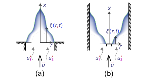
Figure 1: Sketches of (a) the conical flame and (b) the V-shaped flame subjected to dual-input disturbances ($x,r$ the spatial coordinate; $\xi\left(r,t\right)$ the flame front location; $t$ the time; $u_{1}^{\prime},u_{2}^{\prime}$ the perturbations at $St_{1}$ and $St_{2}$ and $\bar{u}$ the mean bulk velocity).

In a cylindrical coordinate system, equation (1) is rewritten under $x-r-\theta$ coordinates as,

$$\frac{{\partial G}}{{\partial t}}+u\frac{{\partial G}}{{\partial x}}+{u_{r}}\frac{{\partial G}}{{\partial r}}+\frac{{{u_{\theta}}}}{r}\frac{{\partial G}}{{\partial\theta}}={S_{L}}\sqrt{{{\left({\frac{{\partial G}}{{\partial x}}}\right)}^{2}}+{{\left({\frac{{\partial G}}{{\partial r}}}\right)}^{2}}+{{\left({\frac{1}{r}\frac{{\partial G}}{{\partial\theta}}}\right)}^{2}}}$$ (2)

where, $x$, $r$ and $\theta$ denote the spatial location; $t$ is the time; $u$, $u_{r}$ and $u_{\theta}$ are the velocity in the $x-$, $r-$ and $\theta-$directions respectively. According to assumption (iv), $G\left({x,r,\theta,t}\right)$ is transformed into explicit form with respect to the instantaneous flame front $\xi\left({r,\theta,t}\right)$ (it means that, for a given radial position, only one axial position of the flame front is possible at a given instant; Although this is not entirely consistent with experimental observations, which show large sharp angles and different axial positions of the flame front for a given radius, it captures the main features of nonlinear flame response to excitations in both laminar and turbulent cases [29, 30]):

$$G\left({x,r,\theta,t}\right)=x-\xi\left({r,\theta,t}\right)$$ (3)

Substituting equation (3) into equation (2), it can then be assumed that the parametric variation in the $\theta$-direction can be neglected (in this particular case, it has been justified and widely used in similar studies [19, 31]). In addition, the experimental results obtained by Birbaud et al. [32] indicate that velocity fluctuations are almost unchanged in the radial direction. The governing equation for the flame front location then simplifies to

$$\frac{{\partial\xi}}{{\partial t}}-u=-{S_{L}}\sqrt{1+{{\left({\frac{{\partial\xi}}{{\partial r}}}\right)}^{2}}}.$$ (4)

For the remainder of this paper, all parameters are normalised, i.e., velocities are normalised by the mean bulk velocity $\bar{u}$, spatial coordinates are normalised by the burner radius $\it\Omega$ and time by ${\it\Omega}/\bar{u}$. Since the flames are always anchored on the burner rim, boundary conditions of the governing equation (4) for different flames are given by

$${\xi_{\rm{C}}}\left({r=1,t}\right)=0;{\xi_{\rm{V}}}\left({r={\it\Omega_{b}},t}\right)=0$$ (5)

where subscripts “C” and “V” denote conical and V-shaped flames respectively; ${\it\Omega_{b}}$ is the radius of the centre body in the V-shaped flame case.

The velocity field upstream of the flame is presented in figure 1 and is expressed as the superposition of a mean flow and two disturbances:

$$u\left({S{t_{1}},S{t_{2}},x,t}\right)=1+{\epsilon_{1}}{{\cal C}_{1}}\left({S{t_{1}},x,t}\right)+{\epsilon_{2}}{{\cal C}_{2}}\left({S{t_{2}},x,t,\delta}\right)$$ (6)

herein, $\mathcal{C}$ is a source of acoustic disturbances and $\epsilon$ denotes perturbation amplitude; subscripts “1” and “2” denote the perturbations at $St_{1}$ and $St_{2}$ respectively. It should be noted that there is no essential difference between the two excitations other than a naming difference. The specific forms of the perturbation sources are given by

$$\left\{\begin{array}[]{l}{\mathcal{C}_{1}}\left({S{t_{1}},x,t}\right)=\cos\left[{S{t_{1}}\left({K_{1}x-t}\right)}\right]\\ {\mathcal{C}_{2}}\left({S{t_{2}},x,t,\delta}\right)=\cos\left[{S{t_{2}}\left({K_{2}x-t}\right)+\delta}\right]\end{array}\right.$$ (7)

where $St=\omega{\it\Omega}/\bar{u}$ is the normalised angular frequency, $\omega$ is angular frequency; $\delta$ is the phase difference of two perturbations; $K_{1}$ and $K_{2}$ characterise the perturbation convection speed $u_{c}$ and are expressed as $\bar{u}/u_{c}$. The perturbation propagates at the mean bulk velocity or speed of sound, corresponding to $K$ equals unity or tending to zero. Previous experimental studies [32, 33, 34] and numerical simulations [35] have highlighted that the propagation of disturbances changes significantly as the modulation frequency $St$ upstream of the flame changes. Recent work [36] has emphasized that the need to calibrate $u_{c}$ arises from neglecting thermal diffusion and thermal expansion in the $G$-equation model. The propagation of the disturbance along the flame sheet and the feedback to the velocity disturbances are responsible for $u_{c}$. Therefore, $K$ in the $G$-equation should be considered as an input parameter that requires calibration. However, in reality, the propagation velocities cannot be “input” because they are caused by flame flow feedback. one introduces a simplified derivation (referred to as the low-order modelling) that builds upon and expands the research conducted by Birbaud et al. [32]. The goal is to circumvent the aforementioned conflicts while encapsulating the key characteristics of the $St$ and $K$ relationship. Assuming the flow is incompressible and irrotational upstream of flame, the velocity potential $\psi$ satisfies the Laplace equation, whose form in cylindrical coordinates is,

$$\frac{{{\partial^{2}}\psi}}{{\partial{x^{2}}}}+\frac{1}{r}\frac{{\partial\psi}}{{\partial r}}+\frac{{{\partial^{2}}\psi}}{{\partial{r^{2}}}}=0.$$ (8)

Due to the presence of disturbances, $\psi$ is assumed to be in a wave-like form

$$\psi\sim g\left(r\right)\exp\left[{{\rm i}St\left({x-t}\right)}\right].$$ (9)

Substituting equation (9) into equation (8), the ordinary differential equation for the radial velocity potential distribution becomes

$$\frac{{{{\rm{d}}^{2}}g\left(r\right)}}{{{\rm{d}}{r^{2}}}}+\frac{1}{r}\frac{{{\rm{d}}g\left(r\right)}}{{{\rm{d}}r}}-St^{2}g\left(r\right)=0.$$ (10)

This has the general solution,

$$g\left(r\right)={A_{1}}{I_{0}}\left({Str}\right)+{A_{2}}{N_{0}}\left({Str}\right)$$ (11)

where $I_{0}$ and $N_{0}$ are the zero-order modified Bessel functions. The radial velocity component vanishes on the centreline $r=0$, resulting in $A_{2}=0$. The radial velocity component ${\left.{\partial\psi/\partial r}\right|_{r=R}}=B\cos\alpha\exp\left[{{\rm i}St\left({x-t}\right)}\right]$ on the flame front, where $B$ and $\alpha$ are a pre-exponential coefficient and the half angle of the flame tip respectively. Substituting the expression of $\psi$ into the boundary condition of flame front, one obtains $g\left(r\right)=B{I_{0}}\left({Str}\right)/{I_{1}}\left({StR}\right)$, corresponding to the velocity potential solution

$$\psi\left({St,r,x}\right)=\frac{{B{I_{0}}\left({Str}\right)}}{{{I_{1}}\left[{St\eta\left(x\right)}\right]}}\exp\left[{{\rm i}St\left({x-t}\right)}\right]$$ (12)

herein, $\eta\left(x\right)$ is flame front location, which is a function of $x$. Thus, the relative velocity potential $\vartheta$, defined as the ratio of the velocity potential on the reactant side to that on the flame front, is given by

$$\vartheta\left({St,r,x}\right)=\frac{{{I_{0}}\left({Str}\right)}}{{{I_{0}}\left[{St\eta\left(x\right)}\right]}}$$ (13)

If $\vartheta$ is smaller than a certain value (named the threshold $\Lambda$), the perturbation speed is assumed to be the speed of sound, i.e.,

$$\kappa\left({St,r,x}\right)=0~{}\rm{when}~{}\vartheta\left({St,r,x}\right)<\Lambda$$ (14)

where $\kappa=\bar{u}/u_{c}\left(r,x\right)$ is the spatial parameter at the unburned gas side. Conversely, when $\vartheta$ exceeds the threshold $\Lambda$, the perturbation is convected by the mean bulk velocity, i.e.,

$$\kappa\left({St,r,x}\right)=1~{}\rm{when}~{}\vartheta\left({St,r,x}\right)\geq\Lambda.$$ (15)

These features have been experimentally validated, where Birbaud et al. [32] assumed a threshold of $\Lambda=0.1$. The analytical results obtained show a good match to the experimental velocity perturbation measured upstream of the flame by particle image velocimetry (PIV). Recently, Yang et al. [34] conducted similar experiments and found that a threshold of $\Lambda=0.2$ reproduced the experimental results better. Based on the above derivation, one obtains the relation between $St$ and $\kappa$. Thus, the global $K$ representing the overall characteristics on the reactant side is quantified as

$$K\left({St}\right)=\int_{\theta=0}^{2\pi}{{\rm{d}}\theta\int_{x}{\int_{r}{\kappa\left({St,r,x}\right)r{\rm{d}}}x{\rm{d}}r}}/\int_{\theta=0}^{2\pi}{{\rm{d}}\theta\int_{x}{\int_{r}r{\rm{d}}x{\rm{d}}r}}$$ (16)

The connection between $K$ and $St$ differs for various flames due to the distinctions in steady flame front tracking and boundary condition expressions for conical and V-shaped flames. Figure 2 illustrates the relation between $St$ and $K$ for different threshold values and flame types. A generally consistent conclusion emerges: at low frequencies, the inflow disturbance is conveyed by the average bulk velocity, and this propagation speed of disturbance rises with the modulation frequency. When the forced frequency is large enough, $u_{c}$ approaches the speed of sound. At mid-frequencies, the perturbation propagation exhibits mixed characteristics, i.e., $u_{c}$ varies with position and does not have a uniform character, and the corresponding spatially averaged value $\bar{u_{c}}$ is localized in the range of $\bar{u}$ and $c$. This apparent three frequency-dependent behaviors are fully consistent in a qualitative sense with experiments [32] and numerical simulations [35]. Obviously, $\Lambda$ has a significant impact on the final relationship between $K$ and $St$. Here, we provide a potential explanation for the significant variation of the correlation between $St$ and $u_{c}$ with $\Lambda$: $\Lambda$ actually dominates the final result of the propagation of these perturbations, altering the $\kappa$ through the equations (14) and (15), in which it rises and $u_{c}$ tends more easily to the speed of sound. However, it should be remembered that $\Lambda$ is only an empirical value and needs to be correlated with experimental data. For the remainder of this study, $\Lambda=0.2$ is selected to align with the PIV results obtained by Yang et al. [34]. For various flame types, the V-shaped flame’s perturbation convection velocity is more prone to display uniform model ($K=0$) characteristics than the conical flame. In fact, the above analysis focuses on the case of a conical flame, ignoring the case of a V-shaped flame and the differences between the two flames. The V-shaped flame here is a simplified case of an inverted laminar flow conical flame that ignores the effect of eddy currents on flame kinematics. By presenting this V-shaped flame, the nonlinear effects of perturbations on the spatial and global response of the flame are easily emphasized, which will be focused on later. In addition, this method cannot capture $u_{c}$ smaller than $\bar{u}$ ($K>1$), which has been detailed in some experiments [32, 33] and numerical simulations [35] for specific spatial locations at particular frequencies. However, most analytical work on laminar premixed flames roughly assumes $K$ to be 0 or 1 and neglects the effect of modulation frequency on it. This approach is an enhancement, as $K$ is quantitatively determined by the influence of $St$ in the 0 to 1 range. As a result, employing this method to quantify $u_{c}$ is reasonable.

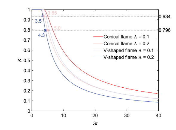
Figure 2: Dependence of $K$ on $St$ for different thresholds $\Lambda$ for different flames (${\it\Omega_{b}}=0$ for the V-shaped flame).

II.1 Numerical approach

In order to obtain fully nonlinear solutions of equation (4), the following numerical methods are used. The discretisations of spatial derivations use a seventh-order Weighted Essentially Non-Oscillatory (WENO7) scheme [37]. Since nodes only exist in the computational domain, the spatial derivatives at the boundary nodes are discretised using the fifth-order accurate upwind-differencing. A fifth-stage fourth-order Runge-Kutta method with Strong Stability Preserving (SSP-RK45) [38] is employed for time integration and the Local Lax-Friedrich (LLF) scheme [37] is used for improved stability. The grid size of a spatial discrete unit is $2\pi St/\left(200K\right)$ and the time step size is determined by the Courant-Friedrichs-Levy (CFL) number, i.e., $\textrm{CFL}=0.2$.

II.2 Low-order asymptotic analysis

An asymptotic analysis of the governing equation is used to gain insights into the key mechanisms underpinning the nonlinear interaction of the two perturbations. Asymptotic analysis is extended up to the third order of the excitation amplitudes $\epsilon_{1}$ and $\epsilon_{2}$, as follows,

$$\begin{split}\xi\left({r,t}\right)&=\underbrace{{\xi_{0}}\left(r\right)}_{{\rm{Steady\,term}}}+\underbrace{{\epsilon_{1}}{\xi_{1}}\left({r,t}\right)+{\epsilon_{2}}{\xi_{2}}\left({r,t}\right)}_{{\rm{Linear\,terms}}}\\ &+\underbrace{{\epsilon_{1}}^{2}{\xi_{1,1}}\left({r,t}\right)+{\epsilon_{2}}^{2}{\xi_{2,2}}\left({r,t}\right)+{\epsilon_{1}}^{3}{\xi_{1,1,1}}\left({r,t}\right)+{\epsilon_{2}}^{3}{\xi_{2,2,2}}\left({r,t}\right)}_{{\rm{Self-nonlinear\,terms}}}\\ &+\underbrace{{\epsilon_{1}}{\epsilon_{2}}{\xi_{1,2}}\left({r,t}\right)+{\epsilon_{1}}^{2}{\epsilon_{2}}{\xi_{1,1,2}}\left({r,t}\right)+{\epsilon_{1}}{\epsilon_{2}}^{2}{\xi_{1,2,2}}\left({r,t}\right)}_{{\rm{Mutual-nonlinear\,terms}}}\\ &+{O}\left[{{{\left({{\epsilon_{1}},{\epsilon_{2}}}\right)}^{4}}}\right]\end{split}$$ (17)

Herein, these ten terms are categorised into three types: linear terms, self-nonlinear terms and mutual nonlinear terms, which have corresponding physical meanings. Linear and self-nonlinear terms correspond to linear and nonlinear responses of the flame front-response, respectively, subjected purely to the perturbations at $St_{1}$ or $St_{2}$. Mutual-nonlinear terms account for the nonlinear kinematic response of the flame front location to two simultaneous perturbations. The steady-term solutions for different flames can be easily obtained, as follows,

$${\xi_{\rm{C},0}}\left(r\right)=\left({1-r}\right)\cot\alpha;{\xi_{\rm{V},0}}\left(r\right)=r\cot\alpha$$ (18)

where, $\alpha$ represents the half angle of the steady flame tip. Substituting equation (17) into the nonlinear source on the right-hand side (RHS) of equation (4), and extending the Taylor expansion to the third order, it can be expressed as

$$\sqrt{1+{{\left({\frac{{\partial\xi}}{{\partial r}}}\right)}^{2}}}\approx{\iota_{0}}{\rm{+}}{\iota_{1}}\left({\frac{{\partial\xi}}{{\partial r}}-\frac{{\partial{\xi_{0}}}}{{\partial r}}}\right)+\frac{1}{2}{\iota_{2}}{\left({\frac{{\partial\xi}}{{\partial r}}-\frac{{\partial{\xi_{0}}}}{{\partial r}}}\right)^{2}}$$ (19)

where,

$$\begin{split}&{\iota_{0}}={\left[{1+{{\left({\frac{{\partial{\xi_{0}}}}{{\partial r}}}\right)}^{2}}}\right]^{1/2}};\\ &{\iota_{1}}=\frac{{\partial{\xi_{0}}}}{{\partial r}}{\left[{1+{{\left({\frac{{\partial{\xi_{0}}}}{{\partial r}}}\right)}^{2}}}\right]^{-1/2}};\\ &{\iota_{2}}={\left[{1+{{\left({\frac{{\partial{\xi_{0}}}}{{\partial r}}}\right)}^{2}}}\right]^{-1/2}}-{\left({\frac{{\partial{\xi_{0}}}}{{\partial r}}}\right)^{2}}{\left[{1+{{\left({\frac{{\partial{\xi_{0}}}}{{\partial r}}}\right)}^{2}}}\right]^{-3/2}}.\end{split}$$ (20)

The nonlinear source has a specific physical meaning, in that it describes the flame propagating forward normal to itself.

According to the standard procedure of asymptotic analysis, the detailed solution of each corresponding term in equation (17) can be obtained. The specific forms of terms from asymptotic analysis are described in appendix VI (equations (40) $\sim$ (48)).

From the main issue to be discussed in this work, concise results were examined for each term, three of which (equations (40), (44) and (48)) were identified to be directly related to the flame kinematics at $St_{1}$. The specific expression is given by

$$\begin{split}{\xi_{S{t_{1}}}}\left({r,t}\right)&=\underbrace{{\epsilon_{1}}{\xi_{1}}\left({r,t}\right)}_{{\rm{Linear\,solution}}}+\underbrace{{\epsilon_{1}}^{3}{\xi_{{\rm{I}},{\rm{1}},{\rm{1}},{\rm{1}}}}\left({r,t}\right)}_{{\rm{Self-nonlinear\,solution}}}+\underbrace{{\epsilon_{1}}{\epsilon_{2}}^{2}{\xi_{{\rm{I}},{\rm{1}},{\rm{2}},{\rm{2}}}}\left({r,t}\right)}_{{\rm{Mutual-nonlinear\,solution}}}\\ &={\epsilon_{1}}{{\mu_{1}}\left(r\right)}\cos\left[{S{t_{1}}t+{\chi_{1}}\left(r\right)}\right]+{\epsilon_{1}}^{3}{{\mu_{{\rm{I}},1,1,1}}\left(r\right)}\cos\left[{S{t_{1}}t+{\chi_{{\rm{I}},1,1,1}}\left(r\right)}\right]+{\epsilon_{1}}{\epsilon_{2}}^{2}{{\mu_{{\rm{I}},{\rm{1}},{\rm{2}},{\rm{2}}}}\left(r\right)}\cos\left[{S{t_{1}}t+{\chi_{{\rm{I}},{\rm{1}},{\rm{2}},{\rm{2}}}}\left(r\right)}\right]\\ &={{\mu_{St_{1}}}\left(r\right)}\cos\left[{S{t_{1}}t+{\chi_{St_{1}}}\left(r\right)}\right]\end{split}$$ (21)

where the subscript “$St_{1}$” denotes the solution at $St_{1}$, $\mu\left(r\right)$ and $\chi\left(r\right)$ denote the magnitude and phase of the flame spatial response. These three components have their clear physical meaning; The first term describes the linear response of the flame kinematics to excitation at $St_{1}$; The nonlinearity of flame kinematic restoration is responsible for the remaining two terms. The formulation path of two third-order terms in equation (21) has been identified from the perspective of low-order asymptotic analysis. The former (named self-nonlinear term, $\xi_{\rm{I},1,1,1}$) is a result of perturbation at $St_{1}$, while the latter (named mutual-nonlinear term, $\xi_{\rm{I},1,2,2}$) is caused by excitations not only at $St_{1}$, but also at $St_{2}$. The term $\xi_{\rm{I},1,2,2}$ is significant, as it directly changes the flame response behaviour at $St_{1}$ due to perturbation at $St_{2}$. In other terms, $\xi_{\rm{I},1,2,2}$ accounts for the variation in flame kinematics at $St_{1}$ when an excitation at the frequency $St_{2}$ is applied. This demonstrates that asymptotic analysis serves as an efficient method for assessing the influence of linear, self-nonlinear, and mutually nonlinear responses arising from perturbations at $St_{2}$ and $St_{1}$ on flame kinematics at $St_{1}$, ultimately offering a better comprehension of their function in flame front-tracking.

III Flame spatial kinematics

In this section, the spatial kinematics of conical and V-shaped flames at $St_{1}$ under two-frequency excitations are analysed asymptotically. Numerical methods are also used to validate the accuracy of the analytical results, and the corresponding results are presented. One assumes that the response contains all the possible combinations of frequencies $St_{1}$ and $St_{2}$, and neglects the sub-harmonics of the input frequencies. The double Fourier series expansion [39] is used for the flame front expression, that is

$$\xi\left({r,t}\right)=\sum\limits_{m}{\sum\limits_{n}{{{\mu^{N}_{mSt_{1}+nSt_{2}}}\left(r\right)}}}\cos\left[{\left({mS{t_{1}}+nS{t_{2}}}\right)t{+}{\chi^{N}_{mSt_{1}+nSt_{2}}}\left(r\right)}\right]+\xi_{0}\left({r}\right)$$ (22)

where, $m,n\in\mathbb{Z}$, and the superscript “$N$” denotes the numerical result. As mentioned above, the main focus of this work is on results of flame kinematics at $St_{1}$, so only the numerical results at $St_{1}$ are extracted from equation (22).

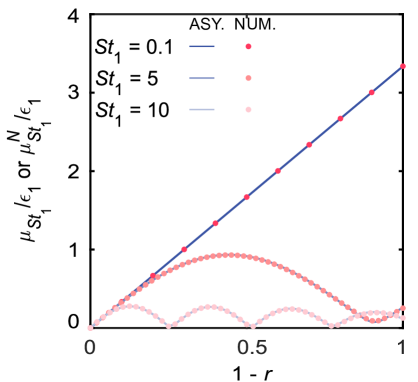
Figure 3: Validation of the spatial response at $St_{1}$ induced by asymptotic analysis in the conical flame. $\epsilon_{1}=0.2,\epsilon_{2}=0.1$ and $\delta=\pi/4$ in the case of $R=1.6$; Sold lines and markers denote the asymptotic and numerical results respectively. (The superscript “$N$” denotes numerical results, $R=St_{2}/St_{1}$, $\cot\alpha=3$.)

Figure 3 compares the relative magnitude of the numerical and asymptotic solutions in the response of the flame front-tracking at $St_{1}$ under two excitations. The spatial response amplitudes of the flame at $St_{1}$ obtained by asymptotic analysis are in good agreement with those determined by the numerical method in the face of different cases of perturbation inputs. This means that asymptotic analysis is reliable in obtaining kinematic results of the flame at $St_{1}$ under dual-frequency excitation (through equation (21)) and in analysing their formation path, i.e., the perturbation at $St_{2}$ changes the flame spatial response at $St_{1}$ only through the $\xi_{\rm{I},1,2,2}$ term. In contrast, while the full numerical approach can produce reliable ensemble results at $St_{1}$, it cannot classify and individually analyse these results based on their physical significance.

When the forced frequency is low or the flame position is close to the flame holder, the flame responds purely linearly and its characteristics are slightly affected by the perturbation frequency (see figure 3) and amplitude (see figure 4 (a)). Previous studies [40] illustrated similar results when the modulation frequency is low or the spatial position is close to the flame holder. The characteristics of the flame response are all controlled by a spatial interference wavelength given by $1/\left[2\pi St\left(1-K\right)\right]$ [40]. The magnitude of front wrinkles generally increases along with the flame. The reduced length scale can be longer or shorter than the interference wavelength. For the former case, the amplitude of flame spatial response has multiple bumps, as shown in the case of $St_{1}=10$ in figure 4 (a). With decreasing $St_{1}$, the interference wavelength increases, resulting in the disappearance of multiple bumps and the appearance of a single or no peak, which can be seen in cases of $St_{1}=5$ and $St_{1}=0.1$, respectively, in figure 4 (a). These mentioned characteristics were also observed from related experiments [40]. As the amplitude of the dual-frequency perturbation varies, the disturbance at $St_{2}$ has a more pronounced suppression effect on the kinematic response of the flame at $St_{1}$ than the excitation at frequency $St_{1}$. In addition, the degree of suppression of the spatial response induced by the perturbation varies non-monotonically with excitation frequency (first increasing and then decreasing), indicating that the suppression is most pronounced at a critical frequency.

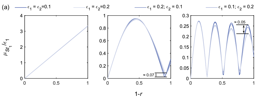
Figure 4: Relative spatial response of conical flame under (a) different amplitudes of excitations ($\delta=0$; left: $St_{1}=0.1,R=0.3$; middle: $St_{1}=5,R=1.6$; right: $St_{1}=10,R=0.6$) and under (b) different phase difference of two excitations ($\epsilon_{1}=\epsilon_{2}=0.1$, $St_{1}=5,R=1.2$, the superscript “$N$” denotes numerical results). $\cot\alpha=3$.

Figure 5: (a) The magnitude and phase of each term at $St_{1}$ for the conical flame front in equation (21). (b) The magnitude and phase of term combined solutions at $St_{1}$ for the conical flame front. ($St_{1}=5$, $St_{2}=8$, $\epsilon_{1}=\epsilon_{2}=0.2$, $\cot\alpha=3$.)

The underlying mechanisms of the above phenomenon are discussed below. Figure 5 (a) shows the magnitude and phase of each term in equation (21). The magnitude of the self-nonlinear solution is smaller than that of the mutual nonlinear solution (this relation depends on the modulation frequency) in specific frequencies of excitations. Their phases are the same ($\chi_{\rm I,1,1,1}=\chi_{\rm I,1,2,2}$)(this relation is insensitive to the modulation frequency), as they both come from the third-order PDEs . More interestingly, $\xi_{1}$, $\xi_{\rm{I},1,1,1}$ and $\xi_{\rm{I},1,2,2}$ are not affected by the phase difference $\delta$ of two interferences, thus ${\xi_{S{t_{1}}}}$ is also insensitive to $\delta$ (see figure 4 (b)). The terms for $\xi_{1}$ and $\xi_{1,1,1}$ are easy to understand because they are only influenced by the excitation at $St_{1}$. The latter induces $\xi_{\rm{I},1,1,1}$, which is naturally insensitive to $\delta$. $\xi_{1,2,2}$, dominated by excitations not only at $St_{1}$ but also at $St_{2}$, induces $\xi_{\rm{I},1,2,2}$, which is also not affected by $\delta$. This characteristic has been validated by related experimental research [41], which proves the credibility of the modelling results here. Due to the above traits, the following results are based on $\delta=0$. Figure 5 (b) shows that due to the introduction of nonlinear solutions (both the self-nonlinear and mutual-nonlinear terms, where $\xi_{PL,St_{1}}=\epsilon_{1}\xi_{1}$, $\xi_{PN,St_{1}}=\epsilon_{1}\xi_{1}+{\epsilon_{1}}^{3}\xi_{\rm{I},1,1,1}$ and $\xi_{FN,St_{1}}={\xi_{S{t_{1}}}}$), the magnitude and phase of the flame spatial response at $St_{1}$ are corrected based on the linear result. Among them, with the increase of downstream distance, the amplitude of flame wrinkle decreases, and the phase step phenomenon is suppressed.

Figure 6: The relative value $H_{St_{1}}\left(r\right)$ of mutual-nonlinear and self-nonlinear amplitudes for the V-shaped flame (a) $\sim$ (c) and for the conical flame (d) $\sim$ (f) at (a) (d) $St_{1}$ = 1, (b) (e) $St_{1}$ = 5 and (c) (f) $St_{1}$ = 9 ($H_{St_{1}}\left(r\right)=\mu_{\rm{I},1,2,2}\left(r\right)-\mu_{\rm{I},1,1,1}\left(r\right)$, $R=St_{2}/St_{1}$, $\cot\alpha=3$, ${\it\Omega_{b}}=0$).

To visually compare the nonlinear effects of excitations at $St_{1}$ and $St_{2}$ on the spatial response at $St_{1}$ (which demonstrate the ability to correct for linear results), the relative value $H_{St_{1}}\left(r\right)$ of mutual-nonlinear and self-nonlinear amplitudes is directly defined as $\mu_{\rm{I},1,2,2}\left(r\right)-\mu_{\rm{I},1,1,1}\left(r\right)$, because their corresponding phases are always identical. For the V-shaped flame (see figure 6 (a) $\sim$ (c)) and conical flame (see figure 6 (d) $\sim$ (f)), it can be found that the mutual nonlinear amplitude is smaller than the self-nonlinear term only in a very small range of low forced frequencies. As $St_{2}$ increases, $\mu_{\rm{I},1,2,2}\left(r\right)$ exhibits a steady peak, with a monotonic increase followed by a decrease. This peak represents the strongest effect of perturbation with frequency $St_{2}$ in suppressing the amplitude of flame wrinkles at $St_{1}$. With increasing $St_{2}$, $\mu_{\rm{I},1,2,2}\left(r\right)$ is usually larger than $\mu_{\rm{I},1,1,1}\left(r\right)$, especially at the spatial location approaching the flame tip. It should be noticed that regardless of $St_{1}$, the steady peak of the mutual-nonlinear solution always exists and corresponds to the case of $St_{2}\approx 3.5$ in the case of V-shaped flame, which is determined by the relation between $St$ and $K$. The nonlinear solution usually varies monotonically with the modulation frequency or $u_{c}$ ($u_{c}\in\left[\bar{u},c\right]$, $c$ is the speed of sound) [16]. The impact of flame kinematic restoration causes smaller length-scale wrinkles (associated with smaller $u_{c}$ and larger $St$) to be more prone to destruction, leading to an increase in flame kinematic response for dissipation. However, there is a negative correlation between them (see figure 2), resulting in a stable peak of the nonlinear response. This is further validated by the conical flame. The stable peak of mutual nonlinear solution in the conical flame, which is approximately $St_{2}\approx 3.85$, undergoes a modification due to the quantitative variation in the correlation between modulation frequency and $K$ when compared to the V-shaped flames.

IV Flame global nonlinear response

One can determine the HRR of a premixed flame by quantifying the perturbation area resulting from flame front-tracking [42]. However, the presence of excitations alters the time-average ensemble kinematics of the flame [43], which in turn affects the effective displacement speed of the flame and influences its HRR. It is important to note that this phenomenon, not previously documented in the literature, suggests that excitation with frequency $St_{2}$ can impact the global response of the flame. Specifically, the flame displacement speed $S_{\rm eff,disp}$ used in the HRR calculation is altered compared to that of a steady flame.

Following this point, based on equation (4), the flame displacement speed accounting for the time-averaged flame dynamics is given by

$${S_{{\rm{eff,disp}}}}\left(r\right)=\left\langle-\frac{{\partial\xi/\partial t-u}}{{{{\left[{1+{{\left({\partial\xi/\partial r}\right)}^{2}}}\right]}^{1/2}}}}\right\rangle$$ (23)

where, “$\left\langle{}\right\rangle$” denotes the time-averaged properties. One can obtain $\xi$ either through numerical approach or asymptotic analysis (as shown in Equation (17)). Notably, in order to ensure the accuracy of the results, the numerical approach is preferred. This is because only $\xi_{St_{1}}$ in asymptotic analysis is verified by numerical solutions, while $\xi$ is not.

A correction method for the instantaneous HRR calculation which accounts for the change in effective flame displacement speed is as follows:

$$\dot{\cal Q}\left(t\right)=\int_{r}{\rho{h_{R}}{S_{{\rm{eff}},{\rm{disp}}}}}\left(r\right){\left[{1+{{\left({\frac{{\partial\xi\left({r,t}\right)}}{{\partial r}}}\right)}^{2}}}\right]^{1/2}}r\rm{d}r,$$ (24)

herein, the term ${\left[{1+{{\left({\partial\xi/\partial r}\right)}^{2}}}\right]^{1/2}}$ is the same as the left-hand side (LHS) of equation (19) but with a different physical meaning. It represents the different instantaneous slopes of the flame front at different spatial locations, called the local flame front gradient.

The steady HRR is also obtained as follows,

$$\overline{\dot{\cal Q}}=\int_{r}{\rho{h_{R}}{S_{L}}}{\left[{1+{{\left({\frac{{\partial{\xi_{0}}}}{{\partial r}}}\right)}^{2}}}\right]^{1/2}}r\rm{d}r$$ (25)

The normalised instantaneous HRR fluctuation is given by

$${q^{\prime}}\left(t\right)=\left[{\dot{\cal Q}\left(t\right)-\overline{\dot{\cal Q}}}\right]/\overline{\dot{\cal Q}}$$ (26)

Perfectly premixed flames are considered in this work such that the disturbance in $\rho$ and $h_{R}$ can be neglected, thus $\rho$ and $h_{R}$ vanish in equation (26).

The results of asymptotic analysis at $St_{1}$ are plausible enough to allow us to quantify the global response at $St_{1}$ by substituting the expression for $\xi_{St_{1}}$ (equation (21)) into equation (24), as previously mentioned. Whereas, in certain special cases, the flame response at $\left|mSt_{2}-nSt_{1}\right|$ (when $m\neq 0$ and $n\neq 1$) affects that at $St_{1}$. For instance, when $St_{2}=2St_{1}$ or $St_{2}=St_{1}$, the response at $\left|St_{2}-St_{1}\right|$ or $St_{2}$ contributes to that at $St_{1}$, which is common, but cannot be captured by asymptotic analysis at $St_{1}$. Therefore, the global response at $St_{1}$ is derived from the numerical results. However, it should be noted that the majority of the response at $St_{1}$ can be fully and exactly explained by asymptotic analysis. To achieve complete and accurate capture of the flame response, linearisation of the flame displacement speed and the local flame front gradient is not considered.

Since the HRR is a nonlinear function of the two excitation frequencies, it contains all possible linear combinations of $St_{1}$ and $St_{2}$. By using the double Fourier series expansion, ${q^{\prime}}$ is expressed as

$${q^{\prime}}=\sum\limits_{m}{\sum\limits_{n}{{{\hat{q}}_{mS{t_{1}}+nS{t_{2}}}}\cos\left[{\left({mS{t_{1}}+nS{t_{2}}}\right)t+{\varphi_{mS{t_{1}}+nS{t_{2}}}}}\right]}}$$ (27)

where, $m,n\in\mathbb{Z}$; ${{\hat{q}}}$ and ${\varphi}$ are amplitudes and phases, and are a function of perturbation frequency and amplitude.

Following the main focus of this work, only the numerical results at $St_{1}$ are extracted from equation (27), and the expression for the flame describing function of two inputs (FDF-TI) is as follows:

$$\begin{split}{{F}_{S{t_{1}}}}={\frac{{{{\hat{q}}_{S{t_{1}}}}{e^{{\rm{i}}{\varphi_{S{t_{1}}}}}}}}{{{\epsilon_{1}}}}}\end{split}$$ (28)

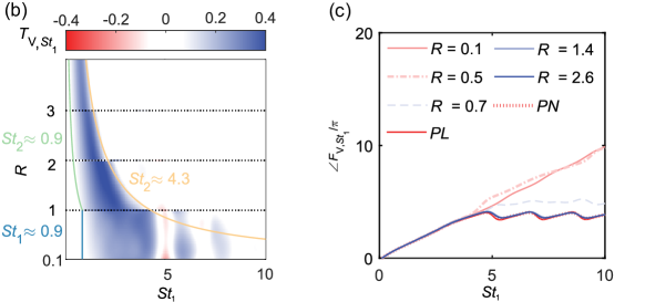
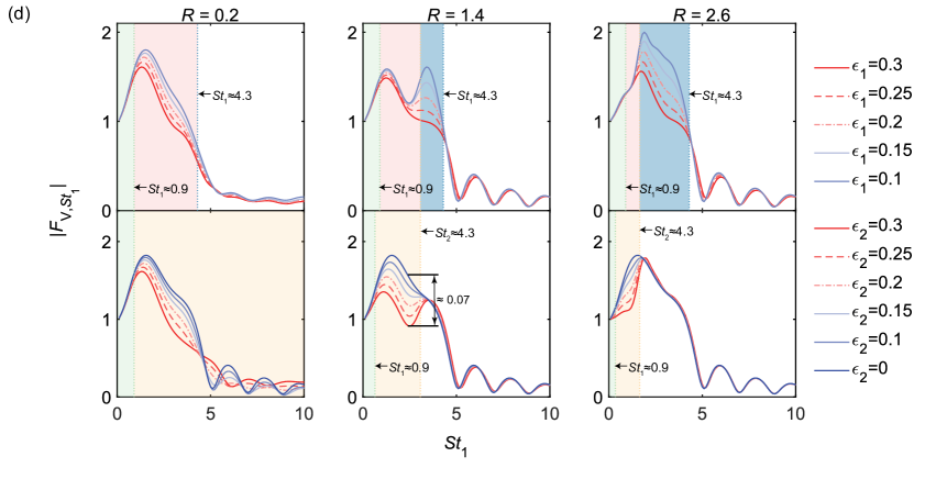
Figure 7: (a) The FDF-TI gain of the V-shaped flame at $St_{1}$ is dependent on two forced frequencies; “$\circ$” represents a localized maximum, which has a value greater than 1 and is referred to as a “bump”. (b) The two input frequencies have an impact on the relative value ${T}_{{\rm V},St_{1}}$. (c) The FDF-TI phase is influenced by perturbation frequencies in specific cases. “$PL$” represents the purely linear solution, where nonlinearities in flame kinematic restoration, flame displacement speed, and local front gradient are all neglected. “$PN$” represents the partial nonlinear solution, where all nonlinearities induced from perturbation at $St_{2}$ are neglected. ($\epsilon_{1}=0.2,\epsilon_{2}=0.1$; $R=St_{2}/St_{1}$; $\cot\alpha=3$; ${\it\Omega_{b}}=0$.) (d) The FDF-TI gain varies for different two forced amplitudes. The top frames show $\epsilon_{2}=0.2$, while the bottom frames show $\epsilon_{1}=0.2$. The dash green lines indicate when $St_{1}$ or $St_{2}$ is approximately 0.9, while the dash blue and yellow lines indicate when $St_{1}$ and $St_{2}$ are approximately 4.3, respectively. ($\cot\alpha=3$; ${\it\Omega_{b}}=0$.)

Figure 7 shows the dependence of the FDF-TI of the V-shaped flame on the dual-frequency excitation. The results depicted in figure 7 (a) demonstrate that the gain of the flame response exhibits typical characteristics of a V-shaped flame (for associated experimental results, readers can refer to [44]), where the FDF-TI gain is larger than unity within the low excitation frequency range, indicating that the flame acts as an amplifier for disturbances. When the disturbance at $St_{2}$ is considered, features with gains greater than unity are altered significant, and varies with the variation of the frequency $St_{2}$, and especially at $R\in\left(1,2\right]$, where the single peak becomes multiple bumps. There are even three local maxima when $St_{2}$ is twice as large as $St_{1}$. In general, in non-experimental studies, the V-shaped flame has a single peak with a value above 1 [42], with the corresponding frequency considered the “resonant frequency” of this flame [45]. The flame gain exceeding unity plays a key role in the potential not only for intrinsic thermoacoustic (ITA) instability [46, 47], but also for the analysis of the formation of thermoacoustic instability.

Figure 7 (b) fully reflects the role of the perturbation at $St_{2}$ in the FDF-TI by introducing the parameter $T_{{\rm V},St_{1}}$. The value of $T_{{\rm V},St_{1}}$ is given by $\left|{{{F}^{PN}_{{\rm{V,}}S{t_{1}}}}}\right|-\left|{{{F}^{FN}_{{\rm{V,}}S{t_{1}}}}}\right|$, where the superscript “$FN$” represents the full nonlinear solution, including all nonlinearities caused by the two input excitations (equalling the cases of $R\neq 0$), and the superscript “$PN$” represents the partial nonlinear solution, in which all nonlinearities induced from perturbation at $St_{2}$ are neglected (equalling the cases of $R=0$). A positive value of $T_{{\rm V},St_{1}}$ indicates that the perturbation at $St_{2}$ weakens the flame response magnitude. Two boundary lines define a region within which the difference value $T_{{\rm V},St_{1}}$ is significant, while outside of which it is negligible, excluding some special conditions. The left boundary accounts for the threshold of frequency in the flame linear response, while the right boundary accounts for the threshold of frequency in the saturation of flame nonlinear response. The low-order asymptotic analysis shows that $\xi_{{\rm I},1,2,2}$ in equation (21) obviously controls the properties of FDF-TI gain. When the modulation frequency is sufficiently small ($St<0.9$), the role of $\xi_{{\rm I},1,2,2}$ is suppressed, and the gain is insensitive to the perturbation at $St_{2}$. With the development of $St_{2}$, $\xi_{{\rm I},1,2,2}$ significantly alters the gain characteristics of the FDF-TI due to the presence of a distinct nonlinear flame response. As mentioned earlier, the negative correlation between $St$ and $K$ dominates the value of $\xi_{{\rm I},1,1,2}$, thus creating a critical frequency (4.3) beyond which the effect of the perturbation at $St_{2}$ on the gain rapidly diminishes and the flame enters the response saturation region. In some special cases, the effect of the perturbation at $St_{2}$ on the FDF-TI outside the critical frequency boundary is evident, especially for small $R$. Furthermore, whenever $R$ transitions to a natural number (e.g., 1, 2, 3), there is a noticeable jump in the value of $T_{\rm V}$, as some additional gain occurs in these special cases. These so-called “errors” occur because the flame response at $\left|mSt_{2}-nSt_{1}\right|$ (when $m\neq 0$ and $n\neq 1$) affects that at $St_{1}$. For instance, when $St_{2}=2/3St_{1}$ or $St_{2}=2St_{1}$, the response at $\left|3St_{2}-St_{1}\right|$ or $\left|St_{2}-St_{1}\right|$ contributes to that at $St_{1}$. These new contributions are not included in the scope of the original flame response at $St_{1}$ and can not be described by the corresponding asymptotic analysis.

In figure 7 (c), it can be observed that the phase changes exhibit more regularity in comparison to the intricate behaviours of the FDF-TI gain. The impact of the perturbation at $St_{2}$ is confined to the high-frequency range of $St_{1}$ and is only noticeable when $St_{2}<St_{1}$. This is due to the inverse relation between $St$ and $K$, resulting in $K_{2}>K_{1}$ when $St_{2}<St_{1}$. As $K$ increases, $u_{c}$ decreases steadily, which restricts the propagation of acoustic disturbance and amplifies the response of the FDF-TI phase to excitations.

By analysing the amplitude variation of the two excitations, as shown in figure 7 (d), the nonlinear gain characteristics are further determined. The destructive features become more pronounced with increasing perturbation amplitude. Particularly, when subjected to the perturbation at $St_{1}$ with $\epsilon_{1}=0.2$, the HRR gain at $St_{1}$ attenuates by more than 40 % compared to a single-frequency input after introducing a perturbation at $St_{2}$ with $\epsilon_{2}=0.3$ (see the case of $R=1.4$). This is due to the fact that the enhancement of large-amplitude perturbations readily produces small-scale wrinkles, which are easily smoothed back by the flame motion, thus reducing the gain. The above phenomenon is limited to the effective region enclosed by two previously identical boundary frequencies (0.9 and 4.3). The effective region can be used to explain the mechanism of multi-bump phenomenon formation of the FDF-TI’s gain. For the single peak cases ($R<1$ and $R>2$), the behaviours of the FDF-TI gain are similar, but the underlying mechanism is different. When $R<1$, the peak is located in the effective region of frequencies $St_{1}$ and $St_{2}$, and is therefore sensitive to both amplitudes of two excitations. However, when $R>2$, the peak is located in the effective region of $St_{1}$ but outside the effective region of $St_{2}$, so it is mainly sensitive to perturbations at $St_{1}$ but not at $St_{2}$. For the double bumps case ($1<R<2$), the first peak lies in the effective region of $St_{2}$ and is dominated by $St_{2}$. Although in this case the first peak is also controlled by the perturbation at $St_{1}$, saturation of the flame nonlinear response with respect to the perturbation amplitude occurs. Therefore, the perturbation at $St_{1}$ has less influence on this peak. The formation of the latter peak in the double bumps case is similar to the previous case of $R>2$, which is controlled only by the perturbation at $St_{1}$. In the case of three bumps ($R=2$, see figure7 (a)), the first two bumps are formed for similar reasons as in the case of the previous two bumps, with the third peak clearly associated with frequency $\left|St_{2}-St_{1}\right|$. When $R=2$, $\left|St_{2}-St_{1}\right|$ becomes $St_{1}$, contributing to the external gain in flame response at $St_{1}$.

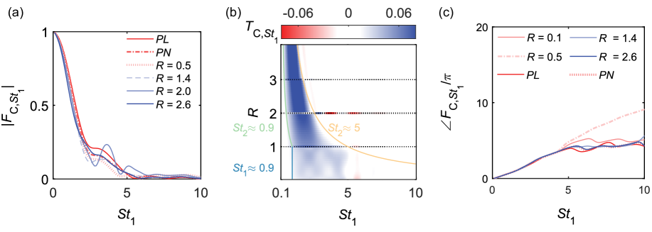
Figure 8: (a) The FDF-TI gain of conical flame in some specific cases. (b) Effect of two input frequencies on the relative value $T_{{\rm C},St_{1}}$. (c) The FDF-TI phase in some specific cases. ($\epsilon_{1}=0.1,\epsilon_{2}=0.2$; $\cot\alpha=3$.)

The results of the perturbation at $St_{2}$ on the FDF-TI of the conical flame are also presented. With the exception of specific instances (e.g., $R=2$ in figure 8 (a)), the introduction of perturbations at $St_{2}$ significantly reduces the FDF-TI gain compared to the purely linear (“$PL$”) or partially nonlinear (“$PN$”) cases. However, as nonlinear factors such as flame displacement speed and local flame gradient become more prominent with increasing modulation frequency, this leads to an amplitude enhancement of the full nonlinear response in the high range of $St_{1}$.

The role of $St_{2}$ in the flame amplitude is fully determined in figure 8 (b), where two boundary lines indicate an similarly effective region with the same physical meaning as in the V-shaped flame case. The threshold value of the linear response of the flame is not affected by the relation between the forcing frequency and $K$ (it corresponds to $K=1$) and is also equal to 0.9 for conical flames. Whereas, the saturation threshold frequency 5 in the nonlinear response of the flame changes and corresponds to the same $K$ as in the case of V-shaped flames, as shown in figure 2. This is because the nonlinear effect of the perturbation on the FDF-TI gain usually varies monotonically with $St$ or $u_{c}$, but here it is governed by the negative correlation between $St$ and $u_{c}$, and hence there exists a specific $K$ to balance out the competition between them. The flame response gain in the high frequency range of $St_{1}$ decreases, but does not exhibit significant characteristics similar to the V-shaped flame response. This can be attributed to the fact that nonlinear factors are more prominent when the spatial location is far from the flame holder. For conical flames, the spatial weighting of the FDF-TI calculations tapers off from the anchor point to the tip, significantly weakening the nonlinear response. Some special cases are observed where the effect of perturbations at $St_{2}$ on the gain lies outside the effective region and is formed in the same way as in the case of V-shaped flames.

Figure 8 (c) illustrates the impact of perturbation at $St_{2}$ on the FDF-TI phase. The phase is notably influenced by $St_{2}$, particularly in the high-frequency range of $St_{1}$ and low $R$ situations. As the $R$ increases, the phase trajectory tends to approach that of “$PL$” case. Under the same conditions, the phase consistency of different $St_{2}$ in the V-shaped flame is better. According to results in figure 2, the value of $K$ for the conical flame is larger than that for the V-shaped flame as the forced frequency increases. This monotonically corresponds to a smaller $u_{c}$, constraining the propagation of acoustic perturbation and thus magnifying the discrepancy in the phase response to excitations.

V Conclusion

This paper examined the laminar flame nonlinear response characteristics by imposing simultaneously at two distinct frequencies denoted $St_{1}$ and $St_{2}$. The nonlinear features for the flame’s spatial and global responses were obtained through a low-order asymptotic analysis based on the $G$-equation model, which retained terms up to the third order in normalised excitation amplitude. To ensure the accuracy of the analytical solution and complement it, numerical flame front tracing methods that relied on the $G$-equation model were used.

An explicit mechanism by which the perturbation at $St_{2}$ suppresses the flame kinematics at $St_{1}$ is shown. From an asymptotic analytical point of view, the third-order mutual nonlinear term induced by the perturbations at $St_{1}$ and $St_{2}$ attenuates the folds in the flame front tracking compared to the single-frequency response. In particular, as $St_{2}$ increases, there is a steady peak in the effect of mutual nonlinear effects on the spatial response, first increasing monotonically and then decreasing. The reason is that the nonlinear result typically changes in a consistent manner with the modulation frequency $St$ or propagation speed of the flow disturbance $u_{c}$. The presence of flame kinematic restoration results in a higher likelihood of wrinkles on smaller length scales (associated with smaller $u_{c}$ and larger $St$) being eliminated, resulting in an increase in the dissipative flame kinematic response. Thus, as $St$ increases, the positive correlation between $u_{c}$ and $St$ leads to the nonmonotonicity described above. Based on the results of the flame spatial wrinkling, the heat release rate (HRR) response is calculated and the two boundaries are revealed, thus extracting the effective region where the perturbation at $St_{2}$ plays an important role in the HRR at $St_{1}$. The left boundary line represents the frequency threshold in the linear response, while the right boundary line dominated by the negative correlation between $u_{c}$ and $St$, indicates the frequency threshold at which the nonlinear response of the flame saturates. When $St_{2}$ is located within this effective region, it significantly alters the character of the HRR gain, including features beyond unity in the V-shaped flame, which is critical not only for potential intrinsic thermoacoustic (ITA) instabilities, but also for analyzing the formation of thermoacoustic instabilities. In addition, the perturbation at $St_{2}$ increases its amplitude variation greatly disrupting the gain of the nonlinear response. This is because the enhancement of large amplitude perturbations can easily produce small-scale wrinkles that can be easily smoothed out by the flame kinematics, thus reducing the gain. Particularly, when subjected to a perturbation at $St_{1}$ with a normalized amplitude of 0.2, the HRR gain at $St_{1}$ attenuates by more than 40 % compared to a single-frequency input after introducing a perturbation at $St_{2}$ with a normalized amplitude of 0.3. This offers the possibility to suppress instabilities by introducing additional excitations to the flame at carefully chosen frequencies.

VI Derivation of asymptotic solutions

It is possible to apply the asymptotic expansion (17) and Taylor expansion (19) to the dynamic flame front equation (4) and match terms with the same order. The PDEs of different flames have similar forms. For the sake of brevity, only the governing equations of each order of the conical flame front are given. For the linear terms, they are

$$\frac{{\partial{\xi_{1}}}}{{\partial t}}-\frac{1}{2}\sin 2\alpha\frac{{\partial{\xi_{1}}}}{{\partial r}}={{\mathcal{C}}_{1}}\left({r,t}\right)$$ (29)

$$\frac{{\partial{\xi_{2}}}}{{\partial t}}-\frac{1}{2}\sin 2\alpha\frac{{\partial{\xi_{2}}}}{{\partial r}}={{\mathcal{C}}_{2}}\left({r,t}\right)$$ (30)

The forms of the self-nonlinear terms are

$$\frac{{\partial{\xi_{1,1}}}}{{\partial t}}-\frac{1}{2}\sin 2\alpha\frac{{\partial{\xi_{1,1}}}}{{\partial r}}=-\frac{1}{2}{\sin^{4}}\alpha{\left({\frac{{\partial{\xi_{1}}}}{{\partial r}}}\right)^{2}}$$ (31)

$$\frac{{\partial{\xi_{2,2}}}}{{\partial t}}-\frac{1}{2}\sin 2\alpha\frac{{\partial{\xi_{2,2}}}}{{\partial r}}=-\frac{1}{2}{\sin^{4}}\alpha{\left({\frac{{\partial{\xi_{2}}}}{{\partial r}}}\right)^{2}}$$ (32)

$$\frac{{\partial{\xi_{1,1,1}}}}{{\partial t}}-\frac{1}{2}\sin 2\alpha\frac{{\partial{\xi_{1,1,1}}}}{{\partial r}}=-{\sin^{4}}\alpha\frac{{\partial{\xi_{1}}}}{{\partial r}}\frac{{\partial{\xi_{1,1}}}}{{\partial r}}$$ (33)

$$\frac{{\partial{\xi_{2,2,2}}}}{{\partial t}}-\frac{1}{2}\sin 2\alpha\frac{{\partial{\xi_{2,2,2}}}}{{\partial r}}=-{\sin^{4}}\alpha\frac{{\partial{\xi_{2}}}}{{\partial r}}\frac{{\partial{\xi_{2,2}}}}{{\partial r}}$$ (34)

and the three mutual-nonlinear terms are

$$\frac{{\partial{\xi_{1,2}}}}{{\partial t}}-\frac{1}{2}\sin 2\alpha\frac{{\partial{\xi_{1,2}}}}{{\partial r}}=-{\sin^{4}}\alpha\frac{{\partial{\xi_{1}}}}{{\partial r}}\frac{{\partial{\xi_{2}}}}{{\partial r}}$$ (35)

$$\frac{{\partial{\xi_{1,2,2}}}}{{\partial t}}-\frac{1}{2}\sin 2\alpha\frac{{\partial{\xi_{1,2,2}}}}{{\partial r}}=-{\sin^{4}}\alpha\left({\frac{{\partial{\xi_{1}}}}{{\partial r}}\frac{{\partial{\xi_{2,2}}}}{{\partial r}}+\frac{{\partial{\xi_{2}}}}{{\partial r}}\frac{{\partial{\xi_{1,2}}}}{{\partial r}}}\right)$$ (36)

$$\frac{{\partial{\xi_{1,1,2}}}}{{\partial t}}-\frac{1}{2}\sin 2\alpha\frac{{\partial{\xi_{1,1,2}}}}{{\partial r}}=-{\sin^{4}}\alpha\left({\frac{{\partial{\xi_{1}}}}{{\partial r}}\frac{{\partial{\xi_{1,2}}}}{{\partial r}}+\frac{{\partial{\xi_{2}}}}{{\partial r}}\frac{{\partial{\xi_{1,1}}}}{{\partial r}}}\right)$$ (37)

Those equations are solved sequentially based on the boundary condition equation (5). For the linear terms, these are

$${\xi_{1}}\left({r,t}\right)=\frac{\sin\left[St_{1}\left(-1+r+\Gamma t\right)/\Gamma\right]-\sin\left[St_{1}\left(\cot\alpha K_{1}\left(-1+r\right)+t\right)\right]}{St_{1}\left(-1+\Gamma\cot\alpha K_{1}\right)}$$ (38)

where, $\Gamma=\cos\alpha\sin\alpha$,

$${\xi_{2}}\left({r,t,\delta}\right)=\frac{\sin\left[\delta-St_{2}\left(\cot\alpha K_{2}\left(-1+r\right)+t\right)\right]-\sin\left[St_{2}\left(1+\Gamma\delta-r-\Gamma t\right)/\Gamma\right]}{St_{2}\left(-1+\Gamma\cot\alpha K_{2}\right)}$$ (39)

The specific solutions for the rest of the terms are too complex and, to improve readability, these results are omitted. To be honest, we prefer to focus on the frequencies of the responses, which visually illustrate the interaction path of dual-frequency perturbations on the flame response. Therefore, the corresponding concise expressions are sufficient for us.

For linear solutions, they can be rewritten as

$${\xi_{1}}\left({r,t}\right)={{\mu_{1}}\left(r\right)}\cos\left[{S{t_{1}}t+{\chi_{1}}\left(r\right)}\right]$$ (40)

$${\xi_{2}}\left({r,t,\delta}\right)={{\mu_{2}}\left(r,\delta\right)}\cos\left[{S{t_{2}}t+{\chi_{2}}\left(r,\delta\right)}\right]$$ (41)

The forms of self-nonlinear terms are

$$\begin{split}{\xi_{1,1}}\left({r,t}\right)&={\xi_{{\rm{I}},{\rm{1}},{\rm{1}}}}\left({r,t}\right)+{\xi_{{\rm{II}},{\rm{1}},{\rm{1}}}}\left(r\right)\\ &={{\mu_{{\rm{I}},{\rm{1}},{\rm{1}}}}\left(r\right)}\cos\left[{2S{t_{1}}t+{\chi_{{\rm{I}},{\rm{1}},{\rm{1}}}}\left(r\right)}\right]+{\mu_{{\rm{II}},{\rm{1}},{\rm{1}}}}\left(r\right)\end{split}$$ (42)

$$\begin{split}{\xi_{2,2}}\left({r,t,\delta}\right)&={\xi_{{\rm{I}},{\rm{2}},{\rm{2}}}}\left({r,t,\delta}\right)+{\xi_{{\rm{II}},{\rm{2}},{\rm{2}}}}\left(r\right)\\ &={{\mu_{{\rm{I}},{\rm{2}},{\rm{2}}}}\left(r,\delta\right)}\cos\left[{2S{t_{2}}t+{\chi_{{\rm{I}},{\rm{2}},{\rm{2}}}}\left(r,\delta\right)}\right]+{\mu_{{\rm{II}},{\rm{2}},{\rm{2}}}}\left(r\right)\end{split}$$ (43)

$$\begin{split}{\xi_{1,1,1}}\left({r,t}\right)&={\xi_{{\rm{I}},1,1,1}}\left({r,t}\right)+{\xi_{{\rm{II}},1,1,1}}\left({r,t}\right)\\ &={{\mu_{{\rm{I}},1,1,1}}\left(r\right)}\cos\left[{S{t_{1}}t+{\chi_{{\rm{I}},1,1,1}}\left(r\right)}\right]\\ &+{{\mu_{{\rm{II}},1,1,1}}\left(r\right)}\cos\left[{3S{t_{1}}t+{\chi_{{\rm{II}},1,1,1}}\left(r\right)}\right]\end{split}$$ (44)

$$\begin{split}{\xi_{2,2,2}}\left({r,t,\delta}\right)&={\xi_{{\rm{I}},2,2,2}}\left({r,t,\delta}\right)+{\xi_{{\rm{II}},2,2,2}}\left({r,t,\delta}\right)\\ &={{\mu_{{\rm{I}},2,2,2}}\left(r,\delta\right)}\cos\left[{S{t_{2}}t+{\chi_{{\rm{I}},2,2,2}}\left(r,\delta\right)}\right]\\ &+{{\mu_{{\rm{II}},2,2,2}}\left(r,\delta\right)}\cos\left[{3S{t_{2}}t+{\chi_{{\rm{II}},2,2,2}}\left(r,\delta\right)}\right]\end{split}$$ (45)

and the three mutual-nonlinear terms are

$$\begin{split}{\xi_{1,2}}\left({r,t,\delta}\right)&={\xi_{{\rm{I}},{\rm{1}},{\rm{2}}}}\left({r,t,\delta}\right)+{\xi_{{\rm{II}},{\rm{1}},{\rm{2}}}}\left({r,t,\delta}\right)\\ &={{\mu_{{\rm{I}},{\rm{1}},{\rm{2}}}}\left(r,\delta\right)}\cos\left[{\left({S{t_{1}}+S{t_{2}}}\right)t+{\chi_{{\rm{I}},{\rm{1}},{\rm{2}}}}\left(r,\delta\right)}\right]\\ &+{{\mu_{{\rm{II}},{\rm{1}},{\rm{2}}}}\left(r,\delta\right)}\cos\left[{\left|{S{t_{1}}-S{t_{2}}}\right|t+{\chi_{{\rm{II}},{\rm{1}},{\rm{2}}}}\left(r,\delta\right)}\right]\end{split}$$ (46)

$$\begin{split}{\xi_{1,1,2}}\left({r,t,\delta}\right)&={\xi_{{\rm{I}},{\rm{1}},{\rm{1}},{\rm{2}}}}\left({r,t,\delta}\right)+{\xi_{{\rm{II}},{\rm{1}},{\rm{1}},{\rm{2}}}}\left({r,t,\delta}\right)+{\xi_{{\rm{III}},{\rm{1}},{\rm{1}},{\rm{2}}}}\left({r,t,\delta}\right)\\ &={{\mu_{{\rm{I}},{\rm{1}},{\rm{1}},{\rm{2}}}}\left(r,\delta\right)}\cos\left[{S{t_{2}}t+{\chi_{{\rm{I}},{\rm{1}},{\rm{1}},{\rm{2}}}}\left(r,\delta\right)}\right]\\ &+{{\mu_{{\rm{II}},{\rm{1}},{\rm{1}},{\rm{2}}}}\left(r,\delta\right)}\cos\left[{\left({2S{t_{1}}+S{t_{2}}}\right)t+{\chi_{{\rm{II}},{\rm{1}},{\rm{1}},{\rm{2}}}}\left(r,\delta\right)}\right]\\ &+{{\mu_{{\rm{III}},{\rm{1}},{\rm{1}},{\rm{2}}}}\left(r,\delta\right)}\cos\left[{\left|{2S{t_{1}}-S{t_{2}}}\right|t+{\chi_{{\rm{III}},{\rm{1}},{\rm{1}},{\rm{2}}}}\left(r,\delta\right)}\right]\end{split}$$ (47)

$$\begin{split}{\xi_{1,2,2}}\left({r,t,\delta}\right)&={\xi_{{\rm{I}},{\rm{1}},{\rm{2}},{\rm{2}}}}\left({r,t}\right)+{\xi_{{\rm{II}},{\rm{1}},{\rm{2}},{\rm{2}}}}\left({r,t,\delta}\right)+{\xi_{{\rm{III}},{\rm{1}},{\rm{2}},{\rm{2}}}}\left({r,t,\delta}\right)\\ &={{\mu_{{\rm{I}},{\rm{1}},{\rm{2}},{\rm{2}}}}\left(r\right)}\cos\left[{S{t_{1}}t+{\chi_{{\rm{I}},{\rm{1}},{\rm{2}},{\rm{2}}}}\left(r\right)}\right]\\ &+{{\mu_{{\rm{II}},{\rm{1}},{\rm{2}},{\rm{2}}}}\left(r,\delta\right)}\cos\left[{\left({2S{t_{2}}+S{t_{1}}}\right)t+{\chi_{{\rm{II}},{\rm{1}},{\rm{2}},{\rm{2}}}}\left(r,\delta\right)}\right]\\ &+{{\mu_{{\rm{III}},{\rm{1}},{\rm{2}},{\rm{2}}}}\left(r,\delta\right)}\cos\left[{\left|{2S{t_{2}}-S{t_{1}}}\right|t+{\chi_{{\rm{III}},{\rm{1}},{\rm{2}},{\rm{2}}}}\left(r,\delta\right)}\right]\end{split}$$ (48)

where, $\mu$ ($\mu\geq 0$) and $\chi$ are functions of spatial location (they are also functions of the phase difference if $\delta$ is present in their expressions) and represent the amplitudes and phases of terms in each order equation, respectively. The subscripts “I”, “II”, and “III” (if existent) denote the properties corresponding to the first, second and third disturbance frequencies included in the solution, respectively. For the V-shaped flame, the solution forms from (40) $\sim$ (48) are the same, i.e., the same frequency (frequencies) is (are) included in the governing equations of the same order, but the specific expressions of $\mu$ and $\chi$ are different to those of the conical flame.

References

- Poinsot [2017] T. Poinsot, Prediction and control of combustion instabilities in real engines, Proc. Combust. Inst. 36, 1 (2017).
- Candel [2002] S. Candel, Combustion dynamics and control: Progress and challenges, Proc. Combust. Inst. 29, 1 (2002).
- Mori et al. [2023] Y. Mori, S. Kishiya, T. Kurosaka, and H. Gotoda, Feedback coupling and early detection of thermoacoustic combustion instability, Phys. Rev. Appl. 19, 034097 (2023).
- Radisson et al. [2019] B. Radisson, J. Piketty-Moine, and C. Almarcha, Coupling of vibro-acoustic waves with premixed flame, Phys. Rev. Fluids 4, 121201 (2019).
- Aguilar and Juniper [2020] J. G. Aguilar and M. P. Juniper, Thermoacoustic stabilization of a longitudinal combustor using adjoint methods, Phys. Rev. Fluids 5, 083902 (2020).
- Schuller et al. [2003] T. Schuller, D. Durox, and S. Candel, A unified model for the prediction of laminar flame transfer functions : comparisons between conical and V-flame dynamics, Combust. Flame 134, 21 (2003).
- Juniper [2011] M. P. Juniper, Triggering in the horizontal rijke tube: non-normality, transient growth and bypass transition, J. Fluid Mech. 667, 272 (2011).
- Fleifil et al. [1996] M. Fleifil, A. M. Annaswamy, Z. A. Ghoneim, and A. F. Ghoniem, Response of a laminar premixed flame to flow oscillations: A kinematic model and thermoacoustic instability results, Combust. Flame 106, 487 (1996).
- Dowling [1999] A. P. Dowling, A kinematic model of a ducted flames, J. Fluid Mech. 394, 51 (1999).
- Noiray et al. [2008] N. Noiray, D. Durox, T. Schuller, and S. Candel, A unified framework for nonlinear combustion instability analysis based on the flame describing function, J. Fluid Mech. 615, 139 (2008).
- Durox et al. [2009] D. Durox, T. Schuller, N. Noiray, and S. Candel, Experimental analysis of nonlinear flame transfer functions for different flame geometries, Proc. Combust. Inst. 32, 1391 (2009).
- Krediet et al. [2013] H. Krediet, C. Beck, W. Krebs, and J. Kok, Saturation mechanism of the heat release response of a premixed swirl flame using LES, Proc. Combust. Inst. 34, 1223 (2013).
- Orchini and Juniper [2016a] A. Orchini and M. P. Juniper, Flame double input describing function analysis, Combust. Flame 171, 87 (2016a).
- Lipatnikov and Chomiak [2002] A. Lipatnikov and J. Chomiak, Turbulent flame speed and thickness: phenomenology, evaluation, and application in multi-dimensional simulations, Prog. Energ. Combust. Sci. 28, 1 (2002).
- Palies et al. [2011] P. Palies, D. Durox, T. Schuller, and S. Candel, Nonlinear combustion instability analysis based on the flame describing function applied to turbulent premixed swirling flames, Combust. Flame 158, 1980 (2011).
- Jiang et al. [2022] X. Jiang, J. Li, L. Yang, and T. Liu, A nonlinearly kinematic model of the asymmetrically turbulent premixed slit flame subjected to two-way harmonic disturbances, Combust. Flame 240, 112021 (2022).
- Markstein [1964] G. Markstein, Nonsteady flame propagation (Oxford: Pergamon Press, 1964).
- Schuller et al. [2002] T. Schuller, S. Ducruix, D. D, and S. Candel, Modeling tools for the prediction of premixed flame transfer functions, Proc. Combust. Inst. 29, 107 (2002).
- Lieuwen [2005] T. Lieuwen, Nonlinear kinematic response of premixed flames to harmonic velocity disturbances, Proc. Combust. Inst. 30, 1725 (2005).
- Bellows et al. [2007] B. D. Bellows, M. K. Bobba, A. Forte, J. M. Seitzman, and T. Lieuwen, Flame transfer function saturation mechanisms in a swirl-stabilized combustor, Proc. Combust. Inst. 31, 3181 (2007).
- Balachandran et al. [2008] R. Balachandran, A. P. Dowling, and E. Mastorakos, Non-linear response of turbulent premixed flames to imposed inlet velocity oscillations of two frequencies, Flow Turbul. Combust. 80, 455 (2008).
- Lamraoui et al. [2011] A. Lamraoui, F. Richecoeur, T. Schuller, and S. Ducruix, A methodology for on the fly acoustic characterization of the feeding line impedances in a turbulent swirled combustor, J. Eng. Gas Turb. Power 133, 011504 (2011).
- Albayrak et al. [2018] A. Albayrak, T. Steinbacher, T. Komarek, and W. Polifke, Convective scaling of intrinsic thermo-acoustic eigenfrequencies of a premixed swirl combustor, J. Eng. Gas Turb. Power 140, 041510 (2018).
- Haeringer et al. [2019] M. Haeringer, M. Merk, and W. Polifke, Inclusion of higher harmonics in the flame describing function for predicting limit cycles of self-excited combustion instabilities, Proc. Combust. Inst. 37, 5255 (2019).
- Haeringer and Polifke [2019] M. Haeringer and W. Polifke, Time-domain bloch boundary conditions for efficient simulation of thermoacoustic limit cycles in (can-)annular combustors, J. Eng. Gas Turb. Power 141, 121005 (2019).
- Tathawadekar et al. [2021] N. Tathawadekar, N. A. K. Doan, C. F. Silva, and N. Thuerey, Modeling of the nonlinear flame response of a bunsen-type flame via multi-layer perceptron, Proc. Combust. Inst. 38, 6261 (2021).
- Han et al. [2016] X. Han, J. Yang, and J. Mao, LES investigation of two frequency effects on acoustically forced premixed flame, Fuel 185, 449 (2016).
- Moeck and Paschereit [2012] J. P. Moeck and C. O. Paschereit, Nonlinear interactions of multiple linearly unstable thermoacoustic modes, Int. J. Spary Combust. 4, 1 (2012).
- Shin and Lieuwen [2012] D. H. Shin and T. Lieuwen, Flame wrinkle destruction processes in harmonically forced, laminar premixed flames, Combust. Flame 159, 3312 (2012).
- Hemchandra et al. [2011] S. Hemchandra, N. Peters, and T. Lieuwen, Heat release response of acoustically forced turbulent premixed flames-role of kinematic restoration, Proc. Combust. Inst. 33, 1609 (2011).
- Preetham et al. [2008] R. Preetham, H. Santosh, and T. Lieuwen, Dynamics of laminar premixed flames forced by harmonic velocity disturbances, J. Propul. Power 24, 1390 (2008).
- Birbaud et al. [2006] A. Birbaud, D. Durox, and S. Candel, Upstream flow dynamics of a laminar premixed conical flame submitted to acoustic modulations, Combust. Flame 146, 541 (2006).
- Karimi et al. [2009] N. Karimi, M. J. Brear, S. H. Jin, and J. P. Monty, Linear and non-linear forced response of a conical, ducted, laminar premixed flame, Combust. Flame 156, 2201 (2009).
- Yang et al. [2021] Y. Yang, Y. Fang, L. Zhong, Y. Xia, T. Jin, J. Li, and G. Wang, DMD analysis for velocity fields of a laminar premixed flame with external acoustic excitation, Exp. Therm. Fluid Sci. 123, 110318 (2021).
- Blanchard et al. [2015] M. Blanchard, T. Schuller, D. Sipp, and P. J. Schmid, Response analysis of a laminar premixed M-flame to flow perturbations using a linearized compressible navier-stokes solver, Phys. Fluids 27, 043602 (2015).
- Steinbacher and Polifke [2022] T. Steinbacher and W. Polifke, Convective velocity perturbations and excess gain in flame response as a result of flame-flow feedback, Fluids 7 (2022).
- Jiang and Peng [2000] G.-S. Jiang and D. Peng, Weighted eno schemes for hamilton–jacobi equations, SIAM J. Sci. Comput. 21, 2126 (2000).
- Shu [2009] C. W. Shu, High order weighted essentially nonoscillatory schemes for convection dominated problems, SIAM Rev. 51, 82 (2009).
- Orchini and Juniper [2016b] A. Orchini and M. P. Juniper, Linear stability and adjoint sensitivity analysis of thermoacoustic networks with premixed flames, Combust. Flame 165, 97 (2016b).
- Shanbhogue et al. [2009] S. Shanbhogue, D.-H. Shin, S. Hemchandra, D. Plaks, and T. Lieuwen, Flame-sheet dynamics of bluff-body stabilized flames during longitudinal acoustic forcing, Proc. Combust. Inst. 32, 1787 (2009).
- Zheng et al. [2022] J. Zheng, L. Li, G. Wang, L. Xu, S. Wang, X. Xia, and F. Qi, The response of a conical flame to a dual-frequency excitation, INTER-NOISE and NOISE-CON Congress and Conference Proceedings, InterNoise22, Glasgow, Scotland 12, 4249 (2022).
- Schuller et al. [2020] T. Schuller, T. Poinsot, and S. Candel, Dynamics and control of premixed combustion systems based on flame transfer and describing functions, J. Fluid Mech. 894, P1 (2020).
- Acharya and Lieuwen [2020] V. Acharya and T. C. Lieuwen, Non-monotonic flame response behaviors in harmonically forced flames, Proc. Combust. Inst. 38, 6043 (2020).
- Durox et al. [2005] D. Durox, T. Schuller, and S. Candel, Combustion dynamics of inverted conical flames, Proc. Combust. Inst. 30, 1717 (2005).
- Kedia et al. [2011] K. S. Kedia, H. M. Altay, and A. F. Ghoniem, Impact of flame-wall interaction on premixed flame dynamics and transfer function characteristics, Proc. Combust. Inst. 33, 1113 (2011).
- Hao and Semperlotti [2022] H. Hao and F. Semperlotti, Instabilities of intrinsic thermoacoustic modes in a thermoacoustic waveguide with anechoic terminations, Phys. Rev. B 106, 094304 (2022).
- Silva [2023] F. Silva, Intrinsic thermoacoustic instabilities, Prog. Energ. Combust. Sci. 95 (2023).