Active-travel modelling: a methodological approach to networks for walking and cycling commuting analysis.

Abstract

Walking and cycling, commonly referred to as active travel, have become integral components of modern transport planning. Recently, there has been growing recognition of the substantial role that active travel can play in making cities more liveable, sustainable and healthy, as opposed to traditional vehicle-centred approaches. This shift in perspective has spurred interest in developing new data sets of varying resolution levels to represent, for instance, walking and cycling street networks. This has also led to the development of tailored computational tools and quantitative methods to model and analyse active travel flows.

In response to this surge in active travel-related data and methods, our study develops a methodological framework primarily focused on walking and cycling as modes of commuting. We explore commonly used data sources and tools for constructing and analysing walking and cycling networks, with a particular emphasis on distance as a key factor that influences, describes, and predicts commuting behaviour. Our ultimate aim is to investigate the role of different network distances in predicting active commuting flows.

To achieve this, we analyse the flows in the constructed networks by looking at the detour index of shortest paths. We then use the Greater London Area as a case study, and construct a spatial interaction model to investigate the observed commuting patterns through the different networks. Our results highlight the differences between chosen data sets, the uneven spatial distribution of their performance throughout the city and its consequent effect on the spatial interaction model and prediction of walking and cycling commuting flows.

1 Introduction

Urban mobility, a key component of urban dynamics, intersects with various areas of urban life including economy, environment, and social structures. This critical aspect involves the movement of people and goods within urban areas, and its efficiency and sustainability directly influence the overall functioning of cities. Given its significance, it is crucial to acquire knowledge and understanding that help plan and develop improved mobility networks. This represents an ongoing challenge, as both transport methods and human mobility patterns continue to evolve.

An essential aspect of urban mobility is commuting, which is defined as the regular travel between residence and work places. Observing trends in commuting patterns can provide valuable insights into broader shifts in urban mobility. Nowadays, there is an increased focus on small-scale movement, primarily through cycling and walking. These modes of transportation are often grouped under the term "active-travel". Contemporary planning practices accentuate their importance for reasons of health, sustainability, and safety.

While active travel currently represents a moderate share of commuting methods in England, with about 10% [35], this figure is projected to increase. The rise in active travel not only signifies potential reductions in air and noise pollution due to less reliance on cars, but also implies urban redesign opportunities. The decrease in space required for parking and driving could allow for expanded green areas, and increased housing, leisure and commercial spaces [18]. Given the current context of rising living and transport costs and global supply chain disruptions, active travel represents a practical and cost-effective transport alternative. Therefore, gaining a better understanding of the active travel flow patterns could help us adapt to these trends and meet the evolving needs of the population.

In this paper, we conduct a methodological analysis to study active travel. The study compares different walking and cycling networks to investigate how different models predict real-world flows. The findings of this research have tangible implications for policymakers and urban developers. By providing a more accurate understanding of active travel flows, the results can assist in the formulation of strategies that facilitate and promote walking and cycling.

The paper is structured into three main sections: Networks, Routing, and Modelling. In the first section, the focus is on constructing and comparing different walking and cycling networks from open data sources. In the second section different cost matrices are built based on shortest paths distances for each specific network using different origin-destination centroids. Upon examining the resulting detour index of various networks, we observe substantial disparities between the standard detour values and those that incorporate the real flows between locations. Even in the absence of ground knowledge of paths taken, relying on such metrics can prove helpful to construct efficient links between populations and job distributions. The final section integrates previous insights into a spatial interaction model, assessing the predictive capabilities of the different networks and routing parameters in relation to real walking and cycling flows. Finally, we combine these flows to model active travel commuting as a single phenomenon. We apply this method in London at the Middle Layer Super Output Area (MSOA) scale taking 2011 census data sets as reference for observed commuting flows.

The results show that choosing the appropriate network and distance measure can impact the accuracy of flow estimations, making it key to carefully consider network construction and analysis to ensure more accurate outputs.These findings not only bring attention to the differences between networks, but also stress how results diverge throughout the city, contingent upon the distribution and connectivity of networks as well as the uneven coverage of distinct data sources.

1.1 Walking and cycling

Walking and cycling are active modes of transport because they require physical activity and are recognised for their potential health benefits and low carbon impact. Research has shown that they are associated with improved cardiovascular health, reduced risk of chronic disease, and better mental health outcomes [47, 21, 34]. They are considered sustainable modes of transportation due to their low carbon footprint and potential to promote transportation equity. In addition, they are cost-effective alternatives to traditional modes of transport. On the contrary, an increasing amount of literature is pointing at the fact that cars inside cities cause a series of problems that impact our health and well-being, such as noise and air pollution [13], free space availability [18], congestion and heat island effects.

All those problems can be tackled with efficient public transport, active travel and policies. Thus, it is necessary to rethink and adapt infrastructure to better integrate them in the urban layout. Many of the worlds biggest cities are turning towards cycling as a sustainable and efficient mode of transport, incorporating new policies that facilitate the development of cycling infrastructure, and discouraging car driving. New York , Chicago , San Francisco , Boston , Singapore and others mention cycling and walking as central elements of their current and future public transport policies in their latest master plans.

Walking and cycling share many similarities as active travel modes yet also exhibit some distinctions. While cycling is typically characterised as faster and more suitable for longer journeys, it necessitates specialised equipment and could present more safety risks due to the increased vulnerability of cyclists on the road. Walking is more accessible, exempt from equipment requirements, and generally considered safer. These modes differ substantially in terms of their typical movement speeds. For walking, speeds of around $V_{w}=1.3\unit{m.s^{-1}}(4.6\unit{km.h^{-1}})$ [57, 17] are usually assumed, while for cycling the value are usually of about $V_{c}=4.2\unit{m.s^{-1}}(14\unit{km.h^{-1}})$ [46]. This results in significant differences in the area that can be covered within a given time, with cycling being a more efficient way to cover longer distances while walking may be better suited for short journeys.

1.2 Commuting and recreational trips

As with other modes of transport, it is common to distinguish trips by purpose, commuting on one hand, and leisure on the other. The two types of travel have varying influencing factors, and require different approaches for analysis and specific planning and policy interventions [22].

Factors such as a high-quality built environment, urban amenities, infrastructure, land use mix, and street scenery can impact the decision to walk or cycle for both recreational and commuting trips [48, 8], but also factors like safe and diverse route options and the availability of destinations within a reasonable walking or cycling distance. Specifically for cycling, there is consistent evidence that the quality, extent, and connectivity of a road or cycle network have a positive correlation with cycling uptake [8, 12]. Under the context of walking and cycling for commuting, time and distance are crucial factors. Recreational trips are typically less frequent, more flexible, and do not prioritise travel time/distance efficiency. Conversely, commuting trips are done regularly, with time constraints being a significant factor in route choice. As a result, commuting trips tend to prioritise distance and be less responsive to other variables [7].

With distance being identified as a major barrier to active travel, it is essential for predicting and explaining travel behaviour. As such, analysing shortest paths within cycling and walking routes provide a useful benchmark for identifying optimal commuting routes. While shortest paths may not always align with observed route choices, empirical evidence suggests that people generally do not deviate significantly from the shortest distance route, with most trips being less than 10$\%$ longer than the optimal path [56, 28].

2 Networks

This section considers the aspects directly related to downloading and manipulating open data to construct road networks, modelled as graphs with positive edge lengths. Using different types of networks can further on allow us to build varying distance matrices to examine the potential active travel between locations.

When it comes to calculating the shortest paths between origins and destinations, there are different distance metrics that can be used. On top of considering euclidean distance between locations, it is important to account for the actual distance travelled on the road network between two points. Doing so allows to build a more accurate understanding of the spatial distribution of trip lengths originating from or reaching a place, thus uncovering some connectivity aspects, local network properties and their impact on the magnitude of active travel flows.

2.1 Road networks

Networks representing physical roads have already received a fair amount of attention in the literature and their properties have been observed across geography and even time [50, 30, 2], to study economic indicators [44, 43, 23, 41], to perform comparative analysis between cities [19, 51], to examine social and demographic indicators [54, 32], and asses accessibility to land-uses [14, 33], to name a few. In the context of network science, street networks are commonly represented using a directed or undirected primal and planar graph. In primal graphs, a road network is modelled using links to represent the street segments and nodes to represent street junctions [42, 29]. While planar means that the network is constrained to a two-dimensional space.

The level of detail required to construct street networks for graph analysis can vary depending on the specific analysis objectives, which may have different effects on the outcomes [29, 2, 20]. For analyses at a very local scale, a more intricate street network is typically used, which is constructed by taking into account pedestrian-specific infrastructure like crosswalks and sidewalks [38, 45, 52]. In studies focused on spatial configuration and human behaviour, such as those using the Space Syntax theory, street networks are constructed using centre lines that represent angular changes [40]. In this paper, we aim to use open data sources and construct an undirected primal and planar graph with an optimal level of resolution for active travel routing and modelling. To do so, we use the two most detailed available representations of the road network currently available for the UK.

First, England’s official provider of digitised infrastructure data, Ordnance Survey covering England, Wales and Scotland, is used. Second, OpenStreetMap (OSM) , an open source platform aiming at digitising as much of the physical world as possible. It does so through user contributed map features that have a detailed tagging system associated to them. The high quality of the road networks data makes it highly used in modern research on the built environment. Among the advantages of using OSM are transferability between areas of observation and scalability, making any analysis scalable to the whole planet. It allows large scale road network analysis [15, 26, 1, 27], going beyond the borders of a single country [6, 25], while maintaining confidence in the quality of the data.

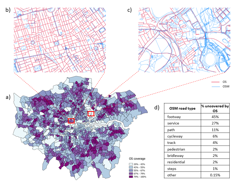
Figure 1: OS and OSM road network coverage in London, UK. a) Percentage of OS over OSM road coverage, based on road linear metres per MSOA level. b) and c) Overlapping of OS and OSM networks showing differences in coverage depending on the urban structure of London areas, Marylebone and Stratford respectively. Table in d) shows the percentage of linear metres from roads on OSM that are not covered by the OS network. Percentages are organised by road types.

The two sources used present some differences that need to be put in context, as evidenced by the comparison in figure 1. Although both data sets could differ in terms of geographical extent, geometrical shape and attribute accuracy of segments, this comparative study focuses mainly on the completeness of the data sets. We examine to what extend their coverage is suited for the analysis of pedestrian and cycling networks. OS Open Roads considers exclusively roads that are used by cars, while OSM represents a wider range. On figure 1 one can see the two data sets overlayed on two areas: in Fitzrovia (b) and Stratford (c). The blue network being OSM and red being OS. In b), most of the roads can be taken by car, the only differences can be seen in pedestrian paths crossing squares and parks. But when looking at the area of Stratford, the differences become more striking. In this case, the OSM network presents a much greater set of roads, which are primarily dedicated to pedestrians and cyclists, including those around and inside the mall and the Olympic park. Further inspection shows that the difference of road linear metres coverage for both networks is unevenly distributed across MSOAs (Figure 1a). Knowing in advance that OS is a more high-level representation of roads, the higher coverage percentage of OSM is not a surprise. However, the high difference between MSOAs is a fact to consider when analysing the results in areas with different urban structures. We then examined whether the difference was consistent across street types, so we measured the percentage that are not covered by the OS dataset. Results show that streets classified as footways, service, paths and cycleways in OSM are under covered by OS (Figure 1d).

2.2 Network setup

This section introduces some of the commonly used open source tools to download and construct a road network. OSM data can be downloaded from a number of sources, including the OpenStreetMap website and dedicated download servers like Geofabrik , which help download raw OSM data in different formats as files with multiple layers of features. Optimal access to this data can be achieved by using many software packages across different programming languages. We mainly consider R and python packages as they are widely used in the community. With each being designed for different purposes, the format and attributes within the data can vary. We considered a non exhaustive list of packages and the main criteria used to select the appropriate one are shown in table 1. OSMnx [4] is a python package,osmdata [37] and osmextract [16] are R packages. We examine and compare different sources for downloading and working with OSM road networks to evaluate which is the most suitable considering the requirements of our analysis (Table 1). Therefore, we will be using OSMnx as the source of OSM data.

	osmdata	osmextract	Geofabrik	OSMnx
Big data	no	yes	yes	yes
Optimal for building graphs	no	no	no	yes
High details	yes	yes	yes	no

Table 1: Overview of packages for working with OSM road networks. This list is non exhaustive and contains the options considered [28, 5, 9] as well as the main criteria for selection. The first category, Big data implies that it is possible to download region and country scale data sets. Optimal for building graphs means that the downloaded data is structured in a way that allows to build graphs without further engineering. Usually, it would be divided into two data sets, one containing nodes with their id, coordinates and additional optional attributes. The other data set contains edge ids, origin node id, destination node id and extra optional arguments such as length. Finally, High details means that several columns of OSM key$\sim$tag values are present additionally to the main classification corresponding to the highway key. Additionally, some even more powerful command line tools are available, and would be useful for a bigger scale of analysis, but are omitted from this work.

As streets have varying attributes and serve distinct purposes, network modelling for specific modes of transportation, such as buses or private cars, only incorporates streets suitable for those modes. However, when it comes to walking and cycling networks, the definition is less precise as pedestrians and cyclists can move more freely throughout the city. This has promoted the interest for creating alternative network profiles using the OSM network as a base. Therefore, additionally to downloading the desired networks, some packages offer the functionality to filter the roads based on a specific mode of transport, like walking, cycling or driving. The OSMnx package in python provides profiles for different transport modes by filtering out streets based on the tag keys. The dodgr [36] package in R creates alternative profiles by weighting the segments according to different attributes such as speed, preferences and restrictions. Moreover, since both profiles rely on the accuracy of the attribute tags given to each street when it is mapped on the OSM network, we first examined whether some of the streets were miss-classified resulting in the inappropriate exclusion or inclusion of street segments (Figure 2).

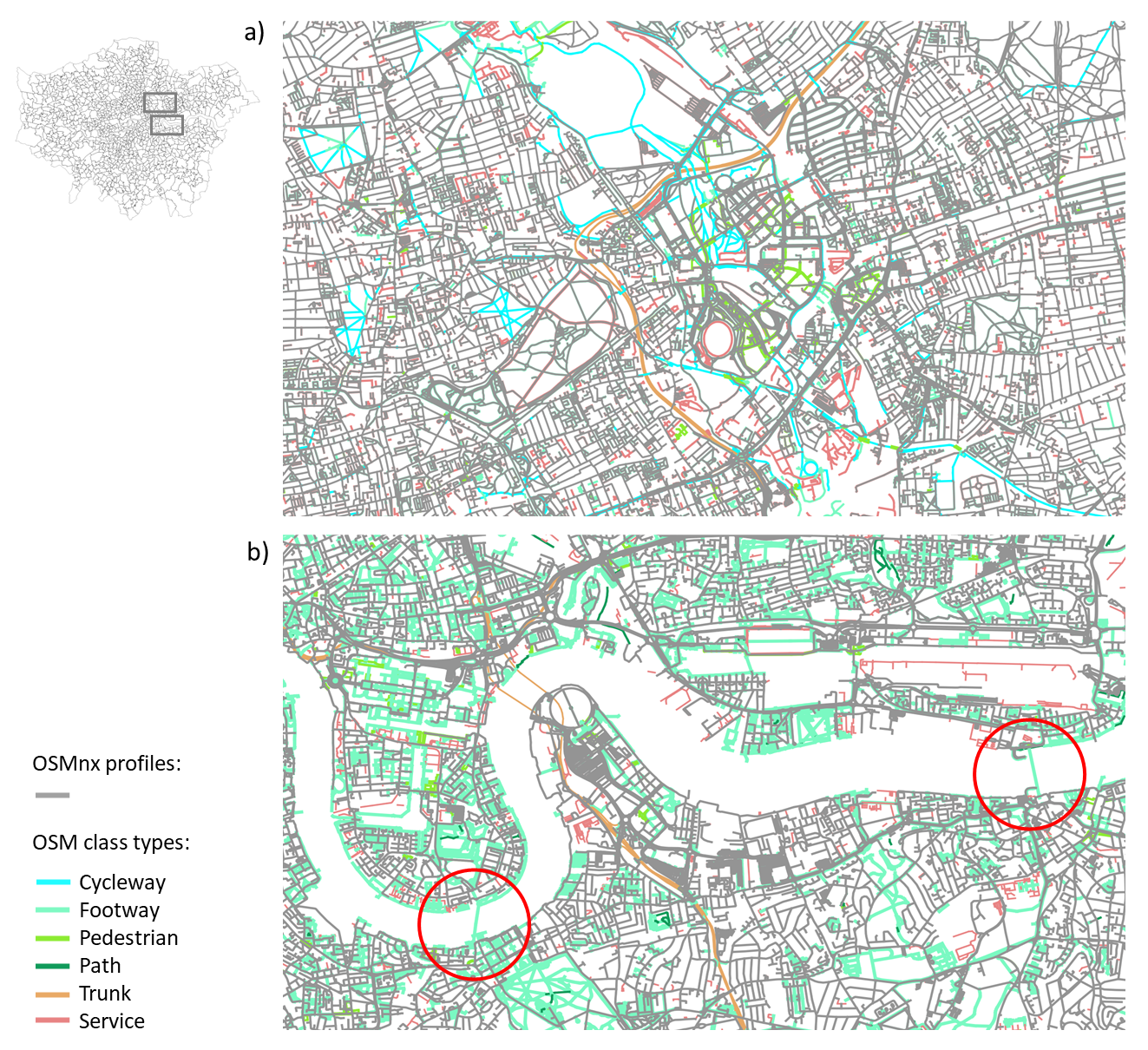
Figure 2: OSMnx walk and cycle profiles overlapping the OSM full network. The OSM full network in different colours showing the class types that are filtered out in the walk and cycle network. a) In grey the OSMnx walk profile on top of the full network. In cian The Greenway footpath running from Victoria park to the southeast, and classified as cycleway. Other footpaths within parks are also classified as cycle ways only. b) In grey the OSMnx cycle profile, in green, the Woolwich and Greenwich foot tunnels highlighted. Given that these tunnels are classified as footways in the OSM network, they are filtered and not considered within the cycle profile.

By looking at figure 2, the streets that were filtered out (in colors) from each profile (in gray) can be identified. For instance, in the case of walking (a), some routes along parks and The Greenway footpath, which runs from Victoria Park to the southeast are excluded from the network as are classified as cycleways in the OSM dataset. A similar case is that of (b), where the tunnels that cross the Thames are excluded from the cycling network as they are classified as footways. As a result, connectivity costs are increased, which may affect global and local patterns, such as the connectivity within East London or between the north and south areas of the river.

Based on these initial observations, different network profiles are used to create distinct OD cost matrices between MSOAs, including those provided by popular packages, and one where minimal filtering was done (motorways removed as forbidden to cycle or walk on) to serve as a base model for our tests. The Ordnance Survey (OS) data is also used as it is the official and open source reference for the road network in the UK.

3 Routing

The next step in developing our analysis consists in using the networks for routing origins and destinations. In the scope of this work, we will only look at the distances that separate OD pairs in the network by using shortest paths algorithms. To accomplish this, we compared a set of commonly used packages for computing shortest paths. We then examined various approaches to determine origin-destination points for commuting, particularly when data is aggregated at geographical units, such as the MSOA level in this case. As a result of this procedure, different cost matrices are created, one for each network, which will serve as inputs for the following section to obtain the prediction of pedestrian and cycling commuting flows.

3.1 Shortest paths

We consider the distance between an origin and destination in a specified network to be the length of the shortest path that connects them. An alternative approach that can be used and is already implemented with certain packages is to consider time. An extra layer of sophistication can also be added by attributing additional weight factors to each link of the network based on its classification and the willingness of cyclists or pedestrians to use it. For example, a commuter might have a tendency to use a smaller, quieter route of greater length rather than a shorter, but busy and risky one. For the purposes of our work, we prioritise distance as the most critical factor for commuting decision-making, which also provides an approach that is easy to implement for a large scale analysis and can be further developed with more variables in future works. The other methods could be useful to learn more about path choice of commuters, who on the one hand think about their safety and comfort, but on the other aim to minimise their trip distance or duration. The significance of other factors may be challenging to validate and is left out of the scope of this work.

Table 2: Mean and median times in seconds to compute a distance matrix between 50 and 100 randomly chosen locations. Different types of heaps are tested for dodgr and two different algorithms for cppRouting, as well as multiple core run when this functionality is provided. sf_networks [53] is a package that, together with tidy_graph [39] relies on igraph [10] for routing. Tests are done with the microbenchmark [31] package in R. The hardware used is a 2022 M2 MacBookPro with 16 GB RAM.

		1 thread, 50x50 OD		4 threads 100x100 OD
package	option	mean	median	mean	median
tidygraph	-	5.13	5.13	-	-
sf_networks	-	4.10	4.06	-	-
dodgr	fheap	24.12	22.92	18.66	17.81
dodgr	bheap	16.87	16.89	13.91	13.90
dodgr	triheap	26.96	26.61	20.54	19.79
cppRouting	phast	2.40	2.41	1.37	1.37
cppRouting	mch	0.35	0.34	0.37	0.37

Based on the outputs from the benchmark shown in table 2, we use the cppRouting package in R to perform the one-to-one and many-to-many calculations and to build distance matrices. This package implements fast, multi-threaded processes, relying on the Dijkstra [49], A-star and PHAST algorithms as well as a contraction hierarchy optimisation which greatly reduces computational times on big graphs.

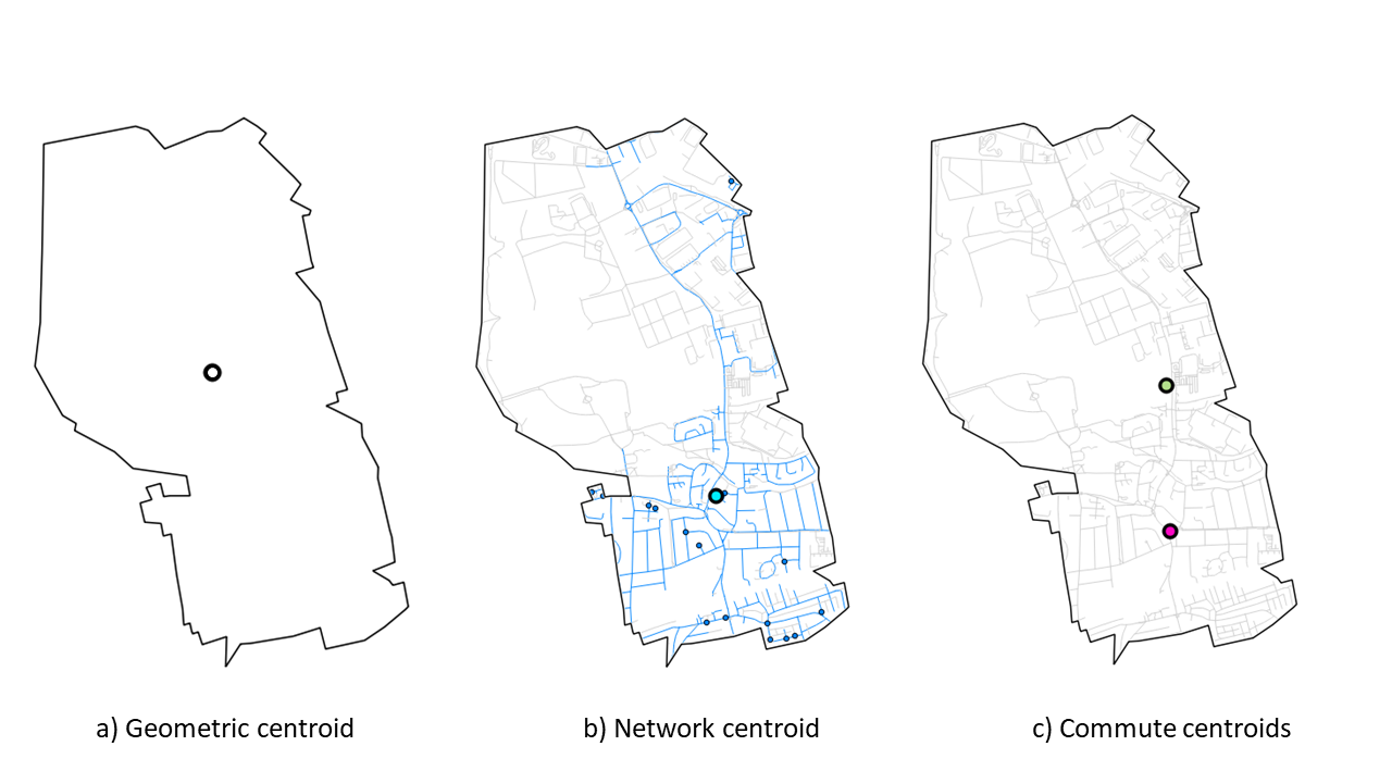
Figure 3: Origin-destination centroids (Beddington MSOA illustrated here). a)The geometric centroids from every MSOA polygon. b) The network centroid based on the distribution of the street network within the MSOA boundary by taking the centre of mass of a sample of road intersections between “living street", “primary", “secondary", “tertiary", “trunk" and “residential" OSM road types (in blue). c) The "commute" centroids, based on the population distribution (origin) in pink and job location (destination) in yellow.

3.2 Selecting origins and destinations

The next aspect of routing consists in solving the what to what problem, namely determining the actual locations to use as the origin and destination. This step is particularly important when the data is aggregated by relatively big units of space (MSOA). For smaller units, like output areas (OA), this question might not be as relevant, because they cover only the area of a few houses, and thus a regular centroid will not bear significant difference from any other node within an area. However, for larger areas that span about $1\unit{km}$ and include multiple streets, overlap parks, rivers and rails, this can become significant, as is demonstrated later on. Although it seems appropriate to choose the smallest available resolution, breaking down the system into small sub units comes at a great cost when running any model. Aiming to develop a methodology that could further on be scaled up to the country level, the MSOAs were used, with 983 in London.

We further consider 3 types of MSOA centroids that are illustrated in figure 3. The first one is the geometric centroid, that is quite commonly used in research [3, 59]. The second one is referred to as network centroid and is the centroid of a sample of nodes that lie within residential roads, this allows to exclude parks, industrial or shopping areas. The third one is a tuple of nodes. The first being the population weighted centroid that accounts for the distribution of residents in space, and the other being the workplace weighted centroid, that is obtained using the definition of workplace zones in the UK statistics office. We refer to this pair as the commute centroids. For each centroid point, the nearest network node is assigned and the distance between them is added to the final matrices.

3.3 Flows data

In the following, the methods and data described earlier will combined with flows data to develop a metric that helps understand the commuting patterns of active travellers.

The commuting data in this work comes from the 2011 UK census and is accessed through the governmental data portal (See details in the appendix). It is available in its raw format for research purposes to individuals linked to a university. The flows contain information on the origin area, destination area, and method of travel, for more details on the variables refer to the online material. Different levels of spatial units are used in the UK census, and this study relies on MSOAs, which are constructed to contain around 8000 individuals each. In this work, only the data for cycling and walking is used for the flows. Additionally, the flows on distances beyond 15km are considered as outliers or collection errors and are excluded.

3.4 Detour index

When measuring the performance of networks in terms of distance, as in the context of transport studies, it is useful to look at a measure called the detour index, also referred to as circuity [2], which can take different forms if we consider a whole network or a node, or a specific route:

$$\delta_{ij,k}=\frac{l_{ij,k}}{d_{ij}}$$ (1)

where $l_{ij,k}$ is the distance in the network $k$ between location $i$ and $j$, and $d_{ij}$ is the Euclidean distance between them. If aggregating on an origin node and considering a set of destination nodes, which is not necessarily all the nodes in the network:

$$\delta_{i,k}=\frac{1}{N_{S}-1}\sum_{j\in S,i\neq j}\delta_{ij,k}$$ (2)

which gives the average detour index of the routes from node $i$ to all other nodes of interest in set $S$ for a specified network $k$. And, for the whole network other the set of nodes $S$:

$$\delta_{k}=\frac{1}{N_{S}(N_{S}-1)}\sum_{ij\in S,,i\neq j}\delta_{ij,k}$$ (3)

where $N_{S}$ is the number of nodes in set $S$. The detour index is greater or equal to 1, and the more efficient, or straight, a network path is the closer the value will be to 1. Typical values are between $1.1$ and $1.5$ and values over 2 show a poor performance [24, 58]. This index has been linked to important aspects of the network such as accessibility and efficiency. In [9], the detour index was found to decrease with time in cycling networks. This indicates a tendency of the network to ameliorate it’s connectivity, by growing new links or changing the routing possibilities. In [24] it was observed that users of the network tend to locate in places that minimise detour for their commuting trip compared to a random selection of origin-destination pairs. The authors observe different values of average detour for random selections of OD nodes compared to observed OD flows, indicating that the efficiency of the network is better understood through the mobility patterns occurring in it. Hence, the consideration of a subset $S$ of the nodes involved in observed OD flows, in our case the MSOA with flows between them, is relevant to better understand commuting trip distributions in the network.

In this section we took the different street networks and consider the geometric centroids as origin-destination points for a straightforward comparison.

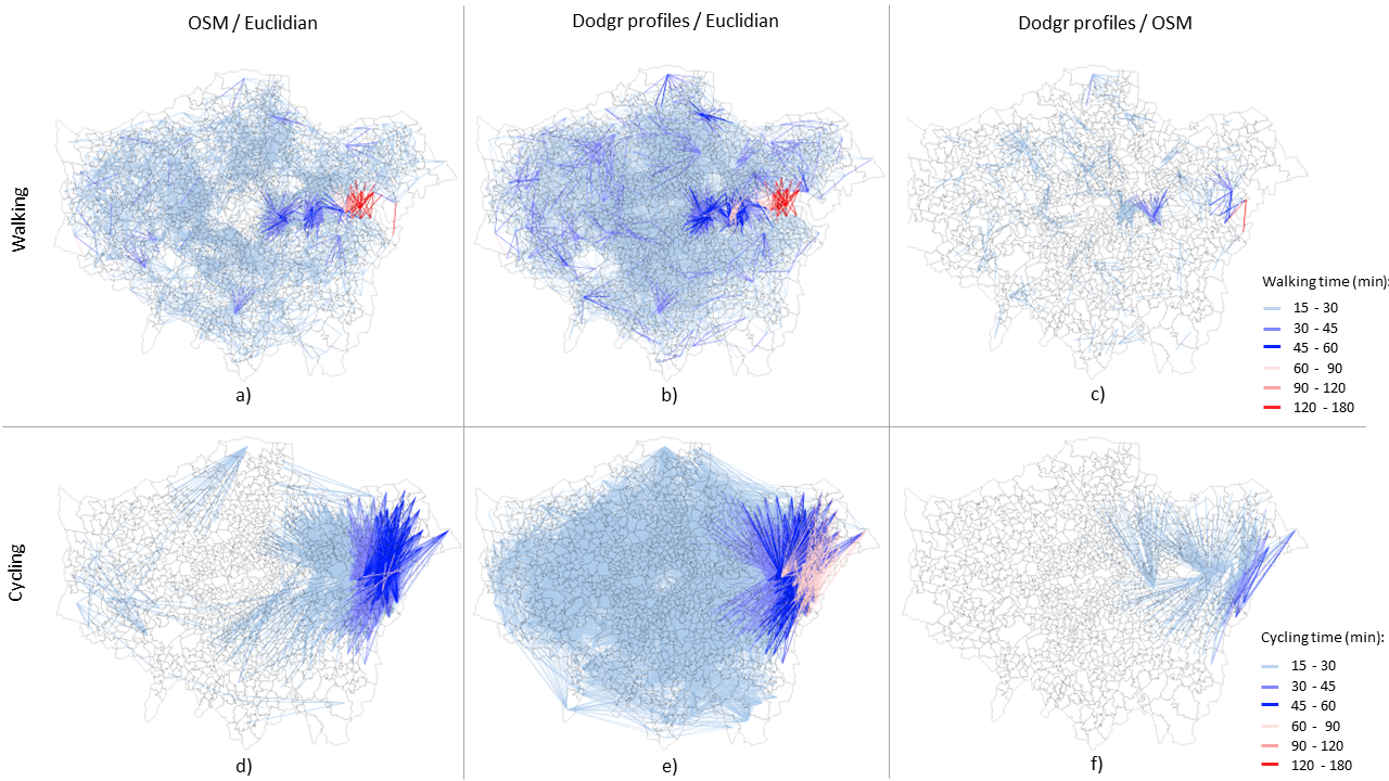
Figure 4: Detour given walking and cycling times when comparing shortest paths from the OSM and dodgr networks with the euclidian distances between MSOAs. We converted distance into time cost using 1.3 m/s and 4.2 m/s as the walking and cycling speeds, respectively. We excluded trips wich would take longer than 1 hour as a maximum threshold for commuting by these modes. We visualised differences in time longer than 15 minutes as a way to highlight detours that would have a greater impact on the decision to use active travel

We plot the detour distance values in Figure 4, translated into walking and cycling times, to make the comparison of both modes easier. Differences in the cost of the shortest paths between MSOAs are considerable across space. Results are highly determined by the uneven distribution of the street network provision and network impedance. Due to the lack of crossings in the east, for example, MSOAs at each side of the Thames present the higher detour values with commuting times reaching a difference of up to 3 hours. Higher differences can be found in MSOAs with large green areas, large block sizes and other barriers like train lines. Based on the results, when comparing the different commuting times it is important to consider that the differences between the network distances are not evenly distributed in space, and that the selection of one or the other may affect the results of future analyses in specific areas of the city.

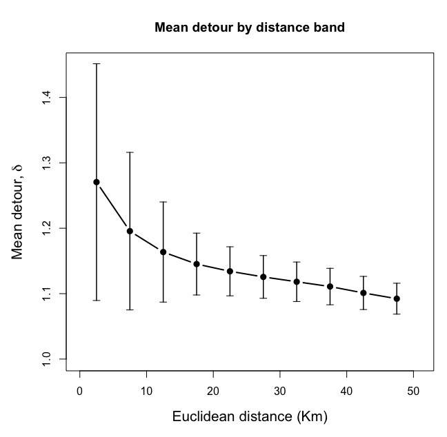
(a)

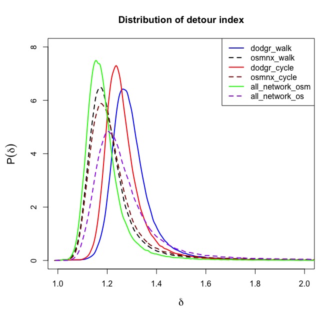
(b)

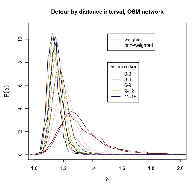
(c)

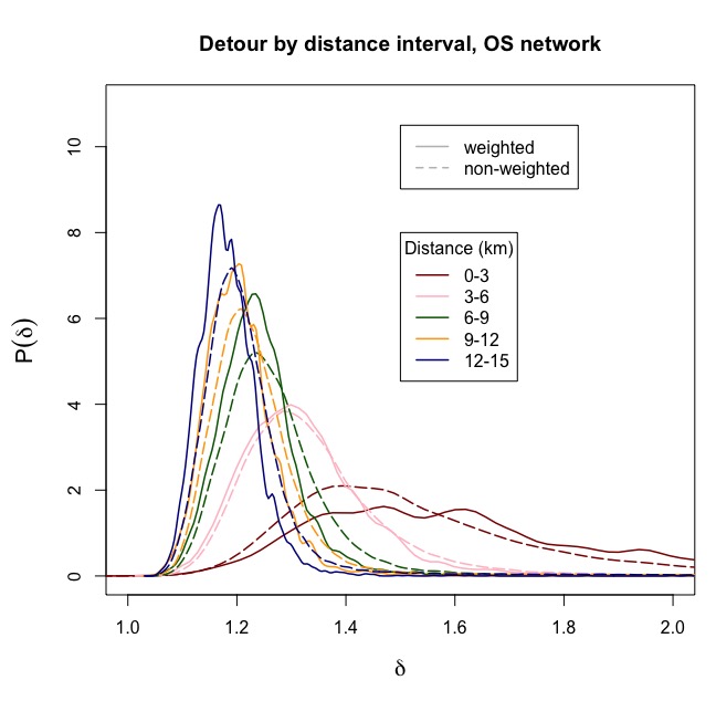
(d)

Figure 5: The detour index is the ratio of the distance between two points in the network chosen and the shortest, Euclidean distance, $\delta^{k}_{ij}=\frac{l_{ij,k}}{d_{ij}}$, where $l_{ij,k}$ is the distance in the network $k$, and $d_{ij}$ is the Euclidean distance between those points. Clearly, $\delta\in[1,\infty[$. One can see that the kind of routing (fig 5(b)) proposed by the $\boldsymbol{dodgr}$ package results in longer shortest paths due to the weighting that favours smaller roads to bigger, busier ones for cyclists and pedestrians. The network that approaches the most the theoretical case of $\frac{\sum_{i,j=1}^{N}\delta^{k}_{ij}}{N(N-1)}=\bar{\delta^{k}}$ = 1, is the OSM full network, which contains short cuts and links not included elsewhere. The Ordnance Survey network (dashed purple line) is the least efficient of the networks without custom weighting profiles. On 5(a), one can observe the decreasing average detour and shrinking standard deviation as the Euclidean distance between locations increases. On figures 5(c) and 5(d), the detour distribution, weighted (solid line) and non weighted (dashed line) by commuter flow for different distance intervals of Euclidean distance of trips. The table in the appendix, presents the same observation for finer distance intervals, removing the effects of the growing number of destinations with distance.

d (km)		OS			OSM
min	max	$\delta_{c}$	$\delta_{n}$	t-test	$\delta_{c}$	$\delta_{n}$	t-test
0.0	0.6	2.113	2.108	0.1	1.498	1.518	-0.8
0.6	0.9	1.931	1.914	0.9	1.454	1.471	-1.6
0.9	1.2	1.780	1.791	-0.7	1.384	1.423	-4.9
1.2	1.5	1.666	1.700	-3.0	1.357	1.388	-4.7
1.5	1.8	1.610	1.623	-1.4	1.307	1.347	-8.5
1.8	2.1	1.538	1.535	0.5	1.266	1.313	-14.0
2.1	2.4	1.464	1.514	-7.4	1.253	1.303	-15.2
2.4	2.7	1.454	1.473	-3.5	1.237	1.284	-16.6
2.7	3.0	1.402	1.457	-9.5	1.232	1.274	-14.8

Table 3: This table summarises the detour for commuting trips and for typical network values by distance ranges between origin and destination. It shows how they significantly differentiate, especially as crow fly distance grows (column $d$). In this table, we look at granular intervals, within the distance band 0-3km (darkred distributions from figures 5(c) and 5(d)), the full table for up to 15km is given in the appendix.

The distribution of all $\delta_{ij,k}$ is shown in figure 5(b). It is not surprising to see that the resulting $\boldsymbol{dodgr}$ networks with a custom weighting profile, which tends to increase the actual distances, show greater values. The results for the remaining networks are more similar, with slightly increasing mean and variance from the whole OSM network, followed by the OSMnx walk and cycle profiles and finally OS. To our knowledge, there is no research linking typical detour values to the density of the nodes and edges of the network, however, it seems intuitively natural for a detour to increase as a consequence of removing edges from a network. Hence, sparser networks are expected to have greater typical detour values.

We further develop the detour index to account for the flows observed across a set of origin-destination pairs. Let $w_{ij}$ be a flow observed between origin $i$ and destination $j$, by weighting the detour values with the flow, we obtain a more accurate representation of the detours that commuters take on average during their commute:

$$\delta_{c}=\frac{1}{W}\sum_{i,j\in S,i\neq j}w_{ij}\delta_{ij,k}$$ (4)

where $W=\sum_{i,j\in S,i\neq j}w_{ij}$ is the total flow between different origins and destinations.

One of the main characteristics of flows is that their magnitude decreases as we get further from an origin. They also show a wider range of values for shorter distances, spanning several orders of magnitude. At the same time, we observe a decreasing average detour index as the Euclidean distance increases (fig. 5(a)) between origin and destination, while the potential number of reachable destinations from an origin grows approximately as the square of the distance. These different trends introduce some non trivial relations between flows, their magnitude, the distances on which they occur and their detour values. To further uncover some patterns relating these, we look at the distribution of the mean weighted detour (equation 4) of a trip and the mean detour of the network in 300 metres intervals of Euclidean distance between 0 and 15 km. In this way we minimise the effects of a varying Euclidean distance, and focus only on the typical values of the detour weighted and non weighted by flow. Within each resulting interval we test for the significance in the difference between the means, and find that it becomes strong (p-value $\approx 0$) inside the interval 900-1200 metres (see table 3) and remains statistically significant for all the distances beyond that. Moreover, the t-statistic gets stronger as the Euclidean distance increases. This indicates that for shorter trips, detour has a less significant or no impact on the trip, but as the distance increases, we observe a significant shift of the average weighted detour towards smaller values. This observation can be useful when designing road infrastructure, where aiming to minimise a weighted detour index of a population can potentially have a positive effect on the number of trips done between locations, especially as the Euclidean distance separating points gets greater. Figure 5(a) shows an example distribution of detours with wider intervals for better visualisation purposes. We observe that as the Euclidean distances increase, the distribution of detours narrows down and shifts towards a smaller mean. This behaviour seems to be a fundamental property of the detour index and has been observed for other real world road networks. The full results for granular distance intervals and statistical significance is included in the appendix table 4.

4 Modelling

This section considers the previous results and integrates the distance matrices produced from the different network profiles and origin-destination centroids into a spatial interaction model. With the available flows data, a doubly constrained gravity model is built and tested.

4.1 Spatial interaction models

This family of models, also referred to as gravity models, has been around for a while and was formalised in the late 1960s by [55]. It allows to build good predictions of flows based on input variables that are relatively easy to find. The name originates from the similarity with the gravity law derived by Isaac Newton. This problem has been reformulated and formalised with statistical considerations of the optimal assignment from a set of origins in a grid to a set of available destinations under a cost value that depends on the distance. Intuitively, we consider that there are factors contributing to a greater flow of people between 2 given places and others reducing it. Some parameters will thus be directly proportional to the flow of people while others will be inversely so. The factors contributing to the flow positively are usually taken to be the population at the origin location and the job availability at the destination, while the distance between the two locations has a inverse effect on the flow. Formally, this means that $T_{ij}\sim O_{i}D_{j}f(d_{ij})$ where $O_{i}$ is the origin population in location $i$, $D_{j}$ is the employment at the destination location $j$, $f(d_{ij})$ is a decreasing function of the distance, usually referred to as generalised cost. The known constraints of the system impose that all the flows originating at a location $i$ must be equal to the local working population, while all the flows arriving to a destination $j$ be equal to the local number of jobs, thus:

$$\begin{split}O_{i}=\sum_{j}T_{ij},\\ D_{j}=\sum_{i}T_{ij}\end{split}$$ (5)

The travel cost function can be derived [55] and has the form $f(d_{ij})=e^{-\beta d_{ij}}$, where $\beta$ is an exponent that depends on the system and is usually calculated for different modes of transport and geographies. Additionally, the origin and destination weighting parameters are obtained through the Lagrange multipliers method, resulting in a equation of the form:

$$T_{ij}=A_{i}O_{i}B_{j}D_{j}e^{-\beta d_{ij}}$$ (6)

which is referred to as the doubly constrained one since the available information about the system allows to set constraints on both the origin and destination locations. Alternatively, if some information is missing, it is possible to use only one constraint.

The parameters $A_{i},B_{j}$ are derived from the expression:

$$\begin{split}A_{i}=[\sum_{j}B_{j}D_{j}e^{-\beta d_{ij}}]^{-1}\\ B_{j}=[\sum_{i}A_{i}O_{i}e^{-\beta d_{ij}}]^{-1}\end{split}$$ (7)

with values obtained through an iterative process [11].

The flows data is obtained via the census table with origin destination pairs and number of commuters by mode of transport. The distance measures can be obtained in different manners as discussed in section 3. The distance matrices obtained are used in the gravity model further on.

4.2 Case Study: active travel commuters in London.

The methods described in the first two sections will now be combined with the formalism of spatial interaction models to have a predictive model of active travel commuter flows in London based on the different networks and centroid types that were introduced.

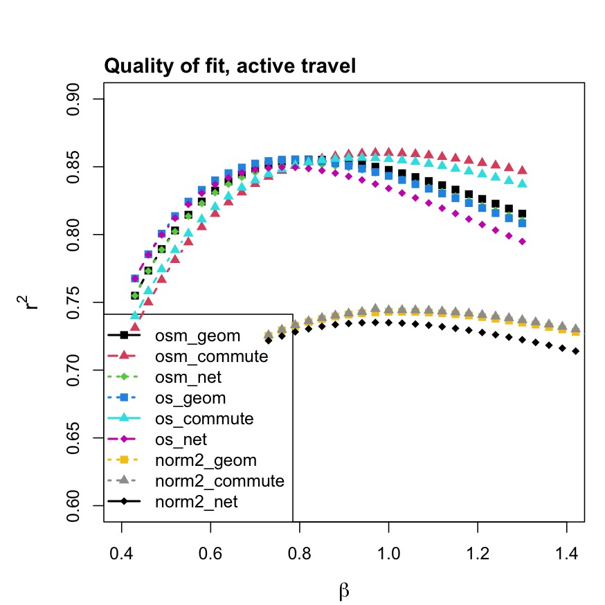
(a)

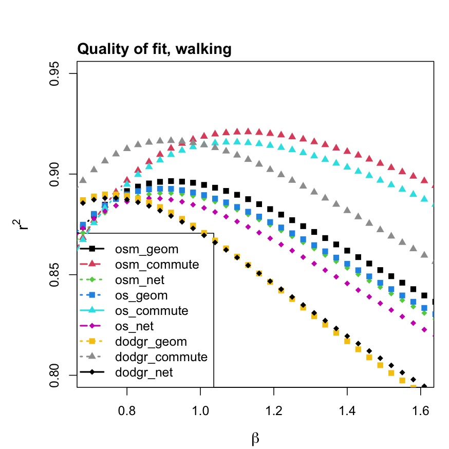
(b)

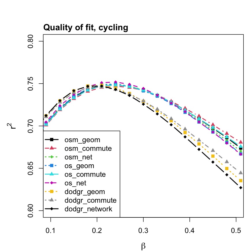
(c)

Figure 6: Quality of fit calibration for different networks, mode, centroids. The most significant impact on the quality of fit occurs when changing centroids on the pedestrian model. Each legend element has first mentioned the network from which the cost matrix (os,osm,dodgr,norm2), with norm2 indicating the crow-fly distances matrix. And as second the type of centroids used.

The methods and data described earlier allows for a generalised approach to modelling flows, and when applied to active travel commuters, provide some high quality of fit results in the case study of London. Figure 6(a) shows the results of the calibration of the model to maximise the $r^{2}$ value. The quality of fit of the models using Euclidean distance between locations as cost is also computed and, despite being lower than network distance, provides a good estimate of the flow with values reaching $r^{2}=0.75$. One can see that depending on the network, the maximum is reached for differing values, and certain types of networks provide a better stability of the quality of fit under a varying $\beta$ exponent than others. While all the networks reach a high and very similar value of around $r^{2}=0.85$, they do it for different values and the best quality of fit is reached with the OSM and OS networks using commute centroids, indicating the importance of the discussion in section 3.2 on the knowledge of where the routing is being done. The network and geometric centroids appear less adapted for routing based on the quality of fit obtained for all types of network considered.

5 Discussion and conclusion

In this work, we first conducted a methodological analysis covering network, routing and modelling steps. By comparing different walking and cycling networks and prioritising distance as a critical factor in commuting route choice for active travel, we explored their capacity to estimate real-world flows using a spatial interaction model. We use London as case study, using the 2011 census flows at MSOA level. Throughout the process, we observe that the use of different data sources, network construction, and routing approaches can lead to diverse outcomes in the analysis, both at a broad city-wide scale and at a more local level in different areas of the city. We illustrate the limitations of the OSM data when attempting to select network profiles for specific modes of transport. To counter these limitations, we keep a network that is filtered only to exclude the types of roads that are illegal to use as an active traveller, those are motorway and motorway links and propose a combined active-travel framework allowing to model cycling and walking trips. The results of the spatial interaction model show that this type of network performs best when associated to what we defined as commute centroids, accounting for the spatial distribution of residents and jobs inside the census areas. The spatial interaction model that we calibrated on this combination of network and centroid was the best fitting and most stable across the cost function exponent values, highlighting the importance not only of the parameters related to the network itself, but also to the routing process. The quality of fit values for all networks were relatively high, and the best predictions were obtained using the unfiltered OSM and OS networks with commute centroids.

We further investigate the commuting trip patterns by using the detour index. It shows to be a useful measure for assessing the performance of different networks at minimising the trip length for a given Euclidean distance. We introduce the weighted detour index and show the tendency of London’s active travellers to commute in a way that minimises the detour of their trip when the Euclidean distance to their job is beyond 900-1200 metres. Minimising the detour on the way to work seems to be important to active travel commuting, especially as the Euclidean distance between origin and destination increases. We also observe considerable spatial variation in the potential walking and commuting time between MSOAs, which is determined by the uneven distribution and connectivity of the network, as well as the inconsistencies in data sources, which can impact the models that are built on top of them. These findings emphasise the importance of careful consideration and validation of the input data coming from any kind of sources, whether official or crowd sourced. The network with the lowest average detour index also showed the best fitting in the spatial interaction model. This indicates the possibility to use this index as a guide when designing new infrastructure that aims to connect a population to an employment distribution in a way that minimises the weighted detour of the trips. The main focus of this work is done on active travel as a mean to commute, but the applications and possibilities of the models and methods go beyond that and provide a general framework on open source data for active-travel modelling. Our research has implications for urban planning and policy-making, as it highlights the need for accurate network data and appropriate modelling techniques to inform the development of sustainable transport infrastructure and promote active travel in cities.

6 Acknowledgements

This paper has received funding from the QUANT and RUBICON projects from the Alan Turing Institute under grant TU/ASG/R-SPEU-102.

7 Appendix

7.1 Online material and reproducibility

The main code and process to access the data are described here. Limitations due to the accessibility of the census flow forbid us to provide it here, but an institutional account allows to connect and download the detailed msoa level flows data from the WICID portal via an account created on UKDataServices .

Code: https://github.com/ischlo/quant_cycle_walk

Additionally, a mini package called cppSim was developed to perform fast and memory efficient spatial interaction models, it is made available in the following github repository: https://github.com/ischlo/cppSim

d (km)		OS			OSM
min	max	$\delta_{c}$	$\delta_{n}$	t-test	$\delta_{c}$	$\delta_{n}$	t-test
0.0	0.6	2.113	2.108	0.1	1.498	1.518	-0.8
0.6	0.9	1.931	1.914	0.9	1.454	1.471	-1.6
0.9	1.2	1.780	1.791	-0.7	1.384	1.423	-4.9
1.2	1.5	1.666	1.700	-3.0	1.357	1.388	-4.7
1.5	1.8	1.610	1.623	-1.4	1.307	1.347	-8.5
1.8	2.1	1.538	1.535	0.5	1.266	1.313	-14.0
2.1	2.4	1.464	1.514	-7.4	1.253	1.303	-15.2
2.4	2.7	1.454	1.473	-3.5	1.237	1.284	-16.6
2.7	3.0	1.402	1.457	-9.5	1.232	1.274	-14.8
3.0	3.3	1.377	1.430	-10.8	1.226	1.265	-11.6
3.3	3.6	1.368	1.409	-9.3	1.213	1.250	-17.3
3.6	3.9	1.343	1.393	-12.0	1.204	1.248	-19.2
3.9	4.2	1.329	1.384	-12.6	1.195	1.242	-18.5
4.2	4.5	1.319	1.372	-13.4	1.191	1.237	-19.7
4.5	4.8	1.301	1.361	-15.1	1.184	1.229	-21.0
4.8	5.1	1.293	1.356	-16.7	1.182	1.228	-19.8
5.1	5.4	1.285	1.344	-16.7	1.177	1.222	-24.2
5.4	5.7	1.279	1.334	-17.3	1.171	1.218	-24.2
5.7	6.0	1.267	1.327	-19.2	1.168	1.212	-26.4
6.0	6.3	1.259	1.323	-21.4	1.164	1.211	-28.8
6.3	6.6	1.254	1.317	-21.7	1.160	1.208	-28.9
6.6	6.9	1.251	1.307	-21.5	1.155	1.201	-33.2
6.9	7.2	1.240	1.301	-24.5	1.154	1.201	-32.5
7.2	7.5	1.233	1.298	-26.8	1.147	1.198	-38.0
7.5	7.8	1.236	1.293	-23.1	1.155	1.195	-29.2
7.8	8.1	1.232	1.285	-24.3	1.149	1.192	-36.9
8.1	8.4	1.223	1.280	-27.2	1.142	1.189	-37.2
8.4	8.7	1.225	1.278	-24.6	1.145	1.187	-36.8
8.7	9.0	1.221	1.273	-25.7	1.143	1.184	-36.8
9.0	9.3	1.216	1.268	-26.3	1.145	1.182	-33.3
9.3	9.6	1.211	1.264	-29.8	1.135	1.179	-47.3
9.6	9.9	1.206	1.261	-30.0	1.137	1.179	-40.4
9.9	10.2	1.209	1.255	-26.7	1.141	1.177	-36.2
10.2	10.5	1.206	1.254	-29.1	1.139	1.175	-38.4
10.5	10.8	1.201	1.249	-30.7	1.134	1.173	-40.6
10.8	11.1	1.201	1.244	-29.0	1.135	1.171	-40.0
11.1	11.4	1.195	1.242	-31.8	1.134	1.169	-39.7
11.4	11.7	1.199	1.240	-28.9	1.139	1.168	-31.4
11.7	12.0	1.197	1.239	-29.3	1.137	1.168	-35.9
12.0	12.3	1.189	1.232	-28.9	1.132	1.164	-35.3
12.3	12.6	1.187	1.230	-34.7	1.130	1.163	-43.0
12.6	12.9	1.192	1.228	-28.1	1.133	1.162	-37.7
12.9	13.2	1.185	1.226	-32.1	1.133	1.161	-35.4
13.2	13.5	1.184	1.224	-34.3	1.127	1.160	-48.8
13.5	13.8	1.183	1.220	-32.7	1.132	1.158	-38.5
13.8	14.1	1.185	1.217	-28.6	1.133	1.157	-34.6
14.1	14.4	1.179	1.216	-35.4	1.123	1.156	-52.8
14.4	14.7	1.181	1.213	-31.1	1.127	1.154	-43.5
14.7	15.0	1.180	1.210	-31.4	1.130	1.153	-39.2

Table 4: This table summarises the detour for commuting trips ($\delta_{c}$) and for typical network values ($\delta_{n}$) within distance ranges of crow-fly distance. It shows how they significantly differentiate, especially as crow fly distance grows (column $d$). We test the significance in the difference of the observed means for the weighted detour compared with regular network values. The results show that the observed difference are strongly significant, especially as the crow fly distance between locations increases.

References

- [1] Marc Barthelemy “From paths to blocks: New measures for street patterns” In Environment and Planning B: Urban Analytics and City Science 44.2, 2017, pp. 256–271 DOI: 10.1177/0265813515599982
- [2] Marc Barthélemy “Spatial networks” In Physics Reports 499.1, 2011, pp. 1–101 DOI: 10.1016/j.physrep.2010.11.002
- [3] Aleix Bassolas et al. “Hierarchical organization of urban mobility and its connection with city livability” In Nature Communications 10.1, 2019, pp. 4817 DOI: 10.1038/s41467-019-12809-y
- [4] Geoff Boeing “OSMnx: New methods for acquiring, constructing, analyzing, and visualizing complex street networks” In Computers, Environment and Urban Systems 65, 2017, pp. 126–139 DOI: 10.1016/j.compenvurbsys.2017.05.004
- [5] Geoff Boeing “The Morphology and Circuity of Walkable and Drivable Street Networks”, 2018 DOI: 10.31235/osf.io/edj2s
- [6] Geoff Boeing “Street Network Models and Indicators for Every Urban Area in the World” In Geographical Analysis, 2021, pp. gean.12281 DOI: 10.1111/gean.12281
- [7] Joseph Broach, John Gliebe and Jennifer Dill “Bicycle route choice model developed using revealed preference GPS data” In TRB 2011 Annual Meeting 5464, 2011 URL: ftp://ftp.hsrc.unc.edu/pub/TRB2011/data/papers/11-3901.pdf
- [8] Robert Cervero, Steve Denman and Ying Jin “Network design, built and natural environments, and bicycle commuting: Evidence from British cities and towns” In Transport Policy 74.September 2018 Elsevier Ltd, 2019, pp. 153–164 DOI: 10.1016/j.tranpol.2018.09.007
- [9] Miguel Costa, Manuel Marques and Filipe Moura “A Circuity Temporal Analysis of Urban Street Networks Using Open Data: A Lisbon Case Study” In ISPRS International Journal of Geo-Information 10.7, 2021, pp. 453 DOI: 10.3390/ijgi10070453
- [10] Gabor Csardi and Tamas Nepusz “The igraph software package for complex network research” In InterJournal Complex Systems, 2006, pp. 1695 URL: https://igraph.org
- [11] W. Deming and Frederick F. Stephan “On a Least Squares Adjustment of a Sampled Frequency Table When the Expected Marginal Totals are Known” In The Annals of Mathematical Statistics 11.4, 1940, pp. 427–444 DOI: 10.1214/aoms/1177731829
- [12] Jennifer Dill and Theresa Carr “Bicycle Commuting and Facilities in Major U.S. Cities: If You Build Them, Commuters Will Use Them” In Transportation Research Record: Journal of the Transportation Research Board 1828.1, 2003, pp. 116–123 DOI: 10.3141/1828-14
- [13] Vanessa Fleury et al. “Geospatial analysis of individual-based Parkinson’s disease data supports a link with air pollution: A case-control study” In Parkinsonism & Related Disorders 83, 2021, pp. 41–48 DOI: 10.1016/j.parkreldis.2020.12.013
- [14] Susana Freiria, Alexandre O Tavares and Rui Pedro Julião “The multiscale importance of road segments in a network disruption scenario: A risk-based approach” In Risk analysis 35.3 Wiley Online Library, 2015, pp. 484–500
- [15] Riccardo Gallotti, Giulia Bertagnolli and Manlio De Domenico “Unraveling the hidden organisation of urban systems and their mobility flows” In EPJ Data Science 10.1, 2021, pp. 3 DOI: 10.1140/epjds/s13688-020-00258-3
- [16] Andrea Gilardi and Robin Lovelace “osmextract: Download and Import Open Street Map Data Extracts” https://docs.ropensci.org/osmextract/, https://github.com/ropensci/osmextract, 2022
- [17] M Hamer and Y Chida “Walking and primary prevention: a meta-analysis of prospective cohort studies” In British Journal of Sports Medicine 42.4 British Association of SportExcercise Medicine, 2008, pp. 238–243 DOI: 10.1136/bjsm.2007.039974
- [18] César A Hidalgo “Trillion dollar streets” In Environment and Planning B: Urban Analytics and City Science 47.7, 2020, pp. 1133–1135 DOI: 10.1177/2399808320949295
- [19] Bill Hillier, Tao Yang and Alasdair Turner “Normalising least angle choice in Depthmap-and how it opens up new perspectives on the global and local analysis of city space” In Journal of Space syntax 3.2 University College London, 2012, pp. 155–193
- [20] Woo-Sung Jung, Fengzhong Wang and H. Stanley “Gravity model in the Korean highway” In EPL (Europhysics Letters) 81.4, 2008, pp. 48005 DOI: 10.1209/0295-5075/81/48005
- [21] Paul Kelly et al. “Systematic review and meta-analysis of reduction in all-cause mortality from walking and cycling and shape of dose response relationship” In International Journal of Behavioral Nutrition and Physical Activity 11.1, 2014 DOI: 10.1186/s12966-014-0132-x
- [22] Kevin J. Krizek, Susan L. Handy and Ann Forsyth “Explaining changes in walking and bicycling behavior: Challenges for transportation research” In Environment and Planning B: Planning and Design 36.4, 2009, pp. 725–740 DOI: 10.1068/b34023
- [23] Stephen Law, Kayvan Karimi, Alan Penn and Alain Chiaradia “Measuring the influence of spatial configuration on the housing market in metropolitan London” In Proceedings of the 2013 International Space Syntax Symposium, Seoul, Korea 31, 2013
- [24] David Levinson and Ahmed El-Geneidy “The minimum circuity frontier and the journey to work” In Regional Science and Urban Economics 39.6, 2009, pp. 732–738 DOI: 10.1016/j.regsciurbeco.2009.07.003
- [25] Shiqin Liu et al. “A Generalized Framework for Measuring Pedestrian Accessibility around the World Using Open Data” In Geographical Analysis, 2021, pp. gean.12290 DOI: 10.1111/gean.12290
- [26] Rémi Louf and Marc Barthelemy “A typology of street patterns” In Journal of The Royal Society Interface 11.101, 2014, pp. 20140924 DOI: 10.1098/rsif.2014.0924
- [27] Robin Lovelace et al. “The Propensity to Cycle Tool: An open source online system for sustainable transport planning” In Journal of Transport and Land Use 10.1, 2017 DOI: 10.5198/jtlu.2016.862
- [28] Hussein Mahfouz, Elsa Arcaute and Robin Lovelace “A Road Segment Prioritization Approach for Cycling Infrastructure”, 2021, pp. 1–31 arXiv: http://arxiv.org/abs/2105.03712
- [29] Stephen Marshall et al. “Street network studies: from networks to models and their representations” In Networks and Spatial Economics Springer, 2018, pp. 1–15
- [30] A. Masucci, Kiril Stanilov and Michael Batty “Exploring the evolution of London’s street network in the information space: A dual approach” Number: 1 In Physical Review E 89.1, 2014, pp. 012805 DOI: 10.1103/PhysRevE.89.012805
- [31] Olaf Mersmann “microbenchmark: Accurate Timing Functions” R package version 1.4.10, 2023 URL: https://CRAN.R-project.org/package=microbenchmark
- [32] Carlos Molinero, Elsa Arcaute, Duncan Smith and Michael Batty “The fractured nature of British politics” In arXiv preprint arXiv:1505.00217, 2015
- [33] David C Novak and James L Sullivan “A link-focused methodology for evaluating accessibility to emergency services” In Decision Support Systems 57 Elsevier, 2014, pp. 309–319
- [34] P. Oja et al. “Health benefits of cycling: A systematic review” In Scandinavian Journal of Medicine and Science in Sports 21.4, 2011, pp. 496–509 DOI: 10.1111/j.1600-0838.2011.01299.x
- [35] ONS “2011 Census aggegate data (Data downloaded: 1 February 2017)” UK Data Service. Office for National Statistics, 2017 DOI: 10.5257/CENSUS/AGGREGATE-2011-2
- [36] Mark Padgham “dodgr: An R package for network flow aggregation” In Transport Findings Network Design Lab, 2019 DOI: 10.32866/6945
- [37] Mark Padgham, Bob Rudis, Robin Lovelace and Maëlle Salmon “osmdata” In The Journal of Open Source Software 2.14 The Open Journal, 2017 DOI: 10.21105/joss.00305
- [38] Nicolas Palominos and Duncan A Smith “Examining the geometry of streets through accessibility: new insights from streetspace allocation analysis” In Environment and Planning B: Urban Analytics and City Science, 2022, pp. 239980832211398 DOI: 10.1177/23998083221139849
- [39] Thomas Lin Pedersen “tidygraph: A Tidy API for Graph Manipulation” R package version 1.2.1, 2022 URL: https://CRAN.R-project.org/package=tidygraph
- [40] Alan Penn “Space syntax and spatial cognition: Or why the axial line?” In Environment and Behavior 35.1, 2003, pp. 30–65 DOI: 10.1177/0013916502238864
- [41] Duccio Piovani, Carlos Molinero and Alan Wilson “Urban retail location: Insights from percolation theory and spatial interaction modeling” In PLoS ONE 12.10, 2017 DOI: 10.1371/journal.pone.0185787
- [42] Sergio Porta, Paolo Crucitti and Vito Latora “The network analysis of urban streets: a primal approach” In Environment and Planning B: planning and design 33.5 SAGE Publications Sage UK: London, England, 2006, pp. 705–725
- [43] Sergio Porta et al. “Street centrality and the location of economic activities in Barcelona” In Urban Studies 49.7 SAGE Publications Sage UK: London, England, 2012, pp. 1471–1488
- [44] Sergio Porta et al. “Street centrality and densities of retail and services in Bologna, Italy” In Environment and Planning B: Planning and design 36.3 SAGE Publications Sage UK: London, England, 2009, pp. 450–465
- [45] Daniel Rhoads, Albert Solé-Ribalta, Marta C. González and Javier Borge-Holthoefer “Planning for sustainable Open Streets in pandemic cities”, 2020 arXiv: http://arxiv.org/abs/2009.12548
- [46] Gustavo Romanillos, Borja Moya-Gómez, Martin Zaltz-Austwick and Patxi J. Lamíquiz-Daudén “The pulse of the cycling city: visualising Madrid bike share system GPS routes and cycling flow” In Journal of Maps 14.1, 2018, pp. 34–43 DOI: 10.1080/17445647.2018.1438932
- [47] Lucinda E. Saunders et al. “What Are the Health Benefits of Active Travel? A Systematic Review of Trials and Cohort Studies” In PLoS ONE 8.8, 2013 DOI: 10.1371/journal.pone.0069912
- [48] Jessica Schoner and Xinyu Cao “Walking for purpose and pleasure influences of light rail, built environment, and residential self-selection on pedestrian travel” In Transportation Research Record 2464, 2014, pp. 67–76 DOI: 10.3141/2464-09
- [49] Clifford Stein, Charles E Leiserson, Thomas H Cormen and Ronald L Rivest “Introduction to algorithms”, The MIT Press The MIT Press, 2009
- [50] Emanuele Strano et al. “Elementary processes governing the evolution of road networks” Number: 1 In Scientific Reports 2.1, 2012, pp. 296 DOI: 10.1038/srep00296
- [51] Emanuele Strano et al. “Urban street networks, a comparative analysis of ten European cities” In Environment and Planning B: Planning and Design 40.6 SAGE Publications Sage UK: London, England, 2013, pp. 1071–1086
- [52] Obi Thompson Sargoni and Ed Manley “Neighbourhood-level pedestrian navigation using the construal level theory” In Environment and Planning B: Urban Analytics and City Science, 2023, pp. 239980832311583 DOI: 10.1177/23998083231158371
- [53] Lucas van der Meer, Lorena Abad, Andrea Gilardi and Robin Lovelace “sfnetworks: Tidy Geospatial Networks” R package version 0.5.5, 2022 URL: https://CRAN.R-project.org/package=sfnetworks
- [54] Laura Vaughan “The spatial form of poverty in Charles Booth’s London” Elsevier, 2007
- [55] A G Wilson “A Family of Spatial Interaction Models, and Associated Developments” In Environment and Planning A: Economy and Space 3.1, 1971, pp. 1–32 DOI: 10.1068/a030001
- [56] Meghan Winters et al. “How far out of the way will we travel? Built environment influences on route selection for bicycle and car travel” In Transportation Research Record, 2010, pp. 1–10 DOI: 10.3141/2190-01
- [57] James Woodcock, Moshe Givoni and Andrei Scott Morgan “Health Impact Modelling of Active Travel Visions for England and Wales Using an Integrated Transport and Health Impact Modelling Tool (ITHIM)” In PLOS ONE 8.1 Public Library of Science, 2013, pp. 1–17 DOI: 10.1371/journal.pone.0051462
- [58] Hai Yang, Jintao Ke and Jieping Ye “A universal distribution law of network detour ratios” In Transportation Research Part C: Emerging Technologies 96, 2018, pp. 22–37 DOI: 10.1016/j.trc.2018.09.012
- [59] Chen Zhong et al. “Detecting the dynamics of urban structure through spatial network analysis” In International Journal of Geographical Information Science 28.11, 2014, pp. 2178–2199 DOI: 10.1080/13658816.2014.914521