Non-Parametric Representation Learning with Kernels

Abstract

Unsupervised and self-supervised representation learning has become popular in recent years for learning useful features from unlabelled data. Representation learning has been mostly developed in the neural network literature, and other models for representation learning are surprisingly unexplored. In this work, we introduce and analyze several kernel-based representation learning approaches: Firstly, we define two kernel Self-Supervised Learning (SSL) models using contrastive loss functions and secondly, a Kernel Autoencoder (AE) model based on the idea of embedding and reconstructing data. We argue that the classical representer theorems for supervised kernel machines are not always applicable for (self-supervised) representation learning, and present new representer theorems, which show that the representations learned by our kernel models can be expressed in terms of kernel matrices. We further derive generalisation error bounds for representation learning with kernel SSL and AE, and empirically evaluate the performance of these methods in both small data regimes as well as in comparison with neural network based models.

Introduction

Representation learning builds on the idea that for most data, there exists a lower dimensional embedding that still retains most of the information usefully for a downstream task (Bengio, Courville, and Vincent 2013). While early works relied on pre-defined representations, including image descriptors such as SURF (Bay, Tuytelaars, and Van Gool 2006) or SIFT (Lowe 1999) as well as bag-of-words approaches, over the past decade the focus has moved to representations learned from data itself. Across a wide range of tasks, including image classification and natural language processing (Bengio, Courville, and Vincent 2013), this approach has proven to be more powerful than the use of hand-crafted descriptors. In addition, representation learning has gained increasing popularity in recent years as it provides a way of taking advantage of unlabelled data in a partially labelled data setting. Since the early works, methods for representation learning have predominantly relied on neural networks and there has been little focus on other classes of models. This may be part of the reason why it is still mostly driven from an experimental perspective. In this work, we focus on the following two learning paradigms that both fall under the umbrella of representation learning:

Self-Supervised representation learning using contrastive loss functions has been established in recent years as an important method between supervised and unsupervised learning as it does not require explicit labels but relies on implicit knowledge of what makes samples semantically close to others. Therefore SSL builds on inputs and inter-sample relations $(\boldsymbol{X},\overline{\boldsymbol{X}})$, where $\overline{\boldsymbol{X}}$ is often constructed through data-augmentations of $\boldsymbol{X}$ known to preserve input semantics such as additive noise or horizontal flip for an image (Kanazawa, Jacobs, and Chandraker 2016). While the idea of SSL is not new (Bromley et al. 1993) the main focus has been on deep SSL models, which have been highly successful in domains such as computer vision (Chen et al. 2020; Jing and Tian 2019) and natural language processing (Misra and Maaten 2020; Devlin et al. 2019).

Unsupervised representation learning through reconstruction relies only on a set of features $\boldsymbol{X}$ without having access to the labels. The high level idea is to map the data to a lower dimensional latent space, and then back to the features. The model is optimised by minimising the difference between the input data and the reconstruction. This has been formalized through principal component analysis (PCA) (Pearson 1901) and its nonlinear extension Kernel PCA (Schölkopf, Smola, and Müller 1998). While few approaches exist in traditional machine learning, the paradigm of representation through reconstruction has built the foundation of a large number of deep learning methods. Autoencoders (AE) (Kramer 1991) use a neural network for both the embedding into the latent space as well as for the reconstruction. The empirical success of autoencoders has given rise to a large body of work, developed for task specific regularization (e.g. (Yang et al. 2017)), as well as for a wide range of applications such as image denoising (Buades, Coll, and Morel 2005a), clustering (Yang et al. 2017) or natural language processing (Zhang et al. 2022). However, their theoretical understanding is still limited to analyzing critical points and dynamics in shallow linear networks (Kunin et al. 2019; Pretorius, Kroon, and Kamper 2018; Refinetti and Goldt 2022).

Kernel representation learning. In spite of the widespread use of deep learning, other models are still ubiquitous in data science. For instance, decision tree ensembles are competitive with neural networks in various domains (Shwartz-Ziv and Armon 2022; Roßbach 2018; Gu, Kelly, and Xiu 2020), and are preferred due to interpretability. Another well established approach are kernel methods, which we will focus on in this paper. At an algorithmic level, kernel methods rely on the pairwise similarities between datapoints, denoted by a kernel $k({\boldsymbol{x}},{\boldsymbol{x}}^{\prime})$. When the map $k$ is positive definite, $k({\boldsymbol{x}},{\boldsymbol{x}}^{\prime})$ corresponds to the inner product between (potentially infinite-dimensional) nonlinear transformations of the data, and implicitly maps the data to a reproducing kernel Hilbert space (RKHS) $\mathcal{H}$ through a feature map $\phi:\mathcal{X}\to\mathcal{H}$ that satisfies $k({\boldsymbol{x}},{\boldsymbol{x}}^{\prime})=\langle\phi({\boldsymbol{x}}),\phi({\boldsymbol{x}}^{\prime})\rangle$. Thus, any algorithm that relies exclusively on inner products can implicitly be run in $\mathcal{H}$ by simply evaluating the kernel $k$. Kernel methods are among the most successful models in machine learning, particularly due to their inherently non-linear and non-parametric nature, that nonetheless allows for a sound theoretical analysis. Kernels have been used extensively in regression (Kimeldorf and Wahba 1971; Wahba 1990) and classification (Cortes and Vapnik 1995; Mika et al. 1999). Since representation learning, or finding suitable features, is a key challenge is many scientific fields, we believe there is considerable scope for developing such models in these fields. The goal of this paper is to establish that one can construct non-parametric representation learning models, based on data reconstruction and contrastive losses. By reformulating the respective optimisation problems for such models using positive definite kernels (Aronszajn 1950; Schölkopf and Smola 2002), we implicitly make use of non-linear feature maps $\phi(\cdot)$. Moreover, the presented approaches do not reduce to traditional (unsupervised) kernel methods. In the reconstruction based setting we define a Kernel AE and also present kernel-based self-supervised methods by considering two different contrastive loss functions. Thereby, our work takes a significant step towards this development by decoupling the representation learning paradigm from deep learning. To this end, kernel methods are an ideal alternative since (i) kernel methods are suitable for small data problems that are prevalent in many scientific fields (Xu et al. 2023; Todman, Bush, and Hood 2023; Chahal and Toner 2021); (ii) kernels are non-parametric, and yet considered to be quite interpretable (Ponte and Melko 2017; Hainmueller and Hazlett 2014); and (iii) as we show, there is a natural translation from deep SSL to kernel SSL, without compromising performance.

Contributions. The main contributions of this work is the development and analysis of kernel methods for reconstruction and contrastive SSL models. More specifically:

1. Kernel Contrastive Learning. We present kernel variants of a single hidden layer network that minimises two popular contrastive losses. For a simple contrastive loss (Saunshi et al. 2019), the optimisation is closely related to a kernel eigenvalue problem, while we show that the minimisation of spectral contrastive loss (HaoChen et al. 2021) in the kernel setting can be rephrased as a kernel matrix based optimisation.

2. Kernel Autoencoder. We present a Kernel AE where the encoder learns a low-dimensional representation. We show that a Kernel AE can be learned by solving a kernel matrix based optimisation problem.

3. Theory. We present an extension to the existing representer theorem under orthogonal constraints. Furthermore we derive generalisation error bounds for the proposed kernel models in which show that the prediction of the model improve with increased number of unlabelled data.

4. Experiments. We empirically demonstrate that the three proposed kernel methods perform on par or outperform classification on the original features as well as Kernel PCA and compare them to neural network representation learning models.

Related Work (Johnson, Hanchi, and Maddison 2022) show that minimising certain contrastive losses can be interpreted as learning kernel functions that approximate a fixed positive-pair kernel, and hence, propose an approach of combining deep SSL with Kernel PCA. Closer to our work appears to be (Kiani et al. 2022), where the neural network is replaced by a function learned on the RKHS of a kernel. However, their loss functions are quite different from ours. Moreover, by generalising the representer theorem, we can also enforce orthonormality on the embedding maps from the RKHS itself. (Zhai et al. 2023) studies the role of augmentations in SSL through the lense of the RKHS induced by an augmentation. (Shah et al. 2022) present a margin maximisation approach for contrastive learning that can be solved using kernel support vector machines. Their approach is close to our simple contrastive loss method (Definition 1), but not the same as we obtain a kernel eigenvalue problem. While (Johnson, Hanchi, and Maddison 2022; Shah et al. 2022) consider specific contrastive losses, we present a wider range of kernel SSL models, including Kernel AE, and provide generalisation error bounds for all proposed models.

Notation We denote matrices by bold capital letters $\boldsymbol{A}$, vectors as $\boldsymbol{a}$, and $\boldsymbol{I}_{m}$ for an identity matrix of size $m\in\mathbb{N}$. For a given kernel $k:\mathbb{R}^{d}\times\mathbb{R}^{d}\rightarrow\mathbb{R}$, we denote $\phi:\mathbb{R}^{d}\rightarrow\mathcal{H}$ for its canonical feature map into the associated RKHS $\mathcal{H}$. Given data ${\boldsymbol{x}}_{1},\dots,{\boldsymbol{x}}_{n}$ collected in a matrix $\boldsymbol{X}\in\mathbb{R}^{d\times n}$, we write $\Phi:=\left(\phi({\boldsymbol{x}}_{1}),\dots,\phi({\boldsymbol{x}}_{n})\right)$ and define $\mathcal{H}_{X}$ as the finite-dimensional subspace spanned by $\Phi$. Recall that $\mathcal{H}$ can be decomposed as $\mathcal{H}_{X}\oplus\mathcal{H}_{X}^{\perp}$. We denote by $\boldsymbol{K}=\Phi^{T}\Phi\in\mathbb{R}^{n\times n}$ the kernel matrix, and define $k({\boldsymbol{x}}^{\prime},\boldsymbol{X})=\Phi^{T}\phi({\boldsymbol{x}}^{\prime})$. Throughout the paper we assume $n$ datapoints are used to train the representation learning model, which embeds from $\mathbb{R}^{d}$ into a $h$-dimensional space. On a formal level, the problem could be stated within the generalised framework of matrix-valued kernels $K:\mathbb{R}^{d}\times\mathbb{R}^{d}\rightarrow\mathbb{R}^{h\times h}$, because the vector-valued RKHS $\mathcal{H}(K)$ associated with a matrix-valued kernel $K$ naturally contains functions $\boldsymbol{W}$ that map from $\mathbb{R}^{d}$ to $\mathbb{R}^{h}$. For the scope of this paper however, it is sufficient to assume $K(x,y)=\boldsymbol{I}_{h}\cdot k(x,y)$ for some scalar kernel $k(x,y)$ with real-valued RKHS $\mathcal{H}$. Then, the norm of any $\boldsymbol{W}\in\mathcal{H}(K)$ is simply the Hilbert-Schmidt norm that we denote as $\left\lVert\boldsymbol{W}\right\rVert=\left\lVert\boldsymbol{W}\right\rVert_{\mathcal{H}}$ (for finite-dimensional matrices, the Frobenius norm), and learning the embedding from $\mathbb{R}^{d}$ to $\mathbb{R}^{h}$ reduces to learning $h$ individual vectors $\boldsymbol{w}_{1},\dots,\boldsymbol{w}_{h}\in\mathcal{H}$. In other words, we can interpret $\boldsymbol{W}\in\mathcal{H}(K)$ as a (potentially infinite-dimensional) matrix with columns $\boldsymbol{w}_{1},\dots,\boldsymbol{w}_{h}\in\mathcal{H}$, sometimes writing $\boldsymbol{W}=(\boldsymbol{w}_{1},\dots,\boldsymbol{w}_{h})$ for notational convenience. To underline the similarity with the deep learning framework, we denote $\boldsymbol{W}^{T}\phi(x)=\left(\langle\boldsymbol{w}_{t},\phi(x)\rangle\right)_{t=1}^{h}=\left(\boldsymbol{w}_{1}(x),\dots,\boldsymbol{w}_{h}(x)\right)\in\mathbb{R}^{h}$, where we invoke the reproducing property of the RKHS $\mathcal{H}$ in the last step. We denote by $\boldsymbol{W}^{*}$ the adjoint operator of $\boldsymbol{W}$ (in a finite-dimensional setting, $\boldsymbol{W}^{*}$ simply becomes the transpose $\boldsymbol{W}^{T}$). The constraint $\boldsymbol{W}^{*}\boldsymbol{W}=\boldsymbol{I}_{h}$ enforces orthonormality between all pairs $(\boldsymbol{w}_{i},\boldsymbol{w}_{j})_{i,j\leq h}$.

Representer Theorems

In principle, kernel methods minimise a loss functional $\mathcal{L}$ over the entire, possibly infinite-dimensional RKHS. It is the celebrated representer theorem (Kimeldorf and Wahba 1971; Schölkopf, Herbrich, and Smola 2001) that ensures the practical feasibility of this approach: Under mild conditions on the loss $\mathcal{L}$, the optimiser is surely contained within the finite-dimensional subspace $\mathcal{H}_{X}$. For example, in standard kernel ridge regression, the loss functional $\mathcal{L}$ is simply the regularized empirical squared error

$$\mathcal{L}(\boldsymbol{w})=\sum_{i=1}^{n}\left(\boldsymbol{w}(x_{i})-y_{i}\right)^{2}+\lambda\|\boldsymbol{w}\|$$

The fact that all minimisers of this problem indeed lie in $\mathcal{H}_{X}$ can be seen by simply decomposing $\mathcal{H}=\mathcal{H}_{X}\oplus\mathcal{H}_{X}^{\perp}$, observing that $\boldsymbol{w}(x_{i})=0$ for all $\boldsymbol{w}\in\mathcal{H}_{X}^{\perp}$, and concluding that projecting any $\boldsymbol{w}$ onto $\mathcal{H}$ can only ever decrease the functional $\mathcal{L}$. This very argument can be extended to representation learning, where regularization is important to avoid mode collapse. We formally state the following result.

Theorem 1.

(Representer Theorem for Representation Learning) Given data ${\boldsymbol{x}}_{1},\dots,{\boldsymbol{x}}_{n}$, denote by $\mathcal{L}_{X}(\boldsymbol{w}_{1},\dots,\boldsymbol{w}_{h})$ a loss functional on $\mathcal{H}^{h}$ that does not change whenever $\boldsymbol{w}_{1},\dots,\boldsymbol{w}_{h}$ are projected onto the finite-dimensional subspace $\mathcal{H}_{X}$ spanned by the data. Then, any minimiser of the regularized loss functional

$$\mathcal{L}(\boldsymbol{w}_{1},\dots,\boldsymbol{w}_{h})=\mathcal{L}_{X}(\boldsymbol{w}_{1},\dots,\boldsymbol{w}_{h})+\lambda\|\boldsymbol{W}\|_{\mathcal{H}}$$

consists of $\boldsymbol{w}_{1},\dots,\boldsymbol{w}_{h}\in\mathcal{H}_{X}$.

This justifies the use of kernel methods when the norm of the embedding map is penalized. However, it does not address loss functionals $\mathcal{L}$ that instead impose an orthonormality constraint on the embedding $\boldsymbol{W}$. It is natural to ask when a representer theorem exist for these settings as well. Below, we give a necessary and sufficient condition.

Theorem 2 (Representer theorem under orthonormality constraints).

Given data $\boldsymbol{X}$ and an embedding dimension $h\in\mathbb{N}$, let $\mathcal{L}:\mathcal{H}^{h}\rightarrow\mathbb{R}$ be a loss function that vanishes on $\mathcal{H}^{\perp}_{X}$. Assume $\dim(\mathcal{H}_{X}^{\perp})\geq h$. Consider the following constrained minimisation problem over $\boldsymbol{w}_{1},\dots,\boldsymbol{w}_{h}\in\mathcal{H}$

$$\text{minimise }\mathcal{L}(\boldsymbol{w}_{1},\dots,\boldsymbol{w}_{h})$$ (1)

$$\text{ \leavevmode\nobreak\ s.t. \leavevmode\nobreak\ }\boldsymbol{W}^{*}\boldsymbol{W}=\boldsymbol{I}_{h}$$

Furthermore, consider the inequality-constrained problem over $\mathcal{H}_{X}$

$$\text{minimise }\mathcal{L}(\boldsymbol{w}_{1},\dots,\boldsymbol{w}_{h})$$ (2)

$$\text{ \leavevmode\nobreak\ s.t. \leavevmode\nobreak\ }\boldsymbol{W}^{T}\boldsymbol{W}\preceq\boldsymbol{I}_{h}\text{ and }\boldsymbol{w}_{1},\dots,\boldsymbol{w}_{h}\in\mathcal{H}_{X}$$

Then, every minimiser of (1) is contained in $\mathcal{H}_{X}^{h}$ if and only if every minimiser of (2) satisfies $\boldsymbol{W}^{T}\boldsymbol{W}=\boldsymbol{I}_{h}$.

In practice, the conditions (2) can often be verified directly by checking the gradient of $\mathcal{L}$ on $\mathcal{H}_{X}$, or under orthonormalization (see Appendix). Together with the standard representer theorem, this guarantees that kernel methods can indeed be extended to representation learning — without sacrificing the appealing properties that the representer theorem provides us with.

Representation Learning with Kernels

Building on this foundation, we can now formalize the previously discussed representation learning paradigms in the kernel setting — namely SSL using contrastive loss functions, as well as unsupervised learning through reconstruction loss.

Simple Contrastive Loss

For convenience, we restrict ourselves to a triplet setting with training samples $({\boldsymbol{x}}_{i},{\boldsymbol{x}}_{i}^{+},{\boldsymbol{x}}_{i}^{-}),{i=1,\ldots,n}$. The idea is to consider an anchor image ${\boldsymbol{x}}_{i}$, a positive sample ${\boldsymbol{x}}_{i}^{+}$ generated using data augmentation techniques, as well as an independent negative sample ${\boldsymbol{x}}_{i}^{-}$. The goal is to align the anchor more with the positive sample than with the independent negative sample. In the following, we consider two loss functions that implement this idea.

In both cases, we kernelize a single hidden layer, mapping data ${\boldsymbol{x}}\in\mathbb{R}^{d}$ to an embedding $\boldsymbol{z}\in\mathbb{R}^{h}$.

$${\boldsymbol{x}}\in\mathbb{R}^{d}\ \xrightarrow{\phi(\cdot)}{}\ \boldsymbol{r}\in\mathcal{H}\ \xrightarrow{\boldsymbol{W}}{}\ \boldsymbol{z}\in\mathbb{R}^{h}.$$ (3)

We start with a simple contrastive loss inspired by (Saunshi et al. 2019), with additional regularisation. Intuitively, this loss directly compares the difference in alignment between the anchor and the positive an the anchor and the negative sample. Formally, we define it as follows.

Definition 1 (Contrastive Kernel Learning).

We learn a representation of the form $f_{\boldsymbol{W}}({\boldsymbol{x}})=\boldsymbol{W}^{T}\phi({\boldsymbol{x}})$ (see mapping in Eq. 3) by optimising the objective function

$$\mathcal{L}^{\mathrm{Si}} :=\sum^{n}_{i=1}f_{\boldsymbol{W}}({\boldsymbol{x}}_{i})^{T}\left(f_{\boldsymbol{W}}({\boldsymbol{x}}_{i}^{-})-f_{\boldsymbol{W}}({\boldsymbol{x}}_{i}^{+})\right)$$ (4)

$$\text{ \leavevmode\nobreak\ s.t. \leavevmode\nobreak\ }\boldsymbol{W}^{*}\boldsymbol{W}=\boldsymbol{I}_{h}$$

By verifying the conditions of Theorem 2, we reduce the problem to a finite-dimensional optimisation. Theorem 3 then provides a closed from solution to the optimisation problem in Eq. 4.

Theorem 3 (Closed Form Solution and Inference at Optimal parameterization).

Consider the optimisation problem as stated in Definition 1. Let $\boldsymbol{X},\boldsymbol{X}^{+},\boldsymbol{X}^{-}\in\mathbb{R}^{d\times n}$ denote the data corresponding to the anchors, positive and negative samples, respectively. Define the kernel matrices

$$\boldsymbol{K}=\left[k(x_{i},x_{j})\right]_{i,j} \boldsymbol{K}_{-}=\left[k(x_{i},x_{j}^{-})\right]_{i,j}$$

$$\boldsymbol{K}_{+}=\left[k(x_{i},x_{j}^{+})\right]_{i,j} \boldsymbol{K}_{--}=\left[k(x_{i}^{-},x_{j}^{-})\right]_{i,j}$$

$$\boldsymbol{K}_{++}=\left[k(x_{i}^{+},x_{j}^{+})\right]_{i,j} \boldsymbol{K}_{-+}=\left[k(x_{i}^{-},x_{j}^{+})\right]_{i,j}$$

Furthermore, define the matrices $\boldsymbol{K}_{3}=\boldsymbol{K}_{-}-\boldsymbol{K}_{+}$ as well as

$$\boldsymbol{K}_{\Delta}=\boldsymbol{K}_{--}+\boldsymbol{K}_{++}-\boldsymbol{K}_{-+}-\boldsymbol{K}_{-+}^{T} \boldsymbol{K}_{1}=\begin{bmatrix}\boldsymbol{K}&\boldsymbol{K}_{3}\\ \boldsymbol{K}_{3}&\boldsymbol{K}_{\Delta}\end{bmatrix}$$

$$\boldsymbol{B}=\begin{bmatrix}\boldsymbol{K}_{3}\\ \boldsymbol{K}_{\Delta}\end{bmatrix}\cdot\begin{bmatrix}\boldsymbol{K}&\boldsymbol{K}_{-}-\boldsymbol{K}_{+}\\ \end{bmatrix} \boldsymbol{K}_{2}=-\frac{1}{2}\left(\boldsymbol{B}+\boldsymbol{B}^{T}\right).$$

Let $\boldsymbol{A}_{2}$ consist of the top $h$ eigenvectors of the matrix $\boldsymbol{K}_{1}^{-1/2}\boldsymbol{K}_{2}\boldsymbol{K}_{1}^{-1/2}$, which we assume to have $h$ non-negative eigenvalues. Let $\boldsymbol{A}=\boldsymbol{K}_{1}^{-1/2}\boldsymbol{A}_{2}.$ Then, at optimal parameterization, the embedding of any $x^{*}\in\mathbb{R}^{d}$ can be written in closed form as

$$\boldsymbol{z}^{*}=\boldsymbol{A}^{T}\begin{bmatrix}k(x^{*},\boldsymbol{X})\\ k(x^{*},\boldsymbol{X}^{-})-k(x^{*},\boldsymbol{X}^{+})\end{bmatrix}$$

Spectral Contrastive Loss

Let us now consider a kernel contrastive learning based on an alternative, commonly used spectral contrastive loss function (HaoChen et al. 2021).

Definition 2 (Spectral Kernel Learning).

We learn a representation of the form $f_{\boldsymbol{W}}({\boldsymbol{x}})=\boldsymbol{W}^{T}\phi({\boldsymbol{x}})$ (see mapping in Eq. 3) by optimising the following objective function, $\mathcal{L}^{\mathrm{Sp}}$:

$$\mathcal{L}=\sum^{n}_{i=1}-2f_{\boldsymbol{W}}({\boldsymbol{x}}_{i})^{T}f_{\boldsymbol{W}}({\boldsymbol{x}}_{i}^{+})+\left(f_{\boldsymbol{W}}({\boldsymbol{x}}_{i})^{T}f_{\boldsymbol{W}}({\boldsymbol{x}}_{i}^{-})\right)^{2}+\lambda\left\lVert\boldsymbol{W}\right\rVert^{2}_{\mathcal{H}}.$$

While a closed from expression seems out of reach, we can directly rewrite the loss function using the kernel trick and optimise it using simple gradient descent. This allows us to state the following result, which yields an optimisation directly in terms of the embeddings $\boldsymbol{z}_{1},\dots,\boldsymbol{z}_{n}\in\mathbb{R}^{h}$.

Theorem 4 (Gradients and Inference at Optimal Parameterization).

Consider the optimisation problem as stated in Definition 2, with $\boldsymbol{K}$ denoting the kernel matrix. Then, we can equivalently minimise the objective w.r.t. the embeddings $\boldsymbol{Z}\in\mathbb{R}^{h\times 3n}$. Denoting by $\boldsymbol{z}_{1},\dots,\boldsymbol{z}_{3n}$ the columns of $\boldsymbol{Z}$, the loss to be minimised becomes

$$\min_{\boldsymbol{Z}\in\mathbb{R}^{h\times 3n}}\sum^{n}_{i=1}-2\boldsymbol{z}_{i}^{T}\boldsymbol{z}_{i+n}+\left(\boldsymbol{z}_{i}^{T}\boldsymbol{z}_{i+2n}\right)^{2}+\lambda\cdot\operatorname{Tr}\left(\boldsymbol{Z}\boldsymbol{K}^{-1}\boldsymbol{Z}^{T}\right)$$

The gradient of the loss function in terms of $\boldsymbol{Z}$ is therefore given by

$$2\lambda\boldsymbol{Z}\boldsymbol{K}^{-1}+\begin{cases}-2\boldsymbol{z}_{i+n}+2(\boldsymbol{z}_{i}^{T}\boldsymbol{z}_{i+2n})\boldsymbol{z}_{i+2n}&,i\in[n]\\ -2\boldsymbol{z}_{i-n}&,i\in[n+1,2n]\\ 2(\boldsymbol{z}_{i}^{T}\boldsymbol{z}_{i-2n})z_{i-2n}&,i\in[2n+1,3n]\end{cases}$$

For any new point ${\boldsymbol{x}}^{*}\in\mathbb{R}^{d}$, the trained model maps it to

$$\boldsymbol{z}^{*}:=\boldsymbol{Z}\boldsymbol{K}^{-1}k(\boldsymbol{X},{\boldsymbol{x}}^{*}).$$

Kernel Autoencoders

In general, AE architectures involve mapping the input to a lower dimensional latent space (encoding), and then back to the reconstruction (decoding). In this work we propose a Kernel AE, where both encoder and decoder correspond to kernel machines, resulting in the mapping

$${{\boldsymbol{x}}}\in\mathbb{R}^{d}\xrightarrow{\phi_{1}(\cdot)}{}\boldsymbol{r}_{1}\in\mathcal{H}_{1}\xrightarrow{\boldsymbol{W}_{1}}{}{\boldsymbol{z}}\in\mathbb{R}^{h}\xrightarrow{\phi_{2}(\cdot)}{}\boldsymbol{r}_{2}\in\mathcal{H}_{2}\xrightarrow{\boldsymbol{W}_{2}}{}{\boldsymbol{x}}\in\mathbb{R}^{d}$$

where typically $h<d$. While several materializations of this high-level idea come to mind, we define the Kernel AE as follows.

Definition 3 (Kernel AE).

Given data $\boldsymbol{X}\in\mathbb{R}^{d\times n}$ and a regularization parameter $\lambda>0$, define the loss functional

$$\mathcal{L}^{AE}(\boldsymbol{W}_{1},\boldsymbol{W}_{2}):= \left\lVert\boldsymbol{X}-\boldsymbol{W}_{2}^{T}\phi_{2}\left(\boldsymbol{W}_{1}^{T}\phi_{1}\left({\boldsymbol{X}}\right)\right)\right\rVert^{2}_{\mathcal{H}}$$

$$+\lambda\left(\left\lVert\boldsymbol{W}_{1}\right\rVert^{2}_{\mathcal{H}}+\left\lVert\boldsymbol{W}_{2}\right\rVert^{2}_{\mathcal{H}}\right)$$

The Kernel AE corresponds to the optimisation problem

$$\min_{\boldsymbol{W}_{1},\boldsymbol{W}_{2}}\mathcal{L}^{AE}(\boldsymbol{W}_{1},\boldsymbol{W}_{2})$$ (5)

$$\text{ \leavevmode\nobreak\ s.t. \leavevmode\nobreak\ }\|\boldsymbol{W}_{1}^{T}\phi({\boldsymbol{x}}_{i})\|^{2}=1\leavevmode\nobreak\ \forall\leavevmode\nobreak\ i\in[n]$$

Let us justify our choice of architecture briefly. Firstly, we include norm regularizations on both the encoder as well as the decoder. This is motivated by the following observation: When the feature map $\phi_{2}$ maps to the RKHS of a universal kernel, any choice of $n$ distinct points $\boldsymbol{z}_{1},\dots,\boldsymbol{z}_{n}$ in the bottleneck allows for perfect reconstruction. We therefore encourage the Kernel AE to learn smooth maps by penalizing the norm in the RKHS. In addition, we include the constraint $\|\boldsymbol{W}_{1}^{T}\phi({\boldsymbol{x}}_{i})\|^{2}=1\leavevmode\nobreak\ \forall\leavevmode\nobreak\ i\in[n]$ to prevent the Kernel AE from simply pushing the points $\boldsymbol{z}_{1},\dots,\boldsymbol{z}_{n}$ to zero. This happens whenever the impact of rescaling $\boldsymbol{z}_{i}$ affects the norm of the encoder $\boldsymbol{W}_{1}$ differently from the decoder $\boldsymbol{W}_{2}$ (as is the case for commonly used kernels such as Gaussian and Laplacian). Nonetheless, we stress that other choices of regularization are also possible, and we explore some of them in the Appendix.

While a closed form solution of Definition 3 is difficult to obtain, we show that the optimisation can be rewritten in terms of kernel matrices.

Theorem 5 (Kernel formulation and inference at optimal parameterization).

For any bottleneck $\boldsymbol{Z}\in\mathbb{R}^{h\times n}$, define the reconstruction

$$\boldsymbol{Q}(\boldsymbol{Z})=\boldsymbol{X}(\boldsymbol{K}_{Z}+\lambda I_{n})^{-1}\boldsymbol{K}_{Z}$$

Learning the Kernel AE from Definition 3 is then equivalent to minimising the following expression over all possible embeddings $\boldsymbol{Z}\in\mathbb{R}^{h\times n}$:

$$\|\boldsymbol{Q}(Z)-\boldsymbol{X}\|^{2}+\lambda\operatorname{Tr}\left(\boldsymbol{Z}\boldsymbol{K}_{X}^{-1}\boldsymbol{Z}^{T}+\boldsymbol{Q}\boldsymbol{K}_{Z}^{-1}\boldsymbol{Q}^{T}\right)$$

$$\text{ \leavevmode\nobreak\ s.t. \leavevmode\nobreak\ }\|\boldsymbol{z}_{i}\|^{2}=1\leavevmode\nobreak\ \forall i\in[n]$$

Given $\boldsymbol{Z}$, any new ${{\boldsymbol{x}}}^{*}\in\mathbb{R}^{d}$ is embedded in the bottleneck as

$$\boldsymbol{z}^{*}=\boldsymbol{Z}\boldsymbol{K}_{X}^{-1}k({{\boldsymbol{x}}}^{*},{\boldsymbol{X}})$$

and reconstructed as

$$\hat{{\boldsymbol{x}}}^{*} =\boldsymbol{X}\left(\boldsymbol{K}_{Z}+\lambda\boldsymbol{I}_{n}\right)^{-1}k(\boldsymbol{z}^{*},\boldsymbol{Z})$$

Remark 1 (Connection to Kernel PCA).

In light of the known connections between linear autoencoders and standard PCA, it is natural to wonder how above Kernel AE relates to Kernel PCA (Schölkopf, Smola, and Müller 1998). The latter performs PCA in the RKHS $\mathcal{H}$, and is hence equivalent to minimising the reconstruction error over all orthogonal basis transformations $\boldsymbol{W}$ in $\mathcal{H}$

$$\mathcal{L}(W) =\sum_{i=1}^{n}\left\lVert\phi({\boldsymbol{x}}_{i})-\boldsymbol{W}^{T}\boldsymbol{P}_{h}\boldsymbol{W}\phi({\boldsymbol{x}}_{i})\right\rVert^{2}$$ (6)

where $\boldsymbol{P}_{h}$ denotes the projection onto the first $h$ canonical basis vectors, and we assume that the features $\phi({\boldsymbol{x}}_{i})$ are centered. How does the Kernel AE $\boldsymbol{W}_{2}^{T}\phi_{2}(\boldsymbol{W}_{1}^{T}\phi_{1}({\boldsymbol{x}}))$ relate to this if we replace the regularisation terms on $\boldsymbol{W}_{1},\boldsymbol{W}_{2}$ by an orthogonality constraint on both? For simplicity, let us assume $h=1$. The optimisation problem then essentially becomes

$$\mathcal{L}=\sum_{i=1}^{n}\left\lVert{\boldsymbol{x}}_{i}-\boldsymbol{W}_{2}(\boldsymbol{W}_{1}({\boldsymbol{x}}_{i}))\right\rVert^{2}$$ (7)

where $\boldsymbol{W}_{1}:\mathbb{R}^{d}\rightarrow\mathbb{R}$ is a function from the RKHS over $\mathbb{R}^{d}$ (with unit norm), and $\boldsymbol{W}_{2}:\mathbb{R}\rightarrow\mathbb{R}^{d}$ consists of $d$ orthonormal functions from the RKHS over $\mathbb{R}$. Clearly, Eq. 7 evaluates the reconstruction error in the sample space, much in contrast to the loss function in Eq. 6 which computes distances in the RKHS. Additionally, the map $\boldsymbol{W}^{T}$ learned in Eq. 6 from the bottleneck back to $\mathcal{H}$ is given by the basis transformation $\boldsymbol{W}$ in Kernel PCA, whereas it is fixed as the feature map $\phi$ over $\mathbb{R}^{h}$ in the AE setting. Kernel PCA can be viewed as an AE architecture that maps solely within $\mathcal{H}$, via

$$\phi({\boldsymbol{x}})\rightarrow\boldsymbol{W}\phi({\boldsymbol{x}})\rightarrow\boldsymbol{P}_{h}\boldsymbol{W}\phi({\boldsymbol{x}})\rightarrow\boldsymbol{W}^{T}\boldsymbol{P}_{h}\boldsymbol{W}\phi({\boldsymbol{x}}).$$

Notably, the results of Kernel PCA usually do not translate back to the sample space easily. Given a point ${\boldsymbol{x}}\in\mathbb{R}^{d}$, the projection of $\phi({\boldsymbol{x}})$ onto the subspace spanned by Kernel PCA is not guaranteed to have a pre-image in $\mathbb{R}^{d}$, and a direct interpretation of the learned representations can therefore be difficult. In contrast, our method is quite interpretable, as it also provides an explicit formula for the reconstruction $\hat{{\boldsymbol{x}}}^{*}$ of unseen data points — not just their projection onto a subspace in an abstract Hilbert space. In particular, by choosing an appropriate kernel and tuning the regularization parameter $\lambda$, a practitioner may directly control the complexity of both decoder as well as the encoder.

Remark 2 (De-noising Kernel AE).

In this section, we considered the standard setting where the model learns the reconstruction of the input data. A common extension is the de-nosing setting (e.g. (Buades, Coll, and Morel 2005b; Vincent et al. 2010)), which formally moves the model from a reconstruction to a SSL setting, where we replace the input with a noisy version of the data. The goal is now to learn a function that removes the noise and, in the process, learns latent representations. More formally, the mapping becomes

$$\overline{{\boldsymbol{x}}}\in\mathbb{R}^{d}\xrightarrow{\phi_{1}(\cdot)}{}\boldsymbol{r}_{1}\in\mathcal{H}_{1}\xrightarrow{\boldsymbol{W}_{1}}{}{\boldsymbol{z}}\in\mathbb{R}^{h}\xrightarrow{\phi_{2}(\cdot)}{}\boldsymbol{r}_{2}\in\mathcal{H}_{2}\xrightarrow{\boldsymbol{W}_{2}}{}{\boldsymbol{x}}\in\mathbb{R}^{d}.$$

where $\overline{{\boldsymbol{x}}}$ is given by $\overline{{\boldsymbol{x}}}:={\boldsymbol{x}}+\varepsilon$ with $\varepsilon$ being the noise term. A precise formulation is provided in the Appendix. We again note that the simple extension to this setting further distinguishes our approach from Kernel PCA, where such augmentations are not as easily possible.

Generalisation Error Bounds

Kernel methods in the supervised setting are well established and previous works offer rigorous theoretical analysis (Wahba 1990; Schölkopf and Smola 2002; Bartlett and Mendelson 2002a). In this section, we show that the proposed kernel methods for contrastive SSL as well as for the reconstruction setting can be analysed in a similar fashion, and we provide generalisation error bounds for each of the proposed models.

Error Bound for Representation Learning Setting

In general we are interested in characterizing $\mathcal{L}(f)={\mathbb{E}}_{\boldsymbol{X}\sim\mathcal{D}}\left[l\left(f(\boldsymbol{X})\right)\right]$ where $f(\boldsymbol{X})$ is the representation function and $l(\cdot)$ is a loss function, which is either a contrastive loss or based on reconstruction. However, since we do not have access to the distribution of the data $\mathcal{D}$, we can only observe the empirical (training) error, $\widehat{\mathcal{L}}(f)=\frac{1}{n}\sum_{i=1}^{n}l\left(f(\boldsymbol{X}_{i})\right)$, where $n$ is the number of unlabelled datapoints we can characterise the generalisation error as

$$\mathcal{L}(f)\leq\widehat{\mathcal{L}}(f)+\text{complexity term}+\text{slack term}$$

The exact form of the complexity and slack term depends on the embeddings and the loss. In the following, we precisely characterise them for all of the proposed models.

Theorem 6 (Error Bound for Kernel Contrastive Loss).

Let $\mathcal{F}:=\left\{{\boldsymbol{X}}\mapsto\boldsymbol{W}^{T}\phi\left({\boldsymbol{X}}\right):\|\boldsymbol{W}^{T}\|_{\mathcal{H}}\leq\omega\right\}$ be the class of embedding functions we consider in the contrastive setting. Define $\alpha:=\left(\sqrt{h\operatorname{Tr}\left[\boldsymbol{K}_{\boldsymbol{X}}\right]}+\sqrt{h\operatorname{Tr}\left[\boldsymbol{K}_{\boldsymbol{X}^{-}}\right]}+\sqrt{h\operatorname{Tr}\left[\boldsymbol{K}_{\boldsymbol{X}^{+}}\right]}\right)$ as well as $\kappa:=\max_{{\boldsymbol{x}}^{\prime}_{i}\in\{{\boldsymbol{x}}_{i},{\boldsymbol{x}}_{i}^{-},{\boldsymbol{x}}_{i}^{+}\}_{i=1}^{n}}k({\boldsymbol{x}}^{\prime}_{i},{\boldsymbol{x}}^{\prime}_{i})$. We then obtain the generalisation error for the proposed losses as follows.

1. Simple Contrastive Loss. Let the loss be given by Definition 1. Then, for any $\delta>0$, the following statement holds with probability at least $1-\delta$ for any $f\in\mathcal{F}$:

   $$\mathcal{L}^{\mathrm{Si}}(f)\leq\widehat{\mathcal{L}}^{\mathrm{Si}}(f)+O\left(\frac{\omega^{2}\sqrt{\kappa}\alpha}{n}+\omega^{2}\kappa\sqrt{\frac{\log\frac{1}{\delta}}{n}}\right)$$

2. Spectral Contrastive Loss. Let the loss be given by Definition 2. Then, for any $\delta>0$, the following statement holds with probability at least $1-\delta$ for any $f\in\mathcal{F}$:

   $$\mathcal{L}^{{Sp}}(f)\leq\widehat{\mathcal{L}}^{{Sp}}(f)+O\left(\lambda\omega^{2}+\frac{\omega^{3}\kappa^{\frac{3}{2}}\alpha}{n}+\omega^{4}\kappa^{2}\sqrt{\frac{\log\frac{1}{\delta}}{n}}\right)$$

Similarly to the contrastive setting, we obtain a generalisation error bound for the Kernel AE as follows.

Theorem 7 (Error Bound for Kernel AE).

Assume the optimisation be given by Definition 3 and define the class of encoders/decoders as: $\mathcal{F}:=\big{\{}{\boldsymbol{X}}\mapsto\boldsymbol{W}_{2}^{T}\phi_{2}\left(\boldsymbol{W}_{1}^{T}\phi_{1}\left({\boldsymbol{X}}\right)\right)\text{ \leavevmode\nobreak\ s.t. \leavevmode\nobreak\ }\|\boldsymbol{W}_{1}^{T}\phi({\boldsymbol{x}}_{i})\|^{2}=1\leavevmode\nobreak\ \forall\leavevmode\nobreak\ i\in[n]\leavevmode\nobreak\ :\leavevmode\nobreak\ \|\boldsymbol{W}_{1}^{T}\|_{\mathcal{H}}\leq\omega_{1},\|\boldsymbol{W}_{2}^{T}\|_{\mathcal{H}}\leq\omega_{2}\big{\}}$. Let $r:=\lambda(\omega_{1}^{2}+\omega_{2}^{2})$ and $\gamma=\max_{\boldsymbol{s}\in\mathbb{R}^{h}\text{ \leavevmode\nobreak\ s.t. \leavevmode\nobreak\ }\left\lVert\boldsymbol{s}\right\rVert^{2}=1}\left\{k(\boldsymbol{s},\boldsymbol{s})\right\}$, then for any $\delta>0$, the following statement holds with probability at least $1-\delta$ for any $f\in\mathcal{F}$:

$$\mathcal{L}^{AE}(f)\leq\widehat{\mathcal{L}}^{AE}(f)+O\left(r+\frac{\omega_{2}\sqrt{d\gamma}}{\sqrt{n}}+\sqrt{\frac{\log\frac{1}{\delta}}{n}}\right)$$

The above bounds demonstrate that with increasing number of unlabelled datapoints, the complexity term in the generalisation-error bound decreases. Thus, the proposed models follow the general SSL paradigm of increasing the number of unlabelled data to improve the model performance.

Error Bound for Supervised Downstream Task

While the above bounds provide us with insights on the generalisation of the representation learning setting, in most cases we are also interested in the performance on downstream tasks. Conveniently, we can use the setup presented in (Saunshi et al. 2019) to bound the error of the supervised downstream tasks in terms of the unsupervised loss, providing a bound of the form

$$\mathcal{L}_{sup}(f)\leq c_{1}\widehat{\mathcal{L}}_{un}(f)+c_{1}*\text{complexity term}$$

where $c_{1}$ and $c_{2}$ are data dependent constants. We present the formal version of this statement in the supplementary material for all presented models.

This highlights that a better representation (as given by a smaller loss of the unsupervised task) also improves the performance of the supervised downstream task.

Experiments

In this section we illustrate the empirical performance of the kernel-based representation learning models introduced in this paper. As discussed in the introduction, there is a wide range of representation learning models, that are often quite specific to the given task. We mainly consider classification in a setting with only partially labelled data at our disposal, as well as image de-noising using the Kernel AE. We state the main setup and results in the following, and provide all further details (as well as experiments on additional datasets) in the supplementary material.

Classification on Embedding

Data. In this section, we consider the following four datasets: concentric circles, cubes (Pedregosa et al. 2011), Iris (Fisher 1936) and Ionosphere (Sigillito. et al. 1989). We fix the following data split: $unlabelled=50\%,\leavevmode\nobreak\ labelled=5\%$ and $test=45\%$, and consider $h=2$ as the embedding dimension.

Classification task using $k$ nearest neighbours ($k$-nn) using embedding as features. We investigate classification as an example of a supervised downstream task. The setting is the following: We have access to $\boldsymbol{X}_{unlab.}$ and $\boldsymbol{X}_{lab.}$ datapoints, which we use to train the representation learning model without access to labels. Then, as the downstream classification model, we consider a $k$-nn model (with $k=3$) learned on the embedding of $\boldsymbol{X}_{lab.}$, with corresponding labels $\boldsymbol{Y}_{lab.}$. We test on $\boldsymbol{X}_{test},\boldsymbol{Y}_{test}$. As a benchmark, we compare to $k$-nn both on the original features as well as on the embeddings obtained by standard Kernel PCA.

Choice of kernel and their parameterization. For the proposed kernel methods as well as for Kernel PCA we consider three standard kernels, Gaussian, Laplacian and linear kernels as well as a $1$-layer ReLU Kernel (Bietti and Bach 2021). For Gaussian and Laplacian kernel we choose the bandwidth using a grid search over $15$ steps spaced logarithmically between $0.01$ and $100$. We perform leave-one-out validation on $\boldsymbol{X}_{lab.}$ to pick the bandwidth of the method applied to the test set. The classification experiments on the above listed datasets are present in Figure 1. All results show the mean and standard deviation over five splits of each dataset. It is apparent throughout the experiments that the choice of kernel plays a significant role in the overall performance of the model. This dependency is not surprising, as the performance of a specific kernel directly links to the underlying data-structure, and the choice of kernel is an essential part of the model design. This is in accordance with existing kernel methods — and an important future direction is to analyze what kernel characteristics are beneficial in a representation learning setting.

Comparison of supervised and representation learning. As stated in the introduction (and supported theoretically in the previous section), the main motivation for representation learning is to take advantage of unlabelled data by learning embeddings that outperform the original features on downstream tasks. To evaluate this empirically for the kernel representation learning models analyzed in this paper, we compare $k$-nn on the original data to $k$-nn on the embeddings as shown in Figure 1. We observe that for Circles, Cubes, Iris and Ionosphere there always exists an embedding that outperforms $k$-nn on the original data. In addition, we observe in Figure 4 that increasing the number of unlabelled datapoints overall increases the accuracy for the downstream task as shown on the example of Linear and ReLU Kernel for the Circle dataset.

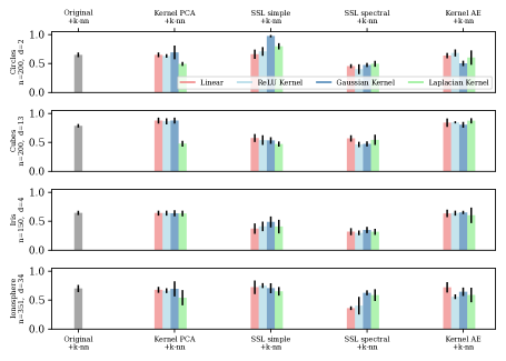
Figure 1: From left to right: we first consider $k$-nn on the original features followed by $k$-nn on embeddings obtained by Kernel PCA, and the proposed methods.

Comparing different embedding methods. Having observed that learning a representation before classification is beneficial, we now focus on the different embedding approaches. While the performed experiments do not reveal clear trends between different methods, we do note that the proposed methods overall perform on par or outperform Kernel PCA, underlining their relevance for kernel SSL.

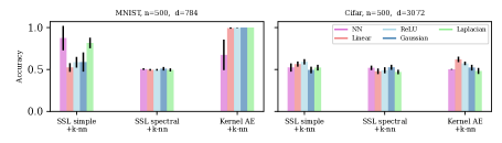
Figure 2: Comparison of kernel methods and neural network models for classification.

Comparison to Neural Networks for Classification and De-noising

Representation learning has mainly been established in the context of deep neural networks. In this paper, we make a step towards decoupling the representation learning paradigm from the widely used deep learning models. Nonetheless, we can still compare the proposed kernel methods to neural networks. We construct the corresponding NN model by replacing the linear function in the reproducing kernel Hilbert space, $\boldsymbol{W}^{\top}\phi({\boldsymbol{x}})$ by an one-hidden layer neural network $\boldsymbol{W}_{2}\sigma(\boldsymbol{W}_{1}{\boldsymbol{x}})$, where $\sigma(\cdot)$ is a non-linear activation function (and we still minimise a similar loss function).

Classification. We compare the performance of both representation learning approaches in Figure 2 for datasets CIFAR-10 (Krizhevsky, Hinton et al. 2009), as well as a subset of the first two classes of MNIST (Deng 2012) (i.e. $n=500$). We observe that the kernel methods perform on par with, or even outperform the neural networks. This indicates that there is not one dominant approach but one has to choose depending on the given task.

Figure 3: De-noising using NN AE with and Kernel AE.

Figure 4: Number of unlabelled points (classification).

De-Noising. As a second task, we consider de-noising using (Kernel) AE. Data is sampled from the first five classes of MNIST, CIFAR-10 and SVHN (Netzer et al. 2011) with $n=225$ and the noisy version are generated by $\overline{{\boldsymbol{x}}}:={\boldsymbol{x}}+\varepsilon,\leavevmode\nobreak\ \varepsilon_{i}\sim\mathcal{N}(0,0.1)$. We compare the performance of kernel-based approaches with the neural network reconstructions in Figure 3 by plotting the mean square error on the test set between the AE output and the clean data. Kernel AE outperforms the neural network AE in all considered settings. Moreover, there is little variation among the different kernels. This indicates that at least in the presented settings, the proposed kernel methods pose a viable alternative to traditional neural network based representation learning.

Formal connection between Kernel and neural network model. While it is known that regression with infinite-width networks is equivalent to kernel regression with neural tangent kernel (NTK) (Jacot, Gabriel, and Hongler 2018; Arora et al. 2019), similar results are not known for SSL and this brings up the question: Is kernel SSL equivalent to SSL with infinitely-wide neural networks? It is possible to show that single-layer Kernel AE with NTK is the infinite-width limit of over-parametrised AE (Nguyen, Wong, and Hegde 2021; Radhakrishnan, Belkin, and Uhler 2020). We believe that the same equivalence also holds for kernel contrastive learning (Definition 1) with NTK, but leave this as an open problem. We do not know if Definition 3 with NTK is the limit for bottleneck deep learning AE since, as we note earlier, there is no unique formulation for Kernel AE.

Discussions and Outlook

In this paper, we show that new variants of representer theorem allows one to rephrase SSL optimisation problems or the learned representations in terms of kernel functions. The resulting kernel SSL models provide natural tools for theoretical analysis. We believe that presented theory and method provide both scope for precise analysis of SSL and can also be extended to other SSL principles, such as other pretext tasks or joint embedding methods (Saunshi et al. 2019; Bardes, Ponce, and LeCun 2022; Grill et al. 2020; Chen and He 2020). We conclude with some additional discussions.

Computational limitations and small dataset setting. Exactly computing kernel matrices is not scalable, however random feature (RF) approximations of kernel methods are well suited for large data (Rahimi and Recht 2007; Carratino, Rudi, and Rosasco 2018). While one may construct scalable kernel representation learning methods using RF, it should be noted that RF models are lazy-trained networks (Ghorbani et al. 2019). So fully-trained deep representation learning models may be more suitable in such scenarios. However representation learning is relevant in all problems with availability of partially labelled data. This does not only apply to the big data regime where deep learning approaches are predominantly used, but also to small data settings where kernel methods are traditionally an important tool (Fernández-Delgado et al. 2014). The practical significance of developing kernel approaches is to broaden the scope of the representation learning paradigm beyond the deep learning community.

Kernel SSL vs. non-parametric data embedding. Several non-parametric generalisations of PCA, including functional PCA, kernel PCA, principle curves etc., have been studied over decades and could be compared to Kernel AEs. However, unlike kernel SSL, embedding methods are typically not inductive. As shown previously, the inductive representation learning by Kernel AE and contrastive learning make them suitable for downstream supervised tasks.

Kernel SSL vs. SSL with infinite-width neural networks. While it is known that regression with infinite-width networks is equivalent to kernel regression with neural tangent kernel (NTK) (Jacot, Gabriel, and Hongler 2018), similar results are not known for SSL. We believe that a study of the learning dynamics of neural network based SSL would show their equivalence with our kernel contrastive models with NTK. However, it is unclear to us whether a similar result can exist for kernel AE, as NTK approximations typically do not hold in the presence of bottleneck layers (Liu, Zhu, and Belkin 2020).

Appendix

In the supplementary material we provide the following additional proofs and results:

1. Model Illustration

2. Kernel Definitions

3. Representer Theorem

4. Further analysis of Kernel AE

5. Proofs for Kernel Methods at Optimal Parameterization

   1. Proof Theorem 4

   2. Proof Theorem 3

   3. Proof Theorem 5

6. Generalisation Error Bounds

   1. Proof Theorem 6

   2. Proof Theorem 7

   3. Generalisation Error on Downstream Task

7. Further Experiments

   1. Further discussion and experiments comparing neural networks and kernel approach

   2. Further experiments

Appendix A Model Illustration

In the following (Figure 5) we illustrate the main considered models: AE in the Kernel and neural network setting, Kernel PCA as well as the Kernel contrastive loss models schematically.

(a) Kernel AE and Kernel PCA. Data are mapped into a lower dimensional latent space and then reconstructed. (left) AE models: top shows the Kernel versions and bottom the traditional neural network formulation. The loss is computed between the original input ${\boldsymbol{x}}$ and the reconstruction $\widehat{{\boldsymbol{x}}}$. (right) Kernel PCA: Kernel PCA essentially performs PCA in the RKHS $\mathcal{H}$ (Schölkopf, Smola, and Müller 1998) and therefore computes distances in the feature space. We present an alternative reconstruction based formulation — Kernel Autoencoders (KAE) — that evaluate the reconstruction in the sample space instead of computing distances in the feature space. In comparison to Kernel PCA, this approach also provides a simple inference step for unseen datapoints.

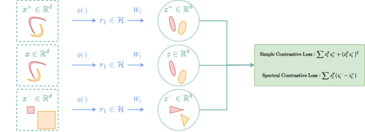
(b) Kernel Contrastive Loss. Considering a triplet setting, the reference (${\boldsymbol{x}}$), positive (${\boldsymbol{x}}^{+}$) and negative (${\boldsymbol{x}}^{-}$) are embedded into a latent space. The function is optimised by increasing the distance between embedding $\boldsymbol{z},\boldsymbol{z}^{-}$ and decreasing the distance between embedding of $\boldsymbol{z},\boldsymbol{z}^{+}$. We consider two different losses, that follow this basic idea.

Figure 5: Illustration of methods. Euclidean spaces and corresponding mappings are shown in green, RKHS and corresponding mappings in blue. (a) Overview over Reconstruction based approaches: traditional Kernel PCA, neural network based AE and Kernel AE (proposed new method). (b) Proposed method for self supervised representation learning using contrastive loss functions.

Appendix B Kernel Definitions

For completeness we include the definitions of the kernels considered in this paper below.

Definition 4 (Radial Basis Function (RBF) Kernel).

Let ${\boldsymbol{x}}$ and $\boldsymbol{y}$ be vectors, the the RBF kernel is defined as:

$$k({\boldsymbol{x}},\boldsymbol{y})=\exp\left(-\gamma\|{\boldsymbol{x}}-\boldsymbol{y}\|^{2}\right).$$

In the case $\gamma=\sigma^{-2}$ this becomes the Gaussian kernel of variance $\sigma^{2}$.

Definition 5 (Laplacian Kernel).

Similar to the RBF kernel, let ${\boldsymbol{x}}$ and $\boldsymbol{y}$ be vectors, then the Laplacian kernel is defined as:

$$k({\boldsymbol{x}},\boldsymbol{y})=\exp\left(-\gamma\|{\boldsymbol{x}}-\boldsymbol{y}\|_{1}\right).$$

Definition 6 (Linear Kernel).

Let ${\boldsymbol{x}}$ and $\boldsymbol{y}$ be vectors, then the linear kernel is defined as:

$$k({\boldsymbol{x}},\boldsymbol{y})={\boldsymbol{x}}^{\top}\boldsymbol{y}.$$

In addition to the above definitions that we consider in this paper the following definition illustrate that NTK inspired kernels such as the ReLU Kernel are also viable options to be considered as a ’pluck in option’ to the proposed models.

Definition 7 (ReLU Kernel (Bietti and Bach 2021)).

For a ReLU network with $L$ layers with inputs on the sphere, taking appropriate limits on the widths, one can show: $k_{\mathrm{NTK}}\left({\boldsymbol{x}},\boldsymbol{y}\right)=\kappa_{\mathrm{NTK}}^{L}\left({\boldsymbol{x}}^{\top}\boldsymbol{y}\right)$, with $\kappa_{\mathrm{NTK}}^{1}(\boldsymbol{u})=\kappa^{1}(\boldsymbol{u})=\boldsymbol{u}$ and for $\ell=2,\ldots,L$

$$\kappa^{\ell}(\boldsymbol{u}) =\kappa_{1}\left(\kappa^{\ell-1}(\boldsymbol{u})\right)$$

$$\kappa_{\mathrm{NTK}}^{\ell}(\boldsymbol{u}) =\kappa_{\mathrm{NTK}}^{\ell-1}(\boldsymbol{u})\kappa_{0}\left(\kappa^{\ell-1}(\boldsymbol{u})\right)+\kappa^{\ell}(\boldsymbol{u})$$

where

$$\kappa_{0}(u)= \frac{1}{\pi}(\pi-\arccos(u))$$

$$\kappa_{1}(u)= \frac{1}{\pi}\left(u\cdot(\pi-\arccos(u))+\sqrt{1-u^{2}}\right).$$

Appendix C Representer theorem

For convenience let us start by restating the theorem.

Given data $\boldsymbol{X}$ and an embedding dimension $h\in\mathbb{N}$, let $\mathcal{L}:\mathcal{H}^{h}\rightarrow\mathbb{R}$ be a loss function that vanishes on $\mathcal{H}^{\perp}_{X}$. Assume $\dim(\mathcal{H}_{X}^{\perp})\geq h$. Consider the following constrained minimisation problem over $\boldsymbol{w}_{1},\dots,\boldsymbol{w}_{h}\in\mathcal{H}$

$$\text{minimise }\mathcal{L}(\boldsymbol{w}_{1},\dots,\boldsymbol{w}_{h})$$ (8)

$$\text{ \leavevmode\nobreak\ s.t. \leavevmode\nobreak\ }\boldsymbol{W}^{*}\boldsymbol{W}=\boldsymbol{I}_{h}$$

Furthermore, consider the inequality-constrained problem over $\mathcal{H}_{X}$

$$\text{minimise }\mathcal{L}(\boldsymbol{w}_{1},\dots,\boldsymbol{w}_{h})$$ (9)

$$\text{ \leavevmode\nobreak\ s.t. \leavevmode\nobreak\ }\boldsymbol{W}^{T}\boldsymbol{W}\preceq\boldsymbol{I}_{h}\text{ and }\boldsymbol{w}_{1},\dots,\boldsymbol{w}_{h}\in\mathcal{H}_{X}$$

Then, every minimiser of (8) is contained in $\mathcal{H}_{X}^{h}$ if and only if every minimiser of (9) satisfies $\boldsymbol{W}^{T}\boldsymbol{W}=\boldsymbol{I}_{h}$.

Let us prove our characterization of loss functionals that admit representer theorems under orthonormality constraints. Denote $\boldsymbol{P}_{X}:\mathcal{H}\rightarrow\mathcal{H}_{X}$ for the projection onto the finite-dimensional subspace $\mathcal{H}_{X}$. Recall that $\boldsymbol{P}_{X}$ is a bounded linear operator with operator norm $\|\boldsymbol{P}_{X}\|=1$, satisfying $\boldsymbol{P}_{X}^{2}=\boldsymbol{P}_{X}$.

Proof.

Let us begin by assuming that a collection of functions $\boldsymbol{w}_{1},\dots,\boldsymbol{w}_{h}$ is a minimiser of

$$\text{minimise }\mathcal{L}(\boldsymbol{w}_{1},\dots,\boldsymbol{w}_{h})$$ (10)

$$\text{ \leavevmode\nobreak\ s.t. \leavevmode\nobreak\ }\boldsymbol{W}^{*}\boldsymbol{W}=\boldsymbol{I}_{h}$$

that is not contained in $\mathcal{H}_{X}$. Then, $\boldsymbol{P}_{X}\boldsymbol{w}_{1},\dots,\boldsymbol{P}_{X}\boldsymbol{w}_{h}\in\mathcal{H}_{X}$ achieve the same minimum, because $\mathcal{L}$ vanishes outside of $\mathcal{H}_{X}$. Because not all $\boldsymbol{w}_{1},\dots,\boldsymbol{w}_{h}$ are contained in $\mathcal{H}_{X}$, $\boldsymbol{W}^{*}\boldsymbol{W}\neq\boldsymbol{I}_{h}$. Thus, we have found a minimiser of

$$\text{minimise }\mathcal{L}(\boldsymbol{w}_{1},\dots,\boldsymbol{w}_{h})$$ (11)

$$\text{ \leavevmode\nobreak\ s.t. \leavevmode\nobreak\ }\boldsymbol{W}^{T}\boldsymbol{W}\preceq\boldsymbol{I}_{h}\text{ and }\boldsymbol{w}_{1},\dots,\boldsymbol{w}_{h}\in\mathcal{H}_{X}$$

that does not satisfy the constraint with equality. For the other direction, assume that there exists a minimiser $(\boldsymbol{w}_{1},\dots,\boldsymbol{w}_{h})\in\mathcal{H}_{X}$ of (11) that does not satisfy the constraint with equality. Then, exploiting the fact that $\dim(\mathcal{H}_{X}^{\perp})\geq h$, we can simply add $\boldsymbol{v}_{1},\dots,\boldsymbol{v}_{h}\in\mathcal{H}_{X}^{\perp}$ to $\boldsymbol{w}_{1},\dots,\boldsymbol{w}_{h}$ without changing $\mathcal{L}$, while at the same time ensuring $\langle\boldsymbol{w}_{i}+\boldsymbol{v}_{i},\boldsymbol{w}_{j}+\boldsymbol{v}_{j}\rangle=1_{i=j}$. This new minimiser of $\mathcal{L}$ is not contained in $\mathcal{H}_{X}$ and hence there is no representer theorem. ∎

Remark 3.

As mentioned in the main paper, checking that optimisers $\boldsymbol{W}$ of (11) are indeed orthonormal can be done by analyzing the behaviour of the loss functional $\mathcal{L}$ under orthonormalization of a given solution $\boldsymbol{W}$ with $\boldsymbol{W}^{T}\boldsymbol{W}\neq\boldsymbol{I}_{h}$. To illustrate this briefly in a finite-dimensional setting, consider the trace loss

$$\mathcal{L}(\boldsymbol{W})=-\operatorname{Tr}(\boldsymbol{W}^{T}\boldsymbol{A}\boldsymbol{W})$$

for some $\boldsymbol{A}\succeq 0$. If $\boldsymbol{W}^{T}\boldsymbol{W}\preceq\boldsymbol{I}_{h}$, then we can orthonormalize it via $\boldsymbol{X}=\boldsymbol{W}\boldsymbol{V}^{-1}$, where $\boldsymbol{V}\boldsymbol{V}^{T}=\boldsymbol{W}^{T}\boldsymbol{W}$. Then, $\boldsymbol{X}^{T}\boldsymbol{X}=\boldsymbol{I}_{h}$ and

$$\mathcal{L}(\boldsymbol{X})=\operatorname{Tr}(\boldsymbol{W}^{T}\boldsymbol{A}\boldsymbol{W}(\boldsymbol{V}\boldsymbol{V}^{T})^{-1})=\operatorname{Tr}(\boldsymbol{W}^{T}\boldsymbol{A}\boldsymbol{W}(\boldsymbol{W}^{T}\boldsymbol{W})^{-1})\leq\mathcal{L}(\boldsymbol{W})$$

where the final inequality follows from the fact that $\boldsymbol{W}^{T}\boldsymbol{W}\neq\boldsymbol{I}_{h}$.

Appendix D Further analysis of Kernel AE

Alternative formulations for the Kernel AE. As the overall idea of the paper is to translate deep SSL models to a kernel setting, we note at this point that there can be several ways to materialize this high level idea. Let us return to the ’bottleneck AE’. As mentioned in the main paper, when the chosen kernel is universal and $\lambda=0$, any arbitrary choice of $n$ distinct (even one-dimensional!) points $\boldsymbol{z}_{1},\dots,\boldsymbol{z}_{n}$ in the bottleneck achieves zero loss, in the sense that $\boldsymbol{Q}=\boldsymbol{X}$. This is in contradiction to the idea of finding a meaningful embedding of the data into lower dimensions, calling for some kind of regularization. Instead of the regularization of both $\boldsymbol{W}_{1}$ as well as $\boldsymbol{W}_{2}$, one could also consider the optimisation

$$\min_{\boldsymbol{Z},\boldsymbol{W}}\left\lVert\boldsymbol{X}-\boldsymbol{W}^{T}\phi(\boldsymbol{Z})\right\rVert^{2}+\lambda\cdot\left\lVert\boldsymbol{W}\right\rVert^{2}\text{ \leavevmode\nobreak\ s.t. \leavevmode\nobreak\ }\|\boldsymbol{z}_{i}\|^{2}=1\forall i\in[n]$$

which searches for a lower-dimensional embedding $\boldsymbol{Z}$ that maps smoothly to a given $\boldsymbol{X}$, by means of some $\boldsymbol{W}\in\mathcal{H}^{d}$. Moreover, an interesting connection to other kernel-based methods arises when we force the autoencoder to actually perfectly reconstruct the training data, i.e. when $\boldsymbol{Q}=\boldsymbol{Z}$. Then, the minimisation problem from Theorem 5 reduces to the problem

$$\min_{\boldsymbol{Z}}\operatorname{Tr}\left(\boldsymbol{Z}\boldsymbol{K}_{X}^{-1}\boldsymbol{Z}^{T}+\boldsymbol{X}\boldsymbol{K}_{Z}^{-1}\boldsymbol{X}^{T}\right)$$

$$\text{ \leavevmode\nobreak\ s.t. \leavevmode\nobreak\ }\|\boldsymbol{z}_{i}\|^{2}=1\leavevmode\nobreak\ \forall i\in[n]$$

Using the cyclic property of the trace, this becomes

$$\min_{\boldsymbol{Z}}\operatorname{Tr}\left(\boldsymbol{Z}^{T}\boldsymbol{Z}\boldsymbol{K}_{X}^{-1}\right)+\operatorname{Tr}\left(\boldsymbol{X}^{T}\boldsymbol{X}\boldsymbol{K}_{Z}^{-1}\right)$$

$$\text{ \leavevmode\nobreak\ s.t. \leavevmode\nobreak\ }\|\boldsymbol{z}_{i}\|^{2}=1\leavevmode\nobreak\ \forall i\in[n]$$

which allows us to recognize $\boldsymbol{Z}^{T}\boldsymbol{Z}=:\boldsymbol{L}_{Z}$ and $\boldsymbol{X}^{T}\boldsymbol{X}=:\boldsymbol{L}_{X}$ as kernel matrices for $\boldsymbol{Z}$ and $\boldsymbol{X}$ under the linear kernel $l(s,t)=\langle s,t\rangle$. Assuming for the moment that data is centered, above expression above can be viewed as simultaneously maximizing the Hilbert-Schmidt Independence Criterion (Gretton et al. 2005) between $\boldsymbol{L}_{X}$ and $\boldsymbol{K}_{Z}$, as well as $\boldsymbol{K}_{X}$ and $\boldsymbol{L}_{Z}$.

Appendix E Proofs for Kernel Methods at Optimal Parameterization

In this section we prove the kernel expressions at optimal parameterization.

Proof Theorem 3

For convenience let us start by restating the theorem.

Consider the optimisation problem as stated in Definition 1. Let $\boldsymbol{X},\boldsymbol{X}^{+},\boldsymbol{X}^{-}\in\mathbb{R}^{d\times n}$ denote the matrices corresponding to the anchors, positive and negative samples, respectively. Define the kernel matrices

$$\boldsymbol{K}=\left[k(x_{i},x_{j})\right]_{i,j} \boldsymbol{K}_{-}=\left[k(x_{i},x_{j}^{-})\right]_{i,j}$$

$$\boldsymbol{K}_{+}=\left[k(x_{i},x_{j}^{+})\right]_{i,j} \boldsymbol{K}_{--}=\left[k(x_{i}^{-},x_{j}^{-})\right]_{i,j}$$

$$\boldsymbol{K}_{++}=\left[k(x_{i}^{+},x_{j}^{+})\right]_{i,j} \boldsymbol{K}_{-+}=\left[k(x_{i}^{-},x_{j}^{+})\right]_{i,j}$$

Furthermore, define the matrices

$$\boldsymbol{K}_{\Delta}=\boldsymbol{K}_{--}+\boldsymbol{K}_{++}-\boldsymbol{K}_{-+}-\boldsymbol{K}_{-+}^{T} \boldsymbol{K}_{1}=\begin{bmatrix}\boldsymbol{K}&\boldsymbol{K}_{-}-\boldsymbol{K}_{+}\\ \boldsymbol{K}_{-}-\boldsymbol{K}_{+}&\boldsymbol{K}_{\Delta}\end{bmatrix}$$

$$\boldsymbol{B}=\begin{bmatrix}\boldsymbol{K}_{-}-\boldsymbol{K}_{+}\\ \boldsymbol{K}_{\Delta}\end{bmatrix}\cdot\begin{bmatrix}\boldsymbol{K}&\boldsymbol{K}_{-}-\boldsymbol{K}_{+}\\ \end{bmatrix} \boldsymbol{K}_{2}=-\frac{1}{2}\left(\boldsymbol{B}+\boldsymbol{B}^{T}\right)$$

Let $\boldsymbol{A}_{2}$ consist of the top $h$ eigenvectors of the matrix $\boldsymbol{K}_{1}^{-1/2}\boldsymbol{K}_{2}\boldsymbol{K}_{1}^{-1/2}$, and let $\boldsymbol{A}=\boldsymbol{K}_{1}^{-1/2}\boldsymbol{A}_{2}.$ Then at optimal parameterization, the embedding of any $x^{*}\in\mathbb{R}^{d}$ can be written in closed form as

$$\boldsymbol{z}^{*}=\boldsymbol{A}^{T}\begin{bmatrix}k(x^{*},\boldsymbol{X})\\ k(x^{*},\boldsymbol{X}^{-})-k(x^{*},\boldsymbol{X}^{+})\end{bmatrix}$$

Proof.

Define the (possibly infinite-dimensional) matrices $\Phi=[\phi(x_{1}),\dots,\phi(x_{n})]$ and $\Delta=[\phi(x_{1}^{-})-\phi(x_{1}^{+}),\dots,\phi(x_{n}^{-})-\phi(x_{n}^{+})]$, where $\phi:\mathbb{R}^{d}\rightarrow\mathcal{H}$ is the canonical feature map associated with the given kernel and $\mathcal{H}$ is the corresponding RKHS. We start by deriving the optimal parameterization. To do so recall the loss problem setup:

$$\min_{\boldsymbol{W}}\sum^{n}_{i=1}f(x_{i})^{T}\left(f(x_{i}^{-})-f(x_{i}^{+})\right)$$ (12)

$$\text{ \leavevmode\nobreak\ where \leavevmode\nobreak\ }f(x_{i})=\boldsymbol{W}^{T}\phi(x_{i})\text{ \leavevmode\nobreak\ s.t. \leavevmode\nobreak\ }\boldsymbol{W}^{*}\boldsymbol{W}=\boldsymbol{I}_{h}$$

By virtue of the representer theorem under orthonormality constraints, we may reduce this to a finite-dimensional optimisation problem on the span of $(\Phi,\Delta)$, change the constraints to $\boldsymbol{W}^{T}\boldsymbol{W}\preceq I_{h}$ for the moment, and finally verify that the optimal solution does in fact satisfy $\boldsymbol{W}^{T}\boldsymbol{W}=\boldsymbol{I}_{h}$. If that is the case, we know that this solution is also the minimiser of (12) over the entire space $\mathcal{H}$. Hence, let us assume that there exists $\boldsymbol{A}\in\mathbb{R}^{2n\times h}$ such that

$$\boldsymbol{W}=[\Phi,\Delta]\boldsymbol{A}$$

Thus, denoting $\boldsymbol{K}_{1}=[\Phi,\Delta]^{T}[\Phi,\Delta]\in\mathbb{R}^{2n\times 2n}$, we may rewrite our optimisation problem as

$$\min_{\boldsymbol{A}}\sum^{n}_{i=1}\phi(x_{i})^{T}[\Phi,\Delta]\boldsymbol{A}\boldsymbol{A}^{T}[\Phi,\Delta]^{T}\left(\phi(x_{i}^{-})-\phi(x_{i}^{+})\right)$$ (13)

$$\text{ \leavevmode\nobreak\ s.t. \leavevmode\nobreak\ }\boldsymbol{A}^{T}\boldsymbol{K}_{1}\boldsymbol{A}\preceq\boldsymbol{I}_{h}$$ (14)

This is equivalent to

$$\min_{\boldsymbol{A}}\operatorname{Tr}\left(\boldsymbol{A}^{T}[\Phi,\Delta]^{T}\Delta\Phi^{T}[\Phi,\Delta]\boldsymbol{A}\right)$$

$$\text{ \leavevmode\nobreak\ s.t. \leavevmode\nobreak\ }\boldsymbol{A}^{T}\boldsymbol{K}_{1}\boldsymbol{A}\preceq\boldsymbol{I}_{h}$$

Denoting $\boldsymbol{B}=[\Phi,\Delta]^{T}\Delta\Phi^{T}[\Phi,\Delta]$ and $\boldsymbol{K}_{2}=-\frac{1}{2}\left(\boldsymbol{B}+\boldsymbol{B}^{T}\right)$ for the negative symmetric part of $\boldsymbol{B}$, we are left with the trace maximization

$$\max_{\boldsymbol{A}}\operatorname{Tr}\left(\boldsymbol{A}^{T}\boldsymbol{K}_{2}\boldsymbol{A}\right)$$

$$\text{ \leavevmode\nobreak\ s.t. \leavevmode\nobreak\ }\boldsymbol{A}^{T}\boldsymbol{K}_{1}\boldsymbol{A}\preceq\boldsymbol{I}_{h}$$

Writing $\boldsymbol{A}_{2}=\boldsymbol{K}_{1}^{1/2}\boldsymbol{A}\in\mathbb{R}^{2n\times h}$, this simplifies to

$$\max_{\boldsymbol{A}_{2}}\operatorname{Tr}\left(\boldsymbol{A}_{2}^{T}\boldsymbol{K}_{1}^{-1/2}\boldsymbol{K}_{2}\boldsymbol{K}_{1}^{-1/2}\boldsymbol{A}_{2}\right)$$

$$\text{ \leavevmode\nobreak\ s.t. \leavevmode\nobreak\ }\boldsymbol{A}_{2}^{T}\boldsymbol{A}_{2}\preceq\boldsymbol{I}_{h}$$

This expression is maximized when $\boldsymbol{A}_{2}$ consists of the top $h$ orthonormal eigenvectors of $\boldsymbol{K}_{1}^{-1/2}\boldsymbol{K}_{2}\boldsymbol{K}_{1}^{-1/2}$, which do in fact satisfy $\boldsymbol{A}_{2}^{T}\boldsymbol{A}_{2}=\boldsymbol{I}_{h}$, and hence $\boldsymbol{W}=[\Phi,\Delta]\boldsymbol{A}$ also satisfies $\boldsymbol{W}^{T}\boldsymbol{W}=\boldsymbol{I}_{h}$ with equality. Note that both $\boldsymbol{K}_{1}$ and $\boldsymbol{K}_{2}$ depend only on inner products in the RKHS and can hence be computed directly from the kernel $k$, and that there is no need for evaluating the feature map directly. Finally, $\boldsymbol{A}=\boldsymbol{K}_{1}^{-1/2}\boldsymbol{A}_{2}$ becomes the desired minimiser of 13. For a new point ${\boldsymbol{x}}^{*}$, it holds that

$$f({\boldsymbol{x}}^{*}) =\boldsymbol{W}^{T}\phi({\boldsymbol{x}}^{*})$$

$$=\boldsymbol{A}^{T}[\Phi,\Delta]^{T}\phi({\boldsymbol{x}}^{*})$$

$$=\boldsymbol{A}^{T}\begin{bmatrix}k({\boldsymbol{x}}^{*},\boldsymbol{X})\\ k({\boldsymbol{x}}^{*},\boldsymbol{X}^{-})-k({\boldsymbol{x}}^{*},\boldsymbol{X}^{+})\end{bmatrix}$$

which again requires only knowledge of the kernel, and not of the (implicit) feature map. ∎

Proof Theorem 4

For convenience let us start by restating the theorem.

Consider the optimisation problem as stated in Definition 2, with $\boldsymbol{K}$ denoting the kernel matrix. Then, we can equivalently minimise the objective w.r.t. the embeddings $\boldsymbol{Z}\in\mathbb{R}^{h\times 3n}$. Denoting by $\boldsymbol{z}_{1},\dots,\boldsymbol{z}_{3n}$ the columns of $\boldsymbol{Z}$, the loss to be minimised becomes

$$\min_{\boldsymbol{Z}\in\mathbb{R}^{h\times 3n}}\sum^{n}_{i=1}-2\boldsymbol{z}_{i}^{T}\boldsymbol{z}_{i+n}+\left(\boldsymbol{z}_{i}^{T}\boldsymbol{z}_{i+2n}\right)^{2}+\lambda\cdot\operatorname{Tr}\left(\boldsymbol{Z}\boldsymbol{K}^{-1}\boldsymbol{Z}^{T}\right)$$

The gradient of the loss function in terms of $\boldsymbol{Z}$ is therefore given by

$$2\lambda\boldsymbol{Z}\boldsymbol{K}^{-1}+\begin{cases}-2\boldsymbol{z}_{i+n}+2(\boldsymbol{z}_{i}^{T}\boldsymbol{z}_{i+2n})\boldsymbol{z}_{i+2n}&,i\in[n]\\ -2\boldsymbol{z}_{i-n}&,i\in[n+1,2n]\\ 2(\boldsymbol{z}_{i}^{T}\boldsymbol{z}_{i-2n})z_{i-2n}&,i\in[2n+1,3n]\end{cases}$$

For any new point ${\boldsymbol{x}}^{*}\in\mathbb{R}^{d}$, the trained model maps it to

$$\boldsymbol{z}^{*}:=\boldsymbol{Z}\boldsymbol{K}^{-1}k(\boldsymbol{X},{\boldsymbol{x}}^{*}).$$

Proof.

Recall that in contrastive learning with the spectral contrastive loss, we learn a representation of the form $f_{\boldsymbol{W}}({\boldsymbol{x}})=\boldsymbol{W}^{T}\phi({\boldsymbol{x}})=\left(\boldsymbol{w}_{1}(x),\dots,\boldsymbol{w}_{h}(x)\right)$ by optimising the following objective function:

$$\mathcal{L}^{\mathrm{Sp}}:=\sum^{n}_{i=1}-2f_{\boldsymbol{W}}({\boldsymbol{x}}_{i})^{T}f_{\boldsymbol{W}}({\boldsymbol{x}}_{i}^{+})+\left(f_{\boldsymbol{W}}({\boldsymbol{x}}_{i})^{T}f_{\boldsymbol{W}}({\boldsymbol{x}}_{i}^{-})\right)^{2}+\lambda\left\lVert\boldsymbol{W}\right\rVert^{2}_{\mathcal{H}}.$$

Since the term $\sum^{n}_{i=1}-2f_{\boldsymbol{W}}({\boldsymbol{x}}_{i})^{T}f_{\boldsymbol{W}}({\boldsymbol{x}}_{i}^{+})+\left(f_{\boldsymbol{W}}({\boldsymbol{x}}_{i})^{T}f_{\boldsymbol{W}}({\boldsymbol{x}}_{i}^{-})\right)^{2}$ vanishes for any choice of $\boldsymbol{w}_{1},\dots,\boldsymbol{w}_{h}\in\mathcal{H}_{X}^{\perp}$, and we add a norm regularization to this objective function, it is clear by the representer theorem that any minimiser of $\mathcal{L}^{\mathrm{Sp}}$ must consist of $h$ functions from $\mathcal{H}_{X}$. We may hence write $\boldsymbol{w}_{j}=\Phi\boldsymbol{a}_{j}$ for some $\boldsymbol{a}_{j}\in\mathbb{R}^{n}$. Denoting $\boldsymbol{Z}$ for the embeddings under the map $\boldsymbol{W}^{T}\phi({\boldsymbol{x}}_{i})$ and $\boldsymbol{A}$ for the matrix with columns $\boldsymbol{a}_{1},\dots,\boldsymbol{a}_{h}$, we see that for any $j\in[h]$, it must hold that $\boldsymbol{A}^{T}\boldsymbol{K}=\boldsymbol{Z}$ and hence $\boldsymbol{A}=\boldsymbol{K}^{-1}\boldsymbol{Z}^{T}$. Thus, $\boldsymbol{W}=\Phi\boldsymbol{K}^{-1}\boldsymbol{Z}^{T}$ and $\|\boldsymbol{W}\|^{2}=\operatorname{Tr}(\boldsymbol{Z}\boldsymbol{K}^{-1}\boldsymbol{K}\boldsymbol{K}^{-1}\boldsymbol{Z}^{T})=\operatorname{Tr}(\boldsymbol{Z}\boldsymbol{K}^{-1}\boldsymbol{Z}^{T})$. This allows us to reformulate the minimisation problem as an optimisation over the embedded points $\boldsymbol{Z}$, yielding the gradients

$$\nabla\mathcal{L}^{\mathrm{Sp}}=2\lambda\boldsymbol{Z}\boldsymbol{K}^{-1}+\begin{cases}-2\boldsymbol{z}_{i+n}+2(\boldsymbol{z}_{i}^{T}\boldsymbol{z}_{i+2n})\boldsymbol{z}_{i+2n}&,i\in[n]\\ -2\boldsymbol{z}_{i-n}&,i\in[n+1,2n]\\ 2(\boldsymbol{z}_{i}^{T}\boldsymbol{z}_{i-2n})z_{i-2n}&,i\in[2n+1,3n]\end{cases}$$

Finally, by virtue of our choice of $\boldsymbol{W}=\Phi\boldsymbol{K}^{-1}\boldsymbol{Z}^{T}$, any new point ${\boldsymbol{x}}^{*}\in\mathbb{R}^{d}$ is mapped to

$$\boldsymbol{z}^{*}:=\boldsymbol{Z}\boldsymbol{K}^{-1}k(\boldsymbol{X},{\boldsymbol{x}}^{*}).$$

∎

Proof Theorem 5

For convenience let us start by restating the theorem.

For any bottleneck $\boldsymbol{Z}\in\mathbb{R}^{h\times n}$, define the reconstruction

$$\boldsymbol{Q}(\boldsymbol{Z})=\boldsymbol{X}(\boldsymbol{K}_{Z}+\lambda I_{n})^{-1}\boldsymbol{K}_{Z}$$

Learning the Kernel AE from Definition 3 is then equivalent to minimising the following expression over all possible embeddings $\boldsymbol{Z}\in\mathbb{R}^{h\times n}$:

$$\|\boldsymbol{Q}(Z)-\boldsymbol{X}\|^{2}+\lambda\operatorname{Tr}\left(\boldsymbol{Z}\boldsymbol{K}_{X}^{-1}\boldsymbol{Z}^{T}+\boldsymbol{Q}\boldsymbol{K}_{Z}^{-1}\boldsymbol{Q}^{T}\right)$$

$$\text{ \leavevmode\nobreak\ s.t. \leavevmode\nobreak\ }\|\boldsymbol{z}_{i}\|^{2}=1\leavevmode\nobreak\ \forall i\in[n].$$

Given $\boldsymbol{Z}$, any new ${{\boldsymbol{x}}}^{*}\in\mathbb{R}^{d}$ is embedded in the bottleneck as

$$\boldsymbol{z}^{*}=\boldsymbol{Z}\boldsymbol{K}_{X}^{-1}k({{\boldsymbol{x}}}^{*},{\boldsymbol{X}})$$

and reconstructed as

$$\hat{{\boldsymbol{x}}}^{*} =\boldsymbol{X}\left(\boldsymbol{K}_{Z}+\lambda\boldsymbol{I}_{n}\right)^{-1}k(\boldsymbol{z}^{*},\boldsymbol{Z})$$

Proof.

Writing $\boldsymbol{Z}=[z_{1},\dots,z_{n}]\in\mathbb{R}^{h\times n}$ for the points in the bottleneck and $\boldsymbol{Q}=[q_{1},\dots,q_{n}]\in\mathbb{R}^{d\times n}$ for the points in the output layer, and denoting $\Phi_{X},\Phi_{Z},\boldsymbol{K}_{X},\boldsymbol{K}_{Z}$ for the respective feature maps and kernel matrices of inputs $\boldsymbol{X}$ and bottleneck $\boldsymbol{Z}$, the representer theorem (with norm regularization) and the same argument as in the proof of Theorem 4 yields that the minimum-norm $\boldsymbol{W}_{1}$ and $\boldsymbol{W}_{2}$ satisfying $\boldsymbol{W}_{1}^{T}\Phi_{X}=\boldsymbol{Z}$ and $\boldsymbol{W}_{2}^{T}\Phi_{Z}=\boldsymbol{Q}$ are given by

$$\boldsymbol{W}_{1}=\Phi_{X}\boldsymbol{K}_{X}^{-1}\boldsymbol{Z}^{T}$$

$$\boldsymbol{W}_{2}=\Phi_{Z}\boldsymbol{K}_{Z}^{-1}\boldsymbol{Q}^{T}$$

Their Frobenius norms (in the infinite-dimensional case, their Hilbert-Schmidt norms) are

$$\left\lVert\boldsymbol{W}_{1}\right\rVert^{2}=\operatorname{Tr}(\boldsymbol{Z}\boldsymbol{K}_{X}^{-1}\boldsymbol{Z}^{T})$$

$$\left\lVert\boldsymbol{W}_{2}\right\rVert^{2}=\operatorname{Tr}(\boldsymbol{Q}\boldsymbol{K}_{Z}^{-1}\boldsymbol{Q}^{T})$$

Thus, the loss function is equivalent to minimising the expression

$$\min_{\boldsymbol{Z},\boldsymbol{Q}}\left\lVert\boldsymbol{X}-\boldsymbol{Q}\right\rVert^{2}+\lambda\cdot\operatorname{Tr}(\boldsymbol{Z}\boldsymbol{K}_{X}^{-1}\boldsymbol{Z}^{T}+\boldsymbol{Q}\boldsymbol{K}_{Z}^{-1}\boldsymbol{Q}^{T})$$

$$\text{ \leavevmode\nobreak\ s.t. \leavevmode\nobreak\ }\|\boldsymbol{z}_{i}\|^{2}=1\text{ \leavevmode\nobreak\ for all \leavevmode\nobreak\ }i\in[n]$$

Observe that for any fixed bottleneck $\boldsymbol{Z}$, $\operatorname{Tr}(\boldsymbol{Z}\boldsymbol{K}_{X}^{-1}\boldsymbol{Z}^{T})$ remains constant and the above problem reduces to a sum of $d$ kernel ridge regressions, with labels $\boldsymbol{X}$ and observations $\boldsymbol{Z}$. Thus, the optimal parameterization $\boldsymbol{W}_{2}$ simplifies to

$$\boldsymbol{W}_{2}=\Phi_{Z}\left(\boldsymbol{K}_{Z}+\lambda\boldsymbol{I}_{n}\right)^{-1}\boldsymbol{X}^{T}$$

and directly implies the final layer

$$\boldsymbol{Q}=\boldsymbol{X}\left(\boldsymbol{K}_{Z}+\lambda\boldsymbol{I}_{n}\right)^{-1}\boldsymbol{K}_{Z}$$

Learning the Kernel AE from Definition 3 is hence equivalent to minimising the following expression over all possible embeddings $\boldsymbol{Z}\in\mathbb{R}^{h\times n}$:

$$\|\boldsymbol{Q}(Z)-\boldsymbol{X}\|^{2}+\lambda\operatorname{Tr}\left(\boldsymbol{Z}\boldsymbol{K}_{X}^{-1}\boldsymbol{Z}^{T}+\boldsymbol{Q}\boldsymbol{K}_{Z}^{-1}\boldsymbol{Q}^{T}\right)$$

$$\text{ \leavevmode\nobreak\ s.t. \leavevmode\nobreak\ }\|\boldsymbol{z}_{i}\|^{2}=1\leavevmode\nobreak\ \forall i\in[n].$$

Given $\boldsymbol{Z}$, any new ${{\boldsymbol{x}}}^{*}\in\mathbb{R}^{d}$ is embedded in the bottleneck as

$$\boldsymbol{z}^{*}=\boldsymbol{Z}\boldsymbol{K}_{X}^{-1}k({{\boldsymbol{x}}}^{*},{\boldsymbol{X}})$$

and reconstructed as

$$\hat{{\boldsymbol{x}}}^{*} =\boldsymbol{X}\left(\boldsymbol{K}_{Z}+\lambda\boldsymbol{I}_{n}\right)^{-1}k(\boldsymbol{z}^{*},\boldsymbol{Z})$$

∎

Appendix F Generalisation Error Bounds

Before going into the proofs of the generalisation error bounds we recall the form of generalisation error bounds we are interested in. In general would be interested in characterizing the risk in expectation over the data

$$\mathcal{L}(f)=\underset{\boldsymbol{X}\sim\mathcal{D}}{\mathbb{E}}\left[l\left(f(\boldsymbol{X})\right)\right].$$

However since we do not have access to $\mathcal{D}$ we can only obtain the empirical risk quantity

$$\widehat{\mathcal{L}}(f)=\frac{1}{n}\sum_{i=1}^{n}l\left(f(\boldsymbol{X}_{i})\right).$$

Therefore we characterize the generalisation error as

$$\mathcal{L}(f)\leq\widehat{\mathcal{L}}(f)+\text{complexity term}+\text{slack term}$$ (15)

where we will consider Rademacher based characterizations of the complexity term.

Proof Theorem 6

For convenience let us start by restating the theorem.

Let $\mathcal{F}:=\left\{{\boldsymbol{X}}\mapsto\boldsymbol{W}^{T}\phi\left({\boldsymbol{X}}\right):\|\boldsymbol{W}^{T}\|_{\mathcal{H}}\leq\omega\right\}$ be the class of embedding functions we consider in the contrastive setting. Define $\alpha:=\left(\sqrt{h\operatorname{Tr}\left[\boldsymbol{K}_{\boldsymbol{X}}\right]}+\sqrt{h\operatorname{Tr}\left[\boldsymbol{K}_{\boldsymbol{X}^{-}}\right]}+\sqrt{h\operatorname{Tr}\left[\boldsymbol{K}_{\boldsymbol{X}^{+}}\right]}\right)$ as well as $\kappa:=\max_{{\boldsymbol{x}}^{\prime}_{i}\in\{{\boldsymbol{x}}_{i},{\boldsymbol{x}}_{i}^{-},{\boldsymbol{x}}_{i}^{+}\}_{i=1}^{n}}k({\boldsymbol{x}}^{\prime}_{i},{\boldsymbol{x}}^{\prime}_{i})$. We then obtain the generalisation error for the proposed losses as follows.

1. Simple Contrastive Loss. Let the loss be given by Definition 1. Then, for any $\delta>0$, the following statement holds with probability at least $1-\delta$ for any $f\in\mathcal{F}$:

   $$\mathcal{L}^{\mathrm{Si}}\leq\widehat{\mathcal{L}}^{\mathrm{Si}}+O\left(\frac{\omega^{2}\sqrt{\kappa}\alpha}{n}+\omega^{2}\kappa\sqrt{\frac{\log\frac{1}{\delta}}{n}}\right)$$

2. Spectral Contrastive Loss. Let the loss be given by Definition 2. Then, for any $\delta>0$, the following statement holds with probability at least $1-\delta$ for any $f\in\mathcal{F}$:

   $$\mathcal{L}^{{Sp}}\leq\widehat{\mathcal{L}}^{{Sp}}+O\left(\lambda\omega^{2}+\frac{\omega^{3}\kappa^{\frac{3}{2}}\alpha}{n}+\omega^{4}\kappa^{2}\sqrt{\frac{\log\frac{1}{\delta}}{n}}\right)$$

We will proof the two bounds separately.

Proof.

Part 1. Simple Contrastive Loss. We start from the following Lemma, that is defined in the context of the simple contrastive loss:

Lemma 1 ((Saunshi et al. 2019)).

With probability at least $1-\delta$ over the training set, $\forall f\in\mathcal{F}$:

$$\mathcal{L}_{un}\leq\widehat{\mathcal{L}}_{un}+O\left(R\frac{\mathfrak{R}_{c}(\mathcal{F},\mathbf{x})}{n}+B\sqrt{\frac{\log\frac{1}{\delta}}{n}}\right)$$

where $\left\lVert f(\cdot)\right\rVert\leq R$ and $B$ the bound on the loss function wich in the case of the simple contrastive loss can be given by $B=O(R^{2})$.

Furthermore the the Rademacher complexity term in the above lemma is defined over the following definition.

Definition 8 (Expected Rademacher Complexity for Contrastive Setting (following Saunshi et al. (2019))).

Let our dataset be consistent of triplets $\mathcal{S}=\left\{{\boldsymbol{x}}_{i},{\boldsymbol{x}}_{i}^{+},{\boldsymbol{x}}_{i}^{-}\right\}_{i=1}^{n}$ and $f_{\mid\mathcal{S}}=\left(f_{t}\left(x_{j}\right),f_{t}\left(x_{j}^{+}\right),f_{t}\left(x_{j}^{-}\right)\right)_{j\in[n],t\in[h]}\in\mathbb{R}^{3hn}$ be the restriction of and $f\in\mathcal{F}$ to $S$, then we define the empirical Rademacher Complexity as

$$\mathfrak{R}_{c}(\mathcal{F},\mathbf{x})=\underset{{\sigma\sim\{\pm 1\}^{3nh}}}{\mathbb{E}}\left[\sup_{f\in\mathcal{F}}\sum_{i=1}^{3dn}\sigma_{i}f_{\mid\mathcal{S}}\left(x_{i}\right)\right].$$

Having the setup complete we can now compute the complexity term of the in this paper considered kernel function. In the first step we pluck in our considered model and split it up by the reference, positive and negative samples:

$$\mathfrak{R}_{c}(\mathcal{F},\mathbf{x}) =\underset{{\sigma\sim\{\pm 1\}^{3nd}}}{\mathbb{E}}\left[\sup_{f\in\mathcal{F}}\sum_{i=1}^{3hn}\sigma_{i}f_{\mid\mathcal{S}}\left(x_{i}\right)\right]$$

$$=\underset{{\sigma\sim\{\pm 1\}^{3nd}}}{\mathbb{E}}\left[\sup_{\boldsymbol{W}:\left\lVert\boldsymbol{W}\right\rVert_{\mathcal{H}}\leq\omega}\sum_{j=1}^{h}\sum_{i=1}^{n}\sigma_{i}\boldsymbol{W}_{\cdot,j}^{T}\phi\left({{\boldsymbol{x}}_{i}}\right)+\sigma_{i+n}\boldsymbol{W}_{\cdot,j}^{T}\phi\left({{\boldsymbol{x}}^{-}_{i}}\right)+\sigma_{i+2n}\boldsymbol{W}_{\cdot,j}^{T}\phi\left({{\boldsymbol{x}}^{+}_{i}}\right)\right]$$

$$\leq\omega\left(\underset{\sigma}{\mathbb{E}}\left[h\left\lVert\sum_{i=1}^{n}\sigma_{i}\phi\left({{\boldsymbol{x}}_{i}}\right)\right\rVert\right]+\underset{\sigma}{\mathbb{E}}\left[h\left\lVert\sum_{i=1}^{n}\sigma_{i}\phi\left({{\boldsymbol{x}}^{-}_{i}}\right)\right\rVert\right]+\underset{\sigma}{\mathbb{E}}\left[h\left\lVert\sum_{i=1}^{n}\sigma_{i}\phi\left({{\boldsymbol{x}}^{+}_{i}}\right)\right\rVert\right]\right)$$ (by linearity of expectation and Cauchy-Schwartz inequality)

$$=\omega\left(\underset{\sigma}{\mathbb{E}}\left[\sqrt{h\left\lVert\sum_{i=1}^{n}\sigma_{i}\phi\left({{\boldsymbol{x}}_{i}}\right)\right\rVert^{2}}\right]+\underset{\sigma}{\mathbb{E}}\left[\sqrt{h\left\lVert\sum_{i=1}^{n}\sigma_{i}\phi\left({{\boldsymbol{x}}^{-}_{i}}\right)\right\rVert^{2}}\right]+\underset{\sigma}{\mathbb{E}}\left[\sqrt{h\left\lVert\sum_{i=1}^{n}\sigma_{i}\phi\left({{\boldsymbol{x}}^{+}_{i}}\right)\right\rVert^{2}}\right]\right)$$

$$\leq\omega\left(\sqrt{h\underset{\sigma}{\mathbb{E}}\left[\left\lVert\sum_{i=1}^{n}\sigma_{i}\phi\left({{\boldsymbol{x}}_{i}}\right)\right\rVert^{2}\right]}+\sqrt{h\underset{\sigma}{\mathbb{E}}\left[\left\lVert\sum_{i=1}^{n}\sigma_{i}\phi\left({{\boldsymbol{x}}^{-}_{i}}\right)\right\rVert^{2}\right]}+\sqrt{h\underset{\sigma}{\mathbb{E}}\left[\left\lVert\sum_{i=1}^{n}\sigma_{i}\phi\left({{\boldsymbol{x}}^{+}_{i}}\right)\right\rVert^{2}\right]}\right)$$ (Jensen’s inequality)

$$=\omega\left(\sqrt{h\operatorname{Tr}\left[\boldsymbol{K}_{\boldsymbol{X}}\right]}+\sqrt{h\operatorname{Tr}\left[\boldsymbol{K}_{\boldsymbol{X}^{-}}\right]}+\sqrt{h\operatorname{Tr}\left[\boldsymbol{K}_{\boldsymbol{X}^{+}}\right]}\right).$$

Secondly we have to bound the quantity $\left\lVert f(\cdot)\right\rVert\leq R$:

$$\left\lVert f(\cdot)\right\rVert =\left\lVert\boldsymbol{W}^{T}\phi({\boldsymbol{x}})\right\rVert$$ (by definition of considered embedding function)

$$\leq\left\lVert\boldsymbol{W}^{T}\right\rVert\left\lVert\phi({\boldsymbol{x}})\right\rVert$$

$$\leq\omega\left\lVert\phi({\boldsymbol{x}})\right\rVert \left\lVert\boldsymbol{W}^{T}\right\rVert$$ (by definition of function class is bound)

$$\leq\omega\sqrt{\langle\phi({\boldsymbol{x}})^{T}\phi({\boldsymbol{x}})\rangle}$$

$$\leq\omega\sqrt{\max_{{\boldsymbol{x}}_{i}}.k({\boldsymbol{x}}_{i},{\boldsymbol{x}}_{i})} {\boldsymbol{x}}_{i}$$ (bounding over all possible )

Defining $\kappa:=\max_{{\boldsymbol{x}}^{\prime}_{i}\in\{{\boldsymbol{x}}_{i},{\boldsymbol{x}}_{i}^{-},{\boldsymbol{x}}_{i}^{+}\}_{i=1}^{n}}k({\boldsymbol{x}}^{\prime}_{i},{\boldsymbol{x}}^{\prime}_{i})$ to account for reference, positive and negative samples and combining all results concludes this part of the proof. ∎

Proof.

Part 2. Spectral Contrastive Loss.

The overall proof structure follows the one presented above for the simple contrastive loss, however Lemma 1 is define for the simple contrastive loss. Therefore we will adept the proof of Saunshi et al. (2019) Lemma A.2. to obtain the following lemma for the spectral contrastive loss.

Lemma 2.

With probability at least $1-\delta$ over the training set, $\forall f\in\mathcal{F}$:

$$\mathcal{L}_{un}\leq\widehat{\mathcal{L}}_{un}+O\left(R^{3}\frac{\mathfrak{R}_{c}(\mathcal{F},\mathbf{x})}{n}+B\sqrt{\frac{\log\frac{1}{\delta}}{n}}\right)$$ (16)

where $\mathfrak{R}_{c}(\mathcal{F},\mathbf{x})$ is the Vector Rademacher Complexity where $\left\lVert f(\cdot)\right\rVert\leq R$ and $B=O(R^{4})$.

Before proofing Lemma 2 we first recall the following Lemma:

Lemma 3 (Corollary 4 in (Maurer 2016)).

Let $Z$ be any set and $\mathcal{S}=\{z_{j}\}^{n}_{j=1}\in Z^{n}$. Let $\widetilde{\mathcal{F}}$ be a class of functions $\tilde{f}:Z\rightarrow\mathbb{R}^{d}$ and $h:\mathbb{R}^{d}\rightarrow\mathbb{R}$ be $L$-Lipschitz. For all $\tilde{f}\in\widetilde{\mathcal{F}}$, let $g_{\tilde{f}}=h\circ\tilde{f}$. Then

$$\underset{\sigma\sim\{\pm 1\}^{n}}{\mathbb{E}}\left[\sup_{\tilde{f}\in\tilde{\mathcal{F}}}\left\langle\sigma,\left(g_{\tilde{f}}\right)_{\mid\mathcal{S}}\right\rangle\right]\leq\sqrt{2}L\underset{\sigma\sim\{\pm 1\}^{dn}}{\mathbb{E}}\left[\sup_{\tilde{f}\in\tilde{\mathcal{F}}}\left\langle\sigma,\tilde{f}_{\mid\mathcal{S}}\right\rangle\right]$$ (17)

where $\tilde{f}_{\mid\mathcal{S}}=\left(\tilde{f}_{t}\left(z_{j}\right)\right)_{t\in[d],j\in[n]}$.

We start by considering the classical Rademacher complexity based generalization error. For a real function class $\mathcal{G}$ whose functions map from a set $Z$ to $[0,1]$ and for any $\delta>0$, if $\mathcal{S}$ is a training set composed by $n$ i.i.d. samples $\{z_{j}\}_{j=1}^{n}$, then with probability at least $1-\frac{2}{\delta}$,for all $g\in\mathcal{G}$

$$\mathbb{E}[g(z)]\leq\frac{1}{n}\sum_{j=1}^{n}g\left(z_{i}\right)+\frac{2\mathfrak{R}_{\mathcal{S}}(\mathcal{G})}{n}+3\sqrt{\frac{\log\frac{4}{\delta}}{2n}}$$

where $\mathfrak{R}_{\mathcal{S}}(G)$ is the standard Rademacher complexity. We can apply this to our setting by considering $Z=\mathcal{X}^{3}$ and defining the function class as

$$\mathcal{G}=\left\{g_{f}\left(x,x^{+},x^{-}\right)=\frac{1}{B}\left(f(x)^{T}f\left(x^{+}\right)-\left(f\left(x_{i}\right)^{T}f\left(x_{i}^{-}\right)\right)^{2}\right)\mid f\in\mathcal{F}\right\}.$$

Now to show (16) consider some universal constant $c$ we have to show $\mathfrak{R}_{\mathcal{S}}(\mathcal{G})\leq c\frac{R^{3}}{B}\mathfrak{R}_{\mathcal{S}}(\mathcal{G})$ or equivalently

$$\underset{\sigma\sim\{\pm 1\}^{n}}{\mathbb{E}}\left[\sup_{f\in\mathcal{F}}\left\langle\sigma,\left(g_{f}\right)_{\mid\mathcal{S}}\right\rangle\right]\leq c\frac{R^{3}}{B}\underset{\sigma\sim\{\pm 1\}^{3dn}}{\mathbb{E}}\left[\sup_{f\in\mathcal{F}}\left\langle\sigma,f_{\mid\mathcal{S}}\right\rangle\right]$$ (18)

where $\left(g_{f}\right)_{\mid\mathcal{S}}=\left\{g_{f}\left(x_{j},x_{j}^{+},x_{1}^{-}\right)\right\}_{j=1}^{n}$. We can now observe by setting $Z=\mathcal{X}^{3},b=3d$ and

$$\widetilde{\mathcal{F}}=\left\{\tilde{f}\left(x,x^{+},x^{-}\right)=\left(f(x),f\left(x^{+}\right),f\left(x^{-}\right),\right)\mid f\in\mathcal{F}\right\}$$

and using $g_{\tilde{f}}=g_{f}$ that (17) and (18) exactly coincide and we need to show $L\leq\frac{c}{\sqrt{2}}\frac{R^{3}}{B}$ for some constant $c$. Now for $z=(x,x^{+},x^{-})$ we have $g_{\tilde{f}}(z)=\frac{1}{B}\psi(\tilde{f}(z))$ where $\psi:\mathbb{R}^{(1+2)d}\rightarrow\mathbb{R}$ with $\psi\left(\left(v_{t},v_{t}^{+},v_{t}^{-}\right)_{t\in[d]}\right)=\sum_{t}-v_{t}v_{t}^{+}+\left(v_{t}v_{t}^{-}\right)^{2}.$ We can now show that $\psi$ is $R^{3}$ lipschitz where $\sum_{t}v_{t}^{2},\sum_{t}\left(v_{t}^{+}\right)^{2},\sum_{t}\left(v_{t}^{-}\right)^{2}\leq R^{2}$ by computing its Jacobian. To do so we derive $\frac{\partial\psi_{i}}{\partial v_{t}^{+}}=-v_{t}\quad\frac{\partial\psi_{i}}{\partial v_{t}}=-v_{t}^{+}+v_{t}^{-}v_{t}^{-}v_{t}$ and $\frac{\partial\psi_{i}}{\partial v_{t}^{-}}=v_{t}v_{t}v_{t}^{-}$ and get by triangle inequality the Frobenius norm on the Jacobian $\boldsymbol{J}$ of $\psi$ $\left\lVert\boldsymbol{J}\right\rVert_{F}\leq\sqrt{\sum_{t}(v_{t}^{-})^{4}(v_{t})^{2}+(v_{t}^{-})^{3}v_{t}^{3}+(v_{t}^{-})^{2}v_{t}^{4}+(v_{t}^{+})^{2}+(v_{t}^{+})v_{t}+(v_{t})^{2}}=O(R^{3}).$ Finally using $\left\lVert\boldsymbol{J}\right\rVert_{2}\leq\left\lVert\boldsymbol{J}\right\rVert_{F}$ bounds the lipschitzness and concludes the proof of Lemma 2.

As the function class we consider for embedding does not change $(\mathcal{F}:=\left\{{\boldsymbol{X}}\mapsto\boldsymbol{W}^{T}\phi\left({\boldsymbol{X}}\right):\|\boldsymbol{W}^{T}\|_{\mathcal{H}}\leq\omega\right\})$, we again obtain $\mathfrak{R}_{c}(\mathcal{F},\mathbf{x})\leq\omega\left(\sqrt{h\operatorname{Tr}\left[\boldsymbol{K}_{\boldsymbol{X}}\right]}+\sqrt{h\operatorname{Tr}\left[\boldsymbol{K}_{\boldsymbol{X}^{-}}\right]}+\sqrt{h\operatorname{Tr}\left[\boldsymbol{K}_{\boldsymbol{X}^{+}}\right]}\right)$ and $\omega\sqrt{\kappa}\leq R,$ which combined with the above Lemma 2 concludes the proof. ∎

Proof Theorem 7

For convenience let us start by restating the theorem.

Assume the optimisation be given by Definition 3and define the class of encoders/decoders as: $\mathcal{F}:=\big{\{}{\boldsymbol{X}}\mapsto\boldsymbol{W}_{2}^{T}\phi_{2}\left(\boldsymbol{W}_{1}^{T}\phi_{1}\left({\boldsymbol{X}}\right)\right)\text{ \leavevmode\nobreak\ s.t. \leavevmode\nobreak\ }\|\boldsymbol{W}_{1}^{T}\phi({\boldsymbol{x}}_{i})\|^{2}=1\leavevmode\nobreak\ \forall\leavevmode\nobreak\ i\in[n]\leavevmode\nobreak\ :\leavevmode\nobreak\ \|\boldsymbol{W}_{1}^{T}\|_{\mathcal{H}}\leq\omega_{1},\|\boldsymbol{W}_{2}^{T}\|_{\mathcal{H}}\leq\omega_{2}\big{\}}$. Let $\gamma=\max_{\boldsymbol{s}\in\mathbb{R}^{h}\text{ \leavevmode\nobreak\ s.t. \leavevmode\nobreak\ }\left\lVert\boldsymbol{s}\right\rVert^{2}=1}\left\{k(\boldsymbol{s},\boldsymbol{s})\right\}$ and $r:=\lambda(\omega_{1}^{2}+\omega_{2}^{2})$, then for any $\delta>0$, the following statement holds with probability at least $1-\delta$ for any $f\in\mathcal{F}$:

$$\mathcal{L}^{AE}\leq\widehat{\mathcal{L}}^{AE}+O\left(r+\frac{\omega_{2}\sqrt{d\gamma}}{\sqrt{n}}+\sqrt{\frac{\log\frac{1}{\delta}}{n}}\right)$$

Proof.

Following to the general form stated in Eq. 15 we have to characterize the complexity and the slack term. We will start by following a version of the standard Rademacher complexity to account for the multi-dimensional output to bound the former.

Definition 9 (Empirical Vector Rademacher Complexity following (Maurer and Pontil 2016)).

Let us consider a function class $\mathcal{F}:=\left\{f:\mathbb{R}^{d}\rightarrow\mathbb{R}^{h}\right\}$ and a dataset $S=\{{\boldsymbol{x}}_{i}\}_{i=1}^{n},{\boldsymbol{x}}_{i}\in\mathbb{R}^{d}$. Let $I:[h]\rightarrow 2^{[n]}$ be a function which assignes to every $t\in[h]$ a subset $I_{t}\subset[n]$ and $\sigma_{ij}$ are doubly indexed, independent Rademacher variables. Then we define the Rademacher complexity as

$$\mathfrak{R}_{I}(\mathcal{F},\mathbf{x})=\frac{1}{n}\underset{}{\mathbb{E}}\left[\sup_{f\in\mathcal{F}}\sum_{t=1}^{h}\sum_{i\in I_{t}}\sigma_{ti}f_{t}\left(x_{i}\right)\right].$$

In simple terms this is a standard Rademacher approach while taking the dimension over the output dimension into account.

We first start with the overall loss function and

$$\mathcal{L}\left(\boldsymbol{X},f_{\boldsymbol{W}_{1},\boldsymbol{W}_{2}}^{BAE}\left(\overline{\boldsymbol{X}}\right)\right) :=\left\lVert\boldsymbol{X}-\boldsymbol{W}_{2}^{T}\phi_{2}\left(\boldsymbol{W}_{1}^{T}\phi_{1}\left(\overline{\boldsymbol{X}}\right)\right)\right\rVert^{2}_{\mathcal{H}}+\lambda\left(\left\lVert\boldsymbol{W}_{1}\right\rVert^{2}_{\mathcal{H}}+\left\lVert\boldsymbol{W}_{2}\right\rVert^{2}_{\mathcal{H}}\right)$$

$$\text{ \leavevmode\nobreak\ s.t. \leavevmode\nobreak\ }\|\boldsymbol{W}_{1}^{T}\phi(\overline{\boldsymbol{x}}_{i})\|^{2}=1\leavevmode\nobreak\ \forall\leavevmode\nobreak\ i\in[n],$$

and use the additive nature of Rademacher complexity to bound the regularization terms first by $\omega_{1},\omega_{2}$. Secondly noting that the square norm is L-Lipschitz and using the Lipschitz composition property of Rademacher complexity to bound

$$\mathfrak{R}_{I}(\ell\circ\mathcal{F},\mathbf{x})\leq L\mathfrak{R}_{I}(\mathcal{F},\mathbf{x})$$

and we therefore can focus on the encoding-decoding function $\mathfrak{R}_{I}(\mathcal{F},\mathbf{x})$. Starting from this general formulation we can now apply this to our setting

$$\mathfrak{R}_{I}(\mathcal{F},\mathbf{x}) =\frac{1}{n}\underset{}{\mathbb{E}}\left[\sup_{f\in\mathcal{F}}\sum_{t=1}^{h}\sum_{i\in I_{t}}\sigma_{ti}f_{t}\left(x_{i}\right)\right]$$ (by Definition 9)

$$=\frac{1}{n}\mathbb{E}\left[\sup_{\boldsymbol{W}_{1},\boldsymbol{W}_{2}:\left\lVert\boldsymbol{W}_{2}\right\rVert_{\mathcal{H}}\leq\omega_{2}}\sum_{t}^{d}\sum_{i\in I_{t}}\sigma_{ti}\boldsymbol{W}_{\cdot t}\phi\left(\boldsymbol{W}_{1}\sigma({\boldsymbol{x}}_{i})\right)\right]$$ (model definition)

$$=\frac{1}{n}\mathbb{E}\left[\sup_{\boldsymbol{W}_{1},\boldsymbol{W}_{2}:\left\lVert\boldsymbol{W}_{2}\right\rVert_{\mathcal{H}}\leq\omega_{2}}\sum_{t}^{d}\left\langle\boldsymbol{W}_{\cdot t},\sum_{i\in I_{t}}\sigma_{ti}\phi\left(\boldsymbol{W}_{1}\sigma({\boldsymbol{x}}_{i})\right)\right\rangle\right]$$

$$=\frac{\omega_{2}}{n}\mathbb{E}\left[\sup_{\boldsymbol{W}_{1}}\sqrt{\sum_{t}^{d}\left\lVert\sum_{i\in I_{t}}\sigma_{ti}\phi\left(\boldsymbol{W}_{1}\sigma({\boldsymbol{x}}_{i})\right)\right\rVert^{2}}\right]$$

$$\leq\frac{\omega_{2}}{n}\sqrt{\sum_{t}^{d}\mathbb{E}\left[\sup_{\boldsymbol{W}_{1}}\left\lVert\sum_{i\in I_{t}}\sigma_{ti}\phi\left(\boldsymbol{W}_{1}\sigma({\boldsymbol{x}}_{i})\right)\right\rVert^{2}\right]}$$ (Jenson inequality)

$$=\frac{\omega_{2}}{n}\sqrt{d\sum_{i}\sup_{\boldsymbol{W}_{1}}\left\lVert\phi\left(\boldsymbol{W}_{1}\sigma({\boldsymbol{x}}_{i})\right)\right\rVert^{2}} \mathbb{E}\left[\sigma_{i}\sigma_{j}\right]=0,i\neq j$$ ()

Now recall that by definition $\|\boldsymbol{W}_{1}^{T}\phi({\boldsymbol{x}}_{i})\|^{2}=1\leavevmode\nobreak\ \forall\leavevmode\nobreak\ i\in[n]$. Therefore picking the supremum over $\boldsymbol{W}_{1}$ is obtained for $\gamma=\max_{\boldsymbol{s}\in\mathbb{R}^{h}\text{ \leavevmode\nobreak\ s.t. \leavevmode\nobreak\ }\left\lVert\boldsymbol{s}\right\rVert^{2}=1}\left\{k(\boldsymbol{s},\boldsymbol{s})\right\}$ and

$$\frac{\omega_{2}}{n}\sup_{\boldsymbol{W}_{1}}\sqrt{d\sum_{i}\left\lVert\phi\left(\boldsymbol{W}_{1}\sigma({\boldsymbol{x}}_{i})\right)\right\rVert^{2}} \leq\frac{\omega_{2}}{n}\sqrt{dn\gamma}$$

$$=\frac{\omega_{2}\sqrt{d\gamma}}{\sqrt{n}}$$

Combining the above with the standard generalisation error bound (Bartlett and Mendelson 2002b) in the regression setting adds the slack term and concludes the proof. ∎

Generalisation Error on Downstream Task

We can use the setup presented in (Saunshi et al. 2019) to bound the supervised error of the downstream tasks by the unsupervised as computed above. Before we state the bound let us formally define the supervised task. We consider a two-class classification task $\mathcal{T}$ with $\{c_{1},c_{2}\}$ distinct classes and a linear classifier on top of the learned representation. Let this function given by $\boldsymbol{V}\in\mathbb{R}^{2\times h}$. In the following let ${\boldsymbol{x}}_{c}$ be a datapoint ${\boldsymbol{x}}$ belonging to class $c$.

$$\mathcal{L}_{\text{sup }}(\mathcal{T},f)=\inf_{\boldsymbol{V}}\underset{({\boldsymbol{x}},c)}{\mathbb{E}}\left[\boldsymbol{V}f({\boldsymbol{x}}_{c_{1}})-\boldsymbol{V}f({\boldsymbol{x}}_{c_{2}})\mid c_{1}\neq c_{2}\right]$$

From there we can furthermore define the average supervised loss as taking the expectation over the distribution of classes. The average loss for a function $f$ on a binary classification task tasks is defined as

$$\mathcal{L}_{\text{sup }}(f):=\underset{\{c_{1},c_{2}\}\sim\rho^{2}}{\mathbb{E}}\left[L_{sup}\left(\{c_{1},c_{2}\},f\right)\mid c_{1}\neq c_{2}\right]$$

where the latent class distribution is given by $\rho$. From there we can now bound the supervised loss by the corresponding unsupervised one.

Corollary 1 (Error Bound on Downstream Tasks).

Let $t=\underset{c,c^{\prime}\sim\rho^{2}}{\mathbb{E}}\mathbf{1}\left\{c=c^{\prime}\right\}$ and $\tau:=\frac{1}{(1-t)}$ be the probability that two classes sampled independently from $\rho$ are the same. Again define $\alpha:=\left(\sqrt{h\operatorname{Tr}\left[\boldsymbol{K}_{\boldsymbol{X}}\right]}+\sqrt{h\operatorname{Tr}\left[\boldsymbol{K}_{\boldsymbol{X}^{-}}\right]}+\sqrt{h\operatorname{Tr}\left[\boldsymbol{K}_{\boldsymbol{X}^{+}}\right]}\right)$. In the following let $\mathcal{L}_{sup}$ be the loss of the supervised downstream task.

1. Simple Contrastive Loss. Let $\widehat{\mathcal{L}}^{Si}$ be the simple contrastive loss as defined in Definition 1. Then for any $\delta>0$, the following statement holds with probability at least $1-\delta$ for any $f\in\mathcal{F}$:

   $$\mathcal{L}_{sup}^{\mathrm{Si}}\leq \tau\left(\widehat{\mathcal{L}}_{un}^{\mathrm{Si}}-t\right)+\tau O\left(\frac{\omega^{2}\sqrt{\kappa}\alpha}{n}+\omega^{2}\kappa\sqrt{\frac{\log\frac{1}{\delta}}{n}}\right)$$

2. Spectral Contrastive Loss. Let $\widehat{\mathcal{L}}^{\mathrm{Sp}}$ be the spectral contrastive loss as defined in Definition 2. For any $\delta>0$, the following statement holds with probability at least $1-\delta$ for any $f\in\mathcal{F}$:

   $$\mathcal{L}_{sup}^{\mathrm{Sp}}\leq \tau\left(\widehat{\mathcal{L}}^{\mathrm{Sp}}_{un}-t\right)+\tau O\left(\frac{\omega^{3}\kappa^{\frac{3}{2}}\alpha}{n}+\omega^{6}\kappa^{3}\sqrt{\frac{\log\frac{1}{\delta}}{n}}\right)$$

3. Kernel AE. Consider the embedding function from the function class $\mathcal{F}:=\left\{{\boldsymbol{X}}\mapsto\boldsymbol{W}^{T}\phi\left({\boldsymbol{X}}\right):\|\boldsymbol{W}^{T}\|_{\mathcal{H}}\leq\omega\right\}$ and let be $\widehat{\mathcal{L}}_{un}^{AE+}$ the loss on the embedding for ${\boldsymbol{x}}^{+}$ and $\widehat{\mathcal{L}}_{un}^{AE-}$ the loss on the embedding for ${\boldsymbol{x}}^{-}$, standing in for two classes. Furthermore let $\operatorname{Tr}[\boldsymbol{K}_{\boldsymbol{X}^{+}}],\operatorname{Tr}[\boldsymbol{K}_{\boldsymbol{X}^{-}}]\leq\beta$ For any $\delta>0$, the following statement holds with probability at least $1-\delta$ for any $f\in\mathcal{F}$:

   $$\mathcal{L}_{sup}^{AE}\leq\tau\left(\left|\widehat{\mathcal{L}}_{un}^{AE+}-\widehat{\mathcal{L}}_{un}^{AE-}\right|-t\right)+\tau O\left(\frac{\omega\sqrt{h\beta}}{\sqrt{n}}+\sqrt{\frac{\log\frac{1}{\delta}}{n}}\right)$$

This importantly highlights that according to the above bounds a better representation (as given by a smaller loss of the unsupervised task) also improves the performance of the supervised downstream task.

Proof.

Before we state the bound let us formally define the supervised task. We consider a two-class classification task $\mathcal{T}$ with $\{c_{1},c_{2}\}$ distinct classes and a linear classifier on top of the learned representation. Let this function given by $\boldsymbol{V}\in\mathbb{R}^{2\times h}$. In the following let ${\boldsymbol{x}}_{c}$ be a datapoint ${\boldsymbol{x}}$ belonging to class $c$.

$$\mathcal{L}_{\text{sup }}(\mathcal{T},f)=\inf_{\boldsymbol{V}}\underset{({\boldsymbol{x}},c)}{\mathbb{E}}\left[\boldsymbol{V}f({\boldsymbol{x}}_{c})-\boldsymbol{V}f({\boldsymbol{x}}_{c^{\prime}})\mid c_{i}\neq c_{j}\right]$$

From there we can furthermore define the average supervised loss as taking the expectation over the distribution of classes. The average loss for a function $f$ on a binary classification task tasks is defined as

$$\mathcal{L}_{\text{sup }}(f):=\underset{\{c_{1},c_{2}\}\sim\rho^{2}}{\mathbb{E}}\left[L_{sup}\left(\{c_{1},c_{2}\},f\right)\mid c_{i}\neq c_{j}\right]$$

where the latent class distribution is given by $\rho$.

In the following let $\mu_{c}=\underset{x\sim\mathcal{D}_{c}}{\mathbb{E}}f(x)$ be the mean of class $c$ and $f({\boldsymbol{x}})$ the embedding function.

1. Simple Contrastive Loss. This lemma is directly proven for the simple contrastive loss in Saunshi et al. (2019). We will first restate the proof for the simple contrastive loss from completeness. We can now bound the unsupervised loss:

   $$\mathcal{L}_{un}(f) =\underset{\begin{subarray}{c}\left({\boldsymbol{x}},{\boldsymbol{x}}^{+}\right)\sim\mathcal{D}_{\text{sim }}\\ {\boldsymbol{x}}^{-}\sim\mathcal{D}_{\text{neg }}\end{subarray}}{\mathbb{E}}\left[f({\boldsymbol{x}})^{T}\left(f\left({\boldsymbol{x}}^{+}\right)-f\left({\boldsymbol{x}}^{-}\right)\right)\right]$$

   $$=\underset{\begin{subarray}{c}c^{+},c^{-}\sim\rho^{2}\\ x\sim\mathcal{D}_{c^{+}}\end{subarray}}{\mathbb{E}}\underset{\begin{subarray}{c}x^{+}\sim\mathcal{D}_{c^{+}}\\ x^{-}\sim\mathcal{D}_{c^{-}}\end{subarray}}{\mathbb{E}}\left[f({\boldsymbol{x}})^{T}\left(f\left({\boldsymbol{x}}^{+}\right)-f\left({\boldsymbol{x}}^{-}\right)\right)\right]$$

   $$\geq\underset{c^{+},c^{-}\sim\rho^{2}}{\mathbb{E}}\underset{{\boldsymbol{x}}\sim\mathcal{D}_{c^{+}}}{\mathbb{E}}\left[f(x)^{T}\left(\mu_{c^{+}}-\mu_{c^{-}}\right)\right]$$

   $$=(1-\tau)\underset{c^{+},c^{-}\sim\rho^{2}}{\mathbb{E}}\left[L_{\text{sup }}^{\mu}\left(\left\{c^{+},c^{-}\right\},f\right)\mid c^{+}\neq c^{-}\right]+\tau$$

   $$=(1-\tau)L_{sup}(f)+\tau$$

   The bound then follows directly from Theorem 7 and the above results.

2. Spectral Contrastive Loss. We follow the same general idea as in Case 1, with changed loss function. Observe that we can bound the spectral by the simple contrastive loss with an additional constant. While this is a very rough bound in this setting we are only interested in bounding the unsupervised by the supervised loss and constants are observed into the big $O$ notation. The bound then follows directly from Theorem 7 and the above results.

3. Kernel AE. We can now observe that while the general idea is the same, there is an important difference between the two contrastive approaches above and the kernel AE approach. While in Case 1 and 2 $f({\boldsymbol{x}})$ directly gives the embedding function and also a difference between mappings to different classes using positive and negative samples. In the AE case the loss is computed on the reconstruction and not directly on the embedding. In the following we therefore consider $f({\boldsymbol{x}})$ as the embedding function. And let us consider the embedding of positive and negative samples as stand ins for the classes.

   $$\left|\mathcal{L}_{un}(f({\boldsymbol{x}}))-\mathcal{L}_{un}(f({\boldsymbol{x}}^{-}))\right| \geq\underset{\begin{subarray}{c}{\boldsymbol{x}}\sim\mathcal{D}_{\text{sim }}\\ {\boldsymbol{x}}^{-}\sim\mathcal{D}_{\text{neg }}\end{subarray}}{\mathbb{E}}\left[f({\boldsymbol{x}})-f({\boldsymbol{x}}_{c^{-}})\right]$$

   $$=\underset{c,c^{-}\sim\rho^{2}}{\mathbb{E}}\underset{{\boldsymbol{x}}\sim\mathcal{D}_{c}}{\mathbb{E}}\left[f({\boldsymbol{x}})-f({\boldsymbol{x}}_{c^{-}})\right]$$

   $$=(1-\tau)\underset{c,c^{-}\sim\rho^{2}}{\mathbb{E}}\left[L_{\text{sup }}^{\mu}\left(\left\{c,c^{-}\right\},f\right)\mid c\neq c^{-}\right]+\tau$$

   $$=(1-\tau)L_{sup}(f)+\tau$$

   Again observe that $f({\boldsymbol{x}})$ is now only the embedding function, over the class $\mathcal{F}:=\left\{{\boldsymbol{X}}\mapsto\boldsymbol{W}^{T}\phi\left({\boldsymbol{X}}\right):\|\boldsymbol{W}^{T}\|_{\mathcal{H}}\leq\omega\right\}$. Similarly to the proof of Theorem 7 we directly get the complexity term as:

   $$\mathfrak{R}_{c}(\mathcal{F},\mathbf{x})\leq\omega\sqrt{h\operatorname{Tr}\left[\boldsymbol{K}_{\boldsymbol{X}}\right]}.$$

   Considering it for both positive and negative samples and combined with the above results we obtain the bound for the Kernel AE case.

This concludes the proof. ∎

Appendix G Further Experiments

In this final section we provide the experimental details for the comparison to neural network methods, referenced in the final section of the main paper as well as the experiments with SVM in addition to $k$-nn as a downstream task. In addition we provide additional experiments on further datasets.

Figure 6: Data ${\boldsymbol{x}}$ is mapped to the latent space $\boldsymbol{z}$ using the encoder and then reconstructed as $\widehat{{\boldsymbol{x}}}$ using the decoder. From AE to Kernel AE. Bottom mapping / green: Standard fully trained deep leaning approach where hidden layers are mapped into a high dimensional euclidean space. Top mapping / blue: proposed kernel version where hidden layers are mapped into a Hilbert space.

Further discussion and experiments comparing neural networks and kernel approaches

As discussed in the introduction, representation learning has become established mainly in the contest of deep learning models. In this paper, we decouple the representation learning paradigm from the widely used deep learning models. While the paper focuses on the specific examples of kernel autoencoders and kernel contrastive learning, our constructions follow a general principle: instead of considering a (one-hidden layer) neural network $\boldsymbol{W}_{2}\sigma(\boldsymbol{W}_{1}{\boldsymbol{x}})$ we consider a linear functional in the reproducing kernel Hilbert space $\boldsymbol{W}^{\top}\phi({\boldsymbol{x}})$, but still minimise a similar loss functions (reconstruction error in AEs or contrastive losses). We further illustrate this on the example of the Kernel AE.

Comparison of deep learning AE and Kernel AE. Consider the kernel AE illustrated in Figure 6. A deep learning model is shown in the bottom. The encoder maps the input ${\boldsymbol{x}}\in\mathbb{R}^{d}$ to a hidden layer $\boldsymbol{r}_{1}=\sigma(\boldsymbol{W}_{1}{\boldsymbol{x}})\in\mathbb{R}^{t}$ via a linear map $\boldsymbol{W}_{1}$, and a non-linear activation $\sigma(\cdot)$ with $t\gg d$ and then to a latent representation $\boldsymbol{z}=\boldsymbol{W}_{2}\boldsymbol{r}_{1}\in\mathbb{R}^{k}$ with typically $h<d$. Similarly, the decoder maps the representation $\boldsymbol{z}$ to the output $\widehat{{\boldsymbol{x}}}=\boldsymbol{W}_{4}\boldsymbol{r}_{2}\in\mathbb{R}^{d}$ via the hidden layer $\boldsymbol{r}_{2}=\sigma(\boldsymbol{W}_{3}\boldsymbol{z})\in\mathbb{R}^{t}$. The weights $\boldsymbol{W}_{1},\ldots,\boldsymbol{W}_{4}$ are learned through a regularized loss minimisation given training samples ${\boldsymbol{x}}_{1},\ldots,{\boldsymbol{x}}_{n}$. A non-parametric (kernel) variant of the AE is obtained by replacing the encoder/decoder with implicit maps $\phi_{1}:\mathbb{R}^{d}\to\mathcal{H}$, $\phi_{2}:\mathbb{R}^{h}\to\mathcal{H}$, where $\mathcal{H}$ is the RKHS associated some positive definite kernel $k$. In the main part we show that, for any new point ${\boldsymbol{x}}^{*}$, the reconstructed point $\widehat{{\boldsymbol{x}}}^{*}$ can be expressed only in terms of the kernel evaluation $k({\boldsymbol{x}},{\boldsymbol{x}}^{\prime})$, computed between ${\boldsymbol{x}}^{*},{\boldsymbol{x}}_{1},\ldots,{\boldsymbol{x}}_{n}$, without explicit knowledge of $\mathcal{H}$, $\phi_{1}(\cdot)$ or $\phi_{2}(\cdot)$.

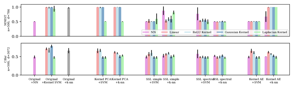
Figure 7: Comparison of kernel methods and neural network models. Plotted is the accuracy for Kernel methods as defined in Section Experiments with the addition of a supervised Neural network on the labelled data as well as the neural network models corresponding to the contrastive and AE kernel methods.

Experimental comparison. Similar to the above comparison we can also define deep learning models analogues to the contrastive SSL models . The general implementation is done in Python with the implementation in PyTorch (Paszke et al. 2019) for fully and optimisation of trained models. The presented setup in Figure 7 is the same as in the main paper with some additional experiments. We firstly extend the analysis by considering SVM as a downstream task as well. We can first note that learning a neural network on the small set of labelled data (most left bar) fails, most likely due to the fact that due to the high complexity of the model overfits the training data. Overall we observe that under SVM the general comparison between neural network and kernel methods are aligned with the one under $k$-nn.

We will conclude this section with some additional remarks on the comparison and connection between Kernel approaches and neural network methods.

Do we need deep kernel representation learning models? Although our construction considers only one a linear functional $\boldsymbol{W}^{\top}\phi({\boldsymbol{x}})$, the feature map $\phi({\boldsymbol{x}})$ can also capture deeper networks. For instance, one may use $L$-layer ReLU NTK (Bietti and Bach 2021) in kernel SSL to model the behaviour “deep” SSL.

Comparison to generalisation error bounds for deep learning models. A common problem in the analysis of modern machine and deep learning methods is that thorough statistical approaches such as VC-dimension (Vapnik 1982, 1998) or Rademacher complexity (Tolstikhin and Lopez-Paz 2016) do not hold in the overparmeterized learning regime. On the other hand in the context of kernel machines those approaches are well developed (Wahba 1990; Schölkopf and Smola 2002; Bartlett and Mendelson 2002a). The proposed extensions allow for a more thorough theoretical analysis of representation learning as well as kernel variants of unsupervised deep learning methods.

Further experiments

In this section we extend the experiments presented in the main section. We additionally provided the performance of linear SVM as a donwstream classifier in addition to the earlier considered $k$-nn classifier. Furthermore we extend the analysis by considering the following datasets.

We denote the split as $split=unlabelled\%/labelled\%/test\%$. We show the results for the following three dadatsets: concentric circles, factor 0.6 $(n=200,d=2,\#classes=2)$ (Pedregosa et al. 2011), cubes $(n=200,d=13,\#classes=4,split=50/10/40)$ (Pedregosa et al. 2011), Iris $(n=150,d=4,\#classes=3,split=50/5/45)$ (Fisher 1936), Ionosphere $(n=351,d=34,\#classes=2,split=50/5/45)$ (Sigillito. et al. 1989), blobs $(n=200,d=2,\#classes=3,split=50/5/45)$ (Pedregosa et al. 2011), Breast cancer $(n=569,d=30,\#classes=2,split=50/5/45)$ (Wolberg et al. 1995), Heart Failure $(n=299,d=13,\#classes=2,split=50/5/45)$ (Davide and Giuseppe 2020), Mushroom (sub-sample) $(n=200,d=22,\#classes=2,split=50/5/45)$ (Schlimmer 1987), Wine $(n=178,d=13,\#classes=3,split=50/10/4)$ (Aeberhard and Forina 1991), Parkinson’s Disease Classification from Speech $(n=756,d=754,\#classes=2,split=50/5/45)$ (Sakar et al. 2019) and Moons $(n=200,d=2,\#classes=2,split=50/5/45)$ (Pedregosa et al. 2011).

We can conclude this section by observing that overall the main findings in the main paper stay consistent throughout the analysis of additional datasets and downstream tasks.

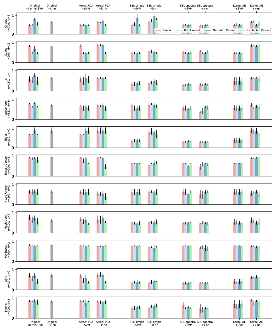
Figure 8: Accuracy for different methods. From left to right: we first consider $k$-nn and Kernel SVM on the original features followed by SVM and $k$-nn on embeddings obtained by Kernel SVM, simple contrastive kernel method, spectral contrastive kernel method and kernel AE.

References

- Aeberhard and Forina (1991) Aeberhard, S.; and Forina, M. 1991. Wine. UCI Machine Learning Repository.
- Aronszajn (1950) Aronszajn, N. 1950. Theory of reproducing kernels. Transactions of the American mathematical society.
- Arora et al. (2019) Arora, S.; Du, S. S.; Hu, W.; Li, Z.; Salakhutdinov, R.; and Wang, R. 2019. On Exact Computation with an Infinitely Wide Neural Net. In Advances in neural information processing systems.
- Bardes, Ponce, and LeCun (2022) Bardes, A.; Ponce, J.; and LeCun, Y. 2022. VICReg: Variance-Invariance-Covariance Regularization for Self-Supervised Learning. In International Conference on Learning Representations.
- Bartlett and Mendelson (2002a) Bartlett, P. L.; and Mendelson, S. 2002a. Rademacher and Gaussian Complexities: Risk Bounds and Structural Results. Journal of Machine Learning Research.
- Bartlett and Mendelson (2002b) Bartlett, P. L.; and Mendelson, S. 2002b. Rademacher and Gaussian complexities: Risk bounds and structural results. Journal of Machine Learning Research.
- Bay, Tuytelaars, and Van Gool (2006) Bay, H.; Tuytelaars, T.; and Van Gool, L. 2006. SURF: Speeded Up Robust Features. In Computer Vision – ECCV 2006. Springer Berlin Heidelberg.
- Bengio, Courville, and Vincent (2013) Bengio, Y.; Courville, A.; and Vincent, P. 2013. Representation learning: A review and new perspectives. IEEE transactions on pattern analysis and machine intelligence.
- Bietti and Bach (2021) Bietti, A.; and Bach, F. 2021. Deep Equals Shallow for ReLU Networks in Kernel Regimes. In International Conference on Learning Representations.
- Bromley et al. (1993) Bromley, J.; Guyon, I.; LeCun, Y.; Säckinger, E.; and Shah, R. 1993. Signature verification using a” siamese” time delay neural network. Advances in neural information processing systems.
- Buades, Coll, and Morel (2005a) Buades, A.; Coll, B.; and Morel, J.-M. 2005a. A review of image denoising algorithms, with a new one. Multiscale modeling & simulation.
- Buades, Coll, and Morel (2005b) Buades, A.; Coll, B.; and Morel, J.-M. 2005b. A review of image denoising algorithms, with a new one. Multiscale Modeling and Simulation: A SIAM Interdisciplinary Journal.
- Carratino, Rudi, and Rosasco (2018) Carratino, L.; Rudi, A.; and Rosasco, L. 2018. Learning with SGD and Random Features. In Advances in Neural Information Processing Systems 31.
- Chahal and Toner (2021) Chahal, H.; and Toner, H. 2021. ‘Small Data’ Are Also Crucial for Machine Learning. Scientific American.
- Chen et al. (2020) Chen, T.; Kornblith, S.; Norouzi, M.; and Hinton, G. 2020. A simple framework for contrastive learning of visual representations. In International conference on machine learning.
- Chen and He (2020) Chen, X.; and He, K. 2020. Exploring Simple Siamese Representation Learning. arXiv preprint arXiv:2011.10566.
- Cortes and Vapnik (1995) Cortes, C.; and Vapnik, V. 1995. Support-vector networks. Machine learning.
- Davide and Giuseppe (2020) Davide, C.; and Giuseppe, J. 2020. Heart failure clinical records. UCI Machine Learning Repository.
- Deng (2012) Deng, L. 2012. The mnist database of handwritten digit images for machine learning research. IEEE Signal Processing Magazine.
- Devlin et al. (2019) Devlin, J.; Chang, M.; Lee, K.; and Toutanova, K. 2019. BERT: Pre-training of Deep Bidirectional Transformers for Language Understanding. In Proceedings of the 2019 Conference of the North American Chapter of the Association for Computational Linguistics: Human Language Technologies,.
- Fernández-Delgado et al. (2014) Fernández-Delgado, M.; Cernadas, E.; Barro, S.; and Amorim, D. 2014. Do we need hundreds of classifiers to solve real world classification problems? The journal of machine learning research.
- Fisher (1936) Fisher, R. A. 1936. The use of multiple measurements in taxonomic problems. Annals of eugenics.
- Ghorbani et al. (2019) Ghorbani, B.; Mei, S.; Misiakiewicz, T.; and Montanari, A. 2019. Limitations of Lazy Training of Two-layers Neural Network. In Advances in Neural Information Processing Systems 32.
- Gretton et al. (2005) Gretton, A.; Bousquet, O.; Smola, A.; and Schölkopf, B. 2005. Measuring statistical dependence with Hilbert-Schmidt norms. In International conference on algorithmic learning theory.
- Grill et al. (2020) Grill, J.-B.; Strub, F.; Altché, F.; Tallec, C.; Richemond, P. H.; Buchatskaya, E.; Doersch, C.; Pires, B. A.; Guo, Z. D.; Azar, M. G.; Piot, B.; Kavukcuoglu, K.; Munos, R.; and Valko, M. 2020. Bootstrap Your Own Latent a New Approach to Self-Supervised Learning. In Advances in neural information processing systems.
- Gu, Kelly, and Xiu (2020) Gu, S.; Kelly, B.; and Xiu, D. 2020. Empirical asset pricing via machine learning. The Review of Financial Studies.
- Hainmueller and Hazlett (2014) Hainmueller, J.; and Hazlett, C. 2014. Kernel regularized least squares: Reducing misspecification bias with a flexible and interpretable machine learning approach. Political Analysis.
- HaoChen et al. (2021) HaoChen, J. Z.; Wei, C.; Gaidon, A.; and Ma, T. 2021. Provable Guarantees for Self-Supervised Deep Learning with Spectral Contrastive Loss. In Advances in neural information processing systems.
- Jacot, Gabriel, and Hongler (2018) Jacot, A.; Gabriel, F.; and Hongler, C. 2018. Neural Tangent Kernel: Convergence and Generalization in Neural Networks. In Advances in neural information processing systems.
- Jing and Tian (2019) Jing, L.; and Tian, Y. 2019. Self-Supervised Visual Feature Learning With Deep Neural Networks: A Survey. IEEE Transactions on Pattern Analysis and Machine Intelligence.
- Johnson, Hanchi, and Maddison (2022) Johnson, D. D.; Hanchi, A. E.; and Maddison, C. J. 2022. Contrastive Learning Can Find An Optimal Basis For Approximately View-Invariant Functions. arXiv preprint arXiv:2210.01883.
- Kanazawa, Jacobs, and Chandraker (2016) Kanazawa, A.; Jacobs, D. W.; and Chandraker, M. 2016. Warpnet: Weakly supervised matching for single-view reconstruction. In IEEE Conference on Computer Vision and Pattern Recognition.
- Kiani et al. (2022) Kiani, B. T.; Balestriero, R.; Chen, Y.; Lloyd, S.; and LeCun, Y. 2022. Joint embedding self-supervised learning in the kernel regime. arXiv preprint arXiv:2209.14884.
- Kimeldorf and Wahba (1971) Kimeldorf, G.; and Wahba, G. 1971. Some results on Tchebycheffian spline functions. Journal of Mathematical Analysis and Applications.
- Kramer (1991) Kramer, M. A. 1991. Nonlinear principal component analysis using autoassociative neural networks. AIChE journal.
- Krizhevsky, Hinton et al. (2009) Krizhevsky, A.; Hinton, G.; et al. 2009. Learning multiple layers of features from tiny images.
- Kunin et al. (2019) Kunin, D.; Bloom, J.; Goeva, A.; and Seed, C. 2019. Loss Landscapes of Regularized Linear Autoencoders. In International Conference on Machine Learning.
- Liu, Zhu, and Belkin (2020) Liu, C.; Zhu, L.; and Belkin, M. 2020. On the linearity of large non-linear models: when and why the tangent kernel is constant. In Advances in Neural Information Processing Systems 33.
- Lowe (1999) Lowe, D. G. 1999. Object recognition from local scale-invariant features. In Proceedings of the seventh IEEE international conference on computer vision.
- Maurer (2016) Maurer, A. 2016. A Vector-Contraction Inequality for Rademacher Complexities. In Ortner, R.; Simon, H. U.; and Zilles, S., eds., Algorithmic Learning Theory. Springer International Publishing.
- Maurer and Pontil (2016) Maurer, A.; and Pontil, M. 2016. Bounds for vector-valued function estimation. arXiv preprint arXiv:1606.01487.
- Mika et al. (1999) Mika, S.; Ratsch, G.; Weston, J.; Scholkopf, B.; and Mullers, K.-R. 1999. Fisher discriminant analysis with kernels. In Neural networks for signal processing IX: Proceedings of the 1999 IEEE signal processing society workshop.
- Misra and Maaten (2020) Misra, I.; and Maaten, L. v. d. 2020. Self-supervised learning of pretext-invariant representations. In Proceedings of the IEEE/CVF Conference on Computer Vision and Pattern Recognition.
- Netzer et al. (2011) Netzer, Y.; Wang, T.; Coates, A.; Bissacco, A.; Wu, B.; and Ng, A. Y. 2011. Reading Digits in Natural Images with Unsupervised Feature Learning. In NIPS Workshop on Deep Learning and Unsupervised Feature Learning 2011.
- Nguyen, Wong, and Hegde (2021) Nguyen, T. V.; Wong, R. K. W.; and Hegde, C. 2021. Benefits of Jointly Training Autoencoders: An Improved Neural Tangent Kernel Analysis. IEEE Transactions on Information Theory.
- Paszke et al. (2019) Paszke, A.; Gross, S.; Massa, F.; Lerer, A.; Bradbury, J.; Chanan, G.; Killeen, T.; Lin, Z.; Gimelshein, N.; Antiga, L.; Desmaison, A.; Kopf, A.; Yang, E.; DeVito, Z.; Raison, M.; Tejani, A.; Chilamkurthy, S.; Steiner, B.; Fang, L.; Bai, J.; and Chintala, S. 2019. PyTorch: An Imperative Style, High-Performance Deep Learning Library. In Advances in Neural Information Processing Systems.
- Pearson (1901) Pearson, K. 1901. On lines and planes of closest fit to systems of points in space. The London, Edinburgh, and Dublin Philosophical Magazine and Journal of Science.
- Pedregosa et al. (2011) Pedregosa, F.; Varoquaux, G.; Gramfort, A.; Michel, V.; Thirion, B.; Grisel, O.; Blondel, M.; Prettenhofer, P.; Weiss, R.; Dubourg, V.; Vanderplas, J.; Passos, A.; Cournapeau, D.; Brucher, M.; Perrot, M.; and Duchesnay, E. 2011. Scikit-learn: Machine Learning in Python. Journal of Machine Learning Research.
- Ponte and Melko (2017) Ponte, P.; and Melko, R. G. 2017. Kernel methods for interpretable machine learning of order parameters. Physical Review B.
- Pretorius, Kroon, and Kamper (2018) Pretorius, A.; Kroon, S.; and Kamper, H. 2018. Learning Dynamics of Linear Denoising Autoencoders. In International Conference on Machine Learning.
- Radhakrishnan, Belkin, and Uhler (2020) Radhakrishnan, A.; Belkin, M.; and Uhler, C. 2020. Overparameterized neural networks implement associative memory. Proceedings of the National Academy of Sciences of the United States of America.
- Rahimi and Recht (2007) Rahimi, A.; and Recht, B. 2007. Random Features for Large-Scale Kernel Machines. In Advances in Neural Information Processing Systems 20.
- Refinetti and Goldt (2022) Refinetti, M.; and Goldt, S. 2022. The dynamics of representation learning in shallow, non-linear autoencoders. In International Conference on Machine Learning.
- Roßbach (2018) Roßbach, P. 2018. Neural networks vs. random forests–does it always have to be deep learning.
- Sakar et al. (2019) Sakar, C. O.; Serbes, G.; Gunduz, A.; Tunc, H. C.; Nizam, H.; Sakar, B. E.; Tutuncu, M.; Aydin, T.; Isenkul, M. E.; and Apaydin, H. 2019. A comparative analysis of speech signal processing algorithms for Parkinson’s disease classification and the use of the tunable Q-factor wavelet transform. Applied Soft Computing.
- Saunshi et al. (2019) Saunshi, N.; Plevrakis, O.; Arora, S.; Khodak, M.; and Khandeparkar, H. 2019. A Theoretical Analysis of Contrastive Unsupervised Representation Learning. In Proceedings of the 36th International Conference on Machine Learning.
- Schlimmer (1987) Schlimmer, J. 1987. Mushroom. UCI Machine Learning Repository.
- Schölkopf, Herbrich, and Smola (2001) Schölkopf, B.; Herbrich, R.; and Smola, A. J. 2001. A Generalized Representer Theorem. In Annual Conference on Computational Learning Theory.
- Schölkopf and Smola (2002) Schölkopf, B.; and Smola, A. J. 2002. Learning with Kernels: support vector machines, regularization, optimization, and beyond. Adaptive computation and machine learning series. MIT Press.
- Schölkopf, Smola, and Müller (1998) Schölkopf, B.; Smola, A.; and Müller, K.-R. 1998. Nonlinear Component Analysis as a Kernel Eigenvalue Problem. Neural Computation.
- Shah et al. (2022) Shah, A.; Sra, S.; Chellappa, R.; and Cherian, A. 2022. Max-Margin Contrastive Learning. In Proceedings of the AAAI Conference on Artificial Intelligence.
- Shwartz-Ziv and Armon (2022) Shwartz-Ziv, R.; and Armon, A. 2022. Tabular data: Deep learning is not all you need. Inf. Fusion.
- Sigillito. et al. (1989) Sigillito., V.; S., W.; L., H.; ; and K., B. 1989. Ionosphere. UCI Machine Learning Repository. DOI: https://doi.org/10.24432/C5W01B.
- Todman, Bush, and Hood (2023) Todman, L. C.; Bush, A.; and Hood, A. S. 2023. ‘Small Data’for big insights in ecology. Trends in Ecology & Evolution.
- Tolstikhin and Lopez-Paz (2016) Tolstikhin, I. O.; and Lopez-Paz, D. 2016. Minimax Lower Bounds for Realizable Transductive Classification. In ArXiv, volume 1602.03027.
- Vapnik (1982) Vapnik, V. 1982. Estimation of Dependences Based on Empirical Data. In Springer Series in Statistics.
- Vapnik (1998) Vapnik, V. 1998. Statistical Learning Theory. In A Wiley-Interscience publication.
- Vincent et al. (2010) Vincent, P.; Larochelle, H.; Lajoie, I.; Bengio, Y.; Manzagol, P.-A.; and Bottou, L. 2010. Stacked denoising autoencoders: Learning useful representations in a deep network with a local denoising criterion. Journal of machine learning research.
- Wahba (1990) Wahba, G. 1990. Spline Models for Observational Data. SIAM.
- Wolberg et al. (1995) Wolberg, W.; Mangasarian, O.; Street, N.; and Street, W. 1995. Breast Cancer Wisconsin (Diagnostic). UCI Machine Learning Repository.
- Xu et al. (2023) Xu, P.; Ji, X.; Li, M.; and Lu, W. 2023. Small data machine learning in materials science. npj Computational Materials.
- Yang et al. (2017) Yang, B.; Fu, X.; Sidiropoulos, N. D.; and Hong, M. 2017. Towards k-means-friendly spaces: Simultaneous deep learning and clustering. In international conference on machine learning, 3861–3870. PMLR.
- Zhai et al. (2023) Zhai, R.; Liu, B.; Risteski, A.; Kolter, Z.; and Ravikumar, P. 2023. Understanding Augmentation-based Self-Supervised Representation Learning via RKHS Approximation. arXiv preprint arXiv:2306.00788.
- Zhang et al. (2022) Zhang, C.; Zhang, C.; Song, J.; Yi, J. S. K.; Zhang, K.; and Kweon, I. S. 2022. A survey on masked autoencoder for self-supervised learning in vision and beyond. arXiv preprint arXiv:2208.00173.