Granger Causal Inference in Multivariate Hawkes Processes by Minimum Message Length

Abstract

Multivariate Hawkes processes (MHPs) are versatile probabilistic tools used to model various real-life phenomena: earthquakes, operations on stock markets, neuronal activity, virus propagation and many others. In this paper, we focus on MHPs with exponential decay kernels and estimate connectivity graphs, which represent the Granger causal relations between their components. We approach this inference problem by proposing an optimization criterion and model selection algorithm based on the minimum message length (MML) principle. MML compares Granger causal models using the Occam’s razor principle in the following way: even when models have a comparable goodness-of-fit to the observed data, the one generating the most concise explanation of the data is preferred. While most of the state-of-art methods using lasso-type penalization tend to overfitting in scenarios with short time horizons, the proposed MML-based method achieves high F1 scores in these settings. We conduct a numerical study comparing the proposed algorithm to other related classical and state-of-art methods, where we achieve the highest F1 scores in specific sparse graph settings. We illustrate the proposed method also on G7 sovereign bond data and obtain causal connections, which are in agreement with the expert knowledge available in the literature.

Keywords: Granger causal inference, multivariate Hawkes processes, minimum message length, model selection and parameter estimation

1 Introduction

Many practical applications deal with a large amount of irregular and asynchronous sequential data observed within a fixed time horizon. One can interpret such data as event sequences containing stereotypic events, which can be modeled via multidimensional point processes. These events can be, e.g. user viewing records, patient records in hospitals (in which times, diagnoses or treatments are provided), various levels of earthquakes, high-frequency financial transactions or neuronal activity.

In this paper, we focus on a special type of point processes, known as Hawkes processes (Hawkes, 1971). Their main advantage over other point processes (such as the classical Poisson processes) is that they permit to model the influence of past events, thanks to their “memory” property, as well as possible interactions between different components of the process. In particular, we consider multivariate Hawkes processes (MHPs) of the type ${\boldsymbol{X}}=({\boldsymbol{X}}_{t})_{t\in[0,T]}=(X^{1}_{t},\dots,X^{p}_{t})_{t\in[0,T]}$, $T>0$, which represent a system of $p\geq 2$ interacting units. The value $T$ is called the time horizon of a MHP. The case when $T$ is of order at most a hundred times the dimension $p$ is referred to as a “short” time horizon. If $T$ is of order at least a thousands times the dimension $p$, we talk about a “long” time horizon. One can interpret each component of a MHP as a “particle” or “node” in some given system, e.g. a neuron in a brain, an account in a social network, or a certain type of financial transaction. A realization (path) of the process corresponds to a list of events (or “jumps”) which occur within the time interval $[0,T]$. In particular, for each $i\in\{1,\ldots,p\}$, the vector of observed events of the $i$-th particle $(X^{i}_{t})_{t\in[0,T]}$ is given by $\boldsymbol{x}_{i}=(t^{i}_{1},\dots,t^{i}_{n_{i}})^{\top}$, where $n_{i}\in\mathbb{N}$ and $0<t^{i}_{1}<\dots<t^{i}_{n_{i}}\leq T$, and a realization of the entire process $\boldsymbol{X}$ is given by $\boldsymbol{x}=\{\boldsymbol{x}_{i}\}_{i=1}^{p}$. Moreover, each component $(X^{i}_{t})_{t\in[0,T]}$ of a MHP is defined by its conditional intensity:

$$\mathbb{P}\left(X^{i}\text{ has a jump in }[t,t+dt]|\mathcal{F}_{t}\right)=\lambda_{i}(t)dt,$$ (1)

where $\mathcal{F}_{t}$ is a history of events occurring before time $t$, and

$$\lambda_{i}(t)=\mu_{i}+\sum_{j=1}^{p}\int_{0}^{t}\alpha_{ij}\exp(-\beta_{ij}(t-\tau))dX^{j}_{\tau},$$ (2)

where the $\mu_{i}>0$ are positive parameters also known as background intensities, $\beta_{ij}>0$ are positive decay constants, and $\alpha_{ij}\geq 0$ are non-negative influence parameters, which model the interaction between different components of the process $\boldsymbol{X}$. Since we focus on interaction functions given by an exponential kernel, we will refer to $\boldsymbol{X}$ as exp-MHP.

The main objective of this paper is to infer the connectivity graph, which describes the Granger-causal relationships between the components of exp-MHPs. We use the notion of Granger causality among Hawkes processes based on the definition from Eichler et al. (2017) and say that the component $X^{j}$ does not Granger-cause $X^{i}$ if and only if the corresponding interaction function is equal to $0$ for all $t\in[0,T]$. Since our interaction function is given by $\alpha_{ij}\exp(-\beta_{ij}(t-\tau))$ this holds if and only if the influence parameter $\alpha_{ij}=0$. In this case, there is no edge leading from $j$ to $i$ in the corresponding graph, otherwise an edge $j\to i$ is present in the graph. In other words, we study the problem of estimating the connections in a directed graph when the underlying model is an exp-MHP.

We approach this inference problem by proposing a model selection algorithm called MMLH for exp-MHPs based on the so called minimum message length (MML) principle, originally proposed in Wallace and Boulton (1968). Methods using MML learn through a data compression perspective and are sometimes described as mathematical applications of Occam’s razor, see e.g. Grünwald and Roos (2019).

As the proposed MMLH algorithm to recover causal connections in exp-MHPs is a model selection method, it allows to incorporate possible expert knowledge about the underlying structure. Parametric inference methods on the contrary, e.g. maximum-likelihood estimation (MLE), require all parameters to be estimated simultaneously, which can result in a poor performance. In contrast to other model selection methods, such as the classical one obtained via the Bayesian information criterion (BIC) or the recent method proposed by Jalaldoust et al. (2022) based on the data compression technique “minimum description length” (MDL), MMLH incorporates prior distributions of relevant model parameters, making the method more flexible in terms of structure-related penalty.

We compare the proposed MMLH algorithm to two state-of-the-art methods (the related MDL-based method from Jalaldoust et al. (2022) and the method ADM4 from Zhou et al. (2013)), as well as to two standard reference methods, namely BIC and MLE. We focus on data with short time horizons and consider graphs of dimension seven, ten, and twenty, respectively. MMLH shows the highest F1 accuracy with respect to all considered methods for specific sparse graph settings. We complete the numerical study by applying our approach on a real-world data base, which describes the return volatility of sovereign bonds of seven large economies (see e.g. Demirer et al. (2018); Jalaldoust et al. (2022)). Most discovered causal connections are in accordance with the expert knowledge from the literature.

Notations.

Regarding terminology, we use both terms “causal structure” and “connectivity graph”, depending on which is more appropriate in the respective context. Regarding notation, scalar variables are denoted by regular letters and vectors and matrices by bold letters. Stochastic processes are denoted by capital letters (e.g. $\boldsymbol{X}$) and any realization or point by a lower-case letter (e.g. ${\boldsymbol{x}}$). Matrices are denoted by Greek or capital regular letters. Let $\boldsymbol{\alpha}$ be a generic matrix. Then $\boldsymbol{\alpha}_{i}$ denotes the $i$-th row of the matrix $\boldsymbol{\alpha}$ and $\alpha_{ij}$ the $j$-th entry in the $i$-th row. Moreover, $\boldsymbol{\alpha}^{\top}$ and $|\boldsymbol{\alpha}|$ denote the transpose and determinant of the matrix $\boldsymbol{\alpha}$, respectively.

This paper is organized as follows. Section 2 discusses related work. Section 3 recalls the general idea of MML as a criterion for model selection and parameter estimation. In Section 4, we apply the MML approach to exp-MHPs. The proposed algorithm MMLH is described in Section 5. In Section  6, we illustrate the performance of the proposed algorithm in comparison to benchmark methods on both synthetic data as well as real-world data. Section 7 concludes the study and outlines perspectives for possible future work. A sample code is available at: https://github.com/IreneTubikanec/MMLH

2 Related Work

Related work can be categorized into the work on discovery of Granger causal networks in MHPs and on applying compression based methods (such as MML and MDL) to Granger causal inference.

The problem of inferring the Granger causal structure is relatively new in the context of MHPs, however, it has attracted a lot of attention in recent years, see e.g. Hansen et al. (2015), Xu et al. (2016) and Sulem et al. (2021). Didelez (2008) studied causal connectivity graphs for discrete time events and extended them to marked point processes. Most of the related work deals with variable selection in sparse causal graphs. The recovery of the Granger causal structure is directly linked to the problem of (parametric or nonparametric) estimation of the interaction function, which is studied in the literature, e.g. by Eichler et al. (2017). The most common approach to reconstruct the network is to apply maximum likelihood estimation, see e.g. Ogata (1988), Veen and Schoenberg (2008), Juditsky et al. (2020). Maximum likelihood estimation reveals favorable theoretical properties and is not computationally expensive. However, it does not lead to good scores in practice, especially on small datasets. Some improvement can be achieved when the estimation is done via confidence intervals (as in Wang et al. (2020)), however, they are difficult to compute for a general class of models. Xu et al. (2016) applied an expectation maximization (EM) algorithm based on a penalized likelihood objective leading to temporal and group sparsity to infer a Granger graph in MHPs.

The method ADM4 in Zhou et al. (2013) performs variable selection by using lasso and nuclear norm regularization simultaneously on the parameters to cluster variables as well as to obtain a sparse connectivity graph. The method NPHC (Achab et al. 2017) takes a non-parametric approach in learning the norm of the kernel functions to find the causal connectivity graph. The method uses a moment-matching approach to fit the second-order and third-order integrated cumulants of the process.

To infer a causal connectivity graph, Bacry et al. (2020) optimize a least-square based objective function with lasso and trace norm of the interaction tensor for the intensity process. Trouleau et al. (2021) investigated stability of cumulant-based estimators for causal inference in MHPs with respect to noise. Wei et al. (2023) recover a Granger causal graph for Hawkes processes coupled with the so-called ReLU link function; It was tested on long time horizons $T$ and, in comparison to other mentioned methods, it considers both exciting and inhibiting effects. Idé et al. (2021) introduced a causal learning framework based on a cardinality-regularized Hawkes process. Hansen et al. (2015) use lasso penalization to infer sparse connectivity graphs in MHPs. Most of the above mentioned methods using lasso-type penalization demonstrated good performance in scenarios with long time horizons $T$. It is however known that lasso-type penalization methods often suffer from overfitting in the opposite case of short time horizons, see e.g. Reid et al. (2016). To overcome the drawbacks of these methods, we approach penalization based on the MML principle.

MML-based model selection as an inductive inference method based on data compression was first introduced in Wallace and Boulton (1968). Intuitively, the recovery of a connectivity graph using the MML principle is equivalent to selecting an optimal model for the observed data, where “optimal” means “the one which permits to encode the data in a binary string of the shortest length” in terms of coding theory. There exist papers on the recovery of Granger connectivity graphs by MML for processes having distributions from exponential families, see Hlaváčková-Schindler and Plant (2020a, b), but to the best of our knowledge, not for MHPs. Another compression scheme using Occam’s razor in terms of coding representations is the minimum description length (Rissanen (1998)), which was more recently developed in Grünwald (2007) and Grünwald and Roos (2019). In comparison to MML, the MDL principle does not use any knowledge of priors. MDL-based Granger-causal inference has been recently applied to exp-MHPs in Jalaldoust et al. (2022) and to Gaussian processes in Hlaváčková-Schindler and Plant (2020b).

3 Minimum Message Length Criterion and Its Approximation

Methods based on the MML principle consider the model which compresses the data the most (i.e., the one with the “shortest message length”). To be able to decompress this representation of the data, the details of the statistical model used to encode the data must also be a part of the compressed data string. The calculation of the exact message is an NP-hard problem, since it corresponds to the Kolmogorov complexity (see Wallace and Dowe (1999)), which is in general not computable due to the halting problem (see Li and Vitányi (2008)). However, there exist computable approximations of MML, the most used one is the Wallace–Freeman approximation (Wallace and Freeman, 1987), which we will use in this paper (see Section 3.2).

Before we recall the general idea behind MML and outline the aforementioned approximation approach, we define statistical models. Statistical models are families of probability distributions of the form

$$M=\{p(\cdot|\boldsymbol{\theta}):\boldsymbol{\theta}\in\boldsymbol{\Theta}\},$$ (3)

parameterized by a set $\boldsymbol{\Theta}$ (usually a subset of a Euclidean space). They are represented by families of probability distributions

$$\{M_{\boldsymbol{\gamma}}:\boldsymbol{\gamma}\in\boldsymbol{\Gamma}\},$$ (4)

where $\boldsymbol{\Gamma}$ is a countable set of so-called “structures” and, for each structure $\boldsymbol{\gamma}\in\boldsymbol{\Gamma}$,

$$M_{\boldsymbol{\gamma}}=\{p_{\boldsymbol{\gamma}}(\cdot|\boldsymbol{\theta}):\boldsymbol{\theta}\in\boldsymbol{\Theta}_{\boldsymbol{\gamma}}\}$$ (5)

is a statistical model, parameterized by the space $\boldsymbol{\Theta}_{\boldsymbol{\gamma}}$.

In our setting, the set of structures $\boldsymbol{\Gamma}$ can be interpreted as a countable set of binary vectors, i.e. $\boldsymbol{\Gamma}=\{0,1\}^{q}$ with $q>0$. Each element $\boldsymbol{\gamma}\in\boldsymbol{\Gamma}$ is then a $q$-dimensional vector of zeros and ones, where the number of ones is given by $k$, and where $\gamma_{j}=1$ denotes the presence of the $j$-th variable in the subset of $k$ variables, and $\gamma_{j}=0$ means that the $j$-th variable is not present. The parameters $\boldsymbol{\theta}\in\boldsymbol{\Theta}_{\boldsymbol{\gamma}}\subset\mathbb{R}^{k}$ then define the ”weights” (which can be interpreted as importance measures) with respect to the variables in $\boldsymbol{\gamma}$.

3.1 Idea Behind the Minimum Message Length Method

The MML principle is a formal information theory restatement of Occam’s razor: even when models have a comparable goodness-of-fit to the observed data, the one generating the shortest overall message is more likely to be correct (where the message consists of a statement of the model, followed by a statement of data encoded concisely using that model). Let us describe the idea of the MML method more formally.

Consider some data $\boldsymbol{y}=(y_{1},\dots,y_{n})^{\top}\in\mathbb{R}^{n}$ that we would like to send to a receiver by encoding it into a message (e.g. a binary string). The key idea in MML inference is to interpret this message as consisting of two parts: an ecoding (called assertion) of the model and associated parameters $\boldsymbol{\theta}\in\boldsymbol{\Theta}$, and a description (called detail) of the data $\boldsymbol{y}$ using the model $p({\boldsymbol{y}}|\boldsymbol{\theta})$ specified in the assertion. The total message length of the data $\boldsymbol{y}$ and model parameterization $\boldsymbol{\theta}\in\boldsymbol{\Theta}$ is then given by

$$I({\boldsymbol{y}};\boldsymbol{\theta})=I(\boldsymbol{\theta})+I({\boldsymbol{y}}|\boldsymbol{\theta}),$$ (6)

where $I(\boldsymbol{\theta})$ and $I({\boldsymbol{y}}|\boldsymbol{\theta})$ denote the length of the assertion and detail, respectively. The length of the assertion $I(\boldsymbol{\theta})$ is a measure of the model complexity, while the length of the detail $I({\boldsymbol{y}}|\boldsymbol{\theta})$ is a measure of the goodness-of-fit of the model to the data (model capability). MML seeks the model that minimizes this trade off between model complexity and model capability, i.e.

$$\hat{\boldsymbol{\theta}}=\textrm{argmin}_{\boldsymbol{\theta}\in\boldsymbol{\Theta}}\ I({\boldsymbol{y}};\boldsymbol{\theta}).$$ (7)

In the type of MML considered here, the parameter space $\boldsymbol{\Theta}$ for the statistical model $p(.|\boldsymbol{\theta})$ is decomposed into a countable number of subsets and associated code words for members of these subsets, i.e. $\boldsymbol{\Theta}=\cup_{\boldsymbol{\gamma}\in\boldsymbol{\Gamma}}\boldsymbol{\Theta}_{\boldsymbol{\gamma}}$. The code of the structure $\boldsymbol{\gamma}\in\boldsymbol{\Gamma}$ is then included into the total message length (6). In particular, the refined total message length of data ${\boldsymbol{y}}\in\mathbb{R}^{n}$ and model parameterization $\boldsymbol{\theta}\in\boldsymbol{\Theta}_{\boldsymbol{\gamma}}$ including the structure of parameters is given by

$$I({\boldsymbol{y}};\boldsymbol{\theta};\boldsymbol{\gamma})=I(\boldsymbol{\gamma})+I(\boldsymbol{\theta};\boldsymbol{\gamma})+I({\boldsymbol{y}}|\boldsymbol{\theta};\boldsymbol{\gamma}),$$ (8)

where, for $\gamma\in\boldsymbol{\Gamma}=\{0,1\}^{q}$, the set of all possible structures, we set

$$I(\boldsymbol{\gamma})=\log\dbinom{q}{k}+\log(q+1),$$ (9)

as recommended by Roos et al. (2009). Note that in this refined MML setup, the coding scheme (i.e. the set $\boldsymbol{\Theta}_{\boldsymbol{\gamma}}$ and corresponding code words) is agreed upon by both the sender and receiver before any data is seen. As before, MML seeks the model that minimizes this trade off between the model complexity and model capability, i.e.

$$\{\hat{\boldsymbol{\gamma}},\hat{\boldsymbol{\theta}}\}=\textrm{argmin}_{\boldsymbol{\gamma}\in\boldsymbol{\Gamma},\boldsymbol{\theta}\in\boldsymbol{\Theta}_{\boldsymbol{\gamma}}}\ I({\boldsymbol{y}};\boldsymbol{\theta};\boldsymbol{\gamma}).$$ (10)

3.2 Wallace-Freeman 1987 Approximation

In the following, we recall a well-known approximation of the total message length introduced in (8). As proposed in Wallace and Freeman (1987), the codelength of data $\boldsymbol{y}$ for a given model parameterization $\boldsymbol{\theta}\in\boldsymbol{\Theta}_{\boldsymbol{\gamma}}$ under a fixed structure $\gamma\in\boldsymbol{\Gamma}=\{0,1\}^{q}$ (i.e., the detail w.r.t. $\gamma$) is given by

$$I({\boldsymbol{y}}|\boldsymbol{\theta};\boldsymbol{\gamma})\approx-\log p_{\boldsymbol{\gamma}}({\boldsymbol{y}}|\boldsymbol{\theta})+\frac{k}{2}.$$ (11)

Moreover, the codelength of the assertion w.r.t. $\gamma$ is given by

$$I(\boldsymbol{\theta};\gamma)\approx-\log\pi_{\boldsymbol{\gamma}}(\boldsymbol{\theta})+\frac{1}{2}\log|J_{\boldsymbol{\gamma}}(\boldsymbol{\theta})|+\frac{k}{2}\log\kappa_{k},$$ (12)

where $\pi_{\boldsymbol{\gamma}}(\boldsymbol{\theta})$ is a prior probability distribution over $\boldsymbol{\Theta}_{\gamma}$, making the procedure Bayesian, $J_{\gamma}(\boldsymbol{\theta})$ is the expected Fisher information matrix and $\kappa_{k}$ is a quantizing lattice constant, which depends on the number of parameters $k$ that is determined by the structure $\gamma$.

While an optimal value for $\kappa_{k}$ is not available in general, in Wallace and Freeman (1987) the following upper and lower bounds were proposed for $k>1$:

$$\frac{\Gamma(k/2+1)^{2/k}}{\pi(k+2)}<\kappa_{k}<\frac{\Gamma(k/2+1)^{2/k}\Gamma(2/k+1)}{\pi k},$$ (13)

where in this case $\Gamma$ denotes the gamma function. These bounds are reported as function of $k$ (black solid lines) in Figure 1. They both converge to $1/(2\pi e)$ (red dashed line) for $k\to\infty$. Some values of $\kappa_{k}$ (for small $k$) are known explicitly, see e.g. Conway and Sloane (1984), Makalic and Schmidt (2021). Those reported in Table 1 of Conway and Sloane (1984) are added as grey dots to Figure 1. For $k=1$, it is known that $\kappa_{k}=1/12$, and thus the lower bound in (13) is achieved, see Makalic and Schmidt (2021). The choice of approximation for $\kappa_{k}$ influences the penalty term with respect to the number of parameters $k$ determined by the structure $\gamma$.

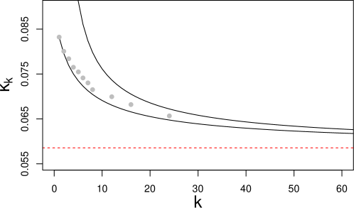
Figure 1: Black solid lines: Upper and lower bounds for $\kappa_{k}$. Red dashed line: Limit of the bounds for $k\to\infty$. Grey dots: Known values of $\kappa_{k}$.

We focus on the approximation

$$\frac{k}{2}(\log\kappa_{k}+1)\approx-\frac{k}{2}\log(2\pi)+\frac{1}{2}\log(k\pi)+\psi(1),$$ (14)

proposed by Wallace (2005), where $\psi$ denotes the digamma function and $\psi(1)\approx-0.5772$.

Using (9) and the approximations (11), (12) and (14), the total message length (8) can be approximated as follows:

$$I(\boldsymbol{y};\boldsymbol{\theta};\boldsymbol{\gamma})\approx -\log p_{\boldsymbol{\gamma}}({\boldsymbol{y}}|\boldsymbol{\theta})-\log\pi_{\boldsymbol{\gamma}}(\boldsymbol{\theta})+\frac{1}{2}\log|J_{\boldsymbol{\gamma}}(\boldsymbol{\theta})|$$ (15)

$$-\frac{k}{2}\log(2\pi)+\frac{1}{2}\log(k\pi)+\psi(1)$$

$$+\log\dbinom{q}{k}+\log(q+1).$$

4 Causal Structure Recovery in Multivariate Hawkes Processes by Minimum Message Length

In this section, we present the proposed MML-based procedure for causal inference in exp-MHPs defined via intensity (2). First, we define the corresponding parameter space $\boldsymbol{\Theta}$. Second, we introduce the components required to define the total message length (15) for exp-MHPs over the parameter space $\boldsymbol{\Theta}$. In particular, we report an explicit expression of the the log-likelihood, derive an approximation for the Fisher information matrix, and choose appropriate prior distributions. Finally, we introduce suitable structures, include them in the aforementioned expressions, and propose a criterion for the total message length in exp-MHPs.

4.1 Parameter Space for Exp-MHPs

Consider an exp-MHP $\boldsymbol{X}$, i.e. a MHP defined via intensity (2). Throughout, we assume for all $i,j\in\{1,\ldots,p\}$ that the decay constants $\beta_{ij}$ are known, and that the background intensities $\mu_{i}$ of the $i$-th particle $X^{i}$ and the influence vector $\mathbf{\boldsymbol{\alpha}}_{i}=(\alpha_{i1},\dots,\alpha_{ip})^{\top}$ on $X^{i}$ are not known. Considering the entire process $\boldsymbol{X}$, we also introduce the unknown baseline vector $\boldsymbol{\mu}=(\mu_{1},\ldots,\mu_{p})^{\top}$ and influence matrix $\boldsymbol{\alpha}$, whose $i$-th row corresponds to the influence vector $\boldsymbol{\alpha}_{i}$. The parameter vector of $\boldsymbol{X}$ is then defined as

$$\boldsymbol{\theta}=[\boldsymbol{\theta}_{1}^{\top},\boldsymbol{\theta}_{2}^{\top},\dots,\boldsymbol{\theta}_{p}^{\top}]^{\top}\in\boldsymbol{\Theta}=(\mathbb{R}^{+}_{0})^{p+p^{2}},$$ (16)

where

$$\boldsymbol{\theta}_{i}=(\mu_{i},\boldsymbol{\alpha}_{i}^{\top})^{\top}\in\boldsymbol{\Theta}_{i}=(\mathbb{R}^{+}_{0})^{p+1}$$ (17)

is the parameter vector of the $i$-th component $X^{i}$, for $i\in\{1,\ldots,p\}$.

4.2 Log-Likelihood for Exp-MHPs

In the following, we recall the log-likelihood of an exp-MHP, see, e.g. Ozaki (1979) (univariate case) and Shlomovich et al. (2022) (multivariate case). Consider an observation $\boldsymbol{x}$ of an exp-MHP $\boldsymbol{X}$ and the parameter vector $\boldsymbol{\theta}\in\boldsymbol{\Theta}$ (16). Then, the log-likelihood can be decomposed as

$$\log p(\boldsymbol{x}|\boldsymbol{\theta})=-\sum_{i=1}^{p}\left(\int_{0}^{T}\lambda_{i}(s)ds-\sum_{j=0}^{n_{i}}\log\lambda_{i}(t^{i}_{j})\right).$$ (18)

Since each summand of this function depends only on the $i$-th dimension $\boldsymbol{\theta}_{i}$ (17) of the parameter vector $\boldsymbol{\theta}$ (16), the negative log-likelihood function can be written as the following sum:

$$-\log p(\boldsymbol{x}|\boldsymbol{\theta})=-\sum_{i=1}^{p}\log p_{i}(\boldsymbol{x}|\boldsymbol{\theta}_{i}),$$ (19)

where each summand represents the marginal negative log-likelihood of the corresponding node. To ease the notations, define $l(\boldsymbol{x}|\boldsymbol{\theta}):=-\log p(\boldsymbol{x}|\boldsymbol{\theta})$ and $l_{i}(\boldsymbol{x}|\boldsymbol{\theta}_{i}):=-\log p_{i}(\boldsymbol{x}|\boldsymbol{\theta}_{i})$. The explicit expression for each $l_{i}(\boldsymbol{x}|\boldsymbol{\theta}_{i})$ can be derived using (2) and is given by

$$l_{i}(\boldsymbol{x}|\boldsymbol{\theta}_{i})=\mu_{i}t^{\max}+\sum_{j=1}^{p}\frac{\alpha_{ij}}{\beta_{ij}}\sum_{k=1}^{n_{j}}\left[1-\exp(-\beta_{ij}(t^{\max}-t^{j}_{k}))\right]\\ -\sum_{l=1}^{n_{i}}\log\left[\mu_{i}+\sum_{j=1}^{p}\alpha_{ij}\sum_{k:t^{j}_{k}<t^{i}_{l}}\exp(-\beta_{ij}(t^{i}_{l}-t^{j}_{k}))\right],$$ (20)

where $t^{\max}\leq T$ is the largest jump time recorded over all nodes.

Remark 1

The function $l_{i}(\boldsymbol{x}|\boldsymbol{\theta}_{i})$ from (20) is convex in $\boldsymbol{\alpha}_{i}$ and $\mu_{i}$. Thus, the maximum likelihood estimate (MLE) can be computed using convex optimization. The proof of convexity can be found, e.g. in Ogata (1981).

4.3 Hessian Matrix for Exp-MHPs

In this section, we derive an explicit expression for the Hessian matrix $H(\boldsymbol{\theta})$ of the negative log-likelihood $l(\boldsymbol{x}|\boldsymbol{\theta})$ based on formula (20), see Shlomovich et al. (2022). Note that the Fisher information matrix $J$, required in the total message length criterion (15), is defined as the expected Hessian. In general, this expectation is difficult to compute and it is often replaced by the observed Fisher information. The observed Fisher information, in turn, is given by the Hessian, evaluated at an estimate $\hat{\boldsymbol{\theta}}$ of $\boldsymbol{\theta}$.

To obtain the Hessian, we first need to compute the gradient of the negative log-likelihood $l(\boldsymbol{x}|\boldsymbol{\theta})$. The required first-order derivatives can be computed explicitly and are given by

$$\frac{\partial l(\boldsymbol{x}|\boldsymbol{\theta})}{\partial\mu_{i}} =t^{\max}-\sum_{l=1}^{n_{i}}\frac{1}{\mu_{i}+\sum_{k=1}^{p}\alpha_{ik}A_{ik}(t^{i}_{l})},$$

$$\frac{\partial l(\boldsymbol{x}|\boldsymbol{\theta})}{\partial\alpha_{ij}} =\frac{1}{\beta_{ij}}\sum_{k=1}^{n_{j}}\left[1-\exp\left(-\beta_{ij}(t^{\max}-t^{j}_{k})\right)\right]-\sum_{l=1}^{n_{i}}\frac{A_{ij}(t_{l}^{i})}{\mu_{i}+\sum_{k=1}^{p}\alpha_{ik}A_{ik}(t^{i}_{l})},$$ (21)

where

$$A_{ij}(t)=\sum_{k:t^{j}_{k}<t}\exp\left(-\beta_{ij}(t-t^{j}_{k})\right),\quad\text{for}\ t\in[0,T].$$ (22)

Intuitively, the term $A_{ij}(t)$ summarizes the “weighted” history of events on node $j$ up to time $t$: since the $\beta_{ij}$ are positive, “new” events will always have more importance than the “old” ones.

Furthermore, the second order partial derivatives w.r.t. the parameters $\mu_{i}$ and $\alpha_{ij}$ are given by

$$\frac{\partial^{2}l(\boldsymbol{x}|\boldsymbol{\theta})}{\partial\mu^{2}_{i}} =\sum_{r=1}^{n_{i}}\frac{1}{\left(\mu_{i}+\sum_{k=1}^{p}\alpha_{ik}A_{ik}(t^{i}_{r})\right)^{2}},$$ (23)

$$\frac{\partial^{2}l(\boldsymbol{x}|\boldsymbol{\theta})}{\partial\mu_{i}\partial\alpha_{ij}} =\sum_{r=1}^{n_{i}}\frac{A_{ij}(t^{i}_{r})}{\left(\mu_{i}+\sum_{k=1}^{p}\alpha_{ik}A_{ik}(t^{i}_{r})\right)^{2}},$$

$$\frac{\partial^{2}l(\boldsymbol{x}|\boldsymbol{\theta})}{\partial\alpha_{ij}\partial\alpha_{ij^{\prime}}} =\sum_{r=1}^{n_{i}}\frac{A_{ij}(t^{i}_{r})A_{ij^{\prime}}(t^{i}_{r})}{\left(\mu_{i}+\sum_{k=1}^{p}\alpha_{ik}A_{ik}(t^{i}_{r})\right)^{2}}.$$

Note that all derivatives $\frac{\partial^{2}l(\boldsymbol{x}|\boldsymbol{\theta})}{\partial\mu_{i}\partial\alpha_{i^{\prime}j}},\frac{\partial^{2}l(\boldsymbol{x}|\boldsymbol{\theta})}{\partial\alpha_{ij}\partial\alpha_{i^{\prime}j^{\prime}}}$ for $i^{\prime}\neq i$ are equal to $0$. Therefore, the Hessian of $l(\boldsymbol{x}|\boldsymbol{\theta})$ can be written as a block-diagonal matrix of the form

$$H(\boldsymbol{\theta})=\begin{pmatrix}H_{1}(\boldsymbol{\theta}_{1})&&\\ &\ddots&\\ &&H_{p}(\boldsymbol{\theta}_{p})\end{pmatrix},$$ (24)

where, for each $i\in\{1,\ldots,p\}$, $H_{i}(\boldsymbol{\theta}_{i})$ is given by the $(p+1)\times(p+1)$-dimensional matrix

$$H_{i}(\boldsymbol{\theta}_{i})=\begin{pmatrix}\frac{\partial^{2}l(\boldsymbol{x}|\boldsymbol{\theta})}{\partial\mu_{i}^{2}}&\frac{\partial^{2}l(\boldsymbol{x}|\boldsymbol{\theta})}{\partial\mu_{i}\partial\alpha_{i1}}&\ldots&\frac{\partial^{2}l(\boldsymbol{x}|\boldsymbol{\theta})}{\partial\mu_{i}\partial\alpha_{ip}}\\ \frac{\partial^{2}l(\boldsymbol{x}|\boldsymbol{\theta})}{\partial\alpha_{i1}\partial\mu_{i}}&\frac{\partial^{2}l(\boldsymbol{x}|\boldsymbol{\theta})}{\partial\alpha_{i1}^{2}}&\ldots&\frac{\partial^{2}l(\boldsymbol{x}|\boldsymbol{\theta})}{\partial\alpha_{i1}\partial\alpha_{ip}}\\ \vdots&\vdots&\ddots&\vdots\\ \frac{\partial^{2}l(\boldsymbol{x}|\boldsymbol{\theta})}{\partial\alpha_{ip}\partial\mu_{i}}&\frac{\partial^{2}l(\boldsymbol{x}|\boldsymbol{\theta})}{\partial\alpha_{ip}\partial\alpha_{i1}}&\ldots&\frac{\partial^{2}l(\boldsymbol{x}|\boldsymbol{\theta})}{\partial\alpha_{ip}^{2}}\end{pmatrix},$$ (25)

with entries as in (23). Since the determinant of a block-diagonal matrix is equal to the product of the determinants of the diagonal blocks, we have that

$$\log|H(\boldsymbol{\theta})|=\sum_{i=1}^{p}\log|H_{i}(\boldsymbol{\theta}_{i})|.$$ (26)

Note that, in the case when the vector of intensities $\boldsymbol{\mu}$ is known, it is possible to use a more computationally efficient approximation of the Hessian, see Wang et al. (2020). We consider the intensities $\boldsymbol{\mu}$ to be unknown, thus we will rely on the analytical expression for the Hessian, with entries defined via (23).

4.4 Choice of Priors for Exp-MHPs

In this section, we define two possible prior distributions $\pi(\boldsymbol{\theta})$ for the parameter vector $\boldsymbol{\theta}\in\boldsymbol{\Theta}$ (16), which is now considered to be a random quantity.

First, we assume that two parameter vectors $\boldsymbol{\theta}_{i}$ and $\boldsymbol{\theta}_{j}$ as in (17), corresponding to different nodes $i\neq j$, are independent. Therefore, the negative log-prior function can be expressed as

$$-\log\pi(\boldsymbol{\theta})=-\sum\limits_{i=1}^{p}\log\pi_{i}(\boldsymbol{\theta}_{i}),$$ (27)

where $\pi_{i}(\boldsymbol{\theta}_{i})$ is a prior distribution for the parameter vector $\boldsymbol{\theta}_{i}\in\boldsymbol{\Theta}_{i}$ (17), corresponding to the $i$-th node.

Throughout, we further assume that $\mu_{i}$ and all entries $\alpha_{ij}$ of a parameter vector $\boldsymbol{\theta}_{i}$ (17) are independent and identically distributed (iid), yielding

$$\pi_{i}(\boldsymbol{\theta}_{i})=\pi(\mu_{i})\prod_{j=1}^{p}\pi(\alpha_{ij}).$$ (28)

In the following, we consider two different prior distributions for the entries $\mu_{i}$ and $\alpha_{ij}$ of a parameter vector $\boldsymbol{\theta}_{i}\in(\mathbb{R}_{0}^{+})^{p+1}$ as in (17), which both allow to incorporate the prior knowledge that the parameters to be estimated are all non-negative: the uniform distribution $\textrm{U}[0,b]$, with $b>0$, and the exponential distribution $\textrm{Exp}(c)$, with $c>0$, having support $[0,\infty)$.

Uniform prior.

Assuming that $\mu_{i}$ and the $\alpha_{ij}$ are iid as $U[0,b]$, $b>0$, the prior (28) for the $i$-th node becomes

$$\pi_{i}(\boldsymbol{\theta}_{i})=\prod_{j=1}^{p+1}\frac{1}{b}=\frac{1}{b^{p+1}}.$$ (29)

Thus, the negative log-prior for the $i$-th node is given by

$$-\log\pi_{i}(\boldsymbol{\theta}_{i})=(p+1)\log(b).$$ (30)

Note that, to obtain a flat prior with a non-restrictive domain, one may consider a large value for the hyperparameter $b$ (see e.g. Oliver et al. (1996) for the use of uniform priors in the context of MML).

Exponential prior.

Assuming that $\mu_{i}$ and the $\alpha_{ij}$ are iid as $\textrm{Exp}(c)$, $c>0$, the prior (28) for the $i$-th node becomes

$$\pi_{i}(\boldsymbol{\theta}_{i})=c\exp(-c\mu_{i})\prod_{j=1}^{p}c\exp(-c\alpha_{ij})=c^{p+1}\exp\left(-c\mu_{i}-c\sum\limits_{j=1}^{p}\alpha_{ij}\right).$$ (31)

Thus, the negative log-prior for the $i$-th node is given by

$$-\log\pi_{i}(\boldsymbol{\theta}_{i})=c\mu_{i}+c\sum_{j=1}^{p}\alpha_{ij}-(p+1)\log(c).$$ (32)

In this case, to obtain a flat prior, one may choose a small value for the hyperparameter $c$.

Remark 2

The negative log-priors in (30) are constant in $\boldsymbol{\theta}_{i}$ and those in (32) are linear in $\boldsymbol{\theta}_{i}$. Thus, they are convex in both cases.

4.5 MML Criterion for Causal Inference in Exp-MHPs

From formulas (19) and (27), it becomes evident that the optimization of the function $\log p(\boldsymbol{x}|\boldsymbol{\theta})+\log\pi(\boldsymbol{\theta})$ w.r.t. $\boldsymbol{\theta}\in\boldsymbol{\Theta}$ can be done independently for each node $i$. Therefore, to perform causal inference in exp-MHPs, for each $i\in\{1,\ldots,p\}$, we introduce a structure set $\boldsymbol{\Gamma}_{i}=\{0,1\}^{p}$, whose elements $\boldsymbol{\gamma}_{i}=(\gamma_{i1},\ldots,\gamma_{ip})^{\top}$ are $p$-dimensional vectors of zeros and ones with $k_{i}>0$ corresponding to the number of ones. It holds then that $\gamma_{ij}=1$ if and only if events in the $j$-th node Granger-cause events in the $i$-th node, and $\gamma_{ij}=0$ if and only if $\alpha_{ij}=0$, i.e. there is no impact of node $j$ on node $i$. This means that causal discovery in exp-MHPs is equivalent to identifying the sparsity pattern in the influence vector $\boldsymbol{\alpha}_{i}$, for each $i\in\{1,\ldots,p\}$.

According to the definition of Granger-causality in exp-MHPs, for a given structure $\boldsymbol{\gamma}_{i}\in\boldsymbol{\Gamma}_{i}=\{0,1\}^{p}$, the corresponding restricted parameter space $\boldsymbol{\Theta}_{\boldsymbol{\gamma}_{i}}$ contains parameter vectors representing $\mu_{i}$ and $\boldsymbol{\alpha}_{i}$ such that $\alpha_{ij}$ is present in $\boldsymbol{\alpha}_{i}$ if and only if $\gamma_{ij}=1$. Thus, for any $\boldsymbol{\gamma}_{i}$ containing $k_{i}$ non-zero entries, the vector $\boldsymbol{\alpha}_{i}$ has $k_{i}$ non-zero entries to be estimated. Moreover, the baseline intensity $\mu_{i}$, which has no influence on causal discovery, has to be estimated as well. Hence, under a given structure $\boldsymbol{\gamma}_{i}$, a total of $k_{i}+1$ non-negative parameters are to be estimated and the restricted parameter space $\boldsymbol{\Theta}_{\boldsymbol{\gamma}_{i}}=(\mathbb{R}_{0}^{+})^{k_{i}+1}$.

Recall that the formulas (20), (25), (30) and (32) are formulated for $\boldsymbol{\theta}_{i}\in\boldsymbol{\Theta}_{i}=(\mathbb{R}_{0}^{+})^{p+1}$ from (17). For a given structure $\boldsymbol{\gamma}_{i}\in\boldsymbol{\Gamma}_{i}=\{0,1\}^{p}$ and parameter vector $\boldsymbol{\theta}_{i}\in\boldsymbol{\Theta}_{\boldsymbol{\gamma}_{i}}=(\mathbb{R}_{0}^{+})^{k_{i}+1}$ with $\boldsymbol{\alpha}_{i}$ having $k_{i}\leq p$ entries, the log-likelihood $\log p_{\boldsymbol{\gamma}_{i}}(\boldsymbol{x}|\boldsymbol{\theta}_{i})$, the Hessian $H_{\boldsymbol{\gamma}_{i}}(\boldsymbol{\theta}_{i})$ and log-priors $\log\pi_{\boldsymbol{\gamma}_{i}}(\boldsymbol{\theta}_{i})$ are obtained from the aforementioned formulas, replacing $p$ by $k_{i}$ and adjusting all indices properly.

Finally, for each node $i\in\{1,\ldots,p\}$, we can now propose the following refined message length criterion for causal inference in exp-MHPs:

$$I(\boldsymbol{x};\boldsymbol{\theta}_{i};\boldsymbol{\gamma}_{i})= -\log p_{\boldsymbol{\gamma}_{i}}({\boldsymbol{x}}|\boldsymbol{\theta}_{i})-\log\pi_{\boldsymbol{\gamma}_{i}}(\boldsymbol{\theta}_{i})+\frac{1}{2}\log|H_{\boldsymbol{\gamma}_{i}}(\hat{\boldsymbol{\theta}}_{i})|$$ (33)

$$-\frac{k_{i}}{2}\log(2\pi)+\frac{1}{2}\log(k_{i}\pi)+\psi(1)$$

$$+\log\dbinom{p}{k_{i}}+\log(p+1),$$

where, for a given structure $\boldsymbol{\gamma}_{i}\in\boldsymbol{\Gamma}_{i}=\{0,1\}^{p}$, the Hessian matrix is evaluated at the estimate $\hat{\boldsymbol{\theta}}_{i}$ given by

$$\hat{\boldsymbol{\theta}}_{i}=\textrm{argmin}_{\boldsymbol{\theta}_{i}\in\Theta_{\gamma_{i}}}\left(-\log p_{\boldsymbol{\gamma}_{i}}(\boldsymbol{x}|\boldsymbol{\theta}_{i})-\log\pi_{\boldsymbol{\gamma}_{i}}(\boldsymbol{\theta}_{i})\right).$$

Remark 3

i) Note that under the uniform prior (30) the estimate $\hat{\boldsymbol{\theta}}_{i}$ coincides with the MLE. ii) One may either remove the $p$-dimensional zero vector from the structure set $\boldsymbol{\Gamma}_{i}$ or allow for $k_{i}=0$ (node $i$ does not receive any input connections) by setting the term $k_{i}(\log\kappa_{k_{i}}+1)/2$ (cf. formula (14)) to zero in that case. Criterion (33) for $k_{i}=0$ then results into the form, where the second line is not present.

5 Algorithm MMLH for Causal Inference in Exp-MHPs

The form of the MML criterion (33) leads to the following algorithm, denoted as MMLH, which we propose for causal inference in exp-MHPs.

Algorithm 1 MMLH: Causal inference in exp-MHPs by MML  
Input: Dimension $p$, data $\boldsymbol{x}$  
Output: Estimate $\hat{\boldsymbol{\gamma}}=[\hat{\boldsymbol{\gamma}}_{1}^{\top},\ldots,\hat{\boldsymbol{\gamma}}_{p}^{\top}]^{\top}\in\boldsymbol{\Gamma}:=\boldsymbol{\Gamma}_{1}\times\ldots\times\boldsymbol{\Gamma}_{p}$

1:for each $i\in\{1,\ldots,p$ } do

2:     for each $\boldsymbol{\gamma}_{i}\in\boldsymbol{\Gamma}_{i}=\{0,1\}^{p}$ do

3:         $\hat{\boldsymbol{\theta}}_{i}\longleftarrow\textrm{argmin}_{\boldsymbol{\theta}_{i}\in\Theta_{\gamma_{i}}}\left(-\log p_{\boldsymbol{\gamma}_{i}}(\boldsymbol{x}|\boldsymbol{\theta}_{i})-\log\pi_{\boldsymbol{\gamma}_{i}}(\boldsymbol{\theta}_{i})\right)$

4:         $\hat{c}_{\boldsymbol{\gamma}_{i}}\longleftarrow I(\boldsymbol{x};\hat{\boldsymbol{\theta}}_{i};\boldsymbol{\gamma}_{i})$  (33)

5:     end for

6:     $\hat{\boldsymbol{\gamma}}_{i}\longleftarrow\textrm{argmin}_{\boldsymbol{\gamma}_{i}\in\boldsymbol{\Gamma}_{i}}\ \hat{c}_{\boldsymbol{\gamma}_{i}}$

7:end for

8:return $\hat{\boldsymbol{\gamma}}=[\hat{\boldsymbol{\gamma}}_{1}^{\top},\ldots,\hat{\boldsymbol{\gamma}}_{p}^{\top}]^{\top}$

5.1 Computational Complexity of Algorithm MMLH

We now address the computational complexity of the proposed method. Algorithm 1 consists of $p$ optimizations, each requiring $2^{p}$ evaluations of the MML criterion (33). Each such evaluation relies on a parameter learning procedure for the observed data $\boldsymbol{x}$ (line 3 of Algorithm 1) and a function evaluation (line 4 of Algorithm 1), which includes a computation of the corresponding Hessian matrix and its determinant.

The computational complexity of a parameter learning procedure (line 3) depends on the number of parameters to be estimated (recall that for a given structure $\boldsymbol{\gamma}_{i}\in\boldsymbol{\Gamma}_{i}=\{0,1\}^{p}$ with $k_{i}$ non-zero entries, $k_{i}+1$ parameters have to be estimated and that $k_{i}\leq p$) and the size of $\boldsymbol{x}$, i.e. the number of observed events (which in turn depends on $T$). In our R-implementation, we apply the Nelder-Mead search method (NM), which relies on a user-defined termination. There is no convergence theory providing an estimate for the number of iterations required to satisfy a reasonable accuracy constraint given in the termination test, see Singer and Singer (1999). Thus, to the best of our knowledge, an upper bound on the complexity of the NM method with a fixed termination rule is not available in the literature.

The complexity of computing the determinant of the symmetric Hessian matrix (line 4) also depends on the “size” of $\boldsymbol{\gamma}_{i}$, the dimension of $H_{\boldsymbol{\gamma}_{i}}$ being $(k_{i}+1)\times(k_{i}+1)$. In our R-implementation, we use a LU decomposition procedure, typically having a complexity of order $(k_{i}+1)^{3}$ (note that Aho and Hopcroft (1974) showed, however, that the exponent $3$ may be reduced to $2.373$ via a fast matrix multiplication method).

In scenarios where the expert knowledge suggests an upper bound on the number of causes for each node $i\in\{1,\ldots,p\}$, the computational complexity of MMLH can be reduced. Concretely, assume that for each node $i$ the structure space $\boldsymbol{\Gamma}_{i}=\{0,1\}^{p}$ only contains $p$-dimensional binary vectors with at most $m<p$ non-zero entries. In this case, for the cardinality of $\boldsymbol{\Gamma}_{i}$ it holds that

$$|\boldsymbol{\Gamma}_{i}|=\sum_{k=0}^{m}\binom{p}{k}<m\binom{p}{m}={O}(p^{m}).$$

Therefore, the number of required evaluations of the MML criterion (33) reduces from $p2^{p}$ to less than $pp^{m}=p^{m+1}$, which may be beneficial especially for large dimensions $p$ and upper bounds $m\ll p$. Moreover, note that since now $k_{i}\leq m<p$, also the computational cost of each parameter learning procedure (line 3) and determinant computation (line 4) reduces.

Note that, in the general framework of a non-reduced structure space, the related state-of-the-art MDLH method proposed in Jalaldoust et al. (2022) also requires to solve $p$ optimization problems, each relying on $2^{p}$ evaluations of their MDL function. Such an evaluation also contains a parameter estimation procedure for the observed data $\boldsymbol{x}$. In addition, while this function does not include Hessian matrix and determinant computations, it requires a large number $N$ of Monte Carlo simulations for additional parameter learning (integral estimation). This results in a total of $(N+1)p2^{p}$ parameter learning procedures required by MDLH.

6 Numerical Experiments

In this section, we illustrate the performance of the proposed MMLH algorithm on both simulated synthetic data (with know ground-truth connectivity matrices) and real G7 sovereign bond data.

In all our experiments, we consider both MMLH with uniform prior (30) (denoted by MMLH-u) and with exponential prior (32) (denoted by MMLH-e). These proposed procedures are compared with the related state-of-the-art MDL-based method for causal inference in exp-MHPs (denoted by MDLH) introduced in Jalaldoust et al. (2022). As a representative of the lasso-based procedures we consider the method ADM4 from Zhou et al. (2013). Note that this method has been also considered in the experiments reported in Jalaldoust et al. (2022) and shown to outperform e.g. the method NPHC from Achab et al. (2017). Moreover, we consider a classical related model selection method, namely the one obtained via the BIC (i.e. Algorithm 1 where the criterion  (33) is replaced by the BIC). Further, we investigate Algorithm 1 where the criterion (33) is reduced to the first term only (the negative log-likelihood). This method is denoted by MLE-ms, where “ms” stands for model selection. We also consider standard maximum likelihood estimation, where node $j$ is assumed to cause node $i$ if and only if the estimated $\alpha_{ij}$-value is larger than a pre-set threshold (here $0.1$). This method is denoted by MLE-thr.

6.1 Experiments with Synthetic Data

In our synthetic experiments, we choose different setups inspired by those reported in Jalaldoust et al. (2022). In particular, we investigate exp-MHPs of dimension $p=7$, $10$ and $20$, respectively, and focus on short time horizons $T$, i.e. $T\leq 100p$. Moreover, we use the F1 score to evaluate the accuracy of our inferred connectivity matrices (in comparison to the respective ground truth). In all reported settings, the experiments are repeated $N$ (here, $N=100$) times, yielding $N$ estimates $\hat{\boldsymbol{\gamma}}^{1},\ldots,\hat{\boldsymbol{\gamma}}^{N}$ from Algorithm 1, and an average F1 score over the $N$ trials is reported.

We focus on sparse connectivity graphs (two different settings) and investigate also the mid-dense setting considered in Jalaldoust et al. (2022).

Sparse settings

We consider two different sparse settings. In the first one, the causal structure corresponds to a unidirectional (cascade) coupling structure with self-excitation in the first component. This means that all entries $\alpha_{ij}$ of the influence matrix $\boldsymbol{\alpha}$ are zero, except for $\alpha_{11}$ and those in the lower diagonal. In the second setting, each node is influenced either by itself or by one of the other components (single input structure). This means that the influence matrix $\boldsymbol{\alpha}$ has exactly one non-zero entry per row, which (in contrast to the cascade setting) is randomly placed.

Both settings have $p$ connections (out of a total of $p^{2}$ possible connections), corresponding to $14.3\%$, $10\%$ and $5\%$ of edges for $p=7$, $10$, and $20$, respectively. For $p=10$ and $p=20$, we assume to have some prior expert knowledge on the maximum number of causes per node and reduce the model search to structure sets $\boldsymbol{\Gamma}_{i}=\{0,1\}^{p}$, $i\in\{1,\ldots,p\}$, which contain binary vectors with at most $m=5$ and $m=3$ non-zero entries, respectively. Moreover, in both settings we set all non-zero $\alpha_{ij}$-parameters to $0.55$, and consider $\mu_{i}=0.5$ and $\beta_{ij}=1$. Furthermore, we set the parameter of the uniform prior (30) and exponential prior (32) to $b=10^{5}$ and $c=10^{-5}$, respectively, choosing thus very flat and little-informative prior distributions.

The results for the two sparse settings are reported in Table 1 and Table 2, respectively, and also compared to those obtained by randomly assigning one connection per row in the desired connectivity matrix, a procedure denoted by RAND. We observe that both variants of the proposed algorithm MMLH-u and MMLH-e outperform the other methods in terms of F1 accuracy and that there is no tangible difference between these two variants. Moreover, the results obtained with MMLH are comparable (although slightly better) than those obtained with BIC. This may be explained by the fact that a large value of $b$ (resp. small value of $c$) leads to a stronger penalty of structures $\boldsymbol{\gamma}_{i}\in\boldsymbol{\Gamma}_{i}=\{0,1\}^{p}$ with large number of non-zero entries $k_{i}$, as it happens in BIC.

The impact of the choice of $b$ (resp. $c$) on the F1 score is illustrated in Figure 2 (blue lines), where we focus on the cascade scenario with $p=7$ and $T=200$. Decreasing $b$ (resp. increasing $c$) leads to a decrease in the F1 accuracy. However, we observe that the “true positive” (TP) score (red lines) is not strongly influenced by the choice of $b$ (resp. $c$). This means that when decreasing $b$ (resp. $c$), MMLH still identifies the correct connections with a high precision, but also proposes connections which are not present in the underlying ground truth graph. Similar observations can be made for the second sparse setting (figures not shown).

	F1 score
$p=$	7			10 (reduced $\boldsymbol{\Gamma}_{i}$, m=5)			20 (reduced $\boldsymbol{\Gamma}_{i}$, m=3)
$T=$	$200$	$400$	$700$	$200$	$400$	$700$	$200$
MMLH-u	0.949	0.977	0.985	0.950	0.965	0.981	0.933
MMLH-e	0.949	0.977	0.985	0.950	0.965	0.981	0.933
MLE-ms	0.537	0.606	0.625	0.541	0.577	0.603	0.505
MLE-thr	0.414	0.422	0.422	0.236	0.235	0.236	0.099
BIC	0.945	0.975	0.983	0.944	0.962	0.976	0.927
RAND	0.130	0.159	0.159	0.102	0.095	0.084	0.045
ADM4	0.778	0.789	0.793	0.740	0.756	0.768	0.688
MDLH	0.709	0.712	0.723	0.677	0.699	0.708	0.601

Table 1: Sparse setting 1: Cascade structure. The values for the uniform and exponential priors are $b=10^{5}$ and $c=10^{-5}$, respectively.

	F1 score
$p=$	7			10 (reduced $\boldsymbol{\Gamma}_{i}$, m=5)			20 (reduced $\boldsymbol{\Gamma}_{i}$, m=3)
$T=$	$200$	$400$	$700$	$200$	$400$	$700$	$200$
MMLH-u	0.954	0.965	0.977	0.945	0.960	0.959	0.928
MMLH-e	0.954	0.965	0.977	0.945	0.960	0.959	0.928
MLE-ms	0.569	0.596	0.618	0.537	0.572	0.590	0.502
MLE-thr	0.397	0.411	0.415	0.241	0.235	0.229	0.096
BIC	0.950	0.957	0.975	0.938	0.956	0.956	0.923
RAND	0.127	0.154	0.144	0.093	0.091	0.104	0.052
ADM4	0.470	0.528	0.555	0.495	0.513	0.532	0.369
MDLH	0.717	0.813	0.889	0.898	0.927	0.963	0.863

Table 2: Sparse setting 2: Single input structure. The values for the uniform and exponential priors are $b=10^{5}$ and $c=10^{-5}$, respectively.

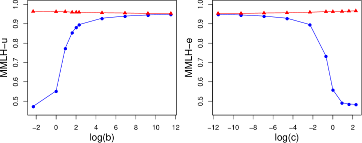
Figure 2: Cascade structure for $p=7$ and $T=200$. F1 score (blue lines) and TP-score (red lines) as functions of the uniform prior parameter $b$ (left panel) and exponential prior parameter $c$ (right panel). The x-axes are reported in log-scale.

Mid-dense setting

Now, we investigate a default scenario considered in Jalaldoust et al. (2022). In this setting, all diagonal entries of the influence matrix $\boldsymbol{\alpha}$ are non-zero, i.e. all nodes are self-excitatory. All non-diagonal entries of the adjacency matrix of the underlying connectivity graph are randomly drawn from a Bernoulli distribution with success probability 0.3. In the case of a success (one), the corresponding $\alpha_{ij}$ is drawn from $U([0.1,0.2])$ (and so are the $\alpha_{ii}$). Moreover, each entry $\mu_{i}$ of the baseline vector $\boldsymbol{\mu}$ is drawn from $U([0.5,1.0])$ and all $\beta_{ij}$ are again set to $1$. Here, we further set the prior parameters $b$ and $c$ to $4$ and $0.3$, respectively, reducing thus the penalty strength on structures $\boldsymbol{\gamma}_{i}$ with a larger number of non-zero entries. This is motivated by the fact that this scenario may be considered as a mid-dense setting, since the ground truth connectivity matrices contain on average $p+0.3p(p-1)$ connections. In the case of $p=7$, this corresponds to an average of $40\%$ of edges.

The results are reported in Table 3 for different values of $T$. We observe that the method with the highest F1-accuracy is MDLH. Moreover, on shorter time horizons $T$, MMLH is also outperformed by ADM4 and MLE-thr. However, for $T\geq 1000$, the only rival is MDLH, which gives a score close to $0.95$ (MMLH, in comparison, is approaching $0.9$). For the chosen prior parameters, we observe a slightly better performance for MMLH-u than for MMLH-e, except for the case $T=200$.

In Figure 3, we report again the impact of $b$ (left panel) and $c$ (right panel) on the F1 score (blue lines) and TP score (red lines) for the case $T=200$. The previously considered values $b=4$ and $c=0.3$ are marked as vertical grey dashed lines. Remarkably, while in the sparse scenarios BIC almost reached the performance of MMLH, both MMLH-u and MMLH-e outperform BIC in this mid-dense setting for all considered values of $b$ and $c$ (though only slightly for large $b$ and small $c$).

	F1 score
$p=$	7
$T=$	$200$	$400$	$700$	$1000$	$1200$	$1400$
MMLH-u	0.567	0.692	0.775	0.833	0.857	0.872
MMLH-e	0.579	0.692	0.766	0.812	0.841	0.847
MLE-ms	0.597	0.670	0.735	0.767	0.795	0.804
MLE-thr	0.629	0.729	0.792	0.824	0.836	0.864
BIC	0.399	0.471	0.535	0.613	0.645	0.707
ADM4	0.699	0.758	0.770	0.783	0.785	0.786
MDLH	0.764	0.846	0.893	0.927	0.945	0.951

Table 3: Mid-dense setting 3: Bernoulli random structure. The values for the uniform and exponential priors are $b=4$ and $c=0.3$, respectively.

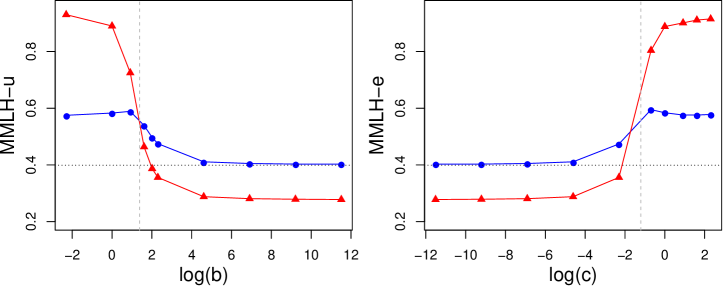
Figure 3: Bernoulli random structure for $p=7$ and $T=200$. F1 score (blue lines) and TP score (red lines) as functions of the uniform prior parameter $b$ (left panel) and exponential prior parameter $c$ (right panel). The vertical grey dashed lines indicate the investigated values $b=4$ and $c=0.3$, and the horizontal black dotted lines correspond to the F1 score for BIC. The x-axes are reported in log-scale.

6.2 Experiments with Real-World Data

The goal of this subsection is to illustrate how the proposed MMLH approach performs on real-world data. In particular, we consider 10-year (2003-2014) sovereign bond yield volatilities of seven large economies called the Group of Seven (G7), being composed of the US, Canada, Germany, France, Japan, UK and Italy. This dataset has been investigated in Demirer et al. (2018) and also analysed in Jalaldoust et al. (2022). It is publicly available at: http://qed.econ.queensu.ca/jae/2018-v33.1/demirer-et-al/

Figure 4: Connectivity graph derived from Umar et al. (2022) (an edge is drawn if it appears in at least one of the three graphs shown in their Figure 1).

As this dataset corresponds to time series data, we pre-process it to identify shocks (i.e. events able to be reproduced by a point process) in the return volatilities. In particular, following Jalaldoust et al. (2022), for each country we roll a one-year window over the respective data and register an event if the latest value of the window is among the top 20% of values in the rolling window. The resulting number of events registered for each country is roughly $500$. Following Jalaldoust et al. (2022), we assume that this data is observed within a time horizon of $T=400$ of the investigated exp-MHP, i.e. an instance of a short time horizon.

Our study is conducted as follows: We compare MMLH with the methods MDLH, BIC, and ADM4 as well as with available expert knowledge. For MMLH, BIC and ADM4, we prepare the data as described above and launch the respective causal discovery algorithm. For MDLH, we rely on the results reported in Jalaldoust et al. (2022). Moreover, as “expert knowledge” we consider the conclusions reported in Umar et al. (2022), where the network connectedness between sovereign bond yield curve components of the G7 countries is discussed. The connectivity graph derived from Umar et al. (2022) is shown in Figure 4. The results of the investigated methods are presented in Figure 5, with the graphs in the top panels corresponding to ADM4 (left), MDLH (middle), and BIC (right). In the bottom panels, we report the results for MMLH-e with $c=10^{-5}$ (left), $c=0.3$ (middle), and $c=2.5$ (right). As expected, similar results are obtained for MMLH-u. For example, using $b=10^{5}$ we obtain the same graph as reported in the bottom left panel, and for $b=4$ the same as shown in the bottom middle panel, except for the connection “ITA to FRA” not being present. Note that the red connections in the graphs visualized in Figure 5 are those that are in agreement with the expert knowledge graph of Figure 4.

Figure 5: Connectivity graph for ADM4 (top left panel), MDLH (top middle panel), BIC (top right panel), MMLH-e with $c=10^{-5}$ (bottom left panel), $c=0.3$ (bottom middle panel), and $c=2.5$ (bottom right panel). The red connections are those that are in agreement with Umar et al. (2022).

We observe that ADM4 yields the most connections in agreement with Umar et al. (2022), however it also suggests $6$ connections that are not present in Figure 4. As expected from the synthetic experiments, for small $c$ (resp. large $b$) (i.e., when we have a strong penalty on structures $\boldsymbol{\gamma}_{i}\in\boldsymbol{\Gamma}_{i}=\{0,1\}^{p}$ with many non-zero entries), MMLH performs similar to BIC, which only suggests one connection not present in Figure 4 (“US to GER”). Increasing $c$ to $0.3$ (resp. decreasing $b$ to $4$) adds further connections to the graph (bottom middle panel), of which all are reported in Umar et al. (2022). In particular, for $c=0.3$ MMLH-e yields $9$ connections present in Figure 4 (and a single one that is not reported there). In comparison, MDLH only captures $7$ connections of Figure 4 (and also reports one wrong connection). Thus, the proposed MMLH algorithm not only outperforms the classical BIC method, but also reports more connections that are in agreement with the literature than the related state-of-the-art MDLH method. Note also that $6$ out of $8$ connections detected by MDLH are in agreement with MMLH-e for $c=0.3$, see the middle panels of Figure 5.

Moreover, we observe that many outgoing connections from France are captured well by ADM4, MDLH and MMLH. Further, the outgoing connections from Germany are only (partially) captured by ADM4. However, this improves for MMLH when further increasing $c$ (resp. decreasing $b$). In particular, using $c=2.5$ and $b=0.25$, we obtain the connections “GER to ITA” and “GER to JPA”. We also observe that Japan is isolated from the other countries, except under ADM4 and MMLH, which report an ingoing connection from the US, in agreement with Umar et al. (2022). Only MMLH-e (for $c=2.5$) reports a second ingoing connection (from Germany), which is also present in Figure 4. These observations also suggest a solid performance of the proposed MMLH procedure.

7 Conclusion and Discussion

In this paper, we estimated Granger causal relations between components of multivariate Hawkes processes with exponential decay kernels. These relations are described by a connectivity graph, which can be estimated from observations of the process. We approached this problem by proposing an optimization criterion and a model selection algorithm MMLH based on the minimum message length principle.

In contrast to other model selection algorithms, MMLH incorporates prior distributions of the underlying model parameters, making the procedure Bayesian. While classical model selection criteria (e.g. BIC) are designed to penalize models with a lot of parameters (i.e. structures with many non-zero entries) and thus do not take into account other descriptions of the model, MMLH offers more flexibility in terms of structure-related penalty. This may be particularly beneficial, if some a-priori expert knowledge on the structure of the underlying graph exists. Given the fact that all model parameters to be estimated are non-negative, we investigated both a uniform prior and an exponential prior and observed a similar performance for both of them in all our experiments.

We conducted synthetic experiments in which we compared the proposed algorithm to other related classical and state-of-art methods, focusing on short time horizons. In the considered sparse graph scenarios, MMLH achieved the highest F1 scores among all comparison methods. Concerning the investigated mid-dense scenario, MMLH showed an F1 precision comparable to MLE-ms, MLE-thr and ADM4. However, MMLH outperformed them with increasing number of events, the only rival being the state-of-art MDLH. The superior F1 precision of MMLH on sparse connectivity graphs may be explained by the fact that the minimum message length principle prefers short encodings of the model (i.e. sparse graphs) over longer encodings (i.e. non-sparse graphs) together with a short description of the data using the model.

Finally, we illustrated the proposed method on G7 sovereign bond data and compared the inferred causal connections to those of MDLH, ADM4 and BIC. We demonstrated that the connectivity graphs obtained via MMLH (with three different parameterizations of the prior function) are in agreement with the expert knowledge extracted from the literature.

As a possible future work one may investigate connectivity graphs in multivariate Hawkes processes with other kernels or intensities given by non-linear functional relationships (e.g., ReLU or sigmoid functions). Another research direction is a modification of the algorithm which allows to increase the performance on non-sparse structures.

Acknowledgments

K. H.-S. acknowledges a partial support by the Austrian Science Foundation FWF (project I5113), by the Czech Science Foundation, (project GA19-16066S) and by the Czech Academy of Sciences, Praemium Academiae awarded to M. Paluš. A part of this paper was written while I.T. was member of the Institute of Stochastics, Johannes Kepler University Linz, 4040 Linz, Austria. During this time, I.T. was supported by the Austrian Science Fund (FWF): W1214-N15, project DK14.

References

- Achab et al. (2017) Massil Achab, Emmanuel Bacry, Stephane Gaiffas, Iacopo Mastromatteo, and Jean-Francois Muzy. Uncovering causality from multivariate Hawkes integrated cumulants. In International Conference on Machine Learning, pages 1–10. PMLR, 2017.
- Aho and Hopcroft (1974) Alfred V. Aho and John E. Hopcroft. The Design and Analysis of Computer Algorithms. Pearson Education India, 1974.
- Bacry et al. (2020) Emmanuel Bacry, Martin Bompaire, Stephane Gaïffas, and Jean-Francois Muzy. Sparse and low-rank multivariate Hawkes processes. Journal of Machine Learning Research, 21(50):1–32, 2020.
- Conway and Sloane (1984) John Horton Conway and Neil James Alexander Sloane. On the Voronoi regions of certain lattices. SIAM Journal on Algebraic Discrete Methods, 5(3):294–305, 1984.
- Demirer et al. (2018) Mert Demirer, Francis X. Diebold, Laura Liu, and Kamil Yilmaz. Estimating global bank network connectedness. Journal of Applied Econometrics, 33(1):1–15, 2018.
- Didelez (2008) Vanessa Didelez. Graphical models for marked point processes based on local independence. Journal of the Royal Statistical Society: Series B (Statistical Methodology), 70(1):245–264, 2008.
- Eichler et al. (2017) Michael Eichler, Rainer Dahlhaus, and Johannes Dueck. Graphical modeling for multivariate Hawkes processes with nonparametric link functions. Journal of Time Series Analysis, 38(2):225–242, 2017.
- Grünwald (2007) Peter Grünwald. The Minimum Description Length Principle. MIT Press, 2007.
- Grünwald and Roos (2019) Peter Grünwald and Teemu Roos. Minimum description length revisited. International Journal of Mathematics for Industry, 11(01):1930001, 2019.
- Hansen et al. (2015) Niels Richard Hansen, Patricia Reynaud-Bouret, and Vincent Rivoirard. Lasso and probabilistic inequalities for multivariate point processes. Bernoulli, 21(1):83–143, 2015.
- Hawkes (1971) Alan G. Hawkes. Spectra of some self-exciting and mutually exciting point processes. Biometrika, 58(1):83–90, 1971.
- Hlaváčková-Schindler and Plant (2020a) Kateřina Hlaváčková-Schindler and Claudia Plant. Heterogeneous graphical Granger causality by minimum message length. Entropy, 22(12):1400, 2020a.
- Hlaváčková-Schindler and Plant (2020b) Kateřina Hlaváčková-Schindler and Claudia Plant. Graphical Granger causality by information-theoretic criteria. In ECAI 2020, pages 1459–1466. IOS Press, 2020b.
- Idé et al. (2021) Tsuyoshi Idé, Georgios Kollias, Dzung T. Phan, and Naoki Abe. Cardinality-regularized Hawkes-Granger model. Advances in Neural Information Processing Systems, 34:2682–2694, 2021.
- Jalaldoust et al. (2022) Amirkasra Jalaldoust, Kateřina Hlaváčková-Schindler, and Claudia Plant. Causal discovery in Hawkes processes by minimum description length. In Proceedings of the 36th AAAI Conference on Artificial Intelligence, pages 6978–6987. PKP Publishing Services Network, 2022.
- Juditsky et al. (2020) Anatoli Juditsky, Arkadi Nemirovski, Liyan Xie, and Yao Xie. Convex parameter recovery for interacting marked processes. IEEE Journal on Selected Areas in Information Theory, 1(3):799–813, 2020.
- Li and Vitányi (2008) Ming Li and Paul Vitányi. An Introduction to Kolmogorov Complexity and Its Applications, volume 3. Springer, 2008.
- Makalic and Schmidt (2021) Enes Makalic and Daniel Francis Schmidt. Minimum message length inference of the exponential distribution with type I censoring. Entropy, 23(11):1439, 2021.
- Ogata (1981) Yosihiko Ogata. On Lewis’ simulation method for point processes. IEEE Transactions on Information Theory, 27(1):23–31, 1981.
- Ogata (1988) Yosihiko Ogata. Statistical models for earthquake occurrences and residual analysis for point processes. Journal of the American Statistical association, 83(401):9–27, 1988.
- Oliver et al. (1996) Jonathan J. Oliver, Rohan A. Baxter, and Chris S. Wallace. Unsupervised learning using MML. In International Conference on Machine Learning, pages 364–372, 1996.
- Ozaki (1979) Taisuke Ozaki. Maximum likelihood estimation of Hawkes’ self-exciting point processes. Annals of the Institute of Statistical Mathematics, 31(1):145–155, 1979.
- Reid et al. (2016) Stephen Reid, Robert Tibshirani, and Jerome Friedman. A study of error variance estimation in lasso regression. Statistica Sinica, pages 35–67, 2016.
- Rissanen (1998) Jorma Rissanen. Stochastic Complexity in Statistical Inquiry, volume 15. World Scientific, 1998.
- Roos et al. (2009) Teemu Roos, Petri Myllymaki, and Jorma Rissanen. MDL denoising revisited. IEEE Transactions on Signal Processing, 57(9):3347–3360, 2009.
- Shlomovich et al. (2022) Leigh Shlomovich, Edward A. K. Cohen, and Niall Adams. A parameter estimation method for multivariate binned Hawkes processes. Statistics and Computing, 32:98, 2022. doi: 10.1007/s11222-022-10121-2.
- Singer and Singer (1999) Sanja Singer and Saša Singer. Complexity analysis of Nelder-Mead search iterations. In Proceedings of the first Conference on Applied Mathematics and Computation, pages 185–196. PMF–Matematicki Odjel Zagreb, Croatia, 1999.
- Sulem et al. (2021) Deborah Sulem, Vincent Rivoirard, and Judith Rousseau. Bayesian estimation of nonlinear Hawkes process. arXiv preprint arXiv:2103.17164, 2021.
- Trouleau et al. (2021) William Trouleau, Jalal Etesami, Matthias Grossglauser, Negar Kiyavash, and Patrick Thiran. Cumulants of Hawkes processes are robust to observation noise. In International Conference on Machine Learning, pages 10444–10454. PMLR, 2021.
- Umar et al. (2022) Zaghum Umar, Yasir Riaz, and David Y Aharon. Network connectedness dynamics of the yield curve of G7 countries. International Review of Economics & Finance, 79:275–288, 2022.
- Veen and Schoenberg (2008) Alejandro Veen and Frederic P. Schoenberg. Estimation of space–time branching process models in seismology using an EM–type algorithm. Journal of the American Statistical Association, 103(482):614–624, 2008.
- Wallace (2005) Chris S. Wallace. Statistical and Inductive Inference by Minimum Message Length. Springer, 2005.
- Wallace and Boulton (1968) Chris S. Wallace and D.M. Boulton. An information measure for classification. The Computer Journal, 11(2):185–194, 1968.
- Wallace and Dowe (1999) Chris S. Wallace and David L. Dowe. Minimum message length and Kolmogorov complexity. The Computer Journal, 42(4):270–283, 1999.
- Wallace and Freeman (1987) Chris S. Wallace and P.R. Freeman. Estimation and inference by compact coding. Journal of the Royal Statistical Society: Series B (Methodological), 49(3):240–252, 1987.
- Wang et al. (2020) Haoyun Wang, Liyan Xie, Alex Cuozzo, Simon Mak, and Yao Xie. Uncertainty quantification for inferring Hawkes networks. Advances in Neural Information Processing Systems, 33:7125–7134, 2020.
- Wei et al. (2023) Song Wei, Yao Xie, Christopher S. Josef, and Rishikesan Kamaleswaran. Granger causal chain discovery for sepsis-associated derangements via continuous-time Hawkes processes. In Proceedings of the 29th ACM SIGKDD Conference on Knowledge Discovery and Data Mining, pages 2536–2546, 2023.
- Xu et al. (2016) Hongteng Xu, Mehrdad Farajtabar, and Hongyuan Zha. Learning Granger causality for Hawkes processes. In International Conference on Machine Learning, pages 1717–1726. PMLR, 2016.
- Zhou et al. (2013) Ke Zhou, Hongyuan Zha, and Le Song. Learning social infectivity in sparse low-rank networks using multi-dimensional Hawkes processes. In Artificial Intelligence and Statistics, pages 641–649. PMLR, 2013.