Reconstruction of Unstable Heavy Particles Using Deep Symmetry-Preserving Attention Networks

Abstract

Reconstructing unstable heavy particles requires sophisticated techniques to sift through the large number of possible permutations for assignment of detector objects to the underlying partons. An approach based on a generalized attention mechanism, symmetry preserving attention networks (Spa-Net), has been previously applied to top quark pair decays at the Large Hadron Collider which produce only hadronic jets. Here we extend the Spa-Net architecture to consider multiple input object types, such as leptons, as well as global event features, such as the missing transverse momentum. In addition, we provide regression and classification outputs to supplement the parton assignment. We explore the performance of the extended capability of Spa-Net in the context of semi-leptonic decays of top quark pairs as well as top quark pairs produced in association with a Higgs boson. We find significant improvements in the power of three representative studies: a search for $t\bar{t}H$, a measurement of the top quark mass, and a search for a heavy $Z^{\prime}$ decaying to top quark pairs. We present ablation studies to provide insight on what the network has learned in each case.

1 Introduction

Event reconstruction is a crucial problem at the Large Hadron Collider (LHC), where heavy, unstable particles such as top quarks, Higgs bosons and electroweak $W$ and $Z$ bosons decay before being directly measured by the detectors. Measuring properties of these particles requires reconstructing their four-momenta from their immediate decay products, which we refer to as partons. Since many partons leave indistinguishable signatures in detectors, a central difficulty is assigning the observed detector objects to each parton. As the number of partons grows, the combinatorics of the problem becomes overwhelming and the inability to efficiently select the correct assignment dilutes valuable information.

Previously, methods such as $\chi^{2}$ fits Snyder:1995hg or kinematic likelihoods klfitter have provided analytic approaches for performing this task. These approaches are limited, however, by the requirement of exhaustively building each possible permutation of the event, and by the limited amount of kinematic information that can be incorporated. Particularly at high energy hadron colliders such as the LHC, events often contain many extra objects from additional activity as well as the particles originating from the hard scattering event, which can cause the performance of permutation-based methods to degrade substantially.

This work presents a complete machine learning approach to event reconstruction at the LHC, named Spa-Net due to its use of a symmetry preserving attention mechanism, designed to incorporate all of the symmetries present in the problem. It was first introduced spanet1 ; spanet2 in the context of reconstruction of the all-hadronic final state in which only one type of object is present. In this work, we extend and complete the method by generalizing to arbitrary numbers of object types, as well as adding multiple capabilities that can aid the application of Spa-Net in LHC data analysis, including signal and background discrimination, kinematic regression, and auxiliary outputs to separate different kinds of events.

To demonstrate the new capacity of the technique, we study its performance in final states containing a lepton and a neutrino. The method is compared to existing baseline approaches and demonstrated to provide significant improvements in three flagship LHC physics measurements: $t\bar{t}H$ cross-section, top quark mass, and a search for a hypothetical $Z^{\prime}$ boson decaying to top quark pairs. These examples demonstrate various additional features, such as kinematic regression and signal versus background discrimination. The method can be applied to any final state at the LHC or other particle collider experiments, and may be applicable to other set assignment tasks in other scientific fields.

This paper is organised as follows. The extensions of the Spa-Net architecture introduced since Ref. spanet2 are described in Section 2, while the baseline methods used for comparison are introduced in Section 3. The datasets used in the studies presented are described in Section 4. Section 5 presents the basic performance metrics and compares Spa-Net to the baselines, while Section 6 presents several studies performed to understand Spa-Net learning strategies. The Sections 7, 8 and 9 respectively demonstrate the expected impact of Spa-Net to the $t\bar{t}H$, top mass, and $Z^{\prime}$ analyses. Finally we give some concluding remarks in Section 10.

2 Spa-Net Extensions

We present several improvement to the base Spa-Net architecture to tackle the additional challenges inherent to events containing multiple reconstructed object classes and to allow for a greater variety of outputs for an array of potential auxiliary tasks. These modifications allow Spa-Net to be applied to essentially any topology and allow for analysis of many additional aspects of events beyond the original jet-parton assignment task.

2.1 Input Observables

While the original Spa-Net spanet1 ; spanet2 studies concentrated on examples where all objects have hadronic origins, we focus here on the challenges of semi-leptonic topologies. These events contain several different reconstructed objects, including the typical hadronic jets as well as leptons and missing transverse momentum ($E_{\mathrm{T}}^{\mathrm{miss}}$) typically associated with neutrinos. Unlike jets or leptons, this $E_{\mathrm{T}}^{\mathrm{miss}}$ is a global observable, and its multiplicity does not vary event by event.

We accommodate these additional inputs by training individual position-independent embeddings for each class of input. This allows the network to adjust to the various distributions for each input type, and allows us to define sets of features specific to each type of object. We parameterise jets using the same $\{M,p_{\mathrm{T}},\eta,\sin\phi,\cos\phi,b\textrm{-tag}\}$ representation as in Ref. spanet2 , where $M$ is the jet mass, $p_{\mathrm{T}}$ is the jet momentum transverse to the incoming proton beams, and $\phi$ is the azimuthal angle around the detector, represented by its trigonometric components to avoid the boundary condition at $\phi=\pm\pi$. $\eta$ is the pseudo-rapidity pseudorap of the jet, the standard measure of the polar angle between the incoming proton beam and the jet commonly used in particle physics due to its Lorentz-invariant quantities. Leptons are similarly represented using $\{M,p_{\mathrm{T}},\eta,\sin\phi,\cos\phi,\textrm{flavor}\}$ where flavor is $0$ for electrons and $1$ for muons. Finally, $E_{\mathrm{T}}^{\mathrm{miss}}$ is represented using two scalar values, the magnitude and azimuthal angle, and is treated as an always-present jet or lepton. The individual embedding layers map these disparate objects with different features into a unified latent space which may be processed by the central transformer.

The global inputs, such as $E_{\mathrm{T}}^{\mathrm{miss}}$, need to be treated differently than the jets and leptons, as they do not have associated parton assignments. Therefore, after computing the central transformer, we do not include the extra global $E_{\mathrm{T}}^{\mathrm{miss}}$ vector in the particle transformers. This allows the transformer to freely share the $E_{\mathrm{T}}^{\mathrm{miss}}$ information with the other objects during the central transformer step while preventing it from being chosen as a reconstruction object for jet-parton assignment.

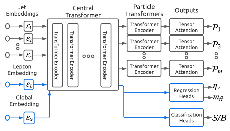
Figure 1: Extended diagram of the new Spa-Net architecture showing the additional embeddings as well as outputs for classification and regression.

2.2 Secondary Outputs

Beyond jet-parton assignment, we are interested in reconstruction of further observables, such as the unknown neutrino $\eta$, or differentiation of signal events from background.

To accomplish this, we add additional output heads to the central transformer which are trained end-to-end simultaneously with the base reconstruction task. We extract an event embedding from the central transformer by including a learnable event vector in the inputs to the transformer. We append this learned event vector $\mathcal{E}_{E}\in\mathbb{R}^{D}$ to the list of embedded input vectors: $\mathcal{E}=\{\mathcal{E}_{1},\mathcal{E}_{2},\dots,\mathcal{E}_{n},\mathcal{E}_{L},\mathcal{E}_{G},\mathcal{E}_{E}\}$ prior to the central transformer (Figure 1). This allows the central transformer to process this event vector using all of the information available in the observables.

We extract the encoded event vector after the central transformer and treat it as a latent summary representation of the entire event $z_{E}$. We can then feed these latent features into simple feed-forward neural networks to perform signal vs background classification, kinematic regression, or any other downstream task.

These additional feed forward networks are trained using their respective loss, either categorical log-likelihood or mean squared error (MSE). These auxiliary losses are simply added to the total Spa-Net loss, weighted by their respective hyperparameter $\alpha_{i}$. With the parton reconstruction loss, $\mathcal{L}_{\textrm{reconstruction}}$ defined as the masked minimum permutation loss from Equation 6 of Ref. spanet2 , the Spa-Net loss becomes:

$$\mathcal{L}=\alpha_{0}\mathcal{L}_{\textrm{reconstruction}}+\alpha_{1}\mathcal{L}_{\textrm{classification}}+\alpha_{2}\mathcal{L}_{\textrm{regression}}.$$ (1)

2.3 Particle Detector

In Ref. spanet2 , we introduced the ability to reconstruct partial events by splitting the reconstruction task based on the event topology. This is a powerful technique that is particularly useful in complex events, where it is very likely that at least one of the partons will not have a corresponding detector object.

However, the assignment outputs are trained only on examples in which the event contains all detector objects necessary for a correct parton assignment. We refer to the reconstruction target particles in these examples as reconstructable. We must train this way because only reconstructable particles have truth-labelled detector objects, which are required for training, and we ignore non-reconstructable particles via the masked loss defined in Equation 6 of Ref. spanet2 . As a result of this training procedure, the Spa-Net assignment probability $P_{a}$ only represents a conditional assignment distribution over jet indices $j_{i}$ for each particle $p$ given that the particle is reconstructable:

$$P_{a}(j_{1},j_{2},\dots,j_{k_{p}}\mid p\text{ reconstructable}).$$ (2)

We use $P(p\text{~{}reconstructable})=P(p)$ and $P(p\text{ not reconstructable})=P(\neg p)$ for conciseness. To construct an unconditional assignment distribution, we need to additionally estimate the probability that a given particle is reconstructable in the event, $P_{d}$. This additional distribution may be used to produce a pseudo-marginal probability for the assignment. While $P_{a}(j_{1},j_{2},\dots,j_{k_{p}}\mid\neg p)=0$ is not a valid distribution, and therefore this marginal probability is ill-defined, we may still use this pseudo-marginal probability

$$\mathcal{P}(j_{1},j_{2},\dots,j_{k_{p}})=P_{a}(j_{1},j_{2},\dots,j_{k_{p}}\mid p)P_{d}(p)$$ (3)

as an overall measurement of the assignment confidence of the network.

We aim to estimate this reconstruction probability, $P_{d}(p)$, with an additional output head of Spa-Net. We will refer to this output as the detection output, because it is trained to detect whether or not a particle is reconstructable in the event. We train this detection output in a similar manner as the classification outputs but at the particle level instead of the event level. That is, we extract a summary particle vector from each of the particle transformer encoders using the same method as the event summary vector from the central transformer. We then feed these particle vectors into a feed-forward binary classification network to produce a Bernoulli probability for each particle. We have to also take into account the potential event-level symmetries in a similar manner to the assignment reconstruction loss from Equation 6 of Ref. spanet2 . We train this detection output with a cross-entropy loss over the symmetric particle masks:

$$\mathcal{L}_{\textrm{detection}}=\min_{\sigma\in G_{E}}{\left[\mathcal{M}_{\sigma(p)}\log P_{d}(p)+(1-\mathcal{M}_{\sigma(p)})\log\left(1-P_{d}(p)\right)\right]}.$$ (4)

The complete loss equation for the entire network can now be defined:

$$\mathcal{L}=\alpha_{0}\mathcal{L}_{\textrm{reconstruction}}+\alpha_{1}\mathcal{L}_{\textrm{detection}}+\alpha_{2}\mathcal{L}_{\textrm{classification}}+\alpha_{3}\mathcal{L}_{\textrm{regression}}.$$ (5)

3 Baseline Methods

We compare Spa-Net to two commonly-used methods, the Kinematic Likelihood Fitter (KLFitter) klfitter , and a “Permutation Deep Neural Network” (PDNN), which uses a fully-connected deep neural network similar to Ref. permdnn . Both methods are permutation based, meaning they sequentially evaluate every possible permutation of particle assignments. The performance of these algorithms is compared to Spa-Net in terms of reconstruction efficiency (Section 5), the separation of various event categories (Section 5.2) and the run times (Section 5.3), as well as the final sensitivity of the three considered analyses (Sections 7, 8, 9).

3.1 KLFitter

KLFitter has been extensively used in top quark analyses ATLAS_ana1_klf ; ATLAS:2014rkz ; ATLAS:2014aus ; ATLAS_ana2_klf ; ATLAS:2019hxz ; ATLAS_ana3_klf ; CMS_ana_klf ; CMS:2020ezf ; ATLAS:2017gkv , especially for semi-leptonic $t\bar{t}$ events. The method involves building every possible permutation of the event and constructing a likelihood score for each. The permutation with the maximum likelihood is thus taken as the best reconstruction for that event. The likelihood score is defined as:

$$\begin{split}\mathcal{L}&=B(m_{q_{1}q_{2}q_{3}}\textrm{\textbar}m_{t},\Gamma_{t})\cdot B(m_{q_{1}q_{2}}\textrm{\textbar}m_{W},\Gamma_{W})\\ &\times B(m_{q_{4}\ell\nu}\textrm{\textbar}m_{t},\Gamma_{t})\cdot B(m_{\ell\nu}\textrm{\textbar}m_{W},\Gamma_{W})\\ &\times\prod_{i=1}^{4}W_{jet}(E_{jet,i}^{meas}\textrm{\textbar}E_{jet,i})\cdot W_{\ell}(E_{\ell}^{meas}\textrm{\textbar}E_{\ell})\\ &\times W_{miss}(E_{x}^{miss}\textrm{\textbar}p_{x}^{\nu})\cdot W_{miss}(E_{y}^{miss}\textrm{\textbar}p_{y}^{\nu}),\end{split}$$ (6)

where $B$ represent Breit-Wigner functions, $m_{q_{1}q_{2}q_{3}}$, $m_{q_{1},q_{2}}$, $m_{q_{4}\ell\nu}$, $m_{\ell\nu}$ are invariant masses computed from the final state particle momenta. The variables $m_{t(W)}$ and $\Gamma_{t(W)}$ are the masses and decay widths of the top quark ($W$ boson) respectively. The expressions $E_{\ell,jet}$ represents the energy of the leptons or jets respectively, and the functions $W_{var}(var_{A}\textrm{\textbar}var_{B})$ are the transfer function for the variable $var_{A}$ from $var_{B}$.

This method suffers from several limitations. Firstly, the requirement to construct and test every possible permutation leads to a run-time that grows exponentially with the number of jets or other objects in the event. This quickly becomes a limiting factor in large datasets, which at the LHC often contain millions of events that must be evaluated hundreds of times each (once per systematic uncertainty shift). While semi-leptonic $t\bar{t}$ can largely remain tractable, it can significantly slow down analyses due to the heavy computing cost, and it is typical to limit the evaluation to only a subset of the reconstructed objects in order to reduce this burden, which restricts the number of events that can be correctly reconstructed. More complex final states, for example $t\bar{t}H$ production, require even more objects to be reconstructed and thus take even longer to compute, severely limiting the usability of the method in such channels.

A second limitation of the method is its treatment of partial events, which the likelihood is not designed to handle, and thus performance in these events is significantly degraded. Finally, the method does not take into account any correlations between the decay products of the target particles and the rest of the event, since only the particles hypothesised as originating from the targets are included in the likelihood evaluation. An advantage of the method is the use of transfer functions to represent detector effects, but these must be carefully derived for each detector to achieve maximum performance, which can be a difficult and time-consuming endeavour.

There are two variations of the KLFitter likelihood of interest in our studies: one in which the top quark mass is given an assumed value, and one in which it is not. Specifying the assumed mass leads to improved reconstruction efficiency at the expense of biasing towards permutations at this mass, causing sculpting of backgrounds and other undesirable effects. In the analyses presented in Sections 7 and 9, the top quark mass is fixed to a value of 173 GeV, since this biasing is less important than overall reconstruction efficiency. In contrast, the top quark mass measurement presented in Section 8 must avoid biasing towards a specific mass value, and thus the mass is not fixed in the likelihood for this analysis.

3.2 Permutation DNN

The Permutation DNN (PDNN) uses a fully connected deep neural network which takes the kinematic and tagging information of the reconstructed objects as inputs, similar to the method described in Ref. permdnn . Again, each possible permutation of the event is evaluated, and the assignment with the highest network output score is taken as the best reconstruction. Training is performed as a discrimination task, in which the correct permutations are marked as signal and all of the other permutations are marked as background.

This method also suffers from several limitations, including the same exponentially growing run-time due to the permutation-based approach, the inability to adequately handle partial events, and the lack of inputs related to additional event activity. Further, the method does not incorporate the symmetries of the reconstruction problem, due to the way in which input variables must be associated to the hypothesised targets. Recently, message passing graph neural networks were applied to the all-hadronic $t\bar{t}$ final state topographs , but as all studies presented here are performed in the lepton+jets channel, no comparison is made to such methods.

4 Datasets

Several datasets of simulated collisions are generated to test a variety of experimental analyses and effects. All datasets are generated at a centre-of-mass energy of $\sqrt{s}=13$ TeV using MadGraph_aMC@NLO Alwall:2014hca (v3.2.0, NCSA license) for the matrix element calculation, Pythia8 Sjostrand:2014zea (v8.2, GPL-2) for the parton showering and hadronisation, and Delphes deFavereau:2013fsa (v3.4.2, GPL-3) using the default CMS detector card for the simulation of detector effects. For all samples, jets are reconstructed using the anti-$k_{\textrm{T}}$ jet algorithm Cacciari:2008gp with a radius parameter of $R=0.5$, a minimum transverse momentum of $p_{\mathrm{T}}$$>$25 GeV, and an absolute pseudo-rapidity of $|\eta|$$<$2.5. To identify jets originating from $b$-quarks, a “$b$-tagging” algorithm with a $p_{\mathrm{T}}$ and ($\eta,\phi$) dependent efficiency and mis-tagging rate is applied. Electrons and muons are selected with the same $p_{\mathrm{T}}$ and $\eta$ requirements as for jets. No requirement is placed upon the missing transverse momentum $E_{\mathrm{T}}^{\mathrm{miss}}$.

A large sample of simulated Standard Model (SM) $t\bar{t}$ production is generated with the top quark mass $m_{t}=173$ GeV, and used for reconstruction studies presented in Section 5 as well as the background model in the $Z^{\prime}$ studies presented in Section 9. It contains approximately 11M events after a basic event selection of exactly one electron or muon and at least four jets of which at least two are $b$-tagged. We further produce samples of approximately 0.2M events at mass points of $m_{t}=170,171,172,173,174,175,176$ GeV in order to build templates for the top mass analysis presented in Section 8. Finally, we generate a sample of approximately 12M $t\bar{t}$ events with an approximately flat $m_{t}$ distribution in the 166-176 GeV range by producing events in steps of 0.1 GeV. A final sample with $m_{t}$$=171.9$ GeV was produced to be used as pseudo-data for the top mass analysis. The value used was initially known by only one member of the team to avoid bias in the final mass extraction.

A sample of simulated SM $t\bar{t}H$ production, in which the Higgs boson decays to a pair of $b$-quarks, is generated to model the signal process for the $t\bar{t}H$ analysis presented in Section 7. This sample has the same event selection as applied to the $t\bar{t}$ samples, with an additional requirement of at least six jets due to the additional presence of the Higgs boson. Training of Spa-Net is performed using 10M $t\bar{t}H$ events with at least two $b$-tagged jet, while the final measurement described in Section 7 is performed using a distinct sample where 0.2M of 1.1M events satisfy the more stringent requirement of containing least four $b$-tagged jets. Training with the two-tag requirement achieved better overall performance than on the tighter four-tag selection which follows the most recent ATLAS analyses in this channel ATLAS:2021qou . The background in this analysis is dominated by $t\bar{t}+b\bar{b}$ production, which is modeled using a simulated sample in which the top and bottom pairs are explicitly included in the hard process generated by MadGraph_aMC@NLO; of the 1.3M events generated, 0.2M survive the event selection.

Finally, we produce Beyond the Standard Model (BSM) events containing a hypothetical $Z^{\prime}$ boson that decays to a pair of top quarks, using the vPrimeNLO model vprimeNLO in MadGraph_aMC@NLO. One sample of 0.2M events is produced at each of $m_{Z^{\prime}}=500,700,900$ GeV to evaluate search sensitivity at a range of masses. A sample with an approximately flat $m_{Z^{\prime}}$ distribution is generated for network training by generating events in 1 GeV steps between 400 and 1000 GeV.

We match jets to the original decay products of the top quarks and Higgs bosons using an exclusive $\Delta R=(\sqrt{(\phi_{j}-\phi_{d})^{2}+(\eta_{j}-\eta_{d})^{2}}<0.4$ requirement, such that only one decay product can be matched to each jet and vice versa, always taking the closest match. This allows a crisp definition of the correct assignments as well as categorisation of events based upon which particles are reconstructable, as explained in Section 2.3.

5 Reconstruction and Regression Performance

We present the reconstruction efficiency for Spa-Net in semi-leptonic $t\bar{t}$ and $t\bar{t}H(H\rightarrow b\bar{b})$ events, compared to the performance of benchmark methods KLFitter and PDNN described in Section 3. Efficiencies are presented relative to all events in the generated sample, as well relative to the subset of events in which all top quark (and Higgs boson in the case of $t\bar{t}H$) daughters are truth-matched to reconstructed jets, which we call “Full Events”. We also show efficiencies for each type of particle, with $t_{\mathrm{H}}$ the hadronically decaying top quark, $t_{\mathrm{L}}$ the leptonically decaying top quark, and $H$ the Higgs boson. We present the efficiencies in three bins of jet multiplicity as well as inclusively.

In Table 1, the efficiencies for accurate reconstruction of semi-leptonic $t\bar{t}$ events are shown. We find that Spa-Net out-performs both benchmark methods in all categories. The performance of KLFitter is substantially lower than the other two methods everywhere, reaching only 12% for full-event efficiency in full events with $\geq 6$ jets. The PDNN performance is close to Spa-Net in low jet multiplicity events, but the gap grows as the number of jets in the event increases. This is expected due to the encoded symmetries in Spa-Net that allow it to more efficiently learn the high multiplicity, more complex events, as well as the additional permutations that must be considered by the PDNN. Spa-Net is further suited to higher-multiplicity events due to not suffering from the large run-time scaling of the permutation based approaches. Results for $t\bar{t}H(H\rightarrow b\bar{b})$ events, also presented in Table 1 show similar trends.

	$N_{\mathrm{jets}}$	SPANet Eff. ($\%$)				PDNN Eff. ($\%$)				KLFitter Eff. ($\%$)
		Ev.	$t_{\text{H}}$	$t_{\text{L}}$	$H$	Ev.	$t_{\text{H}}$	$t_{\text{L}}$	$H$	Ev.	$t_{\text{H}}$	$t_{\text{L}}$	$H$
	$=$ 4	81	80	86	–	74	80	78	–	60	66	65	–
All $t\bar{t}$	$=$ 5	74	72	84	–	68	69	79	–	32	37	47	–
Events	$\geq$ 6	66	61	82	–	57	53	75	–	18	20	35	–
	All	76	73	85	–	68	69	78	–	42	44	53	–
	$=$ 4	84	84	90	–	83	83	89	–	71	71	77	–
Full $t\bar{t}$	$=$ 5	73	74	87	–	69	71	84	–	28	39	52	–
Events	$\geq$ 6	60	63	84	–	51	55	79	–	12	21	37	–
	All	75	76	87	–	70	72	85	–	41	47	58	–
	$=$ 6	43	54	69	50	33	48	57	43	31	36	55	43
All $t\bar{t}H$	$=$ 7	39	48	68	49	31	43	58	43	16	25	47	29
Events	$\geq$ 8	34	42	68	47	27	36	56	40	11	15	46	24
	All	40	49	69	49	31	43	57	43	21	26	50	34
	$=$ 6	54	65	73	62	49	60	68	58	38	49	60	48
Full $t\bar{t}H$	$=$ 7	42	55	70	56	36	50	64	51	13	31	48	31
Events	$\geq$ 8	33	47	69	52	28	42	60	46	05	17	46	24
	All	45	57	71	57	39	52	64	52	19	33	52	35

Table 1: Reconstruction efficiencies for hadronically decaying ($t_{\text{H}}$) and leptonically decaying ($t_{\text{L}}$) top quarks, Higgs bosons ($H$), and full events (Ev.) for semi-leptonic $t\bar{t}$ and $t\bar{t}H(H\rightarrow b\bar{b})$ processes.

5.1 Regression Performance

In semi-leptonic $t\bar{t}$ decays, there is a missing degree of freedom due to the undetected neutrino. The transverse component and $\phi$ angle of the neutrino can be well-estimated from the missing transverse momentum in the event, but the longitudinal component (or equivalently, the neutrino $\eta$) cannot be similarly estimated at hadron colliders due to the unknown total initial momentum along the beam. A typical approach is to assume that the invariant mass of the combined lepton and neutrino four-vectors should be that of the $W$ boson, $m_{W}=80.37$ GeV. This assumption leads to a quadratic formula that can lead to an ambiguity if the equation has either zero or two real solutions, and assumes on-shell $W$ bosons and perfect lepton and $E_{\mathrm{T}}^{\mathrm{miss}}$ reconstruction. As described in Section 2.2, Spa-Net has been extended to provide additional regression outputs, which can be used to estimate such missing components. In Figure 2, distributions of truth versus predicted neutrino $\eta$ show that the Spa-Net regression is more diagonal than the traditional $W$-mass-constraint method. Figure 3 shows the residuals of neutrino $\eta$ as well as the reconstructed $W$ boson mass, making it clear that Spa-Net regression has improved resolution of the neutrino $\eta$. However, Figure 3(c) (3(d)) shows that neither method is able to accurately reconstruct the $W$-mass distribution. This distribution is not regressed directly, but is calculated by combining the $E_{\mathrm{T}}^{\mathrm{miss}}$ and lepton information with the predicted value of $\eta$. The mass constraint method produced a large peak exactly at the $W$-mass as expected, with a large tail at high mass. In contrast, the Spa-Net regression, which has no information on the expected value of the $W$-mass, has a similar shape above $m_{W}$, and a broad shoulder at lower values. It may thus be useful to refine the regression step to incorporate physics constraints, such as the $W$ boson mass, to help the network learn important, complex quantities such as this. Incorporating more advanced regression techniques, such as this or combining with alternative methods such as $\nu$-Flows nuflow ; nu2flow , is left to future work.

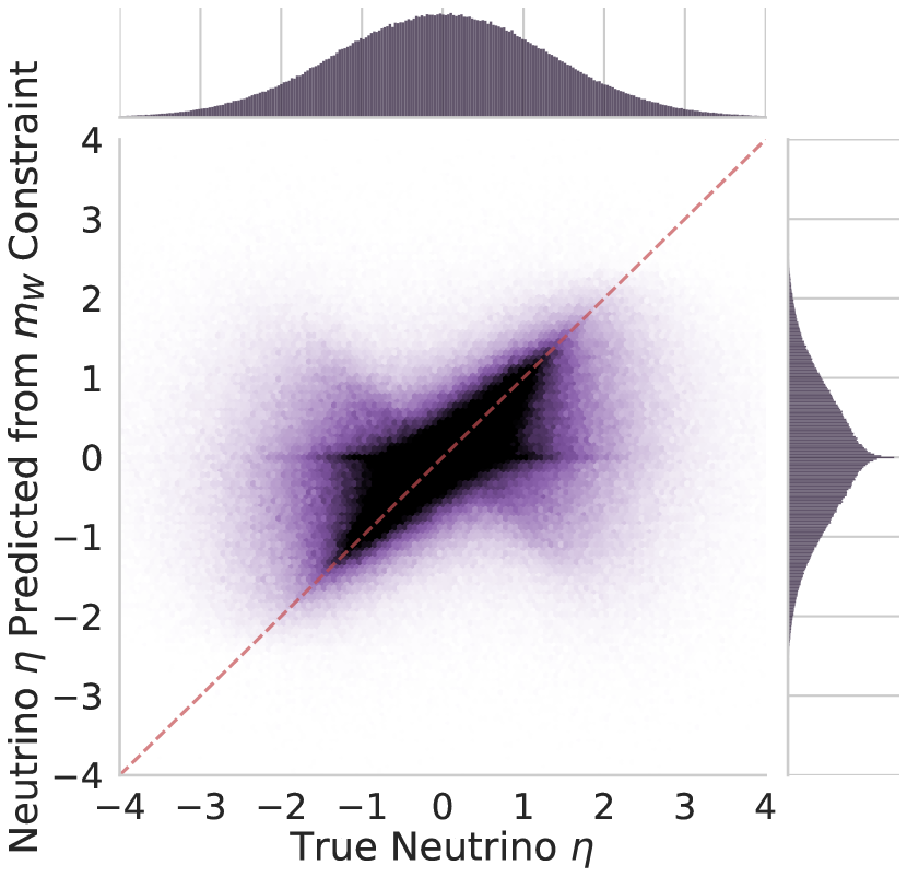
(a)

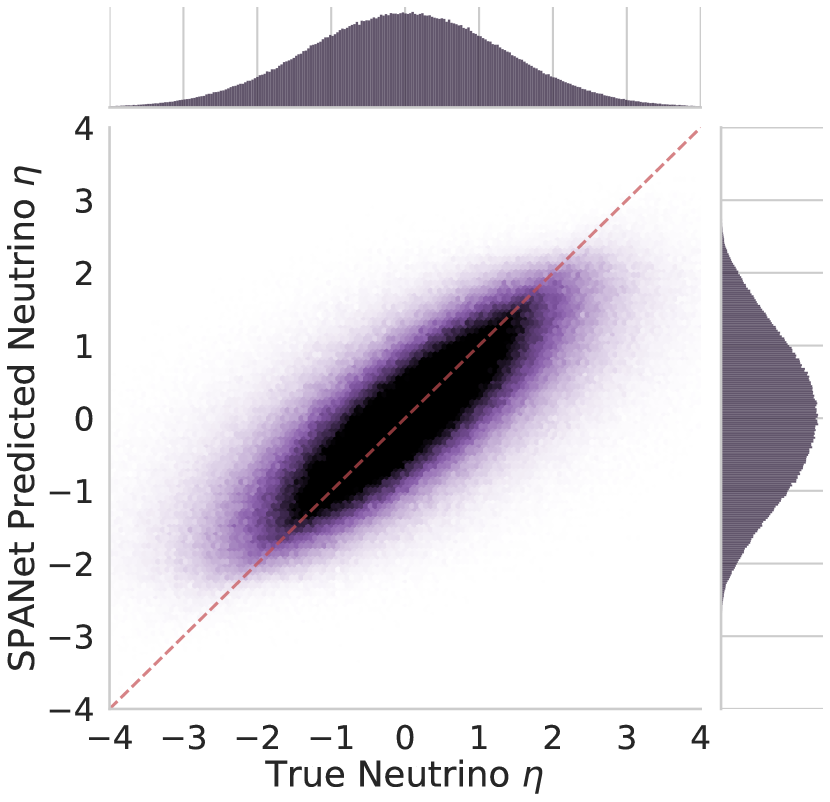
(b)

Figure 2: True neutrino pseudo-rapidity ($\eta$) versus predicted values from (2(a)) the $W$-mass constraint, and (2(b)) Spa-Net.

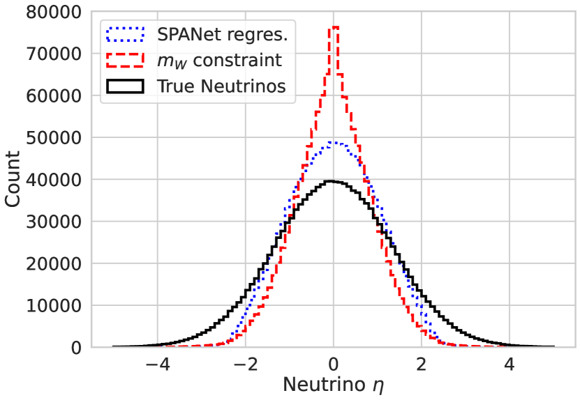
(a)

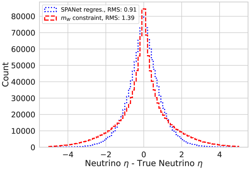
(b)

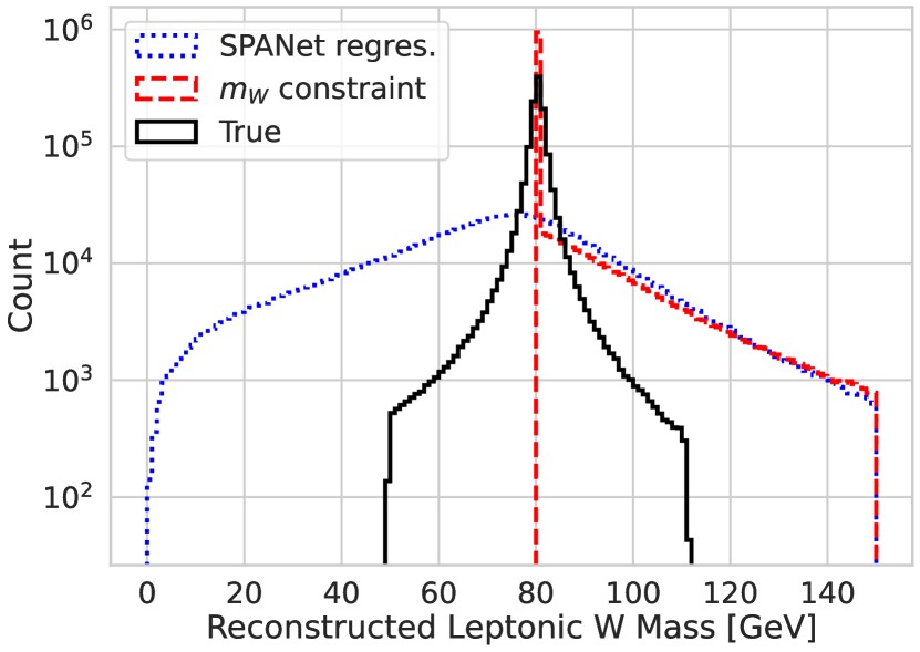
(c)

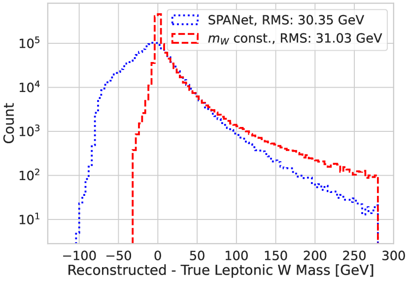
(d)

Figure 3: Comparison of the regression of neutrino pseudo-rapidity ($\eta$) by Spa-Net with the benchmark $W$ boson mass constraint method. The top row shows the neutrino $\eta$ while the bottom row shows the $W$ boson mass, with the left column the distributions of these quantities and the right column the residuals.

5.2 Particle Presence Outputs

The additional outputs described in Section 2.3 can be very useful in analysis. Figure 4(a)–4(c) shows the distributions of the assignment probability, separated by events which Spa-Net has predicted correctly or incorrectly. Similarly, Figure 4(d)–4(f) shows the distribution of the detection probability split by whether the particle was reconstructable or not. The per-particle marginal (pseudo)-probability is presented in Figure 4(g)–4(i). The KLFitter, PDNN and Spa-Net event-level likelihoods are shown in Figure 5. We note that these permutation methods only provide event-level scores for the entire assignment, and that the scores are highly overlapping with little separation between correct and incorrect. All of the Spa-Net scores show clear separation between these categories, and this separation can be used in a variety of ways, such as to remove incomplete or incorrectly matched events via direct cuts, separate different types of events into different regions, or provide direct separation power as inputs to an additional multivariate analysis. The analyses presented in Sections 8 and 9 both cut on these scores in order to remove incorrect/non-reconstructable events and improve signal-to-background ratio (S/B). In Section 7, these are used as inputs to a Boosted Decision Tree (BDT) to classify signal and background, and are found to provide a large performance gain.

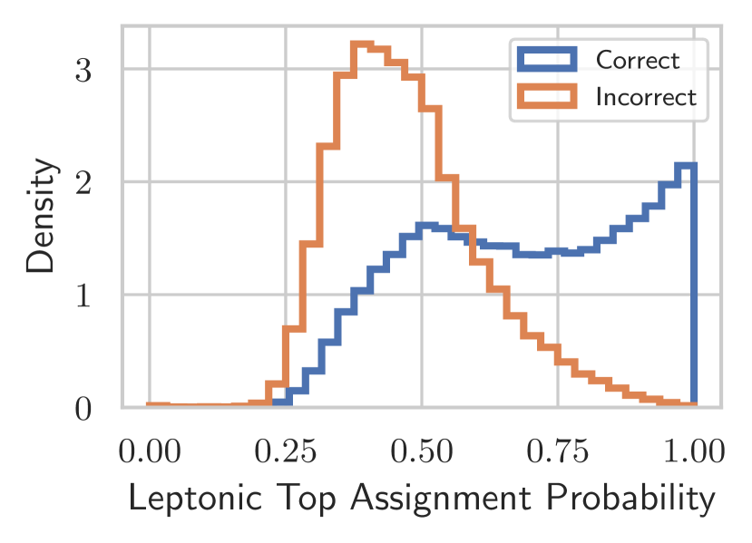
(a)

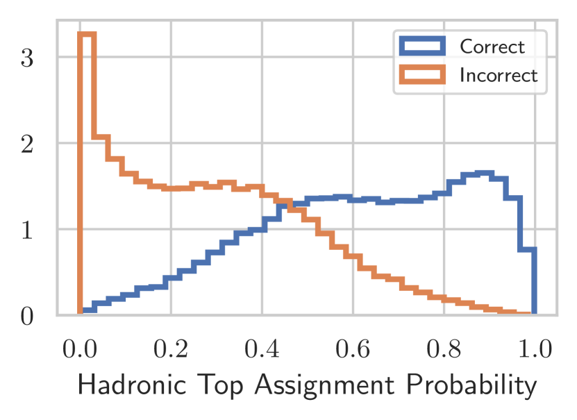
(b)

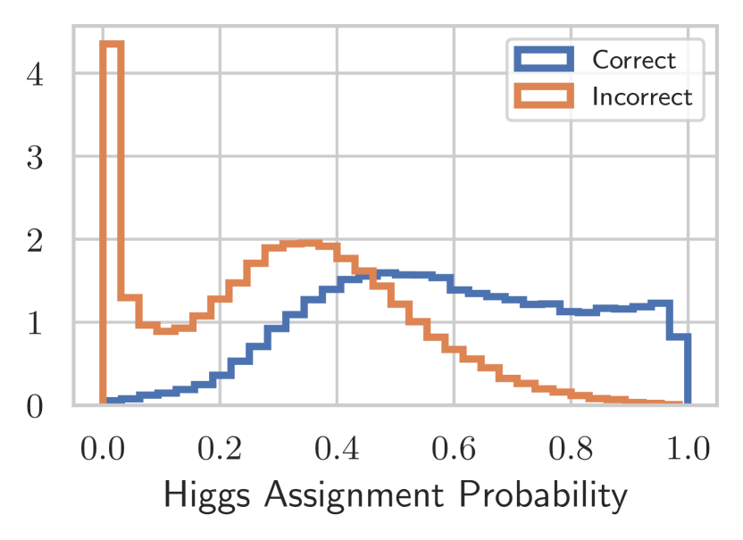
(c)

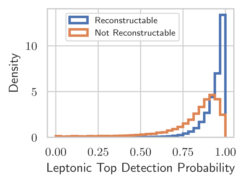
(d)

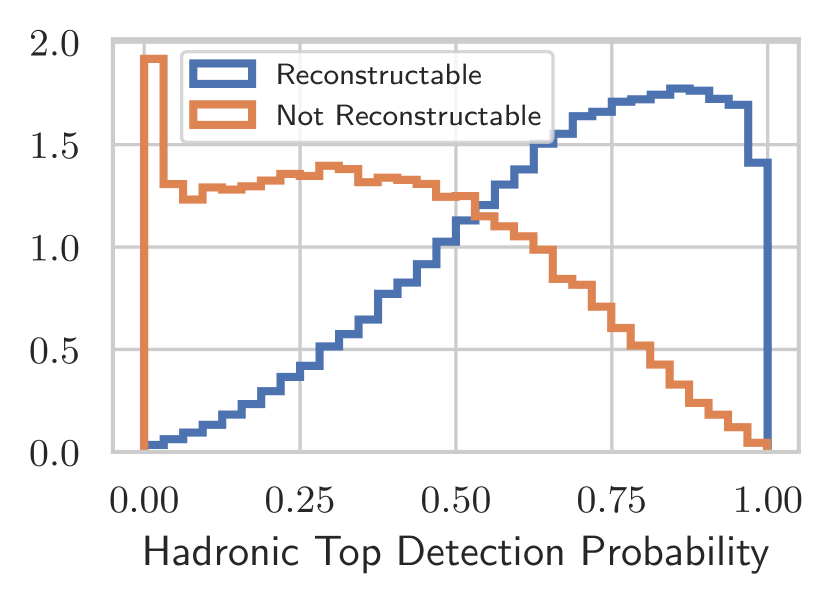
(e)

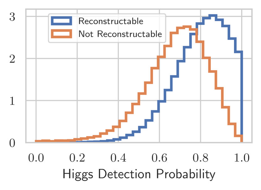
(f)

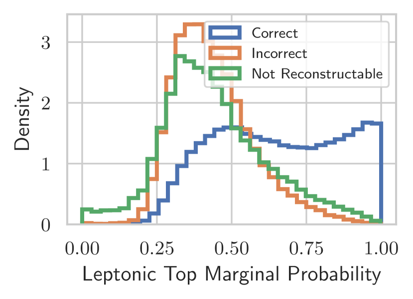
(g)

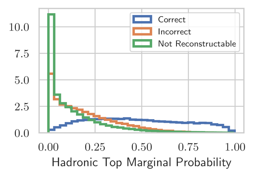
(h)

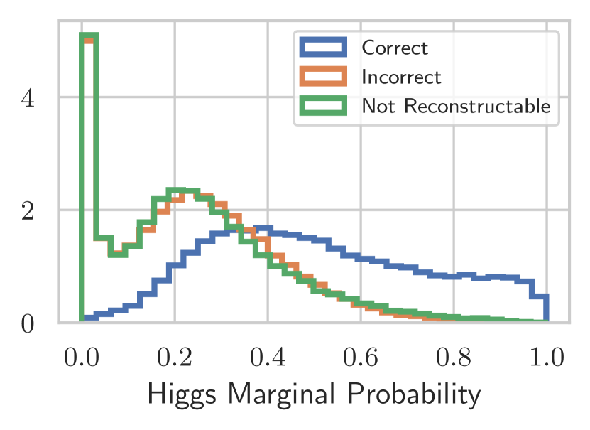
(i)

Figure 4: Spa-Net assignment (a–c), detection (d–f), and marginal (g–i) probabilities as evaluated on $t\bar{t}H$ events, grouped by whether or not Spa-Net correctly predicted the particle (a–c), by matched and unmatched events (d–f), or by correctly matched, incorrectly matched, and unmatched events (g–i). The left, middle, and right columns show the probabilities for leptonically decaying top quarks, hadronically decaying top quarks, and Higgs bosons respectively.

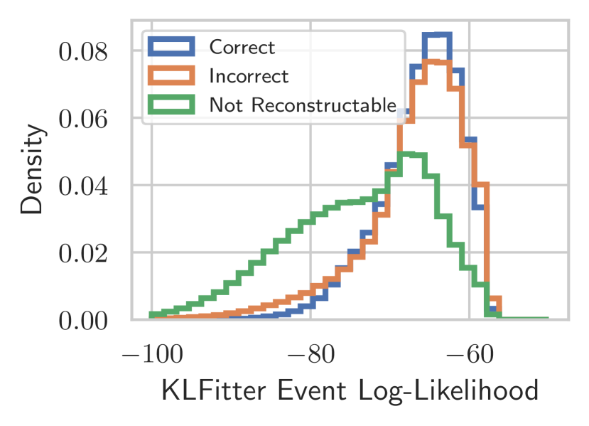
(a)

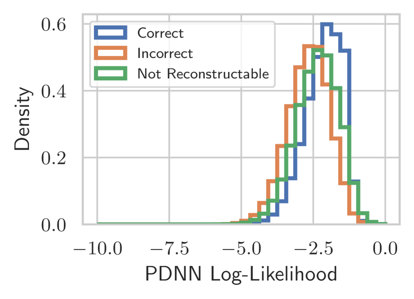
(b)

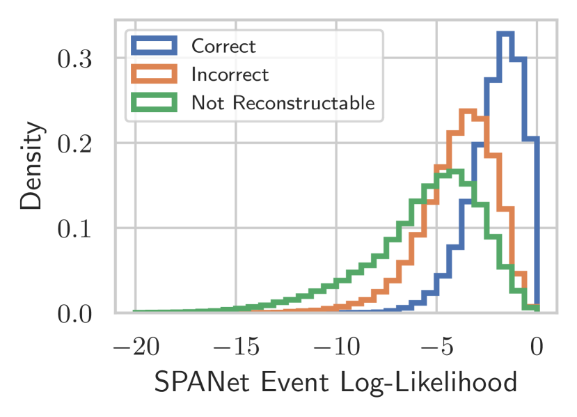
(c)

Figure 5: KLFitter, PDNN, and Spa-Net marginal event-level log-likelihood scores as evaluated on $t\bar{t}H$ events, grouped by correctly matched, incorrectly matched, and unmatched events.

5.3 Computational Overhead

Table 2 shows the average run time of jet-parton assignment on $t\bar{t}$ and $t\bar{t}H$ events. These performance tests are performed on an AMD EPYC 7502 CPU with 128 threads and an NVidia RTX 3090 GPU. Timings include all pre-initialization steps including loading the networks and data and evaluated across the testing dataset. As previously presented for the all-hadronic final states spanet2 , a few orders of magnitude speed up is observed with Spa-Net compared to the traditional methods. We also see reduced scaling between topologies for Spa-Net as $t\bar{t}$ and $t\bar{t}H$ events share very similar performance characteristics compared to the permutation methods which are much slower on $t\bar{t}H$. We also note that the PDNN achieves no significant acceleration from the GPU, as the time spent preparing the permutations dominates the computation time compared to running network inference.

	$t\bar{t}$	$t\bar{t}H$
KLFitter	24 events per second	2 events per second
PDNN CPU	2626 events per second	51 events per second
PDNN GPU	3034 events per second	101 events per second
SPANet CPU	705 events per second	852 events per second
SPANet GPU	4407 events per second	3534 events per second

Table 2: Average run time for jet-parton assignment inference from various algorithms on $t\bar{t}$ and $t\bar{t}H$ events.

6 Ablation Studies

In this section, we present several studies designed to reveal what the networks have learned.

We find that training is in general very robust, showing little dependence on details of inputs or hyperparameters. For example, training performance is unchanged within statistical uncertainties when representing particles using $\{M,p_{\mathrm{T}},\eta,\phi\}$ or $\{p_{x},p_{y},p_{z},E\}$ 4-vector representations. Reconstruction performance varies by less than 1% if the training sample with a single top mass value is replaced by that with a flat mass spectrum.

In addition, we find that the performance of the network in testing depends on the kinematic range of the training samples in a sensible way. For example, the performance of the network on independent testing events varies with the top quark pair invariant mass, reflecting the mass distribution of the training sample. Figure 6 shows the testing performance versus top quark pair mass for networks trained on the full range of masses, or only events with invariant mass less than 600 GeV. The performance at higher mass is degraded when high-mass samples are not included in the training, as the nature of the task depends on the mass, which impacts the momentum and collimation of the decay products. Furthermore, the network performance is independent of the process (SM $t\bar{t}$ or BSM $Z^{\prime}$) used to generate the training sample. The performance is reliable in the full range in which training data is present. It is noteworthy that the SM training still achieves similar performance up to around 1 TeV as the network trained on $Z^{\prime}$ events, despite having fewer events at this value, indicating that the training distribution need not be completely flat so long as some examples are present in the full range.

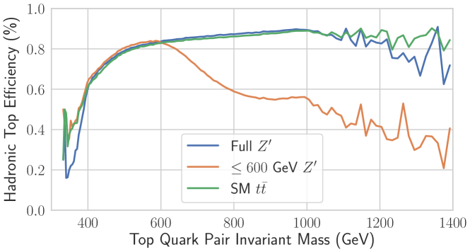
Figure 6: Performance of the networks in testing data, as measured by hadronic top reconstruction efficiency, as a function of the top quark pair invariant mass. Shown is the performance for three networks with distinct training samples: $Z^{\prime}\rightarrow t\bar{t}{}$ events with the full range of invariant masses, $Z^{\prime}\rightarrow t\bar{t}{}$ events with masses less than 600 GeV, and SM $t\bar{t}$ with the full range of invariant masses.

To evaluate if the network is learning the natural symmetries of the data, we perform two further tests. The first is to investigate the azimuthal symmetry of the events, which we evaluate by applying the network to events that are randomly rotated in the $\phi$ plane and mirrored across the beam axis, which should have no impact on the nature of the reconstruction task. Figure 7 shows the difference in marginal probability on nominal and rotated events. We observe that, in the majority of events, there is a negligible change in the outputs, though there are some events in the tails with large shifts. This demonstrates that the network approximately learns the inherent rotational and reflection symmetries of the task, without explicitly encoding this into the the network architecture.

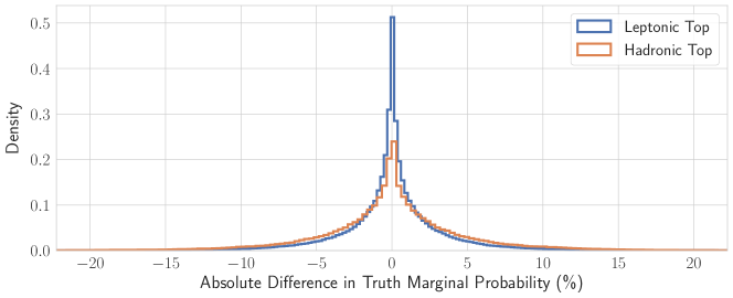
Figure 7: Difference in network output score between an event and $\phi$-rotated and / or mirrored version of the same event.

The impact of adding Lorentz invariance to the network has been evaluated by employing an explicitly invariant attention architecture which employs a matrix of relative Lorentz-covariant quantities between each pair of particles, similar to Refs. Li:2022xfc ; covariant_transformer . We follow the covariant transformer architecture covariant_transformer , and treat the $\phi$ and $\eta$ angles as Lorentz-covariant and compute the difference between these angles for all pairs of jets in the event. The remaining features are treated as Lorentz-invariant and processed normally by the attention. Figure 8(a) shows that employing the Lorentz-invariant attention improves performance for small datasets, but does not lead to higher overall performance. The Lorentz invariance does bring visible improvement in training speed as seen in Figure 8(b). After fully training both networks on various data sizes, we evaluate what batch achieved the highest validation accuracy, and we see that the invariant attention significantly reduces the number of batches needed to train the network. These observations are consistent with the findings of Refs. Li:2022xfc and covariant_transformer . The trade-off of this regime is to make each network larger and more memory intensive, as the inputs must now be represented as pairwise matrices of features instead of simple vectors. Since the overall performance in the end is the same, and since we notice that a regular network already learns to approximate this invariance, we proceed using the traditional attention architecture and this invariant network is not used for any further studies presented here.

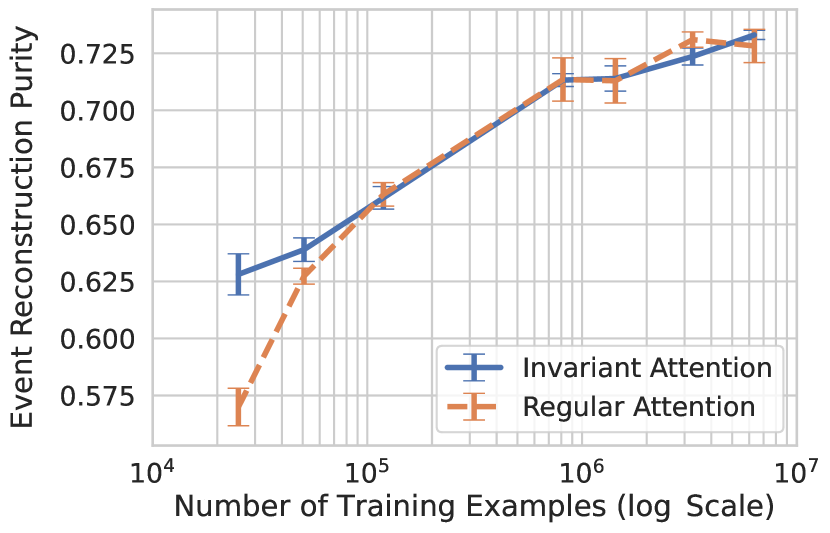
(a)

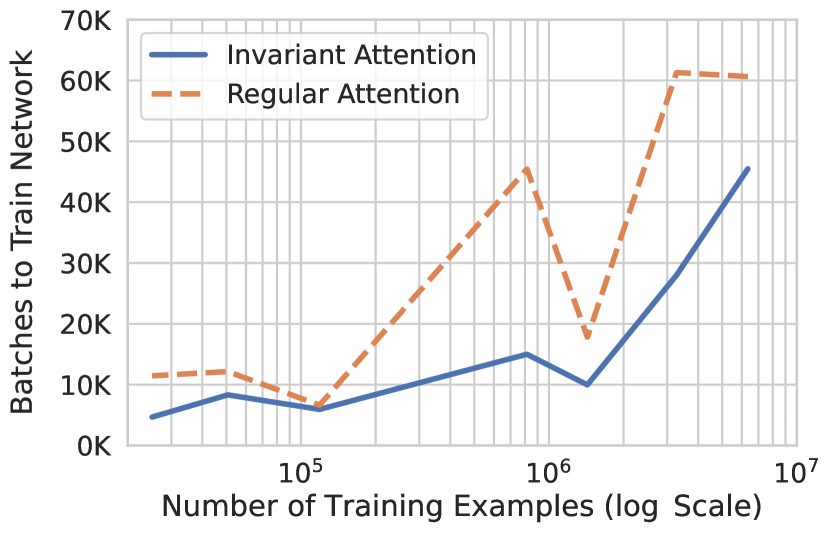
(b)

Figure 8: A comparison of (8(a)) purity and (8(b)) training speed between a regular transformer and the explicitly Lorentz-invariant transformer covariant_transformer .

7 Search for $\boldmath{t\bar{t}H(H\rightarrow b\bar{b})}$

While the previous sections have detailed the per-event performance of Spa-Net, in the following sections we demonstrate its expected impact on flagship LHC physics measurements and searches.

The central challenge of measuring the cross-section for $t\bar{t}H$ production, in which the Higgs boson follows its dominant decay mode to a pair of $b$-quarks, is separating the $t\bar{t}H$ signal from the overwhelming $t\bar{t}$+$b\bar{b}$ background. Typically, machine learning algorithms such as deep neural networks or boosted decision trees are trained to distinguish signal and background using high-level event features atlastth ; cmsttHbb . Since the key kinematic difference between the signal and background is the presence of a Higgs boson, the performance of this separation is greatly dependent on the quality of the event reconstruction, where improvements by Spa-Net can make a significant impact on the final result.

7.1 Reconstruction and Background Rejection

Event reconstruction is performed with Spa-Net, KLFitter, and a PDNN. The reconstruction efficiency for each of these methods is shown in Table 1, where it is already clear that Spa-Net outperforms both of the baseline methods.

The reconstructed quantities and likelihood or network scores are then used to train a classifier to distinguish between signal and background. A BDT is trained for each reconstruction algorithm with the same input definitions and hyperparameters using the XGBoost package xgboost . Tests using a BDT trained on lower-level information, i.e. the four-vectors of the predicted lepton and jet assignments, found weaker performance than these high-level BDTs. We also compare the performance of the BDTs to two different Spa-Net outputs that are trained to separate signal and background. The first, which we call “Spa-Net Pretraining”, is an additional output head of the primary Spa-Net network which has the objective of separating signal and background events. The second, which we call “Spa-Net Fine-tuning”, uses the same embeddings and central transformer as the former method, but the signal versus background classification head is trained in a separate second step after the initial training is complete. In this way, the network is able to first learn the optimal embedding of signal events, and utilize this embedding as the inputs to a dedicated signal vs background network.

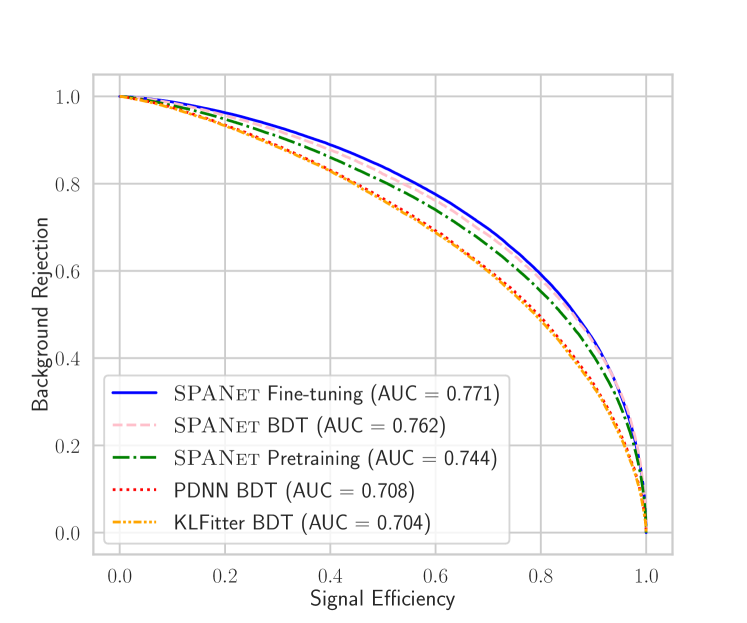
Figure 9: Receiver operating curve for networks trained to distinguish $t\bar{t}H$ from the major background $t\bar{t}{}+b\bar{b}$. Shown is signal efficiency versus background rejection for several Spa-Net based set ups as well as BDTs based on outputs of traditional reconstruction techniques; see text for details.

The receiver operating curve for the various classification networks is shown in Figure 9. The best separation performance comes from the fine-tuned Spa-Net model, as expected. The BDT with kinematic variables reconstructed with the Spa-Net jet-parton assignment (Spa-Net+BDT setup) is next, followed by the purely pre-trained model. All of these substantially outperform both the KLFitter+BDT and PDNN+BDT baselines.

7.2 Impact on sensitivity

To estimate the impact of significantly improved signal-background separation from Spa-Net reconstruction, we perform an Asimov fit to the network output distributions with the pyhf package pyhf ; pyhf_joss . The signal is normalised to the SM cross-section of 0.507 pb tthxsec and corrected for the branching fraction and selection efficiency of our sample. The dominant $t\bar{t}+b\bar{b}$ background is normalised similarly, using the cross-section calculated by MadGraph_aMC@NLO of 0.666 pb. We further multiply the background cross-sectioby a factor of 1.5, in line with measurements from ATLAS atlastth and CMS cmsttHbb that this background to be larger than SM prediction, rounded up to account also for the LO$\rightarrow$NLO cross-section enhancement. We neglect the sub-leading backgrounds. The distributions are binned according to the AutoBin feature Calvet:2296985 preferred by ATLAS in order to ensure no bias is introduced between the different methods due to the choice of binning. Results normalised to the Run 2 luminosity of 140 fb^-1 using 5 bins and assuming an uncertainty of 10% are presented in Table 3. The numbers in the parentheses in Table 3 are results for a “Run 3” analysis, normalised to 300 fb^-1 of data using 8 bins with an uncertainty assumption of 7%.

In both scenarios, the sensitivity tracks the signal-background separation performance shown in Figure 9, with Spa-Net fine-tuning achieving the greatest statistical power. Neither of the benchmark methods are able to reach the 3$\sigma$ statistical significance threshold in the Run 2 analysis, while both Spa-Net+BDT and fine-tuning reach this mark. Similarly, these methods both reach the crucial $5\sigma$ threshold normally associated with discovery, with the benchmark methods at only roughly $4\sigma$.

Table 3: Expected LHC Run 2 (3) sensitivity to $t\bar{t}H$ as measured in a parameterized detector model described in the text. Shown is the expected statistical significance of the measurement as well as expected upper limits on cross-section and signal strength using the output of classification networks trained on the products of various reconstruction algorithms. The signal strength is defined as the ratio of the Standard Model prediction to the measured cross-section.

	Signal	Upper cross	Upper signal
	significance	section limit [pb]	strength limit
KLFitter BDT	2.4$\sigma$ (4.1$\sigma$)	0.426 (0.248)	0.840 (0.489)
PDNN BDT	2.4$\sigma$ (4.1$\sigma$)	0.421 (0.246)	0.831 (0.486)
Spa-Net BDT	3.0$\sigma$ (5.2$\sigma$)	0.340 (0.196)	0.671 (0.387)
Spa-Net pre-training	2.7$\sigma$ (4.8$\sigma$)	0.371 (0.214)	0.732 (0.423)
Spa-Net fine-tuning	3.1$\sigma$ (5.7$\sigma$)	0.332 (0.179)	0.655 (0.353)

Spa-Net thus provides a significant expected improvement over the benchmark methods. While the full LHC analysis will require a more complete treatment, including significant systematic uncertainties due to choice of event generators, previous studies have demonstrated minimal dependence to such systematic uncertainties spanet2 .

8 Top Mass Measurement

The top quark mass $m_{t}$ is a fundamental parameter of the Standard Model that can only be determined via experimental measurement. These measurements are critical inputs to global electroweak fits ewkfit , and $m_{t}$ even has implications for the stability of the Higgs vacuum potential, which has cosmological consequences vacuum ; Andreassen:2017rzq . Precision measurements of the top quark mass are thus one of the most important pieces of the experimental program of the LHC, with the most recent results reaching sub-GeV precision cmstopmass ; boostedtopmass ; ATLAS:2022jbw . We demonstrate in this section the improvement enabled by the use of Spa-Net in a template-based top mass extraction.

We perform a two-dimensional fit to the invariant mass distributions of the hadronic top quark and $W$ boson as reconstructed by each method, using the basic preselection described in Section 4. We further truncate the mass distributions to 120$\leq$$m_{t}$$\leq$230 GeV and 40$\leq$$m_{W}$$\leq$120 GeV. The fraction of events with correct or incorrect predictions for the top quark jets has a strong impact on the resolution with which the mass can be extracted. Better reconstruction should thus improve the overall sensitivity to the top quark mass.

Incorporation of the $W$-mass information in the 2D fit allows for a simultaneous constraint on the jet energy scale uncertainty, often a leading contribution to the total uncertainty, by also fitting a global jet scale factor (JSF) to be applied to the $p_{\mathrm{T}}$ of each jet. Further, events that do not contain a fully reconstructable top quark are removed by cutting on the various scores from each method. KLFitter events are required to have a log-likelihood score $>$$-70$, PDNN events must have a network score of $>$0.12, and Spa-Net events must have a marginal probability of $>$0.23, optimized in each case to minimize the uncertainty on the extracted top mass. We additionally compare each method to an idealized “perfect” reconstruction method, in which all unmatched events are removed and the truth-matched reconstruction is used for all events. The perfect-matched method provides an indication of the hypothetical limit of improvement achievable through better event reconstruction. In all cases, we neglect background from other processes, since these backgrounds tend to be on the order of a few percent ATLAS:2019hxz , and would be further suppressed by the network score cuts.

The top quark mass and JSF are extracted using a template fit from Monte Carlo samples described in Section 4, which have top quark masses in 1 GeV intervals between 170 and 176 GeV. Templates are constructed for varying mass and JSF hypotheses for both the top and $W$ boson mass distributions. These templates are built separately for each of the correct, incorrect and unmatched event categories as the sum of a Gaussian and a Landau distribution, with five free parameters: the mean $\mu$ and the width $\sigma$ of each as well as the relative fraction $f$. We found an approximately linear relation between the template parameters as a function of the top quark mass and jet scale factor, allowing for linear interpolation between the mass points. Finally, we validate the mass extracted by a template fit in hypothetical similar experiments and find a small bias, for which we derive a correction.

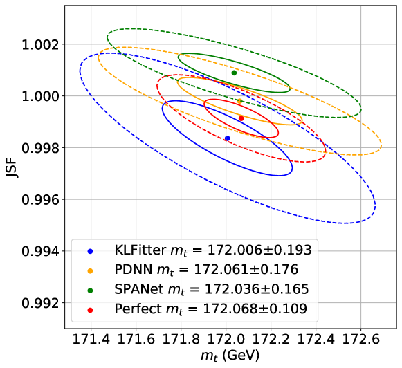
Figure 10: Expected best-fit top quark mass ($m_{t}$) and jet scale factor (JSF) from a template-based Asimov fit based on a variety of reconstruction techniques including an idealized perfect reconstruction; see text for details. Also shown are $1\sigma$ (solid) and $3\sigma$ (dashed) uncertainty ellipses.

The impact of various reconstruction techniques can be best measured by the resulting uncertainty on the top quark mass and JSF. Figure 10 shows the expected uncertainty ellipses for a dataset with luminosity of 140 fb^-1 and assuming a JSF variation of $\pm 4\%$. The final uncertainty on the top mass is $0.193$ GeV for KLFitter, $0.176$ GeV for PDNN, and $0.165$ GeV for Spa-Net. This indicates a 15% improvement in top quark mass uncertainty when using Spa-Net compared to the benchmark methods. The idealized reconstruction technique achieves an uncertainty of $0.109$ GeV, demonstrating how much room for improvement remains. The dominant contribution to the gap between the perfect and Spa-Net reconstruction comes from the perfect removal of all partial events.

9 Search for $\boldmath{Z^{\prime}\rightarrow t\bar{t}}$

Many BSM theories hypothesise additional heavy particles which may decay to $t\bar{t}$ pairs, such as heavy Higgs bosons or new gauge bosons ($Z^{\prime}$). We investigate a generic search for such a $Z^{\prime}$ particle, for which accurate reconstruction of the $t\bar{t}$ mass peak over the SM background plays a crucial role. We compare the performance of the benchmark reconstruction methods to that of various Spa-Net configurations by assessing the ability to discover a $Z^{\prime}$ signal.

An important aspect is the selection of training data, due to the unknown mass of the $Z^{\prime}$, which strongly affects the kinematics of the $t\bar{t}$ system. To avoid introducing bias into the network, the training sample is devised to be approximately flat in $m_{t\bar{t}}$, as described in Section 4. The network training was otherwise identical to that described for the SM $t\bar{t}$ network, and performance on SM $t\bar{t}$ events was approximately the same in the mass range covered by both samples.

The basic $t\bar{t}$ selection described in Section 4 is applied, and all events are reconstructed as described earlier in order to calculate the $t\bar{t}$ invariant mass, $m_{t\bar{t}}$. The mass resolution of a hypothetical resonance can often be improved by removing poorly- or partially-reconstructed events. In the context of the algorithms under comparison, this corresponds to a requirement on the KLFitter likelihood or network output scores. The threshold is chosen to optimize each algorithm, leading to a significant reduction of the SM $t\bar{t}$ background when using the PDNN and Spa-Net. More details on these cuts and the effect on the background distributions are shown in Appendix C.

9.1 Impact on sensitivity

We use the pyhf pyhf ; pyhf_joss package to extract the $Z^{\prime}$ signal and assess statistical sensitivity.

The expected results for a Run 2 analysis, normalised to 140 fb^-1 with 20 GeV bins and an uncertainty of 10%, are shown in Table 4. The discovery significance is improved by Spa-Net compared to the benchmark methods for all masses considered. For example, for a $Z^{\prime}$ of mass 700 GeV the limit improves from $1.63\sigma$ using KLFitter to $3.06\sigma$ using Spa-Net.

The expected sensitivity in a Run 3 dataset with the integrated luminosity of 300 fb^-1 is computed with an optimistic systematic uncertainty of 5% as also shown in Table 4. For all the three benchmark signals, discovery significance exceeds $5\sigma$ using Spa-Net, while for the baseline methods only the high mass point for the PDNN reaches this threshold. At a $Z^{\prime}$ mass of 500 GeV, KLFitter does not reach the $3\sigma$ evidence threshold, while Spa-Net is able to make a discovery. Interestingly, the neutrino regression does not lead to an improvement on the final sensitivity, despite showing improved resolution compared to the baseline mass constraint method. This is due to the effect on the background shape, which similarly improves in this case.

Improved reconstruction with Spa-Net can therefore greatly boost particle discovery potential. This finding should extend to other hypothetical resonances such as heavy Higgs bosons, $W^{\prime}$ bosons, or SUSY particles as well as non-$t\bar{t}$ final states such as di-Higgs, di-boson, $tb$ or any other in which reconstruction is crucial and challenging.

Table 4: Expected global significance for a $Z^{\prime}$ signal with an integrated luminosity of 140 (300) fb^-1, for several choices of $Z^{\prime}$ mass and reconstruction algorithms.

	KLFitter	PDNN	Spa-Net	Spa-Net w/ $\eta^{\nu}$
$m_{Z^{\prime}}=$ 500 GeV	1.2$\sigma$ (2.5$\sigma$)	1.8$\sigma$ (3.5$\sigma$)	2.8$\sigma$ (5.5$\sigma$)	2.7$\sigma$ (5.4$\sigma$)
$m_{Z^{\prime}}=$ 700 GeV	1.6$\sigma$ (3.3$\sigma$)	2.5$\sigma$ (4.9$\sigma$)	3.1$\sigma$ (6.1$\sigma$)	2.9$\sigma$ (5.7$\sigma$)
$m_{Z^{\prime}}=$ 900 GeV	1.9$\sigma$ (3.9$\sigma$)	2.8$\sigma$ (5.5$\sigma$)	4.3$\sigma$ (8.5$\sigma$)	4.1$\sigma$ (8.2$\sigma$)

10 Conclusions

This paper describes significant extensions and improvements to Spa-Net, a complete package for event reconstruction and classification for high energy physics experiments. We have demonstrated the application of our method to three flagship LHC physics measurements or searches, covering the full breadth of the LHC program; a precision measurement of a crucial SM parameter, a search for a rare SM process, and a search for a hypothetical new particle. In each case, use of Spa-Net provides large improvements over benchmark methods. We have further presented studies exploring what the networks learn, demonstrating a remarkable ability to learn the inherent symmetries of the data and a strong robustness to training conditions. Spa-Net is the most efficient, high performing method for event reconstruction to date, and holds great promise for helping unlock the power of the LHC dataset.

Our code is available at Ref. codebase .

11 Acknowledgments

This paper is dedicated to Megan Remillard. We would like to thank Ta-Wei Ho for assistance in generating some of the samples used in this paper. DW and MF are supported by DOE grant DE-SC0009920. The work of AS and PB in part supported by ARO grant 76649-CS to PB. HO and YL are supported by NSFC under contract No.12075060, and SCH is supported by NSF under Grant No. 2110963.

Appendix A Flat top quark and $Z^{\prime}$ mass samples

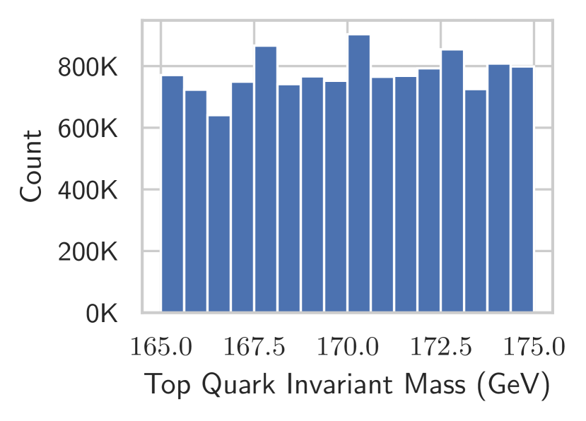
(a)

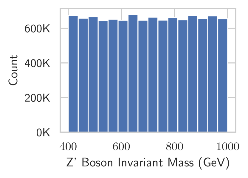
(b)

Figure 11: Distribution of top quark pair invariant mass in training samples used for (a) top quark mass measurement and (b) search for a $Z^{\prime}$ boson.

Appendix B BDT inputs for the $t\bar{t}H$ analysis

Variable	Definition
General kinematic variables
$\Delta R^{\mathrm{avg}}_{bb}$	Average $\Delta R$ for all $b$-jet pairs
$\Delta R_{bb}^{\mathrm{max}~{}p_{\mathrm{T}}}$	$\Delta R$ between the two $b$-jets with the largest vector sum $p_{\mathrm{T}}$
$\Delta\eta_{jj}^{\mathrm{max}}$	Maximum $\Delta\eta$ between any jet pairs
$H_{\mathrm{T}}^{\mathrm{had}}$	Scalar sum of jet $p_{\mathrm{T}}$
$m_{bb}^{\mathrm{min}~{}\Delta R}$	Mass of two $b$-jets with the smallest $\Delta R$
$m_{\mathrm{jj}}^{\mathrm{min}~{}\Delta R}$	Mass of any jet pair with the smallest $\Delta R$
$N_{bb}^{\mathrm{Higgs~{}30}}$	Number of $b$-jet pairs with invariant mass within 30 GeV of the Higgs mass
$\Delta R_{l,bb}^{\mathrm{min}}$	Smallest $\Delta R$ between the lepton and the combination of the two b-jets
Variables with Higgs boson and top quark reconstruction
$m_{bb}^{\text{Higgs}}$	Mass of the Higgs boson candidate
$m_{{H}\!,b_{\text{lep top}}}$	Mass of the Higgs boson candidate and $b$-jet from leptonic top quark candidate
$\Delta R^{\text{Higgs}}_{bb}$	$\Delta R$ between $b$-jets from the Higgs boson candidate
$\Delta R_{H\!,t\bar{t}}$	$\Delta R$ between Higgs boson candidate and $t\bar{t}$ candidate system
$\Delta R_{H\!,\text{leptop}}$	$\Delta R$ between Higgs boson candidate and leptonic top quark candidate
$\Delta R_{H\!,b_{\text{hadtop}}}$	$\Delta R$ between Higgs boson candidate and $b$-jet from hadronic top candidate decay
Scores from jet-parton assignment
LHD	Log-likelihood discriminant from the KLFitter
$A_{\mathrm{PDNN}}$	Assignment score from Permutation DNN
$A_{\mathrm{higgs}}$	Assignment probability of Higgs boson target from Spa-Net
$D_{\mathrm{higgs}}$	Detection probability of Higgs boson target from Spa-Net
$M_{\mathrm{higgs}}$	Marginal probability of Higgs boson target from Spa-Net
$E_{\mathrm{higgs}}$	Assignment entropy of Higgs boson target from Spa-Net
$A_{\mathrm{leptop}}$	Assignment probability of leptonic top quark candidate from Spa-Net
$D_{\mathrm{leptop}}$	Detection probability of leptonic top quark candidate from Spa-Net
$M_{\mathrm{leptop}}$	Marginal probability of leptonic top quark candidate from Spa-Net
$E_{\mathrm{leptop}}$	Assignment entropy of leptonic top quark candidate from Spa-Net
$A_{\mathrm{hadtop}}$	Assignment probability of hadronic top quark candidate from Spa-Net
$D_{\mathrm{hadtop}}$	Detection probability of hadronic top quark candidate from Spa-Net
$M_{\mathrm{hadtop}}$	Marginal probability of hadronic top quark candidate from Spa-Net
$E_{\mathrm{hadtop}}$	Assignment entropy of hadronic top quark candidate from Spa-Net

Table 5: Input variables to the classification BDT in our $t\bar{t}H$ analysis. Only the score(s) from one jet-assignment algorithm under consideration, i.e. KLFitter, PDNN, or Spa-Net, is used in the BDT and limit setting.

Appendix C Quality Cuts for the $Z^{\prime}$ analysis

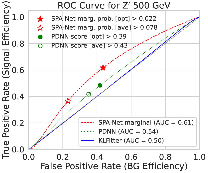
(a)

(b)

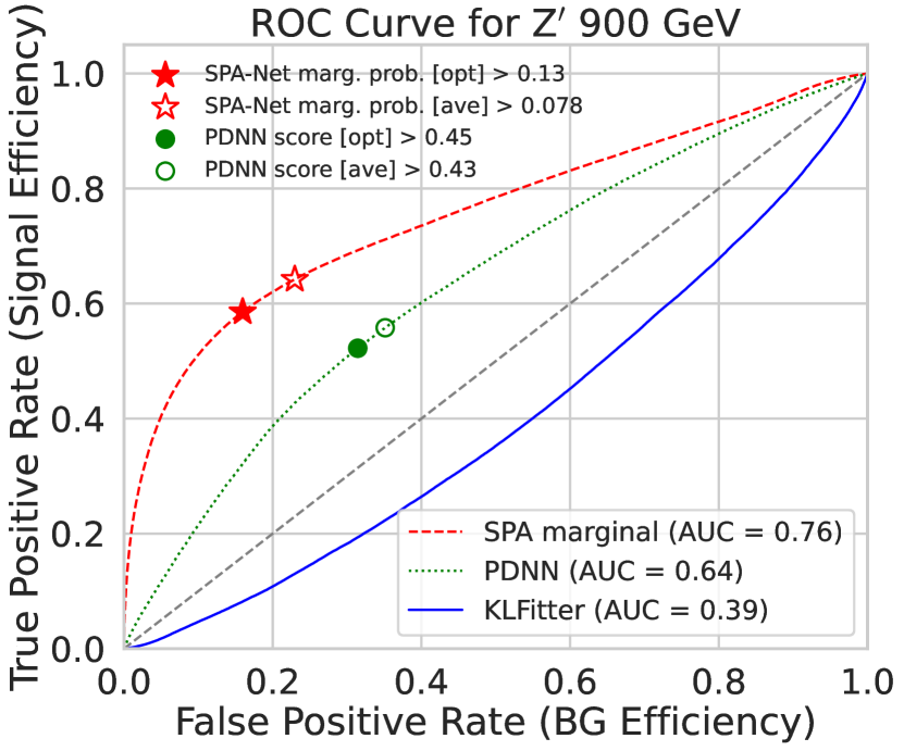
(c)

Figure 12: Receiver operating curves presented for the KLFitter likelihood, PDNN score and Spa-Net marginal probability for 500 GeV (a), 700 GeV (b) and 900 GeV (c) signal benchmarks. The optimal threshold for each signal (solid markers) and mean of the three optimal thresholds (open markers) are shown.

In typical $Z^{\prime}$ searches ZprimeATLAS ; ZprimeCMS , it is usual to apply a quality cut on the reconstruction algorithm, such as by eliminating events below a given threshold in the KLFitter likelihood or network output scores. By removing a large number of partial events or those with incorrect assignments, the mass resolution can be further improved. We tune this cut for each method to find optimal S/B for each mass point and chose the average of the optimal thresholds across the three considered mass points to be applied in our analysis. Figure 12 shows the receiver operating curve for this scan, with the optimal point for each mass denoted by a filled red star (green circle) for Spa-Net (PDNN) and the selected cut value denoted by an unfilled marker. It is found that the KLFitter likelihood actually has no impact for $Z^{\prime}$ of mass 500 GeV and actually removes more signal than the background for the 700 and 900 GeV benchmarks. Thus, we do not apply a cut on the KLFitter likelihood in our analysis. These cuts lead to a significant reduction of the SM $t\bar{t}$ background when using the PDNN and Spa-Net.

C.1 Mass Sculpting

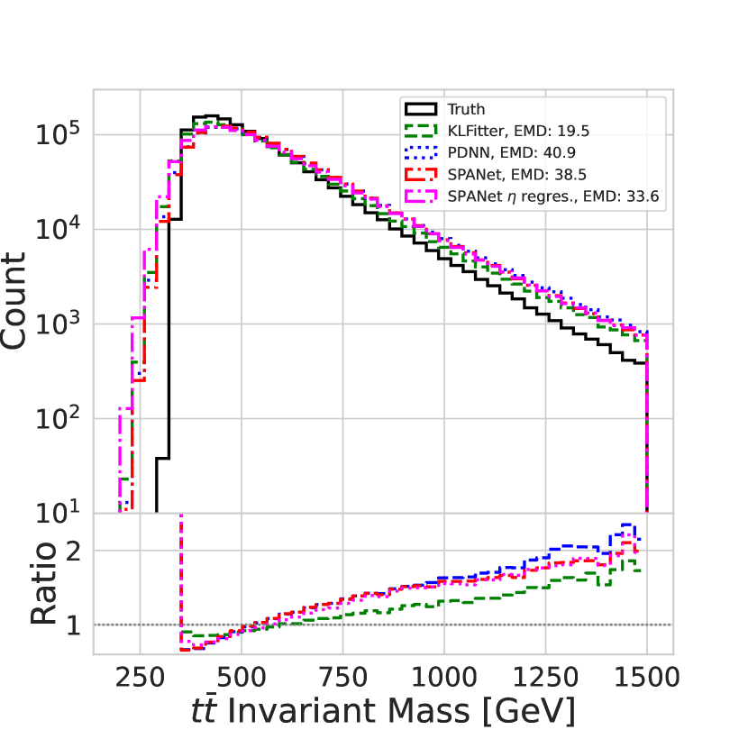
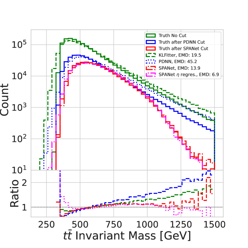
Figure 13: Invariant mass of the $t\bar{t}$ system for various jet-parton assignment algorithms without applying any score cut (left) and applying optimized score cut (right).

Another important consideration in $Z^{\prime}$ analyses is the sculpting of the background distributions induced by the reconstruction method. To assess this, Figure 13 shows the $t\bar{t}$ invariant mass distributions for each method compared to the truth distribution. The numbers in the legend are the Earth Movers Distance (EMD) metric, a measure of the difference between the truth and reconstructed distributions. Figure 13 (left) shows the distributions before the quality cuts, and demonstrate that each method has a degree of sculpting towards lower masses, with KLFitter sculpting the least and PDNN the most. Figure 13 (right) shows the same distributions for each method after the quality cuts, with this time a different truth distribution per method as each contains a different set of events. The sculpting is still visible when using the PDNN, with the EMD slightly increased, suggesting slightly increased sculpting. In comparison, the Spa-Net, the invariant mass distributions both with and without the neutrino $\eta$ regression is almost compatible with the truth distribution across the full mass range. The $\eta$ regression leads to a slightly reduced EMD indicating reduced sculpting.

References

- \bibcommenthead
- (1) Snyder, S.S.: Measurement of the Top Quark Mass at D0. PhD thesis, SUNY, Stony Brook (1995). https://doi.org/10.2172/1422822
- (2) Erdmann, J., Guindon, S., Kroeninger, K., Lemmer, B., Nackenhorst, O., Quadt, A., Stolte, P.: A likelihood-based reconstruction algorithm for top-quark pairs and the KLFitter framework. Nucl. Instrum. Meth. A 748, 18–25 (2014). https://doi.org/10.1016/j.nima.2014.02.029
- (3) Fenton, M.J., Shmakov, A., Ho, T.-W., Hsu, S.-C., Whiteson, D., Baldi, P.: Permutationless many-jet event reconstruction with symmetry preserving attention networks. Phys. Rev. D 105(11), 112008 (2022). https://doi.org/10.1103/PhysRevD.105.112008
- (4) Shmakov, A., Fenton, M.J., Ho, T.-W., Hsu, S.-C., Whiteson, D., Baldi, P.: SPANet: Generalized permutationless set assignment for particle physics using symmetry preserving attention. SciPost Phys. 12, 178 (2022). https://doi.org/10.21468/SciPostPhys.12.5.178
- (5) Workman, R.L., Others: Review of Particle Physics. PTEP 2022, 083–01 (2022). Chap. 49. https://doi.org/10.1093/ptep/ptac097
- (6) Erdmann, J., Kallage, T., Kröninger, K., Nackenhorst, O.: From the bottom to the top—reconstruction of events with deep learning. JINST 14(11), 11015 (2019). https://doi.org/10.1088/1748-0221/14/11/P11015
- (7) ATLAS Collaboration: Measurements of normalized differential cross sections for production in pp collisions at TeV using the ATLAS detector. Phys. Rev. D 90(7), 072004 (2014). https://doi.org/10.1103/PhysRevD.90.072004
- (8) ATLAS Collaboration: Measurement of the top-quark mass in the fully hadronic decay channel from ATLAS data at . Eur. Phys. J. C 75(4), 158 (2015) arXiv:1409.0832 [hep-ex]. https://doi.org/10.1140/epjc/s10052-015-3373-1
- (9) ATLAS Collaboration: Measurements of spin correlation in top-antitop quark events from proton-proton collisions at TeV using the ATLAS detector. Phys. Rev. D 90(11), 112016 (2014) arXiv:1407.4314 [hep-ex]. https://doi.org/10.1103/PhysRevD.90.112016
- (10) ATLAS Collaboration: Search for the Standard Model Higgs boson produced in association with top quarks and decaying into in pp collisions at = 8 TeV with the ATLAS detector. Eur. Phys. J. C 75(7), 349 (2015). https://doi.org/10.1140/epjc/s10052-015-3543-1
- (11) ATLAS Collaboration: Measurements of top-quark pair differential and double-differential cross-sections in the +jets channel with collisions at TeV using the ATLAS detector. Eur. Phys. J. C 79(12), 1028 (2019) arXiv:1908.07305 [hep-ex]. https://doi.org/10.1140/epjc/s10052-019-7525-6. [Erratum: Eur.Phys.J.C 80, 1092 (2020)]
- (12) ATLAS Collaboration: Measurement of the charge asymmetry in top-quark pair production in association with a photon with the ATLAS experiment. Phys. Lett. B 843, 137848 (2023). https://doi.org/10.1016/j.physletb.2023.137848
- (13) CMS Collaboration: Measurement of the top quark forward-backward production asymmetry and the anomalous chromoelectric and chromomagnetic moments in pp collisions at = 13 TeV. JHEP 06, 146 (2020). https://doi.org/10.1007/JHEP06(2020)146
- (14) CMS & ATLAS Collaborations: Combination of the W boson polarization measurements in top quark decays using ATLAS and CMS data at 8 TeV. JHEP 08(08), 051 (2020) arXiv:2005.03799 [hep-ex]. https://doi.org/10.1007/JHEP08(2020)051
- (15) CMS & ATLAS Collaborations: Combination of inclusive and differential charge asymmetry measurements using ATLAS and CMS data at and 8 TeV. JHEP 04, 033 (2018) arXiv:1709.05327 [hep-ex]. https://doi.org/10.1007/JHEP04(2018)033
- (16) https://github.com/KLFitter/KLFitter
- (17) Ehrke, L., Raine, J.A., Zoch, K., Guth, M., Golling, T.: Topological reconstruction of particle physics processes using graph neural networks. Phys. Rev. D 107(11), 116019 (2023). https://doi.org/10.1103/PhysRevD.107.116019
- (18) Alwall, J., Frederix, R., Frixione, S., Hirschi, V., Maltoni, F., Mattelaer, O., Shao, H.-S., Stelzer, T., Torrielli, P., Zaro, M.: The automated computation of tree-level and next-to-leading order differential cross sections, and their matching to parton shower simulations. JHEP 07, 079 (2014). https://doi.org/10.1007/JHEP07(2014)079
- (19) Sjöstrand, T., Ask, S., Christiansen, J.R., Corke, R., Desai, N., Ilten, P., Mrenna, S., Prestel, S., Rasmussen, C.O., Skands, P.Z.: An introduction to PYTHIA 8.2. Comput. Phys. Commun. 191, 159–177 (2015). https://doi.org/10.1016/j.cpc.2015.01.024
- (20) de Favereau, J., Delaere, C., Demin, P., Giammanco, A., Lemaître, V., Mertens, A., Selvaggi, M.: DELPHES 3, A modular framework for fast simulation of a generic collider experiment. JHEP 02, 057 (2014). https://doi.org/10.1007/JHEP02(2014)057
- (21) Cacciari, M., Salam, G.P., Soyez, G.: The anti- jet clustering algorithm. JHEP 04, 063 (2008). https://doi.org/10.1088/1126-6708/2008/04/063
- (22) ATLAS Collaboration: Measurement of Higgs boson decay into -quarks in associated production with a top-quark pair in collisions at TeV with the ATLAS detector. JHEP 06, 097 (2022). https://doi.org/10.1007/JHEP06(2022)097
- (23) Fuks, B., Ruiz, R.: A comprehensive framework for studying W′ and Z′ bosons at hadron colliders with automated jet veto resummation. JHEP 32, 5 (2017). https://doi.org/10.1007/JHEP05(2017)032
- (24) Leigh, M., Raine, J.A., Zoch, K., Golling, T.: -flows: Conditional neutrino regression. SciPost Phys. 14(6), 159 (2023). https://doi.org/10.21468/SciPostPhys.14.6.159
- (25) Raine, J.A., Leigh, M., Zoch, K., Golling, T.: -Flows: Fast and improved neutrino reconstruction in multi-neutrino final states with conditional normalizing flows (2023) arXiv:2307.02405 [hep-ph]
- (26) Li, C., Qu, H., Qian, S., Meng, Q., Gong, S., Zhang, J., Liu, T.-Y., Li, Q.: Does Lorentz-symmetric design boost network performance in jet physics? (2022) arXiv:2208.07814 [hep-ph]
- (27) Qiu, S., Han, S., Ju, X., Nachman, B., Wang, H.: Holistic approach to predicting top quark kinematic properties with the covariant particle transformer. Phys. Rev. D 107, 114029 (2023). https://doi.org/10.1103/PhysRevD.107.114029
- (28) ATLAS Collaboration: Measurement of Higgs boson decay into -quarks in associated production with a top-quark pair in collisions at TeV with the ATLAS detector. JHEP 06, 097 (2022). https://doi.org/10.1007/JHEP06(2022)097
- (29) CMS Collaboration: Measurement of the and production rates in the decay channel with of proton-proton collision data at . CMS Note, CMS-PAS-HIG-19-011 (2023)
- (30) Chen, T., Guestrin, C.: XGBoost: A scalable tree boosting system. In: Proceedings of the 22nd ACM SIGKDD International Conference on Knowledge Discovery and Data Mining. KDD ’16, pp. 785–794. ACM, New York, NY, USA (2016). https://doi.org/10.1145/2939672.2939785
- (31) https://github.com/Alexanders101/SPANet
- (32) Heinrich, L., Feickert, M., Stark, G.: pyhf: V0.7.3. https://doi.org/10.5281/zenodo.1169739. https://github.com/scikit-hep/pyhf/releases/tag/v0.7.3. https://doi.org/10.5281/zenodo.1169739
- (33) Heinrich, L., Feickert, M., Stark, G., Cranmer, K.: pyhf: pure-python implementation of histfactory statistical models. Journal of Open Source Software 6(58), 2823 (2021). https://doi.org/10.21105/joss.02823
- (34) de Florian, D., et al.: Handbook of LHC Higgs Cross Sections: 4. Deciphering the Nature of the Higgs Sector 2/2017 (2016) arXiv:1610.07922 [hep-ph]. https://doi.org/10.23731/CYRM-2017-002
- (35) Calvet, T.P.: Search for the production of a Higgs boson in association with top quarks and decaying into a b-quark pair and b-jet identification with the ATLAS experiment at LHC. PhD thesis, Aix-Marseille University (2017). https://cds.cern.ch/record/2296985
- (36) ALEPH, CDF, D0, DELPHI, L3, OPAL, SLD, LEP Electroweak Working Group, Tevatron Electroweak Working Group, SLD Electroweak, Heavy Flavour Groups: Precision Electroweak Measurements and Constraints on the Standard Model (2010) arXiv:1012.2367 [hep-ex]
- (37) Degrassi, G., Di Vita, S., Elias-Miro, J., Espinosa, J.R., Giudice, G.F., Isidori, G., Strumia, A.: Higgs mass and vacuum stability in the Standard Model at NNLO. JHEP 08, 098 (2012). https://doi.org/10.1007/JHEP08(2012)098
- (38) Andreassen, A., Frost, W., Schwartz, M.D.: Scale Invariant Instantons and the Complete Lifetime of the Standard Model. Phys. Rev. D 97(5), 056006 (2018). https://doi.org/10.1103/PhysRevD.97.056006
- (39) CMS Collaboration: Measurement of the top quark mass using a profile likelihood approach with the lepton+jets final states in proton-proton collisions at = 13 TeV (2023) arXiv:2302.01967 [hep-ex]
- (40) CMS Collaboration: Measurement of the differential production cross section as a function of the jet mass and extraction of the top quark mass in hadronic decays of boosted top quarks. Eur. Phys. J. C 83(7), 560 (2023). https://doi.org/10.1140/epjc/s10052-023-11587-8
- (41) ATLAS Collaboration: Measurement of the top-quark mass using a leptonic invariant mass in pp collisions at = 13 TeV with the ATLAS detector. JHEP 06, 019 (2023). https://doi.org/10.1007/JHEP06(2023)019
- (42) ATLAS Collaboration: Search for heavy particles decaying into top-quark pairs using lepton-plus-jets events in proton–proton collisions at TeV with the ATLAS detector. Eur. Phys. J. C 78(7), 565 (2018). https://doi.org/10.1140/epjc/s10052-018-5995-6
- (43) CMS Collaboration: Search for resonant production in proton-proton collisions at TeV. JHEP 04, 031 (2019). https://doi.org/10.1007/JHEP04(2019)031