QuantEase: Optimization-based Quantization for Language Models

Abstract

With the rising popularity of Large Language Models (LLMs), there has been an increasing interest in compression techniques that enable their efficient deployment. This study focuses on the Post-Training Quantization (PTQ) of LLMs. Drawing from recent advances, our work introduces QuantEase, a layer-wise quantization framework where individual layers undergo separate quantization. The problem is framed as a discrete-structured non-convex optimization, prompting the development of algorithms rooted in Coordinate Descent (CD) techniques. These CD-based methods provide high-quality solutions to the complex non-convex layer-wise quantization problems. Notably, our CD-based approach features straightforward updates, relying solely on matrix and vector operations, circumventing the need for matrix inversion or decomposition. We also explore an outlier-aware variant of our approach, allowing for retaining significant weights (outliers) with complete precision. Our proposal attains state-of-the-art performance in terms of perplexity and zero-shot accuracy in empirical evaluations across various LLMs and datasets, with relative improvements up to 15% over methods such as GPTQ. Leveraging careful linear algebra optimizations, QuantEase can quantize models like Falcon-180B on a single NVIDIA A100 GPU in $\sim$3 hours. Particularly noteworthy is our outlier-aware algorithm’s capability to achieve near or sub-3-bit quantization of LLMs with an acceptable drop in accuracy, obviating the need for non-uniform quantization or grouping techniques, improving upon methods such as SpQR by up to two times in terms of perplexity.

1 Introduction

Recent years have witnessed an explosive emergence of Large Language Models (LLMs) (Devlin et al., 2018; Radford et al., 2019; Brown et al., 2020; Zhang et al., 2022; Laurençon et al., 2022; Touvron et al., 2023a, b) and their ability to solve complex language modelling tasks for settings like zero-shot or instruction fine-tuning (OpenAI, 2023; Wei et al., 2022a). Consequently, there has been increased interest to utilize LLMs for real-world use cases.

The success of LLMs can be attributed to an increase in training data size and the number of model parameters (Kaplan et al., 2020; Hoffmann et al., 2022). As a result, modern LLMs have ballooned to hundreds of billions of parameters in size  (Brown et al., 2020; Zhang et al., 2022). While the ability of these models to solve tasks is remarkable, efficiently serving them remains a formidable challenge. For instance, the GPT3 model (Brown et al., 2020) contains approximately 175 billion parameters and has a memory footprint of more than 300GB. Consequently, deploying such large models on a single contemporary GPU (such as NVIDIA A6000, A100, H100) for inference has become infeasible. Another notable challenge is increased inference latency, which can prove detrimental for practical, real-world applications (Frantar et al., 2023).

Model compression has emerged as a viable approach to tackle the critical challenges of storage footprint and inference speed for LLMs (Hoefler et al., 2021). Within the modern landscape of deep learning research, numerous techniques exist that leverage weight sparsification or quantization to compress large models (Rastegari et al., 2016; Bulat and Tzimiropoulos, 2019; Agustsson et al., 2017). Since modern LLMs take significant compute resources, time, and potentially millions of dollars to train, compression-aware re-training is generally not practicable. This makes post-training quantization (PTQ) an attractive proposition. While numerous practical PTQ algorithms have already been developed (Frantar and Alistarh, 2022; Hubara et al., 2021a; Nagel et al., 2020), it is only in the most recent past that algorithms capable of effectively and efficiently quantizing and/or sparsifying extremely large LLMs have become available. Among such methods, prominent techniques include GPTQ (Frantar et al., 2023), SpQR (Dettmers et al., 2023) and AWQ (Lin et al., 2023), among others. These methods aim to compress a 16-bit model into 3 or 4 bits while striving to maintain predictive accuracy. Despite promising progress in this realm, a discernible drop in the performance of quantized models persists compared to their unquantized counterparts. In this paper, we focus on developing a new algorithm for PTQ of network weights of LLMs.

Figure 1: Zero-Shot accuracy on the LAMBADA (Paperno et al., 2016) benchmark for 3-bit quantization. See Section 5.3 for more details on experimental setup. QuantEase  consistently outperforms methods like GPTQ and AWQ, sometimes by 15% in terms of relative improvement.

1.1 Our Approach

In this paper, we propose QuantEase - a new algorithm to obtain high-quality feasible (i.e. quantized) solutions to layerwise post-training quantization of LLMs. QuantEase leverages cyclic Coordinate Descent (CD) (Tseng, 2001). CD-type methods have traditionally been used to address statistical problems (Chang and Lin, 2011; Mazumder and Hastie, 2012; Friedman et al., 2010; Hazimeh and Mazumder, 2020; Shevade and Keerthi, 2003; Behdin et al., 2023). We show that QuantEase is a more principled optimization method when compared to methods like GPTQ, guaranteeing a non-increasing sequence of the objective value under feasibility of the initial solution. QuantEase cycles through coordinates in each layer, updating each weight such that it minimizes the objective while keeping other weights fixed. This allows for simple closed-form updates for each weight. Empirically, this results in up to 30% improvement in relative quantization error over GPTQ for 4-bit and 3-bit quantization (see Figure 2).

QuantEase’s simplicity allows it to have several advantages over other methods, while making it extremely scalable and easy to use. Unlike other methods, QuantEase does not require expensive matrix inversion or Cholesky factorization. This helps avoid numerical issues while also lowering memory requirements. QuantEase is extremely easy to implement, making it a drop-in replacement for most other methods. Remarkably, QuantEase can efficiently quantize a 66B parameter model on a single NVIDIA V100 GPU, whereas methods like GPTQ and AWQ run out of memory. QuantEase is also extremely time efficient and is able to quantize extremely large models like Falcon-180b (Penedo et al., 2023) within a few hours, where each iteration has speed that is comparable to a well-optimized implementation of GPTQ.

QuantEase’s effectiveness in achieving lower quantization error also translates to improvements on language modeling benchmarks. Experiments on several LLM model families (Laurençon et al., 2022; Zhang et al., 2022; Penedo et al., 2023) and language tasks show that QuantEase outperforms state-of-the-art uniform quantization methods such as GPTQ and AWQ in terms of perplexity and zero-shot accuracy (Paperno et al., 2016), both in the 4-bit and 3-bit regimes (see Tables 1,  2,  3 and Figures 1, 4). For the 3-bit regime, QuantEase  is especially effective for zero-shot accuracy, achieving strong relative improvements (up to 15%) over GPTQ (see Figure 1).

We also propose a variant of QuantEase to handle weight outliers. This is achieved by dividing the set of layer weights into a group of quantized weights and very few unquantized ones. We propose a block coordinate descent method based on iterative hard thresholding (Blumensath and Davies, 2009) for the outlier-aware version of our method. This version of QuantEase is able to improve upon outlier-based models such as SpQR. Particularly, we show this outlier-aware method can achieve acceptable accuracy for sub-3 bit regimes, improving upon current available methods such as SpQR by up to 2.5 times in terms of perplexity. We hope that the simplicity and effectiveness of QuantEase inspires further research in this area.

Our contributions can be summarised as follows:

1. Principled optimization - We propose QuantEase, an optimization framework for post-training quantization of LLMs based on minimizing a layerwise (least squares) reconstruction error. We propose a CD framework updating network weights one-at-a-time, avoiding memory-expensive matrix inversions/factorizations. Particularly, we make the CD updates efficient by exploiting the problem structure resulting in closed form updates for weights.

2. Outlier awareness - We also propose an outlier-aware version of our framework where a few (outlier) weights are kept unquantized. We discuss an algorithm for outlier-aware QuantEase based on block coordinate descent and iterative hard thresholding.

3. Improved accuracy - Experiments on LLMs with billions of parameters show that QuantEase outperforms recent PTQ methods such as GPTQ and AWQ in text generation and zero-shot tasks for 3 and 4-bit quantization, often by a large margin. Additional experiments show that the outlier-aware QuantEase outperforms methods such as SpQR by up to 2.5 times in terms of perplexity, in the near-3 or sub-3 bit quantization regimes.

1.2 Related Work

Recently, there has been a mounting interest in the layerwise quantization of LLMs. One prominent method for post-training quantization of LLMs is GPTQ (Frantar et al., 2023). GPTQ extends the Optimal Brain Surgeon (OBS) framework (LeCun et al., 1989; Hassibi and Stork, 1992; Frantar and Alistarh, 2022), incorporating strategies for layerwise compression (Dong et al., 2017). Empirical evaluations of GPTQ demonstrate encouraging results, revealing a marginal drop in accuracy in text generation and zero-shot benchmarks. Another avenue for achieving layer-wise quantization of LLMs is the recent work by Lin et al. (2023), referred to as AWQ. This approach centres on preserving the weights that influence activations most. GPTQ and AWQ represent two prominent foundational techniques, and we will compare our methodology against these in our numerical experiments.

It is widely acknowledged that transformer models, inclusive of LLMs, confront challenges tied to outliers when undergoing quantization to lower bit-widths (Wei et al., 2022b; Bondarenko et al., 2021; Kim et al., 2023). This predicament arises from the notable impact of extremely large or small weights on the quantization range, thereby leading to supplementary errors. As a result, specific research endeavours delve into the notion of non-uniform quantization. SqueezeLLM (Kim et al., 2023) seeks to identify and preserve outlier weights (for example, very large or small weights) that might affect the output the most, allowing for improved accuracy. Similarly, SpQR (Dettmers et al., 2023) combines GPTQ with outlier detection to achieve a lower loss of accuracy. We use SpQR as a benchmark in our experiments with outlier detection.

A long line of work discuss and study quantization methods for large neural networks from an implementation perspective, including hardware-level optimizations for low-bit calculations and inference time activation quantization, which are beyond the scope of this paper. For a more exhaustive exposition, please check Gholami et al. (2022); Wang et al. (2020); Hubara et al. (2021b); Xiao et al. (2023); Yao et al. (2022, 2023) and the references therein.

2 Background

2.1 Problem Formulation: Layerwise Quantization

A standard approach to LLM compression is layerwise compression (Dong et al., 2017), where layers are compressed/quantized one at a time. This allows the task of compressing a very large network to be broken down into compressing several smaller layers, which is more practical than simultaneously quantizing multiple layers. In this paper, we pursue a layerwise framework for quantization.

Focusing on layerwise quantization, let us consider a linear layer with some (nonlinear) activation function. Within this context, let $\boldsymbol{X}\in\mathbb{R}^{p\times n}$ represent the input matrix feeding into this particular layer, where $p$ denotes the number of input features and $n$ denotes the number of training data points fed through the network. Additionally, let $\boldsymbol{W}\in\mathbb{R}^{q\times p}$ symbolize the weights matrix corresponding to this layer, characterized by $q$ output channels.

For a given output channel $i\in[q]$, we designate the predetermined, finite set of per-channel quantization levels for this channel as $\mathcal{Q}_{i}\subseteq\mathbb{R}$. In this work, following Frantar et al. (2023), we focus on the case where the quantization levels within $\mathcal{Q}_{i}$ are uniformly spaced (We note however, that our approach can extend to quantization schemes that do not follow this assumption.). We can then formulate the layerwise quantization task as the following optimization problem:

$$\min_{\hat{\boldsymbol{W}}}f(\hat{\boldsymbol{W}}):=\|\boldsymbol{W}\boldsymbol{X}-\hat{\boldsymbol{W}}\boldsymbol{X}\|^{2}_{F}~{}~{}\text{s.t.}~{}~{}\hat{W}_{i,j}\in\mathcal{Q}_{i},(i,j)\in[q]\times[p].$$ (1)

The objective of Problem (1) captures the distance between the original pre-activation output obtained from unquantized weights ($\boldsymbol{W}\boldsymbol{X}$), and the pre-activation output stemming from quantized weights ($\hat{\boldsymbol{W}}\boldsymbol{X}$), subject to $\hat{\boldsymbol{W}}$ adhering to quantization constraints.

Notation: For $i\in[q]:=\{1,\ldots,q\}$, we define the quantization operator $q_{i}$ with respect to quantization levels $\mathcal{Q}_{i}$ as follows:

$$q_{i}(x)\in\mathop{\mathrm{argmin}}_{y\in\mathcal{Q}_{i}}~{}(x-y)^{2}.$$ (2)

For a matrix such as $\boldsymbol{A}$, $\|\boldsymbol{A}\|_{F}$ denotes its Frobenius norm. Moreover, for $i<j$, $\boldsymbol{A}_{:,i}$ and $\boldsymbol{A}_{:,i:j}$ denote the $i$-th column, and columns $i$ to $j$ of $\boldsymbol{A}$, respectively. The proofs of the main results are relegated to Appendix B.

2.2 Two Key Algorithms

2.2.1 GPTQ

As mentioned earlier, GPTQ (Frantar et al., 2023) extends the OBS-based framework of Frantar and Alistarh (2022); Hassibi and Stork (1992). GPTQ performs quantization of $\boldsymbol{W}$ one column at a time. Specifically, GPTQ starts with the initialization, $\hat{\boldsymbol{W}}\leftarrow\boldsymbol{W}$. Then, it cycles through columns $j=1,\cdots,p$ and for each $j$, it quantizes column $j$ of $\hat{\boldsymbol{W}}$. For the $j$-th column it quantizes all its entries via the updates: $\hat{{W}}_{i,j}^{+}=q_{i}(\hat{{W}}_{i,j}),~{}i\in[q].$ After updating the $j$-th column, GPTQ proceeds to update the other weights in the layer to ensure that the error in (1) does not increase too much. To make our exposition resemble that of the OBS framework, we note that GPTQ updates $\hat{\boldsymbol{{W}}}_{:,j+1:p}$ by approximately solving the least-squares problem:

$$\min_{\hat{\boldsymbol{{W}}}_{:,j:p}}\|\boldsymbol{W}\boldsymbol{X}-\hat{\boldsymbol{W}}\boldsymbol{X}\|_{F}^{2}~{}~{}~{}\text{s.t.}~{}~{}~{}\hat{\boldsymbol{W}}_{:,j}=\hat{\boldsymbol{W}}^{+}_{:,j},$$ (3)

where the constraint above implies that we are effectively optimizing over $\hat{\boldsymbol{W}}_{:j+1:p}$ (but we choose this representation following Hassibi and Stork (1992); Frantar and Alistarh (2022)). We note that in (3), the quantization constraints are dropped as otherwise, (3) would be as hard as (1) in general. Moreover, entries up to the $j$-th column i.e, $\hat{\boldsymbol{W}}_{:,1:j}$ are not updated to ensure they remained quantized. Since the OBS framework is set up to optimize a homogeneous quadratic, Frantar and Alistarh (2022); Frantar et al. (2023) reformulate Problem (3) as

$$\min_{\hat{\boldsymbol{{W}}}_{:,j:p}}\|\boldsymbol{A}+(\boldsymbol{W}_{:,j}-\hat{\boldsymbol{W}}_{:,j})\boldsymbol{X}_{j,:}+(\boldsymbol{W}_{:,j+1:p}-\hat{\boldsymbol{W}}_{:,j+1:p})\boldsymbol{X}_{j+1:p,:}\|_{F}^{2}~{}~{}~{}\text{s.t.}~{}~{}~{}\hat{\boldsymbol{W}}_{:,j}=\hat{\boldsymbol{W}}^{+}_{:,j}$$ (4)

where

$$\boldsymbol{A}=(\boldsymbol{W}_{:,1:j-1}-\hat{\boldsymbol{W}}_{:,1:j-1})\boldsymbol{X}_{1:j-1,:}.$$ (5)

Upon inspection one can see that the objective in (4) is not homogeneous quadratic, and hence does not fit into the OBS framework. Therefore, $\boldsymbol{A}$ is dropped and this problem is replaced by the formulation:

$$\min_{\hat{\boldsymbol{{W}}}_{:,j:p}}\|(\boldsymbol{W}_{:,j}-\hat{\boldsymbol{W}}_{:,j})\boldsymbol{X}_{j,:}+(\boldsymbol{W}_{:,j+1:p}-\hat{\boldsymbol{W}}_{:,j+1:p})\boldsymbol{X}_{j+1:p,:}\|_{F}^{2}~{}~{}~{}\text{s.t.}~{}~{}~{}\hat{\boldsymbol{W}}_{:,j}=\hat{\boldsymbol{W}}^{+}_{:,j}$$

$$\stackrel{{\scriptstyle(a)}}{{=}} \min_{\hat{\boldsymbol{{W}}}_{:,j:p}}\mathsf{Tr}((\boldsymbol{W}_{:,j:p}-\hat{\boldsymbol{W}}_{:,j:p})^{T}\boldsymbol{\Sigma}_{F}(\boldsymbol{W}_{:,j:p}-\hat{\boldsymbol{W}}_{:,j:p}))~{}~{}~{}\text{s.t.}~{}~{}~{}\hat{\boldsymbol{W}}_{:,j}=\hat{\boldsymbol{W}}^{+}_{:,j}$$ (6)

where $\boldsymbol{\Sigma}_{F}=\boldsymbol{X}_{j:p,:}\boldsymbol{X}_{j:p,:}^{T}$, $F$ refers to the $\{j,\cdots,p\}$ indices and $(a)$ is by $\|\boldsymbol{M}\|_{F}^{2}=\mathsf{Tr}(\boldsymbol{M}^{T}\boldsymbol{M})$ for any matrix $\boldsymbol{M}$. Therefore, after updating the $j$-th column to $\hat{\boldsymbol{W}}_{:,j}^{+}$, we can update $\hat{\boldsymbol{{W}}}_{:,j+1:p}$ by the OBS updates (we refer to Frantar et al. (2023); Frantar and Alistarh (2022) for derivation details):

$$\boldsymbol{\delta} \leftarrow-\frac{\hat{\boldsymbol{W}}_{:,j}-\hat{\boldsymbol{W}}_{:,j}^{+}}{[\boldsymbol{\Sigma}_{F}^{-1}]_{j,j}}$$ (7)

$$\hat{\boldsymbol{{W}}}_{:,j+1:p} \leftarrow\hat{\boldsymbol{{W}}}_{:,j+1:p}+\boldsymbol{\delta}[\boldsymbol{\Sigma}_{F}^{-1}]_{j,j+1:p}$$

We note that the OBS updates in (7) require the calculation of $\boldsymbol{\Sigma}^{-1}_{F}$. Therefore, using the updates in (7) can be expensive in practice. To improve efficiency, GPTQ uses a lazy-batch update scheme where at each step, only a subset (of size at most 128) of the remaining unquantized weights is updated.

2.2.2 AWQ

Similar to GPTQ, AWQ (Lin et al., 2023) uses a layerwise quantization framework. However, different from GPTQ, the main idea behind AWQ is to find a rescaling of weights that does not result in high quantization error, rather than directly minimizing the least squares criteria for layerwise reconstruction. To this end, AWQ considers the following optimization problem:

$$\min_{\boldsymbol{s}\in\mathbb{R}^{p}}\|\boldsymbol{W}\boldsymbol{X}-\boldsymbol{q}(\boldsymbol{s}\odot\boldsymbol{W})(\boldsymbol{X}\odot\boldsymbol{s}^{-1})\|_{F}^{2}$$ (8)

where $[\boldsymbol{q}(\boldsymbol{W})]_{i,j}=q_{i}(W_{i,j})$ quantizes a vector/matrix coordinate-wise, $[\boldsymbol{s}^{-1}]_{i}=s_{i}^{-1}$ is the coordinate-wise inversion and $\odot$ is the channel-wise multiplication, $[\boldsymbol{s}\odot\boldsymbol{W}]_{i,j}=s_{j}W_{i,j}$ and $[\boldsymbol{X}\odot\boldsymbol{s}^{-1}]_{i,j}=X_{i,j}/s_{i}$. In Problem (8), $\boldsymbol{s}$ is the per-channel scaling. Problem (8) is non-differentiable and non-convex and cannot be efficiently solved. Therefore, Lin et al. (2023) discuss grid search heuristics for $\boldsymbol{s}$ to find a value that does not result in high quantization error. Particularly, they set $\boldsymbol{s}=\boldsymbol{s_{\boldsymbol{X}}}^{\alpha}*{s_{\boldsymbol{W}}}^{-\beta}$ for some $\alpha,\beta\in[0,1]$, where $*$ is coordinate-wise multiplication, and $\boldsymbol{s}_{\boldsymbol{X}},\boldsymbol{s}_{\boldsymbol{W}}\in\mathbb{R}^{p}$ are per-channel averages of magnitude of $\boldsymbol{X}$ and $\boldsymbol{W}$, respectively. The values of $\alpha,\beta$ are then chosen by grid search over the interval $[0,1]$. After choosing the value of $\boldsymbol{s}$, the quantized weights are given as $\boldsymbol{s}^{-1}\odot\boldsymbol{q}(\boldsymbol{s}\odot\boldsymbol{W})$.

3 Our Proposed Method

3.1 Overview of QuantEase

Our algorithm is based on the cyclic CD method (Tseng, 2001). At every update of our CD algorithm, we minimize the objective in (1) with respect to the coordinate $\hat{W}_{i,j}$ while making sure $\hat{W}_{i,j}\in\mathcal{Q}_{i}$. At each step, we keep all other weights fixed at their current value. For $(i,j)\in[q]\times[p]$ we update $\hat{W}_{i,j}$, as follows:

$$\hat{W}_{i,j}^{+}\in\mathop{\mathrm{argmin}}_{\hat{W}_{i,j}\in\mathcal{Q}_{i}}f(\hat{W}_{1,1},\cdots,\hat{W}_{i,j},\cdots,\hat{W}_{q,p})$$ (9)

where $\hat{\boldsymbol{W}}^{+}$ is the solution after the update of coordinate $(i,j)$. In words, $\hat{W}_{i,j}^{+}$ is obtained by solving a 1D optimization problem: we minimize the 1D function $\hat{W}_{i,j}\mapsto f(\hat{\boldsymbol{W}})$ under the quantization constraint. This 1D optimization problem, despite being non-convex, can be solved to optimality in closed-form (See Section 3.2 for details). A full pass over all coordinates $(i,j)\in[q]\times[p]$ completes one iteration of the CD algorithm. QuantEase usually makes several iterations to obtain a good solution to (1).

We initialize QuantEase with the unquantized original weights of the layer. This means that $\hat{\boldsymbol{W}}$ is generally infeasible for Problem (1) (i.e., it does not fully lie on the quantization grid) till the end of the first iteration. However, from the second iteration onward, feasibility is maintained by QuantEase, while continuously decreasing $f$. This is useful because QuantEase can be terminated any time after the first iteration with a feasible solution.

It is worth mentioning that, unlike QuantEase, GPTQ does only one pass through the columns of $\hat{\boldsymbol{W}}$. Once $\hat{\boldsymbol{W}}$ is feasible (fully quantized) at the end, the OBS idea is not usable any more. Hence further iterations are not possible and so GPTQ stops there. Interestingly, QuantEase can be initialized with the $\hat{\boldsymbol{W}}$ obtained by GPTQ (or any other algorithm) and run for several iterations to optimize Problem (1) even further.

3.2 Computational Considerations for QuantEase

Closed-form updates: The efficiency of the CD method depends on how fast the update (9) can be calculated. Lemma 1 derives a closed form solution for Problem (9).

Lemma 1.

Let $\boldsymbol{\Sigma}=\boldsymbol{X}\boldsymbol{X}^{T}$. Then, $\hat{W}_{i,j}^{+}=q_{i}(\tilde{\beta})$ in (9) where

$$\tilde{\beta}=-\left[\sum_{k\neq j}\Sigma_{j,k}\hat{W}_{i,k}-(\boldsymbol{W}\boldsymbol{\Sigma})_{i,j}\right]/\Sigma_{j,j}.$$ (10)

Proof of Lemma 1 can be found in Appendix B. We note that $\tilde{\beta}$ in (10) minimizes the one-dimensional function $\hat{W}_{i,j}\mapsto f(\hat{W}_{1,1},\cdots,\hat{W}_{i,j},\cdots,\hat{W}_{q,p})$ where $\hat{W}_{i,j}$ is unconstrained (i.e., without any quantization constraint). Therefore, interestingly, Lemma 1 shows that to find the best quantized value for $\hat{W}_{i,j}$ in (9), it suffices to quantize the value that minimizes the one-dimensional function, $\hat{W}_{i,j}\mapsto f(\hat{W}_{1,1},\cdots,\hat{W}_{i,j},\cdots,\hat{W}_{q,p})$ under no quantization constraint. Since we find the minimizer per coordinate and then quantize the minimizer, this is different from quantizing the “current” weight.

Memory Footprint: The matrices, $\boldsymbol{\Sigma}$ and $\boldsymbol{W}\boldsymbol{\Sigma}$ do not change over iterations and can be stored with $p^{2}+\mathcal{O}(pq)$ memory footprint. This is specially interesting as in practice, $n\gg p,q$. QuantEase, unlike GPTQ, also does not require matrix inversion or Cholesky factorization which can be memory-inefficient (either adding up to $\mathcal{O}(p^{2})$ storage).

Parallelization over $i\in[q]$: As seen in Lemma 1, for a given $j_{0}\in[p]$, the updates of $\hat{W}_{i,j_{0}}$ are independent (for each $i$) and can be done simultaneously. Therefore, rather than updating a coordinate $\hat{W}_{i,j}$ at a time, we update a column of $\hat{W}$, that is: $\hat{W}_{:,j}$ at each update. This allows us to better make use of the problem structure (see the rank-1 update below).

Rank-1 updates: Note that in (10), we need access to terms of the form $\sum_{k\neq j}\Sigma_{j,k}\hat{W}_{i,k}$. Such terms can be refactored as:

$$\sum_{k\neq j}\Sigma_{j,k}\hat{W}_{i,k}=\sum_{k=1}^{p}\Sigma_{j,k}\hat{W}_{i,k}-\Sigma_{j,j}\hat{W}_{i,j}=\hat{\boldsymbol{W}}_{i,:}\boldsymbol{\Sigma}_{:,j}-\Sigma_{j,j}\hat{W}_{i,j}.$$

However, as noted above, we update all the rows corresponding to a given column of $\hat{\boldsymbol{W}}$ at once. Therefore, to update a column of $\hat{\boldsymbol{W}}$, we need access to the vector

$$\left(\sum_{k\neq j}\Sigma_{j,k}\hat{W}_{1,k},\cdots,\sum_{k\neq j}\Sigma_{j,k}\hat{W}_{q,k}\right)^{T}=(\hat{\boldsymbol{W}}\boldsymbol{\Sigma})_{:,j}-\Sigma_{j,j}\hat{\boldsymbol{W}}_{:,j}.$$ (11)

Drawing from (11), maintaining a record of $\hat{\boldsymbol{W}}\boldsymbol{\Sigma}$ exclusively for the updates outlined in (10) emerges as satisfactory, given that $\boldsymbol{W}$ and $\boldsymbol{\Sigma}$ remain unaltered in the iterative process demonstrated in (10). Below, we show how the updates of $\hat{\boldsymbol{W}}\boldsymbol{\Sigma}$ can be done with a notable degree of efficiency. First, consider the following observation.

Observation: Suppose $\boldsymbol{W}_{1},\boldsymbol{W}_{2}$ differ only on a single column such as $j$. Then,

$$\boldsymbol{W}_{2}\boldsymbol{\Sigma}=\underbrace{\left[\boldsymbol{W}_{1}\boldsymbol{\Sigma}-(\boldsymbol{W}_{1})_{:,j}\boldsymbol{\Sigma}_{j,:}\right]}_{(A)}\underbrace{+(\boldsymbol{W}_{2})_{:,j}\boldsymbol{\Sigma}_{j,:}}_{(B)}.$$ (12)

Thus, given $\boldsymbol{W}_{1}\boldsymbol{\Sigma}$, obtaining $\boldsymbol{W}_{2}\boldsymbol{\Sigma}$ requires a rank-1 update, rather than a full matrix multiplication. We apply these updates to keep track of $\hat{\boldsymbol{W}}\boldsymbol{\Sigma}$ when updating a column of $\hat{\boldsymbol{W}}$, as shown in Algorithm 1.

Initialization: We initialize QuantEase with original unquantized weights. However, we include the following heuristic in QuantEase. In every other third iteration, we do not quantize weights (i.e. use $\tilde{\beta}$ from Lemma 1 directly). Though it introduces infeasibility, the following iteration brings back feasibility. We have observed that this heuristic helps with optimization performance, i.e., decreases $f$ better.

A summary of QuantEase can be found in Algorithm 1. In each iteration of QuantEase for a fixed $j$, the time complexity is dominated by rank-1 updates and is $\mathcal{O}(pq)$. Therefore, each iteration of QuantEase has time complexity of $\mathcal{O}(p^{2}q)$. Combined with the initial cost of computing $\boldsymbol{\Sigma}=\boldsymbol{X}\boldsymbol{X}^{T}$, ${\boldsymbol{W}}\boldsymbol{\Sigma}$, $\hat{\boldsymbol{W}}\boldsymbol{\Sigma}$ and doing $K$ iterations, the overall time complexity of QuantEase is $\mathcal{O}(pqn+Kp^{2}q)$.

Initialize $\hat{\boldsymbol{W}}$

for iter $=1,\cdots,$ iter-max do

       for $j=1,\cdots,p$ do

             $\boldsymbol{u}\leftarrow\left[(\hat{\boldsymbol{W}}\boldsymbol{\Sigma})_{:,j}-\Sigma_{j,j}\hat{\boldsymbol{W}}_{:,j}-(\boldsymbol{W}\boldsymbol{\Sigma})_{:,j}\right]/\Sigma_{j,j}$ // $\tilde{\beta}$ from Lemma 1 for column $j$

             $\hat{\boldsymbol{W}}\boldsymbol{\Sigma}\leftarrow\hat{\boldsymbol{W}}\boldsymbol{\Sigma}-\hat{\boldsymbol{W}}_{:,j}\boldsymbol{\Sigma}_{j,:}$ // Part $(A)$ of rank-1 update from (12)

             $\hat{W}_{i,j}\leftarrow q_{i}(-u_{i})$, $i\in[q]$ // Perform updates from (10)

             $\hat{\boldsymbol{W}}\boldsymbol{\Sigma}\leftarrow\hat{\boldsymbol{W}}\boldsymbol{\Sigma}+\hat{\boldsymbol{W}}_{:,j}\boldsymbol{\Sigma}_{j,:}$ // Part $(B)$ of rank-1 update from (12)

            

       end for

      

end for

return $\hat{\boldsymbol{W}}$

Algorithm 1 QuantEase

Accelerated QuantEase with partial update: In our initial experiments, we found that implementation for computing the outer product in frameworks like PyTorch is expensive and memory inefficient. We improve the efficiency of the algorithm based on three key observations: (1) Two rank-1 updates can be combined into one by bookkeeping the $\hat{\boldsymbol{W}}_{:,j}$ before and after updating with the quantized value $\boldsymbol{u}$ in each inner loop step with Equation (10). (2) $\hat{\boldsymbol{W}}\boldsymbol{\Sigma}$ does not need to be fully updated in each inner loop since the update of each ${\hat{\boldsymbol{W}}_{:,j}}$ in each iteration only requires the update of $(\hat{\boldsymbol{W}}\boldsymbol{\Sigma})_{:,j}=\hat{\boldsymbol{W}}_{:,1:j}\boldsymbol{\Sigma}_{1:j,j}$. Instead of amortizing this update with $j$ rank-1 outer products, we do this update one-time for each column ${\hat{\boldsymbol{W}}_{:,j}}$ to avoid redundant computation and memory allocation. (3) The division of $\Sigma_{j,j}$ can be absorbed into the $\boldsymbol{\Sigma}$ matrix with a column-wise normalization leading to a asymmetric square matrix with all-ones diagonal values. The term $-\Sigma_{j,j}\hat{\boldsymbol{W}}_{:,j}$ in the update of $\boldsymbol{u}$ can be removed by setting diagonal to zero after the normalization, which is a one-time update at the beginning of the entire algorithm. The updated algorithm is described in Algorithm 2. The following rewriting of Equation (10) in terms of the notations of Algorithm 2 summarizes the computations:

$$\tilde{\beta}_{i}=P_{i,j}-\hat{P}_{i,j}+\boldsymbol{\Delta\hat{W}}_{i,1:j}\boldsymbol{\Sigma}^{norm}_{1:j,j}.$$ (13)

Compared to Algorithm 1, experiments reveal that the accelerated algorithm reduces the quantization time by over $\mathbf{34}$ times for the Falcon-180b model, reducing iteration time from $99$ hours to $2.9$ hours on a single NVIDIA A100 GPU without sacrificing accuracy. Each iteration of the optimized algorithm has speed comparabale to the GPTQ algorithm, which is optimized with a state-of-the-art well-optimized Cholesky kernel with lower memory usage. We leverage the optimized version of QuantEase in all the experiments in the paper.

Initialize $\hat{\boldsymbol{W}}$

Initialize $\boldsymbol{\Sigma}^{norm}_{:,j}=\boldsymbol{\Sigma}_{:,j}/\Sigma_{j,j}$

Initialize $\boldsymbol{P}=\boldsymbol{W}\boldsymbol{\Sigma}^{norm}$

Set $\boldsymbol{\Sigma}^{norm}_{j,j}=0$ // help absorb $-{\hat{\boldsymbol{W}}}$ matrix into $\hat{\boldsymbol{W}}\boldsymbol{\Sigma}^{norm}$ for reducing computation

for iter $=1,\cdots,$ iter-max do

       $\boldsymbol{\Delta\hat{W}}$ = $\hat{\boldsymbol{W}}$

       $\hat{\boldsymbol{P}}=\hat{\boldsymbol{W}}\boldsymbol{\Sigma}^{norm}$

       for $j=1,\cdots,p$ do

             $\tilde{\boldsymbol{\beta}}\leftarrow{\boldsymbol{P}}_{:,j}-{\hat{\boldsymbol{P}}}_{:,j}+\boldsymbol{\Delta\hat{W}}_{:,1:j}\boldsymbol{\Sigma}^{norm}_{1:j,j}$

             $\hat{W}_{i,j}\leftarrow q_{i}(\tilde{\beta}_{i})$, $i\in[q]$

             $\boldsymbol{\Delta\hat{W}}_{:,j}\leftarrow\boldsymbol{\Delta\hat{W}}_{:,j}-\hat{\boldsymbol{W}}_{:,j}$

       end for

      

end for

return $\hat{\boldsymbol{W}}$

Algorithm 2 Accelerated QuantEase with partial update

3.3 Convergence of QuantEase

Let us now discuss the convergence of QuantEase. First, let us define Coordinate-Wise (CW) minima.

Definition 1 (CW-minimum, Beck and Eldar (2013); Hazimeh and Mazumder (2020)).

We call ${\boldsymbol{W}}^{*}$ a CW-minimum for Problem (1) iff for $(i,j)\in[q]\times[p]$, we have $W^{*}_{i,j}\in\mathcal{Q}_{i}$ and

$$W^{*}_{i,j}\in\mathop{\mathrm{argmin}}_{\hat{W}_{i,j}\in\mathcal{Q}_{i}}f(\hat{W}_{1,1},\cdots,\hat{W}_{i,j},\cdots,\hat{W}_{q,p}).$$

In words, a CW-minimum is a feasible solution that cannot be improved by updating only one coordinate of the solution, while keeping the rest fixed. Suppose we modify the basic CD update, (9) as follows: If $\hat{W}_{i,j}^{+}$ does not strictly decrease $f$, then set $\hat{W}_{i,j}^{+}=\hat{W}_{i,j}$. This avoids oscillations of the algorithm with a fixed $f$ value. The following lemma shows that the sequence of weights from the modified CD converges to a CW-minimum.

Lemma 2.

The sequence of $\hat{\boldsymbol{W}}$ generated from modified QuantEase converges to a CW-minimum.

3.4 Optimization Performance: GPTQ vs QuantEase

We now show that QuantEase indeed leads to lower (calibration) optimization error compared to GPTQ (see Section 5 for the experimental setup details). To this end, for a given layer and a feasible solution $\hat{\boldsymbol{W}}$, let us define the relative calibration error as $\textrm{Error}(\hat{\boldsymbol{W}})=\|\boldsymbol{W}\boldsymbol{X}-\hat{\boldsymbol{W}}\boldsymbol{X}\|_{F}^{2}/\|\boldsymbol{W}\boldsymbol{X}\|_{F}^{2}$ where $\boldsymbol{X}$ is the calibration set used for quantization.

In Figure 2, we report the relative error of QuantEase, $\textrm{Error}(\hat{\boldsymbol{W}}^{\texttt{QuantEase}})$, as well as the relative improvement of QuantEase over GPTQ in terms of error, $(\textrm{Error}(\hat{\boldsymbol{W}}^{\textrm{GPTQ}})-\textrm{Error}(\hat{\boldsymbol{W}}^{\texttt{QuantEase}}))/\textrm{Error}(\hat{\boldsymbol{W}}^{\textrm{GPTQ}})$ for the BLOOM-1b1 model and 3/4 bit quantization. In the figure, we sort layers based on their QuantEase error, from the smallest to the largest. As can be seen, the QuantEase error over different layers can differ between almost zero to 5% for the 4-bit and zero to 15% for the 3-bit quantization. This shows different layers can have different levels of compressibility. Moreover, we see that QuantEase in almost all cases improves upon GPTQ, achieving a lower optimization error (up to $30\%$). This shows the benefit of QuantEase over GPTQ.

3 bits	4 bits
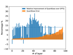
(a)	(b)

Figure 2: Comparison of the optimization performance of QuantEase and GPTQ over all layers. The horizontal dashed line shows the median improvement of QuantEase over GPTQ for each case. As can be seen, QuantEase results in lower optimization error compared to GPTQ for most layers (up to $30\%$ and on median 12%). Moreover, we see that the error in 3 bit quantization is larger than 4 bit quantization.

4 Outlier-Aware Quantization

4.1 Formulation

It has been observed that the activation might be more sensitive to some weights in a layer over others (Dettmers et al., 2023; Yao et al., 2022). For such sensitive weights, it might not be possible to find a suitable value on the quantization grid, leading to large quantization error. Moreover, some weights of a pre-trained network can be significantly larger or smaller than the rest—the quantization of LLMs can be affected by such weights (Wei et al., 2022b; Bondarenko et al., 2021; Kim et al., 2023). The existence of large/small weights increases the range of values that need to be quantized, which in turn increases quantization error. To this end, to better handle sensitive and large/small weights, which we collectively call outlier weights, we first introduce a modified version of the layerwise quantization problem (1). Our optimization formulation simultaneously identifies a collection of weights which are kept in full precision (aka the outliers weights) and quantizes the remaining weights.

Before presenting our outlier-aware quantization formulation, we introduce some notation. Let $\mathcal{S}\subseteq[q]\times[p]$ denote a set of outlier indices—the corresponding weights are left at full precision. For any $(i,j)\notin\mathcal{S}$, the $(i,j)$-th weight is quantized and is chosen from the quantization grid $\mathcal{Q}_{i}$ for the $i$-th channel. This is equivalent to substituting the set of weights for the layer $\boldsymbol{W}$ with $\hat{\boldsymbol{W}}+\hat{\boldsymbol{H}}$ where $\hat{\boldsymbol{W}}$ is quantized (like in Problem (1)) and $\hat{\boldsymbol{H}}$ is sparse, with only a few nonzeros. In particular, for any $(i,j)\notin\mathcal{S}$, we have $\hat{H}_{i,j}=0$ implying the $(i,j)$-th weight can only have a quantized component. As $\mathcal{S}$ has a small cardinality, $\hat{\boldsymbol{H}}$ is mostly zero. On the other hand, when $(i,j)\in\mathcal{S}$, we have $\hat{H}_{i,j}\neq 0$ and the corresponding weight is retained at full precision. In light of the above discussion, we present an outlier-aware version of Problem (1) given by:

$$\min_{\hat{\boldsymbol{W}},\hat{\boldsymbol{H}}}g(\hat{\boldsymbol{W}},\hat{\boldsymbol{H}}):=\|\boldsymbol{W}\boldsymbol{X}-(\hat{\boldsymbol{W}}+\hat{\boldsymbol{H}})\boldsymbol{X}\|_{F}^{2}~{}~{}\text{s.t.}~{}~{}\hat{W}_{i,j}\in\mathcal{Q}_{i}~{}(i,j)\in[q]\times[p],~{}~{}~{}~{}\|\hat{\boldsymbol{H}}\|_{0}\leq s$$ (14)

where $\|\cdot\|_{0}$ denotes the number of nonzero elements of a vector/matrix, and $s\ll p,q$ is the total budget on the number of outliers. The constraint $\|\hat{\boldsymbol{H}}\|_{0}\leq s$ ensures the total number of outliers remains within the specified limit.

4.2 SpQR

Before proceeding with our algorithm, we quickly review SpQR (Dettmers et al., 2023) which incorporates sensitivity-based quantization into GPTQ. Particularly, they seek to select few outliers that result in higher quantization error and keep them in full-precision. To this end, for each coordinate $(i,j)\in[q]\times[p]$ SpQR calculates the sensitivity to this coordinate as the optimization error resulting from quantizing this coordinate. Formally, they define sensitivity as

$$\omega_{ij}=\min_{\hat{\boldsymbol{W}}}\|\boldsymbol{W}\boldsymbol{X}-\hat{\boldsymbol{W}}\boldsymbol{X}\|_{F}^{2}~{}~{}~{}\text{s.t.}~{}~{}~{}\hat{W}_{i,j}=q_{i}(W_{i,j}).$$ (15)

We note that Problem (15) is in OBS form and therefore OBS is then used to calculate the sensitivity of coordinate $(i,j)$. Then, any coordinate that has high sensitivity, for example, $\omega_{i,j}>\tau$ where $\tau>0$ is a predetermined threshold, is considered to be an outlier. After selecting outliers, similar to GPTQ, SpQR cycles through columns $j=1,\cdots,p$ and updates each column based on OBS updates (see Section 2.2.1), keeping outlier weights in full-precision.

4.3 Optimizing Problem (14)

To obtain good solutions to Problem (14), we use a block coordinate descent method where we alternate between updating $\hat{\boldsymbol{W}}$ (with $\hat{\boldsymbol{H}}$ fixed) and then $\hat{\boldsymbol{H}}$ (with $\hat{\boldsymbol{W}}$ fixed). For a fixed $\hat{\boldsymbol{H}}$, Problem (14) has the same form as $f(\hat{\boldsymbol{W}})$ in (1) where $\boldsymbol{W}\boldsymbol{X}$ is substituted with $(\boldsymbol{W}-\hat{\boldsymbol{H}})\boldsymbol{X}$. Therefore, we can use QuantEase  as discussed in Section 3 to update $\hat{\boldsymbol{W}}$. Next, we discuss how to update $\hat{\boldsymbol{H}}$. For a fixed $\hat{\boldsymbol{W}}$, Problem (14) is a least squares problem with a cardinality constraint. We use proximal gradient method (aka iterative hard thresholding method) (Blumensath and Davies, 2009) where we make a series of updates of the form:

$$\hat{\boldsymbol{H}}^{+} \in\mathop{\mathrm{argmin}}_{\boldsymbol{K}}\tilde{g}(\boldsymbol{K})~{}~{}\text{s.t.}~{}~{}\|\boldsymbol{K}\|_{0}\leq s=P_{s}(\hat{\boldsymbol{H}}-\eta\nabla_{\boldsymbol{H}}g(\hat{\boldsymbol{W}},\hat{\boldsymbol{H}}))$$ (16)

where $P_{s}(\boldsymbol{A})$ sets all coordinates of $\boldsymbol{A}$ to zero except the $s$-largest in absolute value,

$$\tilde{g}(\boldsymbol{K})=\frac{L}{2}\left\|\boldsymbol{K}-\left(\hat{\boldsymbol{H}}-\frac{1}{L}\nabla_{\hat{\boldsymbol{H}}}g(\hat{\boldsymbol{W}},\hat{\boldsymbol{H}})\right)\right\|_{F}^{2},$$ (17)

$L=1/\eta=2\lambda_{\max}(\boldsymbol{X}\boldsymbol{X}^{T})$ and $\lambda_{\max}(\boldsymbol{A})$ is the largest eigenvalue of the matrix $\boldsymbol{A}$. Lemma 3 below establishes updates in (16) form a descent method if the initial $\hat{\boldsymbol{H}}$ is sparse, $\|\hat{\boldsymbol{H}}\|_{0}\leq s$.

Lemma 3.

For any $\hat{\boldsymbol{W}}$ and any $\hat{\boldsymbol{H}}$ such that $\|\hat{\boldsymbol{H}}\|_{0}\leq s$, we have

$$g(\hat{\boldsymbol{W}},\hat{\boldsymbol{H}}^{+})\leq g(\hat{\boldsymbol{W}},\hat{\boldsymbol{H}}).$$

We note that when calculating $\mathcal{Q}_{i}$’s for Problem (14), we remove the top $s$ largest coordinates of $\boldsymbol{W}$ (in absolute value) from the quantization pool, as the effect of those weights can be captured by $\hat{\boldsymbol{H}}$ and we do not need to quantize them. This allows to reduce the range that each $\mathcal{Q}_{i}$ needs to quantize, leading to lower error. Therefore, simultaneously, we preserve sensitive weights and reduce the quantization range by using outlier-aware QuantEase.

The details of the update discussed here are presented in Algorithm 3. In terms of initialization, similar to basic QuantEase, we set $\hat{\boldsymbol{H}},\hat{\boldsymbol{W}}$ such that $\hat{\boldsymbol{H}}+\hat{\boldsymbol{W}}=\boldsymbol{W}$. Particularly, we use the $s$-largest coordinates of $\boldsymbol{W}$ (in absolute value) to initialize $\hat{\boldsymbol{H}}$: $\hat{\boldsymbol{H}}=P_{s}(\boldsymbol{W}),\hat{\boldsymbol{W}}=\boldsymbol{W}-\hat{\boldsymbol{H}}$. Note that this leads to an infeasible initialization of $\hat{\boldsymbol{W}}$ similar to basic QuantEase. However, as discussed in Section 3.1, after one iteration of QuantEase the solution becomes feasible and the descent property of Algorithm 3 holds.

We also note that as seen from Algorithm 3, in addition to storing $\hat{\boldsymbol{H}}$, we need to store $\hat{\boldsymbol{H}}\boldsymbol{\Sigma}$, showing the memory footprint remains $p^{2}+\mathcal{O}(pq)$, like basic QuantEase. In terms of computational complexity, in addition to basic QuantEase, the outlier-aware version requires calculating the largest eigenvalue of $\boldsymbol{X}\boldsymbol{X}^{T}$, which can be done by iterative power method in $\mathcal{O}(p^{2})$ only using matrix/vector multiplication. Additionally, calculating $\hat{\boldsymbol{H}}\boldsymbol{\Sigma}$ requires $\mathcal{O}(p^{2}q)$ in each iteration, and finding the largest $s$ coordinates of $\hat{\boldsymbol{H}}$ can be done with average complexity of $\mathcal{O}(pq\log pq)$. Therefore, the overall complexity is $\mathcal{O}(pqn+Kp^{2}q+Kpq\log pq)$ for $K$ iterations.

Finally, we note that unlike SpQR which fixes the location of outliers after selecting them, our method is able to add new outlier coordinates or remove them as the optimization progresses. This is because the location of nonzeros of $\hat{\boldsymbol{H}}$ (i.e. outliers) gets updated, in addition to their values.

Structured Outliers: Problem (14) does not have any constraints on the structure of the outliers. Serving a model with unstructured outliers may lead to increased serving latency because of added complexity to the GPU kernel implementation.

A simple change to make the algorithm outlier aware is to constrain the selection of the outliers to be entire columns when performing the update in Equation (16). Instead of choosing the $s$-largest absolute values of $\boldsymbol{A}$ with $P_{s}$, we can choose columns with the $\lfloor\frac{s}{q}\rfloor$-largest $l2$ norm values, treating them as the most influential columns to keep as the outliers with full (or higher) precision. In practice, we can select different versions of the outlier-aware algorithm depending on the serving dequantization kernel implementation to balance the trade-off between serving efficiency and model accuracy. This exploration is beyond the scope of this paper. Empirical comparisons between various outlier-aware algorithms can be found in Section 5.4

5 Experiments

In this section, we conduct several numerical experiments to demonstrate the effectiveness of QuantEase. A PyTorch-based implementation of QuantEase will be released on GitHub soon.

Experimental Setup. For uniform quantization, we compare QuantEase to RTN (Yao et al., 2022; Dettmers et al., 2022), GPTQ (Frantar et al., 2023) and AWQ (Lin et al., 2023). For methods related to outlier detection, we compare with SpQR (Dettmers et al., 2023). We do not consider SqueezeLLM (Kim et al., 2023) as it mainly focuses on non-uniform quantization (whereas we focus on uniform quantization). Moreover, to the best of our knowledge, the quantization code for SqueezeLLM has not been made publicly available. In our experiments, we do not use grouping for any method as our focus on understanding the optimization performance of various methods. Moreover, as discussed by Kim et al. (2023); Yao et al. (2023), grouping can lead to additional inference-time overhead, reducing the desirability of such tricks in practice.

In terms of models and data, we consider several models from the OPT (Zhang et al., 2022), BLOOM (Laurençon et al., 2022), and Falcon (Penedo et al., 2023) families of LLMs. Note that we do not run AWQ on the BLOOM and Falcon models due to known architectural issues . For the calibration (training) data, we randomly choose 128 sequences of length 2048 from the C4 dataset (Raffel et al., 2020). For validation data, following Frantar et al. (2023), we use datasets WikiText2 (Merity et al., 2016) and PTB (Marcus et al., 1994) in our experiments. In particular, after quantizing the model using the data from C4, we evaluate the model performance on PTB and WikiText2. Our experiments were conducted on a single NVIDIA A100 GPU with 80GB of memory. Notably, for the OPT-66b model,  QuantEase works on a single NVIDIA V100 GPU whereas GPTQ (due to Cholesky factorization) and AWQ (due to batched calculations) ran out of memory. This further highlights the memory efficacy of QuantEase.

Additional Experiments: Appendix A contains additional numerical results related to runtime and text generation.

5.1 Effect of Number of Iterations

We first study the effect of the number of iterations of QuantEase on model performance. To this end, we consider OPT-350m in 3/4 bits and run quantization for different numbers of iterations, ranging from 10 to 30. The perplexity on WikiText2 is shown in Figure 3 for this case. The results show that increasing the number of iterations generally lowers perplexity as QuantEase reduces the error, although the improvement in perplexity for 4-bit quantization is small. Based on these results, 25 iterations seem to strike a good balance between accuracy and runtime, which we use in the rest of our experiments.

Effect of number of iterations

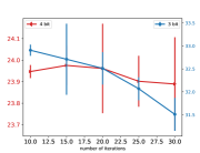
Figure 3: Effect of varying the number of iterations of QuantEase on perplexity in Section 5.1.

5.2 Language Generation Benchmarks

Next, we study the effect of quantization on language generation tasks. Perplexity results for the WikiText2 data and OPT/BLOOM/Falcon families are shown in Tables 1, 2, and 3 respectively. Perplexity results for the PTB data can be found in Tables A.1, A.2, and A.3 in the Appendix. QuantEase achieves lower perplexity in all cases for 3-bit quantization. In the 4-bit regime, QuantEase  almost always either improves upon baselines or achieves similar performance. Since perplexity is a stringent measure of model quality, these results demonstrate that QuantEase results in better quantization compared to methods like GPTQ and AWQ.

		350m	1.3b	2.7b	6.7b	13b	66b
full		22.00	$14.62$	12.47	10.86	10.13	9.34
3 bits	RTN	64.56	1.33e4	1.56e4	6.00e3	3.36e3	$6.12e3$
	AWQ	${32.38}_{0.11}$	$53.63_{0.45}$	$201_{6}$	$19.00_{0.12}$	$13.90_{0.02}$	$17.94_{0.18}$
	GPTQ	$33.60_{0.34}$	$21.51_{0.13}$	$17.02_{0.17}$	$15.16_{0.01}$	$\textbf{11.90}_{0.06}$	$14.13_{0.43}$
	QuantEase	$\textbf{31.52}_{0.36}$	$\textbf{21.30}_{0.23}$	$\textbf{16.75}_{0.24}$	$\textbf{12.95}_{0.04}$	$12.41_{0.02}$	$\textbf{13.08}_{0.38}$
4 bits	RTN	25.94	48.19	16.92	12.10	11.32	110.52
	AWQ	$24.05_{0.03}$	$15.67_{0.04}$	$13.16_{0.01}$	$11.30_{0.01}$	$10.36_{0.01}$	$9.58_{0.01}$
	GPTQ	$24.29_{0.11}$	$15.44_{0.03}$	$\textbf{12.80}_{0.04}$	$11.46_{0.04}$	$10.34_{0.01}$	$9.58_{0.05}$
	QuantEase	$\textbf{23.91}_{0.05}$	$\textbf{15.28}_{0.04}$	$13.05_{0.01}$	$\textbf{11.21}_{0.01}$	$\textbf{10.32}_{0.01}$	$\textbf{9.47}_{0.02}$

Table 1: OPT family perplexity for WikiText2 quantized on C4. QuantEase achieves lower perplexity in the majority of settings.

		560m	1b1	1b7	3b	7b1
full		22.41	17.68	15.39	13.48	11.37
3 bits	RTN	56.99	50.07	63.50	39.29	17.37
	GPTQ	$32.36_{0.07}$	$25.18_{0.06}$	$21.43_{0.07}$	$17.50_{0.04}$	$13.73_{0.03}$
	QuantEase	$\textbf{31.52}_{0.10}$	$\textbf{23.91}_{0.02}$	$\textbf{20.03}_{0.05}$	$\textbf{17.21}_{0.04}$	$\textbf{13.43}_{0.04}$
4 bits	RTN	25.89	19.98	16.97	14.75	12.10
	GPTQ	$24.02_{0.03}$	$\textbf{18.90}_{0.02}$	$16.41_{0.02}$	$\textbf{14.10}_{0.01}$	$11.74_{0.01}$
	QuantEase	$\textbf{23.97}_{0.03}$	$\textbf{18.90}_{0.01}$	$\textbf{16.11}_{0.03}$	$14.18_{0.01}$	$\textbf{11.69}_{0.01}$

Table 2: BLOOM family perplexity for WikiText2 quantized on C4. QuantEase achieves lower perplexity in the majority of settings.

		7b	40b	180b
full		6.59	5.23	3.30
3 bits	RTN	5.67e2	3.89e7	1.55e4
	GPTQ	$9.62_{0.13}$	N/A	N/A
	QuantEase	$\mathbf{8.83}_{0.07}$	$\mathbf{6.20}_{0.07}$	$\mathbf{5.19}_{0.10}$
4 bits	RTN	9.96	5.67	36.63
	GPTQ	$\mathbf{6.90}_{0.01}$	$\mathbf{5.35}$*	N/A
	QuantEase	$6.92_{0.01}$	$5.36_{0.02}$	$\mathbf{3.72}_{0.01}$

• Only one seed succeeds among all trials while the rest have numerical issues, thus no standard deviation is reported here.

Table 3: Falcon family perplexity for WikiText2 quantized on C4. QuantEase achieves lower perplexity in the majority of settings. GPTQ has numerical issue with most of the seeds we explored when computing Cholesky factorization when quantizing the Falcon-40b and 180b models with the default setup. We run a single iteration for QuantEase on Falcon-180b to prevent overfitting.

5.3 LAMBADA Zero-Shot Benchmark

Following (Frantar et al., 2023), we compare the performance of our method with baselines over a zero-shot task, namely LAMBADA (Paperno et al., 2016). The results for this task are shown in Figure 4 for the OPT and BLOOM families. For 3-bit quantization, QuantEase outperforms GPTQ and AWQ, often by a large margin. In the 4-bit regime, the performance of all methods is similar, although QuantEase is shown to be overall the most performant.

Figure 4: Zero-Shot accuracy on the LAMBADA (Paperno et al., 2016) benchmark for 3-bit and 4-bit quantization. See Section 5.3 for more details on experimental setup.

5.4 Outliers-Aware Performance

Next, we study the performance of the outlier-aware version of QuantEase. To this end, we consider 3-bit quantization and two sparsity levels of $0.5\%$ and $1\%$ (for example, $s=0.005pq$ or $s=0.01pq$). Roughly speaking, a $0.5\%$ outlier budget would lead to an additional 0.15 bits overhead (i.e. 3.15 bits on average), while the $1\%$ version would lead to an additional overhead of 0.3 bits (i.e. 3.3 bits on average). We compare our method with SpQR, with the threshold tuned to have at least $1\%$ outliers on average. The rest of the experimental setup is shared from previous experiments. The perplexity results (on WikiText2) for this comparison are reported in Table 4 for the OPT family and in Table A.4 for the BLOOM family. Table A.6 contains results for the Falcon family. As is evident from the results, the QuantEase $0.5\%$ outlier version is able to significantly outperform SpQR in all cases, and the $1\%$ method does even better. This shows that outlier-aware QuantEase makes near-3 bit quantization possible without the need for any grouping.

5.4.1 Extreme Quantization

Next, we study extreme quantization of models to the 2-bit regime. Particularly, we consider the base number of bits of 2 and $2\%$ outliers, resulting in roughly 2.6 bits on average. The results for this experiment for OPT are shown in Table 5 and for BLOOM in Table A.5. QuantEase significantly outperforms SpQR and is able to maintain acceptable accuracy in the sub-3-bit quantization regime.

We observed empirically that in the absence of grouping and outlier detection, if we were to do 2-bit quantization, then the resulting solutions lead to a significant loss of accuracy. This finding also appears to be consistent with our exploration of other methods’ publicly available code, such as GPTQ and AWQ.

		350m	1.3b	2.7b	6.7b	13b
full		22.00	$14.62$	12.47	10.86	10.13
3 bits	QuantEase	${31.52}_{0.12}$	${21.30}_{0.23}$	${16.75}_{0.24}$	${12.95}_{0.04}$	$12.41_{0.02}$
Outlier (3 bits)	SpQR $1\%$	$31.67_{0.43}$	$18.17_{0.16}$	$14.50_{0.07}$	$11.95_{0.02}$	$10.96_{0.01}$
	QuantEase $0.5\%$	${27.52}_{0.05}$	${16.68}_{0.14}$	${13.72}_{0.04}$	$11.49_{0.02}$	$10.70_{0.01}$
	QuantEase $1\%$	${26.48}_{0.12}$	${16.25}_{0.05}$	$13.70_{0.10}$	$11.48_{0.03}$	$10.37_{0.01}$
	QuantEase structured   $0.5\%$	${31.09}_{0.86}$	${18.86}_{0.36}$	${15.80}_{0.37}$	${12.15}_{0.06}$	${12.18}_{0.04}$
	QuantEase structured   $1\%$	${30.21}_{0.16}$	${18.51}_{0.27}$	${15.65}_{0.04}$	${12.26}_{0.01}$	${12.07}_{0.13}$
4 bits	QuantEase	${23.91}_{0.05}$	${15.28}_{0.04}$	$13.05_{0.01}$	${11.21}_{0.01}$	$10.32_{0.01}$

Table 4: OPT family perplexity for WikiText2 quantized on C4. Outlier aware quantization is done with 3 bits.

		350m	1.3b	2.7b	6.7b	13b
full		22.00	$14.62$	12.47	10.86	10.13
Outlier (2 bits)	SpQR $2\%$	$323_{7}$	$155_{3}$	$70.5_{2.7}$	$34.0_{1.2}$	$22.3_{0.2}$
	QuantEase $2\%$	$\textbf{158}_{4}$	$\textbf{36.4}_{0.8}$	$\textbf{24.2}_{0.1}$	$\textbf{19.0}_{0.2}$	$\textbf{19.3}_{0.2}$

Table 5: OPT family perplexity for WikiText2 quantized on C4. Outlier aware quantization is done with 2 bits.

6 Discussion

We study PTQ of LLMs and proposed a new layerwise PTQ framework, QuantEase. QuantEase is based on cyclic CD with simple updates for each coordinates. We also introduce an outlier aware version of QuantEase.

Our numerical experiments show that our method outperforms the state-of-the-art methods such as GPTQ and AWQ for 3/4 bit uniform quantization. Our outlier aware QuantEase outperforms SpQR when quantizing to near- or sub-3 bit regimes.

In this work, we did not consider grouping. However, we note that grouping can be easily incorporated in QuantEase, as we only use standard quantizers. Investigating the performance of QuantEase with grouping is left for a future study. Moreover, we note that QuantEase can be paired with AWQ. As Lin et al. (2023) note, incorporating AWQ into GPTQ can lead to improved numerical results, and as we have shown, QuantEase usually outperforms GPTQ. Therefore, we would expect AWQ+QuantEase would lead to even further improvements.

Appendix A Numerical Results

		350m	1.3b	2.7b	6.7b	13b	66b
full		26.08	16.96	15.11	13.09	12.34	11.36
3 bits	RTN	81.09	1.16e4	9.39e3	4.39e3	2.47e3	3.65e3
	AWQ	$40.20_{0.07}$	$98.12_{2.26}$	$188_{4}$	$26.07_{0.14}$	$19.96_{0.05}$	$27.45_{0.29}$
	GPTQ	$39.28_{0.04}$	$26.36_{0.14}$	$19.98_{0.13}$	$18.86_{0.02}$	$\textbf{13.88}_{0.03}$	$15.10_{0.25}$
	QuantEase	$\textbf{37.70}_{0.15}$	$\textbf{25.24}_{0.27}$	$\textbf{19.90}_{0.05}$	$\textbf{15.78}_{0.06}$	$\textbf{13.89}_{0.02}$	$\textbf{12.93}_{0.19}$
4 bits	RTN	31.12	34.15	22.11	16.09	15.39	274.56
	AWQ	$29.30_{0.02}$	$18.82_{0.08}$	$16.40_{0.01}$	$13.86_{0.01}$	$12.77_{0.01}$	$11.68_{0.01}$
	GPTQ	$28.84_{0.09}$	$18.44_{0.01}$	$\textbf{15.87}_{0.01}$	$13.78_{0.05}$	$12.59_{0.01}$	$11.60_{0.01}$
	QuantEase	$\textbf{28.49}_{0.10}$	$\textbf{18.23}_{0.04}$	$15.95_{0.01}$	$\textbf{13.56}_{0.03}$	$\textbf{12.50}_{0.01}$	$\textbf{11.55}_{0.01}$

Table A.1: OPT family perplexity for PTB quantized on C4

		560m	1b1	1b7	3b	7b1
full		41.23	46.96	27.92	23.12	19.40
3 bits	RTN	117.17	151.76	115.10	59.87	32.03
	GPTQ	$64.63_{0.65}$	$72.57_{0.70}$	$42.48_{0.04}$	$31.36_{0.1}$	$24.34_{0.05}$
	QuantEase	$\textbf{59.37}_{0.40}$	$\textbf{69.61}_{0.51}$	$\textbf{38.92}_{0.30}$	$\textbf{30.59}_{0.2}$	$\textbf{23.73}_{0.06}$
4 bits	RTN	48.56	54.51	31.20	25.39	20.92
	GPTQ	$44.35_{0.09}$	$51.64_{0.07}$	$30.10_{0.06}$	$24.33_{0.01}$	$20.21_{0.04}$
	QuantEase	$\textbf{43.90}_{0.04}$	$\textbf{51.60}_{0.34}$	$\textbf{29.50}_{0.17}$	$\textbf{24.22}_{0.03}$	$\textbf{20.11}_{0.01}$

Table A.2: BLOOM family perplexity for PTB quantized on C4

		7b	40b	180b
full		9.90	7.83	6.65
3 bits	RTN	5.85e2	2.63e6	1.42e4
	GPTQ	$13.64_{0.13}$	N/A	N/A
	QuantEase	$\mathbf{13.28}_{0.04}$	$\mathbf{8.94}_{0.03}$	$\mathbf{7.76}_{0.04}$
4 bits	RTN	12.84	8.61	60.44
	GPTQ	$10.40_{0.03}$	$8.01$*	N/A
	QuantEase	$\mathbf{10.39}_{0.02}$	$\mathbf{8.01}_{0.01}$	$\mathbf{6.90}_{0.02}$

• Only one seed succeeds among all trials while the rest have numerical issues, thus no standard deviation is reported here.

Table A.3: Falcon family perplexity for PTB quantized on C4. GPTQ has numerical issue when computing Cholesky factorization when quantizing the falcon-40b and 180b with default setup described in the original paper on most seeds. We run single iter for QuantEase on Falcon-180b to prevent overfitting issue.

A.1 Additional Text Generation Benchmarks

First, we present the results for uniform quantization evaluated on PTB dataset (the setup from Section 5.2). These results can be found in Tables A.1, A.2, and A.3. Additional outlier aware quantization results are presented in Tables A.4 and A.5 for BLOOM family and Tables A.6 for Falcon family from Section 5.4.

		560m	1b1	1b7	3b	7b1
full		22.41	17.68	15.39	13.48	11.37
3 bits	QuantEase	${31.52}_{0.10}$	${23.91}_{0.02}$	${20.03}_{0.05}$	${17.21}_{0.04}$	${13.43}_{0.04}$
Outlier (3 bits)	SpQR $1\%$	$29.02_{0.05}$	$22.51_{0.11}$	$19.16_{0.05}$	$15.95_{0.06}$	$12.88_{0.01}$
	QuantEase $0.5\%$	${26.82}_{0.07}$	${20.26}_{0.03}$	${17.41}_{0.02}$	$14.93_{0.01}$	$12.19_{0.01}$
	QuantEase $1\%$	$25.80_{0.09}$	${19.60}_{0.02}$	${17.06}_{0.02}$	$14.65_{0.02}$	$12.03_{0.01}$
	QuantEase structured   $0.5\%$	${29.42}_{0.39}$	${22.56}_{0.06}$	${18.97}_{0.06}$	${16.23}_{0.06}$	${12.95}_{0.06}$
	QuantEase structured   $1\%$	${29.00}_{0.24}$	${22.49}_{0.12}$	${18.89}_{0.05}$	${15.99}_{0.06}$	${12.97}_{0.04}$
4 bits	QuantEase	${23.97}_{0.03}$	${18.90}_{0.01}$	${16.11}_{0.03}$	$14.18_{0.01}$	${11.69}_{0.01}$

Table A.4: BLOOM family perplexity for WikiText2 quantized on C4. Outlier aware quantization is done with 3 bits.

		560m	1b1	1b7	3b	7b1
full		22.41	17.68	15.39	13.48	11.37
Outlier (2 bits)	SpQR $2\%$	$228_{10}$	$126_{5}$	$127_{4}$	$59.7_{2.2}$	$32.5_{0.4}$
	QuantEase $2\%$	$\textbf{66.1}_{1.3}$	$\textbf{39.3}_{0.3}$	$\textbf{31.4}_{0.1}$	$\textbf{22.1}_{0.1}$	$\textbf{15.8}_{0.03}$

Table A.5: BLOOM family perplexity for WikiText2 quantized on C4. Outlier aware quantization is done with 2 bits.

		7b	40b	180b
full		6.59	5.23	3.30
3 bits	QuantEase	$8.83_{0.07}$	$6.20_{0.07}$	$5.19_{0.10}$
Outlier (3 bits)	SpQR $1\%$	$8.38_{0.08}$	N/A	N/A
	QuantEase  $0.5\%$	$7.29_{0.03}$	$5.54_{0.01}$	$3.91_{0.01}$
	QuantEase  $1\%$	$7.14_{0.01}$	$5.51_{0.01}$	$3.79_{0.01}$
	QuantEase structured   $0.5\%$	$8.66_{0.06}$	$6.02_{0.02}$	$4.88_{0.06}$
	QuantEase structured   $1\%$	$8.56_{0.01}$	$5.99_{0.03}$	$4.81_{0.05}$
4 bits	QuantEase	$6.92_{0.01}$	$5.36_{0.02}$	${3.72}_{0.01}$

Table A.6: Falcon family perplexity for WikiText2 quantized on C4. Outlier aware quantization is done with 3 bits. SpQR has numerical issue when computing Cholesky factorization when quantizing the falcon-40b and 180b with default setup. We run single iter for QuantEase on Falcon-180b to prevent overfitting issue.

		7b	40b	180b
full		6.59	5.23	3.30
Outlier (2 bits)	SpQR $2\%$	${24.91}_{0.76}$	${8.83}_{0.07}$	N/A
	QuantEase $2\%$	$\mathbf{11.37}_{0.22}$	$\mathbf{6.73}_{0.06}$	$\mathbf{5.63}_{0.23}$

Table A.7: Falcon family perplexity for WikiText2 quantized on C4. Outlier aware quantization is done with 2 bits.

A.2 Generative Examples

In this section, we present a few generative examples. We have used OPT-13b model quantized to 4 bits in all examples here.

A.2.1 Example 1

• Prompt: Every time data scientist Kim ran her new algorithm, it kept outputting the same
unexpected result: a recipe for

• FP16: Every time data scientist Kim ran her new algorithm, it kept outputting the same
unexpected result: a recipe for a new kind of chocolate cake. The algorithm was designed
to predict the likelihood that a person would be a repeat customer of a particular
restaurant. But it kept coming up with a recipe for a chocolate cake.
"I was like, ’What’?" Kim said. "I was like, ’This is not what I asked for’".

• GPTQ: Every time data scientist Kim ran her new algorithm, it kept outputting the same
unexpected result: a recipe for a new kind of chocolate cake. Kim, who asked to be
identified by her first name only, was working on a project to predict the likelihood
of a person being a criminal. She was using a machine learning algorithm to analyze data
from the FBI’s National Crime Information Center, which contains information on more
than 10 million criminal records.

• QuantEase: Every time data scientist Kim ran her new algorithm, it kept outputting the same
unexpected result: a recipe for a new drug. The algorithm was designed to predict
the likelihood that a drug would be approved by the US Food and Drug Administration (FDA).
But it kept coming up with a recipe for a new drug that was never approved.
"It was a bit of a shock," says Kim, a data scientist at the University of California,
San Francisco.

In this case, although GPTQ’s response is initially similar to the FP16 response (both outputting chocolate cake), as the response continues, GPTQ and FP16 diverge. On the other hand, QuantEase produces a response that is overall coherent and logical. This is while GPTQ’s response relates food to crime.

A.2.2 Example 2

• Prompt: In a parallel universe where cats are the rulers of Earth, our feline king
was pondering his first decree

• FP16: In a parallel universe where cats are the rulers of Earth, our feline king
was pondering his first decree. "I decree that all cats shall be given the right to vote,"
he said. "And I decree that all cats shall be given the right to vote,"
said the cat next to him.

• GPTQ: In a parallel universe where cats are the rulers of Earth, our feline king
was pondering his first decree."I decree that all cats shall be allowed to roam free,"
he said. "And I decree that all cats shall be allowed to eat as much as they want,"
said a second cat. "And I decree that all cats shall be allowed to sleep
as much as they want," said a third cat.

• QuantEase: In a parallel universe where cats are the rulers of Earth, our feline king
was pondering his first decree. "I decree that all cats shall be allowed to sleep
on the bed," he said. "But only if they are on their backs," said his advisor.
"But only if they are on their backs," said the king.

In this case, both GPTQ and QuantEase diverge from the FP16 model, although the response from both seems to be coherent. However, we note that QuantEase is able to mention the “advisor” and “king” keeping the context relevant, while GPTQ refers to “second cat” and so on.

A.2.3 Example 3

• Prompt: Data scientist Grace was working late one night when she discovered a glitch
in the matrix of her data. It spelled out

• FP16: Data scientist Grace was working late one night when she discovered a glitch
in the matrix of her data. It spelled out the word "HELP" in the form of a series of
numbers. She was able to use the glitch to access a hidden database that contained the
names and addresses of all the people who had ever used the service.

• GPTQ: Data scientist Grace was working late one night when she discovered a glitch
in the matrix of her data. It spelled out the word "HELP" in the form of a series of
numbers. She was so excited that she called her friend, a programmer, and told him
about it. "I’m not sure what you’re talking about," he said.
"I’ve never seen that before." "Well,

• QuantEase: Data scientist Grace was working late one night when she discovered a glitch
in the matrix of her data. It spelled out the word "HELP" in the form of a series of
numbers. She was able to use the glitch to access a hidden database that contained
the names of all the people who had ever been in the database. She was able
to access the names of all the people who had ever been in the database.

In this case, QuantEase seems to be closer to the FP16 response, although QuantEase repeats itself at the end of the sentence, showing QuantEase might lose the attention in this case.

A.2.4 Example 4

• Prompt: Last Tuesday, just as the sun was setting, my neighbor’s dog, Rover, started
to speak to me in perfect French. He said

• FP16: Last Tuesday, just as the sun was setting, my neighbor’s dog, Rover, started
to speak to me in perfect French. He said, "I’m sorry, I don’ speak English." I was shocked.
I’ve lived in this neighborhood for over a year and Rover has never spoken to me before.
I’ve never seen him before. I’ve never heard him before.

• GPTQ: Last Tuesday, just as the sun was setting, my neighbor’s dog, Rover, started
to speak to me in perfect French. He said, "I’m Rover. I’m a dog. I’m a dog."
I was stunned. I was speechless. I was in awe. I’ve been a dog lover all my life.
I’ve always had dogs. I’ve always loved dogs. I’ve always wanted to be a

• QuantEase: Last Tuesday, just as the sun was setting, my neighbor’s dog, Rover, started
to speak to me in perfect French. He said, "I’m sorry, I’m so sorry." I was in
the middle of a conversation with my friend, and I stopped to listen to Rover. He was
standing in the middle of the street, looking up at the sky. "I’m sorry, I’m so
sorry," he said again.

In this case, none of the models appear to follow FP16 response.

A.3 Runtime

In this section, we report the runtime of our QuantEase method. The numbers reported are for 3-bit quantization experiments from Tables 1,  2, and 3 for OPT, BLOOM, and Falcon families, respectively. The runtime for different models are reported in Tables A.8, A.9, and A.10. We see that the runtime ranges from 10s of minutes for sub-billion models, up to around a day for 13b model. This shows that overall, QuantEase is computationally feasible, specially for models with 10b or fewer parameters.

	350m	1.3b	2.7b	6.7b	13b	66b
QuantEase	25.8m	52.6m	1.4h	2.4h	3.8h	13.8h

Table A.8: QuantEase runtime for OPT family

	560m	1b1	1b7	3b	7b1
QuantEase	19.5m	29.6m	40.6m	1.1h	1.9h

Table A.9: QuantEase runtime for BLOOM family

	7b	40b	180b
QuantEase	2.3h	13.0h	2.9h (1 iter)

Table A.10: QuantEase runtime for Falcon family. We run 30 iterations on Falcon 7b/40b and 1 iter on Falcon-180b to prevent overfitting.

Appendix B Proof of Main Results

B.1 Proof of Lemma 1

Write

$$f(\hat{\boldsymbol{W}}) =\|\boldsymbol{W}\boldsymbol{X}-\hat{\boldsymbol{W}}\boldsymbol{X}\|_{F}^{2}$$

$$=\left\|\sum_{j=1}^{p}\hat{\boldsymbol{W}}_{:,j}\boldsymbol{X}_{j,:}-\boldsymbol{W}\boldsymbol{X}\right\|_{F}^{2}$$

$$\stackrel{{\scriptstyle(a)}}{{=}}\sum_{j,k=1}^{p}\mathsf{Tr}(\boldsymbol{X}_{j,:}^{T}\hat{\boldsymbol{W}}_{:,j}^{T}\hat{\boldsymbol{W}}_{:,k}\boldsymbol{X}_{k,:})+\mathsf{Tr}(\boldsymbol{X}^{T}\boldsymbol{W}^{T}\boldsymbol{W}\boldsymbol{X})-2\sum_{j=1}^{p}\mathsf{Tr}(\boldsymbol{X}_{j,:}^{T}\hat{\boldsymbol{W}}_{:,j}^{T}\boldsymbol{W}\boldsymbol{X})$$

$$=\underbrace{\sum_{j,k=1}^{p}(\boldsymbol{X}_{k,:}\boldsymbol{X}_{j,:}^{T}\hat{\boldsymbol{W}}_{:,j}^{T}\hat{\boldsymbol{W}}_{:,k})}_{(A)}+\mathsf{Tr}(\boldsymbol{X}\boldsymbol{X}^{T}\boldsymbol{W}^{T}\boldsymbol{W})-\underbrace{2\sum_{j=1}^{p}\mathsf{Tr}(\boldsymbol{W}\boldsymbol{X}\boldsymbol{X}_{j,:}^{T}\hat{\boldsymbol{W}}_{:,j}^{T})}_{(B)}$$ (B.1)

where $(a)$ is by $\|\boldsymbol{A}\|_{F}^{2}=\mathsf{Tr}(\boldsymbol{A}^{T}\boldsymbol{A})$ and $(b)$ is by $\mathsf{Tr}(\boldsymbol{A}\boldsymbol{B})=\mathsf{Tr}(\boldsymbol{B}\boldsymbol{A})$. Next, let us only consider terms in (B.1) that depend on $\boldsymbol{W}_{:,j_{0}}$ for a given $j_{0}$. Letting $\boldsymbol{\Sigma}=\boldsymbol{X}\boldsymbol{X}^{T}$, such terms can be written as

$$\overbrace{(\boldsymbol{X}_{j_{0},:}\boldsymbol{X}_{j_{0},:}^{T}\hat{\boldsymbol{W}}_{:,j_{0}}^{T}\hat{\boldsymbol{W}}_{:,j_{0}})}^{\text{from}~{}(A),~{}j=k=j_{0}}+\overbrace{2\sum_{k\neq j_{0}}(\boldsymbol{X}_{j_{0},:}\boldsymbol{X}_{k,:}^{T}\hat{\boldsymbol{W}}_{:,k}^{T}\hat{\boldsymbol{W}}_{:,j_{0}})}^{\text{from}~{}(A),~{}~{}j~{}\text{or}~{}k~{}=~{}j_{0}}-\overbrace{2\mathsf{Tr}(\boldsymbol{W}\boldsymbol{X}\boldsymbol{X}_{j_{0},:}^{T}\hat{\boldsymbol{W}}_{:,j_{0}}^{T})}^{\text{from}~{}(B),~{}j=j_{0}}$$

$$= \sum_{i=1}^{q}\Sigma_{j_{0},j_{0}}\hat{W}_{i,j_{0}}^{2}+2\sum_{i=1}^{q}\sum_{k\neq j_{0}}\Sigma_{j_{0},k}\hat{W}_{i,j_{0}}\hat{W}_{i,k}-2\sum_{i=1}^{q}(\boldsymbol{W}\boldsymbol{\Sigma})_{i,j_{0}}\hat{W}_{i,j_{0}}$$

$$= \sum_{i=1}^{q}\left\{\Sigma_{j_{0},j_{0}}\hat{W}_{i,j_{0}}^{2}+2\sum_{k\neq j_{0}}\Sigma_{j_{0},k}\hat{W}_{i,j_{0}}\hat{W}_{i,k}-2(\boldsymbol{W}\boldsymbol{\Sigma})_{i,j_{0}}\hat{W}_{i,j_{0}}\right\}.$$ (B.2)

Therefore, to find the optimal value of $\hat{W}_{i,j}^{+}$ in (9) for $(i,j_{0})$ we need to solve problems of the form

$$\min_{u\in\mathcal{Q}_{i}}\Sigma_{j_{0},j_{0}}u^{2}+2\sum_{k\neq j_{0}}\Sigma_{j_{0},k}\hat{W}_{i,k}u-2(\boldsymbol{W}\boldsymbol{\Sigma})_{i,j_{0}}u.$$ (B.3)

Claim: If $a>0$, then

$$\min_{u\in\mathcal{Q}_{i}}au^{2}+bu=q_{i}(-b/2a).$$

Proof of Claim: Write

$$au^{2}+bu=a(u+(b/2a))^{2}-b^{2}/(4a)$$

therefore,

$$\mathop{\mathrm{argmin}}_{u\in\mathcal{Q}_{i}}au^{2}+bu =\mathop{\mathrm{argmin}}_{u\in\mathcal{Q}_{i}}(u+b/(2a))^{2}$$

$$=\mathop{\mathrm{argmin}}_{u\in\mathcal{Q}_{i}}(u+b/(2a))^{2}$$

$$=\mathop{\mathrm{argmin}}_{y\in\mathcal{Q}_{i}+b/(2a)}y^{2}-b/(2a)$$

$$=\tilde{q}_{i}(0)-b/(2a)$$

$$=q(-b/(2a))$$ (B.4)

where $\tilde{q}_{i}$ is the quantization function for the quantization grid $\mathcal{Q}_{i}+b/(2a)=\{a+b/(2a):a\in\mathcal{Q}_{i}\}$. This completes the proof of the claim and the lemma.

B.2 Proof of Lemma 2

The proof is a result of the observations that (a) the modified algorithm generates a sequence of $\hat{\boldsymbol{W}}$ iterates with decreasing $f$ values (after obtaining the first feasible solution, possibly after the first iteration) and (b) there are only a finite number of choices for $\hat{\boldsymbol{W}}$ on the quantization grid.

B.3 Proof of Lemma 3

First, note that mapping $\hat{\boldsymbol{H}}\mapsto\nabla_{\boldsymbol{H}}g(\hat{\boldsymbol{W}},\hat{\boldsymbol{H}})$ is $L$-Lipschitz,

$$\left\|\nabla_{\boldsymbol{H}}g(\hat{\boldsymbol{W}},\hat{\boldsymbol{H}}_{1})-\nabla_{\boldsymbol{H}}g(\hat{\boldsymbol{W}},\hat{\boldsymbol{H}}_{2})\right\|_{F}\leq L\|\hat{\boldsymbol{H}}_{1}-\hat{\boldsymbol{H}}_{2}\|_{F}.$$

Therefore, by Lemma 2.1 of Beck and Teboulle (2009) for $\hat{\boldsymbol{W}},\hat{\boldsymbol{H}}_{1},\hat{\boldsymbol{H}}_{2}$ we have

$$g(\hat{\boldsymbol{W}},\hat{\boldsymbol{H}}_{1})-g(\hat{\boldsymbol{W}},\hat{\boldsymbol{H}}_{2})\leq\frac{L}{2}\left\|\hat{\boldsymbol{H}}_{1}-\left(\hat{\boldsymbol{H}}_{2}-\frac{1}{L}\nabla_{\hat{\boldsymbol{H}}}g(\hat{\boldsymbol{W}},\hat{\boldsymbol{H}}_{2})\right)\right\|_{F}^{2}-\frac{1}{2L}\left\|\nabla_{\hat{\boldsymbol{H}}}g(\hat{\boldsymbol{W}},\hat{\boldsymbol{H}}_{2})\right\|_{F}^{2}.$$ (B.5)

Particularly, from the definition of $\tilde{g}$ in (17), we have

$$g(\hat{\boldsymbol{W}},\boldsymbol{K})-g(\hat{\boldsymbol{W}},\hat{\boldsymbol{H}})\leq\tilde{g}(\boldsymbol{K})-\tilde{g}(\hat{\boldsymbol{H}}).$$

By setting $\boldsymbol{K}=\hat{\boldsymbol{H}}^{+}$ we get

$$g(\hat{\boldsymbol{W}},\hat{\boldsymbol{H}}^{+})-g(\hat{\boldsymbol{W}},\hat{\boldsymbol{H}})\leq\tilde{g}(\hat{\boldsymbol{H}}^{+})-\tilde{g}(\hat{\boldsymbol{H}})\leq 0$$ (B.6)

where the second inequality is by the definition of $\hat{\boldsymbol{H}}^{+}$ in (16) as $\hat{\boldsymbol{H}}$ is a feasible solution for the optimization problem in (16).

Appendix C QuantEase algorithm with outliers

Initialize $\hat{\boldsymbol{H}},\hat{\boldsymbol{W}}$

$\eta\leftarrow 1/2\lambda_{\max}(\boldsymbol{X}\boldsymbol{X}^{T})$ // step size for iterative thresholding

for iter $=1,\cdots,$ iter-max do

       for $j=1,\cdots,p$ do

             $\boldsymbol{u}\leftarrow\left[(\hat{\boldsymbol{W}}\boldsymbol{\Sigma})_{:,j}-\Sigma_{j,j}\hat{\boldsymbol{W}}_{:,j}-((\boldsymbol{W}-\hat{\boldsymbol{H}})\boldsymbol{\Sigma})_{:,j}\right]/\Sigma_{j,j}$ // $\tilde{\beta}$ from Lemma 1 for column $j$. $\boldsymbol{W}$ is substituted with $\boldsymbol{W}-\hat{\boldsymbol{H}}.$

             $\hat{\boldsymbol{W}}\boldsymbol{\Sigma}\leftarrow\hat{\boldsymbol{W}}\boldsymbol{\Sigma}-\hat{\boldsymbol{W}}_{:,j}\boldsymbol{\Sigma}_{j,:}$ // Part $(A)$ of rank-1 update from (12)

             $\hat{\boldsymbol{W}}_{i,j}\leftarrow q_{i}(-u_{i})$, $i\in[q]$ // Perform updates from (10)

             $\hat{\boldsymbol{W}}\boldsymbol{\Sigma}\leftarrow\hat{\boldsymbol{W}}\boldsymbol{\Sigma}+\hat{\boldsymbol{W}}_{:,j}\boldsymbol{\Sigma}_{j,:}$ // Part $(B)$ of rank-1 update from (12)

            

       end for

      $\nabla_{\boldsymbol{H}}g(\hat{\boldsymbol{W}},\hat{\boldsymbol{H}})\leftarrow 2\hat{\boldsymbol{H}}\boldsymbol{\Sigma}+2\hat{\boldsymbol{W}}\boldsymbol{\Sigma}-2\boldsymbol{W}\boldsymbol{\Sigma}$ // Calculate the gradient of $g$ from (14).

       $\hat{\boldsymbol{H}}\leftarrow P_{s}(\hat{\boldsymbol{H}}-\eta\nabla_{\boldsymbol{H}}g(\hat{\boldsymbol{W}},\hat{\boldsymbol{H}}))$ // Perform update (16)

      

end for

return $\hat{\boldsymbol{W}},\hat{\boldsymbol{H}}$

Algorithm 3 Outlier-Aware QuantEase

References

- Agustsson et al. (2017) E. Agustsson, F. Mentzer, M. Tschannen, L. Cavigelli, R. Timofte, L. Benini, and L. Van Gool. Soft-to-hard vector quantization for end-to-end learning compressible representations. In Proc. of Neurips, page 1141–1151, 2017.
- Beck and Eldar (2013) Amir Beck and Yonina C Eldar. Sparsity constrained nonlinear optimization: Optimality conditions and algorithms. SIAM Journal on Optimization, 23(3):1480–1509, 2013.
- Beck and Teboulle (2009) Amir Beck and Marc Teboulle. A fast iterative shrinkage-thresholding algorithm for linear inverse problems. SIAM journal on imaging sciences, 2(1):183–202, 2009.
- Behdin et al. (2023) Kayhan Behdin, Wenyu Chen, and Rahul Mazumder. Sparse gaussian graphical models with discrete optimization: Computational and statistical perspectives. arXiv preprint arXiv:2307.09366, 2023.
- Blumensath and Davies (2009) Thomas Blumensath and Mike E Davies. Iterative hard thresholding for compressed sensing. Applied and computational harmonic analysis, 27(3):265–274, 2009.
- Bondarenko et al. (2021) Yelysei Bondarenko, Markus Nagel, and Tijmen Blankevoort. Understanding and overcoming the challenges of efficient transformer quantization. arXiv preprint arXiv:2109.12948, 2021.
- Brown et al. (2020) Tom Brown, Benjamin Mann, Nick Ryder, Melanie Subbiah, Jared D Kaplan, Prafulla Dhariwal, Arvind Neelakantan, Pranav Shyam, Girish Sastry, Amanda Askell, et al. Language models are few-shot learners. Advances in neural information processing systems, 33:1877–1901, 2020.
- Bulat and Tzimiropoulos (2019) A. Bulat and G. Tzimiropoulos. Xnor-net++: Improved binary neural networks, 2019.
- Chang and Lin (2011) Chih-Chung Chang and Chih-Jen Lin. Libsvm: a library for support vector machines. ACM transactions on intelligent systems and technology (TIST), 2(3):1–27, 2011.
- Dettmers et al. (2022) Tim Dettmers, Mike Lewis, Younes Belkada, and Luke Zettlemoyer. Llm. int8 (): 8-bit matrix multiplication for transformers at scale. arXiv preprint arXiv:2208.07339, 2022.
- Dettmers et al. (2023) Tim Dettmers, Ruslan Svirschevski, Vage Egiazarian, Denis Kuznedelev, Elias Frantar, Saleh Ashkboos, Alexander Borzunov, Torsten Hoefler, and Dan Alistarh. Spqr: A sparse-quantized representation for near-lossless llm weight compression. arXiv preprint arXiv:2306.03078, 2023.
- Devlin et al. (2018) Jacob Devlin, Ming-Wei Chang, Kenton Lee, and Kristina Toutanova. Bert: Pre-training of deep bidirectional transformers for language understanding. arXiv preprint arXiv:1810.04805, 2018.
- Dong et al. (2017) Xin Dong, Shangyu Chen, and Sinno Pan. Learning to prune deep neural networks via layer-wise optimal brain surgeon. Advances in neural information processing systems, 30, 2017.
- Frantar and Alistarh (2022) Elias Frantar and Dan Alistarh. Optimal brain compression: A framework for accurate post-training quantization and pruning. Advances in Neural Information Processing Systems, 35:4475–4488, 2022.
- Frantar et al. (2023) Elias Frantar, Saleh Ashkboos, Torsten Hoefler, and Dan Alistarh. OPTQ: Accurate quantization for generative pre-trained transformers. In The Eleventh International Conference on Learning Representations, 2023.
- Friedman et al. (2010) Jerome Friedman, Trevor Hastie, and Rob Tibshirani. Regularization paths for generalized linear models via coordinate descent. Journal of statistical software, 33(1):1, 2010.
- Gholami et al. (2022) Amir Gholami, Sehoon Kim, Zhen Dong, Zhewei Yao, Michael W Mahoney, and Kurt Keutzer. A survey of quantization methods for efficient neural network inference. In Low-Power Computer Vision, pages 291–326. Chapman and Hall/CRC, 2022.
- Hassibi and Stork (1992) Babak Hassibi and David Stork. Second order derivatives for network pruning: Optimal brain surgeon. Advances in neural information processing systems, 5, 1992.
- Hazimeh and Mazumder (2020) Hussein Hazimeh and Rahul Mazumder. Fast best subset selection: Coordinate descent and local combinatorial optimization algorithms. Operations Research, 68(5):1517–1537, 2020.
- Hoefler et al. (2021) Torsten Hoefler, Dan Alistarh, Tal Ben-Nun, Nikoli Dryden, and Alexandra Peste. Sparsity in deep learning: Pruning and growth for efficient inference and training in neural networks, 2021.
- Hoffmann et al. (2022) Jordan Hoffmann, Sebastian Borgeaud, Arthur Mensch, Elena Buchatskaya, Trevor Cai, Eliza Rutherford, Diego de Las Casas, Lisa Anne Hendricks, Johannes Welbl, Aidan Clark, et al. Training compute-optimal large language models. arXiv preprint arXiv:2203.15556, 2022.
- Hubara et al. (2021a) Itay Hubara, Yury Nahshan, Yair Hanani, Ron Banner, and Daniel Soudry. Accurate post training quantization with small calibration sets. In International Conference on Machine Learning, pages 4466–4475. PMLR, 2021a.
- Hubara et al. (2021b) Itay Hubara, Yury Nahshan, Yair Hanani, Ron Banner, and Daniel Soudry. Accurate post training quantization with small calibration sets. In International Conference on Machine Learning, pages 4466–4475. PMLR, 2021b.
- Kaplan et al. (2020) Jared Kaplan, Sam McCandlish, Tom Henighan, Tom B. Brown, Benjamin Chess, Rewon Child, Scott Gray, Alec Radford, Jeffrey Wu, and Dario Amodei. Scaling laws for neural language models, 2020.
- Kim et al. (2023) Sehoon Kim, Coleman Hooper, Amir Gholami, Zhen Dong, Xiuyu Li, Sheng Shen, Michael W Mahoney, and Kurt Keutzer. Squeezellm: Dense-and-sparse quantization. arXiv preprint arXiv:2306.07629, 2023.
- Laurençon et al. (2022) Hugo Laurençon, Lucile Saulnier, Thomas Wang, Christopher Akiki, Albert Villanova del Moral, Teven Le Scao, Leandro Von Werra, Chenghao Mou, Eduardo González Ponferrada, Huu Nguyen, et al. The bigscience roots corpus: A 1.6 tb composite multilingual dataset. Advances in Neural Information Processing Systems, 35:31809–31826, 2022.
- LeCun et al. (1989) Yann LeCun, John Denker, and Sara Solla. Optimal brain damage. Advances in neural information processing systems, 2, 1989.
- Lin et al. (2023) Ji Lin, Jiaming Tang, Haotian Tang, Shang Yang, Xingyu Dang, and Song Han. Awq: Activation-aware weight quantization for llm compression and acceleration. arXiv preprint arXiv:2306.00978, 2023.
- Marcus et al. (1994) Mitch Marcus, Grace Kim, Mary Ann Marcinkiewicz, Robert MacIntyre, Ann Bies, Mark Ferguson, Karen Katz, and Britta Schasberger. The penn treebank: Annotating predicate argument structure. In Human Language Technology: Proceedings of a Workshop held at Plainsboro, New Jersey, March 8-11, 1994, 1994.
- Mazumder and Hastie (2012) Rahul Mazumder and Trevor Hastie. The graphical lasso: New insights and alternatives. Electronic journal of statistics, 6:2125, 2012.
- Merity et al. (2016) Stephen Merity, Caiming Xiong, James Bradbury, and Richard Socher. Pointer sentinel mixture models. arXiv preprint arXiv:1609.07843, 2016.
- Nagel et al. (2020) Markus Nagel, Rana Ali Amjad, Mart Van Baalen, Christos Louizos, and Tijmen Blankevoort. Up or down? adaptive rounding for post-training quantization. In International Conference on Machine Learning, pages 7197–7206. PMLR, 2020.
- OpenAI (2023) OpenAI. Gpt-4 technical report, 2023.
- Paperno et al. (2016) Denis Paperno, Germán Kruszewski, Angeliki Lazaridou, Quan Ngoc Pham, Raffaella Bernardi, Sandro Pezzelle, Marco Baroni, Gemma Boleda, and Raquel Fernández. The lambada dataset: Word prediction requiring a broad discourse context. arXiv preprint arXiv:1606.06031, 2016.
- Penedo et al. (2023) Guilherme Penedo, Quentin Malartic, Daniel Hesslow, Ruxandra Cojocaru, Alessandro Cappelli, Hamza Alobeidli, Baptiste Pannier, Ebtesam Almazrouei, and Julien Launay. The refinedweb dataset for falcon llm: outperforming curated corpora with web data, and web data only. arXiv preprint arXiv:2306.01116, 2023.
- Radford et al. (2019) Alec Radford, Jeffrey Wu, Rewon Child, David Luan, Dario Amodei, Ilya Sutskever, et al. Language models are unsupervised multitask learners. OpenAI blog, 1(8):9, 2019.
- Raffel et al. (2020) Colin Raffel, Noam Shazeer, Adam Roberts, Katherine Lee, Sharan Narang, Michael Matena, Yanqi Zhou, Wei Li, and Peter J Liu. Exploring the limits of transfer learning with a unified text-to-text transformer. The Journal of Machine Learning Research, 21(1):5485–5551, 2020.
- Rastegari et al. (2016) M. Rastegari, V. Ordonez, J. Redmon, and A. Farhadi. Xnor-net: Imagenet classification using binary convolutional neural networks, 2016.
- Shevade and Keerthi (2003) Shirish Krishnaj Shevade and S Sathiya Keerthi. A simple and efficient algorithm for gene selection using sparse logistic regression. Bioinformatics, 19(17):2246–2253, 2003.
- Touvron et al. (2023a) Hugo Touvron, Thibaut Lavril, Gautier Izacard, Xavier Martinet, Marie-Anne Lachaux, Timothée Lacroix, Baptiste Rozière, Naman Goyal, Eric Hambro, Faisal Azhar, et al. Llama: Open and efficient foundation language models. arXiv preprint arXiv:2302.13971, 2023a.
- Touvron et al. (2023b) Hugo Touvron, Louis Martin, Kevin Stone, Peter Albert, Amjad Almahairi, Yasmine Babaei, Nikolay Bashlykov, Soumya Batra, Prajjwal Bhargava, Shruti Bhosale, et al. Llama 2: Open foundation and fine-tuned chat models. arXiv preprint arXiv:2307.09288, 2023b.
- Tseng (2001) Paul Tseng. Convergence of a block coordinate descent method for nondifferentiable minimization. Journal of optimization theory and applications, 109(3):475–494, 2001.
- Wang et al. (2020) Peisong Wang, Qiang Chen, Xiangyu He, and Jian Cheng. Towards accurate post-training network quantization via bit-split and stitching. In International Conference on Machine Learning, pages 9847–9856. PMLR, 2020.
- Wei et al. (2022a) Jason Wei, Maarten Bosma, Vincent Y. Zhao, Kelvin Guu, Adams Wei Yu, Brian Lester, Nan Du, Andrew M. Dai, and Quoc V. Le. Finetuned language models are zero-shot learners, 2022a.
- Wei et al. (2022b) Xiuying Wei, Yunchen Zhang, Xiangguo Zhang, Ruihao Gong, Shanghang Zhang, Qi Zhang, Fengwei Yu, and Xianglong Liu. Outlier suppression: Pushing the limit of low-bit transformer language models. Advances in Neural Information Processing Systems, 35:17402–17414, 2022b.
- Xiao et al. (2023) Guangxuan Xiao, Ji Lin, Mickael Seznec, Hao Wu, Julien Demouth, and Song Han. Smoothquant: Accurate and efficient post-training quantization for large language models. In International Conference on Machine Learning, pages 38087–38099. PMLR, 2023.
- Yao et al. (2022) Zhewei Yao, Reza Yazdani Aminabadi, Minjia Zhang, Xiaoxia Wu, Conglong Li, and Yuxiong He. Zeroquant: Efficient and affordable post-training quantization for large-scale transformers. Advances in Neural Information Processing Systems, 35:27168–27183, 2022.
- Yao et al. (2023) Zhewei Yao, Xiaoxia Wu, Cheng Li, Stephen Youn, and Yuxiong He. Zeroquant-v2: Exploring post-training quantization in llms from comprehensive study to low rank compensation, 2023.
- Zhang et al. (2022) Susan Zhang, Stephen Roller, Naman Goyal, Mikel Artetxe, Moya Chen, Shuohui Chen, Christopher Dewan, Mona Diab, Xian Li, Xi Victoria Lin, et al. Opt: Open pre-trained transformer language models. arXiv preprint arXiv:2205.01068, 2022.