Stochastic Model Predictive Control for Networked Systems with Random Delays and Packet Losses in All Channels

Abstract

A stochastic Model Predictive Control strategy for control systems with communication networks between the sensor node and the controller and between the controller and the actuator node is proposed. Data packets are subject to random delays and packet loss is possible; acknowledgments for received packets are not provided.

The expected value of a quadratic cost is minimized subject to linear constraints; the set of all initial states for which the resulting optimization problem is guaranteed to be feasible is provided. The state vector of the controlled plant is shown to converge to zero with probability one.

1 Introduction

A typical setup considered in Model Predictive Controller (MPC) design consists of a discrete-time plant and a discrete-time controller where the output of the controller at time step $k$ is the actuating variable of the plant $u_{k}$ and the input of the controller at time step $k$ is the state variable of the plant $x_{k}$. The controller output is determined by minimizing a cost function which depends on current and predicted values of state and actuating variable. For details, see, e.g., [1].

Two major challenges in control of networked systems are random delays and packet losses. Consider the setup described above but with a network such that controller outputs are subject to these random effects. In contrast to the setup without networks, predicted values of state and actuating variable depend on random effects. There are different approaches to addressing this issue when designing an MPC.

One possible approach, e.g. presented in [2] and [3], involves predicting future values of state and actuating variable using the nominal plant model, i.e. without including the random effects. This introduces a mismatch between the actual setup and the prediction model which can be expected to deteriorate the performance of the closed control loop.

An approach which does not introduce such a mismatch is to include the random effects in the prediction model and to minimize the expected value of the cost. A common assumption when applying this approach is that information about data received by the plant is instantly available to the controller; e.g. $(a)$ via ’error free receipt acknowledgments’ in [4], $(b)$ via ’TCP-like protocols’ in [5] or $(c)$ implicitly by using such information in the optimization problem to be solved by the MPC in [6]. In such setups, the controller always has access to all previous values of the actuating variables.

Main Contribution

A Model Predictive Control Strategy is designed for networked control systems $(i)$ with random delays and packet losses between controller and actuator node and between sensor node and controller $(ii)$ without assuming that information about data received by the plant is instantly available to the controller such that $(iii)$ the state vector of the controlled plant converges to zero with probability one by $(iv)$ minimizing the expected value of a quadratic cost function while $(v)$ satisfying linear inequality constraints on state and actuating variable; $(vi)$ the set of initial states for which the resulting optimization is guaranteed to be feasible is provided.

Notation

$\succeq,\succ$ denote (semi-) definiteness; $\geq,>$ denote element-wise inequalities. $\otimes$ denotes the Kronecker product. $I_{n}$ is the $n\times n$ identity matrix, $1_{n\times m}$ is a $n\times m$ matrix where all elements are $1$, $0_{n\times m}$ is a $n\times m$ matrix where all elements are $0$, $1_{n}=1_{n\times 1}$ and $0_{n}=0_{n\times 1}$. $(a_{k})_{i\leq k\leq j}$ with $i,j\in\mathbb{Z}$ denotes the sequence $(a_{i},a_{i+1},...,a_{j})$. $\frown$ denotes appending an element to a sequence, e.g. $(a_{1},a_{2})^{\frown}a_{3}=(a_{1},a_{2},a_{3})$. $\mathbb{P}[A]$ denotes the probability of event $A$ and $\mathbb{P}[A|B]$ denotes the conditional probability of event $A$ given event $B$.

Figure 1: Considered class of networked control systems; random network effects are represented by the stochastic processes $\mathbf{D}$, $\mathbf{H}$ and $\mathbf{S}$.

2 Problem Statement

2.1 Setup

The considered networked control systems consist of one plant and one controller; data packets transmitted from plant to controller and vice versa are subject to random delays and packet loss is possible. Delays and number of consecutive packet losses are bounded and packets are timestamped. Information about packets received at the actuator node is transmitted to the controller using a network connection and is therefore subject to random delays and packet loss is possible.

This setup is depicted in Fig. 1, where the plant with the state $x_{k}\in\mathbb{R}^{n}$ and the actuating variable $u_{k}\in\mathbb{R}^{m}$ is a discrete-time linear time-invariant (LTI) system

$$x_{k+1} =Ax_{k}+Bu_{k},\quad k\in\mathbb{N}_{0}$$ (1)

with the initial state $x_{0}$, where $(A,B)$ is stabilizable. State and actuating variable have to satisfy linear constraints

$$M_{x}x_{k} \leq n_{x}\quad\forall k\in\mathbb{N}_{0},\quad M_{x}\in\mathbb{R}^{a_{x}\times n},\ n_{x}\in\mathbb{R}^{a_{x}}$$ (2a)

$$M_{u}u_{k} \leq n_{u}\quad\forall k\in\mathbb{N}_{0},\quad M_{u}\in\mathbb{R}^{a_{u}\times m},\ n_{u}\in\mathbb{R}^{a_{u}}$$ (2b)

where $\left\{x_{k}\in\mathbb{R}^{n}|M_{x}x_{k}\leq n_{x}\right\}$ and $\left\{u_{k}\in\mathbb{R}^{m}|M_{u}u_{k}\leq n_{u}\right\}$ are closed sets containing the origin as an inner point.

2.2 Network Model

The network used to transmit data from the controller to the actuator node is represented by a discrete-time stochastic process $\mathbf{D}=\left(D_{k}\right)_{k\in\mathbb{N}_{0}}$ where $D_{k}$ is the age of the most recently transmitted available packet like in [7] for $D_{k}\leq k$. The first packet is transmitted at time step $k=0$ and $D_{k}>k$ means that no packet has been received until time step $k$. The random variable $D_{k}$ can only increase by $1$ each time step but decrease by any amount and is bounded by $\underline{d}\leq D_{k}\leq\overline{d}$ with $\underline{d},\overline{d}\in\mathbb{N}_{0}$; for $\delta\in\mathbb{N}$, this can be written as

$$\mathbb{P}\left[D_{k+1}\!=\!\delta|D_{k}\!=\!d_{k}\right]>0\,\Leftrightarrow\,\underline{d}\leq\delta\leq\min\!\left(\overline{d},d_{k}\!+\!1\right).$$ (3)

The other networks are modeled analogously: the network used to transmit data from the sensor node to the controller is represented by $\mathbf{H}=\left(H_{k}\right)_{k\in\mathbb{N}_{0}}$ with $\underline{h}\leq H_{k}\leq\overline{h}$; the network used to transmit data from the actuator node to the controller is represented by $\mathbf{S}=\left(S_{k}\right)_{k\in\mathbb{N}_{0}}$ with $\underline{s}\leq S_{k}\leq\overline{s}$.

While there are no further assumptions on $\mathbf{H}$ and $\mathbf{S}$, $\mathbf{D}$ is assumed to be a homogeneous Markov Process, i.e.

$$\mathbb{P}\big{[}D_{k+1}\!=\!d_{k+1}\big{|}(D_{\tilde{k}})_{0\leq\tilde{k}\leq k}\!=\!(d_{\tilde{k}})_{0\leq\tilde{k}\leq k}\big{]}$$ (4)

$$\qquad\qquad\qquad\qquad=\mathbb{P}\left[D_{k+1}\!=\!d_{k+1}|D_{k}\!=\!d_{k}\right]\ \forall k\in\mathbb{N}_{0},$$

$$\mathbb{P}\left[D_{k+1}\!=\!\beta|D_{k}\!=\!\alpha\right]=\mathbb{P}\left[D_{\tilde{k}+1}\!=\!\beta|D_{\tilde{k}}\!=\!\alpha\right]\ \forall k,\tilde{k}\in\mathbb{N}_{0}.$$

This Markov Process is described by the known initial distribution $\mu$ and the known transition probabilities $\Phi$ given by

$$\mu(d_{0}) =\mathbb{P}\left[D_{0}=d_{0}\right]>0\quad\forall d_{0}\in\left[\underline{d},\overline{d}\right]$$ (5a)

$$\Phi(d_{k},d_{k+1}) =\mathbb{P}\left[D_{k+1}=d_{k+1}|D_{k}=d_{k}\right],\ k\in\mathbb{N}_{0};$$ (5b)

the resulting $n$-step transition probabilities $\Phi_{n}$ are denoted as

$$\Phi_{n}(d_{k},d_{k+n}) =\mathbb{P}\left[D_{k+n}=d_{k+n}|D_{k}=d_{k}\right],\ k,n\!\in\!\mathbb{N}_{0}.$$ (6)

2.3 Goal

Consider the cost function

$$J=\sum\nolimits_{k=0}^{\infty}\left(x_{k}^{T}Qx_{k}+u_{k}^{T}Ru_{k}\right)$$ (7)

where $R=R^{T}\succ 0$ and $Q$ can be written as $Q=C^{T}C\succeq 0$ with some $C$ such that $(A,C)$ is detectable.

The goal is the design of a Model Predictive Control strategy for the presented stochastic networked setup by minimizing the expected value of (7) such that $x_{k}$ converges to zero with probability one while guaranteeing that (2) is satisfied for any possible realization of $\mathbf{D}$, $\mathbf{H}$ and $\mathbf{S}$. This includes determining what data have to be transmitted over the three networks.

An additional goal is providing the set of initial states $x_{0}$ for which above properties can be guaranteed.

3 Controller Design

3.1 Transmitted Data Packets

3.1.1 Sensor Node

Let $K_{h}$ be the first time step at which a packet from the sensor node is received at the controller. Once $k\geq K_{h}$, the controller has access to $K_{h}$ and $(H_{\tilde{k}})_{K_{h}\leq\tilde{k}\leq k}$. By transmitting $(x_{\tilde{k}})_{\min(0,k-\overline{h}+\underline{h})\leq\tilde{k}\leq k}$ at each time step $k\geq 0$, it is ensured that the controller has access to the entire sequence $(x_{\tilde{k}})_{0\leq\tilde{k}\leq k-H_{k}}$ at each time step $k\geq K_{h}$.

3.1.2 Controller

The controller transmits the prediction

$$\tilde{u}_{k} =\big{[}\begin{matrix}\tilde{u}_{k}^{(\overline{d})^{T}}\!\!&\tilde{u}_{k}^{(\overline{d}-1)^{T}}&\ldots&\tilde{u}_{k}^{(\underline{d})^{T}}\end{matrix}\big{]}^{T}\in\mathbb{R}^{\tilde{m}}$$ (8)

where $\tilde{m}=(\overline{d}-\underline{d}+1)m$ to the actuator node at all time steps $k\geq 0$. Let $K_{d}$ be the first time step at which a data packet is received at the actuator node. Once $k\geq K_{d}$, $u_{k}$ is determined from the most recent available packet via

$$u_{k}=\tilde{u}_{k-D_{k}}^{(D_{k})}.$$ (9)

3.1.3 Actuator Node

Once $k\geq K_{d}$, the actuator node transmits $\left(D_{\tilde{k}}\right)_{\max(K_{d},k-\overline{s}+\underline{s})\leq\tilde{k}\leq k}$ to the controller; an empty packet is transmitted while $k<K_{d}$. Let $K_{s}$ be the first time step at which a packet from the actuator node is received at the controller and let $K_{sd}\geq K_{s}$ be the first time step at which a non-empty data packet is received. Once $k\geq K_{s}$, the controller has access to $K_{s}$ and $(S_{\tilde{k}})_{K_{s}\leq\tilde{k}\leq k}$.

Once $k\geq K_{sd}$, the controller has access to $K_{sd}$, $K_{d}$ and the entire sequence $\left(D_{\tilde{k}}\right)_{K_{d}\leq\tilde{k}\leq k-S_{k}}$. While $K_{s}\leq k<K_{sd}$, the controller has the information that $K_{d}>k-S_{k}$.

Note that this implies that $\left(u_{\tilde{k}}\right)_{0\leq\tilde{k}\leq k-S_{k}}$ can be determined by the controller for all $k\geq K_{s}$.

3.1.4 Information Set

All data available to the controller at time step $k$ assuming that all data is maintained is referred to as information set $\mathcal{I}_{k}$. This implies $\mathcal{I}_{k}\subseteq\mathcal{I}_{k+i}\,\forall i\geq 0$. The amount of storage required for maintaining this set is not bounded so it is not actually maintained by the controller. While the controller is designed assuming that $\mathcal{I}_{k}$ is available at time step $k$, maintaining a finite subset of $\mathcal{I}_{k}$ is sufficient for implementing the resulting control law.

3.2 MPC minimizing the worst-case cost

In this section, an MPC is developed which minimizes the worst-case value of (7). This serves as a starting point for designing an MPC that minimizes the expected value of (7).

Throughout the rest of this work, all cost functions that involve the state vector $x_{k}$ are minimized subject to (1); these equality constraints are not always included explicitly.

3.2.1 Setup without networks

Consider a controller that is connected directly to the plant, i.e. the controller has the input $x_{k}$ and the output $u_{k}$ at time step $k$. Minimizing (7) with respect to $(u_{k})_{k\geq 0}$ in the unconstrained case yields the well-known Linear Quadratic Regulator (LQR), i.e. $u_{k}=-Lx_{k}$ with $L=(R+B^{T}PB)^{-1}B^{T}PA$ resulting in $J=x_{0}^{T}Px_{0}$ where $P\succ 0$ is the solution of the Discrete-Time Algebraic Riccati Equation $P=Q+A^{T}PA-A^{T}PB\left(R+B^{T}PB\right)^{-1}B^{T}PA$.

3.2.2 Setup with one Network

Consider the setup from Section 3.2.1 but with the network between sensor node and controller. While the controller has no information about $x_{0}$, i.e. while $k<K_{h}$, the controller output is set to $u_{k}=0$. In this scenario, (7) is minimized by $u_{k}=-Lx_{k}\ \forall\,k\geq K_{h}$ which can be applied since $x_{k}$ can be computed via (1) for $k\geq K_{h}$ since $x_{k-H_{k}}$ and $(u_{k+i})_{-H_{k}\leq i\leq-1}$ are available to the controller for $k\geq K_{h}$.

3.2.3 Setup including all Networks

Consider the same setup as in Section 3.2.2 but including the networks between controller and actuator node, i.e. the setup depicted in Fig. 1. While $k<K_{h}$, the controller output (8) is set to $\tilde{u}_{k}=0$. While no packet from the controller is available at the actuator node, i.e. while $k<K_{d}$, the actuating variable is set to $u_{k}=0$; otherwise, $u_{k}$ is given by (9). By defining $\tilde{u}_{k}=0$ for all $k<0$, $u_{k}$ can be written as (9) for all $k\geq 0$.

The first time step at which it is guaranteed that a packet transmitted by the controller at time step $K_{h}$ or later is available at the actuator node is given by $K_{h}+\overline{d}$. Since realizations of $\mathbf{D}$ such that $K_{h}+\overline{d}$ is also the first time step at which the actuator node receives a packet from the controller transmitted at time step $K_{h}$ or later are possible and since

$$u_{k}=0\ \ \forall\,k<K_{h}+\overline{d},\quad u_{k}=-Lx_{k}\ \ \forall\,k\geq K_{h}+\overline{d}$$ (10)

minimizes (7) in this case, the worst-case value of (7) is minimized if (10) holds for all possible realizations of $\mathbf{D}$.

Determining the controller output (8) via

$$\tilde{u}_{k}^{(i)}=\hat{u}_{k+i-\overline{d}}^{(\overline{d})}\ \forall i\in[\underline{d},\overline{d}],\qquad\hat{u}_{k}^{(\overline{d})}=0\ \forall k<K_{h}$$ (11)

where $\hat{u}_{k}^{(\overline{d})}$ is computed at time step $k$ for all $k\geq K_{h}$ yields

$$u_{k}=0\ \ \forall\,k<K_{h}+\overline{d},\quad u_{k}=\hat{u}_{k-\overline{d}}^{(\overline{d})}\ \ \forall\,k\geq K_{h}+\overline{d}.$$ (12)

Since $(u_{k+i})_{-H_{k}\leq i\leq\overline{d}-1}$ is known due to (12), the controller can compute $\hat{u}_{k}^{(\overline{d})}=-Lx_{k+\overline{d}}$ for $k\geq K_{h}$ resulting in (10).

3.2.4 Including the Constraints

Consider the same setup as in Section 3.2.3. Now, the goal is minimizing (7) subject to (2).

Using Algorithm 3.2 in [8], the set of all $x_{k}$ for which

$$\begin{bmatrix}M_{x}^{T}&-(M_{u}L)^{T}\end{bmatrix}^{T}\left(A-BL\right)^{i}x_{k}\leq\begin{bmatrix}n_{x}^{T}&n_{u}^{T}\end{bmatrix}^{T}$$

for all $i\geq 0$ can be written as

$$M_{N}x_{k}\leq n_{N}.$$ (13)

In other words, $M_{x}x_{k+i}\leq n_{x}$ and $M_{u}u_{k+i}\leq n_{u}$ hold for all $i\geq 0$ if (13) holds and $u_{k+i}=-Lx_{k+i}\ \forall\,i\geq 0$. Therefore, applying (10) satisfies (2) if, for all possible values of $K_{h}$,

$$M_{x}A^{k}x_{0}\leq n_{x}\ \forall k<K_{h}+\overline{d},\quad M_{N}A^{K_{h}+\overline{d}}x_{0}\leq n_{N}.$$ (14)

3.2.5 Model Predictive Control

Consider the following control strategy for the same setup as in Section 3.2.4: The controller output is still given by (11) so (12) still holds. However, for all $k\geq K_{h}$, $\hat{u}_{k}^{(\overline{d})}$ is determined by solving

$$\underset{(\hat{u}_{k}^{(i)})_{\overline{d}\leq i\leq N-1}}{min}\ \sum\nolimits_{i=0}^{\infty}\big{(}x_{k+i}^{T}Qx_{k+i}+u_{k+i}^{T}Ru_{k+i}\big{)}$$ (15a)

$$s.t.\ u_{k+i}=\begin{cases}\tilde{u}_{k+i-D_{k+i}}^{(D_{k+i})}=\hat{u}_{k+i-\overline{d}}^{(\overline{d})}&i<\overline{d}\\ \hat{u}_{k}^{(i)}&\overline{d}\leq i\leq N-1\\ -Lx_{k+i}&i\geq N\end{cases}$$ (15b)

$$\quad\ \ \ M_{u}u_{k+i}\leq n_{u},\,M_{x}x_{k+i}\leq n_{x}\quad\forall i\in[0,N-1]$$

$$\quad\ \ \ M_{N}x_{k+N}\leq n_{N}$$

with the finite optimization horizon $N\in\mathbb{N}$, $N>\overline{d}$.

If $M_{x}A^{k}x_{0}\leq n_{x}$ for all $k<K_{h}$ and (15) is feasible for $k=K_{h}$, it can be shown that (15) is feasible for all $k\geq K_{h}$, that $\lim_{k\to\infty}x_{k}=0$ and that (2) similar to [1].

If $x_{0}$ satisfies (14), this control strategy results in (10) since then, $\hat{u}_{k}^{(i)}=-Lx_{k+i}\,\forall i\in[\overline{d},N-1]$ is feasible for all $k\geq K_{h}$.

3.2.6 Admissible Initial States

An initial state $x_{0}$ is considered to be admissible if and only if (15) is feasible for $k=K_{h}$ and $M_{x}A^{k}x_{0}\leq n_{x}$ for all $k\in[0,K_{h}-1]$ for all $K_{h}\in[\underline{h},\overline{h}]$.

Due to (15b) and (12), $x_{0}$ is admissible if and only if $(u_{K_{h}+i})_{\overline{d}\leq i\leq N-1}$ exists for each $K_{h}\in[\underline{h},\overline{h}]$ such that

$$M_{u}u_{k}\leq n_{u}\ \forall k\in[K_{h}+\overline{d},K_{h}+N-1],$$ (16)

$$M_{x}x_{k}\leq n_{x}\ \forall k\in[0,K_{h}+N-1],\quad M_{N}x_{K_{h}+N}\leq n_{N}$$

if $u_{k}=0$ for all $k<K_{h}+\overline{d}$. Since $x_{k}$ with $0\leq k\leq K_{h}+N$ can be computed via $x_{k}=A^{k}x_{0}+\underline{B}(K_{h},k)\underline{u}$ with $\underline{u}=\big{[}\begin{matrix}u_{K_{h}+N-1}^{T}&\ldots&u_{K_{h}+\overline{d}}^{T}\end{matrix}\big{]}^{T}$ and

$$\underline{B}(K_{h},k)=\begin{cases}\big{[}\begin{matrix}0_{n\times(N+K_{h}-k)m}\!\!&\!A^{0}B&\!\!\!\ldots\!\!\!&A^{k-1-K_{h}-\overline{d}}B\end{matrix}\big{]}\!\!&k>K_{h}\!+\!\overline{d}\\ 0_{n\times(N-\overline{d})m}&\text{otherwise,}\end{cases}$$

the set of all $x_{0}$ for which $(u_{K_{h}+i})_{\overline{d}\leq i\leq N-1}$ exists such that (16) holds for $u_{k}=0\,\forall k<K_{h}+\overline{d}$ is the set of all $x_{0}$ for which $\underline{u}$ exists such that $\mathcal{A}_{K_{h}}x_{0}+\mathcal{B}_{K_{h}}\underline{u}\leq\mathcal{C}_{K_{h}}$ with

$$\mathcal{A}_{K_{h}} =\begin{bmatrix}0_{(N-\overline{d})a_{u}\times n}\\ M_{x}A^{0}\\[-2.84526pt] \vdots\\ M_{x}A^{K_{h}+N-1}\\ M_{N}A^{K_{h}+N}\end{bmatrix},\ \mathcal{B}_{K_{h}}=\begin{bmatrix}I_{N-\overline{d}}\otimes M_{u}\\ M_{x}\underline{B}(K_{h},0)\\[-2.84526pt] \vdots\\ M_{x}\underline{B}(K_{h},K_{h}\!+\!N\!-\!1)\\ M_{N}\underline{B}(K_{h},N\!+\!K_{h})\end{bmatrix}$$

$$\mathcal{C}_{K_{h}} =\begin{bmatrix}(1_{N-\overline{d}\times 1}\otimes n_{u})^{T}&(1_{K_{h}+N\times 1}\otimes n_{x})^{T}&n_{N}^{T}\end{bmatrix}^{T}.$$

This set is can be written as $\left\{x_{0}\in\mathbb{R}^{n}\big{|}M_{0,K_{h}}x_{0}\leq n_{0,K_{h}}\right\}$ where $M_{0,K_{h}}$ and $n_{0,K_{h}}$ can be determined via Algorithm 3.2 in [9]. The set of admissible initial states is given by

$$\left\{x_{0}\in\mathbb{R}^{n}\big{|}M_{0}x_{0}\leq n_{0}\right\}$$ (18)

with $M_{0}^{T}=\big{[}\begin{matrix}M_{0,\underline{h}}^{T}&\!\ldots\!&M_{0,\overline{h}}^{T}\end{matrix}\big{]}$ and $n_{0}^{T}=\big{[}\begin{matrix}n_{0,\underline{h}}^{T}&\!\ldots\!&n_{0,\overline{h}}^{T}\end{matrix}\big{]}$ since $K_{h}$ is not known in advance.

3.3 MPC minimizing the expected cost

If $\overline{d}=\underline{d}$, minimizing the expected value of the cost and minimizing its worst-case value like in Section (3.2.5) is equivalent since there only is one possible case. Throughout the rest of this work, $\overline{d}>\underline{d}$ is assumed; this implies $\overline{d}\geq 1$.

While (11) effectively replaces the network used to transmit data from the controller to the actuator node with a constant delay of $\overline{d}$ time steps resulting in (12), the expected value of (7) can be reduced further by applying optimal values for $u_{k+i}$ computed at time step $k$ as soon as a packet transmitted at time step $k$ or later is received at the actuator node, i.e. as soon as $i\geq D_{k+i}$. This can be achieved via

$$\tilde{u}_{k}=\begin{bmatrix}\tilde{u}_{k}^{{(\overline{d})}^{T}}&\!\!\!\!\ldots&\!\tilde{u}_{k}^{{(\underline{d})}^{T}}\end{bmatrix}=\begin{cases}\begin{bmatrix}\hat{u}_{k}^{{(\overline{d})}^{T}}&\!\!\!\!\ldots&\!\hat{u}_{k}^{{(\underline{d})}^{T}}\end{bmatrix}&k\geq K_{h}\\ 0&k<K_{h}\end{cases}$$ (19)

where $(\hat{u}_{k}^{(i)})_{\underline{d}\leq i\leq\overline{d}}$ is determined by solving an optimization problem similar to (15) at each time step $k\geq K_{h}$.

Since $(u_{k+i})_{i<\overline{d}}$ is no longer deterministic for (19), the cost function (15a) cannot be evaluated at time step $k$. Therefore, the conditional expected value of (15a) given all information available at time step $k$ is minimized. Additionally, a stabilizing control law $u_{k+i}=\kappa_{k}^{(i)}\ \forall i\geq N$ and terminal constraints $x_{k+N}\in\mathcal{X}_{N}(\mathcal{I}_{k})$ have to be designed to ensure that the goals specified in Section 2.3 are achieved. This results in

$$\underset{(\hat{u}_{k}^{(i)})_{\underline{d}\leq i\leq N-1}}{min}\!\!\!\!\mathbb{E}\left\{\left.\sum_{i=0}^{\infty}\Big{(}x_{k+i}^{T}Qx_{k+i}+u_{k+i}^{T}Ru_{k+i}\Big{)}\right|\mathcal{I}_{k}\right\}$$ (20a)

$$s.t.\ u_{k+i}=\begin{cases}\tilde{u}_{k+i-D_{k+i}}^{(D_{k+i})}&i<D_{k+i}\\ \hat{u}_{k}^{(i)}&D_{k+i}\leq i\leq N-1\\ \kappa_{k}^{(i)}&i\geq N\end{cases}$$ (20b)

$$\quad\ \ \ M_{u}u_{k+i}\leq n_{u},\,M_{x}x_{k+i}\leq n_{x}\quad\forall i\in[0,N-1]$$ (20c)

$$\quad\ \ \ x_{k+N}\in\mathcal{X}_{N}(\mathcal{I}_{k}).$$ (20d)

3.3.1 Stabilizing Control Law

The stabilizing control law $\kappa_{k}^{(i)}$ should be chosen such that $u_{k+i}=\kappa_{k}^{(i)}\ \forall\,i\geq N$ can actually be achieved by choosing the controller outputs $(\tilde{u}_{k+i})_{i\geq 0}$ accordingly. Otherwise, a mismatch between the actual setup and the prediction with (20b) is introduced. This issue occurs, for example, when choosing $\kappa_{k}^{(i)}=-Lx_{k+i}$ like in (15).

When choosing $\kappa_{k}^{(i)}=-L\mathbb{E}\left\{\left.x_{k+i}\right|\mathcal{I}_{k}\right\}$ instead, one sequence $(u_{k+i})_{i\geq N}$ has to stabilize the plant for all possible $x_{k+N}$ resulting in unnecessarily conservative terminal constraints. In order to avoid both of these issues, the choice

$$\kappa_{k}^{(i)}=-Lx_{k+i}+L\!\!\!\sum_{j=-\hat{H}_{k}^{(i)}}^{\overline{d}-1}\!\!A^{i-1-j}B\Big{(}u_{k+j}-\mathbb{E}\left\{\left.u_{k+j}\right|\mathcal{I}_{k}\right\}\Big{)}$$ (21a)

$$\tilde{H}_{k}=\begin{cases}H_{k}&k<K_{s}\\ \min(H_{k},\!S_{k}-1\!)&k\geq K_{s}\end{cases}$$ (21b)

$$\hat{H}_{k}^{(i)}=\min(\overline{h}+N-i-1,\overline{s}+N-i-2,\tilde{H}_{k})$$ (21c)

is proposed. As shown in Appendix A, $(\tilde{u}_{k+i})_{i\geq 1}$ can be chosen such that (20b) is actually applied to the plant for (21a). Since

$$\kappa_{k}^{(i)} =-Lx_{k+i}\ \ \forall i\geq\hat{N}=\overline{d}+N-1+\min(\overline{h},\overline{s}\!-\!1)$$ (22)

since $-\hat{H}_{k}^{(i)}\geq\overline{d}$ for all $i\geq\hat{N}$ due to (21c), $\lim\nolimits_{k\to\infty}x_{k}=0$ certainly holds for any $x_{k+N}$ if $u_{k+i}=\kappa_{k}^{(i)}$ for all $i\geq N$.

3.3.2 Terminal Constraint Set

The value of $u_{k+i}$ resulting from $D_{k+i}=d_{k+i}$ for $i\leq N-1$ according to (20b) used for prediction at time step $k$ is denoted by

$$\bar{u}_{k}^{(i)}(d_{k+i}) =\begin{cases}\tilde{u}_{k+i-d_{k+i}}^{(d_{k+i})}&i<d_{k+i}\\ \hat{u}_{k}^{(i)}&d_{k+i}\leq i\leq N-1\end{cases}$$ (23)

in order to distinguish it from the value of $u_{k+i}$ used for prediction at time step $k+1$ which is denoted by $\bar{u}_{k+1}^{(i-1)}(d_{k+i})$. The set of all possible sequences $\vec{D}_{k}=(D_{k+i})_{-\tilde{H}_{k}\leq i\leq\overline{d}-1}$ given $\mathcal{I}_{k}$ is denoted as $\mathcal{D}_{k}$, i.e. $\mathbb{P}[\vec{D}_{k}=\vec{d}_{k}|\mathcal{I}_{k}]>0$ if and only if $\vec{d}_{k}\in\mathcal{D}_{k}$. The terminal constraint set $\mathcal{X}_{N}(\mathcal{I}_{k})$ is chosen as the set of all $x_{k+N}$ for which

$$M_{u}u_{k+i}\leq n_{u},\ M_{x}x_{k+i}\leq n_{x}\quad\forall i\in[N,\hat{N}-1]$$ (24a)

$$M_{N}x_{k+\hat{N}}\leq n_{N}$$ (24b)

hold if $u_{k+i}$ can be written in the form

$$u_{k+i}=\sum\nolimits_{\vec{d}_{k}\in\mathcal{D}_{k}}p_{k,i}(\vec{d}_{k})\bar{\kappa}_{k}^{(i)}(\vec{d}_{k}),$$ (25a)

$$\bar{\kappa}_{k}^{(i)}(\vec{d}_{k})=-Lx_{k+i}$$ (25b)

$$\quad+L\sum\nolimits_{j=-\hat{H}_{k}^{(i)}}^{\overline{d}-1}\!\!A^{i-1-j}B\left(\bar{u}_{k}^{(j)}(D_{k+j})-\bar{u}_{k}^{(j)}(d_{k+j})\right)$$

for all $$i\in[N,\hat{N}-1] p_{k,i}(\vec{d}_{k})$$ where the scalar factors satisfy

$$\sum\nolimits_{\vec{d}_{k}\in\mathcal{D}_{k}}p_{k,i}(\vec{d}_{k})=1,\quad p_{k,i}(\vec{d}_{k})\geq 0\ \ \forall\vec{d}_{k}\in\mathcal{D}_{k}.$$ (25c)

Due to (21a), $u_{k+i}=\kappa_{k}^{(i)}$ can be written in this form with $p_{k,i}(\vec{d}_{k})=\mathbb{P}\left[\left.\vec{D}_{k}=\vec{d}_{k}\right|\mathcal{I}_{k}\right]$. Therefore, (20d) implies that (24) holds for (20b). Furthermore, (24) and (22) imply that $M_{u}u_{k+i}\leq n_{u}$ and $M_{x}x_{k+i}\leq n_{x}$ for all $i\geq N$ for (20b).

In other words, $\mathcal{X}_{N}(\mathcal{I}_{k})$ is chosen such that (20d) and (20c) imply that $M_{u}u_{k+i}\leq n_{u}$ and $M_{x}x_{k+i}\leq n_{x}$ are guaranteed to hold for all $i\geq 0$ if (20b) holds.

3.4 Feasibility Analysis

3.4.1 Approach

Assume that (20) is feasible for some $k\geq K_{h}$. If this implies that a sequence $(\hat{u}_{k+1}^{(i)})_{\underline{d}\leq i\leq N-1}$ can be computed from $\mathcal{I}_{k+1}$ such that

$$M_{u}u_{k+1+i}\leq n_{u},\ M_{x}x_{k+1+i}\leq n_{x}\ \ \ \forall i\in[0,N-1]$$ (26a)

$$x_{k+1+N}\in\mathcal{X}_{N}(\mathcal{I}_{k+1})$$ (26b)

holds for

$$u_{k+1+i}=\begin{cases}\tilde{u}_{k+1+i-D_{k+1+i}}^{(D_{k+1+i})}&i<D_{k+1+i}\\ \hat{u}_{k+1}^{(i)}&D_{k+1+i}\leq i\leq N-1\\ \kappa_{k+1}^{(i)}&i\geq N,\end{cases}$$ (27)

then it is guaranteed that (20) is feasible for all $k\geq K_{h}$ if it is feasible for $k=K_{h}$. In order to show that at least one such sequence $(\hat{u}_{k+1}^{(i)})_{\underline{d}\leq i\leq N-1}$ exists, it is sufficient to show that one such sequence is given by

$$\hat{u}_{k+1}^{(i)}=\hat{u}_{k}^{(i+1)}\quad\forall\,i\leq N-2,\qquad\hat{u}_{k+1}^{(N-1)}=\kappa_{k+1}^{(N-1)}.$$ (28)

The resulting sequence $(\hat{u}_{k+1}^{(i)})_{\underline{d}\leq i\leq N-1}$ can be computed from $\mathcal{I}_{k+1}$ since

$$\kappa_{k+1}^{(N-1)}=-L\mathbb{E}\left\{\left.x_{k+N}\right|\mathcal{I}_{k+1}\right\}$$

as shown in Appendix B and since $\hat{u}_{k}^{(i)}$ is computed from $\mathcal{I}_{k}$. Therefore, it only remains to be shown that the sequence of actuating variables obtained by inserting (28) in (27) satisfies (26).

3.4.2 Rewritten actuating variables

The sequence of actuating variables resulting from (28) can be written as

$$u_{k+i} =\begin{cases}\tilde{u}_{k+i-D_{k+i}}^{(D_{k+i})}&i<D_{k+i}\\ \hat{u}_{k}^{(i)}&D_{k+i}\leq i\leq N-1\\ \kappa_{k+1}^{(i-1)}&i\geq N\end{cases}$$ (29)

by $(i)$ inserting (28) in (27), $(ii)$ inserting that $\tilde{u}_{k+1+i-D_{k+1+i}}^{(D_{k+1+i})}=\hat{u}_{k}^{(i+1)}$ for $i=D_{k+1+i}-1$ due to (19) followed by $(iii)$ substituting $i$ for $i+1$.

3.4.3 Sufficient condition for feasibility

Due to (29), the sequence of actuating variables $(u_{k+i})_{i<N}$ is the same as in (20) at time step $k$. Therefore, applying (29) also satisfies (20c) and (20d) which implies that (24) holds if $u_{k+i}$ can be written in the form (25) for all ${i\in[N,\hat{N}-1]}$. Due to (24b), $M_{u}u_{k+\hat{N}}\leq n_{u}$ and $M_{N}x_{k+1+\hat{N}}\leq n_{N}$ also hold if $u_{k+\hat{N}}=-Lx_{k+\hat{N}}$. Summing up,

$$M_{u}u_{k+i}\leq n_{u},\ M_{x}x_{k+i}\leq n_{x}\quad\forall i\in[1,\hat{N}]$$ (30a)

$$M_{N}x_{k+1+\hat{N}}\leq n_{N}$$ (30b)

hold if $u_{k+i}$ can be written in the form (25) for all ${i\in[N,\hat{N}-1]}$ and if $u_{k+\hat{N}}=-Lx_{k+\hat{N}}$.

According to the definition of the terminal constraint set in Section 3.3.2, (26) is satisfied if and only if (30) holds if $u_{k+i}=\kappa_{k+1}^{(i-1)}$ can be written in the form

$$\kappa_{k+1}^{(i-1)}=\sum\limits_{\vec{d}_{k+1}\in\mathcal{D}_{k+1}}p_{k+1,i-1}(\vec{d}_{k+1})\bar{\kappa}_{k+1}^{(i-1)}(\vec{d}_{k+1})$$ (31)

for all $i\in[N+1,\hat{N}]$ where the scalar factors $p_{k+1,i-1}(\vec{d}_{k+1})$ satisfy conditions analogous to (25c).

Therefore, a sufficient condition for feasibility at time step $k+1$ is feasibility at time step $k$ and that

1. for all $\vec{d}_{k+1}\in\mathcal{D}_{k+1}$ and all $i\in[N,\hat{N}-1]$, there exists a $\vec{d}_{k}\in\mathcal{D}_{k}$ such that $\bar{\kappa}_{k+1}^{(i-1)}(\vec{d}_{k+1})=\bar{\kappa}_{k}^{(i)}(\vec{d}_{k})$

2. and $\bar{\kappa}_{k+1}^{(\hat{N}-1)}(\vec{d}_{k+1})=-Lx_{k+\hat{N}}$ for all $\vec{d}_{k+1}\in\mathcal{D}_{k+1}$

for $u_{k+i}$ given by (29). This is sufficient since then, $u_{k+i}=\kappa_{k+1}^{(i-1)}$ with $\kappa_{k+1}^{(i-1)}$ of the form (31) can be written in the form (25) for all ${i\in[N,\hat{N}-1]}$ and $u_{k+\hat{N}}=\kappa_{k+1}^{(\hat{N}-1)}=-Lx_{k+\hat{N}}$.

3.4.4 Feasibility

According to (25b),

$$\bar{\kappa}_{k+1}^{(i-1)}(\vec{d}_{k+1})=-Lx_{k+i}\,+$$

$$\ \ L\sum\nolimits_{j=-\hat{H}_{k+1}^{(i-1)}}^{\overline{d}-1}A^{i-2-j}B\big{(}\bar{u}_{k+1}^{(j)}(D_{k+1+j})-\bar{u}_{k+1}^{(j)}(d_{k+j+1})\big{)}$$

$$=-Lx_{k+i}\,+$$ (32)

$$\ \ L\sum\nolimits_{j=-\hat{H}_{k+1}^{(i-1)}+1}^{\overline{d}}A^{i-1-j}B\big{(}\bar{u}_{k}^{(j)}(D_{k+j})-\bar{u}_{k}^{(j)}(d_{k+j})\big{)}.$$

since $\bar{u}_{k+1}^{(j-1)}(d_{k+j})=\bar{u}_{k}^{(j)}(d_{k+j})$ for all $j\leq\overline{d}$ for (28) due to (23). As shown in Appendix C, this yields

$$\bar{\kappa}_{k+1}^{(i-1)}(\vec{d}_{k+1})=\begin{cases}\bar{\kappa}_{k}^{(i)}(\vec{d}_{k})&i\in[N,\hat{N}-1]\\ -Lx_{k+\hat{N}}&i=\hat{N}\end{cases}$$ (33)

with $\vec{d}_{k}\in\mathcal{D}_{k}$ for any $\vec{d}_{k+1}\in\mathcal{D}_{k+1}$ so the condition for feasibility from Section 3.4.3 is satisfied.

3.4.5 Admissible Initial States

If (20) is feasible for all $k\geq K_{h}$, the constraints in (20) ensure that $M_{x}x_{k}\leq n_{x}$ and $M_{u}u_{k}\leq n_{u}$ for all $k\geq K_{h}$. To ensure that (2) holds, an initial state $x_{0}$ is considered admissible if and only it is guaranteed that (20) is feasible for $k=K_{h}$ and that $M_{u}u_{k}\leq n_{u}$ and $M_{x}x_{k}\leq n_{x}$ for all $k\in[0,K_{h}-1]$ for all $K_{h}\in[\underline{h},\overline{h}]$.

In other words, for any $K_{h}\in\left[\underline{h},\overline{h}\right]$, a sequence $(\hat{u}_{K_{h}}^{(i)})_{\underline{d}\leq i\leq N-1}$ has to exist such that

$$M_{u}u_{k}\leq n_{u},\,M_{x}x_{k}\leq n_{x}\quad\forall k\in[0,K_{h}+N-1]$$ (34a)

$$x_{K_{h}+N}\in\mathcal{X}_{N}(\mathcal{I}_{K_{h}})$$ (34b)

is satisfied for all possible realizations of $(D_{k})_{k\leq K_{h}+\overline{d}}$ for

$$u_{K_{h}+i}=\begin{cases}\tilde{u}_{K_{h}+i-D_{K_{h}+i}}^{(D_{K_{h}+i})}=0&i<D_{K_{h}+i}\\ \hat{u}_{K_{h}}^{(i)}&D_{K_{h}+i}\leq i\leq N-1\\ \kappa_{K_{h}}^{(i)}&i\geq N.\end{cases}$$

Since $D_{k}=\overline{d}\ \forall k\leq K_{h}+\overline{d}$ is possible and yields

$$u_{K_{h}+i} =\begin{cases}\tilde{u}_{K_{h}+i-\overline{d}}^{(\overline{d})}=0&i<\overline{d}\\ \hat{u}_{K_{h}}^{(i)}&\overline{d}\leq i\leq N-1\\ \kappa_{K_{h}}^{(i)}&i\geq N,\end{cases}$$ (35)

it is necessary that (34) holds for (35). Since choosing $\hat{u}_{K_{h}}^{(i)}=0\,\forall i<\overline{d}$ yields (35) for any possible realization of $(D_{k})_{k\leq K_{h}+\overline{d}}$, this is also sufficient.

Since (35) yields $\mathbb{E}\left\{\left.u_{K_{h}+j}\right|\mathcal{I}_{K_{h}}\right\}=u_{K_{h}+j}=0$ for all $j<\overline{d}$, $\kappa_{K_{h}}^{(i)}=-Lx_{k+i}$ for all $i\geq N$ due to (21a) so the terminal constraint (34b) can be written as $M_{N}x_{K_{h}+N}\leq n_{N}$.

Therefore, an initial state $x_{0}$ is admissible if and only if $(u_{K_{h}+i})_{\overline{d}\leq i\leq N-1}$ exists such that (16) holds for $u_{k}=0\,\forall k<K_{h}+\overline{d}$ for each $K_{h}\in[\underline{h},\overline{h}]$. This yields the same set of admissible initial states as in Section 3.2.6, i.e. (18).

3.5 Stability Analysis

The cost function in (20) can be replaced with $J_{k}$ given by

$$J_{k}=\mathbb{E}\left\{\left.\bar{J}\right|\mathcal{I}_{k}\right\},\quad\bar{J}=\sum\nolimits_{\tilde{k}=0}^{\infty}\left(x_{\tilde{k}}^{T}Qx_{\tilde{k}}+u_{\tilde{k}}^{T}Ru_{\tilde{k}}\right)$$

since $J_{k}$ is equal to the cost function in (20) except for terms constant with respect to the optimization variables.

Since $\bar{J}<\infty$ implies that $\lim_{\tilde{k}\to\infty}x_{\tilde{k}}=0$ and since $\bar{J}\geq 0$, $\mathbb{E}\{\bar{J}\}<\infty$ implies that $\lim_{\tilde{k}\to\infty}x_{\tilde{k}}=0$ with probability one. Due to (22), $J_{k}<\infty$ when applying (20b). Since this holds for any possible $\mathcal{I}_{k}$, $\mathbb{E}\{\bar{J}\}=\mathbb{E}\{J_{k}\}$ is finite as well so $\lim_{\tilde{k}\to\infty}x_{\tilde{k}}=0$ with probability one when applying (20b).

In order to show that $\mathbb{E}\{\bar{J}\}$ is also finite when solving (20) at each time step $k\geq K_{h}$, it is sufficient to show that solving (20) at time step $k+1$ and applying

$$u_{k+1+i}=\begin{cases}\tilde{u}_{k+1+i-D_{k+1+i}}^{(D_{k+1+i})}&i<D_{k+1+i}\\ \hat{u}_{k+1}^{(i)}&D_{k+1+i}\leq i\leq N-1\\ \kappa_{k+1}^{(i)}&i\geq N\end{cases}$$ (36)

cannot result in a larger value of $J_{k}$ than applying (20b).

Since $J_{k}=\mathbb{E}\left\{\left.\mathbb{E}\left\{\left.\bar{J}\right|\mathcal{I}_{k+1}\right\}\right|\mathcal{I}_{k}\right\}=\mathbb{E}\left\{\left.J_{k+1}\right|\mathcal{I}_{k}\right\}$ due to $\mathcal{I}_{k}\subseteq\mathcal{I}_{k+1}$, it is sufficient to show that there always exists a feasible sequence $(\hat{u}_{k+1}^{(i)})_{\underline{d}\leq i\leq N-1}$ such that applying (36) does not result in a larger value of $J_{k+1}$ than applying (20b). It is shown below that one such sequence is given by (29).

As shown in Appendix C, (32) can be written as (73) for (29). This can be used to write $u_{k+i}=\kappa_{k+1}^{(i-1)}$ as

$$u_{k+i}= -Lx_{k+i}+L\!\!\sum_{j=-\hat{H}_{k}^{(i)}}^{\overline{d}-1}\!\!A^{i-1-j}B\left(u_{k+j}-v_{k+j}\right)$$ (37)

with $v_{k+j}=\mathbb{E}\left\{\left.u_{k+j}\right|\mathcal{I}_{k+1}\right\}$ for (29). Due to (21a), ${u_{k+i}=\kappa_{k}^{(i)}}$ can be written as (37) with ${v_{k+j}=\mathbb{E}\left\{\left.u_{k+j}\right|\mathcal{I}_{k}\right\}}$.

Since (29) and (20b) result in the same $(u_{k+i})_{i<N}$ and $(x_{k+i})_{i\leq N}$, it remains to be shown that applying (37) with ${v_{k+j}=\mathbb{E}\left\{\left.u_{k+j}\right|\mathcal{I}_{k+1}\right\}}$ cannot result in a larger value of

$$\mathbb{E}\left\{\left.\sum\nolimits_{\tilde{k}=k+N}^{\infty}\left(x_{\tilde{k}}^{T}Qx_{\tilde{k}}+u_{\tilde{k}}^{T}Ru_{\tilde{k}}\right)\right|\mathcal{I}_{k+1}\right\}$$ (38)

than applying (37) with $v_{k+j}=\mathbb{E}\left\{\left.u_{k+j}\right|\mathcal{I}_{k}\right\}$. This is shown in Appendix D by showing that $v_{k+j}=\mathbb{E}\left\{\left.u_{k+j}\right|\mathcal{I}_{k+1}\right\}$ minimizes (38) subject to (37).

4 Implementing the Controller

In order to implement the MPC minimizing the expected cost, the optimization problem (20) is rewritten in a form suitable for implementation by $(i)$ inserting the equality constraint (20b) in the cost function and in the remaining constraints, by $(ii)$ rewriting the terminal constraint (20d) as inequality constraints and by $(iii)$ evaluating the expected value in (20a).

4.1 Probabilities

4.1.1 Rewritten Probability Distribution

Due to (21b), the controller has not received any $x_{k+i}$ with $i>-\tilde{H}_{k}$ until time step $k$. Since $\tilde{H}_{k}<S_{k}$ for $k\geq K_{s}$, the controller also has not received any $D_{k+i}$ with $i\geq-\tilde{H}_{k}$. Since $x_{k+i}$ only depends on $(D_{k+j})_{j<i}$, this implies that $\mathcal{I}_{k}$ does not contain any data that depends on $(D_{k+i})_{i\geq-\tilde{H}_{k}}$. Due to (4), this implies that $\mathbb{P}\big{[}\vec{D}_{k}=\vec{d}_{k}\big{|}\mathcal{I}_{k}\big{]}=P_{k}(d_{k-\tilde{H}_{k}})\vec{P}(\tilde{H}_{k},\vec{d}_{k})$ where

$$P_{k}(d_{k-\tilde{H}_{k}})=\mathbb{P}\left[\left.D_{k-\tilde{H}_{k}}=d_{k-\tilde{H}_{k}}\right|\mathcal{I}_{k}\right]$$ (39)

and $\vec{P}(\tilde{H}_{k},\vec{d}_{k})=\prod\nolimits_{i=-\tilde{H}_{k}}^{\overline{d}-2}\Phi(d_{k+i},d_{k+i+1})$ which is equal to $\prod\nolimits_{i=-\tilde{H}_{k}}^{\overline{d}-2}\mathbb{P}\left[\left.D_{k+i+1}=d_{k+i+1}\right|D_{k+i}=d_{k+i}\right]$ due to (5b).

4.1.2 Possible Sequences

Let $\hat{d}_{k}$ be the largest possible value of $D_{k-\tilde{H}_{k}}$ given $\mathcal{I}_{k}$, i.e $\hat{d}_{k}=\underset{d}{\max}\left\{d\in\mathbb{N}_{0}\big{|}P_{k}(d)>0\right\}$. The set of all possible values of $D_{k-\tilde{H}_{k}}$ given $\mathcal{I}_{k}$ denoted as $\tilde{\mathcal{D}}_{k}(\hat{d}_{k})$ is given by $\tilde{\mathcal{D}}_{k}(\hat{d}_{k})=\big{\{}d\in\mathbb{N}_{0}\,\big{|}\,\underline{d}\leq d\leq\hat{d}_{k}\big{\}}$ since $(a)$ $\mathcal{I}_{k}$ does not contain data that depends on $(D_{k+i})_{i\geq-\tilde{H}_{k}}$; $(b)$ if $k-\tilde{H}_{k}>0$, the set of possible values for $D_{k-\tilde{H}_{k}}$ are all values of $d\in[\underline{d},\overline{d}]$ that are not larger than the largest possible value of $1+D_{k-\tilde{H}_{k}-1}$ due to (3); $(c)$ if $k-\tilde{H}_{k}=0$, all $d\in[\underline{d},\overline{d}]$ are possible due to (5a).

This implies that the set $\mathcal{D}_{k}$ of all possible sequences $\vec{D}_{k}$ as defined in Section 3.3.2 is the set of all $(d_{k+i})_{-\tilde{H}_{k}\leq i\leq\overline{d}-1}$ with ${d_{k-\tilde{H}_{k}}\leq\hat{d}_{k}}$ for which (3) yields a non-zero probability. This dependency of $\mathcal{D}_{k}$ on $\hat{d}_{k}$ is denoted by $\mathcal{D}_{k}(\hat{d}_{k})$.

4.1.3 Expected Values

Let $f(\vec{D}_{k})$ be some function of $\vec{D}_{k}$. The expected value of $f(\vec{D}_{k})$ given $\mathcal{I}_{k}$ can be written as

$$\mathbb{E}\big{\{}f(\vec{D}_{k})\big{|}\mathcal{I}_{k}\big{\}}=\sum\nolimits_{\vec{d}_{k}\in\mathcal{D}_{k}(\hat{d}_{k})}\mathbb{P}\big{[}\vec{D}_{k}=\vec{d}_{k}\big{|}\mathcal{I}_{k}\big{]}f(\vec{d}_{k})$$

$$=\sum\nolimits_{\vec{d}_{k}\in\mathcal{D}_{k}(\hat{d}_{k})}P_{k}(d_{k-\tilde{H}_{k}})\vec{P}(\tilde{H}_{k},\vec{d}_{k})f(\vec{d}_{k}).$$ (40)

Let $\hat{\mathcal{D}}_{k}(\hat{d}_{k},\delta)\subseteq\mathcal{D}_{k}(\hat{d}_{k})$ be the set of all $\vec{d}_{k}\in\mathcal{D}_{k}(\hat{d}_{k})$ with $d_{k-\tilde{H}_{k}}=\delta$. This can be used to write (40) as

$$\mathbb{E}\big{\{}f(\vec{D}_{k})\big{|}\mathcal{I}_{k}\big{\}}=\!\!\!\sum\limits_{\delta\in\tilde{\mathcal{D}}_{k}(\hat{d}_{k})}\!\!\!\!\!\!P_{k}(\delta)\!\!\!\sum\limits_{\vec{d}_{k}\in\hat{\mathcal{D}}_{k}(\hat{d}_{k},\delta)}\!\!\!\!\!\!\!\!\!\vec{P}(\tilde{h}_{k},\vec{d}_{k})f(\vec{d}_{k}).$$ (41)

4.1.4 Relevant Information

In order to compute (39), all the information about the realization of the stochastic process $\mathbf{D}$ contained in $\mathcal{I}_{k}$ that is relevant for computing the probability distribution of $D_{k-\tilde{H}_{k}}$ is determined.

For any $k\geq K_{h}$, $H_{k}$ and $(x_{k+i})_{-k\leq i\leq-H_{k}}$ are known. While $u_{k+i}=0$ for $k+i<\underline{d}$ for any $D_{k+i}$, $u_{k+i}=\tilde{u}_{k+i-d_{k+i}}^{(d_{k+i})}$ might not satisfy $x_{k+i+1}=Ax_{k+i}+Bu_{k+i}$ for all $d_{k+i}\in[\underline{d},\overline{d}]$ for larger values of $i$. This yields

$$D_{k+i}\in\Theta_{k,i}\quad\forall\,i\in[\underline{d}-k,-H_{k}-1]$$ (42)

$$\Theta_{k,i}=\big{\{}d_{k+i}\in[\underline{d},\overline{d}]\,\big{|}\,x_{k+i+1}=Ax_{k+i}+B\tilde{u}_{k+i-d_{k+i}}^{(d_{k+i})}\big{\}}.$$

If $k<K_{s}$, all relevant information is given by $H_{k}$ and (42) where $\tilde{H}_{k}=H_{k}$ due to (21b). If $K_{sd}>k\geq K_{s}$, $S_{k}$ is known in addition to (42) and it is known that $D_{\tilde{k}}>\tilde{k}$ for all $\tilde{k}\leq k-S_{k}$. Since $D_{\tilde{k}}>\tilde{k}$ always holds for $\tilde{k}<\underline{d}$, all relevant information is given by $H_{k}$, $S_{k}$ and

$$D_{k+i}\in\hat{\Theta}_{k,i}\quad\forall\,i\in[\underline{d}-k,-\tilde{H}_{k}-1]$$

$$\hat{\Theta}_{k,i}=\begin{cases}\Theta_{k,i}&-S_{k}<i\leq-H_{k}-1\\ \left\{d\in[\underline{d},\overline{d}]\,\big{|}\,d\geq k+i\right\}&-H_{k}-1<i\leq-S_{k}\\ \left\{d\in\Theta_{k,i}\,\big{|}\,d\geq k+i\right\}&\text{otherwise.}\end{cases}$$

If $k\geq K_{sd}$, $D_{k-S_{k}}$ is known and $-S_{k}<-\tilde{H}_{k}$ due to (21b). Due to (4), all other information about $D_{k+i}$ with $i\leq-S_{k}$ is not relevant; all relevant information is given by $S_{k}$, $H_{k}$, $D_{k-S_{k}}$ and $D_{k+i}\in\Theta_{k,i}$ for all $i\in[-S_{k}+1,-H_{k}-1]$ where, due to (21b), $[-S_{k}+1,-H_{k}-1]=[-S_{k}+1,-\tilde{H}_{k}-1]$.

Summing up, (39) can be written as

$$P_{k}(\delta)=\mathbb{P}\left[\left.D_{k-\tilde{H}_{k}}=\delta\right|\tilde{\mathcal{I}}_{k}\right]$$ (43)

$$\tilde{\mathcal{I}}_{k}=\begin{cases}\begin{matrix}\big{\{}S_{k}=s_{k},\tilde{H}_{k}=\tilde{h}_{k},\,D_{k-s_{k}}=d_{k-s_{k}},\\ D_{k+i}\in\Theta_{k,i}\,\forall\,i\in[-s_{k}+1,-\tilde{h}_{k}-1]\big{\}}\end{matrix}&k\geq K_{sd}\\ \begin{matrix}\big{\{}\tilde{H}_{k}=\tilde{h}_{k},\\ D_{k+i}\in\Theta_{k,i}\,\forall\,i\in[\underline{d}-k,-\tilde{h}_{k}-1]\big{\}}\end{matrix}&k<K_{s}\\ \begin{matrix}\big{\{}S_{k}=s_{k},\tilde{H}_{k}=\tilde{h}_{k},\\ D_{k+i}\in\hat{\Theta}_{k,i}\,\forall\,i\in[\underline{d}-k,-\tilde{h}_{k}-1]\big{\}}\end{matrix}&\text{otherwise.}\end{cases}$$

where $s_{k}$ and $\tilde{h}_{k}$ denote known realizations of $S_{k}$ and $\tilde{H}_{k}$.

4.1.5 Probability Distribution of $\mathit{D_{k-\tilde{H}_{k}}}$

As shown in Appendix E, (43) with $k\geq K_{h}$ can be computed via $P_{k}(\delta)=$

$$\begin{cases}\Phi(d_{k-s_{k}},\delta)&\begin{matrix}k\geq K_{sd}\,\land\\ \tilde{h}_{k}=s_{k}-1\end{matrix}\\ \begin{matrix}\!\!\!\!\!\!\!\!\!\!\!\!\!\!\!\!\!\!\tilde{P}_{2}(k-s_{k},k-\tilde{h}_{k},d_{k-s_{k}},\delta,\\ \qquad\qquad\quad(\Theta_{k,i})_{-s_{k}+1\leq i\leq-\tilde{h}_{k}-1})\end{matrix}&\begin{matrix}k\geq K_{sd}\,\land\\ \tilde{h}_{k}<s_{k}-1\end{matrix}\\ \sum\nolimits_{d_{0}=\underline{d}}^{\overline{d}}\mu(d_{0})\Phi_{k-\tilde{h}_{k}}(d_{0},\delta)&\begin{matrix}K_{sd}>k\,\land\\ k-\tilde{h}_{k}\leq\underline{d}\end{matrix}\\ \tilde{P}_{4}(\underline{d},k-\tilde{h}_{k},\delta,(\hat{\Theta}_{k,i})_{\underline{d}-k\leq i\leq-\tilde{h}_{k}-1})&\begin{matrix}K_{sd}>k\geq K_{s}\\ \land\,k-\tilde{h}_{k}>\underline{d}\end{matrix}\\ \tilde{P}_{4}(\underline{d},k-\tilde{h}_{k},\delta,(\Theta_{k,i})_{\underline{d}-k\leq i\leq-\tilde{h}_{k}-1})&\begin{matrix}k<K_{s}\\ \land\,k-\tilde{h}_{k}>\underline{d}\end{matrix}\end{cases}$$

$$\tilde{P}_{1}(\underline{i},\overline{i},\delta_{\underline{i}},(\Theta_{i})_{\underline{i}+1\leq i\leq\overline{i}})$$ (44a)

$$\qquad\qquad\qquad=\sum\nolimits_{\delta_{\underline{i}+1}\in\Theta_{\underline{i}+1}}\!\!\!\!\!\ldots\sum\nolimits_{\delta_{\overline{i}}\,\in\Theta_{\overline{i}}}\prod\nolimits_{i=\underline{i}}^{\overline{i}-1}\Phi(\delta_{i},\delta_{i+1})$$

$$\tilde{P}_{2}(\underline{i},\overline{i},\delta_{\underline{i}},\delta_{\overline{i}},(\Theta_{i})_{\underline{i}+1\leq i\leq\overline{i}-1})$$ (44b)

$$\qquad\qquad\qquad=\frac{\tilde{P}_{1}(\underline{i},\overline{i},\delta_{\underline{i}},(\Theta_{i})_{\underline{i}+1\leq i\leq\overline{i}-1}\,\!^{\frown}\{\delta_{\overline{i}}\})}{\tilde{P}_{1}(\underline{i},\overline{i}-1,\delta_{\underline{i}},(\Theta_{i})_{\underline{i}+1\leq i\leq\overline{i}-1})}$$

$$\tilde{P}_{3}(\underline{i},\overline{i},(\Theta_{i})_{\underline{i}\leq i\leq\overline{i}})$$ (44c)

$$\qquad=\begin{cases}\sum\nolimits_{d_{0}\in\Theta_{0}}\mu(d_{0})&0=\underline{i}=\overline{i}\\ \sum\nolimits_{d_{0}\in\Theta_{0}}\mu(d_{0})\tilde{P}_{1}(0,\overline{i},d_{0},(\Theta_{i})_{1\leq i\leq\overline{i}})&0=\underline{i}<\overline{i}\\ \sum\nolimits_{d_{0}=\underline{d}}^{\overline{d}}\mu(d_{0})\sum\nolimits_{d_{\underline{i}}\in\Theta_{\underline{i}}}\Phi_{\underline{i}}(d_{0},d_{\underline{i}})&0<\underline{i}=\overline{i}\\ \begin{matrix}\sum\nolimits_{d_{0}=\underline{d}}^{\overline{d}}\mu(d_{0})\sum\nolimits_{d_{\underline{i}}\in\Theta_{\underline{i}}}\Phi_{\underline{i}}(d_{0},d_{\underline{i}})\\ \quad\tilde{P}_{1}(\underline{i},\overline{i},d_{\underline{i}},(\Theta_{i})_{\underline{i}+1\leq i\leq\overline{i}})\end{matrix}&0<\underline{i}<\overline{i}\end{cases}$$

$$\tilde{P}_{4}(\underline{i},\overline{i},\delta_{\overline{i}},(\Theta_{i})_{\underline{i}\leq i\leq\overline{i}-1})=\frac{\tilde{P}_{3}(\underline{i},\overline{i},(\Theta_{i})_{\underline{i}\leq i\leq\overline{i}-1}\,\!^{\frown}\{\delta_{\overline{i}}\})}{\tilde{P}_{3}(\underline{i},\overline{i}-1,(\Theta_{i})_{\underline{i}\leq i\leq\overline{i}-1})}.$$ (44d)

4.2 Extended State Vector

For $k\geq K_{h}$, $x_{k-\tilde{H}_{k}}$ can be computed from $\mathcal{I}_{k}$ since $x_{k-H_{k}}$ is known and $(u_{k+i})_{-H_{k}\leq i\leq-S_{k}}$ can be determined via (9). Therefore, the extended state vector $\hat{x}_{k}=\big{[}\begin{matrix}x_{k-\tilde{H}_{k}}^{T}&\tilde{u}_{k-1}^{T}&\ldots&\tilde{u}_{k-\overline{d}-\overline{h}}^{T}\end{matrix}\big{]}\in\mathbb{R}^{\hat{n}}$ with $\hat{n}=n+\tilde{m}(\overline{d}+\overline{h})$ is known at time step $k\geq K_{h}$. Using $\hat{u}_{k}=\big{[}\begin{matrix}\hat{u}_{k}^{(N-1)^{T}}&\ldots&\hat{u}_{k}^{(\underline{d})^{T}}\end{matrix}\big{]}^{T}\in\mathbb{R}^{\hat{m}}$ with $\hat{m}=m(N-\underline{d})$, the actuating variable $u_{k+i}$ with $-\tilde{H}_{k}\leq i\leq N-1$ resulting from (20b) can be written as

$$u_{k+i}=\begin{cases}\tilde{u}_{k+i-D_{k+i}}^{(D_{k+i})}&i<D_{k+i}\leq\overline{d}\\ \hat{u}_{k}^{(i)}&D_{k+i}\leq i\leq N-1\end{cases}$$

$$=\begin{cases}\bar{T}(i,D_{k+i})\hat{x}_{k}+\tilde{T}(i,D_{k+i})\hat{u}_{k}&i\leq\overline{d}-1\\ \hat{T}(i)\hat{u}_{k}&\overline{d}\leq i\leq N-1\end{cases}$$ (45)

with $\hat{T}(i)=\begin{bmatrix}0_{m\times(N-1-i)m}&I_{m}&0_{m\times\hat{m}-(N-i)m}\end{bmatrix}$, $\tilde{T}(i,D_{k+i})=\hat{T}(i)$ if $D_{k+i}\leq i$ and $\tilde{T}(i,D_{k+i})=0_{m\times\hat{m}}$ otherwise and $\bar{T}(i,D_{k+i})=$
$\begin{cases}\begin{bmatrix}0_{m\times n+(D_{k+i}-i-1)\tilde{m}}^{T}\\ \begin{bmatrix}0_{m\times(\overline{d}-D_{k+i})m}&I_{m}&0_{m\times(D_{k+i}-\underline{d})m}\end{bmatrix}^{T}\\ 0_{m\times\hat{n}-(n+(D_{k+i}-i)\tilde{m})}^{T}\end{bmatrix}^{T}&D_{k+i}>i\\ 0_{m\times\hat{n}}&\text{otherwise.}\end{cases}$

Using $x_{k+i}=A^{i+\tilde{H}_{k}}x_{k-\tilde{H}_{k}}+\sum\nolimits_{j=-\tilde{H}_{k}}^{i-1}A^{i-1-j}Bu_{k+j}$ for $i\geq-\tilde{H}_{k}$ and (45), $x_{k+i}$ with $-\tilde{H}_{k}\leq i\leq N$ is written as

$$x_{k+i}=\hat{A}(i,\tilde{H}_{k},\vec{D}_{k})\hat{x}_{k}+\hat{B}(i,\tilde{H}_{k},\vec{D}_{k})\hat{u}_{k}$$ (46)

with $\hat{B}(i,\tilde{H}_{k},\vec{D}_{k})=\sum\nolimits_{j=\overline{d}}^{i-1}A^{i-1-j}B\hat{T}(j)+\sum\nolimits_{j=-\tilde{H}_{k}}^{\min(i,\overline{d})-1}A^{i-1-j}B\tilde{T}(j,D_{k+j})$ and $\hat{A}(i,\tilde{H}_{k},\vec{D}_{k})=\begin{bmatrix}A^{i+\tilde{H}_{k}}&0_{n\times\hat{n}-n}\end{bmatrix}+\sum\nolimits_{j=-\tilde{H}_{k}}^{\min(i,\overline{d})-1}A^{i-1-j}B\bar{T}(j,D_{k+j})$ and $u_{k+i}$ with $-\tilde{H}_{k}\leq i\leq N-1$ can be written as

$$u_{k+i}=\hat{A}_{u}(i,\tilde{H}_{k},\vec{D}_{k})\hat{x}_{k}+\hat{B}_{u}(i,\tilde{H}_{k},\vec{D}_{k})\hat{u}_{k}$$ (47)

where $\hat{A}_{u}(i,\tilde{H}_{k},\vec{D}_{k})=\bar{T}(i,D_{k+i})$ and $\hat{B}_{u}(i,\tilde{H}_{k},\vec{D}_{k})=\tilde{T}(i,D_{k+i})$ for $i\leq\overline{d}-1$; for $i\geq\overline{d}$, $\hat{A}_{u}(i,\tilde{H}_{k},\vec{D}_{k})=0_{m\times\hat{n}}$ and $\hat{B}_{u}(i,\tilde{H}_{k},\vec{D}_{k})=\hat{T}(i)$. The stabilizing control law is given by $\kappa_{k}^{(i)}=\sum\nolimits_{\vec{d}_{k}\in\mathcal{D}_{k}}\mathbb{P}\big{[}\vec{D}_{k}=\vec{d}_{k}\big{|}\mathcal{I}_{k}\big{]}\bar{\kappa}_{k}^{(i)}(\vec{d}_{k})\ \forall i\geq N$ where, due to (25b) and (45),

$$\bar{\kappa}_{k}^{(i)}(\vec{d}_{k})=-Lx_{k+i}$$ (48)

$$\qquad\qquad\ \ +\hat{L}_{x}(i,\tilde{H}_{k},\vec{D}_{k},\vec{d}_{k})\hat{x}_{k}+\hat{L}_{u}(i,\tilde{H}_{k},\vec{D}_{k},\vec{d}_{k})\hat{u}_{k}$$

with $\hat{L}_{x}(i,\tilde{H}_{k},\vec{D}_{k},\vec{d}_{k})=L\sum\nolimits_{j=-\hat{H}_{k}^{(i)}}^{\overline{d}-1}\!\!A^{i-1-j}B$ $\left(\bar{T}(j,D_{k+j})-\bar{T}(j,d_{k+j})\right)$ and $\hat{L}_{u}(i,\tilde{H}_{k},\vec{D}_{k},\vec{d}_{k})=L\sum\nolimits_{j=-\hat{H}_{k}^{(i)}}^{\overline{d}-1}\!\!A^{i-1-j}B\big{(}\tilde{T}(j,D_{k+j})-\tilde{T}(j,d_{k+j})\big{)}$.

4.3 Constraints

4.3.1 Terminal Constraints

As specified in Section 3.3.2, $M_{N}x_{k+\hat{N}}\leq n_{N}$ has to hold which can be written as

$$\bar{M}_{x}(\hat{N},\hat{d}_{k})x_{k+\hat{N}}\!+\!\bar{M}_{y}(\hat{N},\tilde{H}_{k},\vec{D}_{k},\hat{d}_{k})\hat{y}_{k}\leq\bar{n}(\hat{N},\hat{d}_{k}).$$ (49)

with $\hat{y}_{k}=\begin{bmatrix}\hat{x}_{k}^{T}&\hat{u}_{k}^{T}\end{bmatrix}^{T}$, $\bar{n}(\hat{N},\hat{d}_{k})=n_{N}$, $\bar{M}_{x}(\hat{N},\hat{d}_{k})=M_{N}$, and $\bar{M}_{y}(\hat{N},\tilde{H}_{k},\vec{D}_{k},\hat{d}_{k})=0$.

Consider $x_{k+i+1}=Ax_{k+i}+Bu_{k+i}$ and the constraints

$$M_{x}x_{k+i}\leq n_{x},\quad M_{u}u_{k+i}\leq n_{u},$$ (50)

$$\bar{M}_{x}(i\!+\!1,\hat{d}_{k})x_{k+i+1}\!+\!\bar{M}_{y}(i\!+\!1,\tilde{H}_{k},\vec{D}_{k},\hat{d}_{k})\hat{y}_{k}\leq\bar{n}(i\!+\!1,\hat{d}_{k})$$

where $N\leq i<\hat{N}$. Because these constraints are linear in $u_{k+i}$, they are satisfied for all $u_{k+i}$ of the form (25) if and only if they are satisfied for $u_{k+i}=\bar{\kappa}_{k}^{(i)}(\vec{d}_{k})$ for all $\vec{d}_{k}\in\mathcal{D}_{k}(\hat{d}_{k})$.

Due to (48), the following holds for for $u_{k+i}=\bar{\kappa}_{k}^{(i)}(\vec{d}_{k})$:

$$u_{k+i} =-Lx_{k+i}+\hat{L}(i,\tilde{H}_{k},\vec{D}_{k},\vec{d}_{k})\hat{y}_{k}$$

$$x_{k+i+1} =(A-BL)x_{k+i}+B\hat{L}(i,\tilde{H}_{k},\vec{D}_{k},\vec{d}_{k})\hat{y}_{k}$$

$$\hat{L}(i,\tilde{H}_{k},\vec{D}_{k},\vec{d}_{k}) =\begin{bmatrix}\hat{L}_{x}(i,\tilde{H}_{k},\vec{D}_{k},\vec{d}_{k})&\hat{L}_{u}(i,\tilde{H}_{k},\vec{D}_{k},\vec{d}_{k})\end{bmatrix}.$$

Therefore, (50) is satisfied for $u_{k+i}=\bar{\kappa}_{k}^{(i)}(\vec{d}_{k})$ for all ${\vec{d}_{k}\in\mathcal{D}_{k}(\hat{d}_{k})}$ if and only if, for all $\vec{d}_{k}\in\mathcal{D}_{k}(\hat{d}_{k})$,

$$\tilde{\bar{M}}_{x}(i,\hat{d}_{k})x_{k+i}+\tilde{\bar{M}}_{y}(i,\tilde{H}_{k},\vec{D}_{k},\hat{d}_{k},\vec{d}_{k})\hat{y}_{k}\leq\tilde{\bar{n}}(i,\hat{d}_{k})$$ (52)

$$\tilde{\bar{M}}_{x}(i,\hat{d}_{k})=\begin{bmatrix}\bar{M}_{x}(i+1,\hat{d}_{k})(A-BL)\\ M_{x}\\ -M_{u}L\end{bmatrix}$$

$$\tilde{\bar{M}}_{y}(i,\tilde{H}_{k},\vec{D}_{k},\hat{d}_{k},\vec{d}_{k})=$$

$$\begin{bmatrix}\bar{M}_{x}(i+1,\hat{d}_{k})B\hat{L}(i,\tilde{H}_{k},\vec{D}_{k},\vec{d}_{k})+\bar{M}_{y}(i+1,\tilde{H}_{k},\vec{D}_{k},\hat{d}_{k})\\ 0_{a_{x},n}\\ M_{u}\hat{L}(i,\tilde{H}_{k},\vec{D}_{k},\vec{d}_{k})\end{bmatrix}$$

$$\tilde{\bar{n}}(i,\hat{d}_{k})=\begin{bmatrix}\bar{n}^{T}(i+1,\hat{d}_{k})&n_{x}^{T}&n_{u}^{T}\end{bmatrix}^{T}.$$

Let $\vec{d}_{k}^{\,(j)}$ be the $j$th element of the set $\mathcal{D}_{k}(\hat{d}_{k})$ and let $\overline{j}_{D}$ be the number of elements in this set. (52) holds for all $\vec{d}_{k}\in\mathcal{D}_{k}(\hat{d}_{k})$ if and only if

$$\bar{M}_{x}(i,\hat{d}_{k})x_{k+i}+\bar{M}_{y}(i,\tilde{H}_{k},\vec{D}_{k},\hat{d}_{k})\hat{y}_{k}\leq\bar{n}(i,\hat{d}_{k})$$ (53a)

$$\bar{M}_{y}(i,\tilde{H}_{k},\vec{D}_{k},\hat{d}_{k})=\begin{bmatrix}\tilde{\bar{M}}_{y}(i,\tilde{H}_{k},\vec{D}_{k},\hat{d}_{k},\vec{d}^{\,(1)}_{k})\\ \vdots\\ \tilde{\bar{M}}_{y}(i,\tilde{H}_{k},\vec{D}_{k},\hat{d}_{k},\vec{d}^{\,(\overline{j}_{D})}_{k})\end{bmatrix},$$ (53b)

$$\bar{M}_{x}(i,\hat{d}_{k})=1_{\overline{j}_{D}}\otimes\tilde{\bar{M}}_{x},\quad\bar{n}(i,\hat{d}_{k})=1_{\overline{j}_{D}}\otimes\tilde{\bar{n}}(i,\hat{d}_{k}).$$ (53c)

The terminal constraints are satisfied if and only if

$$\bar{M}_{x}(N,\hat{d}_{k})x_{k+N}+\bar{M}_{y}(N,\tilde{H}_{k},\vec{D}_{k},\hat{d}_{k})\hat{y}_{k}\leq\bar{n}(N,\hat{d}_{k})$$

where $\bar{M}_{x}(N,\hat{d}_{k})$, $\bar{M}_{y}(N,\tilde{H}_{k},\vec{D}_{k},\hat{d}_{k})$ and $\bar{n}(N,\hat{d}_{k})$ are obtained by starting with (49) followed by (53) until $i=N$.

Using (46), this can also be written as

$$\hat{M}_{x,N}(\tilde{h}_{k},\vec{D}_{k},\mathcal{D}_{k}) \hat{x}_{k}+\hat{M}_{u,N}(\tilde{h}_{k},\vec{D}_{k},\mathcal{D}_{k})\hat{u}_{k}\leq\hat{n}_{N}(\mathcal{D}_{k})$$ (54)

with $\hat{M}_{x,N}(\tilde{h}_{k},\vec{D}_{k},\mathcal{D}_{k})=\bar{M}_{x}(N,\mathcal{D}_{k})\hat{A}(N,\tilde{h}_{k},\vec{D}_{k})+\bar{M}_{y}(N,\tilde{h}_{k},\vec{D}_{k},\mathcal{D}_{k})\begin{bmatrix}I_{\hat{n}}&0_{\hat{m}\times\hat{n}^{T}}\end{bmatrix}^{T}$, $\hat{n}_{N}(\mathcal{D}_{k})=\bar{n}(N,\mathcal{D}_{k})$ and $\hat{M}_{u,N}(\tilde{h}_{k},\vec{D}_{k},\mathcal{D}_{k})=\bar{M}_{x}(N,\mathcal{D}_{k})\hat{B}(N,\tilde{h}_{k},\vec{D}_{k})+\bar{M}_{y}(N,\tilde{h}_{k},\vec{D}_{k},\mathcal{D}_{k})\begin{bmatrix}0_{\hat{n}\times\hat{m}}^{T}&I_{\hat{m}}\end{bmatrix}^{T}$.

4.3.2 State Constraints

Since $(u_{k+i})_{i<\underline{d}}$ and $(x_{k+i})_{i\leq\underline{d}}$ do not depend on the optimization variables, only $M_{x}x_{k+i}\leq n_{x}\,\forall i\in[0,\underline{d}]$ and (54) have to be considered. This can be written as

$$\hat{\vec{M}}_{x}(\tilde{H}_{k},\vec{D}_{k},\hat{d}_{k})\hat{x}_{k}+\hat{\vec{M}}_{u}(\tilde{H}_{k},\vec{D}_{k},\hat{d}_{k})\hat{u}_{k}\leq\hat{\vec{n}}(\hat{d}_{k})$$ (55)

$$\hat{\vec{M}}_{x}(\tilde{H}_{k},\vec{D}_{k},\hat{d}_{k})=\begin{bmatrix}\hat{M}_{x,N}(\tilde{H}_{k},\vec{D}_{k},\hat{d}_{k})\\ M_{x}\hat{A}(\underline{d}+1,\tilde{H}_{k},\vec{D}_{k})\\ \vdots\\ M_{x}\hat{A}(N-1,\tilde{H}_{k},\vec{D}_{k})\end{bmatrix}$$

$$\hat{\vec{M}}_{u}(\tilde{H}_{k},\vec{D}_{k},\hat{d}_{k})=\begin{bmatrix}\hat{M}_{u,N}(\tilde{H}_{k},\vec{D}_{k},\hat{d}_{k})\\ M_{x}\hat{B}(\underline{d}+1,\tilde{H}_{k},\vec{D}_{k})\\ \vdots\\ M_{x}\hat{B}(N-1,\tilde{H}_{k},\vec{D}_{k})\end{bmatrix}$$

$$\hat{\vec{n}}(\hat{d}_{k})=\begin{bmatrix}\hat{n}_{N}^{T}(\hat{d}_{k})&n_{x}^{T}&\ldots&n_{x}^{T}\end{bmatrix}^{T}$$

using (46). This has to be satisfied for any possible value of $\vec{D}_{k}$, i.e. for all $\vec{D}_{k}\in\mathcal{D}_{k}(\hat{d}_{k})$, which can be written as

$$\tilde{\vec{M}}_{x}(\tilde{H}_{k},\hat{d}_{k})\hat{x}_{k}+\tilde{\vec{M}}_{u}(\tilde{H}_{k},\hat{d}_{k})\hat{u}_{k}\leq\tilde{\vec{n}}(\hat{d}_{k})$$ (56)

$$\tilde{\vec{M}}_{x}(\tilde{H}_{k},\hat{d}_{k})=\begin{bmatrix}\hat{\vec{M}}_{x}(\tilde{H}_{k},\vec{D}_{k},\vec{d}_{k}^{\,(1)})\\ \vdots\\ \hat{\vec{M}}_{x}(\tilde{H}_{k},\vec{D}_{k},\vec{d}_{k}^{\,(\overline{j}_{D})})\end{bmatrix}$$

$$\tilde{\vec{n}}(\hat{d}_{k})=1_{\overline{j}_{D}}\otimes\hat{\vec{n}}(\hat{d}_{k})$$

$$\tilde{\vec{M}}_{u}(\tilde{H}_{k},\vec{D}_{k},\hat{d}_{k})=\begin{bmatrix}\hat{\vec{M}}_{u}(\tilde{H}_{k},\vec{D}_{k},\vec{d}_{k}^{\,(1)})\\ \vdots\\ \hat{\vec{M}}_{u}(\tilde{H}_{k},\vec{D}_{k},\vec{d}_{k}^{\,(\overline{j}_{D})})\end{bmatrix}.$$

4.3.3 Actuating Variable Constraints

All actuating variable constraints in (20) that depend on the optimization variables are given by $M_{u}\hat{u}_{k}^{(i)}\leq n_{u}\,\forall i\in[\underline{d},N-1]$. These constraints and the state constraints (56) can be written as

$$\vec{M}_{x}(\tilde{H}_{k},\hat{d}_{k})\hat{x}_{k}+\vec{M}_{u}(\tilde{H}_{k},\hat{d}_{k})\hat{u}_{k}\leq\vec{n}(\hat{d}_{k})$$ (57)

$$\vec{M}_{x}(\tilde{H}_{k},\hat{d}_{k})=\big{[}\begin{matrix}\tilde{\vec{M}}_{x}^{T}(\tilde{H}_{k},\hat{d}_{k})&0_{(N-\underline{d})a_{u}\times\hat{n}}^{T}\end{matrix}\big{]}^{T}$$

$$\vec{n}(\hat{d}_{k})=\big{[}\begin{matrix}\tilde{\vec{n}}(\hat{d}_{k})^{T}&\big{(}1_{N-\underline{d}}\otimes n_{u}\big{)}^{T}\end{matrix}\big{]}^{T}$$

$$\vec{M}_{u}(\tilde{H}_{k},\hat{d}_{k})=\big{[}\begin{matrix}\tilde{\vec{M}}_{u}^{T}(\tilde{H}_{k},\hat{d}_{k})&\big{(}I_{N-\underline{d}}\otimes M_{u}\big{)}^{T}\end{matrix}\big{]}^{T}$$

4.3.4 Removing redundant constraints

The number of inequalities in (57) can be reduced as follows: $(a)$ Include that, for admissible $x_{0}$, the extended state vector $\hat{x}_{k}$ certainly satisfies $M_{x}x_{k-\tilde{H}_{k}}\leq n_{x}$ and $M_{u}\tilde{u}_{k-i}^{(d)}\leq n_{u}$ for all $i\in[1,\overline{d}+\overline{h}]$, $d\in[\underline{d},\overline{d}]$ and rewrite the resulting constraints in the form $\vec{M}_{y}(\tilde{H}_{k},\hat{d}_{k})\hat{y}_{k}\leq\vec{n}_{y}(\hat{d}_{k})$. $(b)$ Remove redundant constraints; for example using the MPT-Toolbox presented in [10]. $(c)$ Rewrite the resulting constraints in the form (55) and remove all constraints that do not depend on $\hat{u}_{k}$.

4.4 Cost

The cost function in (20) can be replaced with $\hat{J}_{k}=\mathbb{E}\Big{\{}\sum\nolimits_{i=\underline{d}+1}^{\infty}x_{k+i}^{T}Qx_{k+i}+\sum\nolimits_{i=\underline{d}}^{\infty}u_{k+i}^{T}Ru_{k+i}\Big{|}\mathcal{I}_{k}\Big{\}}$ since $(u_{k+i})_{i<\underline{d}}$ and $(x_{k+i})_{i\leq\underline{d}}$ do not depend on $\hat{u}_{k}$. Since $u_{k+i}=\kappa_{k}^{(i)}=-Lx_{k+i}$ for all $i\geq\hat{N}$, this can be written as

$$\hat{J}_{k}=\mathbb{E}\big{\{}\hat{J}^{1}_{k}+\hat{J}^{2}_{k}+\hat{J}^{3}_{k}+\hat{J}^{4}_{k}\big{|}\mathcal{I}_{k}\big{\}}$$ (58)

with $\hat{J}^{1}_{k}=\sum\nolimits_{i=\underline{d}}^{N-1}u_{k+i}^{T}Ru_{k+i}$, $\hat{J}^{2}_{k}=\sum\nolimits_{i=\underline{d}+1}^{N}x_{k+i}^{T}Qx_{k+i}$, $\hat{J}^{3}_{k}=\sum\nolimits_{i=N}^{\hat{N}-1}u_{k+i}^{T}Ru_{k+i}$ and
$\hat{J}^{4}_{k}=\sum\nolimits_{i=N+1}^{\hat{N}-1}x_{k+i}^{T}Qx_{k+i}+x_{k+\hat{N}}^{T}Px_{k+\hat{N}}$.

4.4.1 Rewriting $\mathit{\hat{J}^{1}_{k}}$ and $\mathit{\hat{J}^{2}_{k}}$

Due to (47) and due to (46),

$$\hat{J}^{1}_{k}=\hat{u}_{k}^{T}\hat{R}_{1}(\tilde{H}_{k},\vec{D}_{k})\hat{u}_{k}+2\hat{u}_{k}^{T}\hat{H}_{1}(\tilde{H}_{k},\vec{D}_{k})\hat{x}_{k}$$ (59)

$$\qquad+\text{terms constant w.r.t. $\hat{u}_{k}$ with}$$

$\hat{R}_{1}(\tilde{H}_{k},\vec{D}_{k})=\sum\nolimits_{i=\underline{d}}^{N-1}\hat{B}_{u}(i,\tilde{H}_{k},\vec{D}_{k})^{T}R\hat{B}_{u}(i,\tilde{H}_{k},\vec{D}_{k})$ and
$\hat{H}_{1}(\tilde{H}_{k},\vec{D}_{k})=\sum\nolimits_{i=\underline{d}}^{N-1}\hat{B}_{u}(i,\tilde{H}_{k},\vec{D}_{k})^{T}R\hat{A}_{u}(i,\tilde{H}_{k},\vec{D}_{k})$ and

$$\hat{J}^{2}_{k}=\hat{u}_{k}^{T}\hat{R}_{2}(\tilde{H}_{k},\vec{D}_{k})\hat{u}_{k}+2\hat{u}_{k}^{T}\hat{H}_{2}(\tilde{H}_{k},\vec{D}_{k})\hat{x}_{k}$$ (60)

$$\qquad+\text{terms constant w.r.t. $\hat{u}_{k}$ with}$$

$\hat{R}_{2}(\tilde{H}_{k},\vec{D}_{k})=\sum\nolimits_{i=\underline{d}+1}^{N}\hat{B}(i,\tilde{H}_{k},\vec{D}_{k})^{T}Q\hat{B}(i,\tilde{H}_{k},\vec{D}_{k})\hat{u}_{k}$ and
$\hat{H}_{2}(\tilde{H}_{k},\vec{D}_{k})=\sum\nolimits_{i=\underline{d}+1}^{N}\hat{B}(i,\tilde{H}_{k},\vec{D}_{k})^{T}Q\hat{A}(i,\tilde{H}_{k},\vec{D}_{k})$.

4.4.2 Rewriting $\mathit{u_{k+i}}$ and $\mathit{x_{k+i}}$ for $\mathit{i\geq N}$

$\mathbb{E}\left\{\left.u_{k+i}\right|\mathcal{I}_{k}\right\}=\sum\nolimits_{\delta\in\mathcal{D}_{k}(\hat{d}_{k})}P_{k}(\delta)\big{(}\vec{A}_{u}(i,\delta,\tilde{H}_{k},\hat{d}_{k})\hat{x}_{k}+\vec{B}_{u}(i,\delta,\tilde{H}_{k},\hat{d}_{k})\hat{u}_{k}\big{)}$ for $-\tilde{H}_{k}\leq i\leq N-1$ due to (47) and (41) with $\vec{A}_{u}(i,\delta,\tilde{H}_{k},\hat{d}_{k})=\sum\nolimits_{\vec{d}_{k}\in\hat{\mathcal{D}}_{k}(\hat{d}_{k},\delta)}\vec{P}(\tilde{H}_{k},\vec{d}_{k})\hat{A}_{u}(i,\tilde{H}_{k},\vec{d}_{k})$, $\vec{B}_{u}(i,\delta,\tilde{H}_{k},\hat{d}_{k})=\sum\nolimits_{\vec{d}_{k}\in\hat{\mathcal{D}}_{k}(\hat{d}_{k},\delta)}\vec{P}(\tilde{H}_{k},\vec{d}_{k})\hat{B}_{u}(i,\tilde{H}_{k},\vec{d}_{k})$. Therefore, (21a) can be written as

$$\kappa_{k}^{(i)}=-Lx_{k+i}+\sum\nolimits_{\delta\in\mathcal{D}_{k}(\hat{d}_{k})}P_{k}(\delta)$$ (61)

$$\qquad\qquad\big{(}\vec{L}_{x}(i,\delta,\tilde{H}_{k},\hat{d}_{k},\vec{D}_{k})\hat{x}_{k}+\vec{L}_{u}(i,\delta,\tilde{H}_{k},\hat{d}_{k},\vec{D}_{k})\hat{u}_{k}\big{)}$$

using $\sum_{\delta\in\mathcal{D}_{k}(\hat{d}_{k})}P_{k}(\delta)=1$ with
$\vec{L}_{x}(i,\delta,\tilde{H}_{k},\hat{d}_{k},\vec{D}_{k})={L\sum\nolimits_{j=-\hat{H}_{k}^{(i)}}^{\overline{d}-1}A^{i-1-j}B\big{(}\hat{A}_{u}(j,\tilde{H}_{k},\vec{D}_{k})-\vec{A}_{u}(j,\delta,\tilde{H}_{k},\hat{d}_{k})\big{)}}$ and
$\vec{L}_{u}(i,\delta,\tilde{H}_{k},\hat{d}_{k},\vec{D}_{k})=L\sum\nolimits_{j=-\hat{H}_{k}^{(i)}}^{\overline{d}-1}A^{i-1-j}B\big{(}\hat{B}_{u}(j,\tilde{H}_{k},\vec{D}_{k})-\vec{B}_{u}(j,\delta,\tilde{H}_{k},\hat{d}_{k})\big{)}$.

For $i\geq N$, $x_{k+i}$ and $u_{k+i}$ can be written in the form

$$x_{k+i} =(A-BL)^{i-N}x_{k+N}+\Delta x_{k+i}$$ (62)

and $u_{k+i}=-Lx_{k+i}+\Delta u_{k+i}$ with $\Delta x_{k+N}=0$ so $x_{k+i+1}=Ax_{k+i}+Bu_{k+i}=(A-BL)^{i+1-N}x_{k+N}+\Delta x_{k+i+1}$ with $\Delta x_{k+i+1}=(A-BL)\Delta x_{k+i}+B\Delta u_{k+i}$. Therefore, due to (61), $\Delta x_{k+i}=\sum\nolimits_{j=N}^{i-1}(A-BL)^{i-1-j}B\Delta u_{k+j}$ and $\Delta u_{k+i}=\sum\nolimits_{\delta\in\mathcal{D}_{k}(\hat{d}_{k})}P_{k}(\delta)\big{(}\vec{L}_{x}(i,\delta,\tilde{H}_{k},\hat{d}_{k},\vec{D}_{k})\hat{x}_{k}+\vec{L}_{u}(i,\delta,\tilde{H}_{k},\hat{d}_{k},\vec{D}_{k})\hat{u}_{k}\big{)}$. Therefore, (62) can be written as

$$x_{k+i}=\sum\nolimits_{\delta\in\mathcal{D}_{k}(\hat{d}_{k})}P_{k}(\delta)\big{(}\hat{\hat{A}}(i,\delta,\tilde{H}_{k},\hat{d}_{k},\vec{D}_{k})\hat{x}_{k}$$ (63)

$$\qquad\qquad\qquad\qquad\qquad\qquad+\hat{\hat{B}}(i,\delta,\tilde{H}_{k},\hat{d}_{k},\vec{D}_{k})\hat{u}_{k}\big{)}$$

with $\hat{\hat{A}}(i,\delta,\tilde{H}_{k},\hat{d}_{k},\vec{D}_{k})=(A-BL)^{i-N}\hat{A}(N,\tilde{H}_{k},\vec{D}_{k})+\sum\nolimits_{j=N}^{i-1}(A-BL)^{i-1-j}B\vec{L}_{x}(j,\delta,\tilde{H}_{k},\hat{d}_{k},\vec{D}_{k})$ and $\hat{\hat{B}}(i,\delta,\tilde{H}_{k},\hat{d}_{k},\vec{D}_{k})=(A-BL)^{i-N}\hat{B}(N,\tilde{H}_{k},\vec{D}_{k})+\sum\nolimits_{j=N}^{i-1}(A-BL)^{i-1-j}B\vec{L}_{u}(j,\delta,\tilde{H}_{k},\hat{d}_{k},\vec{D}_{k})$ using (46).

Inserting (63) in (61), $u_{k+i}=\kappa_{k}^{(i)}$ can be written as

$$u_{k+i}=\sum\nolimits_{\delta\in\mathcal{D}_{k}(\hat{d}_{k})}P_{k}(\delta)\big{(}\hat{\hat{A}}_{u}(i,\delta,\tilde{H}_{k},\hat{d}_{k},\vec{D}_{k})\hat{x}_{k}$$ (64)

$$\qquad\qquad+\hat{\hat{B}}_{u}(i,\delta,\tilde{H}_{k},\hat{d}_{k},\vec{D}_{k})\hat{u}_{k}\big{)},\quad i\geq N$$

with $\hat{\hat{A}}_{u}(i,\delta,\tilde{H}_{k},\hat{d}_{k},\vec{D}_{k})=-L\hat{\hat{A}}(i,\delta,\tilde{H}_{k},\hat{d}_{k},\vec{D}_{k})+\vec{L}_{x}(i,\delta,\tilde{H}_{k},\hat{d}_{k},\vec{D}_{k})$ and $\hat{\hat{B}}_{u}(i,\delta,\tilde{H}_{k},\hat{d}_{k},\vec{D}_{k})=-L\hat{\hat{B}}(i,\delta,\tilde{H}_{k},\hat{d}_{k},\vec{D}_{k})+\vec{L}_{u}(i,\delta,\tilde{H}_{k},\hat{d}_{k},\vec{D}_{k})$.

4.4.3 Rewriting $\mathit{\hat{J}^{3}_{k}}$ and $\mathit{\hat{J}^{4}_{k}}$

Due to (64) and due to (63)

$$\hat{J}^{3}_{k}=\sum\nolimits_{\delta_{1}\in\mathcal{D}_{k}(\hat{d}_{k})}\sum\nolimits_{\delta_{2}\in\mathcal{D}_{k}(\hat{d}_{k})}P_{k}(\delta_{1})P_{k}(\delta_{2})$$ (65)

$$\big{(}\hat{u}_{k}^{T}\hat{R}_{3}(\delta_{1},\delta_{2},\tilde{H}_{k},\hat{d}_{k},\vec{D}_{k})\hat{u}_{k}$$

$$\ \ +2\hat{u}_{k}^{T}\hat{H}_{3}(\delta_{1},\delta_{2},\tilde{H}_{k},\hat{d}_{k},\vec{D}_{k})\hat{x}_{k}\big{)}+\text{terms constant w.r.t. $\hat{u}_{k}$}$$

with $\hat{R}_{3}(\delta_{1},\delta_{2},\tilde{H}_{k},\hat{d}_{k},\vec{D}_{k})=\sum\nolimits_{i=N}^{\hat{N}-1}\hat{\hat{B}}_{u}(i,\delta_{1},\tilde{H}_{k},\hat{d}_{k},\vec{D}_{k})^{T}$ $R\hat{\hat{B}}_{u}(i,\delta_{2},\tilde{H}_{k},\hat{d}_{k},\vec{D}_{k})$ and
$\hat{H}_{3}(\delta_{1},\delta_{2},\tilde{H}_{k},\hat{d}_{k},\vec{D}_{k})=\sum\nolimits_{i=N}^{\hat{N}-1}\hat{\hat{B}}_{u}(i,\delta_{1},\tilde{H}_{k},\hat{d}_{k},\vec{D}_{k})^{T}R\hat{\hat{A}}_{u}(i,\delta_{2},\tilde{H}_{k},\hat{d}_{k},\vec{D}_{k})$ and

$$\hat{J}^{4}_{k}=\sum\nolimits_{\delta_{1}\in\mathcal{D}_{k}(\hat{d}_{k})}\sum\nolimits_{\delta_{2}\in\mathcal{D}_{k}(\hat{d}_{k})}P_{k}(\delta_{1})P_{k}(\delta_{2})$$ (66)

$$\big{(}\hat{u}_{k}^{T}\hat{R}_{4}(\delta_{1},\delta_{2},\tilde{H}_{k},\hat{d}_{k},\vec{D}_{k})\hat{u}_{k}$$

$$\ \ +2\hat{u}_{k}^{T}\hat{H}_{4}(\delta_{1},\delta_{2},\tilde{H}_{k},\hat{d}_{k},\vec{D}_{k})\hat{x}_{k}\big{)}+\text{terms constant w.r.t. $\hat{u}_{k}$}$$

with $\hat{R}_{4}(\delta_{1},\delta_{2},\tilde{H}_{k},\hat{d}_{k},\vec{D}_{k})=\sum\nolimits_{i=N+1}^{\hat{N}-1}\hat{\hat{B}}(i,\delta_{1},\tilde{H}_{k},\hat{d}_{k},\vec{D}_{k})^{T}Q\hat{\hat{B}}(i,\delta_{2},\tilde{H}_{k},\hat{d}_{k},\vec{D}_{k})+$
$\hat{\hat{B}}(\hat{N},\delta_{1},\tilde{H}_{k},\hat{d}_{k},\vec{D}_{k})^{T}P\hat{\hat{B}}(\hat{N},\delta_{2},\tilde{H}_{k},\hat{d}_{k},\vec{D}_{k})$ and $\hat{H}_{4}(\delta_{1},\delta_{2},\tilde{H}_{k},\hat{d}_{k},\vec{D}_{k})=$
$\sum\nolimits_{i=N+1}^{\hat{N}-1}\hat{\hat{B}}(i,\delta_{1},\tilde{H}_{k},\hat{d}_{k},\vec{D}_{k})^{T}Q\hat{\hat{A}}(i,\delta_{2},\tilde{H}_{k},\hat{d}_{k},\vec{D}_{k})+\hat{\hat{B}}(\hat{N},\delta_{1},\tilde{H}_{k},\hat{d}_{k},\vec{D}_{k})^{T}P\hat{\hat{A}}(\hat{N},\delta_{2},\tilde{H}_{k},\hat{d}_{k},\vec{D}_{k})$.

4.4.4 Rewritten cost function

Inserting (59), (60), (65) and (66) in (58) and rewriting the expected value via (41) yields

$$\hat{J}_{k}=\sum\limits_{\delta_{1}\in\tilde{\mathcal{D}}_{k}(\hat{d}_{k})}\sum\limits_{\delta_{2}\in\tilde{\mathcal{D}}_{k}(\hat{d}_{k})}\sum\limits_{\delta_{3}\in\tilde{\mathcal{D}}_{k}(\hat{d}_{k})}P_{k}(\delta_{1})P_{k}(\delta_{2})P_{k}(\delta_{3})\cdot$$

$$\big{(}\hat{u}_{k}^{T}\hat{R}(\delta_{1},\delta_{2},\delta_{3},\tilde{H}_{k},\hat{d}_{k})\hat{u}_{k}+2\hat{u}_{k}^{T}\hat{H}(\delta_{1},\delta_{2},\delta_{3},\tilde{H}_{k},\hat{d}_{k})\hat{x}_{k}\big{)}$$

$$\qquad+\text{terms constant w.r.t. $\hat{u}_{k}$}$$

with $\hat{R}(\delta_{1},\delta_{2},\delta_{3},\tilde{H}_{k},\hat{d}_{k})=\!\!\!\!\sum\limits_{\vec{d}_{k}\in\hat{\mathcal{D}}_{k}(\hat{d}_{k},\delta_{3})}\!\!\!\!\!\!\vec{P}(\tilde{H}_{k},\vec{d}_{k})\big{(}\hat{R}_{1}(\vec{d}_{k})+\hat{R}_{2}(\tilde{H}_{k},\vec{d}_{k})+$
$\hat{R}_{3}(\delta_{1},\delta_{2},\tilde{H}_{k},\hat{d}_{k},\vec{d}_{k})+\hat{R}_{4}(\delta_{1},\delta_{2},\tilde{H}_{k},\hat{d}_{k},\vec{d}_{k})\big{)}$ and $\hat{H}(\delta_{1},\delta_{2},\delta_{3},\tilde{H}_{k},\hat{d}_{k})=\!\!\!\!\sum\limits_{\vec{d}_{k}\in\hat{\mathcal{D}}_{k}(\hat{d}_{k},\delta_{3})}\!\!\!\!\!\!\vec{P}(\tilde{H}_{k},\vec{d}_{k})\big{(}\hat{H}_{1}(\vec{d}_{k})+\hat{H}_{2}(\tilde{H}_{k},\vec{d}_{k})+\hat{H}_{3}(\delta_{1},\delta_{2},\tilde{H}_{k},\hat{d}_{k},\vec{d}_{k})+\hat{H}_{4}(\delta_{1},\delta_{2},\tilde{H}_{k},\hat{d}_{k},\vec{d}_{k})\big{)}$.

4.5 Optimization Problem

Removing constraints that do not depend on $\hat{u}_{k}$ from (20) and subtracting terms constant with respect to $\hat{u}_{k}$ from the cost function yields the final form of the optimization problem:

$$\underset{\hat{u}_{k}}{min}\left(\hat{u}_{k}^{T}\vec{R}_{k}\hat{u}_{k}+2\hat{u}_{k}^{T}\vec{H}_{k}\hat{x}_{k}\right)$$ (67)

$$s.t.\ \ \vec{M}_{x}(\tilde{H}_{k},\hat{d}_{k})\hat{x}_{k}+\vec{M}_{u}(\tilde{H}_{k},\hat{d}_{k})\hat{u}_{k}\leq\vec{n}(\hat{d}_{k})$$

with $\vec{R}_{k}=\sum\nolimits_{\delta_{1}\in\mathcal{D}_{k}(\hat{d}_{k})}\!\sum\nolimits_{\delta_{2}\in\mathcal{D}_{k}(\hat{d}_{k})}\!\sum\nolimits_{\delta_{3}\in\mathcal{D}_{k}(\hat{d}_{k})}\!P_{k}(\delta_{1})P_{k}(\delta_{2})$ $P_{k}(\delta_{3})\hat{R}(\delta_{1},\delta_{2},\delta_{3},\tilde{H}_{k},\hat{d}_{k})$,
$\vec{H}_{k}=\sum\nolimits_{\delta_{1}\in\mathcal{D}_{k}(\hat{d}_{k})}\sum\nolimits_{\delta_{2}\in\mathcal{D}_{k}(\hat{d}_{k})}$ $\sum\nolimits_{\delta_{3}\in\mathcal{D}_{k}(\hat{d}_{k})}P_{k}(\delta_{1})P_{k}(\delta_{2})P_{k}(\delta_{3})\hat{H}(\delta_{1},\delta_{2},\delta_{3},\tilde{H}_{k},\hat{d}_{k})$.

The matrices $\vec{M}_{x}(\tilde{H}_{k},\hat{d}_{k})$, $\vec{M}_{u}(\tilde{H}_{k},\hat{d}_{k})$ and $\vec{n}(\hat{d}_{k})$ as well as $\hat{R}(\delta_{1},\delta_{2},\delta_{3},\tilde{H}_{k},\hat{d}_{k})$ and
$\hat{H}(\delta_{1},\delta_{2},\delta_{3},\tilde{H}_{k},\hat{d}_{k})$ can be computed offline in advance where $\tilde{H}_{k}\in[\min(\underline{h},\underline{s}-1),\,\overline{h}]$, $\hat{d}_{k}\in[\underline{d}+1,\,\overline{d}]$ and $\delta_{1},\delta_{2},\delta_{3}\in[\underline{d},\,\overline{d}]$.

The optimization problem (67) that has to be solved in each time step is a quadratic optimization problem with linear constraints and $(N-\overline{d})m$ optimization variables which is not considered to be computationally expensive in the context of Model Predictive Control. While computing the parameters of the constraints as described in Section 4.3 is computationally expensive, these computations can be done offline in advance.

5 Simulation Example

The plant is the controllable third order LTI system

$$x_{k+1} =Ax_{k}+Bu_{k}=\begin{bmatrix}0.8&0.5&0\\ 0&-1.2&0.2\\ 0&0&0.2\end{bmatrix}x_{k}+\begin{bmatrix}1&0\\ 0&0\\ 0&1\end{bmatrix}u_{k}.$$

The bounds for the random variables $D_{k}$, $H_{k}$ and $S_{k}$ are

$$\underline{d}=0,\ \overline{d}=2,\quad\underline{h}=0,\ \overline{h}=1,\quad\underline{s}=1,\ \overline{s}=3$$

and the parameters of the homogeneous Markov Process $\mathbf{D}$ are given by $\begin{bmatrix}\mu(0)&\mu(1)&\mu(2)\end{bmatrix}=\begin{bmatrix}0.2&0.4&0.4\end{bmatrix}$ and

$$\begin{bmatrix}\Phi(0,0)&\Phi(0,1)&\Phi(0,2)\\ \Phi(1,0)&\Phi(1,1)&\Phi(1,2)\\ \Phi(2,0)&\Phi(2,1)&\Phi(2,2)\end{bmatrix} =\begin{bmatrix}0.4&0.6&0\\ 0.4&0.4&0.2\\ 0.2&0.4&0.4\end{bmatrix}.$$

The constraints on state and actuating variables are

$$\begin{bmatrix}-10\\ -5\\ -10\end{bmatrix}\leq\begin{bmatrix}x_{1,k}\\ x_{2,k}\\ x_{3,k}\end{bmatrix}\leq\begin{bmatrix}10\\ 5\\ 10\end{bmatrix},\qquad\begin{bmatrix}-2\\ -5\end{bmatrix}\leq\begin{bmatrix}u_{1,k}\\ u_{2,k}\end{bmatrix}\leq\begin{bmatrix}2\\ 5\end{bmatrix}$$

for all $k\geq 0$ which can also be written in the form (2).

The controller parameters are given by the optimization horizon $N=10$ and the weighting matrices $Q=\text{diag}(10,100,1)$ and $R=\text{diag}(1,1)$. The resulting set of admissible $x_{0}$ is depicted in Fig. 2.

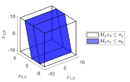
Figure 2: Set of admissible initial states: $x_{0}$ satisfying $M_{0}x_{0}\leq n_{0}$.

All simulations are executed with $x_{0}=\begin{bmatrix}-4.5&-2.6&-7\end{bmatrix}^{T}$ which is admissible.

The proposed control strategy is applied in a simulation with randomly generated realizations of $\mathbf{D}$, $\mathbf{H}$ and $\mathbf{S}$. These realizations and the resulting evolution of $x_{k}$ and $u_{k}$ are depicted in Fig. 3 which illustrates that applying the proposed control strategy satisfies all constraints on state an actuating variables while $x_{k}$ converges to zero with probability one.

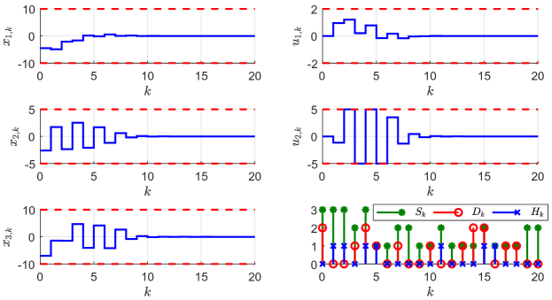
Figure 3: Simulation with randomly generated realizations of $\mathbf{D}$, $\mathbf{H}$ and $\mathbf{S}$.

The performance of the proposed stochastic MPC and the deterministic MPC from Section 3.2.5 minimizing the worst-case value of (7) are evaluated by comparing the evolution of

$$\tilde{J}_{k} =\sum\nolimits_{i=0}^{k}\left(x_{i}^{T}Qx_{i}+u_{i}^{T}Ru_{i}\right).$$ (68)

Three simulations are executed with $H_{k}=\overline{h}\ \forall\,k$: $(1)$ the stochastic MPC with $D_{k}=\overline{d}\ \forall\,k$ and $S_{k}=\overline{s}\ \forall\,k$; $(2)$ the stochastic MPC with $D_{k}=\underline{d}\ \forall\,k$ and $S_{k}=\underline{s}\ \forall\,k$; $(3)$ the deterministic MPC (which yields the same results for all possible realizations of $\mathbf{D}$ and $\mathbf{S}$). The resulting evolution of (68) is depicted in Fig. 4 which illustrates the potential increase in performance achieved by minimizing the expected value of the cost function instead of its worst-case value: $(i)$ the deterministic MPC is designed by minimizing $\tilde{J}_{\infty}$ for $D_{k}=\overline{d}\ \forall\,k$. Since this is not the only possible case, applying the proposed stochastic MPC results yields a larger cost if $D_{k}=\overline{d}\ \forall\,k$ actually holds. However, this difference is quite small. $(ii)$ if $D_{k}=\underline{d}\ \forall\,k$ and $S_{k}=\underline{s}\ \forall\,k$, applying the proposed stochastic MPC results in a significantly lower value of the cost function than minimizing its worst-case value.

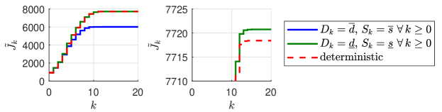
Figure 4: Comparing stochastic and deterministic MPC for $H_{k}=\overline{h}\ \forall\,k$.

6 Conclusion and Further Work

Compared to the MPC minimizing the worst-case value of the cost function, the proposed stochastic MPC $(i)$ potentially increases the performance significantly $(ii)$ without deteriorating the worst-case performance significantly $(iii)$ while guaranteeing feasibility for the same set of initial states.

However, the following issue has to be handled when considering real-world applications: for example, if $x_{k-1}$ and $x_{k}$ are known but $D_{k-1}$ is not, computing probabilities like in Section 4.1 utilizes the set of all $d_{k-1}$ for which $x_{k}=Ax_{k-1}+B\tilde{u}_{k-1-d_{k-1}}^{(d_{k-1})}$. This set will typically be empty when considering real-world applications where there is a mismatch between the plant and its model and therefore the set of possible values for $D_{k-1}$ is empty as well. While this can be handled by, for example, computing the set of all $d_{k-1}$ for which some norm of the difference between $x_{k}$ and $Ax_{k-1}+B\tilde{u}_{k-1-d_{k-1}}^{(d_{k-1})}$ is sufficiently small, including a suitable model of disturbances in the considered setup is considered to be the most important next step.

Appendix A

Due to (9), the sequence of actuating variables given by (20b) can be actually applied to the plant if it is possible to choose the controller output $\tilde{u}_{k+i}$ as

$$\tilde{u}_{k+i}^{(d)}=\begin{cases}\hat{u}_{k}^{(i+d)}&i+d\leq N-1\\ \kappa_{k}^{(i+d)}&N\leq i+d,\end{cases}\qquad\ d\in[\underline{d},\overline{d}]$$ (69)

for all $i\geq 0$. This is possible if $\kappa_{k}^{(N)}$ can be computed at at time step $k+N-\overline{d}$, if $\kappa_{k}^{(N+1)}$ can be computed at time step $k+N-\overline{d}+1$ and so on, i.e. it has to be possible to compute $\kappa_{k}^{(j)}$ at time step $k+j-\overline{d}$ for all $j\geq N$.

If $\kappa_{k}^{(l)}$ can be computed at time step $k+l-\overline{d}$ for all $l\in[N,j-1]$, which certainly holds for $j=N$, then $\tilde{u}_{k+i}^{(d)}$ can be computed via (69) for all $i\geq 0,\,d\in[\underline{d},\overline{d}]$ for which $i+d\leq j-1$. This results in

$$u_{k+l}=\tilde{u}_{k+l-D_{k+l}}^{(D_{k+l})}=\begin{cases}\hat{u}_{k}^{(l)}&D_{k+l}\leq l\leq N-1\\ \kappa_{k}^{(l)}&N\leq l\leq j-1\end{cases}$$ (70)

where $\kappa_{k}^{(l)}$ is known at time step $k+j-\overline{d}$ for all $l\in[N,j-1]$. It remains to be shown that this implies that it is also possible to compute $\kappa_{k}^{(j)}$ at time step $k+j-\overline{d}$ in order to show that it is possible to determine $\tilde{u}_{k+i}$ via (69) for all $i\geq 0$.

According to (21c),

$$\hat{H}_{k}^{(j)}+j=\min(\overline{h}+N-1,\overline{s}+N-2,\tilde{H}_{k}+j).$$

Since $\overline{h}\geq 0$ and $\overline{s}\geq 0$ and since $\tilde{H}_{k}\geq-1$ due to (21b),

$$\hat{H}_{k}^{(j)}+j=\min(\overline{h}+N-1,\overline{s}+N-2)\quad\forall\,j\geq N.$$

Since $N>\overline{d}\geq 1$, this yields $\hat{H}_{k}^{(j)}+j\geq 0$ for all $j\geq N$ so $x_{k+j}$ can be written as

$$x_{k+j}=A^{\hat{H}_{k}^{(j)}+j}x_{k-\hat{H}_{k}^{(j)}}+\sum\nolimits_{l=-\hat{H}_{k}^{(j)}}^{j-1}\!\!A^{j-1-l}Bu_{k+l}.$$

Inserting this result in (21a) yields

$$\kappa_{k}^{(j)}= -LA^{\hat{H}_{k}^{(j)}+j}x_{k-\hat{H}_{k}^{(j)}}-L\sum\nolimits_{l=\overline{d}}^{j-1}A^{j-1-l}Bu_{k+l}$$

$$-L\sum\nolimits_{l=-\hat{H}_{k}^{(j)}}^{\overline{d}-1}A^{j-1-l}B\mathbb{E}\left\{\left.u_{k+l}\right|\mathcal{I}_{k}\right\}.$$

Due to (70), $(u_{k+l})_{\overline{d}\leq l\leq j-1}$ is known at time step $k+j-\overline{d}$; since $k+j-\overline{d}>k$ for $j\geq N$, $\mathcal{I}_{k}$ is available as well.

$x_{k-\hat{H}_{k}^{(j)}}$ with $\hat{H}_{k}^{(j)}$ given by (21c) can be computed at time step $k+j-\overline{d}$ with $j\geq N$ as well since $(i)$ $x_{k-\tilde{H}_{k}}$ is known at time step $k<k+j-\overline{d}$ since $x_{k-H_{k}}$ is known and, if $k\geq K_{s}$, $\left(u_{\tilde{k}}\right)_{0\leq\tilde{k}\leq k-S_{k}}$ is also known, $(ii)$ $x_{k-\hat{H}_{k}^{(j)}}$ is known at time step $k+j-N+1$ if $\hat{H}_{k}^{(j)}=\overline{h}+N-j-1$, $(iii)$ $\left(u_{k+i}\right)_{-\tilde{H}_{k}\leq i\leq-(\hat{H}_{k}^{(j)}+1)}$ is known at time step $k+j-N+1$ if $\hat{H}_{k}^{(j)}=\overline{s}+N-j-2$ since then $k+j-N+1-S_{k+j-N+1}\geq k-(\hat{H}_{k}^{(j)}+1)$ and $(iv)$ if $x_{k-\hat{H}_{k}^{(j)}}$ can be computed at time step $k+j-N+1$ then it is also known at time step $k+j-\overline{d}$.

Therefore, $\kappa_{k}^{(j)}$ can be computed at time step $k+j-\overline{d}$ and therefore, (20b) can actually be applied to the plant for (21).

Appendix B

In order to show that $\kappa_{k+1}^{(N-1)}=-L\mathbb{E}\left\{\left.x_{k+N}\right|\mathcal{I}_{k+1}\right\}$ holds for (27), $x_{k+N}$ is written as
$A^{N+\hat{H}_{k+1}^{(N-1)}-1}x_{k+1-\hat{H}_{k+1}^{(N-1)}}+\sum\nolimits_{j=1-\hat{H}_{k+1}^{(N-1)}}^{N-1}A^{N-1-j}Bu_{k+j}$ where $\hat{H}_{k+1}^{(N-1)}=\tilde{H}_{k+1}$ due to (21c) so $x_{k+1-\hat{H}_{k+1}^{(N-1)}}$ can be computed from $\mathcal{I}_{k+1}$. For $j\in[\overline{d}+1,N-1]$, $\mathbb{E}\left\{\left.u_{k+j}\right|\mathcal{I}_{k+1}\right\}=u_{k+j}$ for (27) so $\mathbb{E}\left\{\left.x_{k+N}\right|\mathcal{I}_{k+1}\right\}-x_{k+N}=\sum\nolimits_{j=1-\hat{H}_{k+1}^{(N-1)}}^{\overline{d}}A^{N-1-j}B\left(\mathbb{E}\left\{\left.u_{k+j}\right|\mathcal{I}_{k+1}\right\}-u_{k+j}\right)$ so

$$\mathbb{E}\left\{\left.x_{k+N}\right|\mathcal{I}_{k+1}\right\}=x_{k+N}$$ (71)

$$+\sum\nolimits_{j=\hat{H}_{k+1}^{(N-1)}}^{\overline{d}-1}A^{N-2-j}B\left(\mathbb{E}\left\{\left.u_{k+1+j}\right|\mathcal{I}_{k+1}\right\}-u_{k+1+j}\right).$$

Computing $\kappa_{k+1}^{(N-1)}$ via (21a) and inserting $x_{k+N}$ from (71) yields $\kappa_{k+1}^{(N-1)}=-L\mathbb{E}\left\{\left.x_{k+N}\right|\mathcal{I}_{k+1}\right\}$.

Appendix C

In this Section it is shown that, for (29), (32) yields (33) with $\vec{d}_{k}\in\mathcal{D}_{k}$ for any $\vec{d}_{k+1}\in\mathcal{D}_{k+1}$. According to (21c),

$$\hat{H}_{k}^{(i)}=\min(\overline{h}+N-i-1,\overline{s}+N-i-2,\tilde{H}_{k})$$

$$\hat{H}_{k+1}^{(i-1)}-1=\min(\overline{h}+N-i,\overline{s}+N-i-1,\tilde{H}_{k+1})-1$$

$$\qquad\quad=\min(\overline{h}+N-i-1,\overline{s}+N-i-2,\tilde{H}_{k+1}-1).$$

Since $\tilde{H}_{k+1}\leq\tilde{H}_{k}+1$, i.e. since $\tilde{H}_{k+1}-1\leq\tilde{H}_{k}$, this implies that $(a)$ $\hat{H}_{k+1}^{(i-1)}-1\leq\hat{H}_{k}^{(i)}$ always holds and that $(b)$ if $\hat{H}_{k+1}^{(i-1)}-1<\tilde{H}_{k+1}-1$ then also $\hat{H}_{k}^{(i)}<\tilde{H}_{k}$ which results in $\hat{H}_{k+1}^{(i-1)}-1=\min(\overline{h}+N-i-1,\overline{s}+N-i-2)=\hat{H}_{k}^{(i)}$. This can be written as

$$\hat{H}_{k+1}^{(i-1)}-1<\tilde{H}_{k+1}-1\ \Rightarrow\ \hat{H}_{k+1}^{(i-1)}-1=\hat{H}_{k}^{(i)}$$ (72a)

$$\hat{H}_{k+1}^{(i-1)}-1=\tilde{H}_{k+1}-1\ \Rightarrow\ \hat{H}_{k+1}^{(i-1)}-1\leq\hat{H}_{k}^{(i)}.$$ (72b)

Due to (72a), (32) with $\hat{H}_{k+1}^{(i-1)}<\tilde{H}_{k+1}$ can be written as

$$\bar{\kappa}_{k+1}^{(i-1)}(\vec{d}_{k+1})=-Lx_{k+i}$$ (73)

$$\quad+L\sum\nolimits_{j=-\hat{H}_{k}^{(i)}}^{\overline{d}}A^{i-1-j}B\left(\bar{u}_{k}^{(j)}(D_{k+j})-\bar{u}_{k}^{(j)}(d_{k+j})\right).$$

Since $(x_{k+j})_{-k\leq j\leq 1-\tilde{H}_{k+1}}$ can be computed from $\mathcal{I}_{k+1}$ and $x_{k+j+1}-Ax_{k+j}=Bu_{k+j}$, $Bu_{k+j}$ can be computed from $\mathcal{I}_{k+1}$ for all $j\in[-k,-\tilde{H}_{k+1}]$. Due to (72b), this implies that $B\bar{u}_{k}^{(j)}(D_{k+j})=Bu_{k+j}$ can be computed from $\mathcal{I}_{k+1}$ for all $j\in-\hat{H}_{k}^{(i)}\leq j\leq-\hat{H}_{k+1}^{(i-1)}$ if $\hat{H}_{k+1}^{(i-1)}=\tilde{H}_{k+1}$. Therefore, $\mathbb{P}\left[\left.D_{k+j}\!=\!d_{k+j}\right|\mathcal{I}_{k+1}\right]=0$ if $B\bar{u}_{k}^{(j)}(d_{k+j})\neq B\bar{u}_{k}^{(j)}(D_{k+j})$ for all $j\in-\hat{H}_{k}^{(i)}\leq j\leq-\hat{H}_{k+1}^{(i-1)}$. Since $\vec{d}_{k+1}\in\mathcal{D}_{k+1}$ implies that $\mathbb{P}\left[\left.D_{k+j}=d_{k+j}\right|\mathcal{I}_{k+1}\right]>0$, this yields $B\big{(}\bar{u}_{k}^{(j)}(D_{k+j})-\bar{u}_{k}^{(j)}(d_{k+j})\big{)}=0$ for $\vec{d}_{k+1}\in\mathcal{D}_{k+1}$ so (73) also holds for $\hat{H}_{k+1}^{(i-1)}=\tilde{H}_{k+1}$ for all $\vec{d}_{k+1}\in\mathcal{D}_{k+1}$.

Inserting that, for (29), $\bar{u}_{k}^{(\overline{d})}(D_{k+\overline{d}})=\bar{u}_{k}^{(\overline{d})}(d_{k+\overline{d}})$ for any $d_{k+\overline{d}}\in[\underline{d},\overline{d}]$ in (73) yields $\bar{\kappa}_{k+1}^{(i-1)}(\vec{d}_{k+1})=\bar{\kappa}_{k}^{(i)}(\vec{d}_{k})$ according to (25b) where $\vec{d}_{k}\in\mathcal{D}_{k}$ since $(i)$ $\mathcal{D}_{k}$ is the set of all possible $\vec{D}_{k}$ given $\mathcal{I}_{k}$ and $(ii)$ if $\vec{D}_{k}=\vec{d}_{k}$ is possible given $\mathcal{I}_{k+1}$ then it is also possible given $\mathcal{I}_{k}\subseteq\mathcal{I}_{k+1}$.

Appendix D

Since $-\hat{H}_{k}^{(i)}\geq\overline{d}$ for all $i\geq\hat{N}$ as shown in Section 3.3.1, (37) yields $u_{k+i}=-Lx_{k+i}$ for all $i\geq\hat{N}$. Therefore, minimizing $\mathbb{E}\left\{\left.\sum\nolimits_{\tilde{k}=k+N}^{\infty}\left(x_{\tilde{k}}^{T}Qx_{\tilde{k}}+u_{\tilde{k}}^{T}Ru_{\tilde{k}}\right)\right|\mathcal{I}_{k+\alpha}\right\}$ with ${\alpha\in\mathbb{N}_{0}}$ with respect to $(v_{k+j})_{-\hat{H}^{(N)}_{k}\leq j\leq\overline{d}-1}$ subject to (37) where ${-\hat{H}^{(N)}_{k}\leq-\hat{H}^{(i)}_{k}}$ for all $i\geq N$ can be written as

$$\underset{(v_{k+j})_{-\hat{H}^{(N)}_{k}\leq j\leq\overline{d}-1}}{\min}\mathbb{E}\bigg{\{}\sum\nolimits_{\tilde{k}=N}^{\hat{N}-1}\left(x_{k+i}^{T}Qx_{k+i}+u_{k+i}^{T}Ru_{k+i}\right)$$

$$\qquad\qquad\qquad\qquad\qquad+x_{k+\hat{N}}^{T}Px_{k+\hat{N}}\Big{|}\mathcal{I}_{k+\alpha}\Big{\}}$$ (74)

$$s.t.\ u_{k+i}=-Lx_{k+i}+L\sum\nolimits_{j=-\hat{H}_{k}^{(i)}}^{\overline{d}-1}\!\!A^{i-1-j}B\left(u_{k+j}-v_{k+j}\right)$$

which can be written in the form

$$\underset{\check{v}_{k}}{\min}\ \mathbb{E}\left\{\left.\check{x}_{k}^{T}\check{Q}\check{x}_{k}+2\check{v}_{k}^{T}\check{H}\check{x}_{k}+\check{v}_{k}^{T}\check{R}\check{v}_{k}\right|\mathcal{I}_{k+\alpha}\right\}$$

$$\check{v}_{k}=\begin{bmatrix}v_{k+\overline{d}-1}\\ \vdots\\ v_{k-\hat{H}_{k}^{(N)}}\end{bmatrix},\quad\check{u}_{k}=\begin{bmatrix}u_{k+\overline{d}-1}\\ \vdots\\ u_{k-\hat{H}_{k}^{(N)}}\end{bmatrix},\quad\check{x}_{k}=\begin{bmatrix}x_{k+N}\\ \check{u}_{k}\end{bmatrix}$$

with $\check{R}=\check{R}^{T}\succeq 0$. Since $\check{x}_{k}$ is constant w.r.t. $\check{v}_{k}$ and since this optimization problem is convex, $\check{v}_{k}=\check{v}_{k}^{*}$ is optimal if

$$\check{R}\check{v}_{k}^{*}+\check{H}\mathbb{E}\left\{\left.\check{x}_{k}\right|\mathcal{I}_{k+\alpha}\right\}=0.$$ (75)

In order to show that $v_{k+j}^{*}=\mathbb{E}\left\{\left.u_{k+j}\right|\mathcal{I}_{k+\alpha}\right\}$ is optimal, it remains to be shown that (75) holds for

$$\check{v}_{k}^{*} =\mathbb{E}\left\{\left.\check{u}_{k}\right|\mathcal{I}_{k+\alpha}\right\}=\begin{bmatrix}0&I\end{bmatrix}\mathbb{E}\left\{\left.\check{x}_{k}\right|\mathcal{I}_{k+\alpha}\right\}.$$ (76)

This certainly holds if $\alpha$ is large enough such that $\mathbb{E}\left\{\left.\check{x}_{k}\right|\mathcal{I}_{k+\alpha}\right\}=\check{x}_{k}$ since $\check{v}_{k}=\check{u}_{k}$ results in $u_{k+i}=-Lx_{k+i}$ for all $i\geq N$ which minimizes (74). In other words, $\check{R}\begin{bmatrix}0&I\end{bmatrix}\check{x}_{k}+\check{H}\check{x}_{k}=0$ holds for any possible $\check{x}_{k}$.

While $\check{x}_{k}$ is not known for smaller values of $\alpha$,

$$\check{R}\begin{bmatrix}0&I\end{bmatrix}\check{x}_{k}+\check{H}\check{x}_{k}=0\text{ for all possible $\check{x}_{k}$ }$$

$$\qquad\Rightarrow\check{R}\begin{bmatrix}0&I\end{bmatrix}\mathbb{E}\left\{\left.\check{x}_{k}\right|\mathcal{I}_{k+\alpha}\right\}+\check{H}\mathbb{E}\left\{\left.\check{x}_{k}\right|\mathcal{I}_{k+\alpha}\right\}=0$$

and therefore (75) holds for (76) for all ${\alpha\in\mathbb{N}_{0}}$.

Appendix E

E.1 Definitions

$$\tilde{P}_{1}(\underline{i},\overline{i},\delta_{\underline{i}},(\Theta_{i})_{\underline{i}+1\leq i\leq\overline{i}})$$ (77)

$$\qquad\qquad\qquad=\mathbb{P}\left[\left.D_{i}\in\Theta_{i}\,\forall\,i\in[\underline{i}+1,\overline{i}]\right|D_{\underline{i}}=\delta_{\underline{i}}\right]$$

for $\overline{i}>\underline{i}$ which can be written as (44a) using (4) and (5b).

$$\tilde{P}_{2}(\underline{i},\overline{i},\delta_{\underline{i}},\delta_{\overline{i}},(\Theta_{i})_{\underline{i}+1\leq i\leq\overline{i}-1})$$

$$\qquad=\mathbb{P}\left[\left.D_{\overline{i}}=\delta_{\overline{i}}\right|D_{\underline{i}}=\delta_{\underline{i}},\,D_{i}\in\Theta_{i}\,\forall\,i\in[\underline{i}+1,\overline{i}-1]\right]$$

$$\qquad=\frac{\mathbb{P}\left[\left.D_{\overline{i}}=\delta_{\overline{i}},\,D_{i}\in\Theta_{i}\,\forall\,i\in[\underline{i}+1,\overline{i}-1]\right|D_{\underline{i}}=\delta_{\underline{i}}\right]}{\mathbb{P}\left[\left.D_{i}\in\Theta_{i}\,\forall\,i\in[\underline{i}+1,\overline{i}-1]\right|D_{\underline{i}}=\delta_{\underline{i}}\right]}$$

for $\underline{i}+1\leq\overline{i}-1$ using the definition of conditional probability. Using (77), this can be written as (44b).

$$\tilde{P}_{3}(\underline{i},\overline{i},(\Theta_{i})_{\underline{i}\leq i\leq\overline{i}})=\mathbb{P}\left[D_{i}\in\Theta_{i}\,\forall\,i\in[\underline{i},\overline{i}]\right]=$$ (78)

$$\sum\nolimits_{d_{0}=\underline{d}}^{\overline{d}}\mathbb{P}\left[D_{0}=d_{0}\right]\mathbb{P}\left[\left.D_{i}\in\Theta_{i}\,\forall\,i\in[\underline{i},\overline{i}]\right|D_{0}=d_{0}\right]=$$

$$\begin{cases}\sum\limits_{d_{0}\in\Theta_{0}}\mu(d_{0})&0=\underline{i}=\overline{i}\\ \sum\limits_{d_{0}\in\Theta_{0}}\mu(d_{0})\mathbb{P}\left[\left.D_{i}\in\Theta_{i}\,\forall\,i\in[1,\overline{i}]\right|D_{0}=d_{0}\right]&0=\underline{i}<\overline{i}\\ \sum\nolimits_{d_{0}=\underline{d}}^{\overline{d}}\mu(d_{0})\sum\nolimits_{d_{\underline{i}}\in\Theta_{\underline{i}}}\mathbb{P}\left[\left.D_{\underline{i}}=d_{\underline{i}}\right|D_{0}=d_{0}\right]&0<\underline{i}=\overline{i}\\ \begin{matrix}\sum\nolimits_{d_{0}=\underline{d}}^{\overline{d}}\mu(d_{0})\sum\nolimits_{d_{\underline{i}}\in\Theta_{\underline{i}}}\mathbb{P}\left[\left.D_{\underline{i}}=d_{\underline{i}}\right|D_{0}=d_{0}\right]\\ \mathbb{P}\left[\left.D_{i}\in\Theta_{i}\,\forall\,i\in[\underline{i}+1,\overline{i}]\right|D_{\underline{i}}=d_{\underline{i}}\right]\end{matrix}&0<\underline{i}<\overline{i}\end{cases}$$

for $\underline{i}\leq\overline{i}$ using the law of total probability and (5a). Using (6), this can be written as (44c). $\tilde{P}_{4}(\underline{i},\overline{i},\delta_{\overline{i}},(\Theta_{i})_{\underline{i}\leq i\leq\overline{i}-1})=$

$$\mathbb{P}\left[\left.D_{\overline{i}}=\delta_{\overline{i}}\right|D_{i}\in\Theta_{i}\,\forall\,i\in[\underline{i},\overline{i}-1]\right]$$

$$=\frac{\mathbb{P}\left[D_{\overline{i}}=\delta_{\overline{i}},\,D_{i}\in\Theta_{i}\,\forall\,i\in[\underline{i},\overline{i}-1]\right]}{\mathbb{P}\left[D_{i}\in\Theta_{i}\,\forall\,i\in[\underline{i},\overline{i}-1]\right]}$$

for $\underline{i}\leq\overline{i}-1$ which can be written as (44d) using (78).

E.2 Probabilities

E.2.1 $\mathit{k\geq K_{sd}}$

For $\tilde{h}_{k}=s_{k}-1$, (43) can be written as

$$P_{k}(\delta)=\mathbb{P}\left[\left.D_{k-s_{k}+1}=\delta\right|D_{k-s_{k}}=d_{k-s_{k}}\right]=\Phi(d_{k-s_{k}},\delta)$$

using (5b). For $\tilde{h}_{k}<s_{k}-1$, (43) can be written as

$$P_{k}(\delta)=\mathbb{P}\big{[}D_{k-\tilde{h}_{k}}=\delta\big{|}D_{k-s_{k}}=d_{k-s_{k}},$$

$$\qquad\qquad\qquad D_{k+i}\in\Theta_{k,i}\,\forall\,i\in[-s_{k}+1,-\tilde{h}_{k}-1]\big{]}$$

$$=\tilde{P}_{2}(k-s_{k},k-\tilde{h}_{k},d_{k-s_{k}},\delta,(\Theta_{k,i})_{-s_{k}+1\leq i\leq-\tilde{h}_{k}-1}).$$

E.2.2 $\mathit{k<K_{s}}$

For $k-\tilde{h}_{k}\leq\underline{d}$, (43) can be written as

$$P_{k}(\delta)=\mathbb{P}\big{[}D_{k-\tilde{h}_{k}}=\delta\big{]}=\sum\nolimits_{d_{0}=\underline{d}}^{\overline{d}}\mu(d_{0})\Phi_{k-\tilde{h}_{k}}(d_{0},\delta)$$ (79)

using (6). For $k-\tilde{h}_{k}>\underline{d}$, (43) can be written as

$$P_{k}(\delta)=\mathbb{P}\big{[}D_{k-\tilde{h}_{k}}=\delta\big{|}D_{k+i}\in\Theta_{k,i}\,\forall\,i\in[\underline{d}-k,-\tilde{h}_{k}-1]\big{]}$$

$$=\tilde{P}_{4}(\underline{d},k-\tilde{h}_{k},\delta,(\Theta_{k,i})_{\underline{d}-k\leq i\leq-\tilde{h}_{k}-1}).$$

E.2.3 $\mathit{K_{s}\leq k<K_{sd}}$

For $k-\tilde{h}_{k}\leq\underline{d}$, (43) can be written as (79). For $k-\tilde{h}_{k}>\underline{d}$, (43) yields

$$P_{k}(\delta)=\mathbb{P}\big{[}D_{k-\tilde{h}_{k}}=\delta\big{|}D_{k+i}\in\hat{\Theta}_{k,i}\,\forall\,i\in[\underline{d}-k,-\tilde{h}_{k}-1]\big{]}$$

$$=\tilde{P}_{4}\big{(}\underline{d},k-\tilde{h}_{k},\delta,(\hat{\Theta}_{k,i})_{\underline{d}-k\leq i\leq-\tilde{h}_{k}-1}\big{)}.$$

References

- [1] D.Q. Mayne et al. “Constrained model predictive con- trol: Stability and optimality”. In: Automatica 36.6 (2000), pp. 789–814.
- [2] M. Reble, D. E. Quevedo, and F. Allgöwer. “Control over erasure channels: stochastic stability and perfor- mance of packetized unconstrained model predictive control”. In: International Journal of Robust and Non- linear Control 23.10 (2013), pp. 1151–1167.
- [3] D. E. Quevedo and D. Nešić. “On Stochastic Stability of Packetized Predictive Control of Non-linear Systems over Erasure Channels”. In: IFAC Proceedings Volumes 43.14 (2010). 8th IFAC Symposium on Nonlinear Con- trol Systems, pp. 557–562.
- [4] P. K. Mishra, D. Chatterjee, and D. E. Quevedo. “Stochastic predictive control under intermittent ob- servations and unreliable actions”. In: Automatica 118 (2020), p. 109012.
- [5] P. Li et al. “Packet-Based Model Predictive Control for Networked Control Systems With Random Packet Losses”. In: 2018 IEEE Conference on Decision and Control (CDC). 2018, pp. 3457–3462.
- [6] J. Wu, L. Zhang, and T. Chen. “Model predictive con- trol for networked control systems”. In: International Journal of Robust and Nonlinear Control 19.9 (2009), pp. 1016–1035.
- [7] M. Palmisano, M. Steinberger, and M. Horn. “Optimal Finite-Horizon Control for Networked Control Systems in the Presence of Random Delays and Packet Losses”. In: IEEE Control Systems Letters 5.1 (2021), pp. 271– 276.
- [8] E. G. Gilbert and K. T. Tan. “Linear systems with state and control constraints: the theory and application of maximal output admissible sets”. In: IEEE Transactions on Automatic Control 36.9 (1991), pp. 1008–1020.
- [9] S. Keerthi and E. Gilbert. “Computation of minimum- time feedback control laws for discrete-time systems with state-control constraints”. In: IEEE Transactions on Automatic Control 32.5 (1987), pp. 432–435.
- [10] M. Herceg et al. “Multi-Parametric Toolbox 3.0”. In: 2013 European Control Conference (ECC). 2013, pp. 502–510.