Synthesis of Ballistic Capture Corridors at Mars via Polynomial Chaos Expansion

1 Introduction

The space sector is experiencing a flourishing growth. Evidence is mounting that the near future will be characterized by a large amount of deep-space missions [1, 2, 3, 4]. In the last decade, CubeSats have granted affordable access to space due to their reduced manufacturing costs compared to traditional missions. Nowadays, most miniaturized spacecraft have thus far been deployed into near-Earth orbits, but soon a multitude of interplanetary CubeSats will be employed for deep-space missions as well [5]. Nevertheless, the current paradigm for deep-space missions strongly relies on ground-based operations [6]. Although reliable, this approach will rapidly cause saturation of ground slots, thereby hampering the current momentum in space exploration. At the actual pace, human-in-the-loop, flight-related operations for deep-space missions will soon become unsustainable.

Self-driving spacecraft challenge the current paradigm under which spacecraft are piloted in interplanetary space. They are intended as machines capable of traveling in deep space and autonomously reaching their destination. In EXTREMA (short for Engineering Extremely Rare Events in Astrodynamics for Deep-Space Missions in Autonomy) [5, 7], these systems are used to engineer ballistic capture (BC) [8, 9, 10], thereby proving the effectiveness of autonomy in a complex scenario. The BC mechanism allows capture about a planet exploiting the natural dynamics, thus without requiring maneuvers [11, 12, 13, 14]. At the expense of longer transfer times, BC orbits are cheaper, safer, and more versatile from the operational perspective than Keplerian solutions [11]. Furthermore, BC is a desirable solution for limited-control platforms, which cannot afford to enter into orbits about a planet due to a lack of significant control authority. The key is to accomplish low-thrust orbits culminating in BC. For this, a bundle of BC orbits named ballistic capture corridor (BCC) can be targeted far away from a planet [15, 16, 17]. Mars is chosen in this work due to its relevance in the long-term exploration [5].

BC is an extremely rare event, thus massive numerical simulations are required to find the specific conditions supporting capture. On average, only 1 out of $10\,000$ conditions explored by algorithms grants capture [18]. To achieve BC at Mars without any a priori instruction, an inexpensive and accurate method to construct BCC directly on board is required. Therefore, granting spacecraft the capability to manipulate stable sets in order to compute autonomously BCC is crucial [15]. The goal of the paper is to numerically synthesize a corridor exploiting the polynomial chaos expansion (PCE) technique, thereby applying a suited uncertainty propagation technique to BC orbit propagation. In the literature, PCE was introduced and exploited for uncertainty quantification [19, 20]. PCE can be used as an effective interpolation method, avoiding a priori definition of interpolant functions but selecting them automatically starting from the input samples, so that they possess spectral convergence with respect to the input variables. Furthermore, proving it to be successful in propagating all-in-once a bundle of trajectories in a deterministic setting opens the door to a wider use for PCE in data-driven approaches [21]. The proposed approach is validated against Monte Carlo (MC) simulation. The heavy computational loads derived by multiple point-wise propagations of BC orbits when performing guidance and control tasks during the low-thrust interplanetary cruise are unburdened by the devised methodology. Broadly, this will facilitate the paradigm shift towards autonomy, thereby favoring the reduction of mission load on ground stations by decreasing the demand foreseen in the next years.

The remainder of the paper is organized as follows. In Section 2, the background is introduced. Then, the proposed methodology follows in Section 3. Results are presented in Section 4. Eventually, conclusions are drawn in Section 5.

2 Background

2.1 Dynamical model

Following the nomenclature in [9], a target and a primary are defined. The target is the body around which BC is studied. The primary is the main body around which the target revolves. Target and primary masses are $m_{t}$ and $m_{p}$, respectively. The mass ratio of the system is $\mu=m_{t}/(m_{t}+m_{p})$. This work focuses on BC having Mars as target and the Sun as primary. Reference frames used in this work are the J2000 and RTN@$t_{i}$ [22].

The precise states of the Sun and the major planets are retrieved from the Jet Propulsion Laboratory (JPL)’s planetary ephemerides de440s.bsp (or DE440s) [23]. Additionally, the ephemerides mar097.bsp of Mars (the target) and its moons are employed. The following generic leap seconds kernel (LSK) and planetary constant kernel (PCK) are used: naif0012.tls, pck00010.tpc, and gm_de440.tpc.

The Equations of motion (EoM) of the restricted $n$-body problem are considered. The gravitational attractions of the Sun, Mercury, Venus, Earth–Moon (B), Mars (central body), Jupiter (B), Saturn (B), Uranus (B), and Neptune (B) are taken into account. Additionally, solar radiation pressure (SRP), Mars’ non-spherical gravity (NSG), and relativistic corrections [24] are considered. Table 1 collects the assumed spacecraft parameters needed to evaluate the SRP perturbation. They are compatible with those of a 12U deep-space CubeSat [25]. Terms of the infinite series modeling NSG are considered up to degree $n_{\mathrm{deg}}=$20\text{\,}$$ and order $n_{\mathrm{ord}}=$20\text{\,}$$ [17]. The coefficients to evaluate the NSG perturbation are retrieved from the MRO120F gravity field model of Mars. Data are publicly available in the file jgmro_120f_sha.tab, archived in the Geosciences Node of NASA’s Planetary Data System. Far from Mars, when in heliocentric motion, the NSG perturbation is neglected. EoM are integrated in the J2000 inertial frame.

Table 1: Spacecraft parameters for SRP evaluation [25].

Parameter	Unit	Value
Mass–SRP area ratio $m/A$	$\mathrm{kg}\text{\,}{\mathrm{m}}^{-2}$	$75\text{\,}$
Coefficient of reflectivity $C_{r}$	-	$1.3\text{\,}$

The EoM in a non-rotating Mars-centered reference frame are [9, 26, 24]

$$\begin{split}\ddot{\mathbf{r}}=&-\frac{\mu_{t}}{r^{3}}\mathbf{r}-\sum\limits_{i\in\mathbb{P}}\mu_{i}\left(\frac{\mathbf{r}_{i}}{r_{i}^{3}}+\frac{\mathbf{r}-\mathbf{r}_{i}}{\left\lVert\mathbf{r}-\mathbf{r}_{i}\right\rVert^{3}}\right)+\frac{QA}{m}\frac{\mathbf{r}-\mathbf{r}_{\odot}}{\left\lVert\mathbf{r}-\mathbf{r}_{\odot}\right\rVert^{3}}-\mathcal{R}\frac{\mu_{t}}{r^{2}}\left(\Lambda\frac{\mathcal{R}^{\top}\mathbf{r}}{r}-\left[J^{\top}\ K^{\top}\ H^{\top}\right]^{\top}\right)+\\ &+\frac{\mu_{t}}{c^{2}r^{3}}\left[\left(4\frac{\mu_{t}}{r}-v^{2}\right)\mathbf{r}+4\left(\mathbf{r}\cdot\dot{\mathbf{r}}\right)\dot{\mathbf{r}}\right]+2\left(\mathbf{\Omega}\times\dot{\mathbf{r}}\right)+2\frac{\mu_{t}}{c^{2}r^{3}}\left[\frac{3}{r^{2}}\left(\mathbf{r}\times\dot{\mathbf{r}}\right)\left(\mathbf{r}\cdot\mathbf{J}\right)+\left(\dot{\mathbf{r}}\times\mathbf{J}\right)\right]\end{split}$$ (1)

where $\mu_{t}$ is the gravitational parameter of the target body (i. e., Mars in this work); $\mathbf{r}$ and $\dot{\mathbf{r}}=\mathbf{v}$ are the position and velocity vectors of the spacecraft with respect to the target, respectively, being $r$ and $v$ their magnitudes; $\mathbb{P}$ is a set of $n-2$ indexes (where $n$ concerns the $n$-body problem) each one referring to the perturbing bodies; $\mu_{i}$ and $\mathbf{r}_{i}$ are the gravitational parameter and position vector of the $i$-th body with respect to the target, respectively; $A$ is the Sun-projected area on the spacecraft for SRP evaluation; $m$ is the spacecraft mass; $\mathbf{r}_{\odot}$ is the position vector of the Sun with respect to the target; $\mathcal{R}$ is the time-dependent matrix transforming vector components from the Mars-fixed frame to the non-rotating frame in which the EoM are written; $\Lambda$, $J$, $K$, and $H$ are defined as in [27]; $c=$299\,792\,458\text{\,}\mathrm{m}\text{\,}{\mathrm{s}}^{-1}$$ (from SPICE [28, 29]) is the speed of light in vacuum; $\mathbf{J}$ is the rotating central body’s angular momentum per unit mass in the J2000 frame. Then, $Q=LC_{r}/\left(4\pi c\right)$ where $C_{r}$ is the spacecraft coefficient of reflectivity, and $L=S_{\odot}4\pi d_{\mathrm{AU}}^{2}$ is the luminosity of the Sun. The latter is computed from the solar constant $S_{\odot}=$1367.5\text{\,}\mathrm{W}\text{\,}{\mathrm{m}}^{-2}$$ evaluated at $d_{\mathrm{AU}}=$1\text{\,}\mathrm{AU}$$. Lastly, $\mathbf{\Omega}=\tfrac{3}{2}\dot{\mathbf{r}}_{\odot/t}\times\left(-\mu_{\odot}\mathbf{r}_{\odot/t}\right)/\left(c^{2}r_{\odot/t}^{3}\right)$ where $\mu_{\odot}$ is the gravitational parameter of the Sun; $\mathbf{r}_{\odot/t}$ and $\dot{\mathbf{r}}_{\odot/t}=\mathbf{v}_{\odot/t}$ are the position and velocity vectors, respectively, of the target body with respect to the Sun, being $r_{\odot/t}$ and $\dot{r}_{\odot/t}=v_{\odot/t}$ their magnitudes.

The EoM in Eq. (1) are integrated with the GRavity TIdal Slide (GRATIS) tool [30] in their nondimensional form to avoid ill-conditioning (see normalization units in Table 2) [9]. Numerical integration is carried out with the DOPRI8 propagation scheme [31, 32]. The dynamics are propagated with relative and absolute tolerances set to $\mathrm{10^{-13}}$ [9].

Table 2: Nondimensionalization units.

Unit	Symbol	Value	Comment
Gravity parameter	$\mathrm{MU}$	$42\,828.376\text{\,}{\mathrm{km}}^{3}\text{\,}{\mathrm{s}}^{-2}$	Mars’ gravity parameter $\mu_{t}$
Length	$\mathrm{LU}$	$3396.0000\text{\,}\mathrm{km}$	Mars’ radius $R_{\mars}$
Time†	$\mathrm{TU}$	$956.281\,42\text{\,}\mathrm{s}$	$(\mathrm{LU}^{3}/\mathrm{MU})^{0\!.5}$
Velocity	$\mathrm{VU}$	$3.551\,255\,8\text{\,}\mathrm{km}\text{\,}{\mathrm{s}}^{-1}$	$\mathrm{LU}/\mathrm{TU}$

• Time unit chosen such that the nondimensional period of a circular orbit of radius $\mathrm{LU}$ equals $$2$\pi$.

2.2 Ballistic capture corridors

BC orbits are characterized by initial conditions (ICs) escaping the target when integrated backward and performing $n$ revolutions about it when propagated forward, neither impacting nor escaping the target. In forward time, particles flying on BC orbits approach the target coming from outside its sphere of influence and remain temporarily captured about it. After a certain time, the particle escapes if an energy dissipation mechanism does not take place to make the capture permanent. To dissipate energy either a breaking maneuver or the target atmosphere (if available) could be used [33, 34]. Effects on BC by gravitational attractions of many bodies besides the primaries and SRP have been investigated in previous works [35, 17, 36, 18].

A particle stability is inferred using a plane in the three-dimensional physical space [12], this according to the spatial stability definition provided in [9]. Based on its dynamical behavior, a propagated trajectory is said to be: i) weakly stable (sub-set $\mathcal{W}_{i}$) if the particle performs $i$ complete revolutions around the target neither escaping nor impacting with it or its moons; ii) unstable (sub-set $\mathcal{X}_{i}$) if the particle escapes from the target before completing the $i$th revolution; iii) target–crash (sub-set $\mathcal{K}_{i}$) if the particle impacts with the target before completing the $i$th revolution; iv) moon–crash (sub-set $\mathcal{M}_{i}$) if the particle impacts with one of the target’s moons before completing the $i$th revolution; v) acrobatic (sub-set $\mathcal{D}_{i}$) if none of the previous conditions occurs within the integration time span. Conditions ii)-v) apply after the particle performs $(i-$1\text{\,}$)$ revolutions around the target (see Fig. 1). The sub-sets are defined for $i\in\mathbb{Z}\textbackslash\{0\}$, where the sign of $i$ informs on the propagation direction. When $i>0$ ($i<0$) the IC is propagated forward (backward) in time. A capture set is defined as $\mathcal{C}_{-1}^{n}:=\mathcal{W}_{n}\cap\mathcal{X}_{-1}$. Therefore, it is the intersection between the stable set in forward time $\mathcal{W}_{n}$ and the unstable set in backward time $\mathcal{X}_{-1}$ [9].

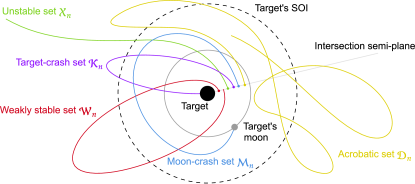
Figure 1: Illustration of particle stability. Weakly stable set $\mathcal{W}_{n}$ in red, unstable set $\mathcal{X}_{n}$ in green, target-crash set $\mathcal{K}_{n}$ in purple, moon-crash set $\mathcal{M}_{n}$ in blue, and acrobatic set $\mathcal{D}_{n}$ in yellow. Example with $n=$1$$. The points on the intersection semi-plane are the ICs.

BCCs are time-varying manifolds supporting capture [15] obtained backward propagating ICs belonging to a capture sets $\mathcal{C}_{-1}^{n}$, where $n>0$ is the number of revolutions after capture. They are defined in what follows. Firstly, a trajectory is defined as:

Definition 1

Let $(\mathbf{x}_{0},t_{0})\in\mathbb{R}^{6}\times\mathbb{R}$ and ${\bm{\varphi}}(\mathbf{x}_{0},t_{0};t)$ be the starting point and the solution at time $t$, respectively, of the state-space representation $\dot{\mathbf{x}}=\mathbf{f}(\mathbf{x},t)$ of the EoM in Eq. (1). Then, a trajectory $\gamma$ is defined as $\gamma(\mathbf{x}_{0},t_{0}):=\{\bm{\varphi}(\mathbf{x}_{0},t_{0};t)\ \forall t\in\mathbb{R}\}$. Similarly, backward and forward legs $\gamma_{b}$ and $\gamma_{f}$, respectively, are defined as $\gamma_{b}(\mathbf{x}_{0},t_{0}):=\{\bm{\varphi}(\mathbf{x}_{0},t_{0};t)\ \forall t\in[t_{0}-$10$T_{\mars},\,t_{0}]\}$ and $\gamma_{f}(\mathbf{x}_{0},t_{0}):=\{\bm{\varphi}(\mathbf{x}_{0},t_{0};t)\ \forall t\in[t_{0},\,t_{0}+$10$T_{\mars}]\}$, where $T_{\mars}=2\pi\sqrt{a_{\mars}^{3}/\mu_{\odot}}=$687\text{\,}\mathrm{days}$$ is the revolution period of Mars, with $a_{\mars}=$2.279\text{\times}{10}^{8}\text{\,}\mathrm{km}$$ and $\mu_{\odot}=$1.327\text{\times}{10}^{11}\text{\,}{\mathrm{km}}^{3}\text{\,}{\mathrm{s}}^{-2}$$ the semi-major axis of the Sun–Mars system and the gravitational parameter of the Sun, respectively.

Sets $\Gamma_{\mathcal{W}_{n}}$, $\Gamma_{\mathcal{X}_{-1}}$, and $\Gamma_{\mathcal{C}_{-1}^{n}}$ of trajectories $\gamma(\mathbf{x}_{0},t_{0})$ whose ICs $(\mathbf{x}_{0},t_{0})$ belong to weakly-stable set $\mathcal{W}_{n}$, escape set $\mathcal{X}_{-1}$, and capture set $\mathcal{C}_{-1}^{n}$, respectively, are $\Gamma_{\mathcal{W}_{n}}=\{\gamma(\mathbf{x}_{0},t_{0})\ \forall\,(\mathbf{x}_{0},t_{0})\in\mathcal{W}_{n}\}$, $\Gamma_{\mathcal{X}_{-1}}=\{\gamma(\mathbf{x}_{0},t_{0})\ \forall\,(\mathbf{x}_{0},t_{0})\in\mathcal{X}_{-1}\}$, and $\Gamma_{\mathcal{C}_{-1}^{n}}=\{\gamma(\mathbf{x}_{0},t_{0})\ \forall\,(\mathbf{x}_{0},t_{0})\in\mathcal{C}_{-1}^{n}\}$. Similarly to a capture set $\mathcal{C}_{-1}^{n}$, a corridor is designated is defined as $\mathcal{\check{B}}_{-1}^{n}=\{\gamma_{b}(\mathbf{x}_{0},t_{0})\ \forall\,(\mathbf{x}_{0},t_{0})\in\mathcal{C}_{-1}^{n}\}$. An exterior corridor $\mathcal{\check{E}}_{-1}^{n}$ is a subset of a corridor $\mathcal{\check{B}}_{-1}^{n}$ including pre-capture trajectories having heliocentric semi-major axis $a_{\odot}$ greater than the target body’s one (i. e., Mars, whose semi-major axis $a_{t}=a_{\mars}=$1.5237\text{\,}\mathrm{AU}$$). It is defined as $\mathcal{\check{E}}_{-1}^{n}=\{\gamma_{b}(\mathbf{x}_{0},t_{0})\in\mathcal{\check{B}}_{-1}^{n}:a_{\odot}\left(\bm{\varphi}(\mathbf{x}_{0},t_{0};t)\right)>a_{t}\ \forall t\in[t_{0}-$10$T_{\mars},\,\hat{t}]\}$ where $\hat{t}<t_{0}$ is a certain time before capture epoch $t_{0}$ when the escape (or pre-capture) leg ends in backward time. Contrarily, an interior corridor $\mathcal{\check{I}}_{-1}^{n}$ is the subset of a corridor $\mathcal{\check{B}}_{-1}^{n}$ including all trajectories having semi-major axis smaller than the central body’s one (i. e., Mars). It is defined as $\mathcal{\check{I}}_{-1}^{n}=\{\gamma_{b}(\mathbf{x}_{0},t_{0})\in\mathcal{\check{B}}_{-1}^{n}:a_{\odot}\left(\bm{\varphi}(\mathbf{x}_{0},t_{0};t)\right)<a_{t}\ \forall t\in[t_{0}-$10$T_{\mars},\,\hat{t}]\}$. Consequently, $\mathcal{\check{B}}_{-1}^{n}=\mathcal{\check{E}}_{-1}^{n}\cup\mathcal{\check{I}}_{-1}^{n}$.

In this work, the interior corridor is of interest because it extends between Mars and Earth’s orbits. A subcorridor $\mathcal{\check{S}}_{-1}^{n}$, a generic subset of a corridor $\mathcal{\check{B}}_{-1}^{n}$, is defined as $\mathcal{\check{S}}_{-1}^{n}=\{\gamma_{b}(\mathbf{x}_{0},t_{0})\ \forall\,(\mathbf{x}_{0},t_{0})\in\mathcal{D}_{-1}^{n}\}$, where the generic domain is $\mathcal{D}_{-1}^{n}=\{\mathbf{x}_{0}:\mathbf{x}_{0}\in\mathcal{C}_{-1}^{n}\wedge\mathbf{g}(\mathbf{x}_{0})\leq\mathbf{0}\wedge\mathbf{h}(\mathbf{x}_{0})=\mathbf{0}\}$, with $\mathbf{g}(\mathbf{x}_{0})$ and $\mathbf{h}(\mathbf{x}_{0})$ being two sets of $m\geq 0$ inequality constraints and $n\geq 0$ equality constraints, respectively, with $m$ and $p$ finite. Finally, the envelope $\mathcal{\partial\check{S}}_{-1}^{n}$ of a subcorridor $\mathcal{\check{S}}_{-1}^{n}$ is constructed backward propagating the subcorridor domain border $\partial\mathcal{D}_{-1}^{n}$. Therefore, it is defined as $\partial\mathcal{\check{S}}_{-1}^{n}=\{\gamma_{b}(\mathbf{x}_{0},t_{0})\ \forall\,(\mathbf{x}_{0},t_{0})\in\partial\mathcal{D}_{-1}^{n}\}$. An illustration of prior definitions is proposed in Fig. 2.

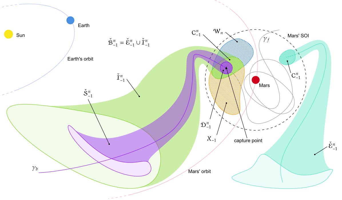
Figure 2: Illustration of BCC definitions.

2.3 Polynomial chaos expansion

PCE is an uncertain quantification method able to provide an efficient mean for long term propagation of non-Gaussian distributions. PCE approximates the stochastic solution of the governing dynamics as a weighted sum of multivariate spectral polynomials, function of the input random variables [20]

$$\bm{x}(t,\bm{\xi})\approx\hat{\bm{x}}(t,\bm{\xi})=\sum_{\bm{\alpha}\in\Lambda_{p,d}}\bm{c}_{\bm{\alpha}}(t)\psi_{\bm{\alpha}}(\bm{\xi})$$ (2)

where $\bm{\xi}\in\mathbb{R}^{d}$ is the random input vector, $\bm{c}_{\bm{\alpha}}(t)$ is the vector of polynomial chaos coefficients (PCCs), and $\Lambda_{p,d}$ is the set of multi-indices of size $d$ and order $p$, having so a total dimension equal to [20]

$$P=|\Lambda_{p,d}|=\dfrac{(p+d)!}{p!\,d!}.$$ (3)

Namely, $\bm{c}_{\bm{\alpha}}(t)\in\mathbb{R}^{n}$, where $n$ is the number of quantities of interest. If considering the full state propagation, $\bm{x}$ represents both the position and velocity and, hence, $n=6$.

The basis functions $\psi_{\bm{\alpha}}(\bm{\xi})$ are multidimensional spectral polynomials, orthonormal with respect to the joint probability measure of the vector $\bm{\xi}$. Thus, the basis functions choice depends only on the properties of the input variables. For example, Hermite and Legendre polynomials are the basis for the Gaussian and uniform distributions, respectively [37].

Generating a PCE means computing the PCCs by projecting the exact solution onto each basis function $\psi_{\bm{\alpha}}(\bm{\xi})$ [20]

$$\bm{c_{\alpha}}(t)=\mathit{E}[\bm{x}(t,\cdot)\psi_{\bm{\alpha}}(\cdot)]=\int_{\Gamma^{d}}\bm{x}(t,\bm{\xi})\psi_{\bm{\alpha}}(\bm{\xi})\rho(\bm{\xi})d\bm{\xi}$$ (4)

where $\Gamma^{d}$ is the $d$-dimensional hypercube where the random input variables are defined. Once the PCCs are computed, the system state associated to a specific sample within the capture subset can be retrieved at time $t$ effortlessly using Eq. (2). The PCCs estimation methods fall into two categories: intrusive and non-intrusive. While the first requires laborious modifications in the governing equations, the latter treat the dynamics as a black box, thus they are better suited for problems with high-fidelity complex dynamics [19].

3 Methodology

3.1 Problem statement

The goal of the BCC synthesis is to produce a numerical approximation of a subcorridor. The approximation is later made available to the autonomous guidance and control unit implemented onboard the limited-capability spacecraft. Ideally, the evaluation of the synthetic subcorridor shall be fast and inexpensive for spacecraft having limited onboard resources. In mathematical terms, the general subcorridor synthesis problem can be thus stated as follows [15]:

Problem 1

Numerically synthesize the subcorridor $\mathcal{\check{S}}_{-1}^{n}=\{\gamma_{b}(\mathbf{x}_{0},t_{0})\ \forall\,(\mathbf{x}_{0},t_{0})\in\mathcal{D}_{-1}^{n}\}$ as a function $\mathbf{x}=\bm{\psi}(\mathbf{p})$ of some parameters $\mathbf{p}$ such that, given the parameters $\mathbf{p}^{*}$, the state $\mathbf{x}^{*}=\bm{\psi}(\mathbf{p}^{*})$ is retrieved. In particular, the state $\mathbf{x}^{*}$ must be targeted by the spacecraft to be temporarily captured by the central body at time epoch $t_{0}$, so performing at least $n$ revolutions about it.

The choice of the parameters $\mathbf{p}$ to be selected as support of the subcorridor is of paramount importance, since they define the input for the synthesis. The aim is to find a set of coordinates for which the regular capture sub-region is sufficiently large. Indeed, the wider the capture subset considered, the bigger the region to target in the interplanetary leg. For the purpose of this work, capture sets at Mars are built following the methodology depicted in [38]. According to the methodology the initial computational grid of ICs is bidimensional, thus it is reasonable to use two parameters to define the subcorridor. The most significant results were achieved in Cartesian and Keplerian coordinates. To be compliant with the approach discussed in [39], two components of the Cartesian coordinates (namely, $x$ and $y$) have been chosen to properly represent the capture set. Additionally, since the BCC is designed propagating a conveniently selected capture subset, which ensures ideal post-capture behavior [39, 16], the probability distribution of initial condition in the capture subset can be considered uniform, i.e., each condition within the subset boundaries leads to capture. This assumption paves the way to the use of PCE as an efficient synthetization method, since initial BC conditions can be treated as stochastic variables. Hence, a PCE-based subcorridor synthesis problem can be stated as follows:

Problem 2

Find the polynomial chaos coefficients $\bm{c}_{\bm{\alpha}}(t)$, such that $\bm{x}\left(t,\bm{\xi}\right)=\sum_{\bm{\alpha}\in\Lambda_{p,d}}\bm{c}_{\bm{\alpha}}(t)\psi_{\bm{\alpha}}(\bm{\xi})$, with $\bm{\xi}=(x_{0},y_{0})$ numerically synthesize the subcorridor $\mathcal{\check{S}}_{-1}^{n}=\{\gamma_{b}(\mathbf{x}_{0},t_{0})\ \forall\,(\mathbf{x}_{0},t_{0})\in\mathcal{D}_{-1}^{n}\}$.

3.2 Polynomial chaos expansion application

Among the different non-intrusive PCE techniques, given the low number of input parameters (i.e., $x$ and $y$ coordinates of the capture set ICs), the pseudospectral collocation approach with full tensor grid [20] is selected. As a matter of fact, bi-dimensional quadrature schemes (i.e., with $d=2$) suffer in a limited way of the curse of dimensionality, while pseudospectral collocation approaches guarantee a simple and accurate method for the PCCs computation. In this case, PCCs can be computed by solving the stochastic integral [20]

$$\bm{c}_{\bm{\alpha}}(t)\asymp\mathcal{Q}\left[\bm{x}(t,\cdot)\psi_{\bm{\alpha}}(\cdot)\right]=\sum_{i=1}^{d}\sum_{q_{i}=1}^{m_{i}}\bm{x}\left(t,\bm{\xi}_{i}^{q_{i}}\right)\psi_{\bm{\alpha}}(\bm{\xi}_{i}^{q_{i}})\omega_{q_{i}}$$ (5)

where $\mathcal{Q}$ is the quadrature integration, $\{\bm{\xi}_{q}\}$ is the set of quadrature nodes and $\{\omega_{q}\}$ are the quadrature weights. Several quadrature rules are available. Gaussian quadrature is exploited in this work due to their high degree of accuracy [40]. Consequently, nodes $\bm{\xi}_{q}$ and corresponding weights $\omega_{q}$ are selected depending on the orthogonal polynomials associated to the probability density function $\tilde{\rho}(\xi_{i})$ related to each random input $\xi_{i}$. In this case, since the input $\xi_{i}=(x_{0}^{i},y_{0}^{i})$ is described as a uniform random variable, the nodes $\{\xi_{i}^{q_{i}}\}$ and the weights $\{\omega_{q_{i}}\}$ with $q_{i}=1,\dots,m_{i}$ are the zeros of the Legendre polynomial of order $m_{i}$ and its quadrature weights.

4 Results

4.1 Capture subset dimension

Without any loss of generality, the analysis has been conducted on the capture set depicted in Fig. 3. First, a squared capture subset should be identified according to the generic domain $\mathcal{D}_{-1}^{n}$ definition provided in Section 2.2. This is done by identifying one point, which is taken to be the bottom-left vertex of the subdomain, and a square side length $l$. The bottom-left vertex of the domain is associated to the following $(r_{0},\omega_{0})$ pair : $r_{0}=R_{t}+$3400\text{\,}\mathrm{km}$$ and $\omega_{0}=$250\text{\,}\mathrm{deg}$$, where $R_{t}$ is the target (i. e., Mars) mean radius. The square side $l$ range is selected to span the cluster width completely. The lower limit is set to $10\text{\,}\mathrm{km}$, while the upper one to $500\text{\,}\mathrm{km}$, yielding $l\in[$10$,$500$]\,$\mathrm{km}$$, as shown in Fig. 3.

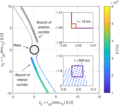
Figure 3: Capture set $\mathcal{C}_{-1}^{2}$ at $t_{0}=$ December 9, 2023 at 12:00:00 (UTC). Branches developing exterior BBCs are colored in gray. Regularity index [10] of ICs belonging to branches developing interior BCCs. Nondimensional coordinates on the orbital plane $i_{0}=\Omega_{0}=$0.2$\pi\,$\mathrm{rad}$$ defined in the Mars-centered RTN@$t_{0}$ frame. Mars is the gray circle with black surround. In the magnifications, details of chosen capture subsets.

To verify the applicability of PCE to the subcorridor synthesis, the influence of the subset dimensions on the expansion parameters (i. e., $m_{i}$ and $p$) is investigated. Firstly, the correlation between the quadrature nodes number $m_{i}$ and the side length $l$ is assessed. For this analysis, the polynomial basis order is kept constant to $p=6$. The range [5, 25] is assumed for $m_{i}$. The outcome is displayed in Fig. 4. The accuracy is evaluated at the beginning of the pre-capture trajectory (i. e., epoch $t_{f}=t_{0}-$400\text{\,}\mathrm{days}$$). For $5\leq m_{i}\leq 10$, the level curves show a ramp-like behavior. Intuitively, the accuracy increases with the density of quadrature nodes. For instance, consider a side length $l=$150\text{\,}\mathrm{km}$$, by progressively increasing $m_{i}$ from 5 to 10, it improves by three digits, both in position and velocity. However, for $m_{i}>10$, a plateau is reached. This is because theoretical results suggests that, for an increasing number of nodes, the estimation accuracy does not improve significantly once the estimation is exact. With exact estimation, it is intended the Gaussian quadrature exactness for polynomial of degree $p\leq(2m_{i}-1)$ [20]. On the other hand, the method seems to fail for $l=$300\text{\,}\mathrm{km}$$. The error in position is stuck in the order of $\mathrm{km}$ and accuracy stops improving with quadrature nodes number.

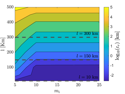
(a)

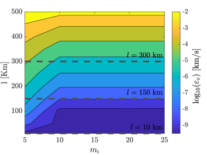
(b)

Figure 4: Approximation error at $t_{f}$ as a function of quadrature nodes number $m_{i}$ and square side length $l$. Polynomial basis order fixed to $p=6$. Specific subsets having constant $l$ highlighted with dashed horizontal lines.

Next, the correlation between the polynomial basis order $p$ and the side length $l$ is investigated. For this analysis, the quadrature nodes number is kept constant to $m_{i}=10$. Results are shown in Fig. 5. Remarkably, the method accuracy is greatly affected by the polynomial basis order. Indeed, the method accuracy improves by progressively increasing $p$. For $l=$100\text{\,}\mathrm{km}$$, the approximation errors decrease by one order of magnitude when $p$ increases from 6 to 10. Nevertheless, accuracy is lost when increasing indefinitely the polynomial basis order. As clearly visible on the right of plots in Fig. 5, increasing $p$ results in being a disadvantage for the method accuracy. This behavior may be justified considering that accuracy of Gaussian quadrature rule is exact for polynomials of degree $p\leq(2m_{i}-1)$ [20]. The latter translates into the necessity of rising the quadrature nodes density as $p$ increases. From Fig. 5, it is clear how for large $p$ values, the quadrature rule fails in estimating accurately the integral in Eq. (5), thereby growing the approximation error.

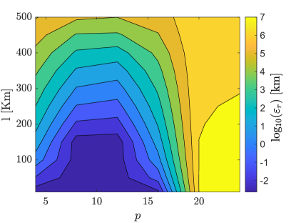
(a)

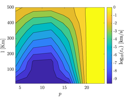
(b)

Figure 5: Approximation error at $t_{f}$ as a function of polynomial basis order $p$ and square side length $l$. Quadrature nodes number fixed to $m_{i}=10$.

4.2 Simulation parameters

The correlation between $m_{i}$ and $p$ is now investigated by fixing the square side length of the chosen capture subset to $l=$10\text{\,}\mathrm{km}$$. In this analysis, the quadrature nodes number $m_{i}$ and the polynomial basis function $p$ are let vary in ranges [3, 15] and [4, 12], respectively. The outcome is proposed in Fig. 6. As already noted, the method accuracy is almost unchanged for large quadrature nodes numbers. Furthermore, for $m_{i}<9$, accuracy is lost as the polynomial basis order $p$ increases. The latter confirms what was previously discussed in Section 4.1.

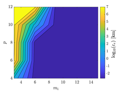
(a)

(b)

Figure 6: Approximation error at $t_{f}$ as a function of quadrature nodes number $m_{i}$ and polynomial basis order $p$. Square side length fixed to $l=$10\text{\,}\mathrm{km}$$.

4.3 Polynomial chaos coefficients distribution

The PCCs distribution for several $(m_{i},p)$ pairs, and with $l=$10\text{\,}\mathrm{km}$$ are shown in Fig. 7. In the plot, dots denote distributions $1\text{\,}\mathrm{day}$ before capture, while crosses the distributions $400\text{\,}\mathrm{days}$ before capture (corresponding to epoch $t_{f}$). Coefficients are normalized with respect to coefficient $c_{0}$. The higher the decay rate, the more accurate is the expansion result. This is because higher order terms become less relevant [20].

Results show that for the (10, 6) pair convergence is achieved at both epochs. Namely, at $t_{0}-$1\text{\,}\mathrm{day}$$ the distribution converges to within machine precision ($\sim\!10^{-15}$). Differently, the normalized coefficients converge at a lower pace to a higher asymptotic value ($\sim\!10^{-10})$ at $t_{f}$. This is consistent with results presented in [20], according to which the convergence value can be correlated to the digit precision in the state estimate. Indeed, numerical errors increase with the propagation time, leading to lower digit precision. Nonetheless, the digit precision is very high, both in nondimensional position and velocity, therefore results are satisfactory.

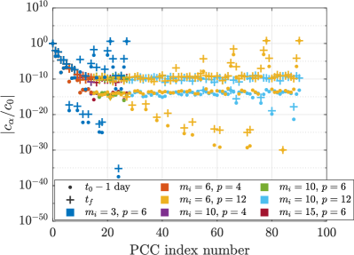
(a)

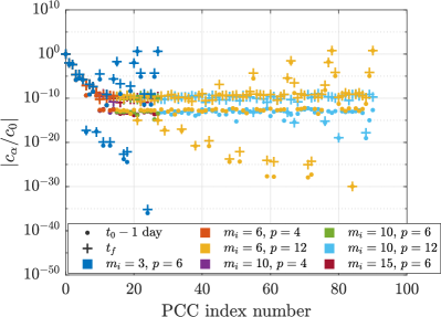
(b)

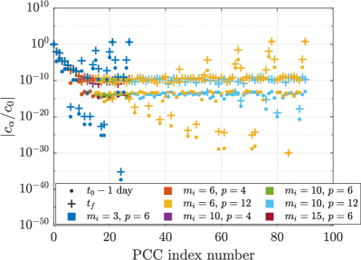
(c)

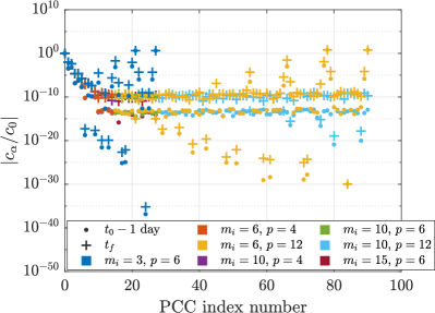
(d)

Figure 7: Normalized PCE coefficients distributions for 4 out of the 6 state variables. Dots and crosses indicate coefficients distribution $1\text{\,}$ and $400\text{\,}\mathrm{days}$ before capture, respectively. Note that $400\text{\,}\mathrm{days}$ before capture corresponds to the final backward propagation epoch $t_{f}$. Several $(m_{i},p)$ pairs shown.

Varying the quadrature nodes number, the expansion fails in achieving convergence for $m_{i}=3$. According to results in Fig. 6, $m_{i}>4$ is recommended. Contrarily, no significant variations are observed between the (10, 6) pair and the case with $m_{i}=15$. This is consistent with results in Figs. 4 and 6. Differently, by letting $p$ vary, convergence is assessed for (10, 4) and (10, 12) pairs. However, all high-order polynomials contribute marginally to the expansion accuracy for the (10, 12) pair. The latter representation is usually referred to as sparse [20]. Thus, only the most significant expansion coefficients are retained when $p=4$, thereby providing a good estimate of the system state. Finally, the top-right region of Fig. 6 is investigated. Convergence is achieved for the (6, 4) pair. Differently, the (6, 12) pair fails to converge since the quadrature rule is unsuccessful in accurately estimating the PCCs for $p>(2m_{i}-1)$ [20].

4.4 Validation

The PCE technique is validated against MC analysis. In the following, the convergence analysis focuses on a specific case study, which develops the corridor upon the same capture subset with $l=$10\text{\,}\mathrm{km}$$ described in Section 4.1. The selected simulation parameters are $m_{i}=10$ and $p=6$.

The convergence analysis is evaluated at fixed time epoch. Therefore, the epoch is suitably selected to assess the PCE validity in approximating the pre-capture trajectory. To this aim, the PCE and MC approaches are compared considering their evolution in time. Namely, the PCE estimated mean is compared with the mean estimate computed from $10^{2}$ samples. Samples are drawn with the Latin hypercube sampling (LHS) technique. In Fig. 8, the approximation error is evaluated as $\bm{e}(t)=|\bm{c}_{0}(t)-\bm{\mu}(t)|$, where $\bm{c}_{0}(t)$ is the first PCC, being the mean according to the PCE, and $\bm{\mu}(t)$ is the mean value retrieved with the MC analysis. From results, it is observed that the error increases with the propagation time (from $t_{0}$ to $t_{f}=$-400\text{\,}\mathrm{days}$$). It comes naturally to assess the method convergence at the final epoch $t_{f}$, which is associated with the largest approximation error.

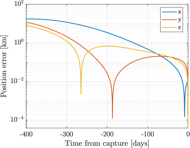
(a)

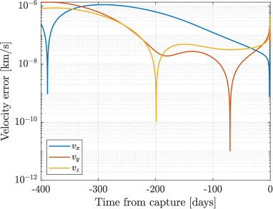
(b)

Figure 8: Method accuracy in estimating the mean. Evolution of first PCC compared to estimated mean drawn from capture subset with LHS technique and computed from $10^{2}$ samples.

The convergence is evaluated on the mean and standard deviation. Fig. 9 compares the results for the MC simulation and the PCE technique as a function of the samples $n$. Convergence errors are computed as

$$\varepsilon_{\mu_{r}}=\max_{i=x,y,z}\left|\dfrac{\mu^{\mathrm{MC}}_{i}(t_{f})-\mu^{\mathrm{PCE}}_{i}(t_{f})}{\mu^{\mathrm{PCE}}_{i}(t_{f})}\right|,\qquad\ \varepsilon_{\mu_{v}}=\max_{i=v_{x},v_{y},v_{z}}\left|\dfrac{\mu^{\mathrm{MC}}_{i}(t_{f})-\mu^{\mathrm{PCE}}_{i}(t_{f})}{\mu^{\mathrm{PCE}}_{i}(t_{f})}\right|,$$ (6)

$$\varepsilon_{\sigma_{r}}=\max_{i=x,y,z}\left|\dfrac{\sigma^{\mathrm{MC}}_{i}(t_{f})-\sigma^{\mathrm{PCE}}_{i}(t_{f})}{\sigma^{\mathrm{PCE}}_{i}(t_{f})}\right|,\qquad\ \varepsilon_{\sigma_{v}}=\max_{i=v_{x},v_{y},v_{z}}\left|\dfrac{\sigma^{\mathrm{MC}}_{i}(t_{f})-\sigma^{\mathrm{PCE}}_{i}(t_{f})}{\sigma^{\mathrm{PCE}}_{i}(t_{f})}\right|.$$ (7)

Referring to Fig. 9, the mean and standard deviation convergence errors for $n=10^{3}$ are $\varepsilon_{\mu_{r}}=$5.682\text{\times}{10}^{-8}$$, $\varepsilon_{\mu_{v}}=$2.924\text{\times}{10}^{-12}$$, $\varepsilon_{\sigma_{r}}=$4.943\text{\times}{10}^{-5}$$, and $\varepsilon_{\sigma_{v}}=$5.4235\text{\times}{10}^{-7}$$. Eventually, the MC analysis converges to the reference solution with a large degree of accuracy. Consistently with theoretical results predicted in the literature, the standard deviation converges at a lower rate with respect to the mean [40]. Therefore, the PCE technique is validated against the MC approach for the problem at hand. Remarkably, the MC approach with LHS requires the propagation of $10^{3}$ samples, whereas only $m_{i}^{d}=10^{2}$ propagations are required by the PCE method when applied to this case study.

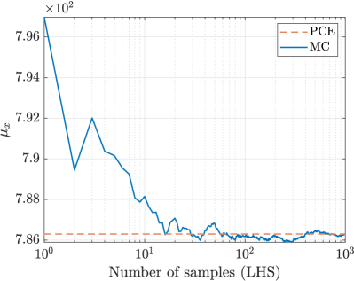
(a)

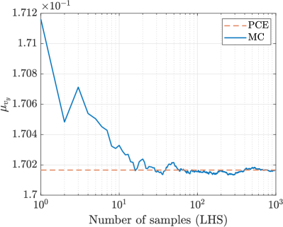
(b)

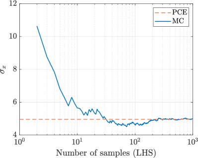
(c)

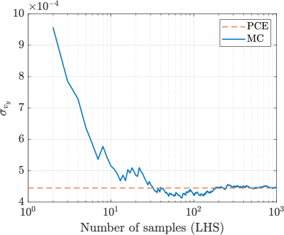
(d)

Figure 9: Estimated mean and standard deviation at $t_{f}=t_{0}-$400\text{\,}\mathrm{days}$$ for 2 out of the 6 state variables. Results from MC simulation (solid blu line) and PCE (dashed red line) as a function of samples number. Nondimensional quantities (see Table 2) in the Mars-centered J2000 frame.

5 Conclusion

In this paper, a procedure to accurately and inexpensively synthesize ballistic capture corridors exploiting the polynomial chaos expansion technique is discussed and validated against Monte Carlo simulations. Results prove the convergence of the method, assess the feasibility of ballistic capture corridor numerical synthesis, and highlight its convenience in terms of computational efficiency. Remarkably, as the capture subset dimension increases, the method accuracy is preserved by properly tuning the quadrature nodes number and the polynomial basis order. For constant polynomial basis order, the method accuracy improves as the number of quadrature nodes increases up to the point a plateau is reached. Denser quadrature nodes imply higher computational costs, reducing the computational efficiency and making the ballistic capture corridor construction more expensive. On the other hand, for fixed quadrature nodes number, the method accuracy does not improve by increasing the polynomial basis order. Indeed, the method accuracy decreases because the quadrature nodes are insufficient, thereby poorly estimating high-order polynomials. Overall, results show that a convenient combination of quadrature nodes number and polynomial basis order improves the accuracy of the method at limited computational costs.

Funding Sources

The authors would like to acknowledge the European Research Council (ERC) since part of this work has received funding from the ERC under the European Union’s Horizon 2020 research and innovation programme (Grant Agreement No. 864697).

References

- Poghosyan and Golkar [2017] Poghosyan, A., and Golkar, A., “CubeSat evolution: Analyzing CubeSat capabilities for conducting science missions,” Progress in Aerospace Sciences, Vol. 88, 2017, pp. 59–83. 10.1016/j.paerosci.2016.11.002.
- Bandyopadhyay et al. [2016] Bandyopadhyay, S., Foust, R., Subramanian, G. P., Chung, S.-J., and Hadaegh, F. Y., “Review of formation flying and constellation missions using nanosatellites,” Journal of Spacecraft and Rockets, Vol. 53, No. 3, 2016, pp. 567–578. 10.2514/1.a33291.
- Kalita et al. [2017] Kalita, H., Asphaug, E., Schwartz, S., and Thangavelautham, J., “Network of nano-landers for in-situ characterization of asteroid impact studies,” 68th International Astronautical Congress, Adelaide, Australia, 2017. IAC-17-D3.3.2.
- Hein et al. [2018] Hein, A. M., Saidani, M., and Tollu, H., “Exploring potential environmental benefits of asteroid mining,” 69th International Astronautical Congress, Bremen, Germany, 2018. IAC-18,D4,5,11,x47396.
- Di Domenico et al. [2022] Di Domenico, G., Andreis, E., Morelli, A. C., Merisio, G., Franzese, V., Giordano, C., Morselli, A., Panicucci, P., Ferrari, F., and Topputo, F., “The ERC-funded EXTREMA project: Achieving self-driving interplanetary CubeSats,” Modeling and Optimization in Space Engineering –- New Concepts and Approaches, Springer, Cham, Switzerland, 2022, pp. 167–199. 10.1007/978-3-031-24812-2_6.
- Turan et al. [2022] Turan, E., Speretta, S., and Gill, E., “Autonomous navigation for deep space small satellites: Scientific and technological advances,” Acta Astronautica, Vol. 193, 2022, pp. 56–74. 10.1016/j.actaastro.2021.12.030.
- Andreis et al. [2022] Andreis, E., Franzese, V., and Topputo, F., “Onboard orbit determination for deep-space CubeSats,” Journal of Guidance, Control, and Dynamics, Vol. 45, No. 8, 2022, pp. 1466–1480. 10.2514/1.G006294.
- Hyeraci and Topputo [2010] Hyeraci, N., and Topputo, F., “Method to design ballistic capture in the elliptic restricted three-body problem,” Journal of Guidance, Control, and Dynamics, Vol. 33, No. 6, 2010, pp. 1814–1823. 10.2514/1.49263.
- Luo et al. [2014] Luo, Z.-F., Topputo, F., Bernelli Zazzera, F., and Tang, G. J., “Constructing ballistic capture orbits in the real Solar System model,” Celestial Mechanics and Dynamical Astronomy, Vol. 120, No. 4, 2014, pp. 433–450. 10.1007/s10569-014-9580-5.
- Dei Tos et al. [2018] Dei Tos, D. A., Russell, R. P., and Topputo, F., “Survey of Mars ballistic capture trajectories using periodic orbits as generating mechanisms,” Journal of Guidance, Control, and Dynamics, Vol. 41, No. 6, 2018, pp. 1227–1242. 10.2514/1.G003158.
- Topputo and Belbruno [2015] Topputo, F., and Belbruno, E., “Earth–Mars transfers with ballistic capture,” Celestial Mechanics and Dynamical Astronomy, Vol. 121, No. 4, 2015, pp. 329–346. 10.1007/s10569-015-9605-8.
- Belbruno and Miller [1993] Belbruno, E., and Miller, J., “Sun-perturbed Earth-to-Moon transfers with ballistic capture,” Journal of Guidance, Control, and Dynamics, Vol. 16, No. 4, 1993, pp. 770–775. 10.2514/3.21079.
- Belbruno and Carrico [2000] Belbruno, E., and Carrico, J., “Calculation of weak stability boundary ballistic lunar transfer trajectories,” Astrodynamics Specialist Conference, Denver, CO, 2000. 10.2514/6.2000-4142, aIAA 2000-4142.
- Quinci et al. [2023] Quinci, A., Merisio, G., and Topputo, F., “Qualitative study of ballistic capture at Mars via Lagrangian descriptors,” Communications in Nonlinear Science and Numerical Simulation, Vol. 123, 2023, p. 107285. 10.1016/j.cnsns.2023.107285.
- Merisio [2023] Merisio, G., “Engineering ballistic capture for autonomous interplanetary spacecraft with limited onboard resources,” Ph.D. thesis, Politecnico di Milano, Milan, Italy, 2023. URL https://hdl.handle.net/10589/196152.
- Morelli et al. [2022] Morelli, A. C., Merisio, G., Hofmann, C., and Topputo, F., “A Convex Guidance Approach to Target Ballistic Capture Corridors at Mars,” 44th AAS Guidance, Navigation and Control Conference, Breckenridge, CO, 2022. AAS 22-083.
- Aguiar and Topputo [2018] Aguiar, G., and Topputo, F., “A Technique for Designing Earth–Mars Low-Thrust Transfers Culminating in Ballistic Capture,” 7th International Conference on Astrodynamics Tools and Techniques (ICATT), Oberpfaffenhofen, Germany, 2018.
- Luo and Topputo [2015] Luo, Z.-F., and Topputo, F., “Analysis of ballistic capture in Sun–planet models,” Advances in Space Research, Vol. 56, No. 6, 2015, pp. 1030–1041. 10.1016/j.asr.2015.05.042.
- Giordano [2021] Giordano, C., “Analysis, Design, and Optimization of Robust Trajectories for Limited-Capability Small Satellites,” Ph.D. thesis, Politecnico di Milano, Milan, Italy, 2021. URL http://hdl.handle.net/10589/177695.
- Jones et al. [2013] Jones, B. A., Doostan, A., and Born, G. H., “Nonlinear propagation of orbit uncertainty using non-intrusive polynomial chaos,” Journal of Guidance, Control, and Dynamics, Vol. 36, No. 2, 2013, pp. 430–444. 10.2514/1.57599.
- Pugliatti et al. [2023] Pugliatti, M., Giordano, C., and Topputo, F., “The image processing of Milani: challenges after DART impact,” 12th International Conference on Guidance, Navigation and Control Systems (GNC), Sopot, Poland, 2023.
- Caleb et al. [2022] Caleb, T., Merisio, G., Di Lizia, P., and Topputo, F., “Stable sets mapping with Taylor differential algebra with application to ballistic capture orbits around Mars,” Celestial Mechanics and Dynamical Astronomy, Vol. 134, No. 5, 2022, pp. 1–22. 10.1007/s10569-022-10090-8.
- Park et al. [2021] Park, R. S., Folkner, W. M., Williams, J. G., and Boggs, D. H., “The JPL Planetary and Lunar Ephemerides DE440 and DE441,” The Astronomical Journal, Vol. 161, No. 3, 2021, p. 105. 10.3847/1538-3881/abd414.
- Huang et al. [1990] Huang, C., Ries, J. C., Tapley, B. D., and Watkins, M. M., “Relativistic effects for near-Earth satellite orbit determination,” Celestial Mechanics and Dynamical Astronomy, Vol. 48, No. 2, 1990, pp. 167–185. 10.1007/BF00049512.
- Topputo et al. [2021] Topputo, F., Wang, Y., Giordano, C., Franzese, V., Goldberg, H., Perez-Lissi, F., and Walker, R., “Envelop of reachable asteroids by M-ARGO CubeSat,” Advances in Space Research, Vol. 67, No. 12, 2021, pp. 4193–4221. 10.1016/j.asr.2021.02.031.
- Dei Tos and Topputo [2019] Dei Tos, D. A., and Topputo, F., “High-fidelity trajectory optimization with application to saddle-point transfers,” Journal of Guidance, Control, and Dynamics, Vol. 42, No. 6, 2019, pp. 1343–1352. 10.2514/1.G003838.
- Gottlieb [1993] Gottlieb, R. G., “Fast gravity, gravity partials, normalized gravity, gravity gradient torque and magnetic field: Derivation, code and data,” Tech. rep., 1993. 188243, prepared for Lyndon B. Johnson Space Center under contract NAS9-17885.
- Acton [1996] Acton, C., “Ancillary data services of NASA’s navigation and ancillary information facility,” Planetary and Space Science, Vol. 44, No. 1, 1996, pp. 65–70. 10.1016/0032-0633(95)00107-7.
- Acton et al. [2018] Acton, C., Bachman, N., Semenov, B., and Wright, E., “A look towards the future in the handling of space science mission geometry,” Planetary and Space Science, Vol. 150, 2018, pp. 9–12. 10.1016/j.pss.2017.02.013.
- Topputo et al. [2018] Topputo, F., Dei Tos, D. A., Mani, K. V., Ceccherini, S., Giordano, C., Franzese, V., and Wang, Y., “Trajectory design in high-fidelity models,” 7th International Conference on Astrodynamics Tools and Techniques (ICATT), Oberpfaffenhofen, Germany, 2018, pp. 1–9.
- Montenbruck and Gill [2000] Montenbruck, O., and Gill, E., Satellite Orbits Models, Methods and Applications, Springer, Heidelberg, Germany, 2000. 10.1007/978-3-642-58351-3, pages 117–156.
- Prince and Dormand [1981] Prince, P. J., and Dormand, J. R., “High order embedded Runge–Kutta formulae,” Journal of Computational and Applied Mathematics, Vol. 7, No. 1, 1981, pp. 67–75. 10.1016/0771-050x(81)90010-3.
- Luo and Topputo [2021] Luo, Z.-F., and Topputo, F., “Mars orbit insertion via ballistic capture and aerobraking,” Astrodynamics, Vol. 5, No. 2, 2021, pp. 167–181. 10.1007/s42064-020-0095-4.
- Giordano and Topputo [2022] Giordano, C., and Topputo, F., “Aeroballistic Capture at Mars: Modeling, Optimization, and Assessment,” Journal of Spacecraft and Rockets, 2022, pp. 1–15. 10.2514/1.A35176.
- Merisio and Topputo [2021] Merisio, G., and Topputo, F., “Characterization of ballistic capture corridors aiming at autonomous ballistic capture at Mars,” 2021 AAS/AIAA Astrodynamics Specialist Conference, Big Sky, Virtual, 2021. AAS 21-677.
- Luo and Topputo [2017] Luo, Z.-F., and Topputo, F., “Capability of satellite-aided ballistic capture,” Communications in Nonlinear Science and Numerical Simulation, Vol. 48, 2017, pp. 211–223. 10.1016/j.cnsns.2016.12.021.
- Xiu and Karniadakis [2002] Xiu, D., and Karniadakis, G. E., “The Wiener–Askey Polynomial Chaos for Stochastic Differential Equations,” SIAM Journal on Scientific Computing, Vol. 24, No. 2, 2002, pp. 619–644. 10.1137/S1064827501387826.
- Luo [2020] Luo, Z.-F., “The role of the mass ratio in ballistic capture,” Monthly Notices of the Royal Astronomical Society, Vol. 498, No. 1, 2020, p. 1515–1529. 10.1093/mnras/staa2366.
- Merisio and Topputo [2022] Merisio, G., and Topputo, F., “An algorithm to engineer autonomous ballistic capture at Mars,” 73rd International Astronautical Congress, Paris, France, 2022. IAC-22,C1,9,10,x73057.
- Xiu [2010] Xiu, D., Numerical methods for stochastic computations: a spectral method approach, Princeton University Press, Princeton, NJ, 2010. 10.1515/9781400835348, Chap. 1, 4.