Cold diffuse interstellar medium of Magellanic Clouds: I. HD molecule and cosmic-ray ionization rate

Abstract

HD molecule is one the most abundant molecules in the Universe and due to its sensibility to the conditions in the medium, it can be used to constrain physical parameters in the medium where HD resides. Lately we have shown that HD abundance can be enhanced in the low metallicity medium. Large and Small Magellanic Clouds give us an opportunity to study low metallicity galaxies in details towards different sightlines due to their proximity to our Galaxy. We revisited FUSE space telescope archival spectra towards bright stars in Magellanic Clouds to search for HD molecules, associated with the medium of these galaxies. We reanalysed H₂ absorption lines and constrained HD column density at the positions of H₂ components. We detected HD towards 24 sightlines (including 19 new detections). We try to measure cosmic ray ionization rate for several systems using measured $N({\rm HD})/N({\rm H_{2}})$, and in most cases get loose constraints due to insufficient quality of the FUSE spectra.

1 Introduction

The physical state of interstellar medium (ISM) is in the close relationship with the galaxy evolution, since it determines the star-formation, a key process of galaxy formation. On the other hand, stars influence environment around, by enrichment of the ISM with metals and dust, supply of the ultraviolet (UV) radiation and cosmic rays, energy and momentum injection etc. These change rates of reactions in the ISM, and hence impact on the abundances and level populations of the species. Therefore spectroscopic analysis of latter gives us opportunity to constrain the physical conditions in the observed systems, using comparison with the models.

Star-formation occurs in the molecular gas, which predominantly consists of H₂, which is hard to observe in the emission in cold ISM. Hence usually other tracers of H₂ are used, out of which CO is most abundant ($n({\rm CO})/n({\rm H_{2}})\lesssim 10^{-4}$, where $n({\rm X})$ – is a number density of species) and exhaustively studied. However, H₂ can be easily observed in absorption using UV resonant transition (see recent note by Shull, 2022). Unlike CO, H₂ in UV band predominantly probes diffuse molecular and translucent medium, due to saturation effects and associated extinction. However, such gas is certainly in intimate connection with the dense molecular gas, either providing its supply, or being the remnants of the intermittent molecular clouds.

Similar to H₂, HD – an isotopologue of H₂ with abundance $n({\rm HD})/n({\rm H_{2}})\sim 10^{-5}$, can be detected in the absorption using resonant transitions in UV band in our Galaxy (e.g. Snow et al., 2008) and in optical band at high redshifts (e.g. Varshalovich et al., 2001; Tumlinson et al., 2010; Ivanchik et al., 2015; Noterdaeme et al., 2017; Kosenko et al., 2021, and references therein). The importance of HD for ISM studies has been discussed starting from its detection (e.g. Black & Dalgarno, 1973; Hartquist et al., 1978), since HD provides an opportunity to constrain physical conditions in the medium, associated with absorption systems. Indeed, at the moderate presence of H₂, HD molecules form through a fast ion-molecular reaction:

$${\rm H_{2}+D^{+}\longrightarrow HD+H^{+}},$$ (1)

and destructed by photodissociation. This makes relative abundance of HD/H₂ sensitive to the main physical conditions in the medium, namely, number density, $n$, UV field intensity, $\chi$, abundance of metals (and their depletion), and cosmic ray ionisation rate (CRIR), $\zeta$. Regarding the latter, cosmic rays determine H⁺ formation, which defines the ionized deuterium, D⁺ abundance through charge exchange reaction, and therefore CRIR directly affects HD production rate.

Using a balance equation between HD formation (adding formation on the dust grains, which may be sufficient on the edge of the cloud, where there H₂ abundance is small $n({\rm H_{2}})/n_{\rm tot}\lesssim 10^{-4}$, and rate of reaction 1 is negligible) and destruction by UV radiation (taking into account self-shielding) we have recently obtained a simple semi-analytical formalism for dependence of HD/H₂ abundance on the aforementioned parameters (Balashev & Kosenko, 2020) which allows us to constrain the physical conditions in the medium. One of the most important results of this recent study is that measured HD/H₂ ratios allow us to get constraints on CRIR in diffuse molecular medium of high-redshift galaxies., therefore we have applied our method to a sample of all known HD/H₂ absorption systems at high redshifts (Kosenko et al., 2021). More intriguing, we also showed that HD abundance is really enhanced in the low-metallicity medium probed by high-z Damped Lyman alpha (DLA) systems in comparison with high metallicities (Balashev & Kosenko, 2020; Kosenko et al., 2021), as a consequence of enhanced ionization fractions. This behaviour of HD at low metallicity can be tested on the local dwarf galaxies, out of which the Large and Small Magellanic Clouds (LMC and SMC, respectively), seem to be the most appropriate, since they provide individually resolved stars due to their proximity to the Milky Way. Additionally, studies of diffuse gas with HD/H₂ provide us with valuable constraints on the physical conditions, which are known to differ much from our Galaxy.

LMC and SMC are the closest dwarf galaxies to the Milky Way. Distance to LMC is about 50 kpc (Pietrzyński et al., 2019) and it is a spiral galaxy with bar and bright dominant north spiral arm and a weak south arm. Average metallicity in the LMC is about 0.5 relative to solar (Russell & Dopita, 1992). Most of the star-formation activity occurs in the bar and in the dominant arm, e.g. one of the most studied star-forming complex, 30 Dor, is located in the northeast of the bar. Distance to the SMC is about 62 kpc (Graczyk et al., 2020) and it is an irregular galaxy and can be divided to a bar (most dense, turbulent and UV exposed region of the SMC) and more quiescent and less dense wing on the east side. Metallicity of the SMC is about 0.2 relative to solar (Russell & Dopita, 1992) and it is comparable with the average metallicity in the high redshift DLAs. From the east of the wing of SMC to the west side of the LMC there has been discovered Magellanic Bridge, a stream of neutral hydrogen with several stars (Hindman et al., 1963), which, as believed, was created due to the interaction between LMC and SMC about 200 Myr ago. Abundances in the Magellanic Bridge differ significantly from the abundances in both LMC and SMC and may be lower even then in the SMC (e.g. Lehner et al., 2008; Dufton et al., 2008; Lee et al., 2005; Ramachandran et al., 2021).

Proximity of Magellanic Clouds to our Galaxy gives us a perfect opportunity to study low metallicity galaxies in detail and to observe systems along different lines of sight within one galaxy. As we mentioned above, H₂ and HD are available in local Universe only using UV space telescopes. Fortunately, Far Ultraviolet Spectroscopic Explorer (FUSE) have been successfully used to study cold diffuse medium with HD and H₂ in the Milky Way (Snow et al., 2008; Shull et al., 2021) and with H₂ in Magellanic Clouds (Welty et al., 2012).

The main purpose of the work is to search for HD molecules in Magellanic Clouds using archival data obtained by FUSE telescope, to constrain HD/H₂ relative abundances in this satellite galaxies. Using measured HD and H₂ column density we tried to constrain cosmic ray ionization rates in the analysed systems. To our knowledge there was no attempt made to estimate CRIR in the Magellanic Clouds using the abundance matching. However, some constraints of cosmic-ray flux in LMC and SMC were obtained using gamma-ray radiation, that found average cosmic-ray density in both LMC and SMC lower then in Solar neighborhood (see e.g. Ackermann et al., 2016; Lopez et al., 2018). Nevertheless, one should bear in mind, that only cosmic rays with energies $>280$ MeV contribute into gamma-ray flux due to pion decay, while ISM is ionized mostly by low-energy cosmic rays $\lesssim 100$ MeV. Also low-energy cosmic rays may be trapped in the region where they were accelerated and their flux (and therefore CRIR) depends on the distance to the star-forming regions and supernova remnants. This paper is accompanied by another one (Kosenko in prep.), which is focused on the constraints on the number density and UV flux in LMC and SMC using the population of the rotational levels of H₂ (measured and presented in this paper) and C i fine-structure levels.

The paper is organized as follows: in Section 2 we describe a sample of data which was used in the work, in Section 3 we provide a description of the method to analyse observations, including line profile fitting. The results of data analysis, including new HD detections, are presented in Section 4. In the Section 5 we the describe constraint on the cosmic ray ionization rate obtained from measured HD/H₂ ratio. Section 6 we discuss how high resolution observations may improve obtained constraints, before summarizing the obtained results in Section 7.

2 Data

HD and H₂ absorption lines fall into UV part of electromagnetic spectrum $(\lambda_{\rm H_{2}}\rm\lesssim 110\,nm)$, therefore observations of these molecules are limited due to the atmospheric absorption. The progress of H₂ observations in the Milky Way and the local Universe was certainly attributed to availability of the space UV telescopes. The best resolution and quality observations were performed by Far Ultraviolet Spectroscopic Explorer (FUSE, Moos et al. 2000; Sahnow et al. 2000), which covers 907-1187 Å  and have nominal spectral resolution $R\sim 20000$.

Blair et al. 2009 collected all of the FUSE observations in Magellanic Clouds and reprocessed them with the final calibration pipeline (CalFUSE 3.2) to get uniform data (FUSE Magellanic Clouds Legacy Project). Using these data Welty et al. 2012 have found H₂ in 80 sightlines in LMC and in 65 sightlines in SMC. We selected those systems where $\log N_{\rm H_{2}}\gtrsim 18$, since the quality of FUSE spectra does not allow detection of $\log N_{\rm HD}\lesssim 13$ (typically measured relative abundance $N({\rm HD})/N({\rm H_{2}})\lesssim 10^{-5}$). This cut the sample to 48 sightlines in the LMC and 46 sightlines in the SMC.

The fully reduced spectra of the systems towards bright stars in LMC are available in the FUSE Magellanic Clouds Legacy Project (Blair et al., 2009). Typical observation of a star consists of the several exposures, obtained in different FUSE channels. We used spectra from 1A LiF channel, as it covers most of HD and H₂ absorption lines and has relatively high sensitivity (Dixon et al., 2007). Unfortunately, most of FUSE spectra suffer from inappropriate calibration issues, so we made an attempt to improve the quality of calibration. First, we find a zero-order spectrum, which is obtained by coadding of exposures, using the constant velocity shifts, that was found from the procedure of cross-correlation (Simkin, 1974; Tonry & Davis, 1979). From the zero-order spectrum we obtained rough estimates on H₂ column densities, Doppler parameters and redshifts. Then, using H₂ synthetic spectrum, constructed from these estimates, as a template, we obtained a wavelength dependent shifts for each exposure. We took only narrow, unblended lines and cross-correlated them with the template. The wavelength dependency of the estimated shifts was interpolated with piece-wise linear function, that was finally applied to correct the exposures, during coadding.

3 Analysis

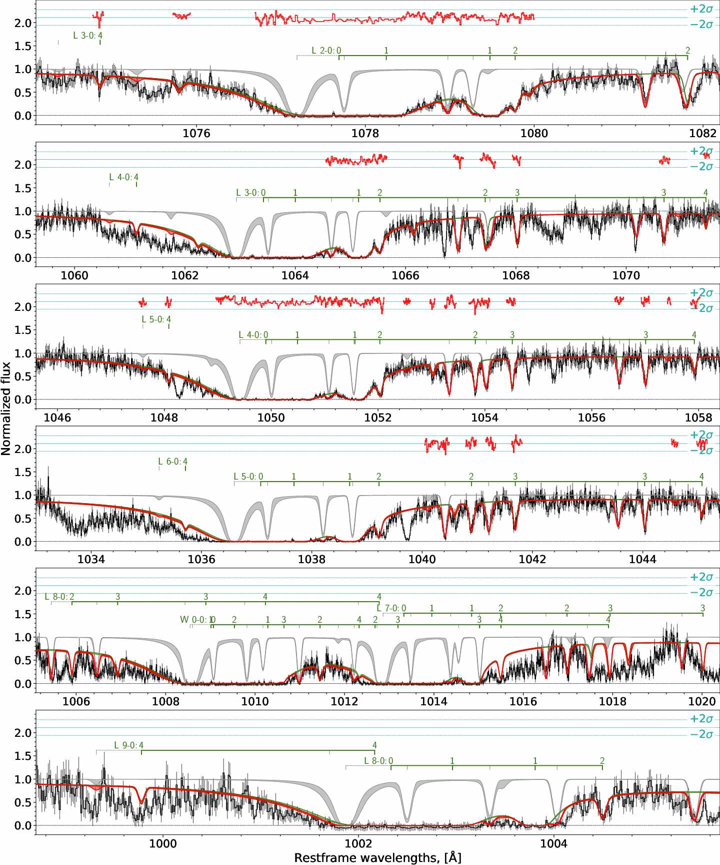
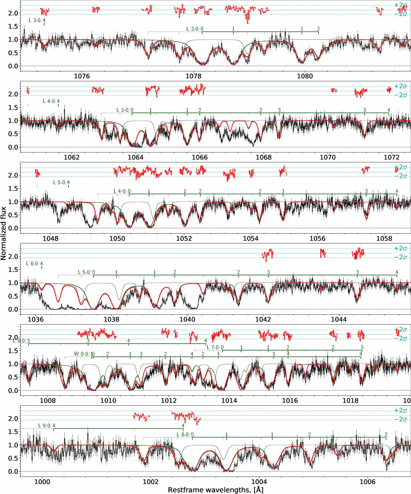
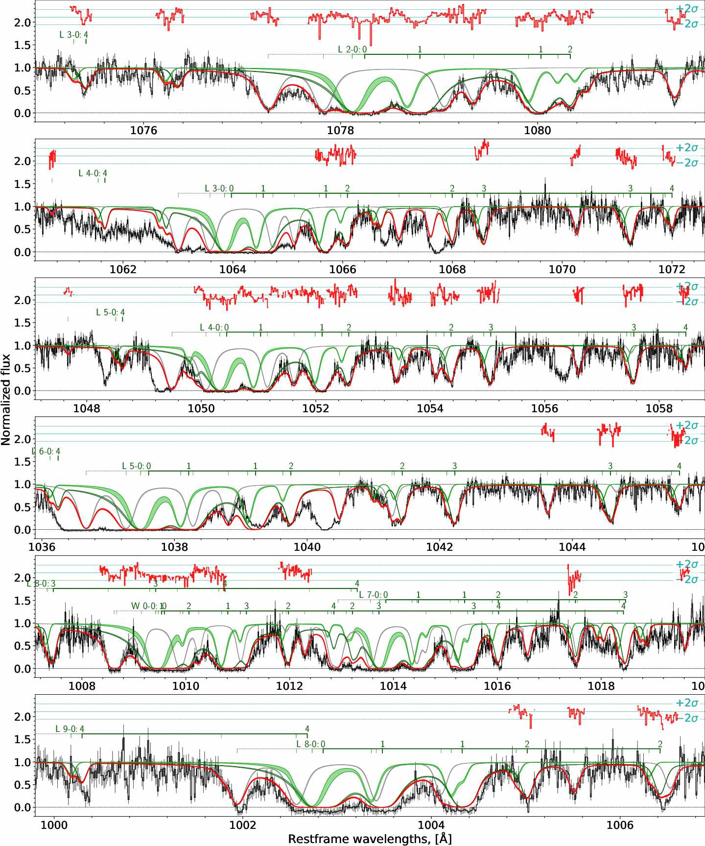
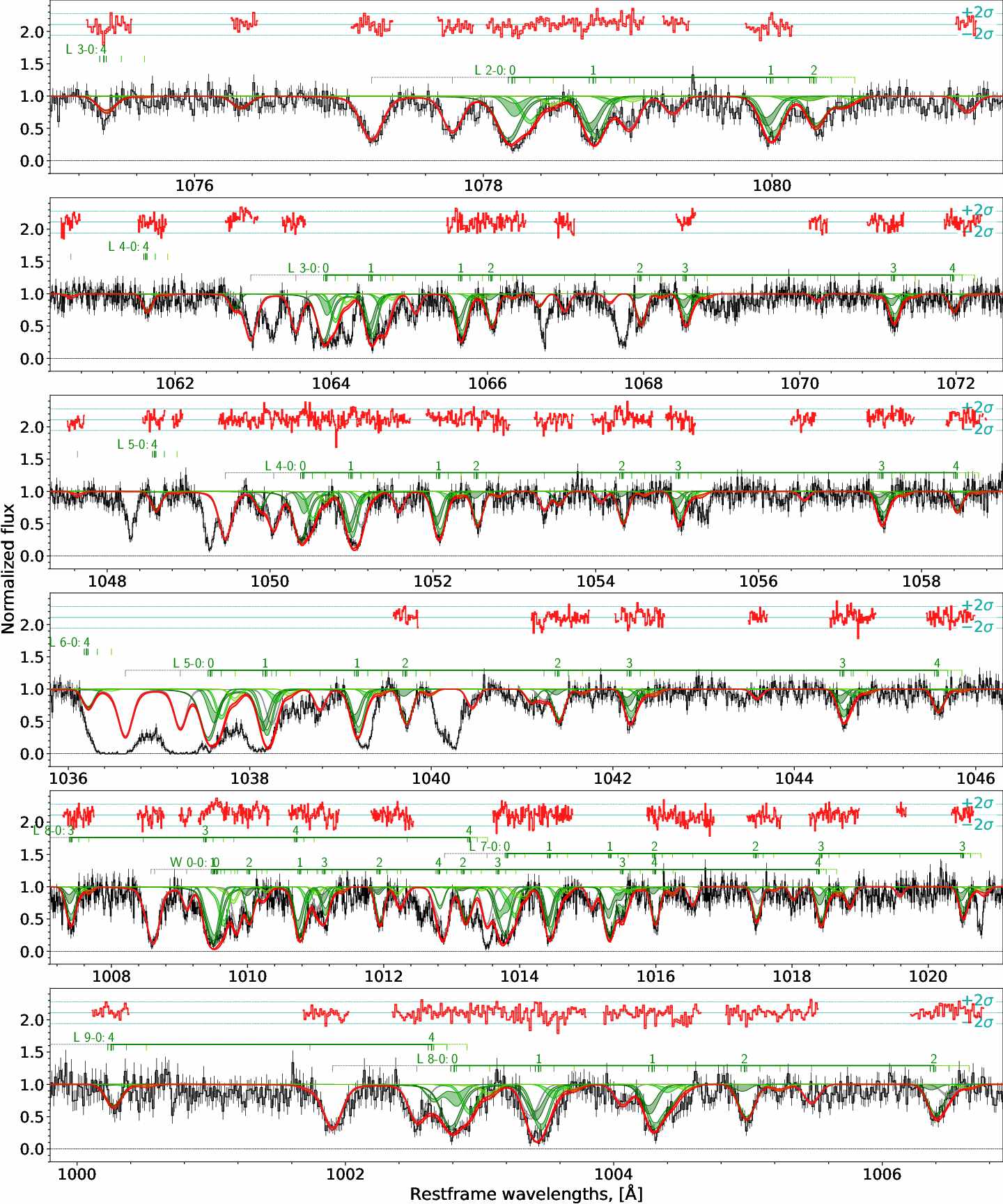
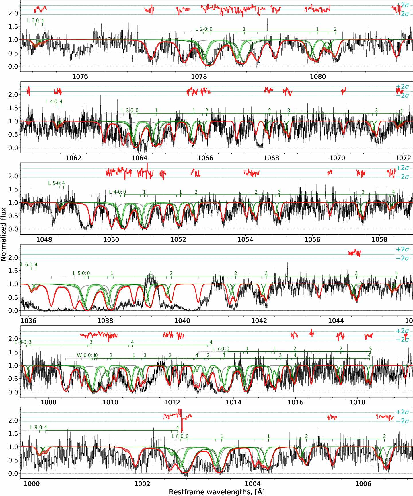
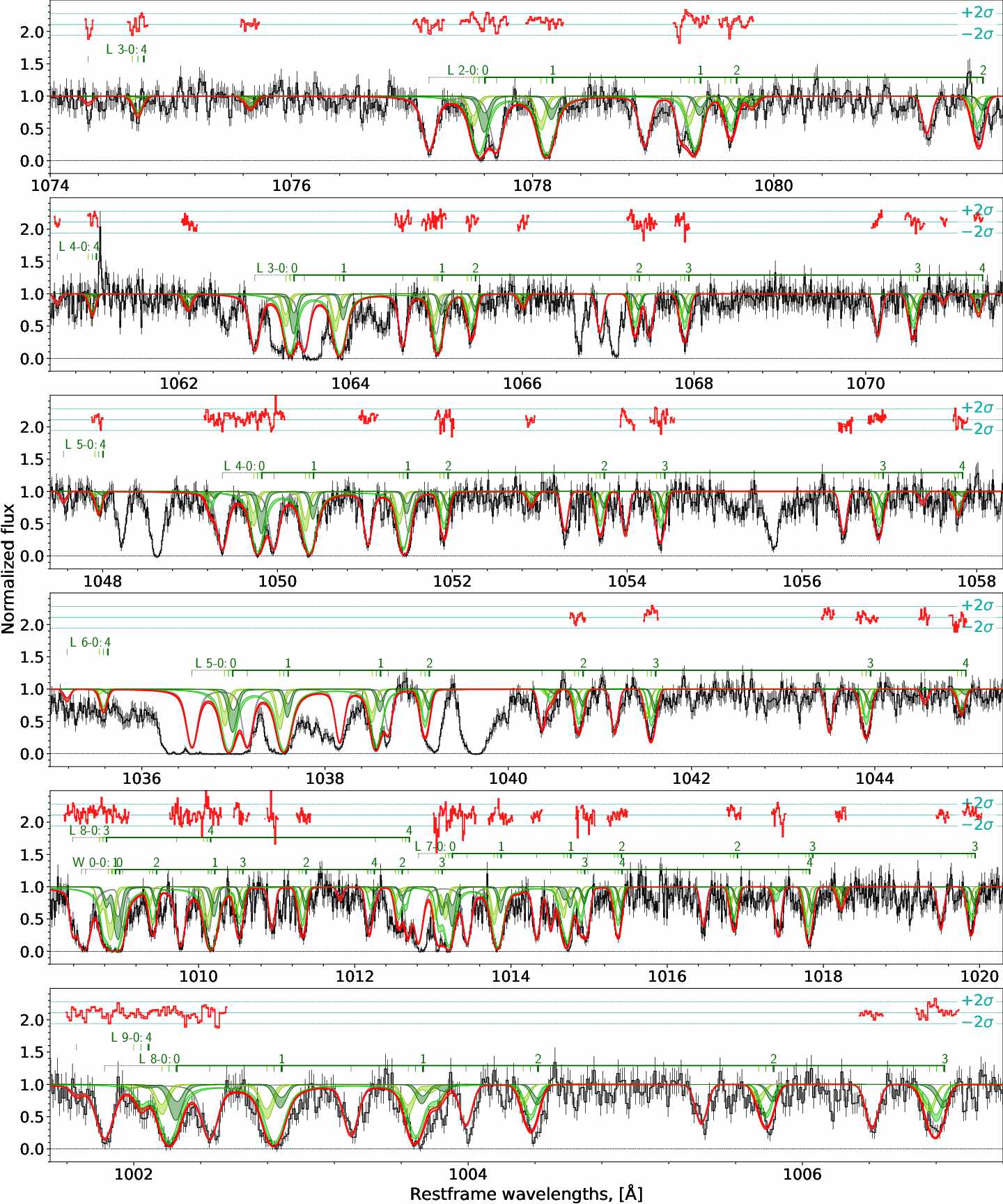
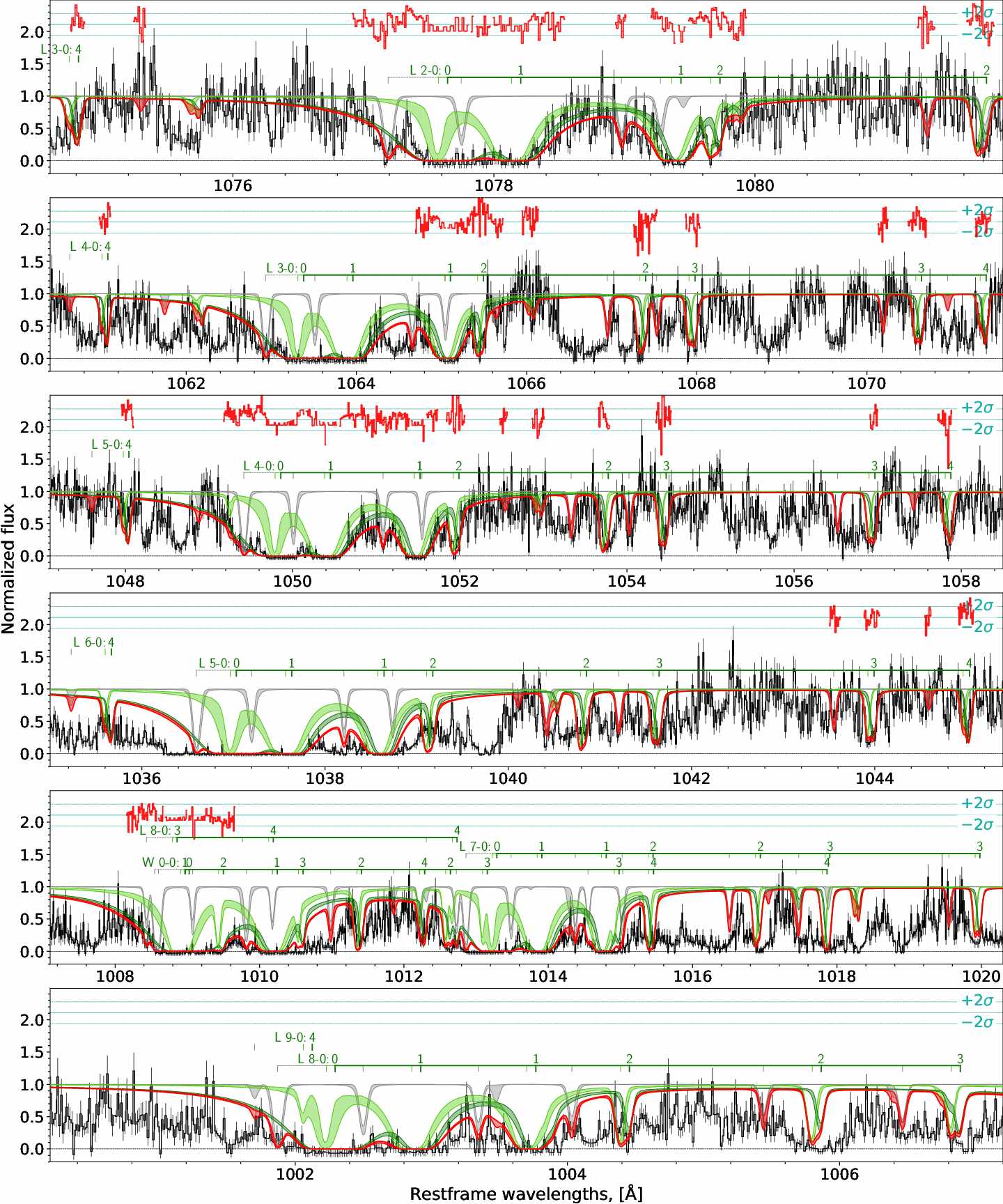
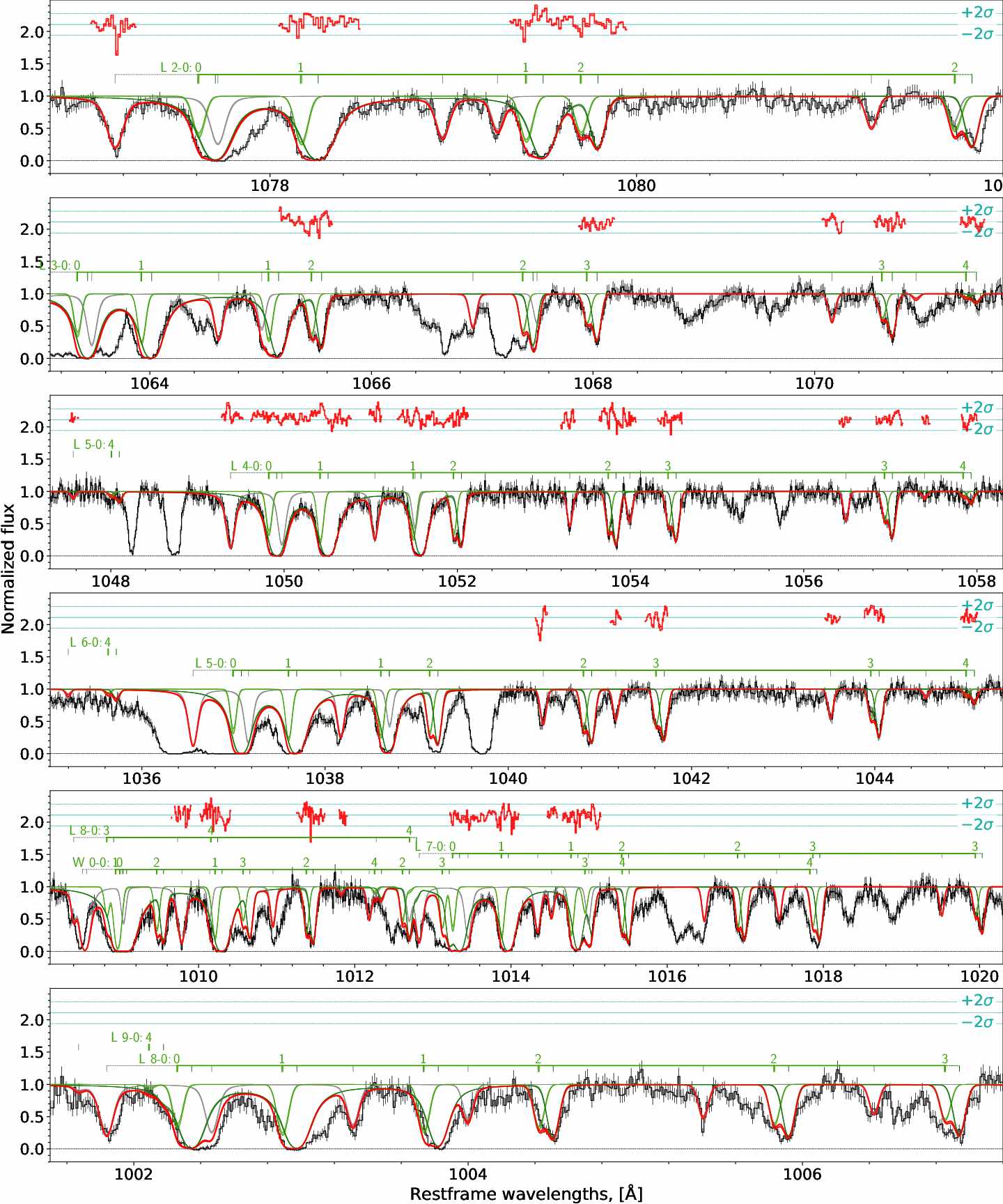
We model line profiles with standard multicomponent Voigt profile fitting using Monte Carlo Markov Chain (MCMC) sampler to obtain posterior distribution function of the absorption system parameters: column densities ($N$, measured throughout the paper in cm^-2), Doppler parameters, ($b$) and redshifts ($z$). The continuum was independently constructed for each considered fit (H₂, HD, etc) by B-splain interpolation of the neighboring regions of absorption lines, clear from the evident absorptions. We note that in the case of the saturated H₂ lines, which show Lorentzian wings this is a bit ambiguous task, therefore we iteratively adjusted continuum in the case of outlying lines. To construct the synthetic spectrum we used HD and H₂ transition lines and molecular data, collected by Ubachs et al. 2019.

To estimate parameters and its uncertainties we used maximum aposteriori probability and $68.3\%$ credible intervals, respectively. We judge between detection and non detection of HD based on the constrained column density posterior probability function. For the cases where it shows a solitary peak we reported a measurement, while if there is a significant amount of the posterior near the lower end of column density range (taken to be $\log N(\rm HD)=13$) we suggest an upper limit. Upper limits on column densities (where necessary) were found using one-sided 3$\sigma$ (99.7$\%$) credible interval. We note that reported in our study uncertainties are statistical ones, derived in particular model assumptions. Systematic uncertainties, arisen from continuum placement, particular choice of fitting spectral pixels, and component decomposition in some cases may dominate the statistical ones, therefore the latter should be taken with caution, especially in some systems, where it is found relatively small (in comparison to other systems). From the other side, since we used MCMC sampler to constrain the posterior distribution, we were able to explore a multimodal structure of the likelihood function and hence in some cases our constraints on column density are quite wide, since both non-saturated and saturated solutions provide the similar quality of the fit.

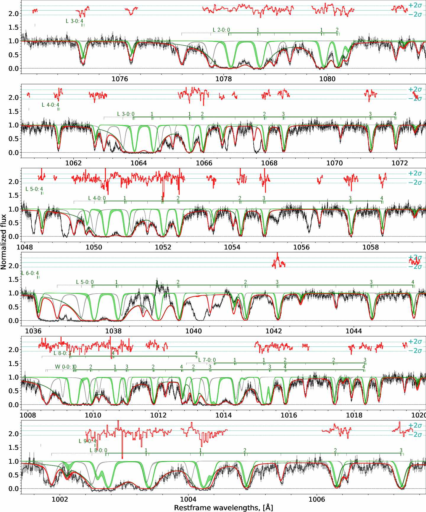
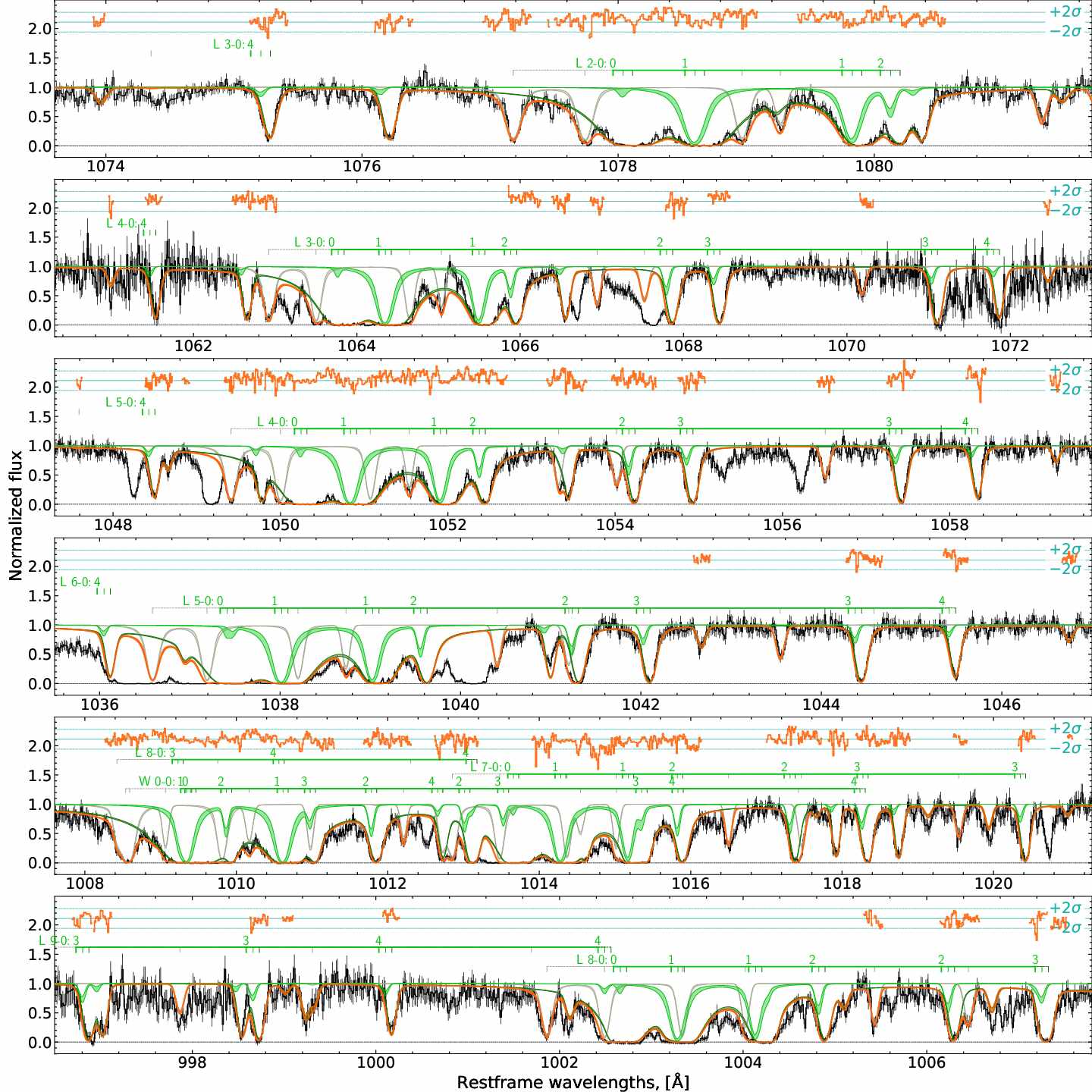
Firstly we refitted H₂ absorption lines, that typically corresponds to several lower rotational levels ($J\lesssim 5$) of the lowest vibrational state. In comparison with previous studies, where either only curve of growth analyses was used, or profiles were fitted only for the lower, $J=0,1$ levels, we performed the full joint profile fitting of all available levels. We used the same redshifts for all H₂ rotational levels, but allowed Doppler parameters to vary independently (except upper levels in several systems where the values were found to be unreasonably large). Additionally, we used the penalty functions (for details see, e.g. Noterdaeme et al., 2019; Kosenko et al., 2021) to favour a regular smooth shape of H₂ excitation diagram and an effect of increase of Doppler parameters with an increase of J, as was noticed before Balashev et al. 2009, e.g.; Noterdaeme et al. 2007, e.g..

The nominal resolution of spectra, obtained by FUSE is $R=\lambda/\Delta\lambda=20000$, but we noticed that it can be reduced by a procedure of exposure coadding, calibration and other systematic effects of observations. So we made $R$ to be an additional independent parameter during the fitting procedure. In the most cases, we found $R$ below 20000, in the range $\sim 11000-18000$.

Using obtained velocity decomposition from H₂ profiles, we constrained the column density of HD molecules at the position of H₂ components. To fit HD column density we used priors on Doppler parameters from H₂ $\rm J=0$ (except systems where we detected HD) and fixed redshifts. One should note that many HD lines are blended, mostly by H₂, but also by metals; moreover some blends are attributed to the stellar absorptions.

4 Results

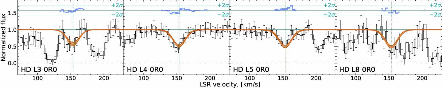
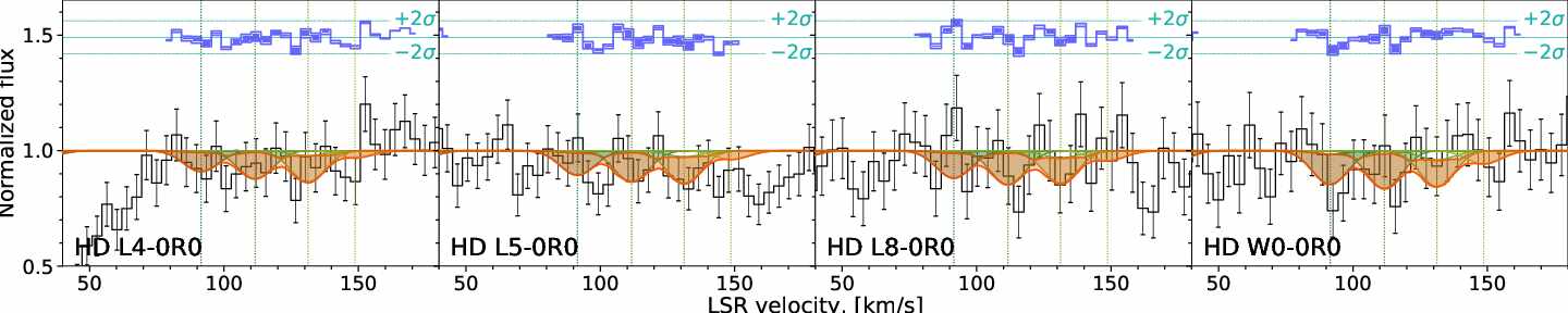
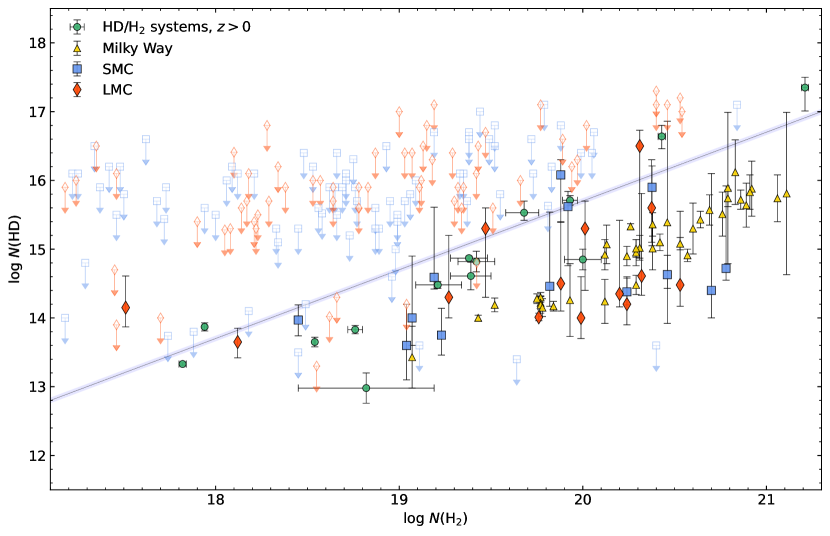
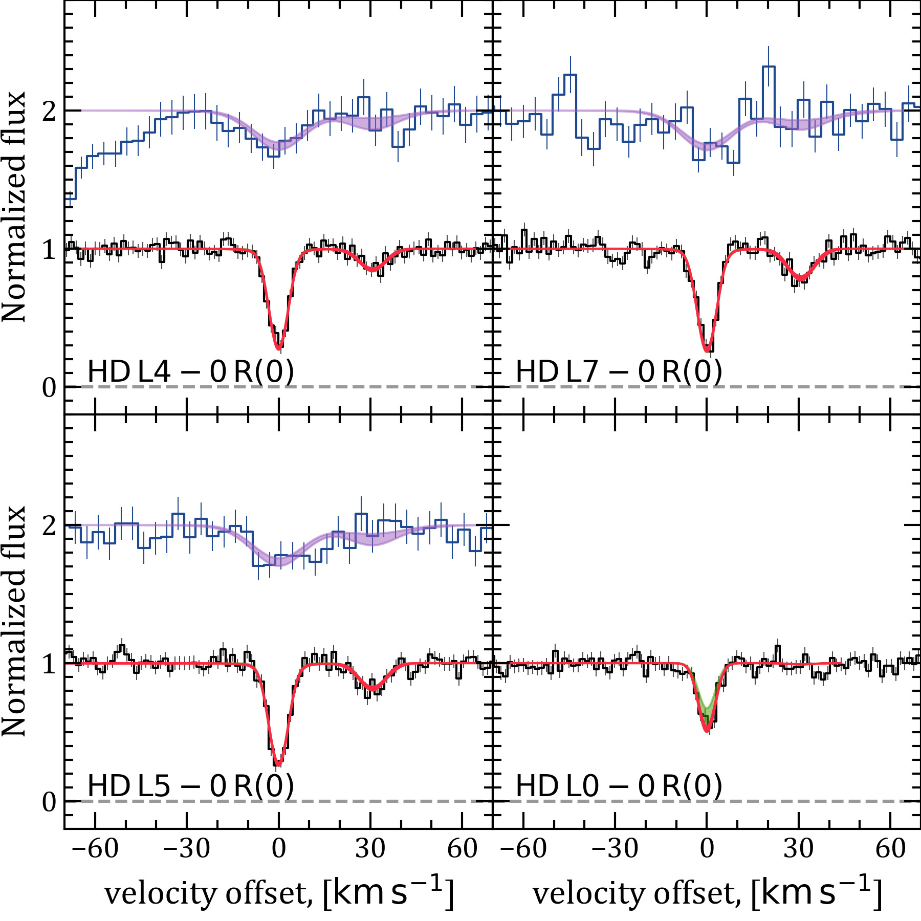
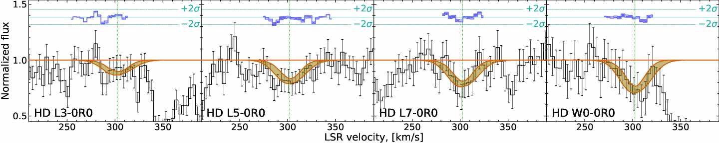
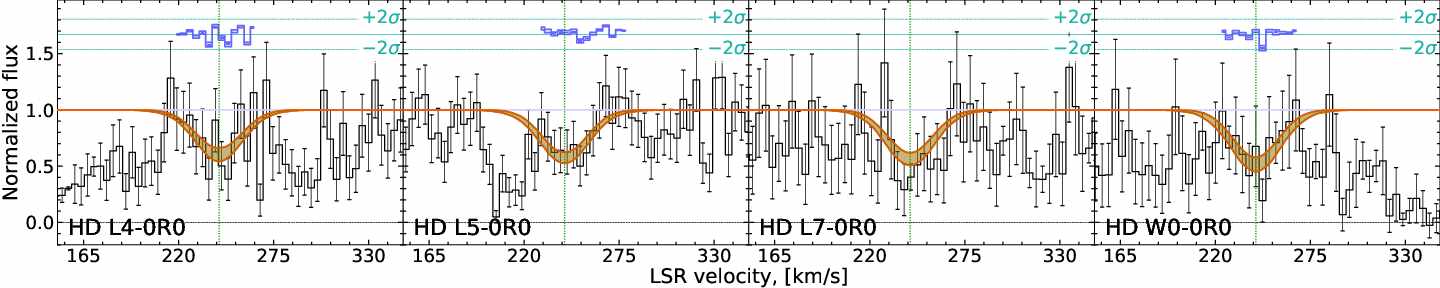
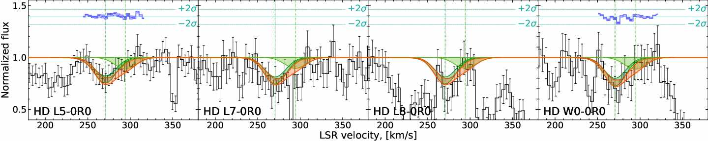
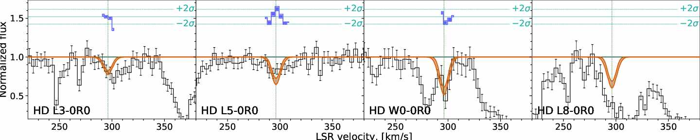
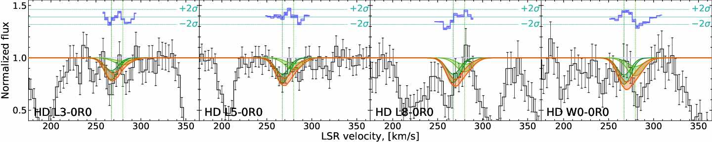
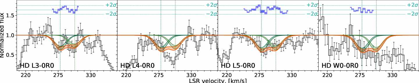
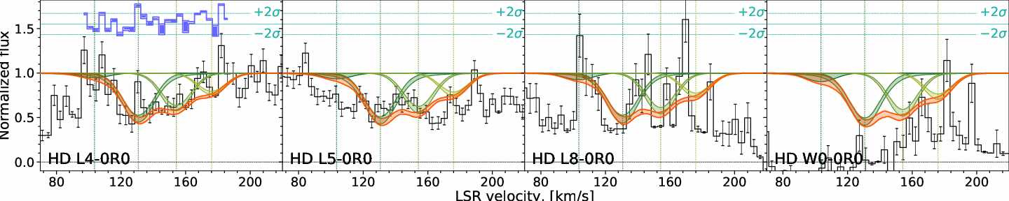
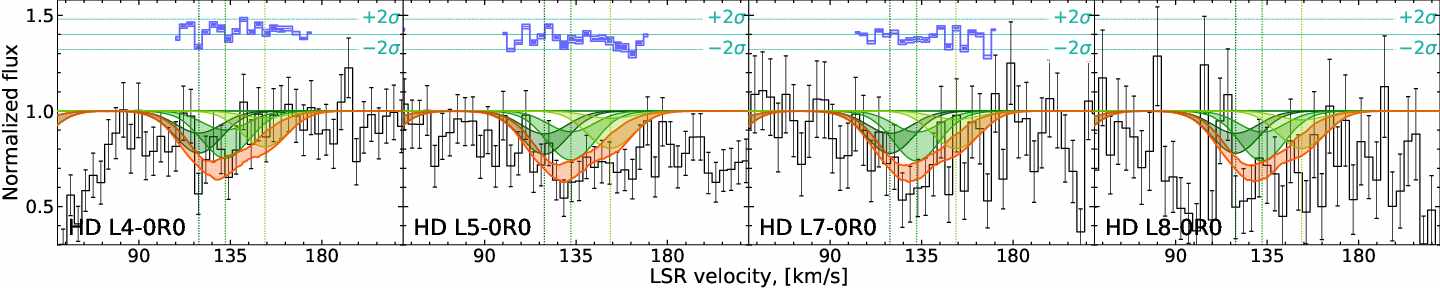
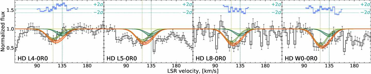
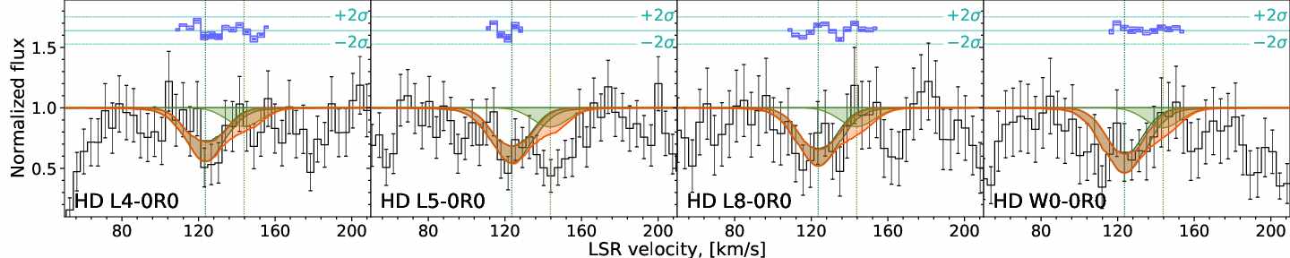
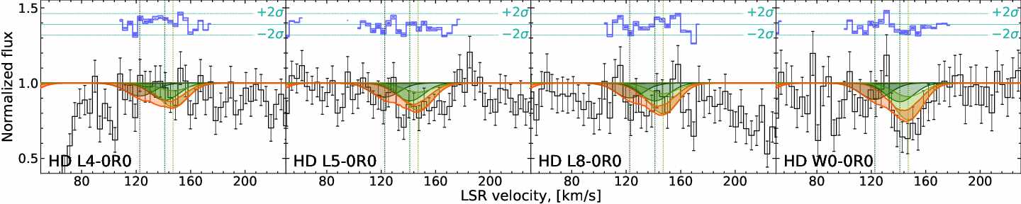
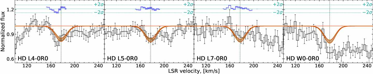
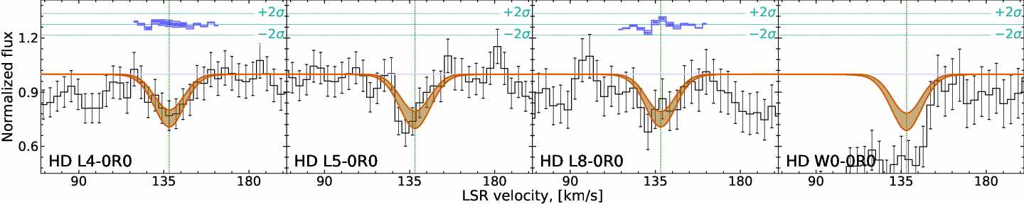
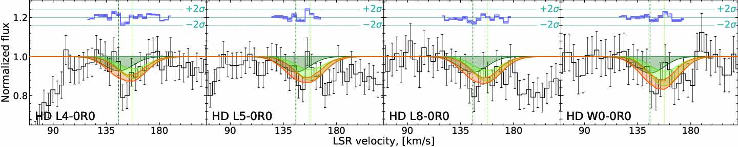
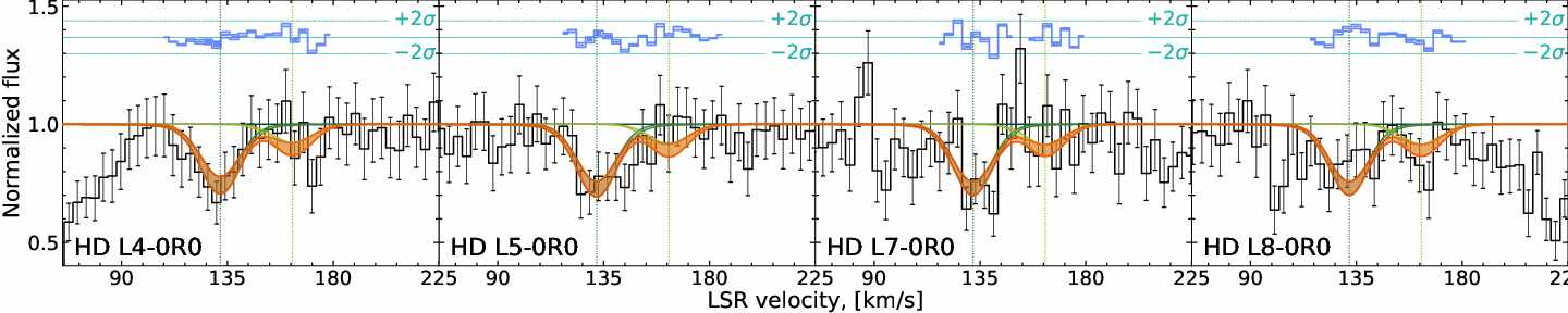
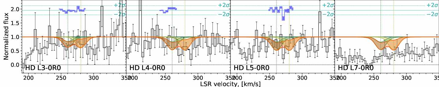
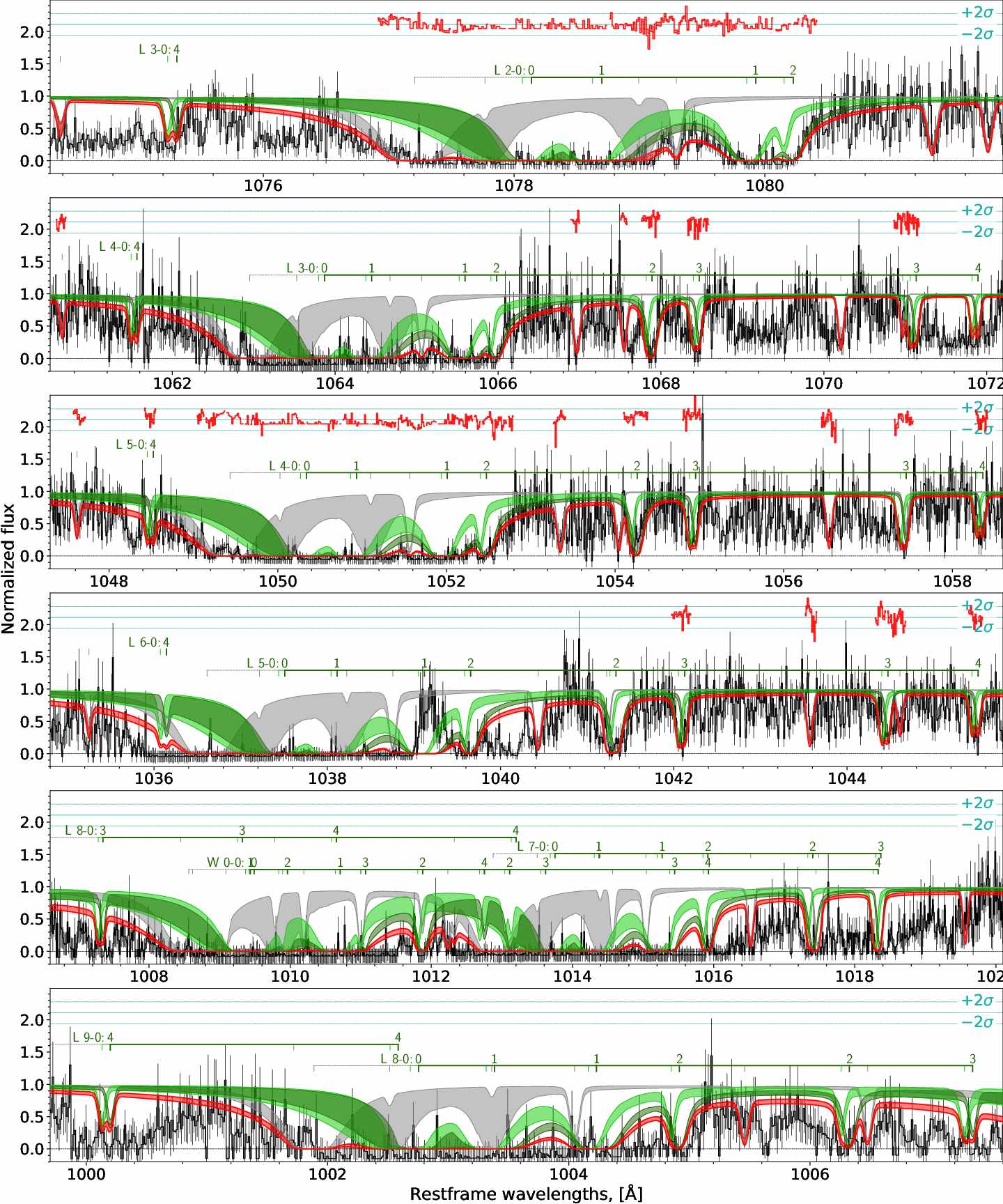
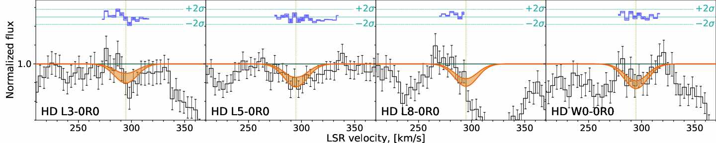
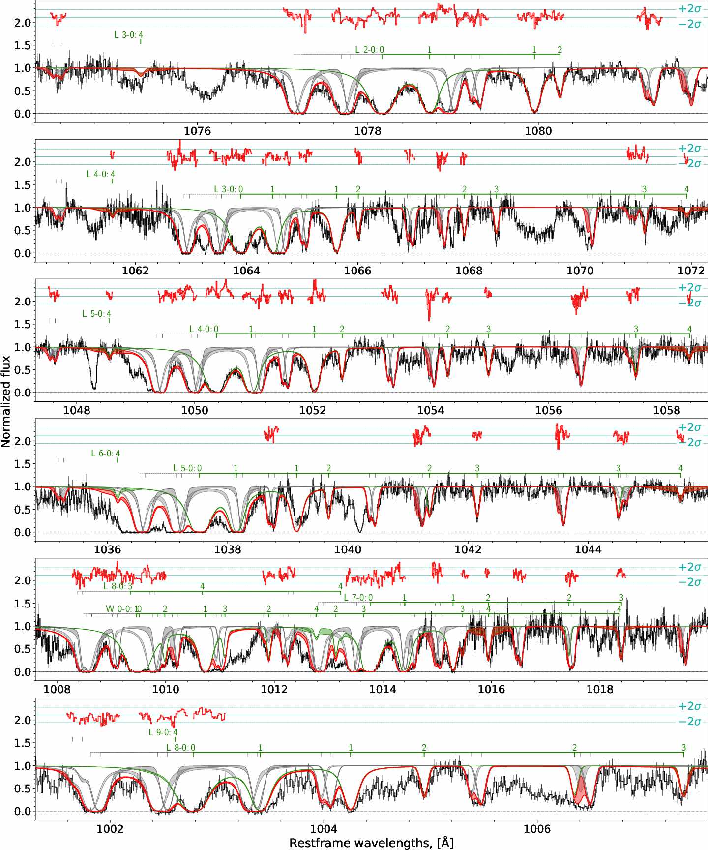
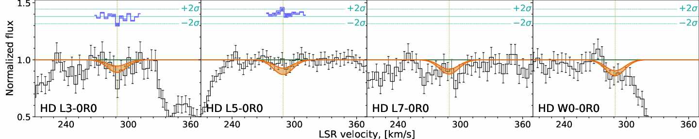
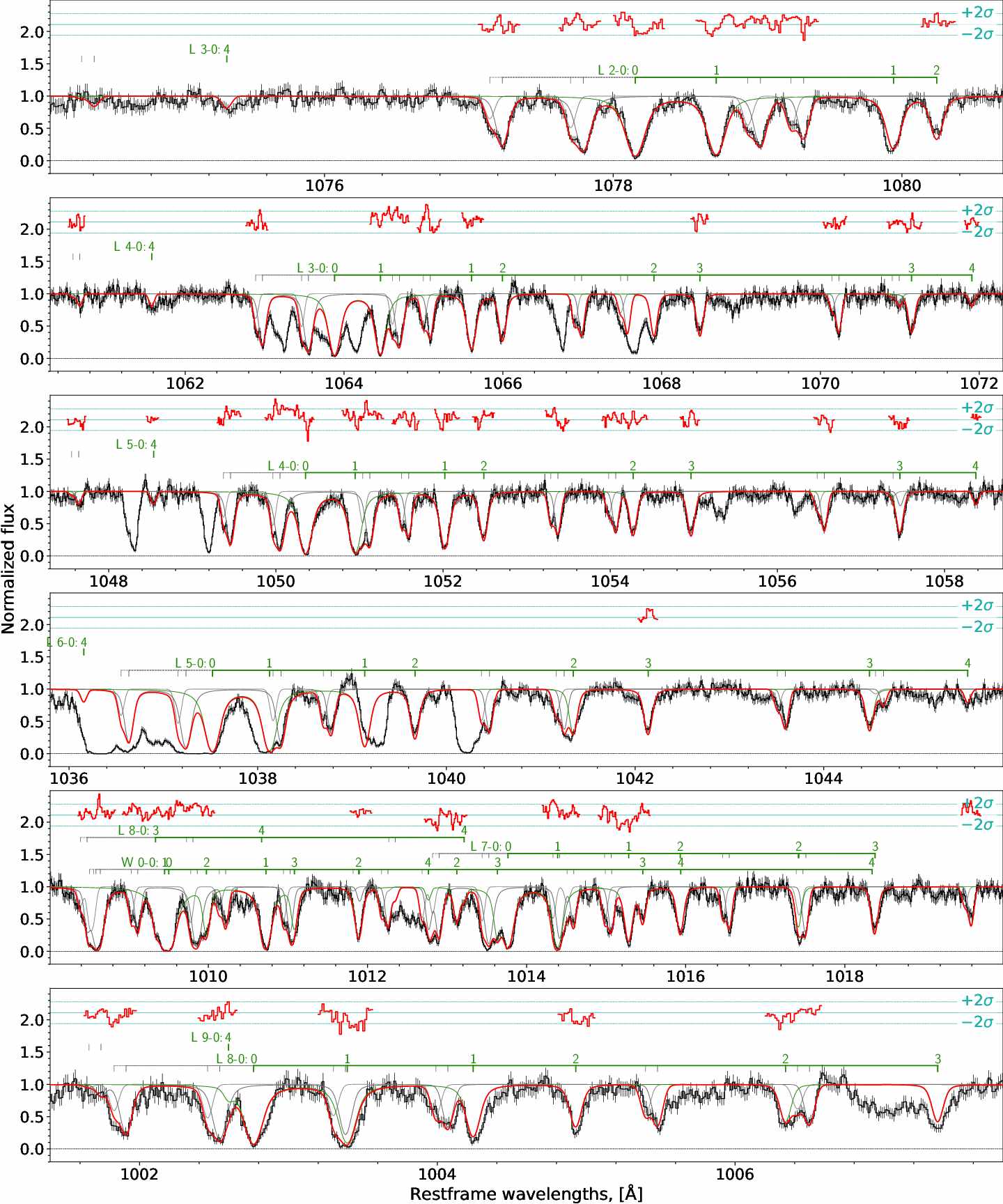
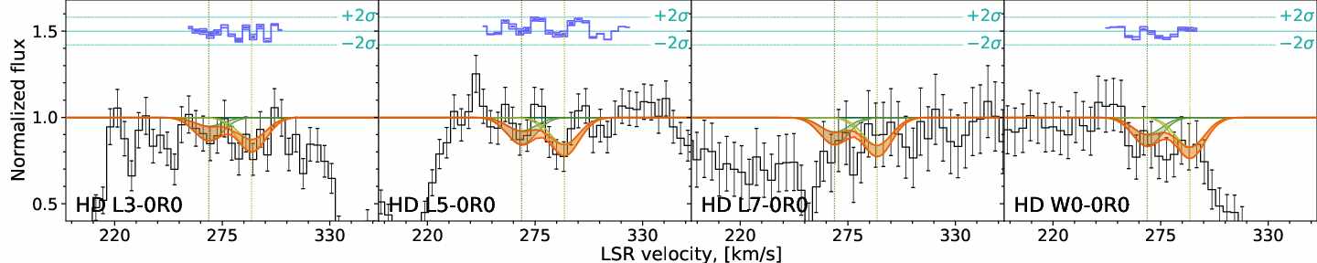
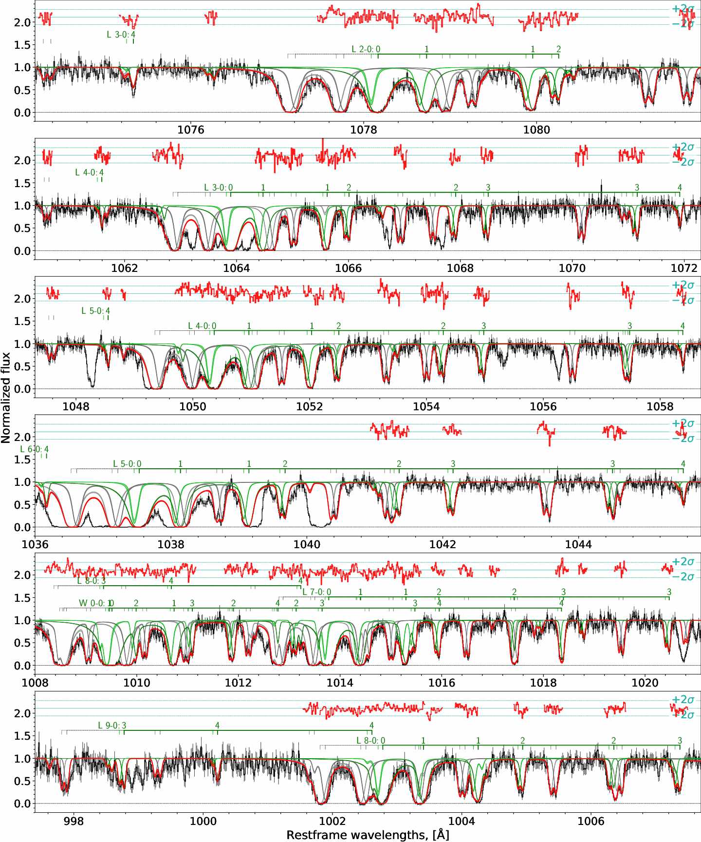
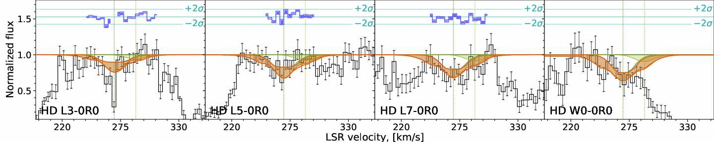
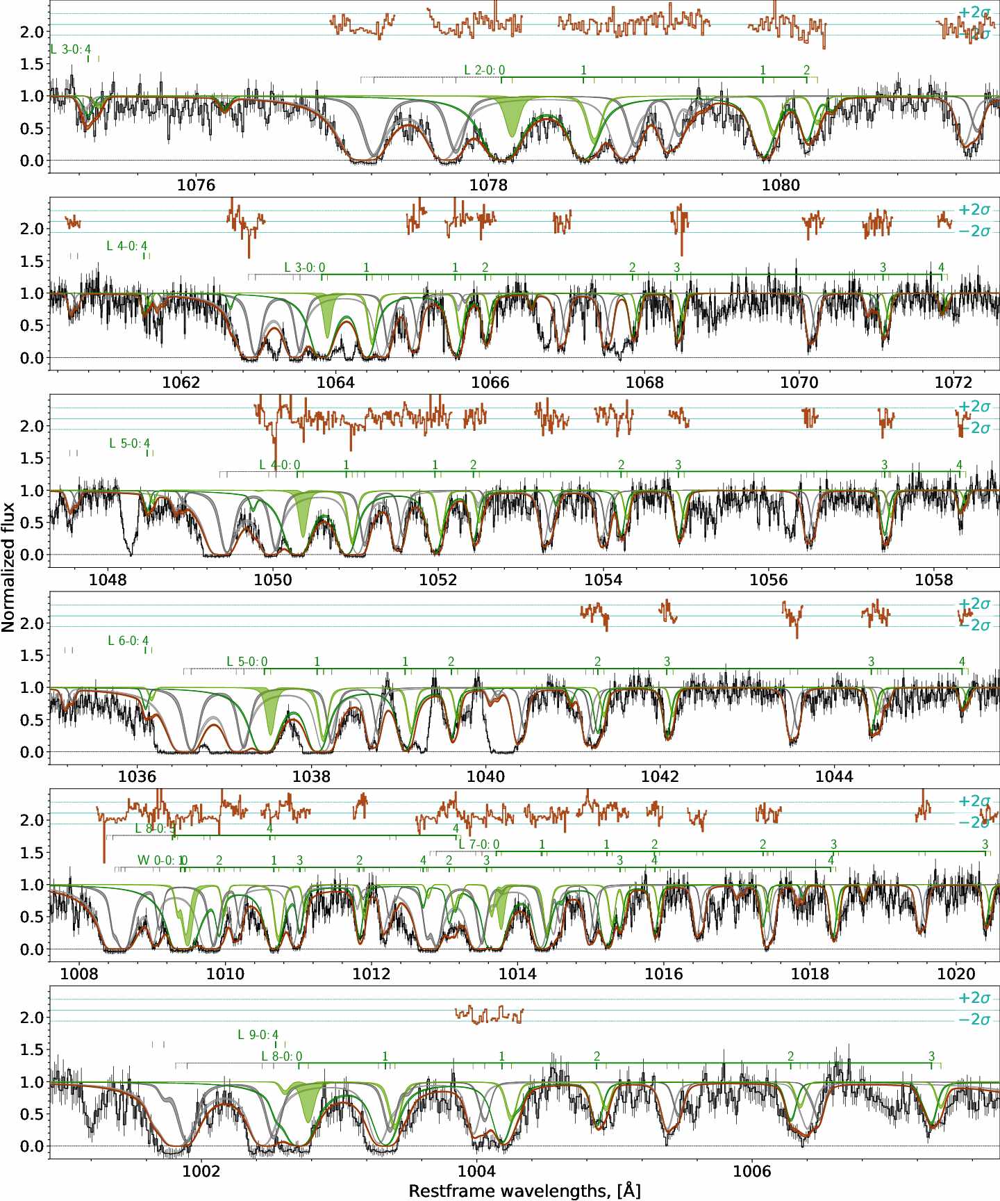
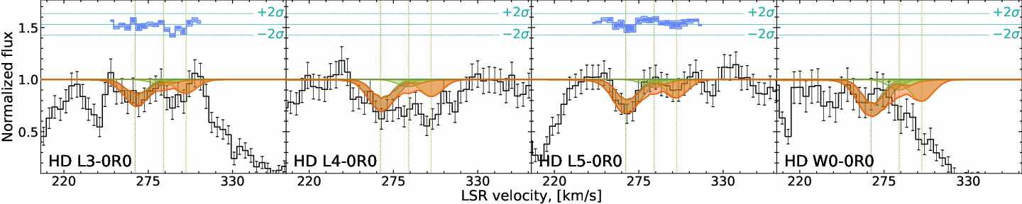
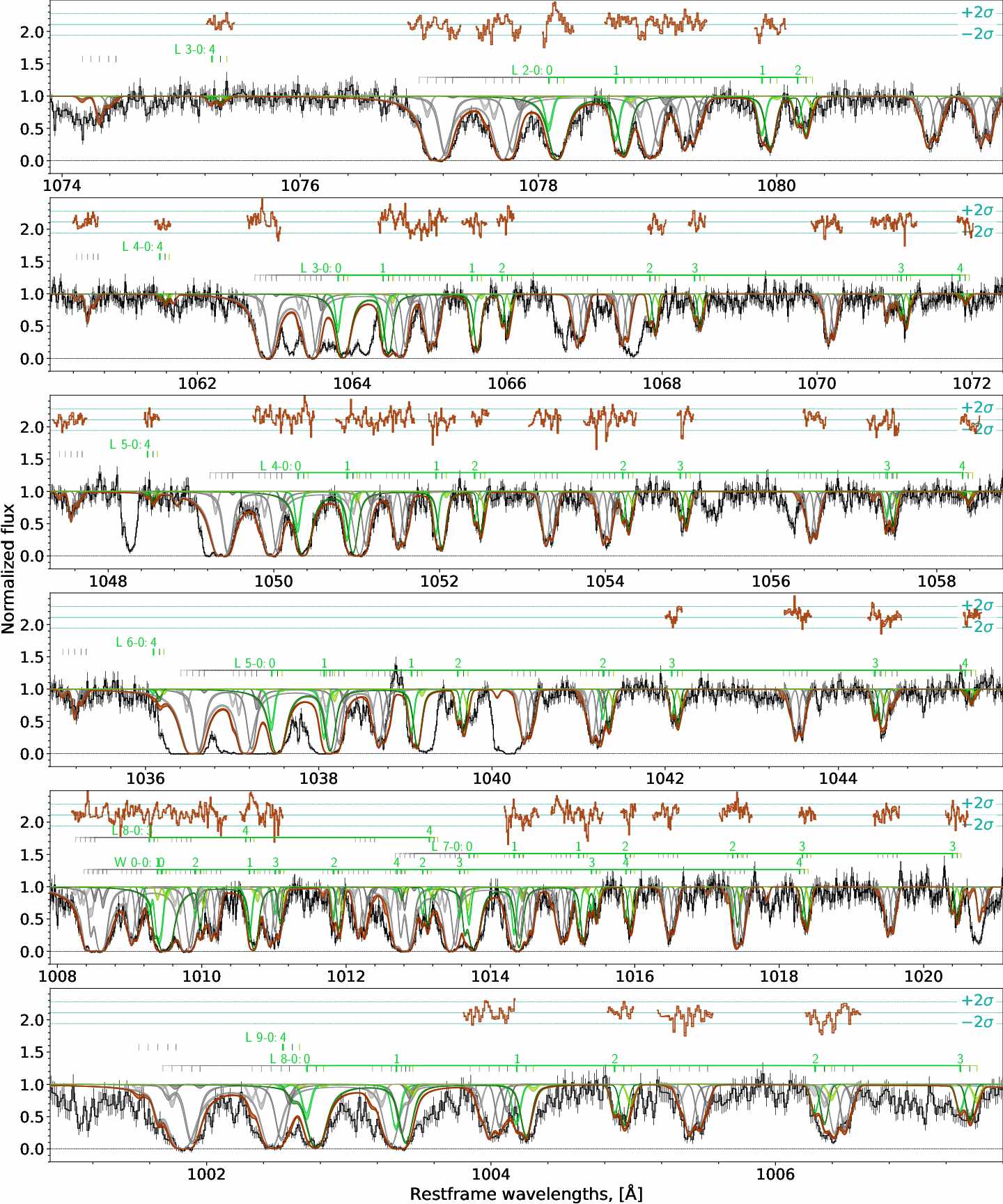
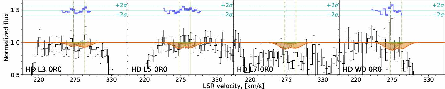
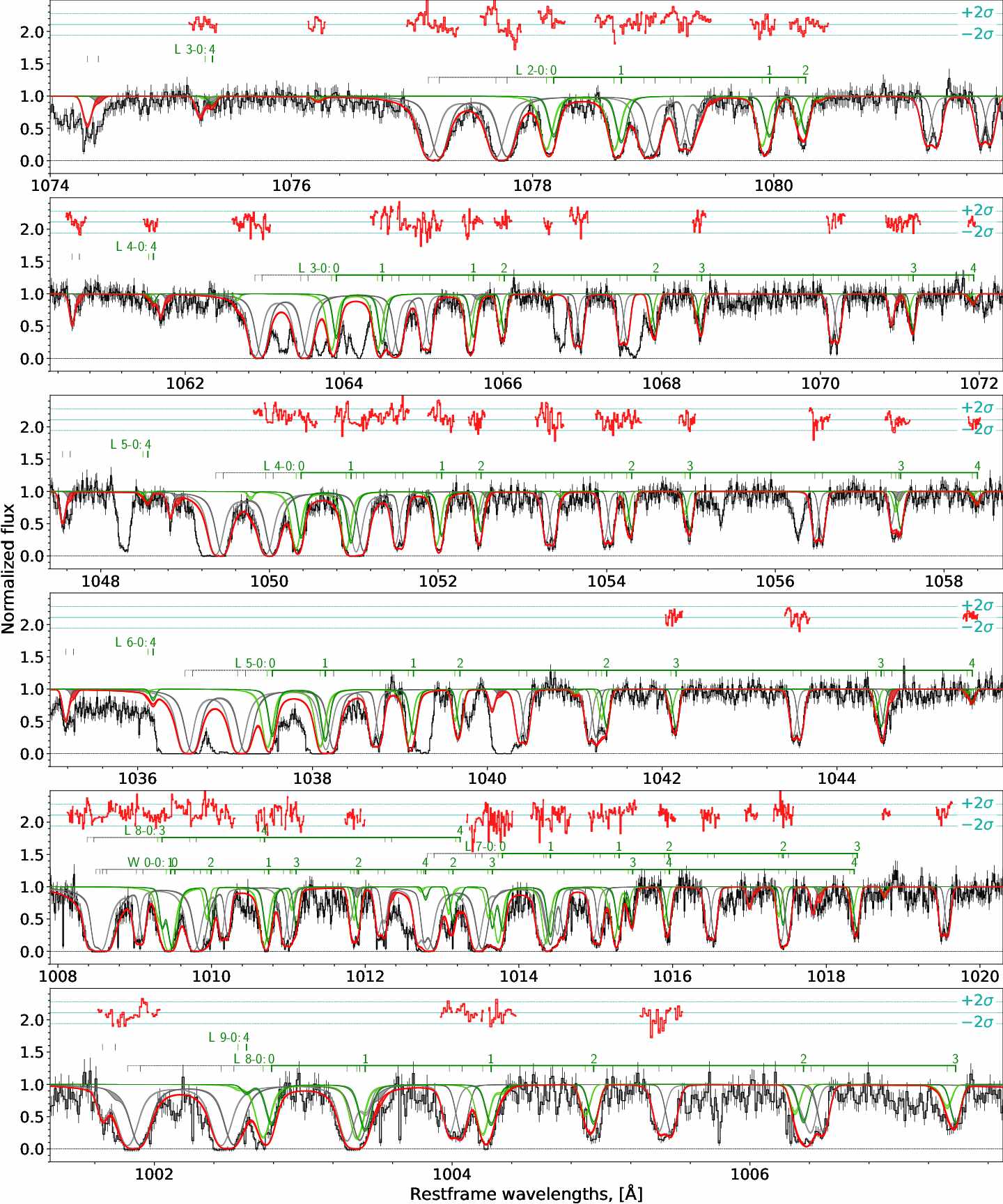
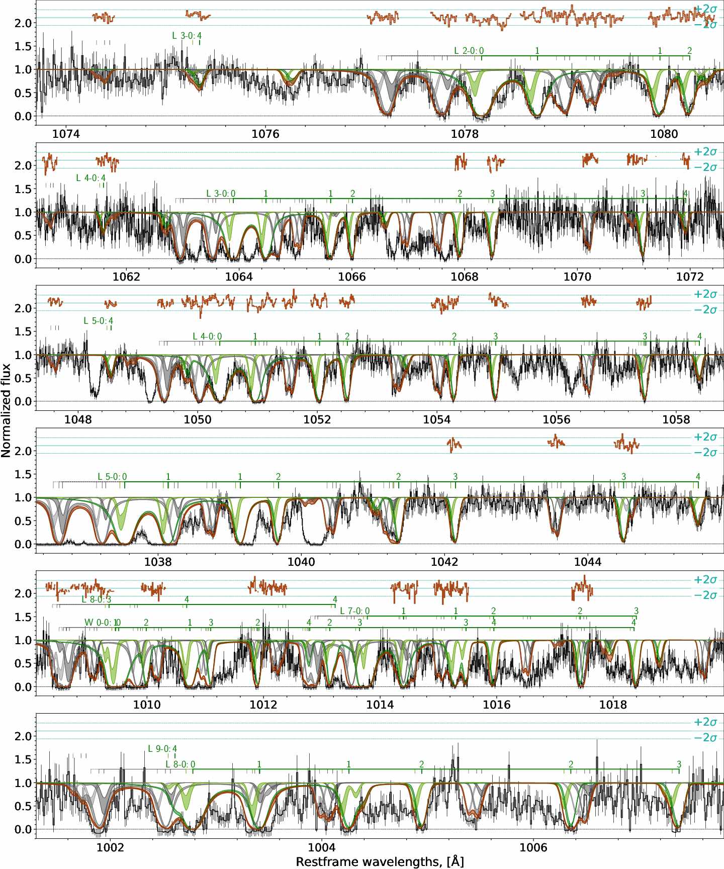
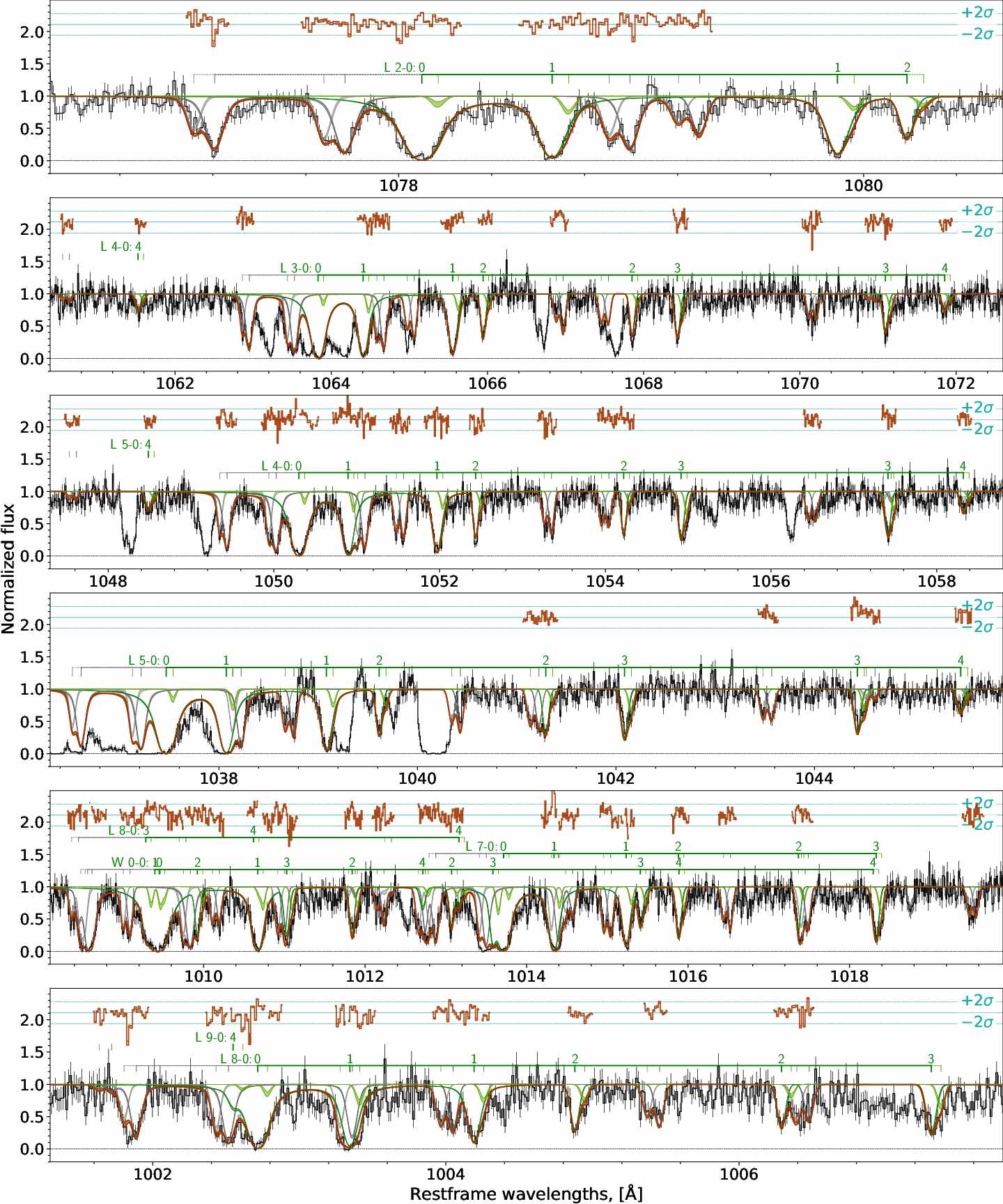
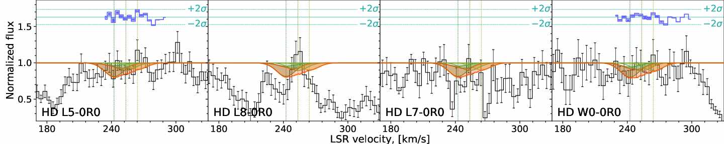
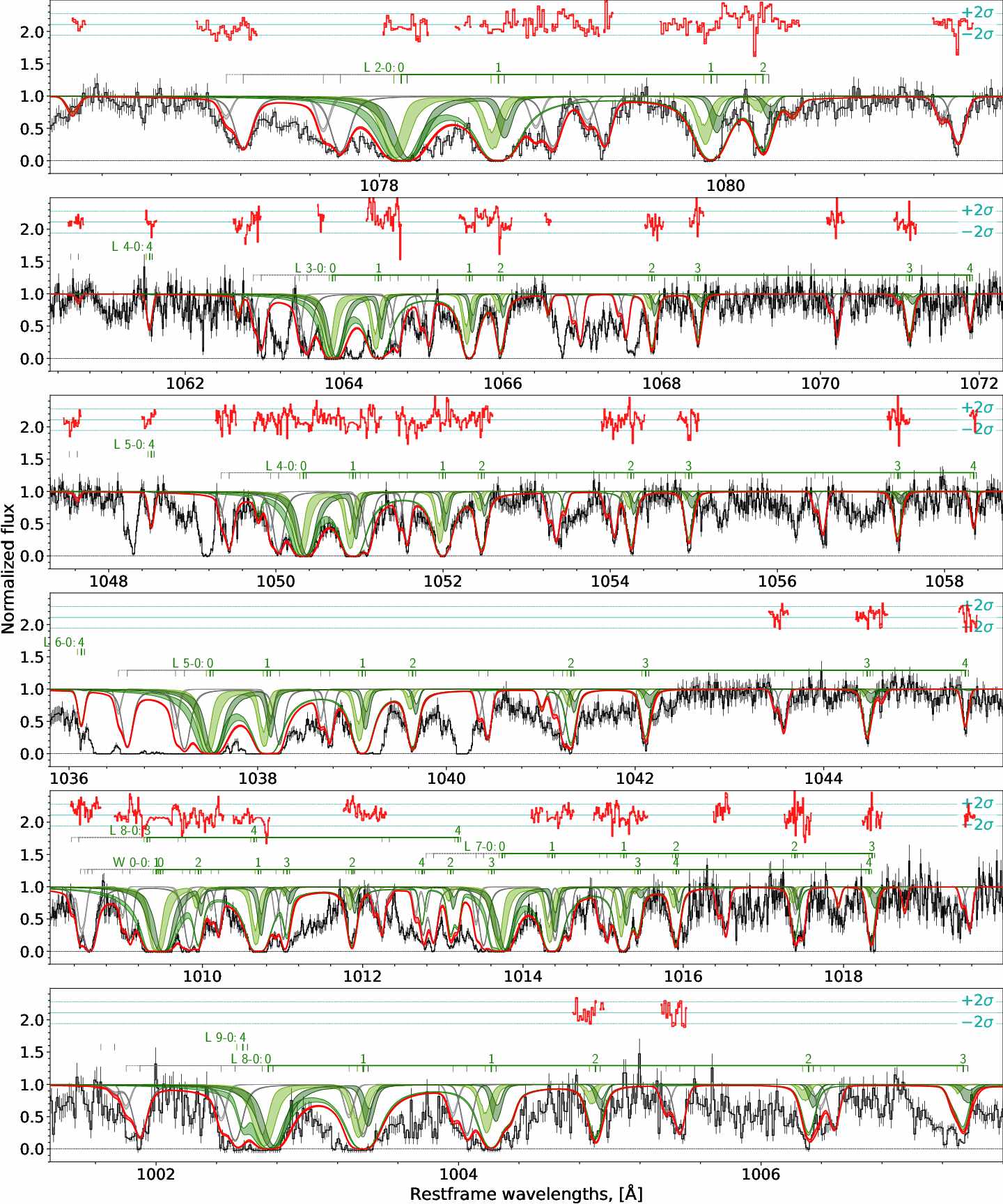
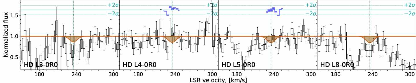
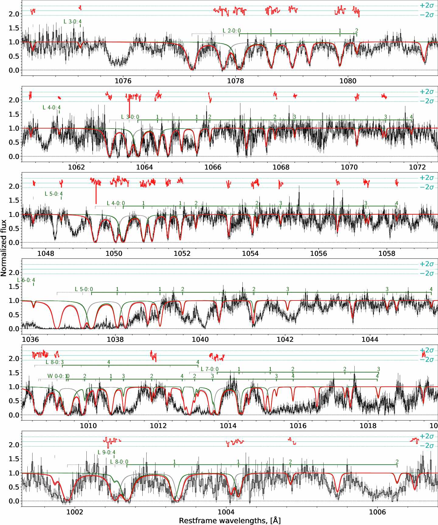
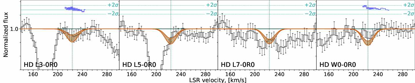
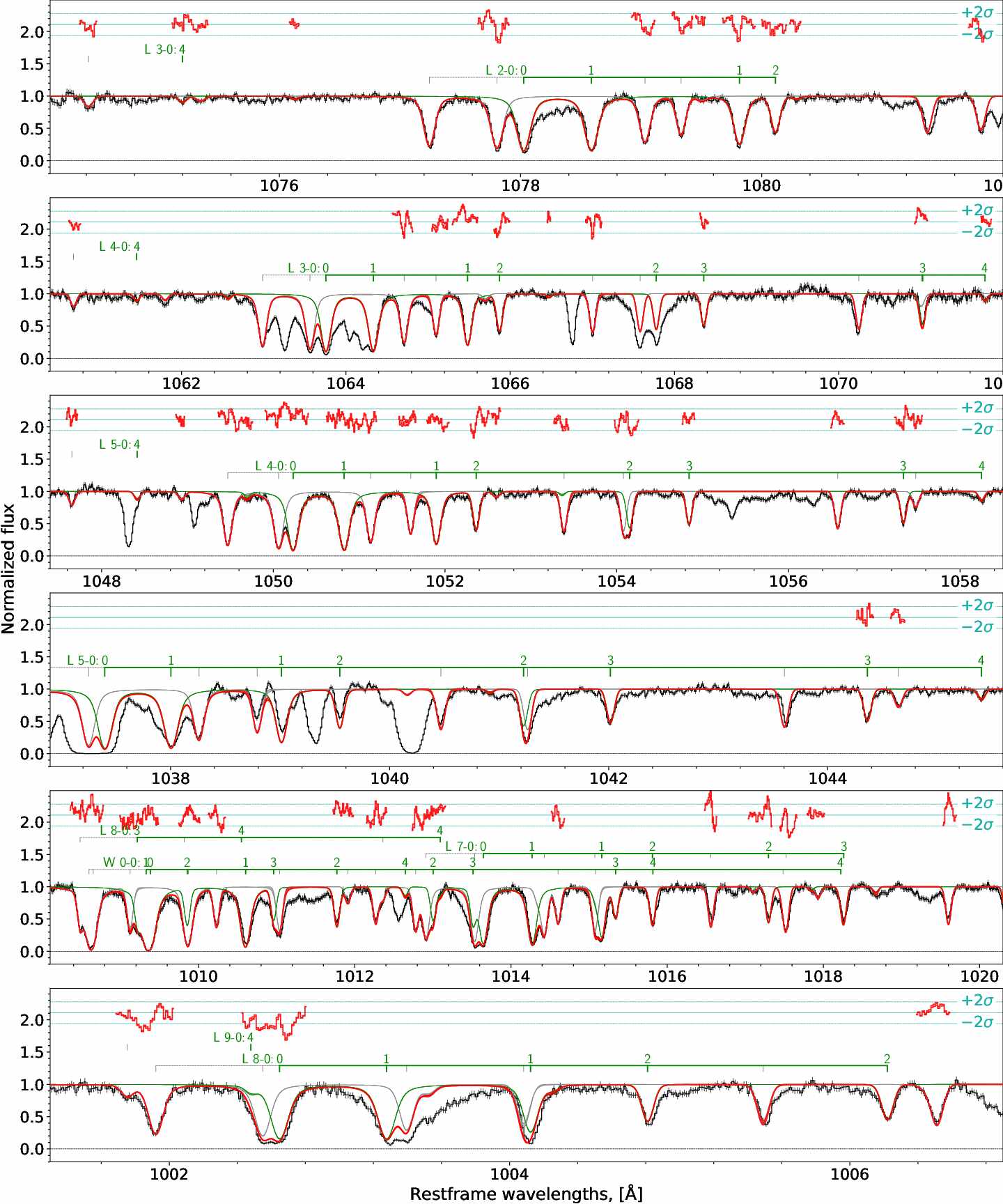
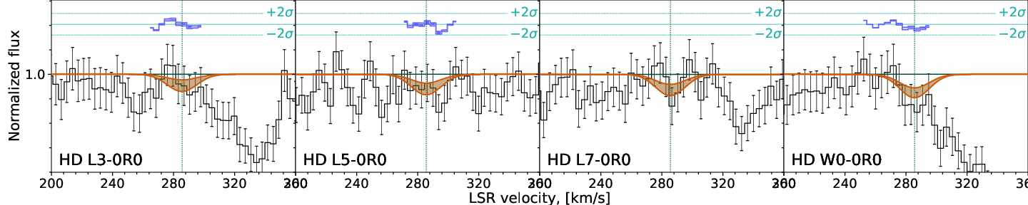
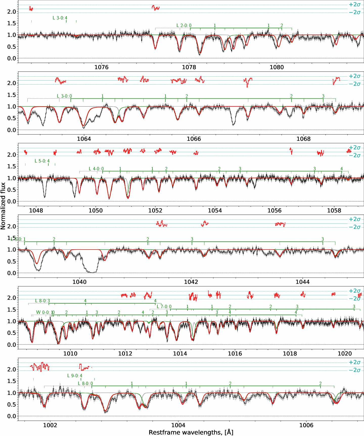
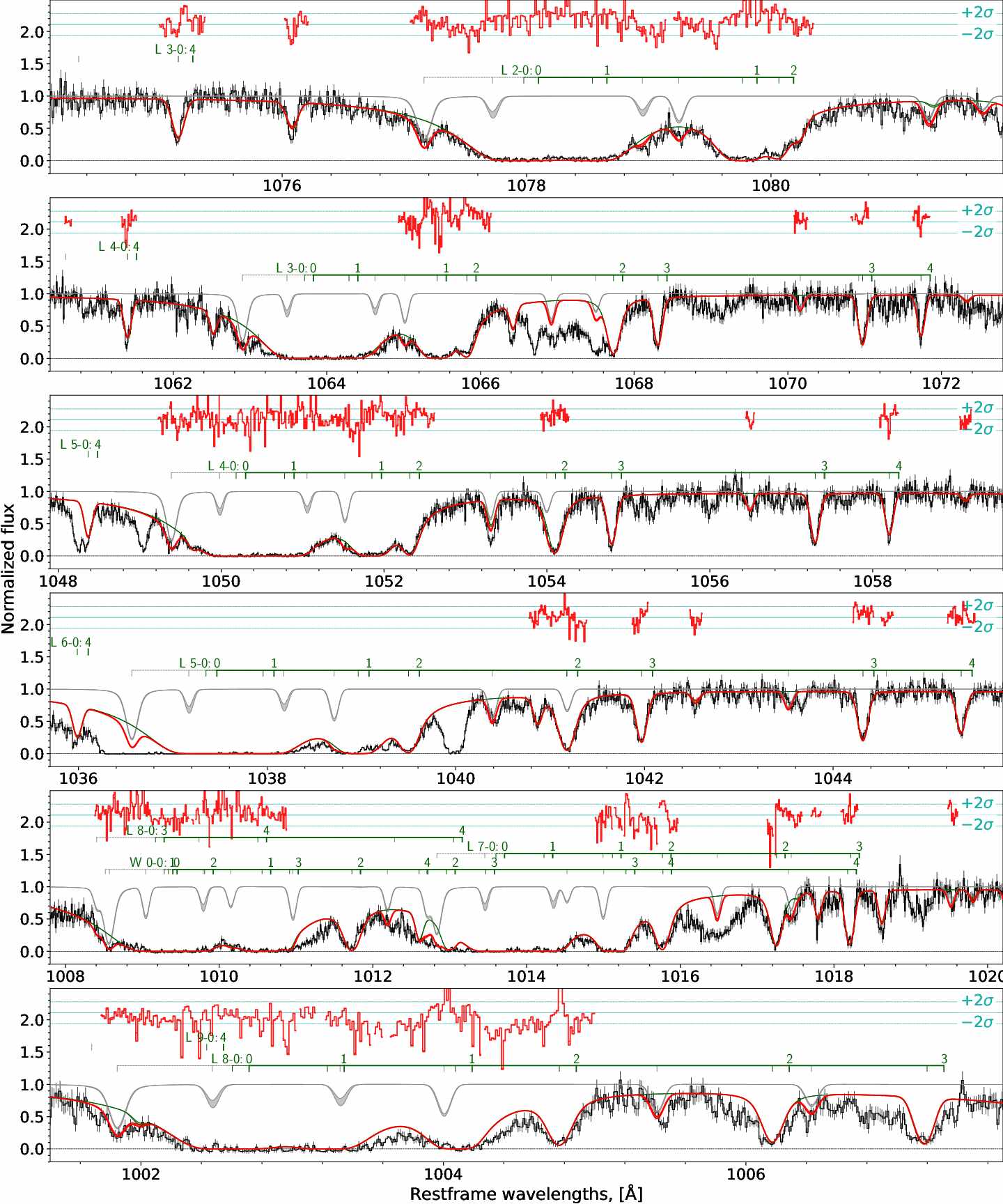
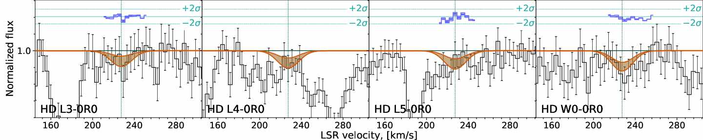
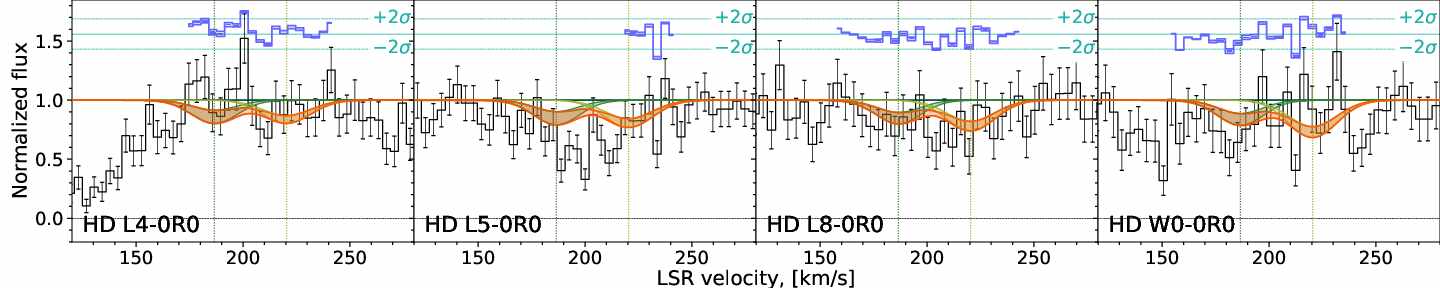
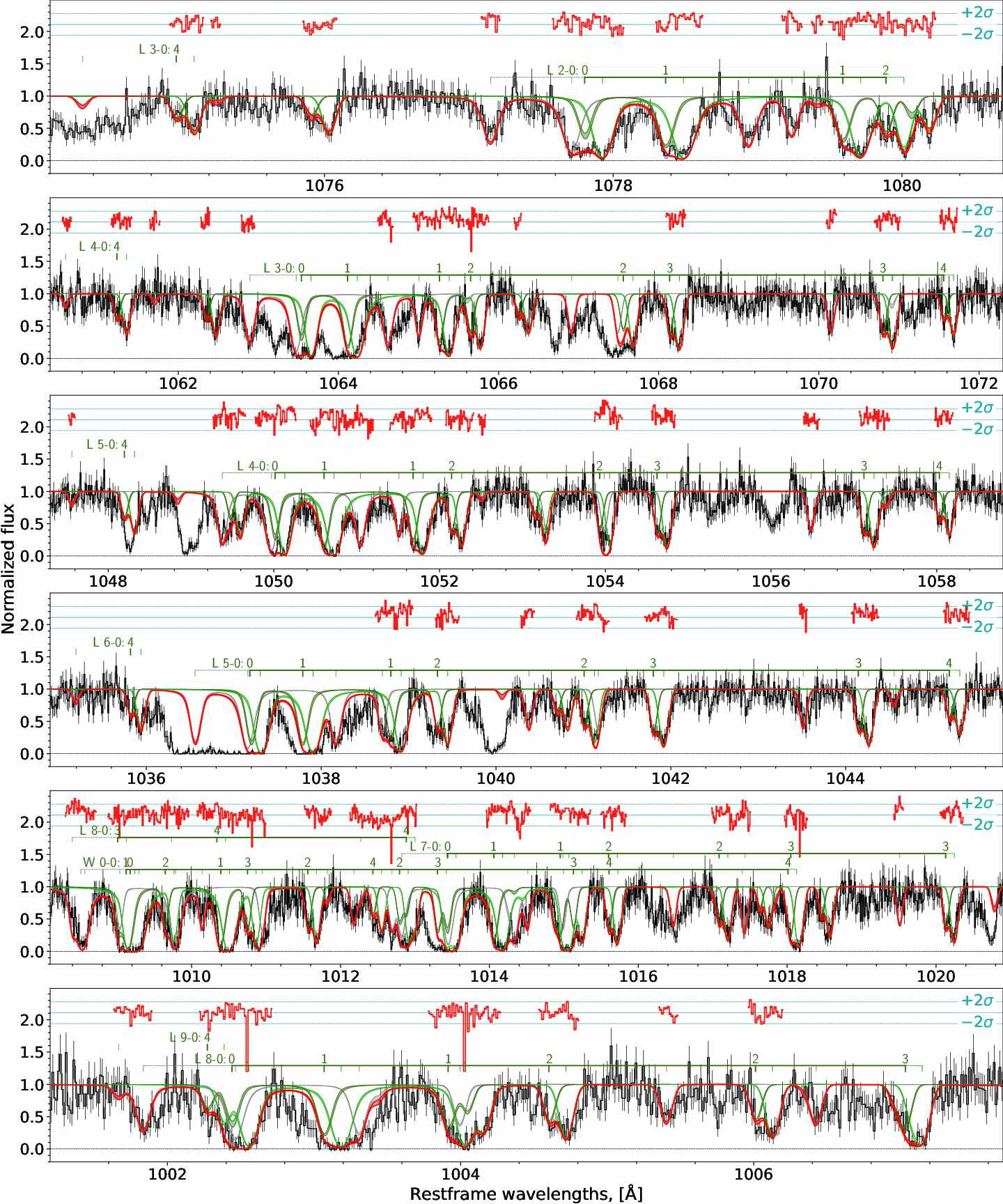
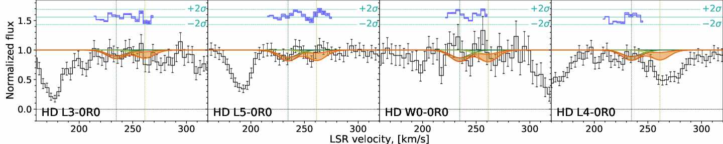
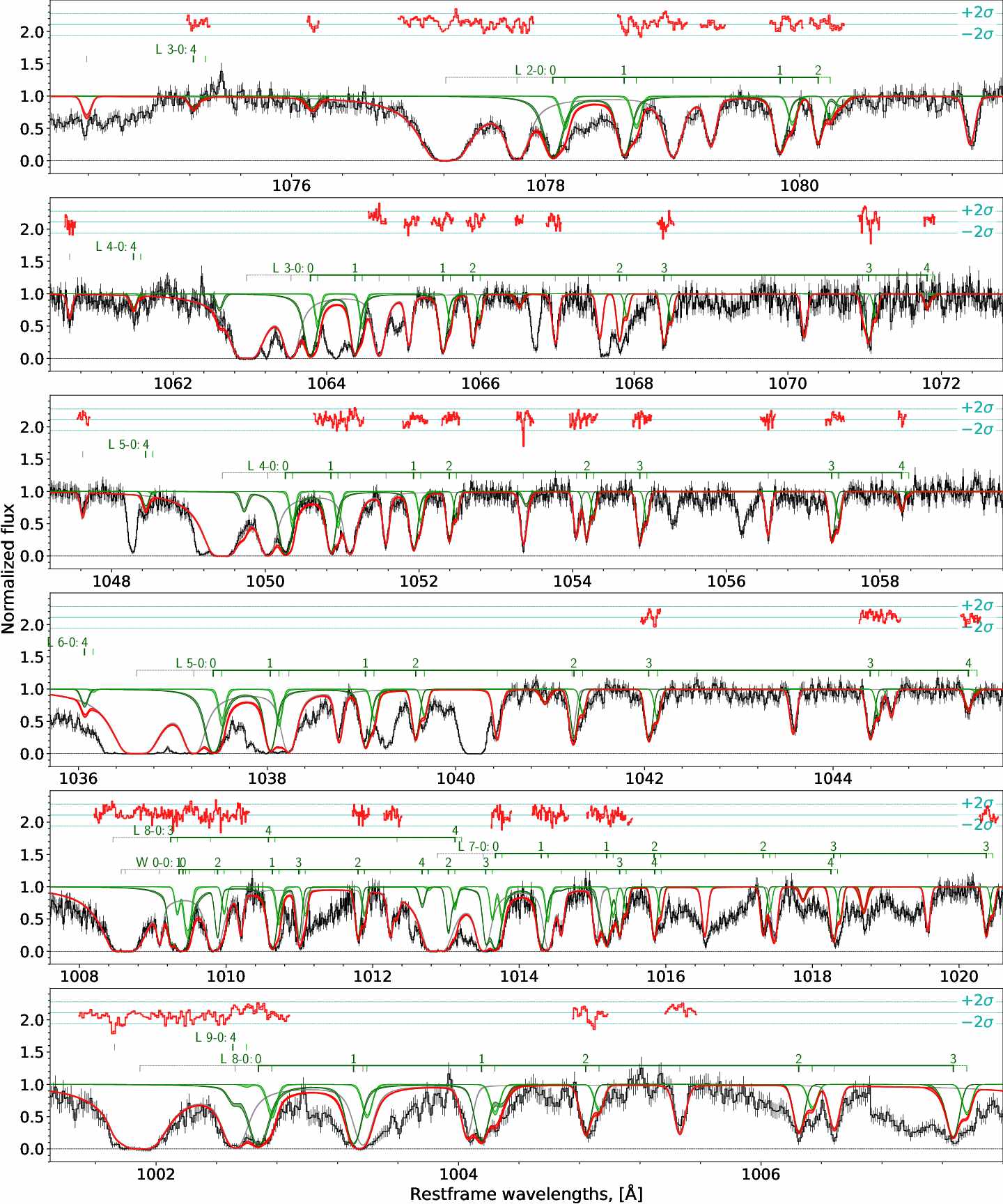
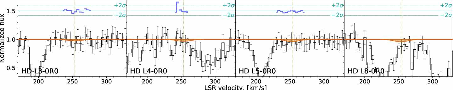
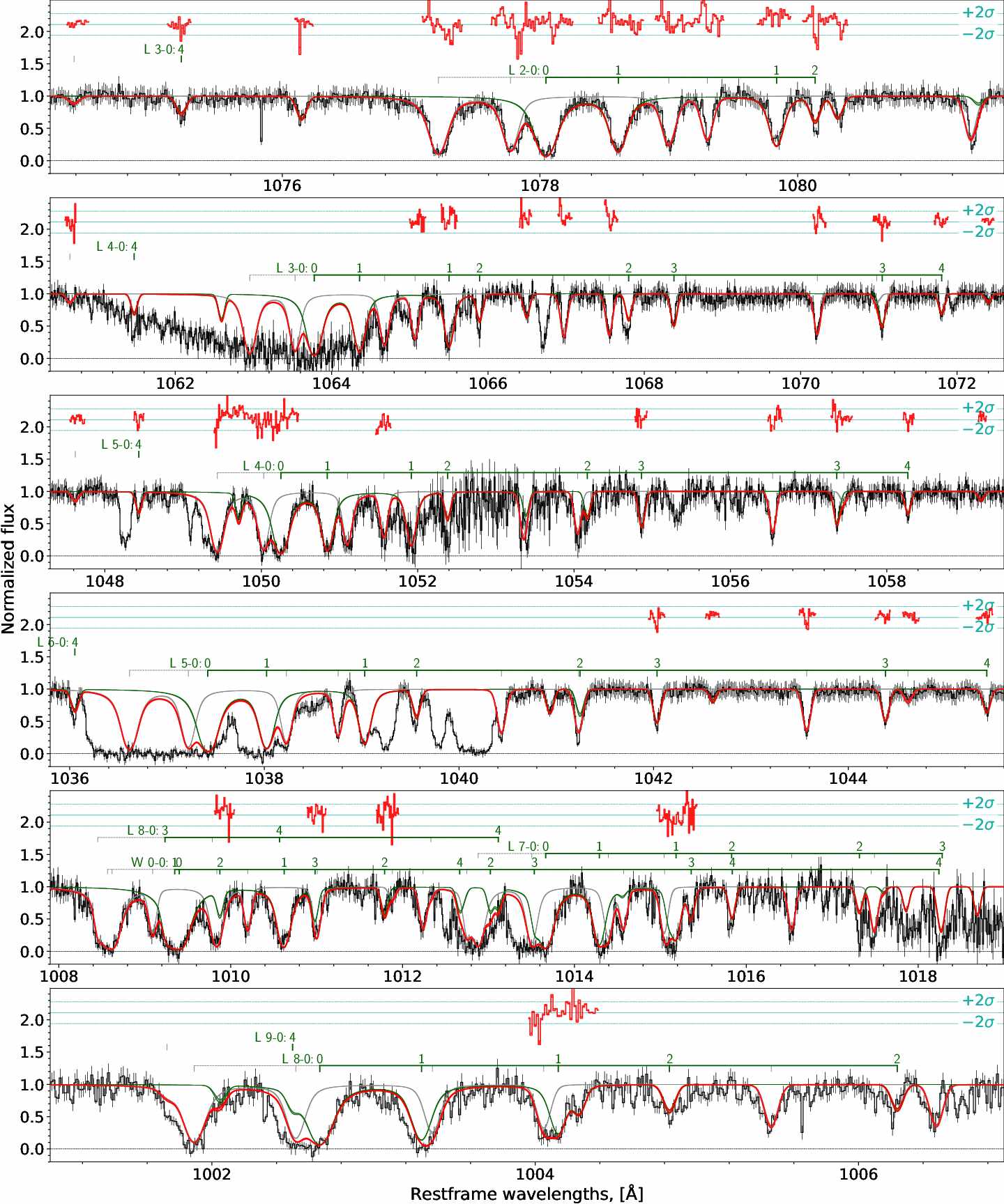
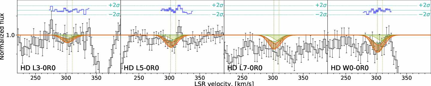
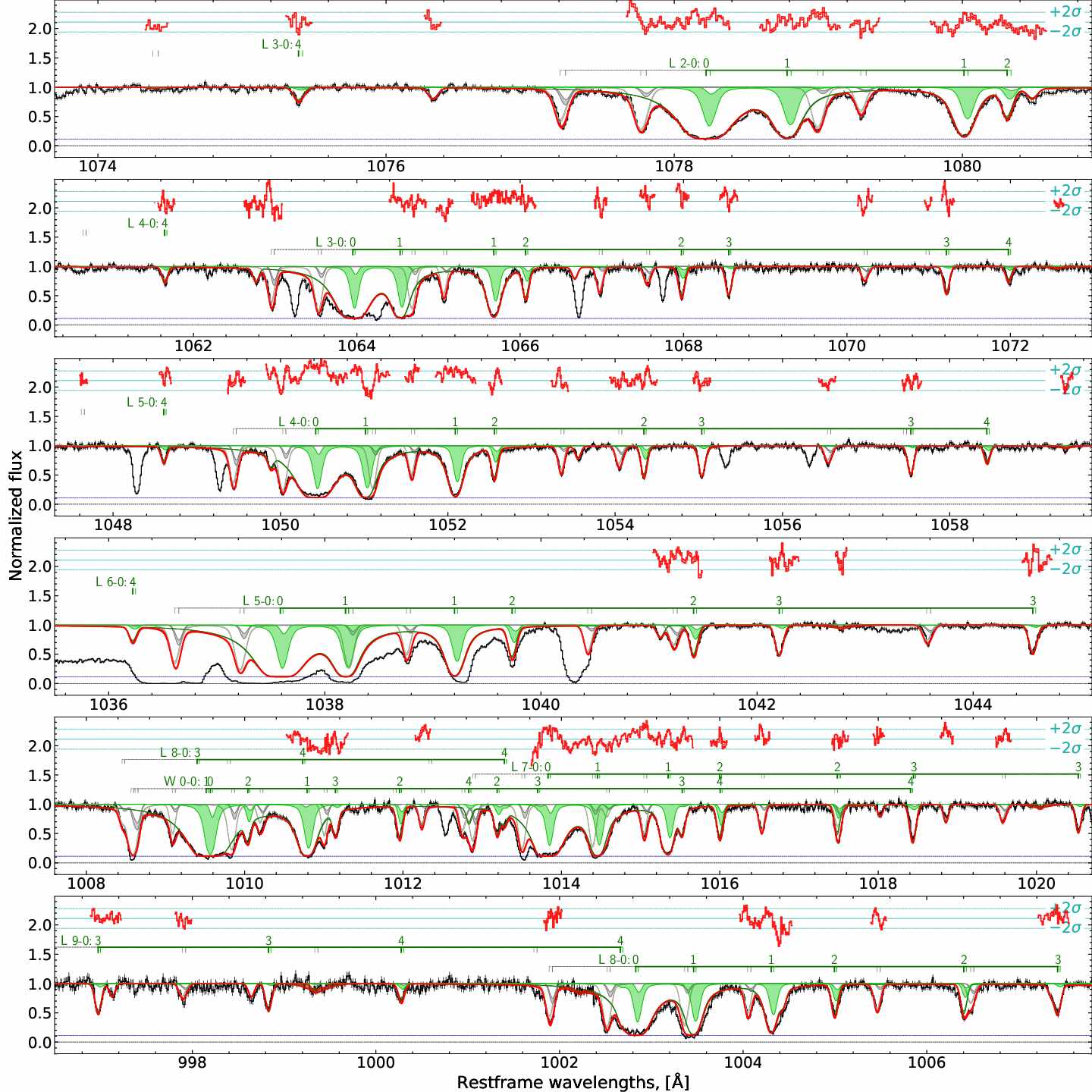
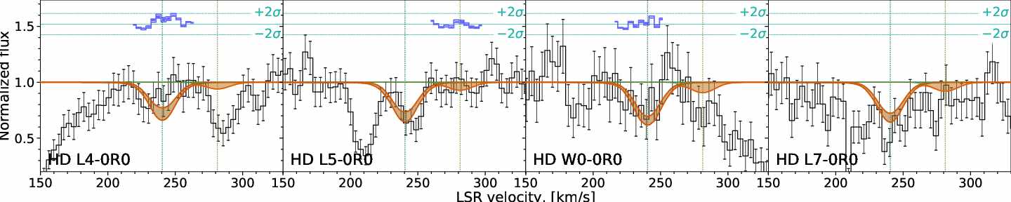
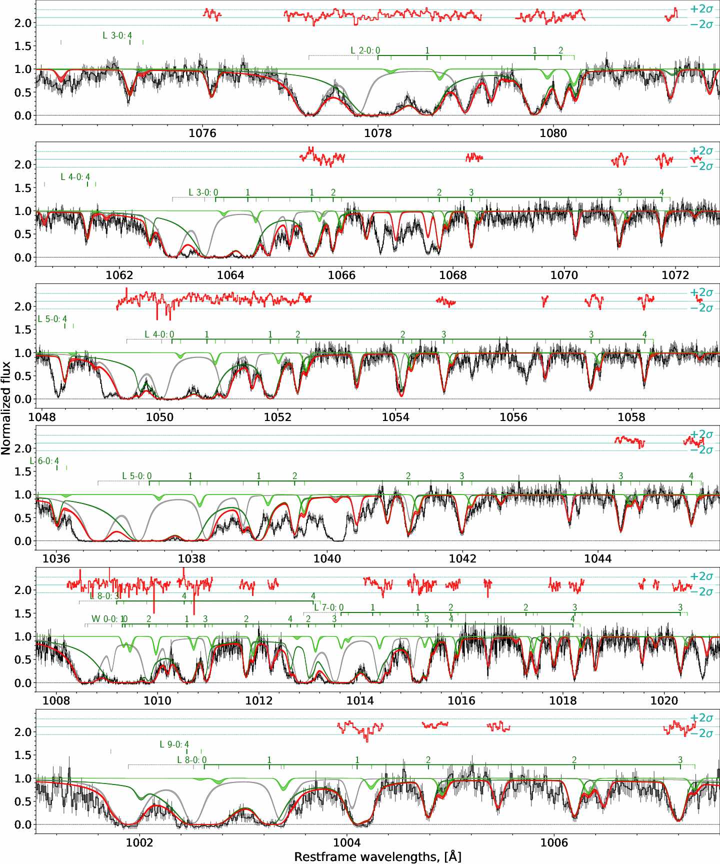
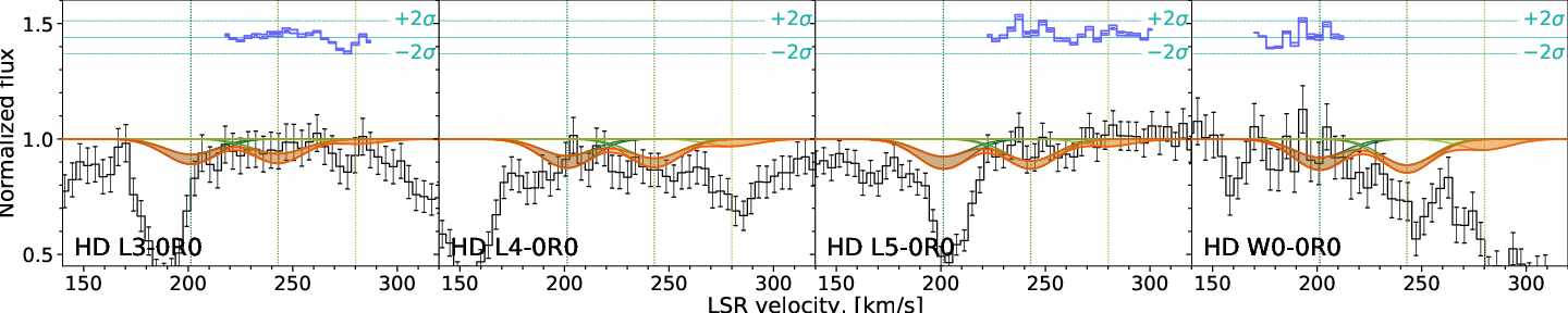
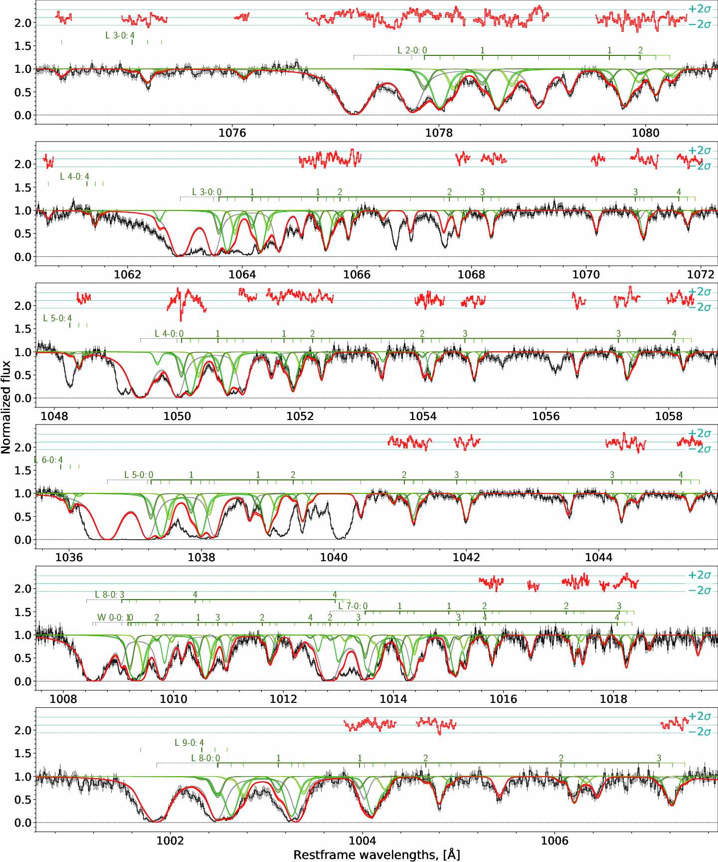
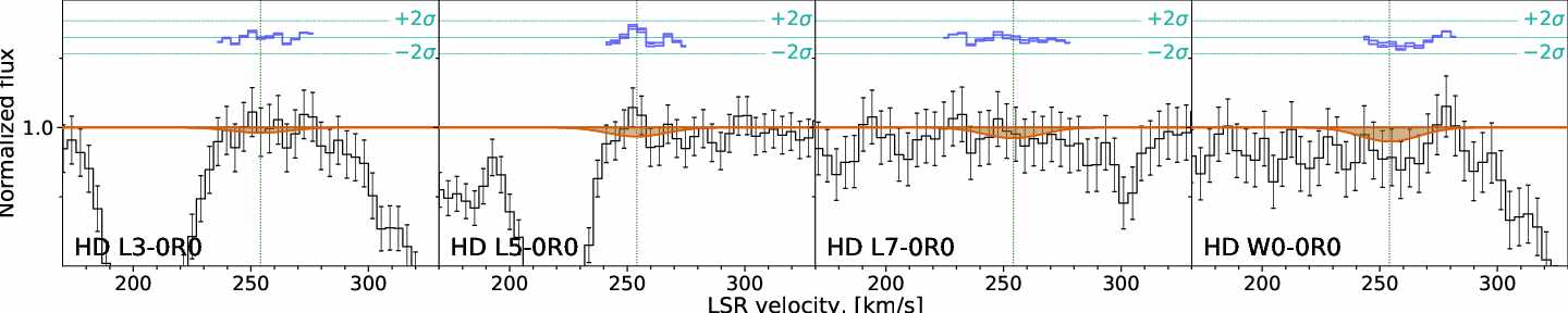
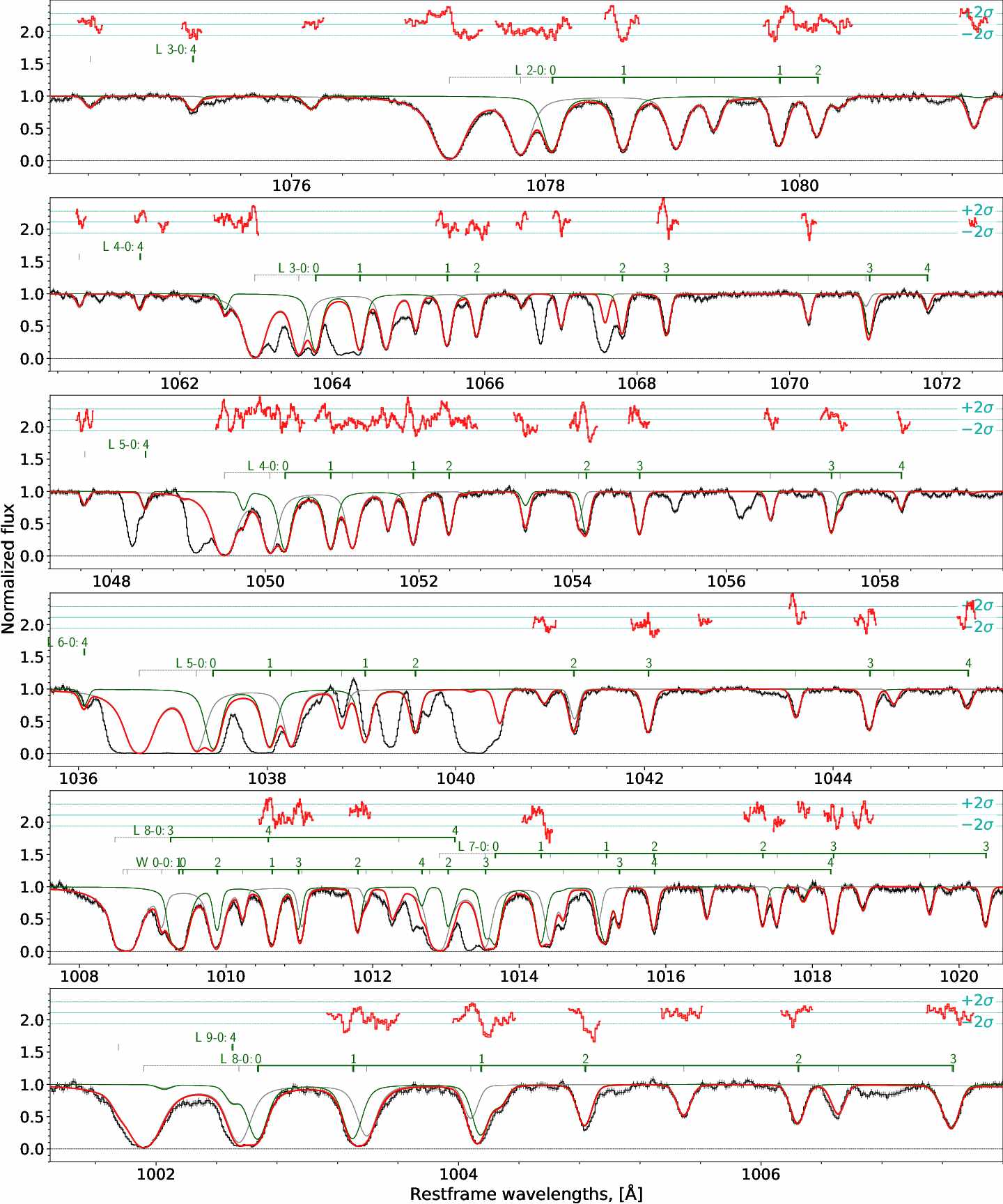
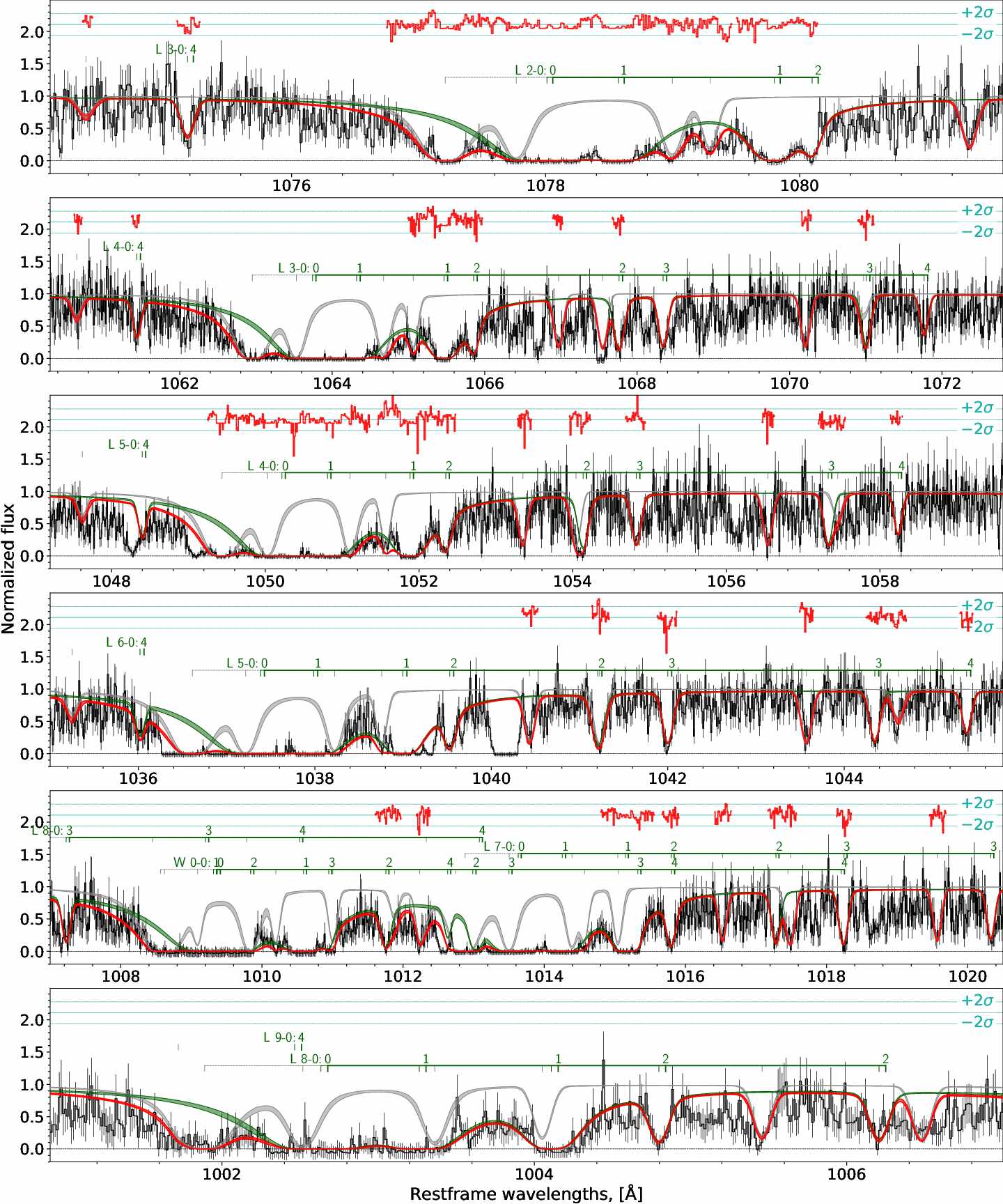
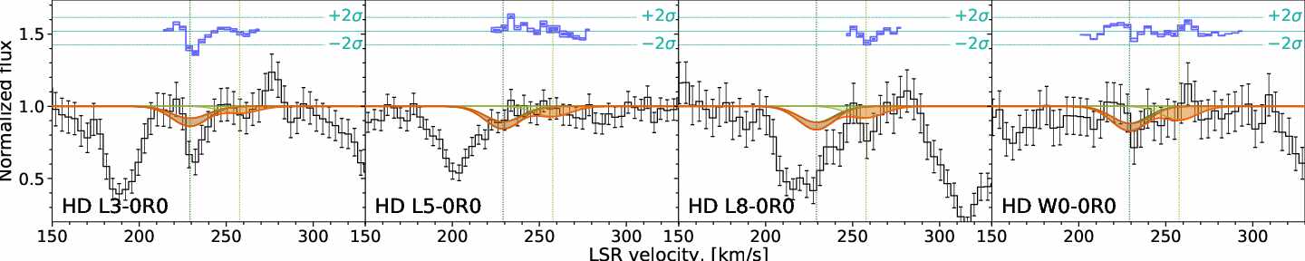
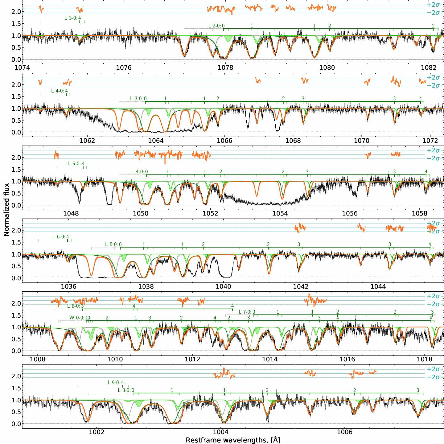
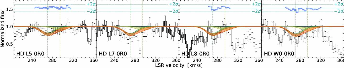
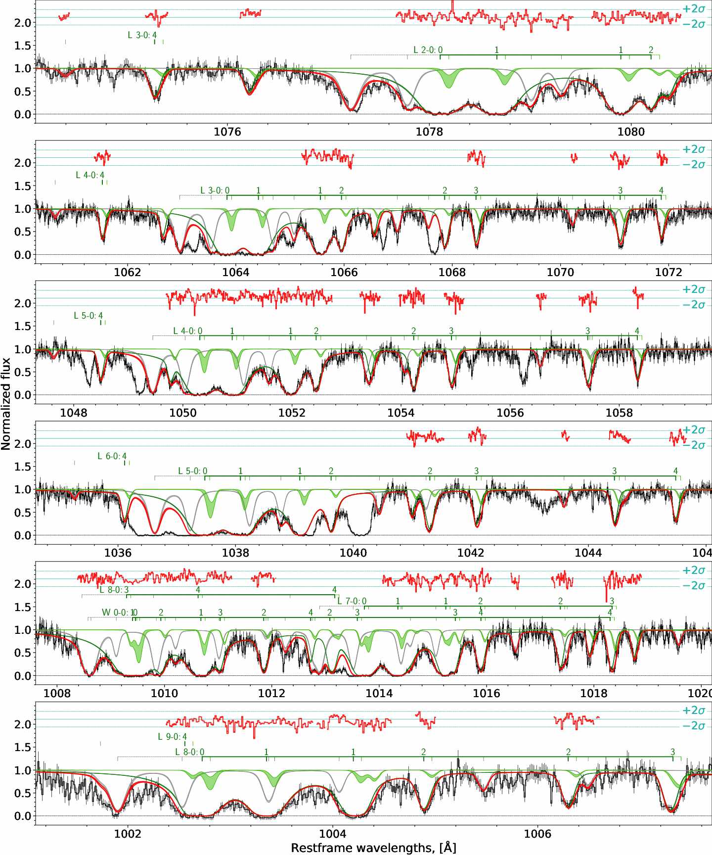
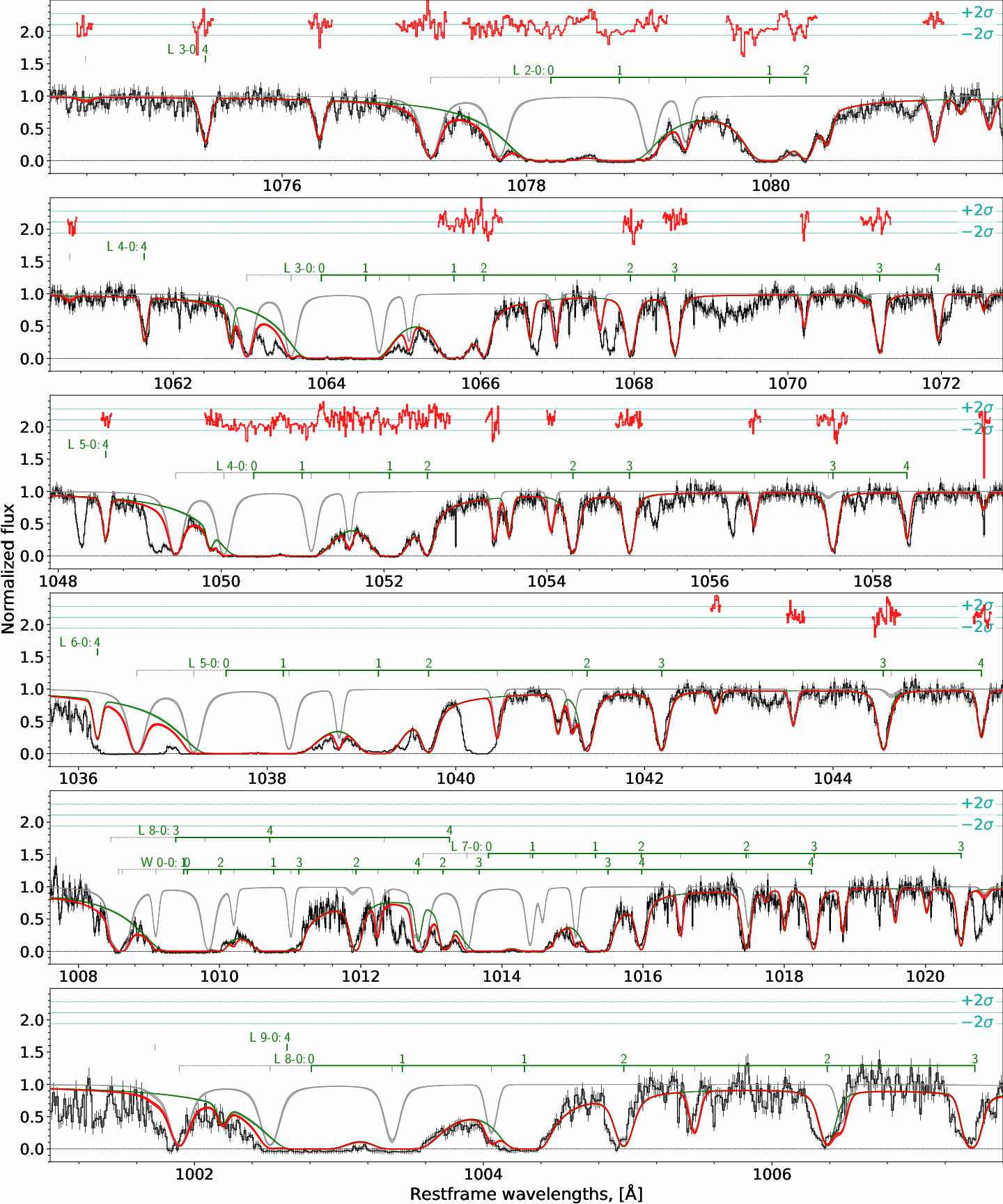
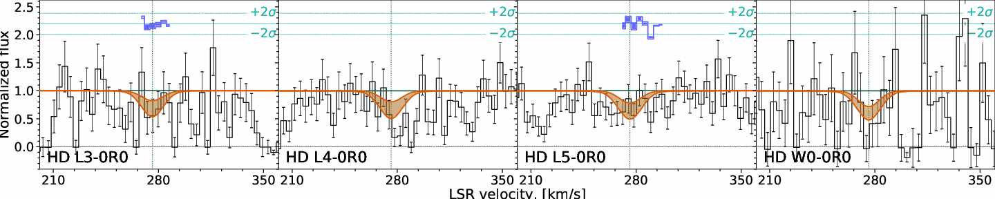
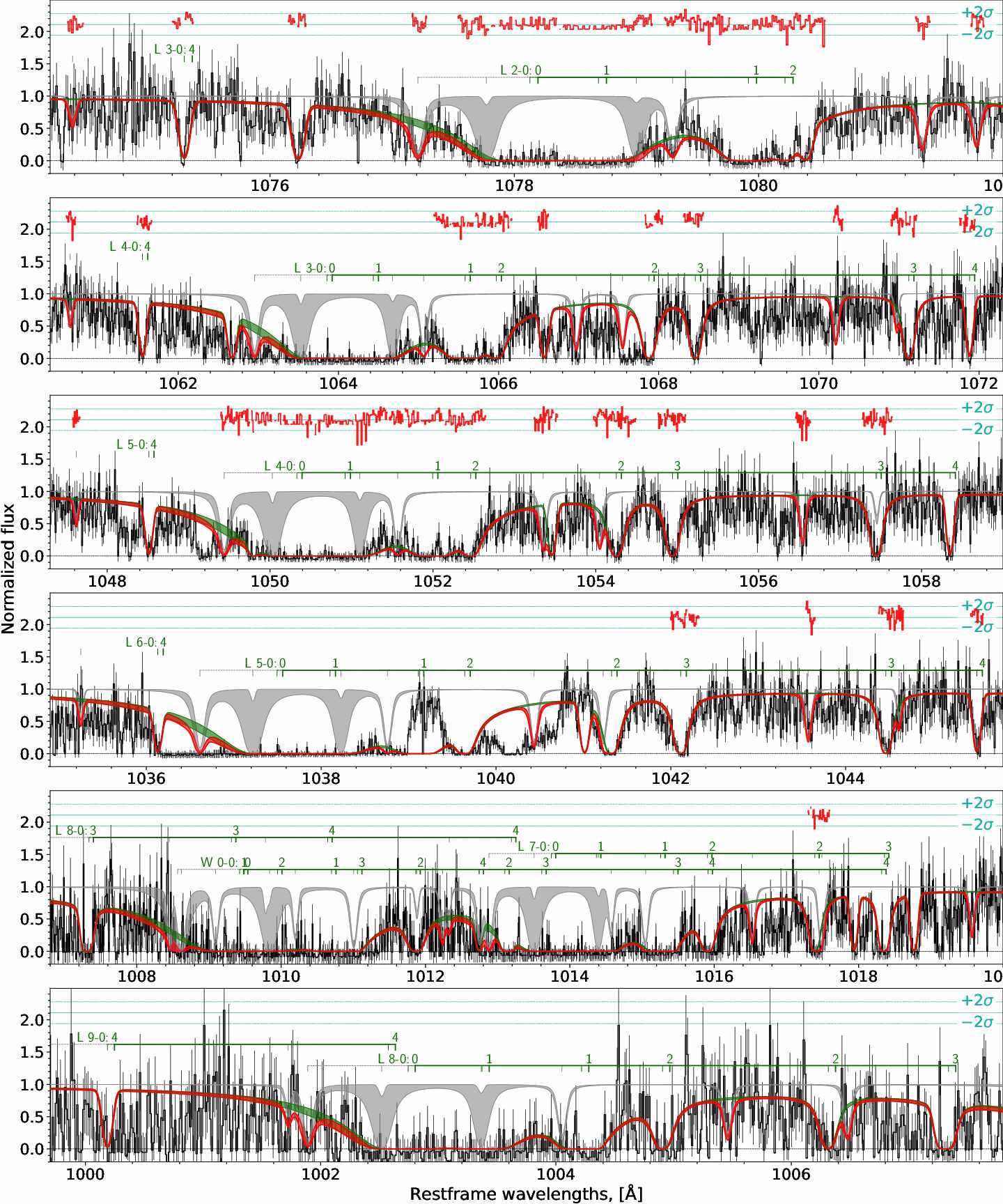
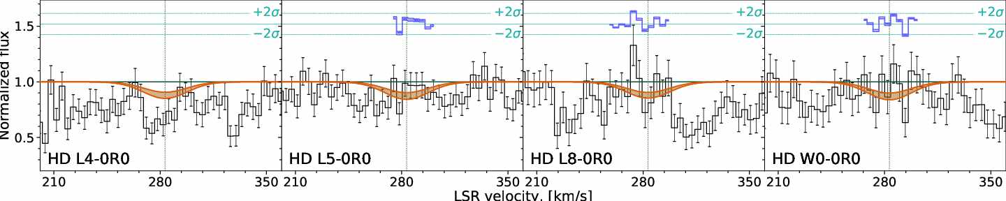
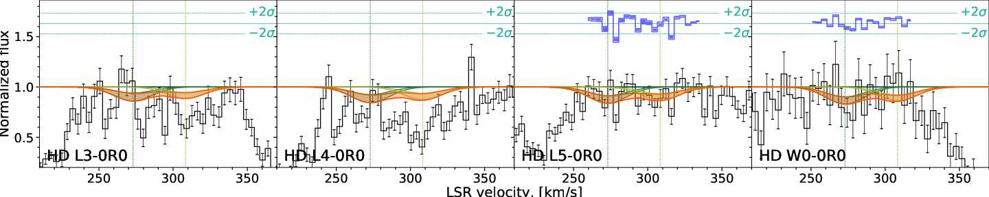
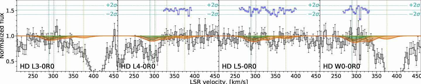
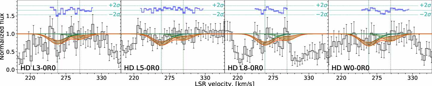
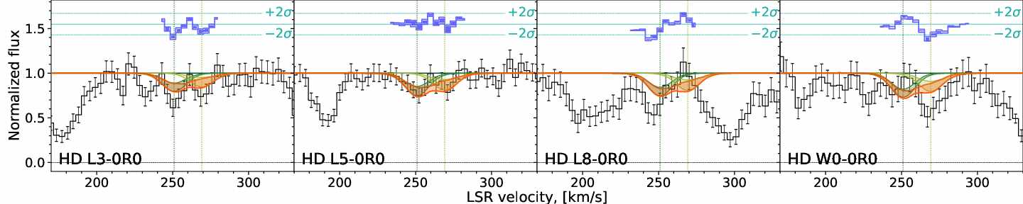
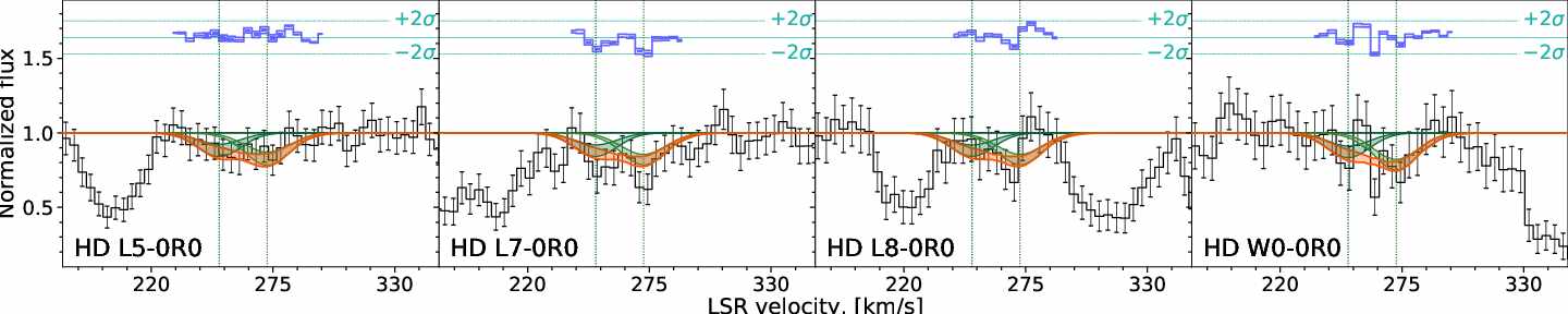
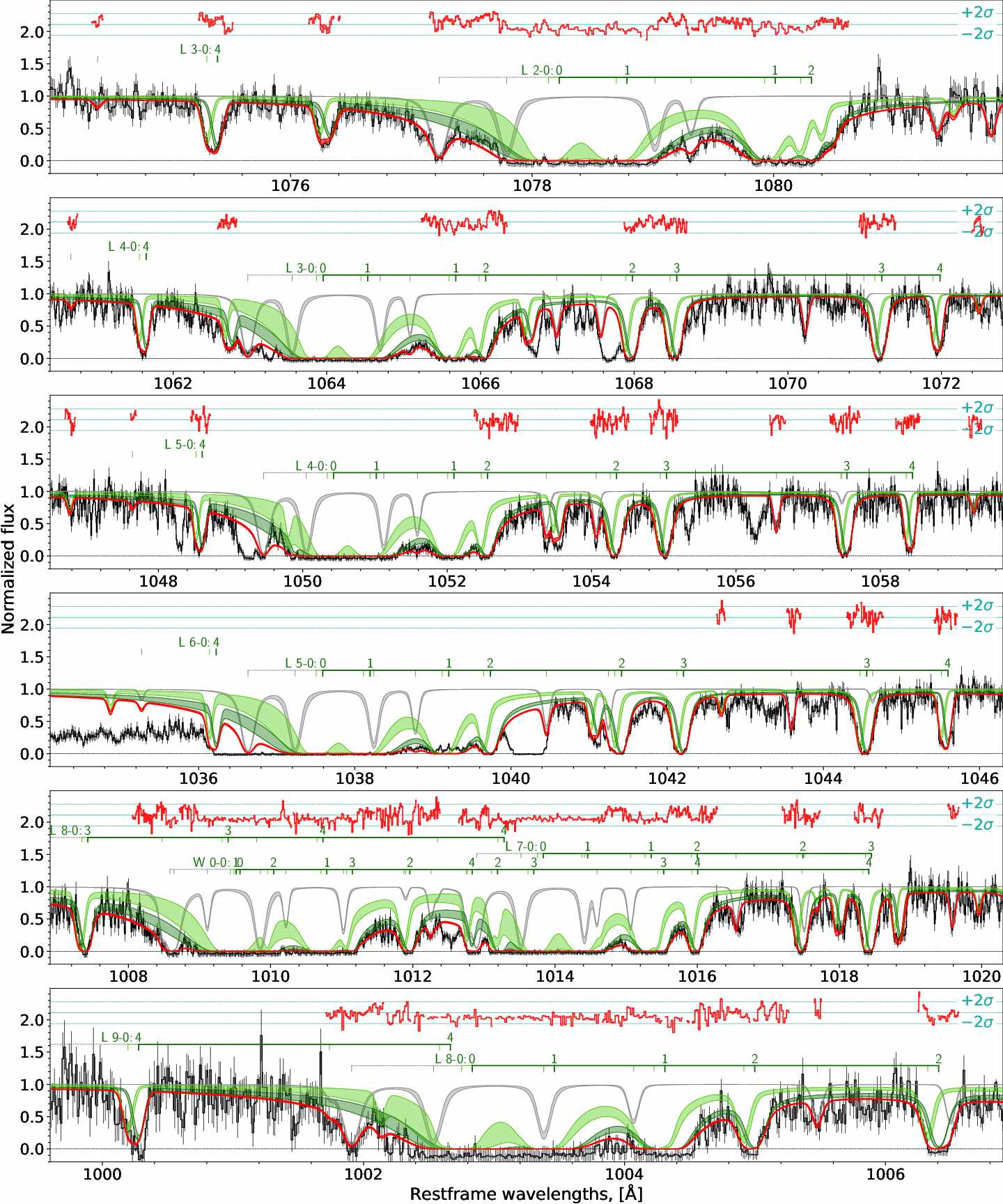
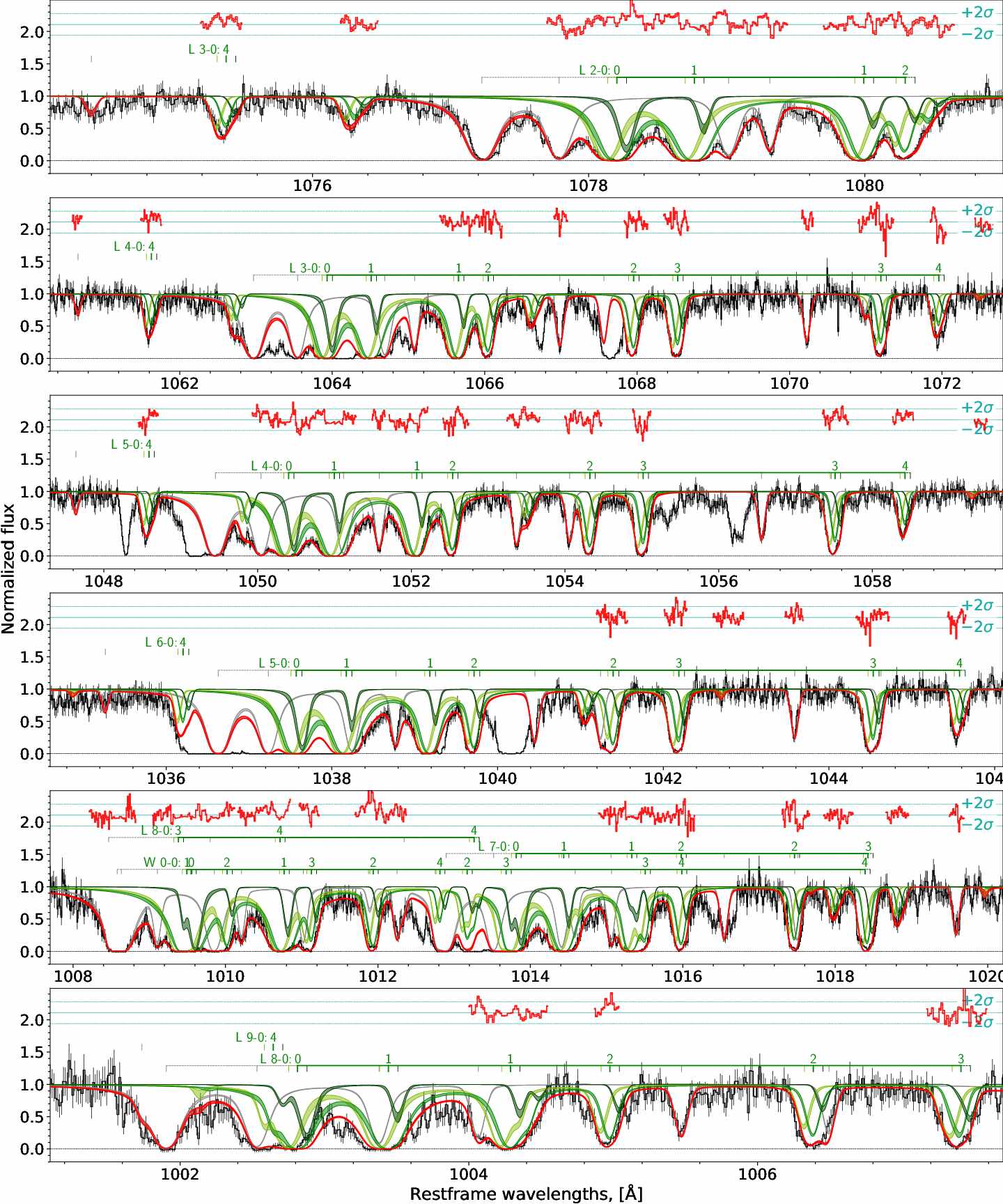
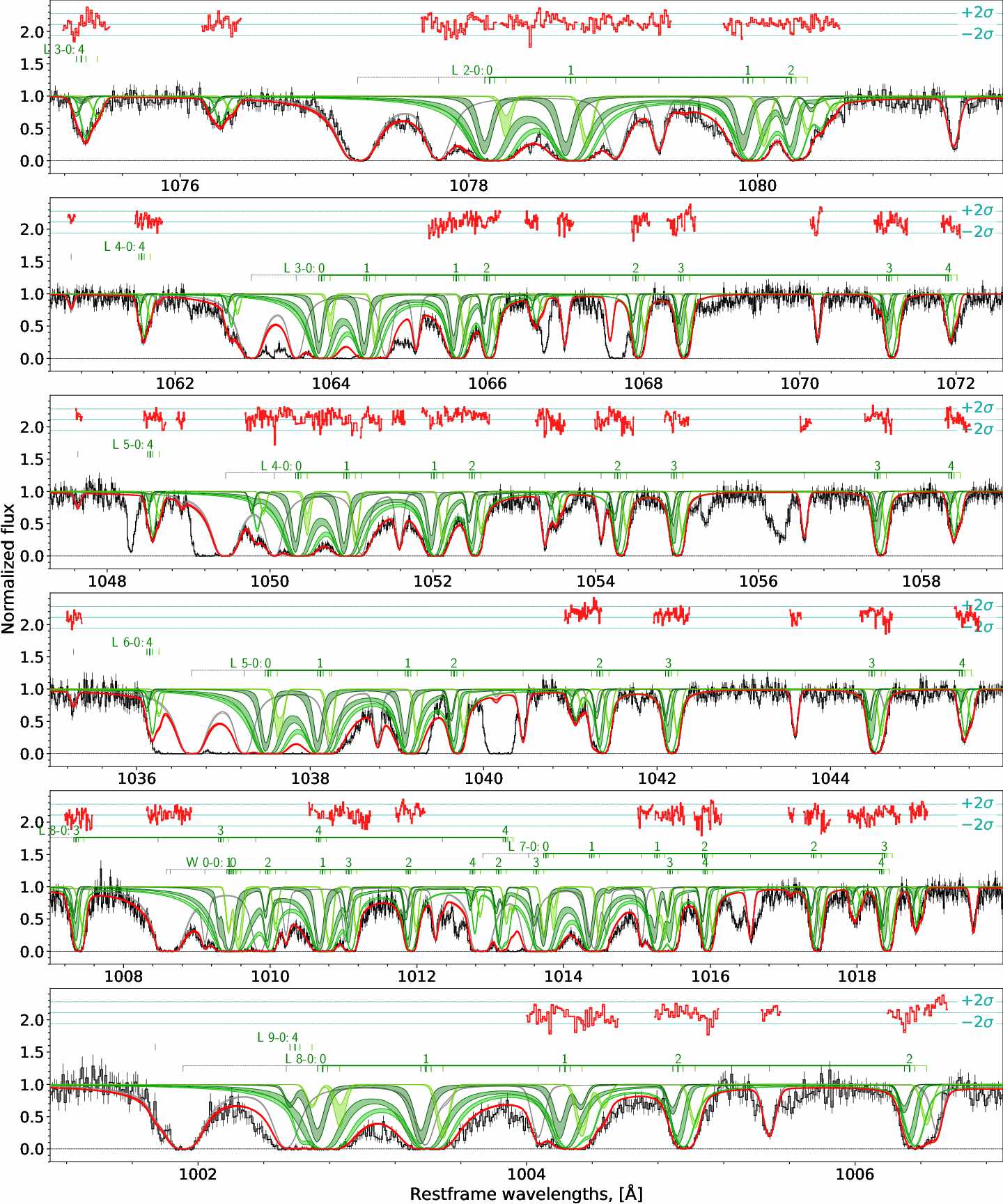
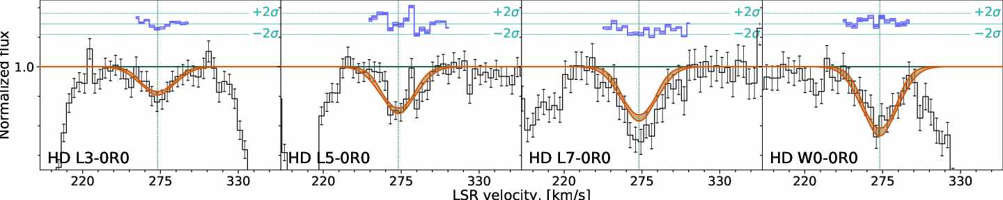
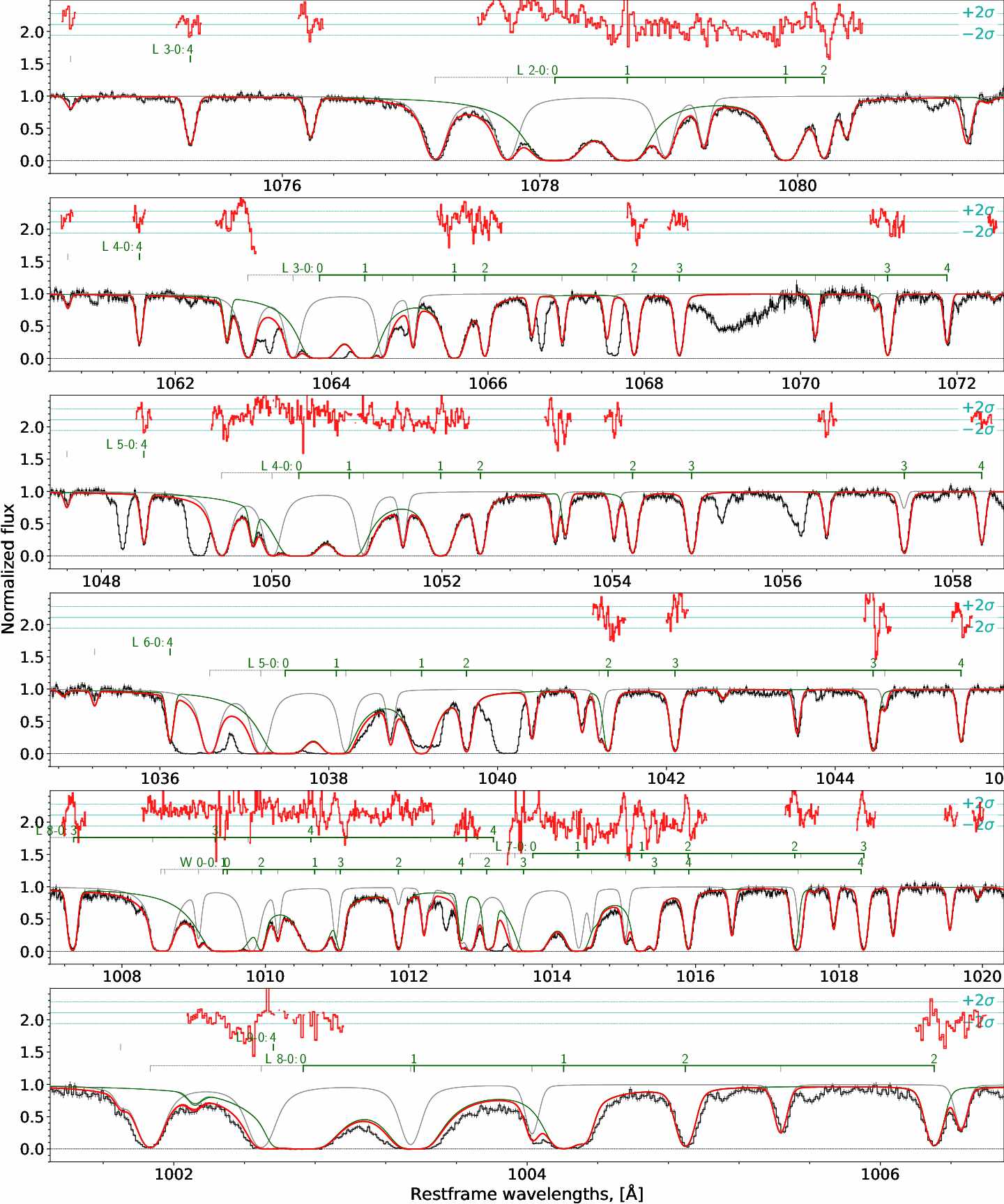
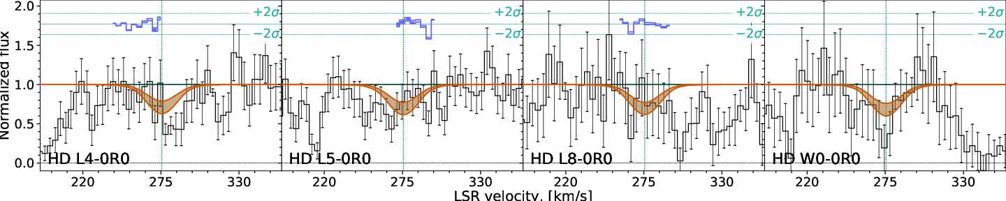
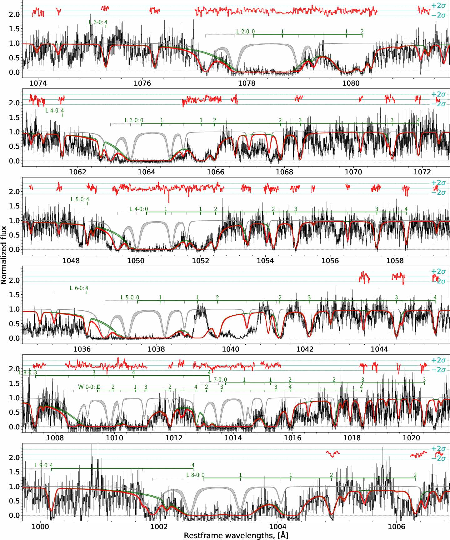
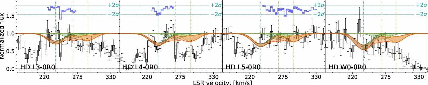
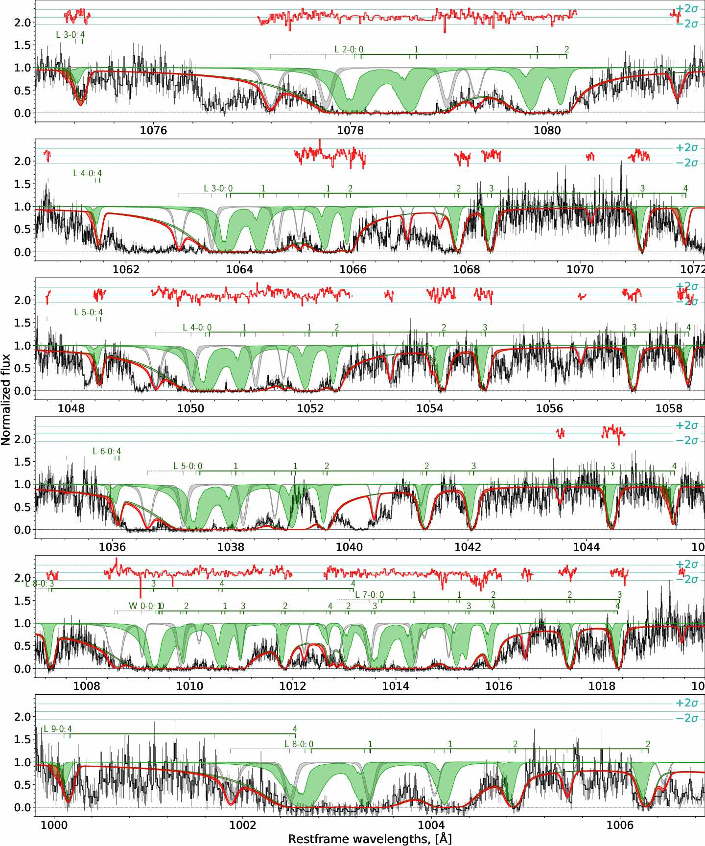
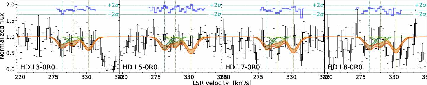
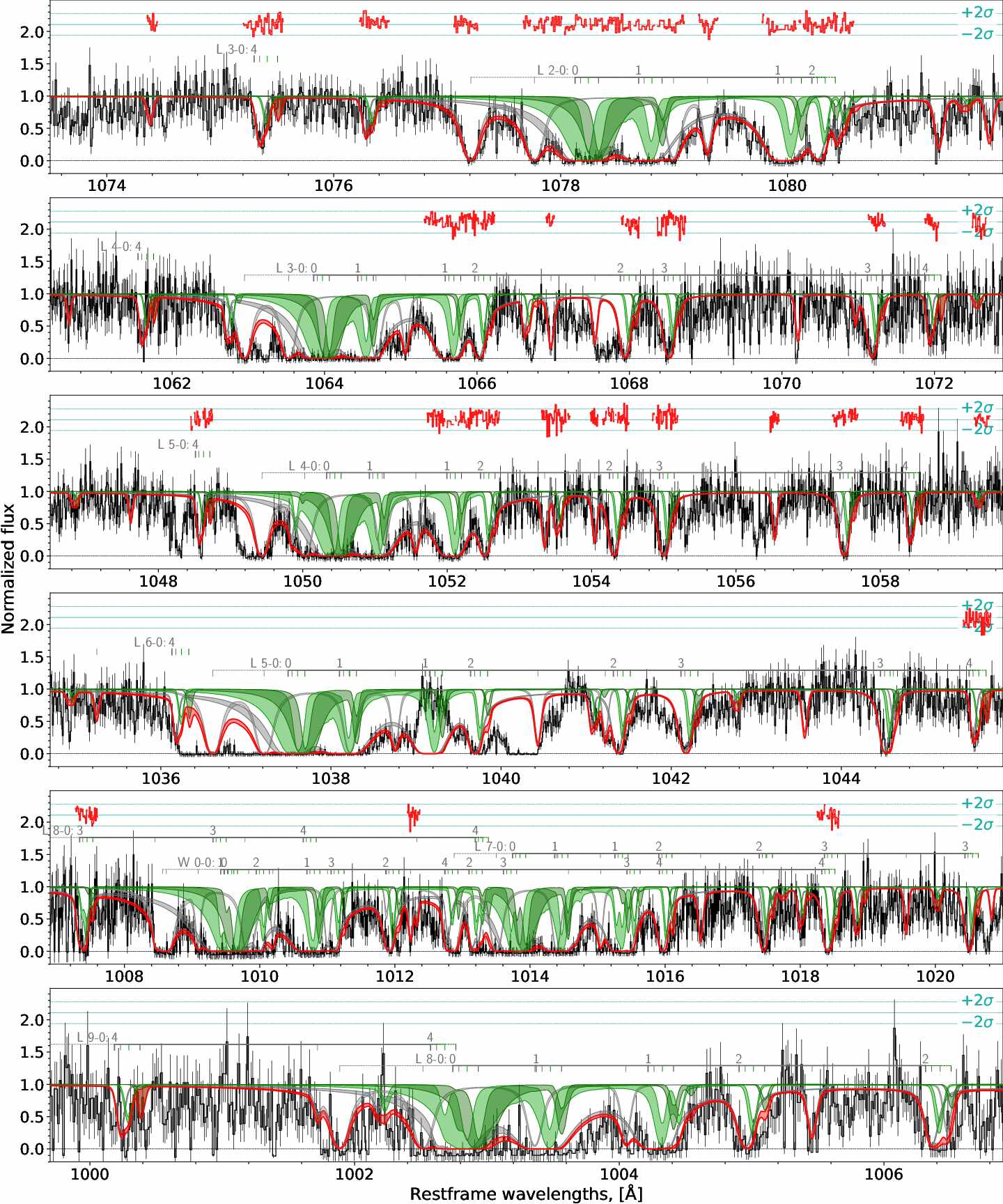
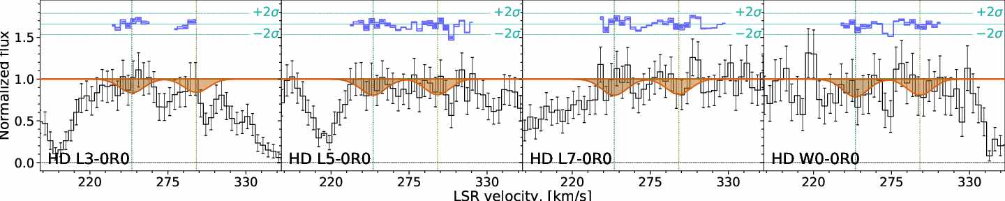
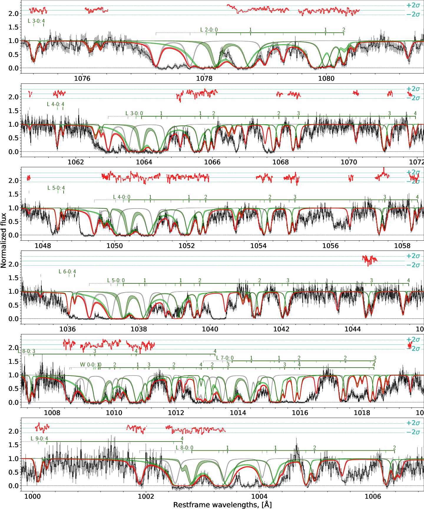
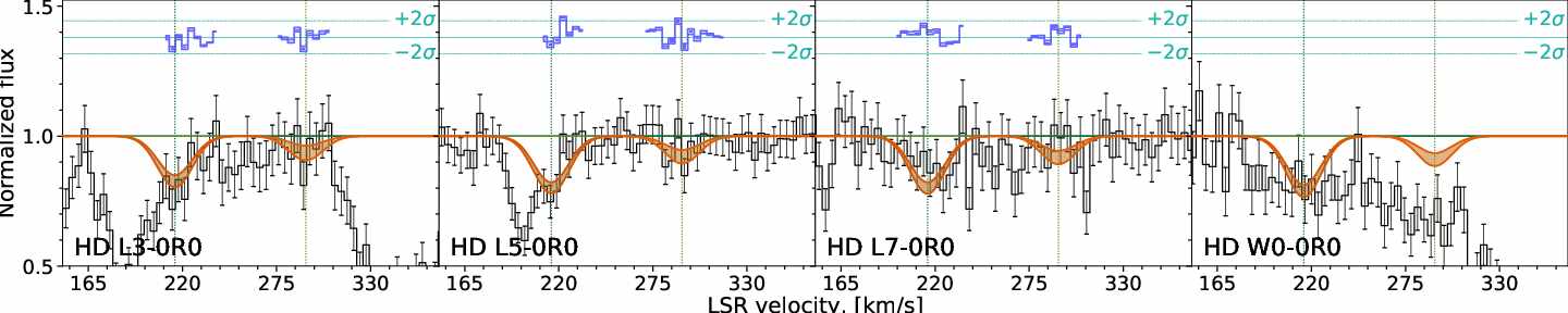
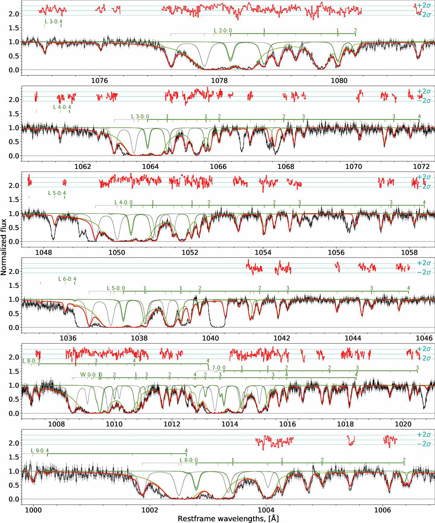
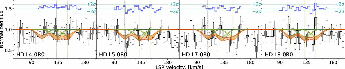
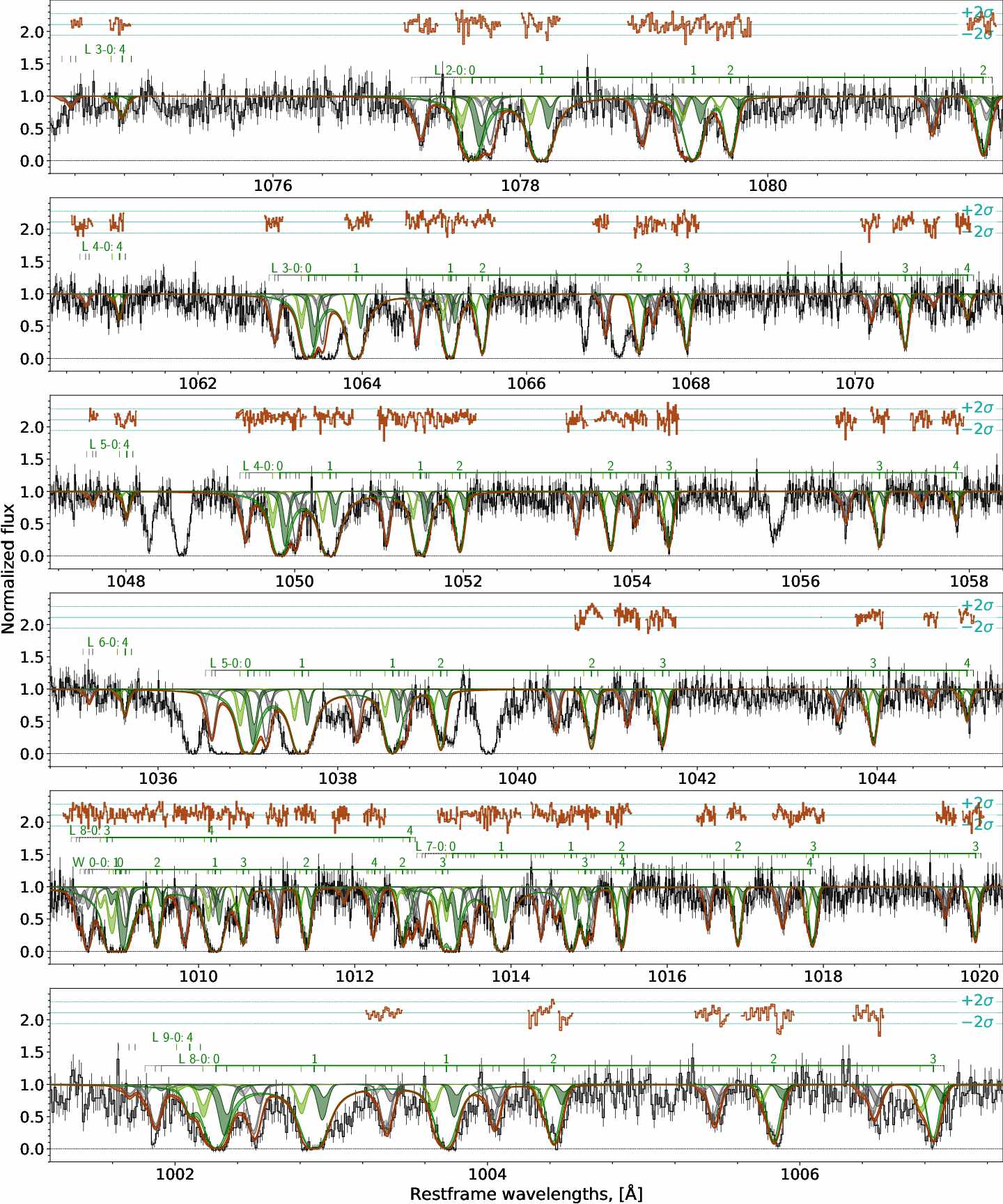
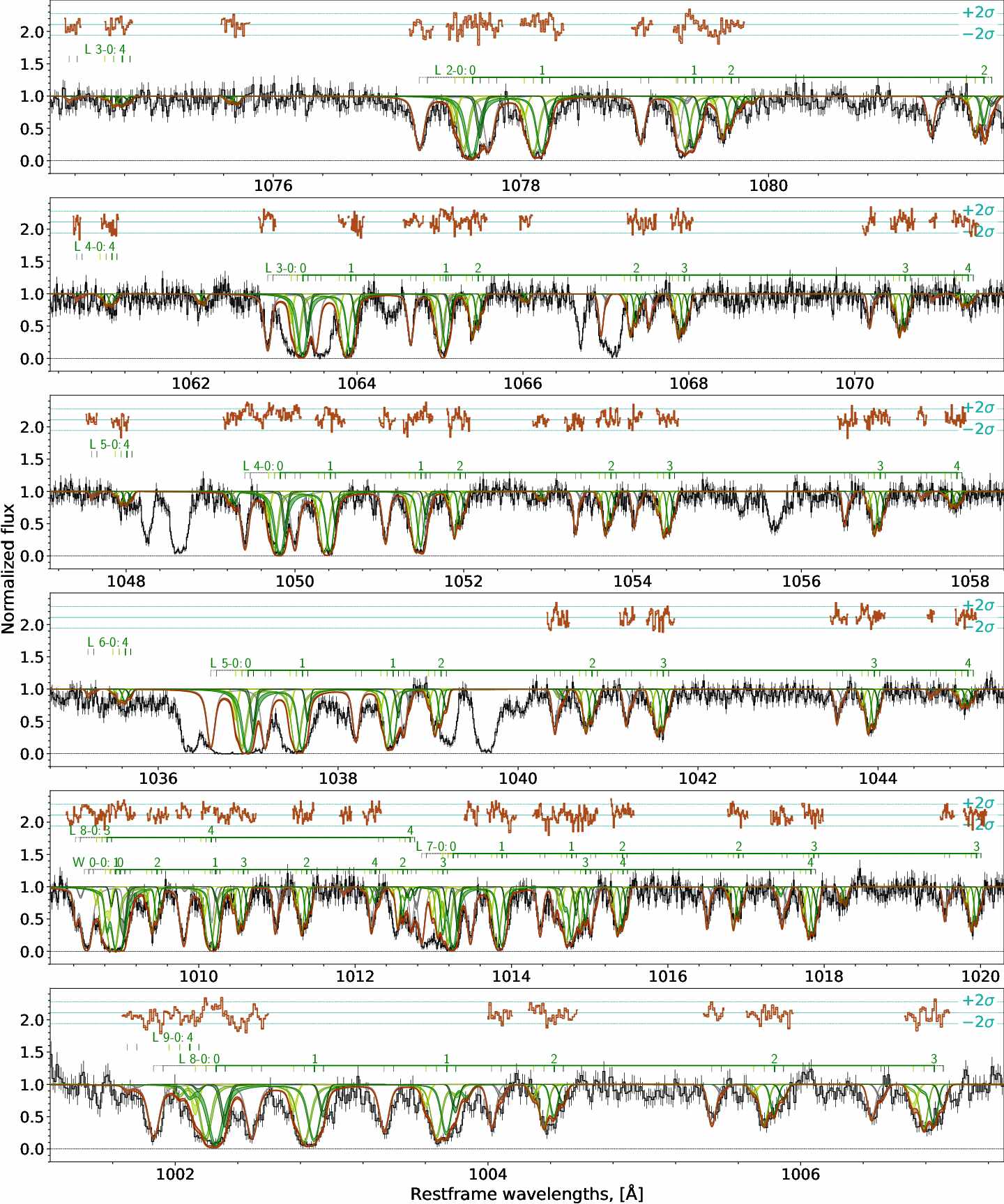
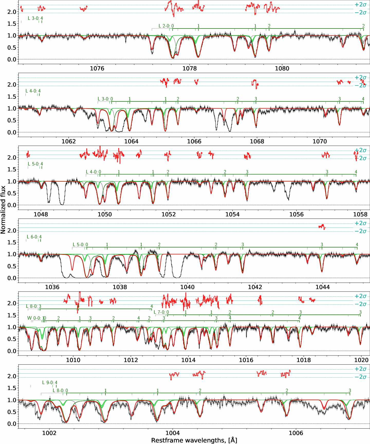
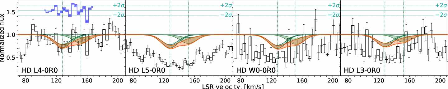
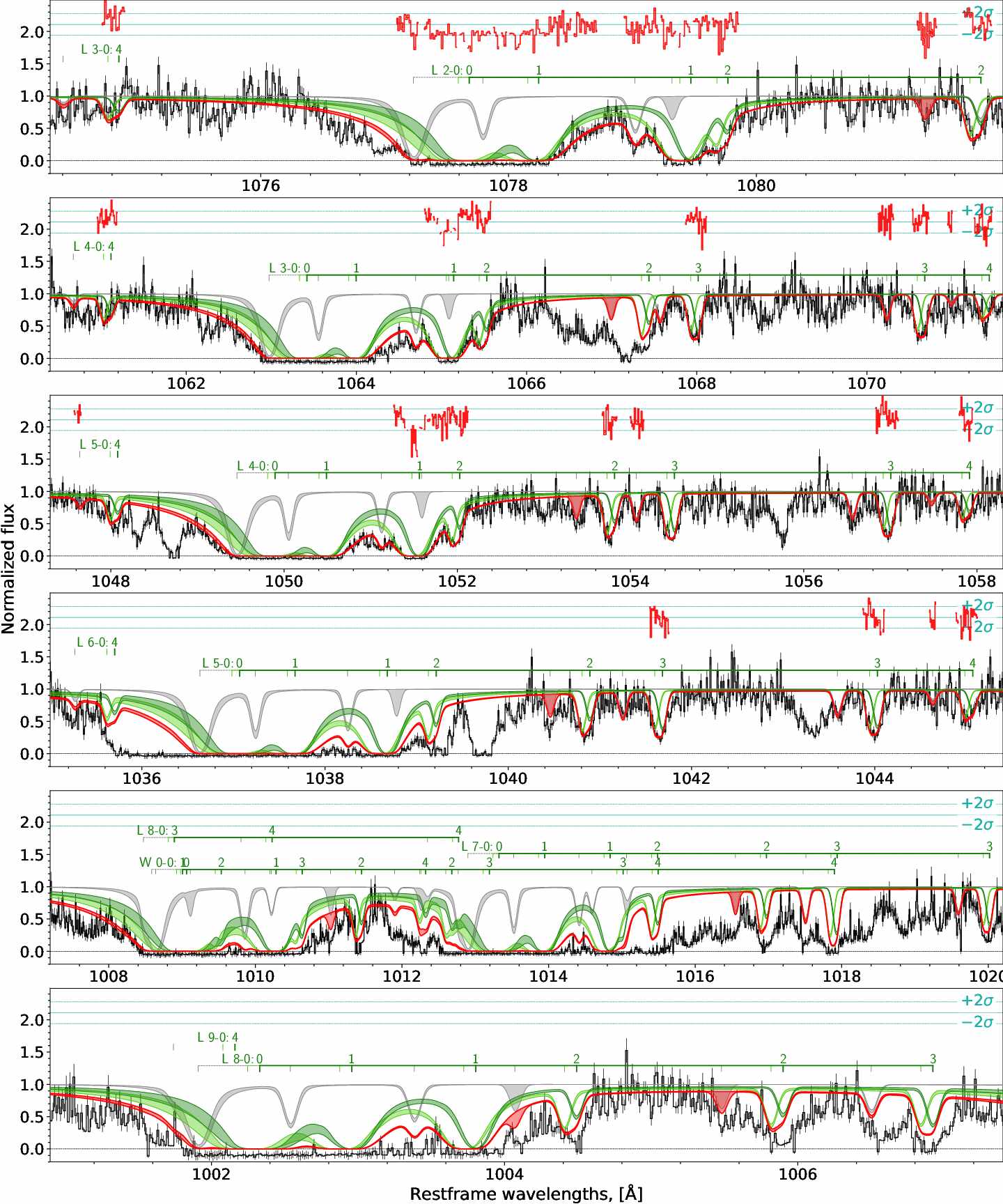
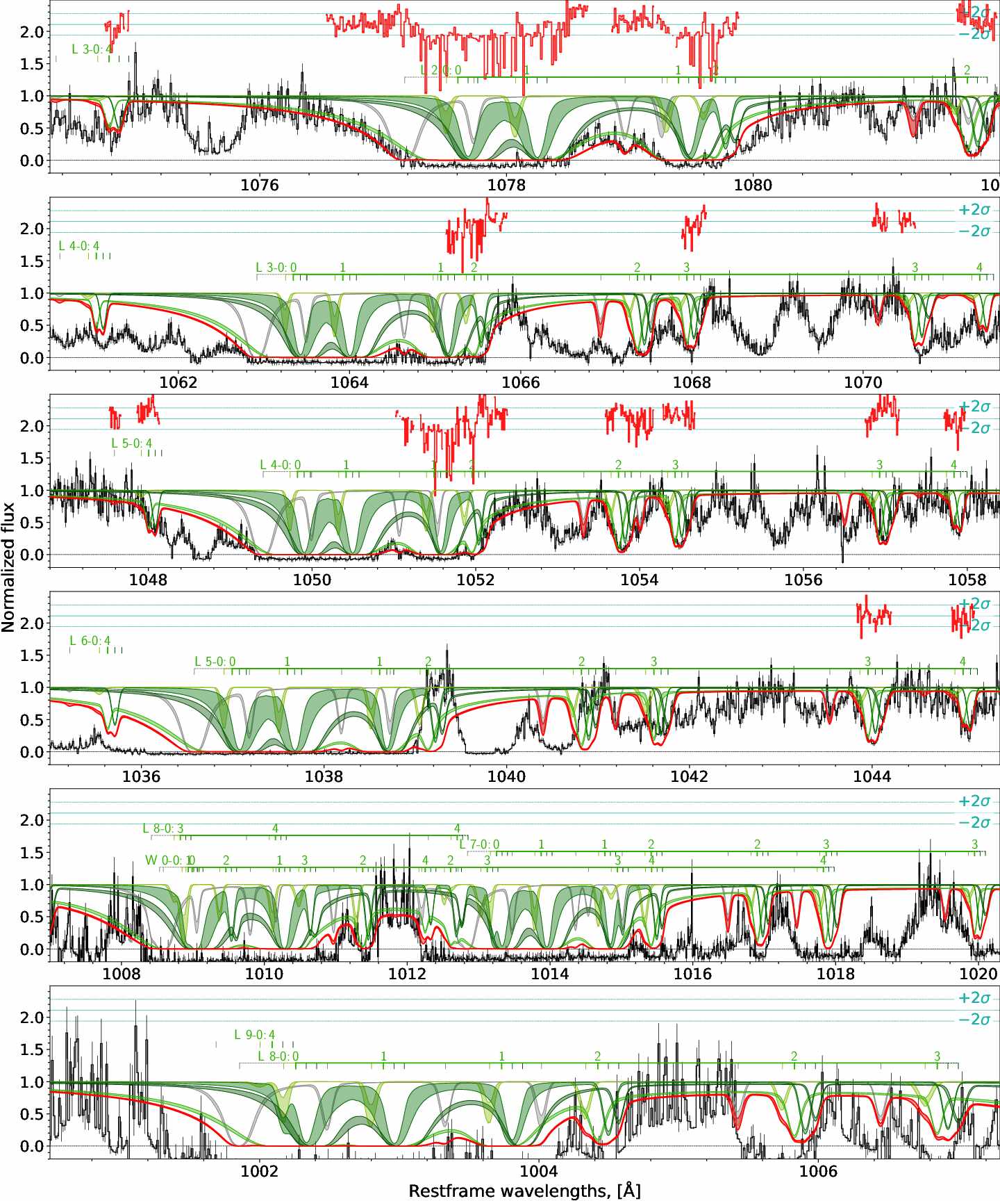
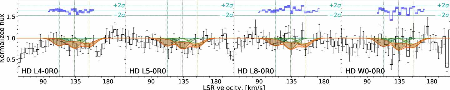
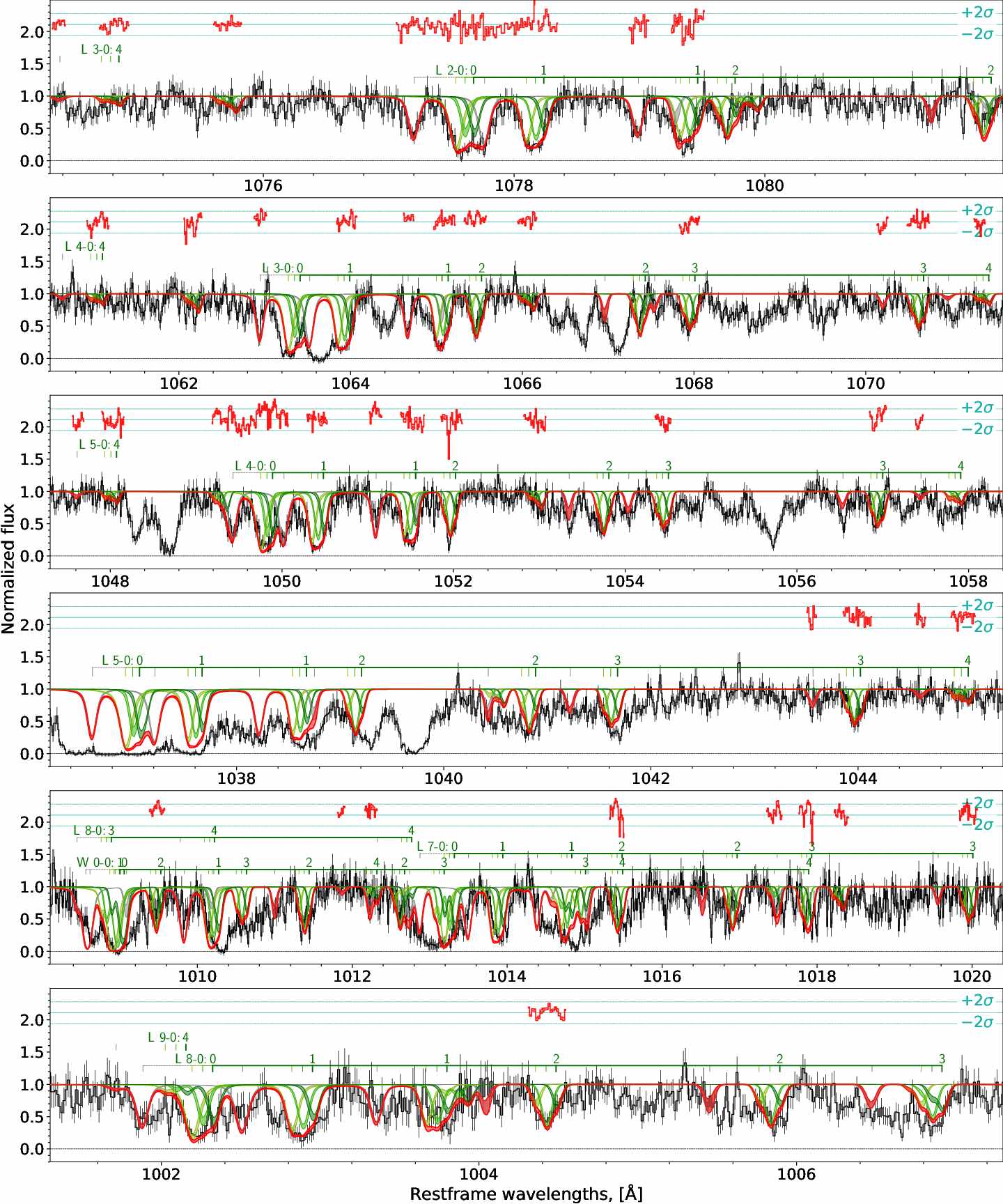
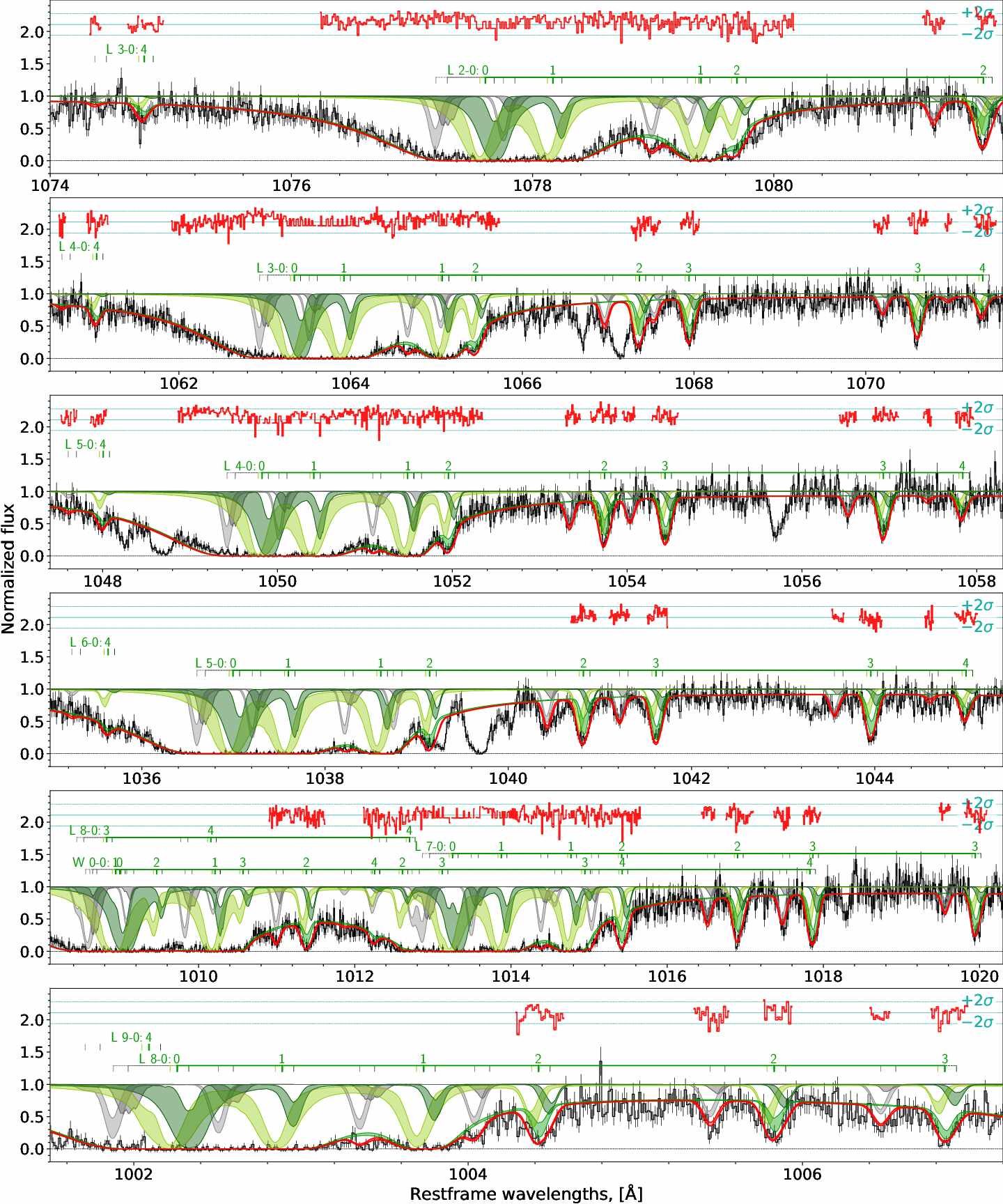
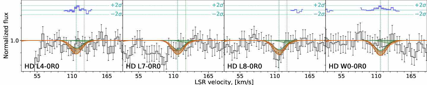
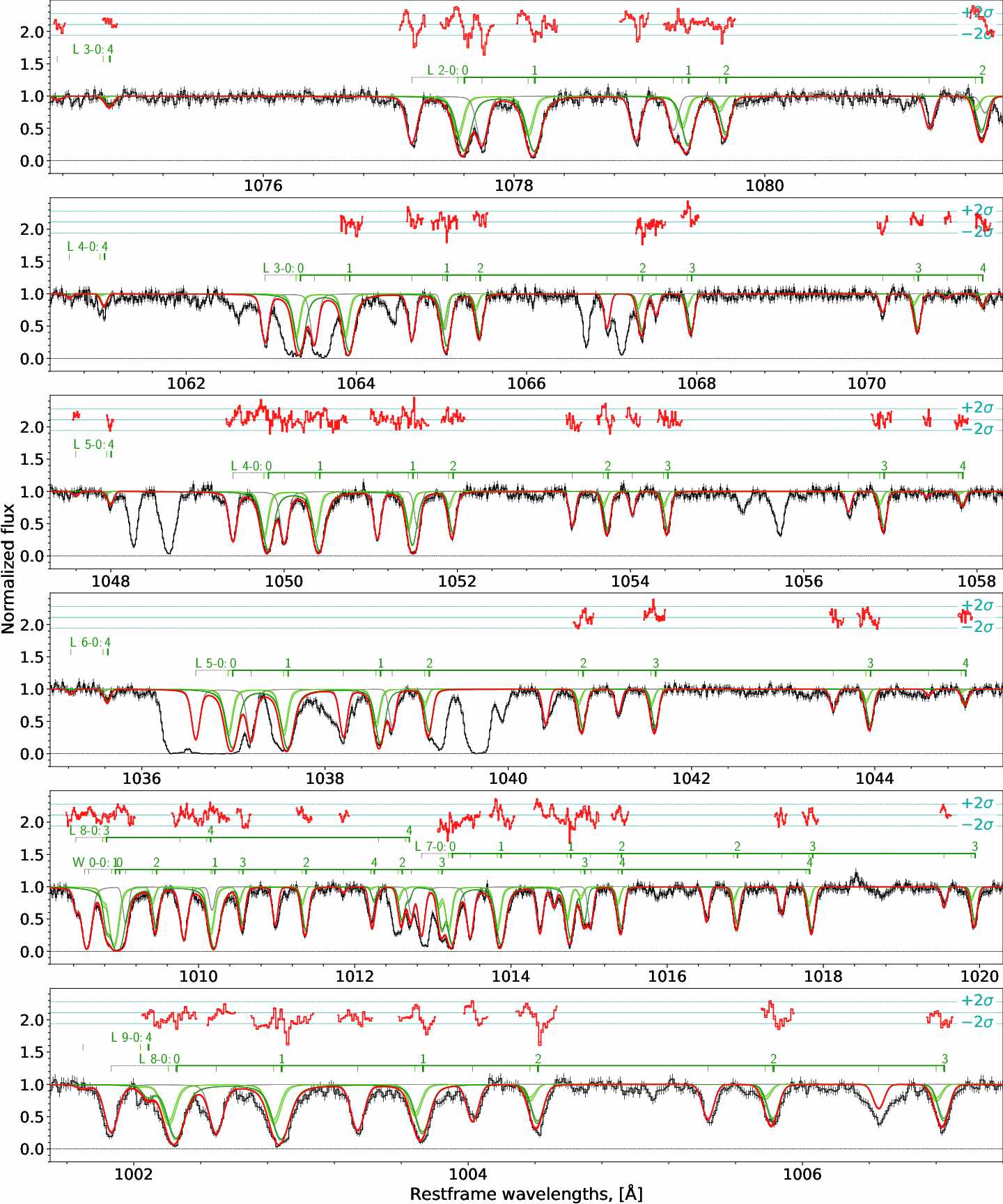
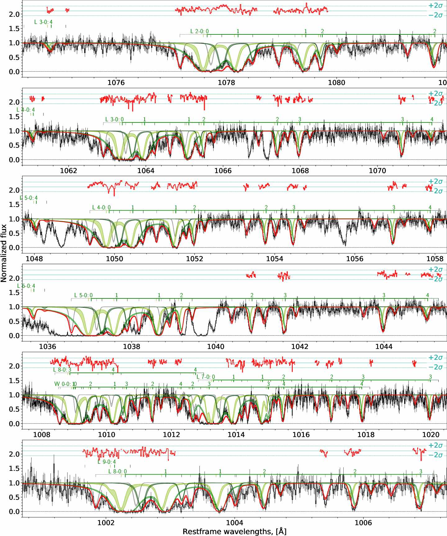
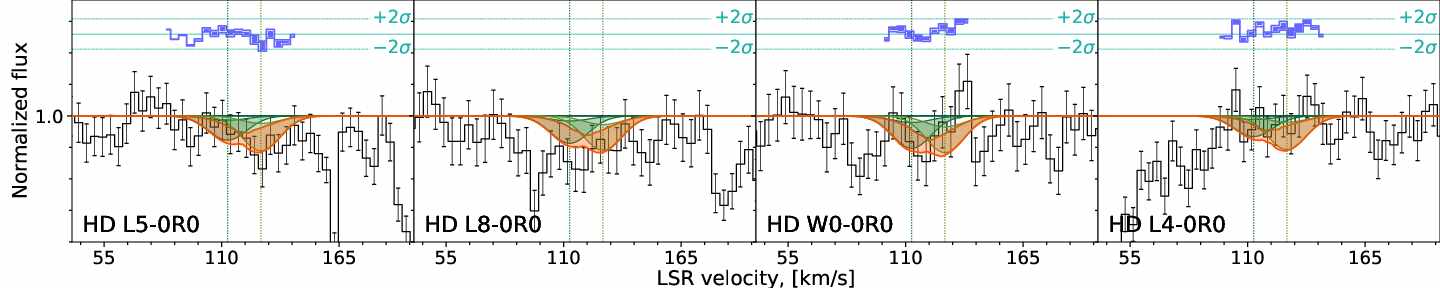
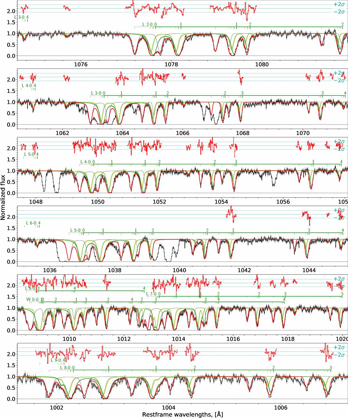
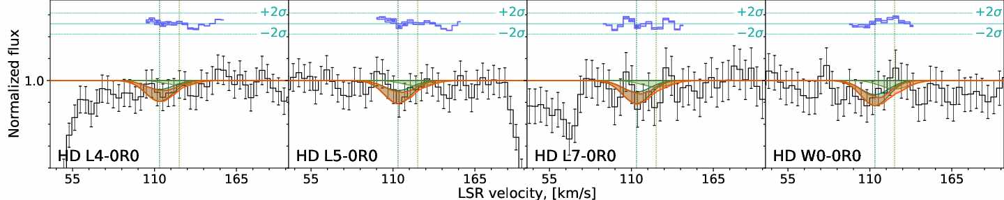
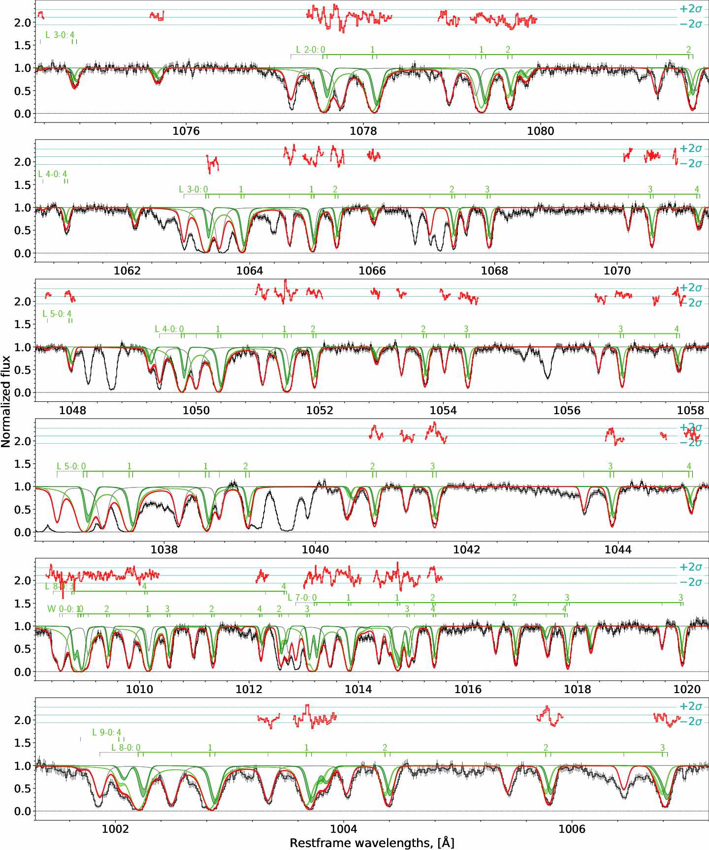
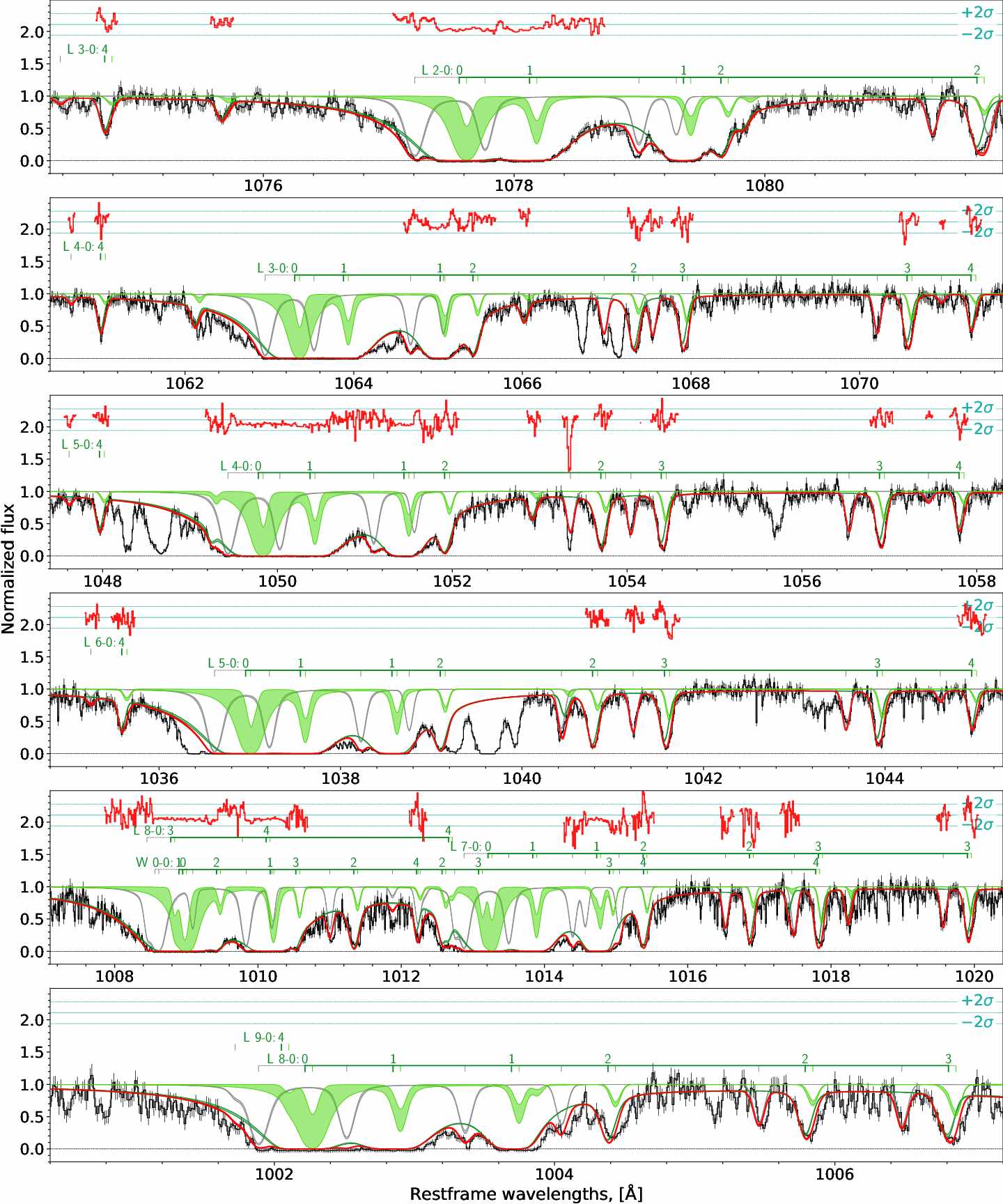
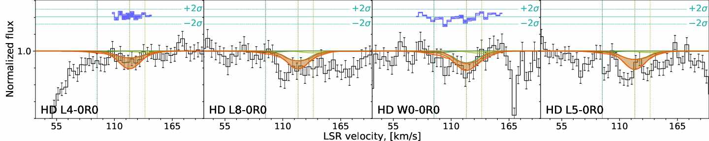
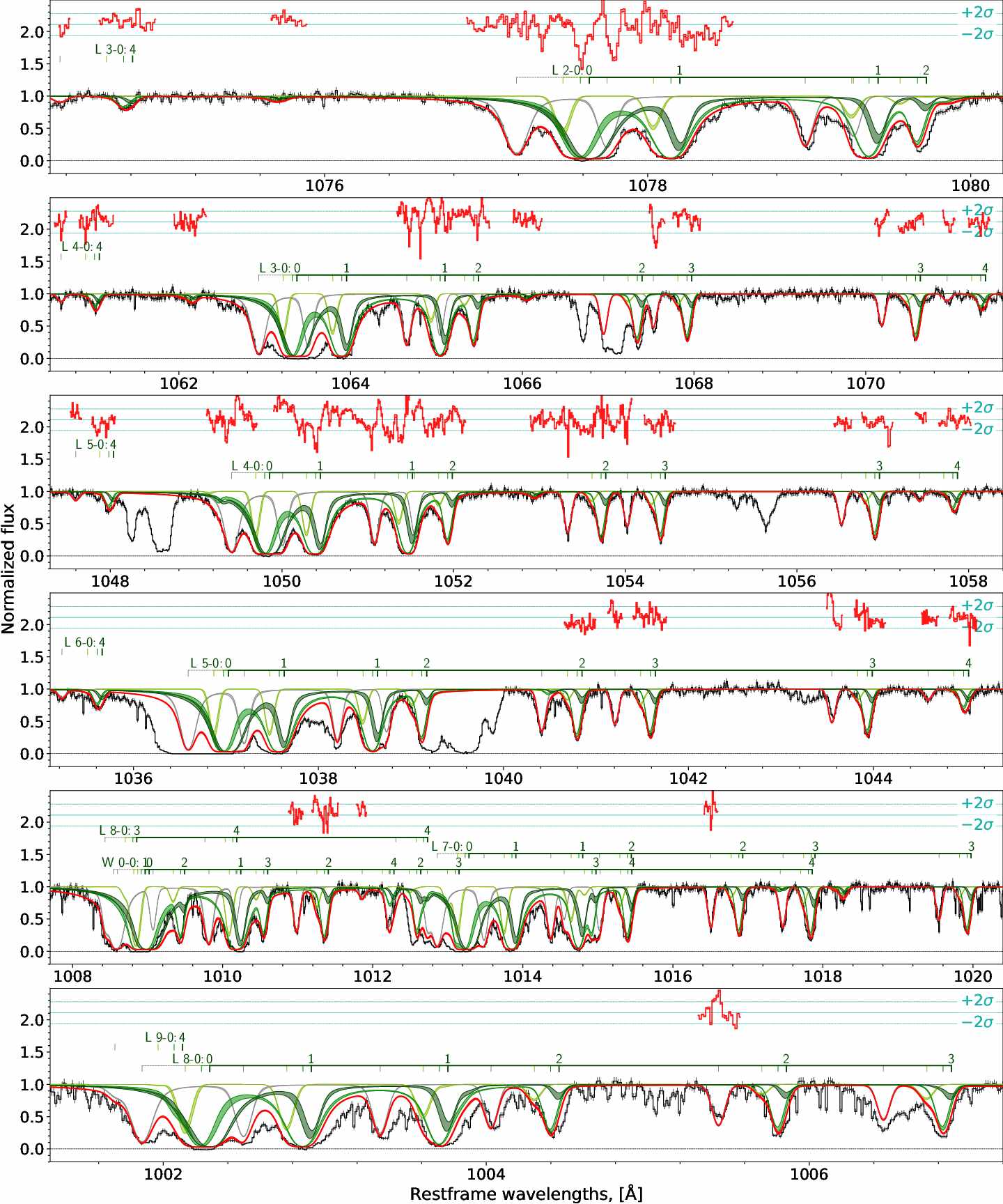
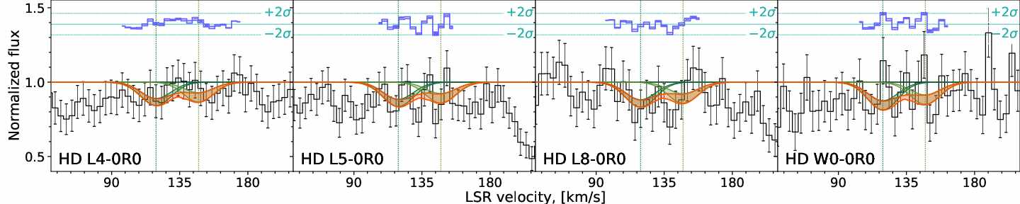
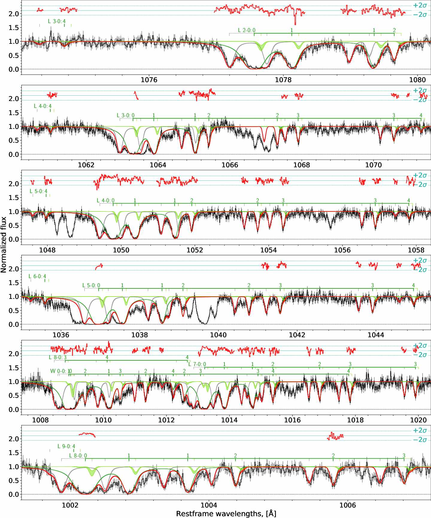
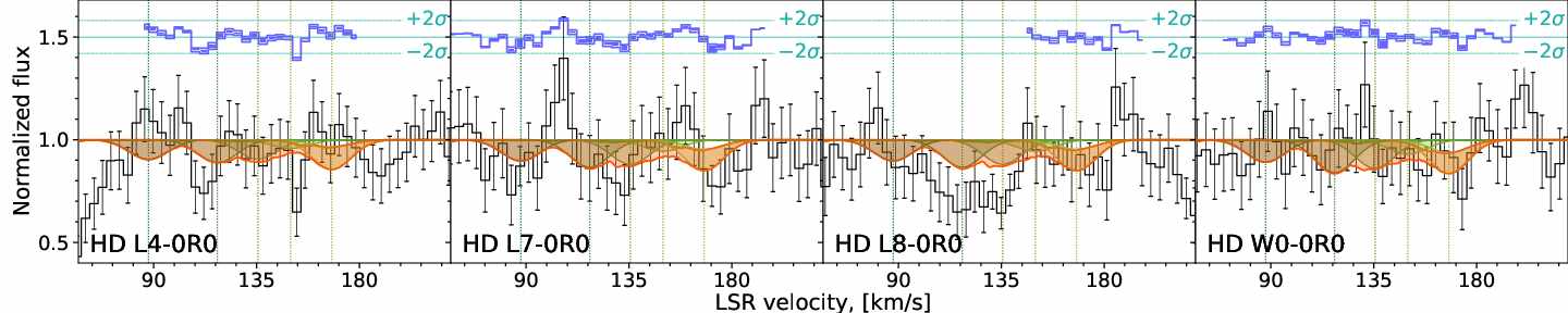
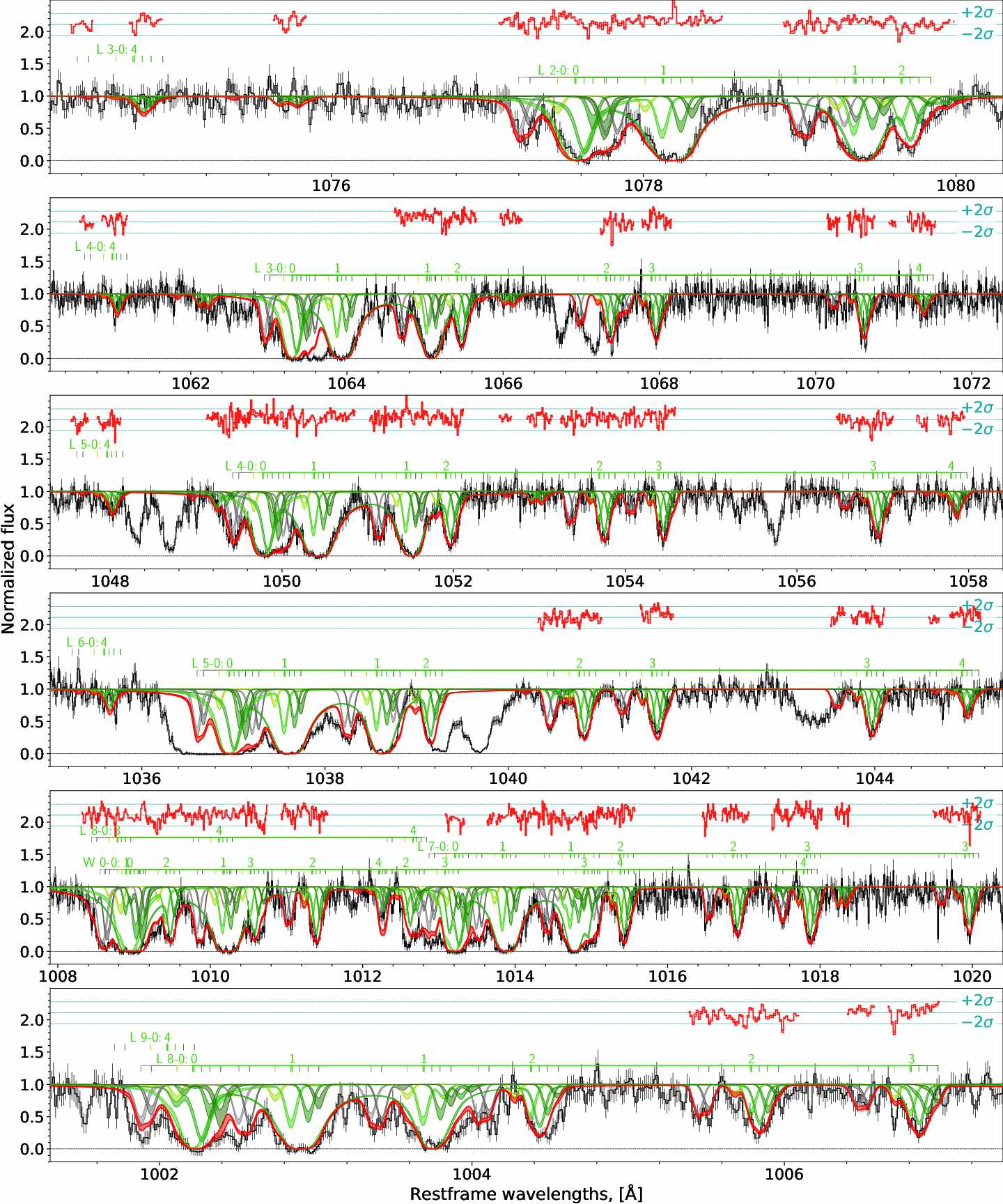
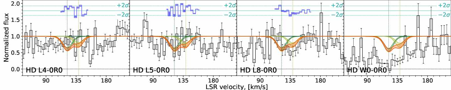
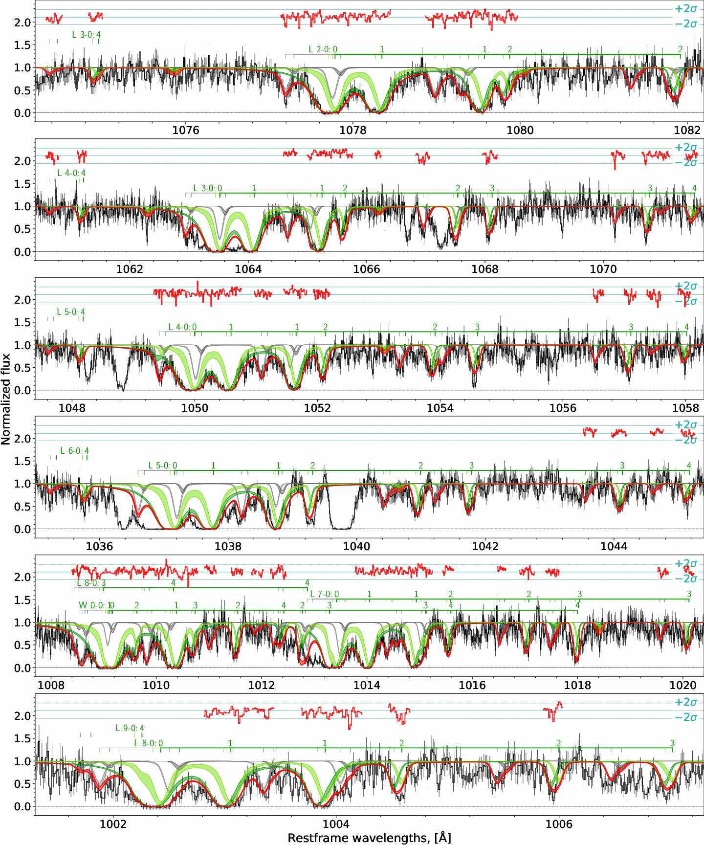
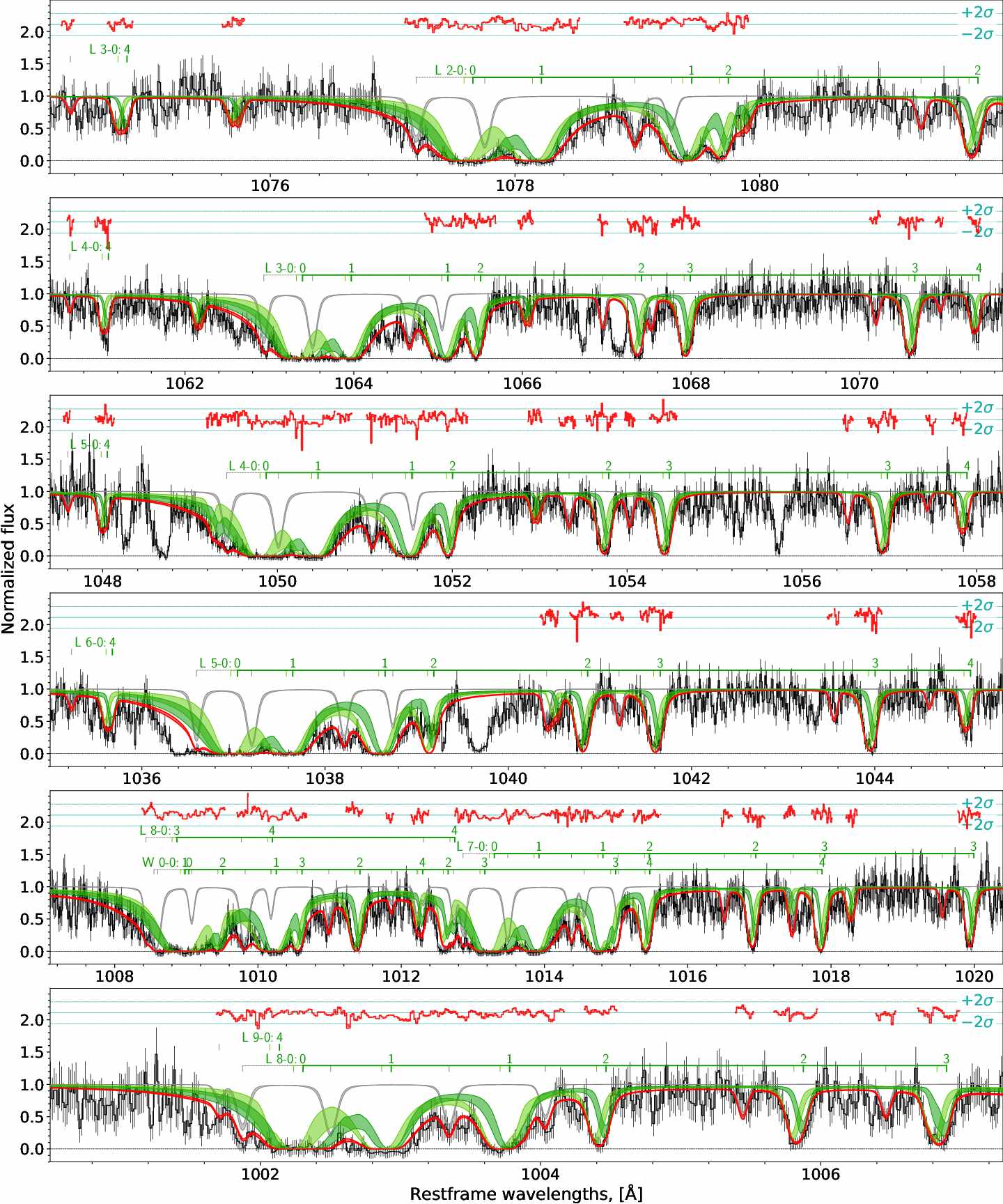
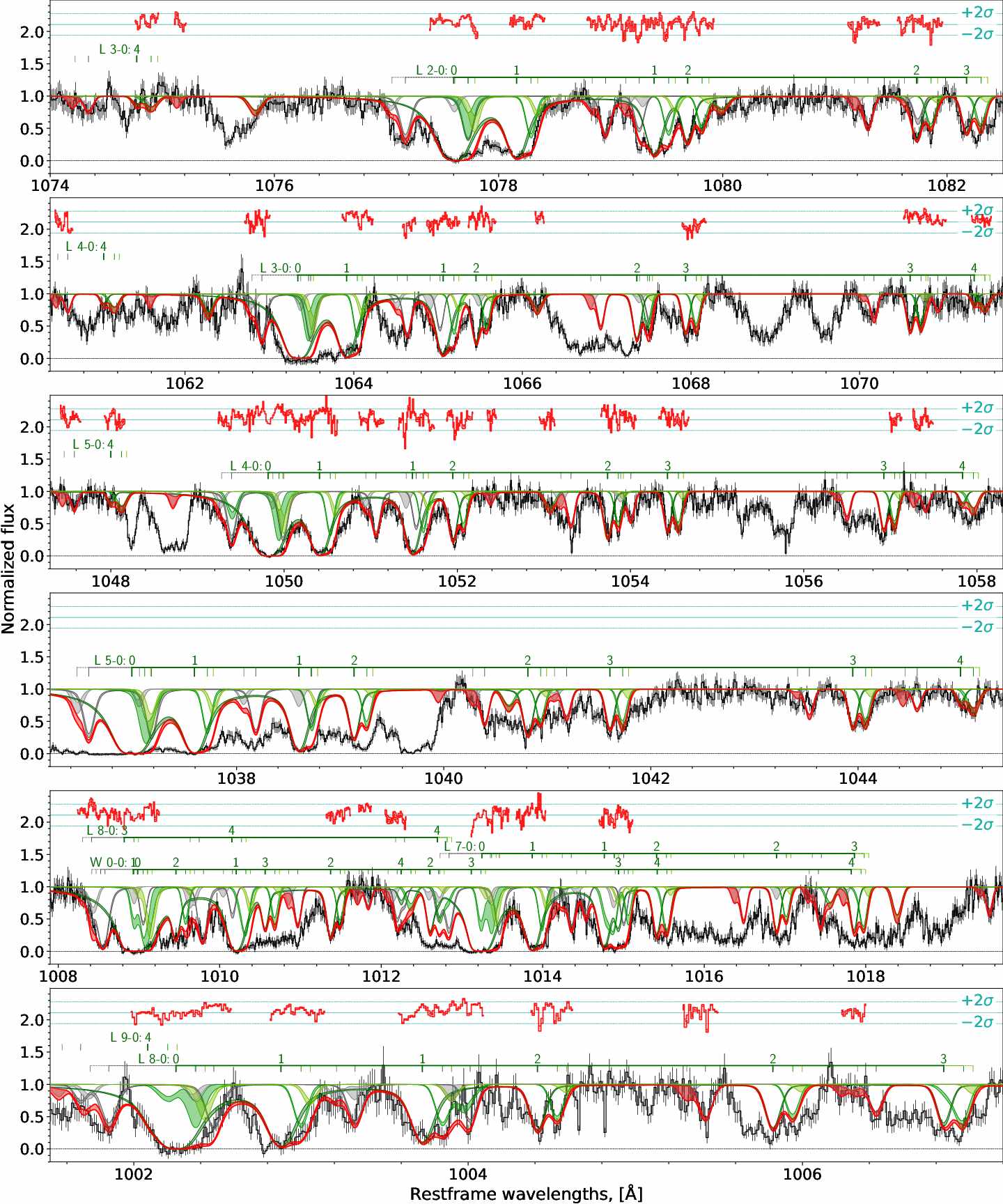
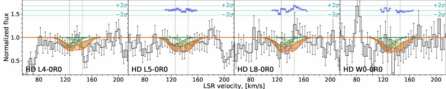
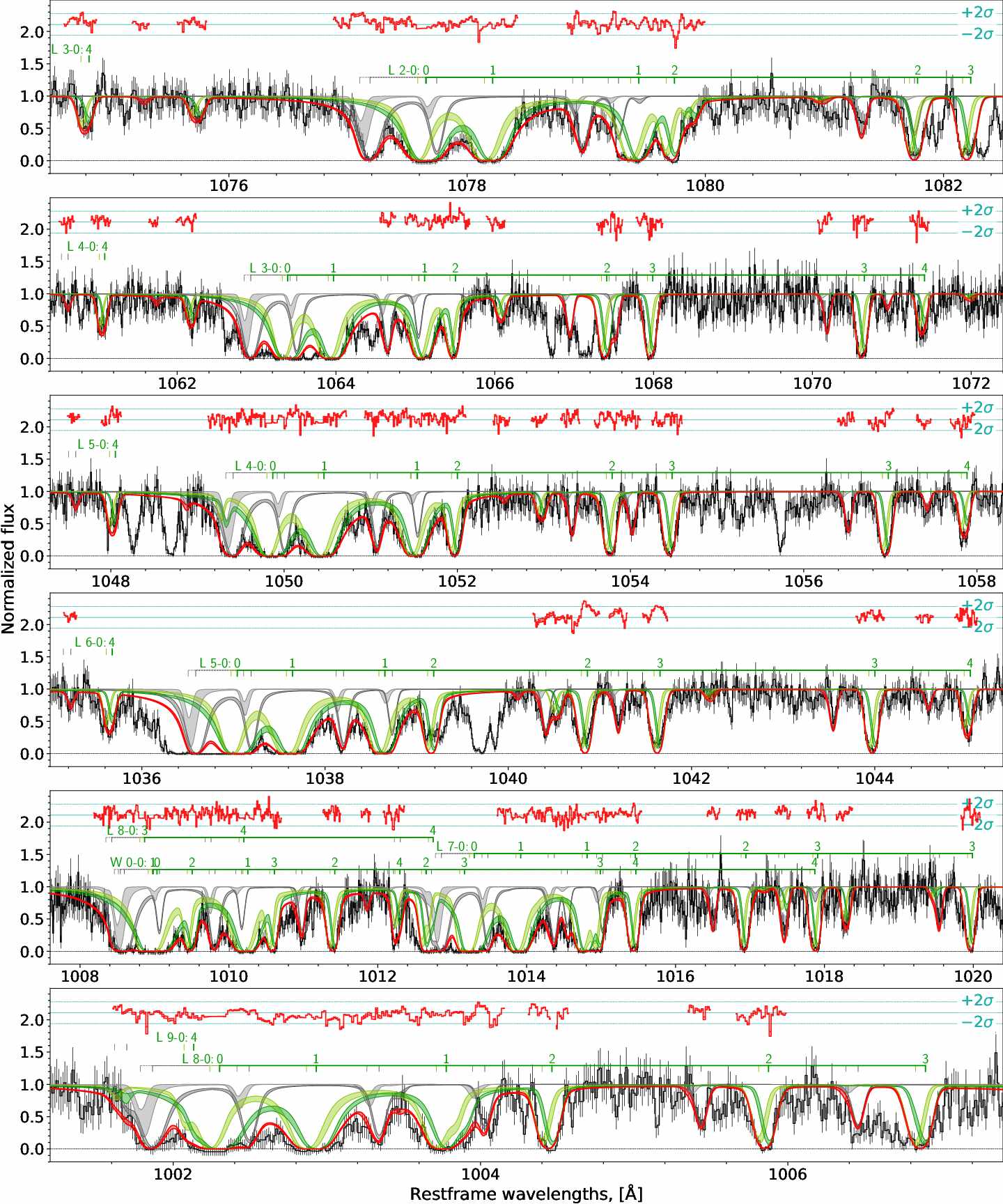
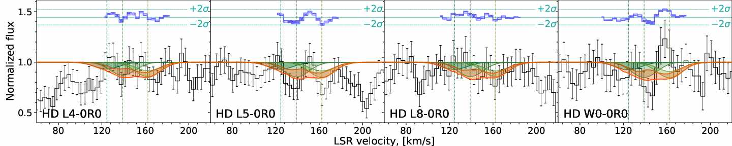
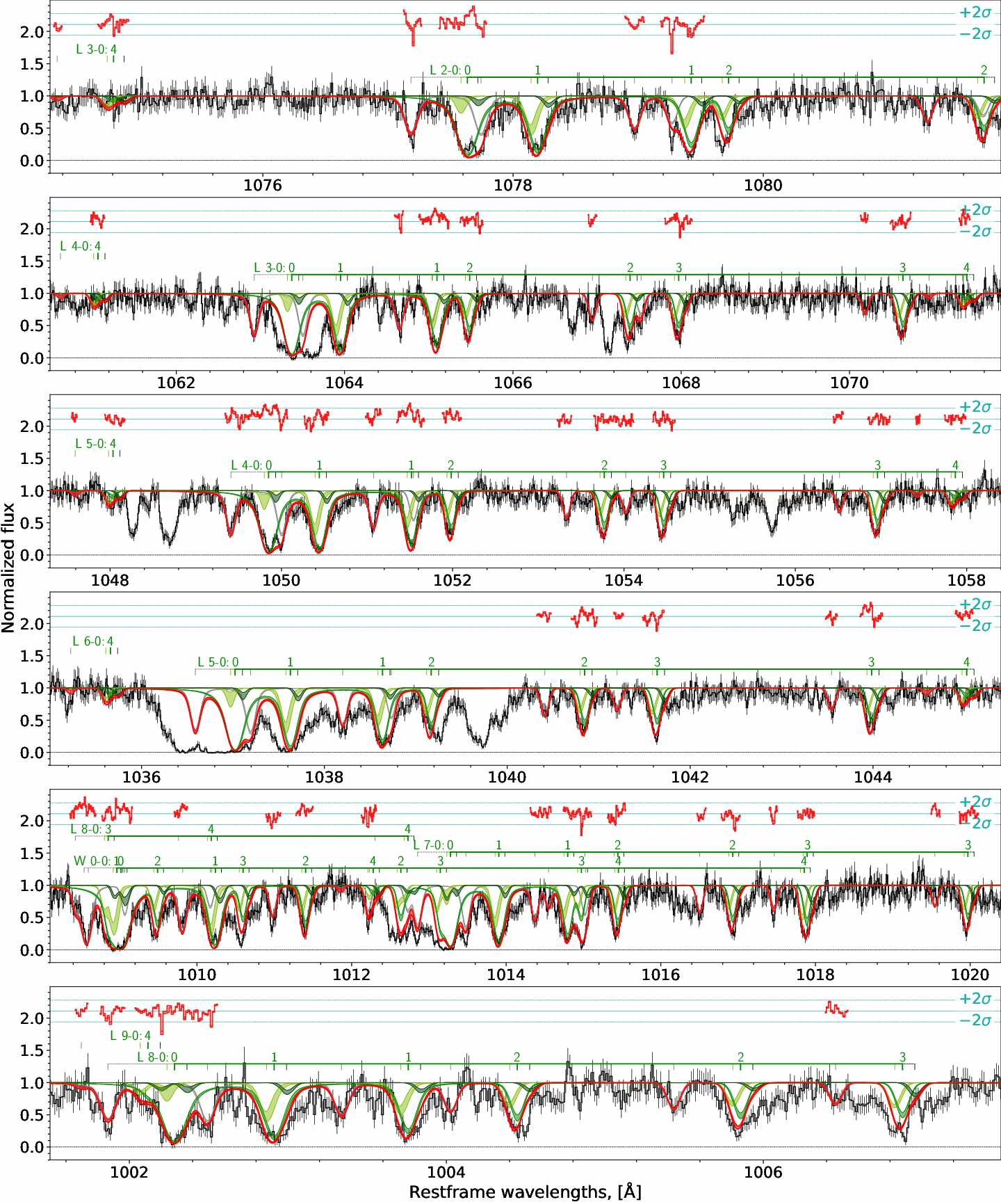
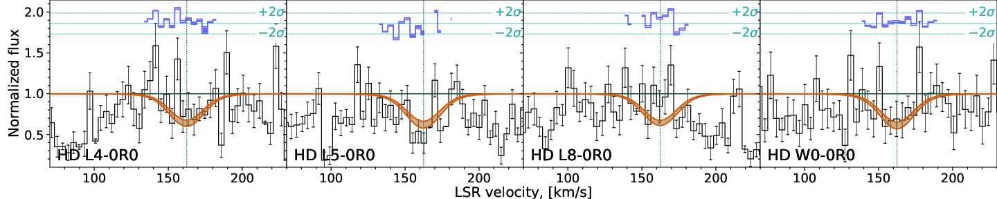
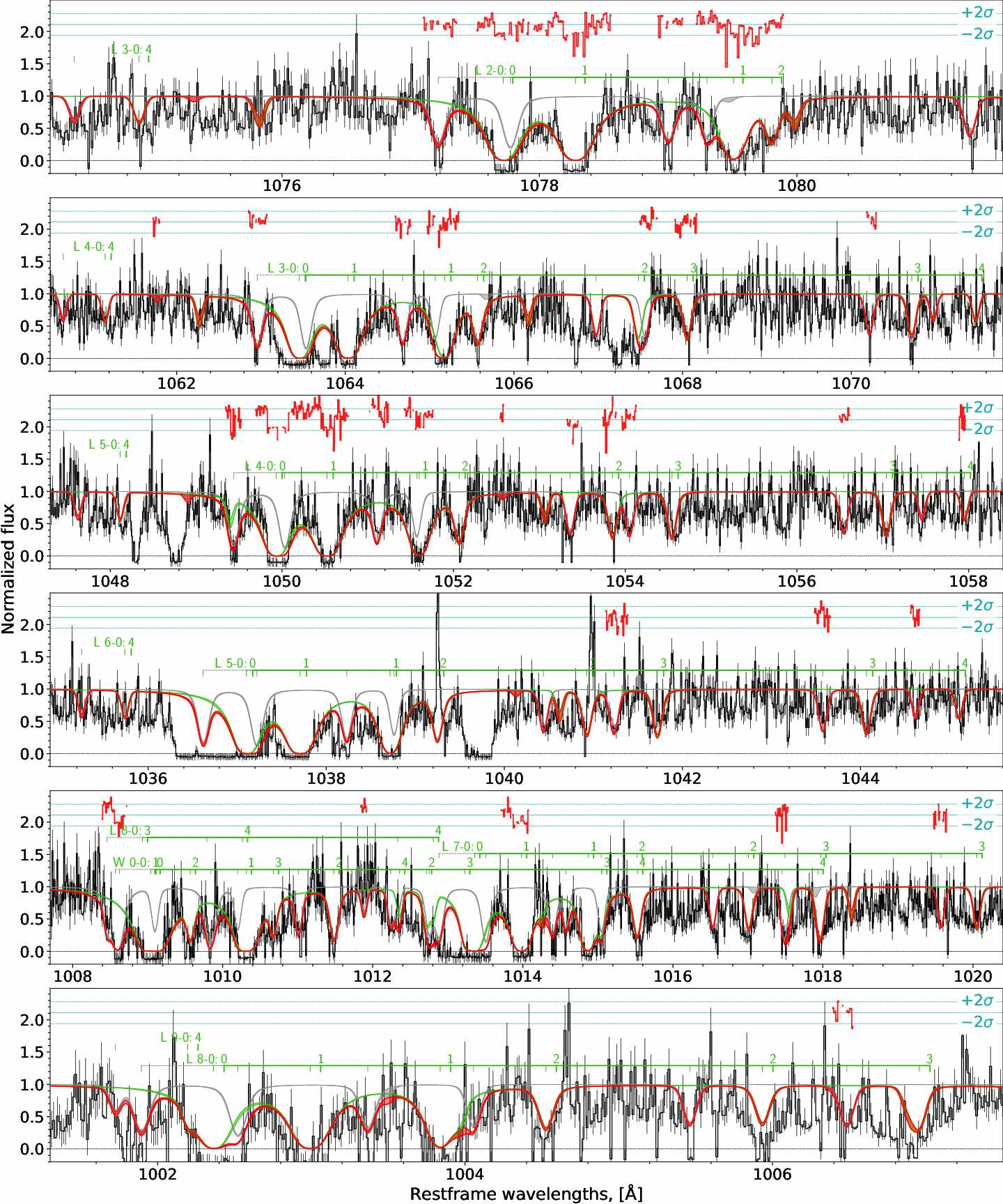
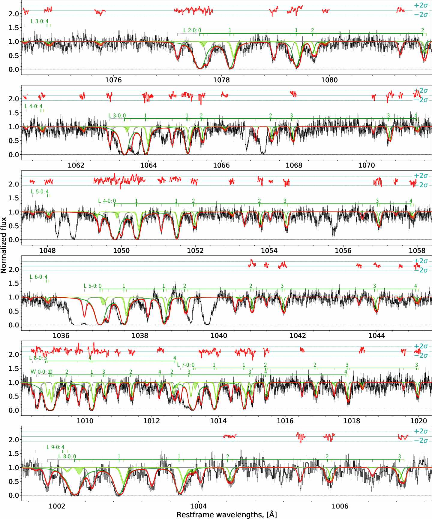
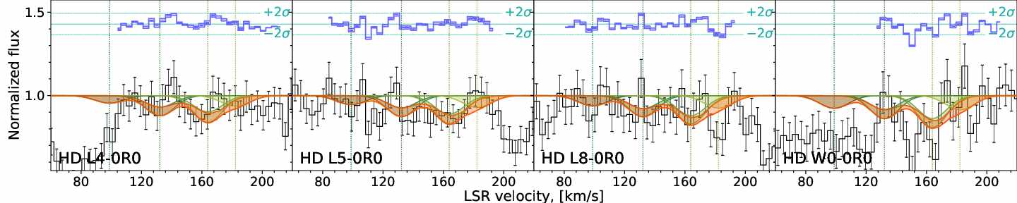
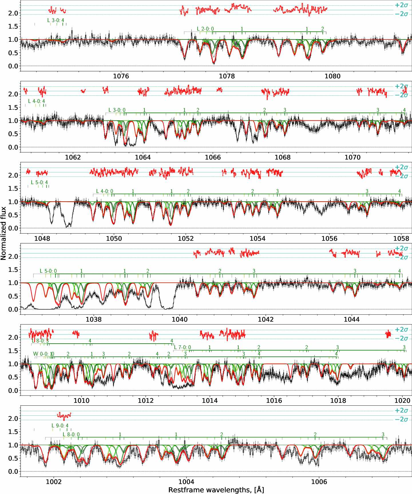
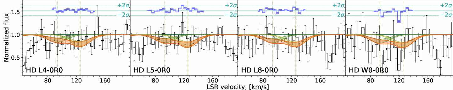
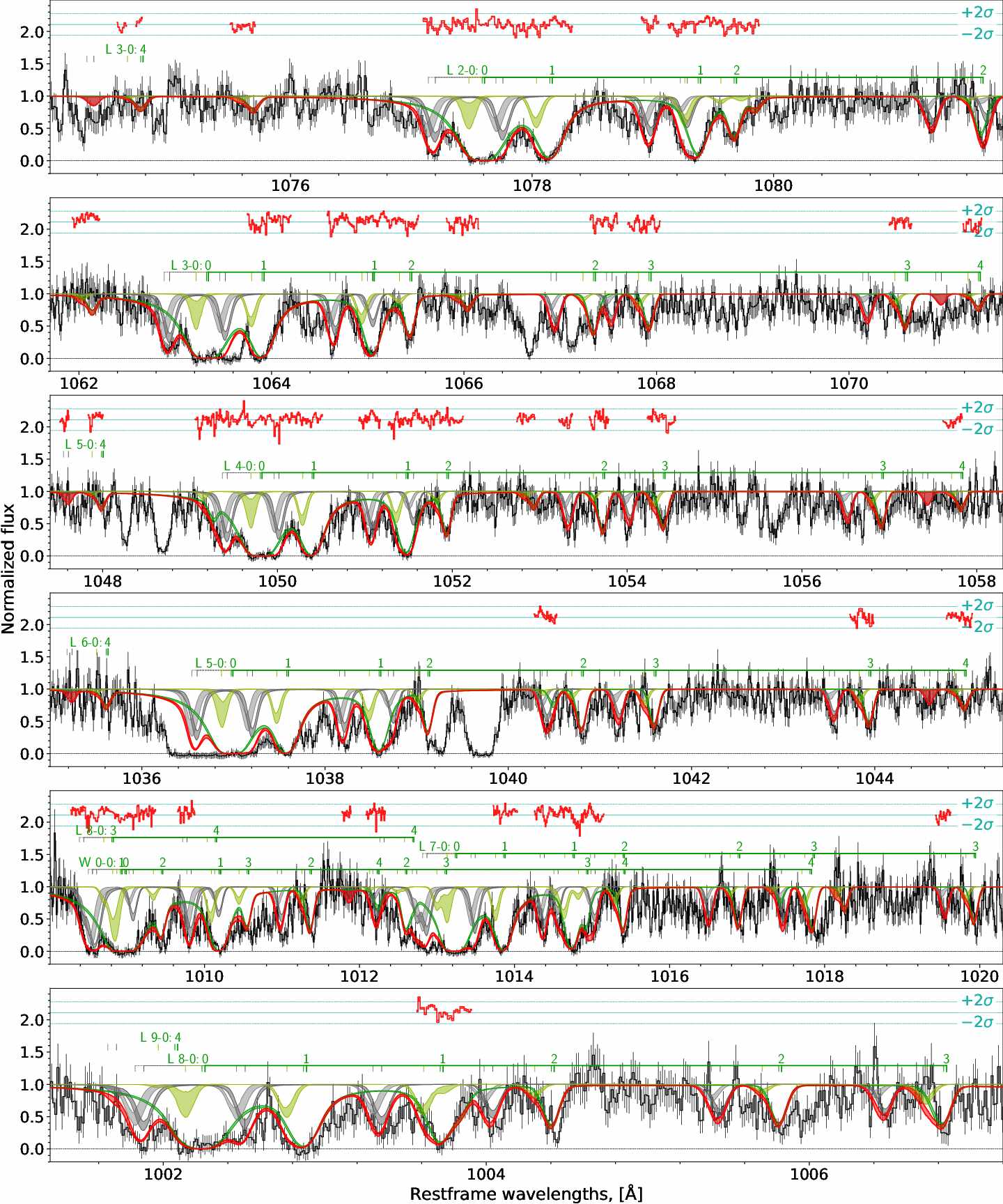
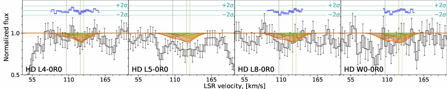
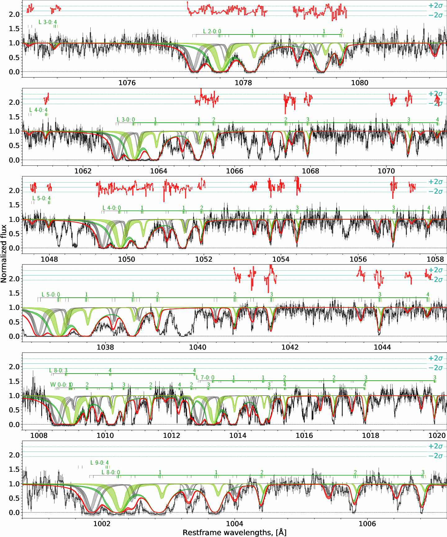
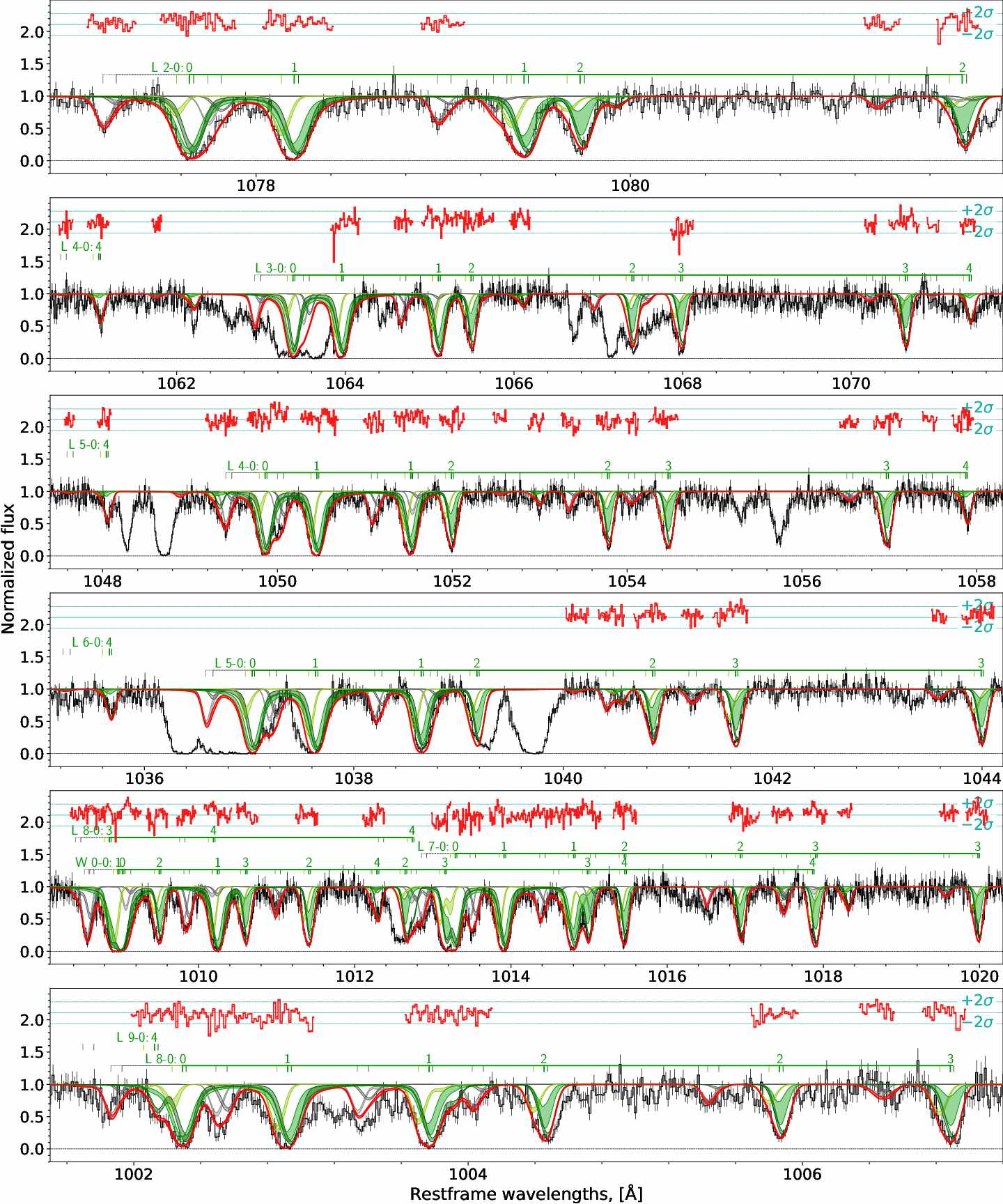
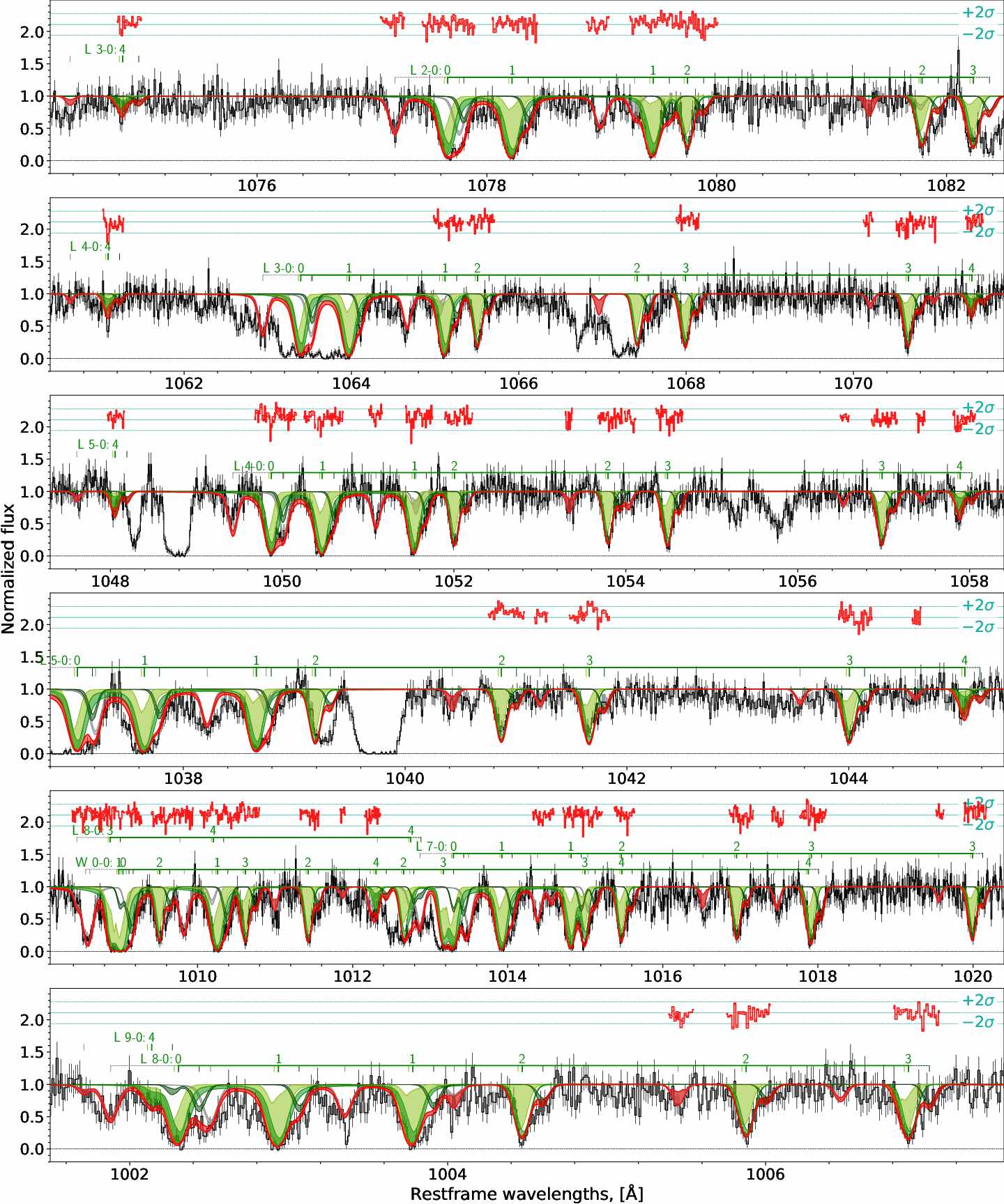
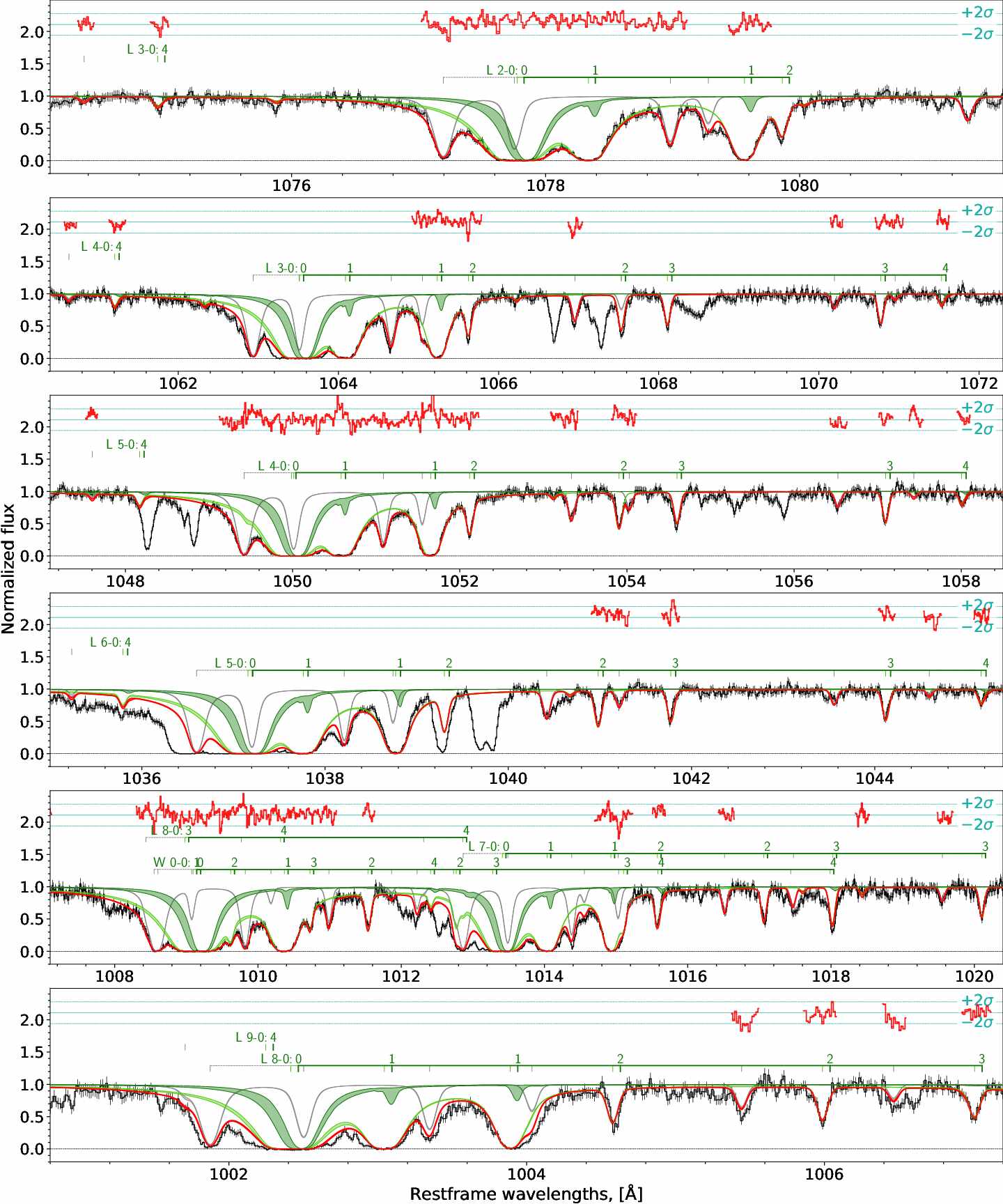
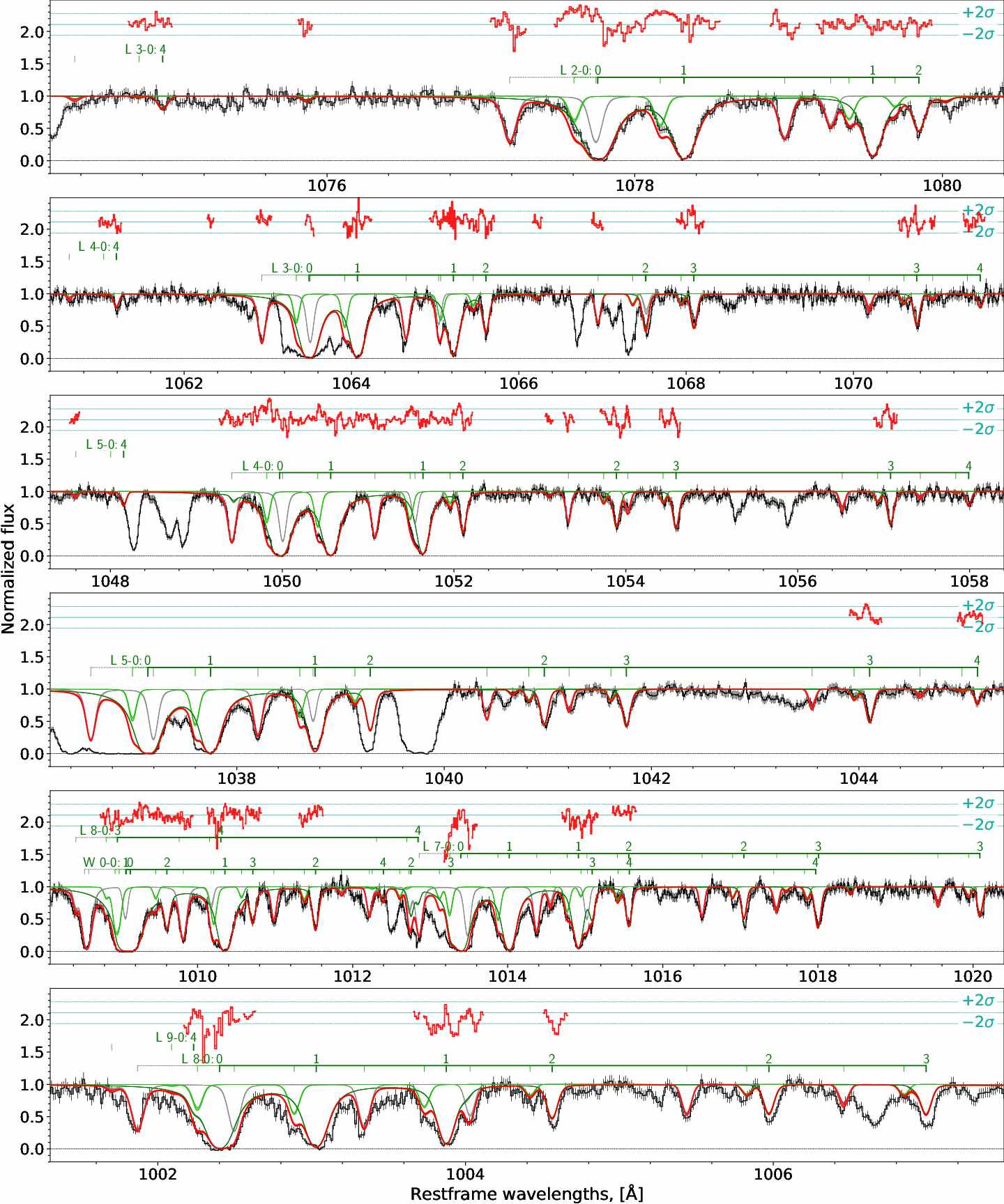
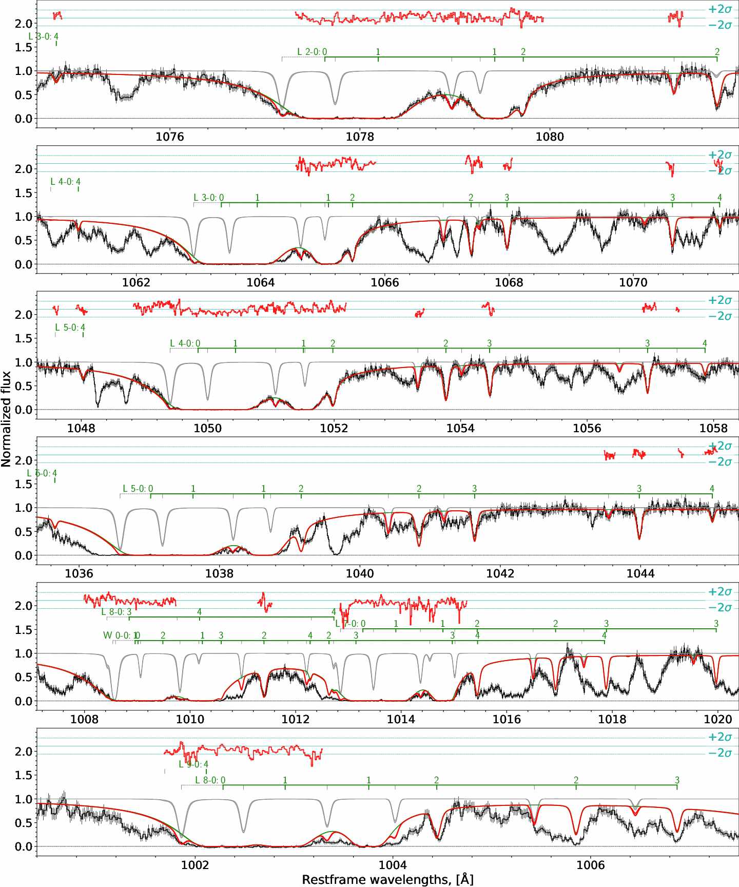
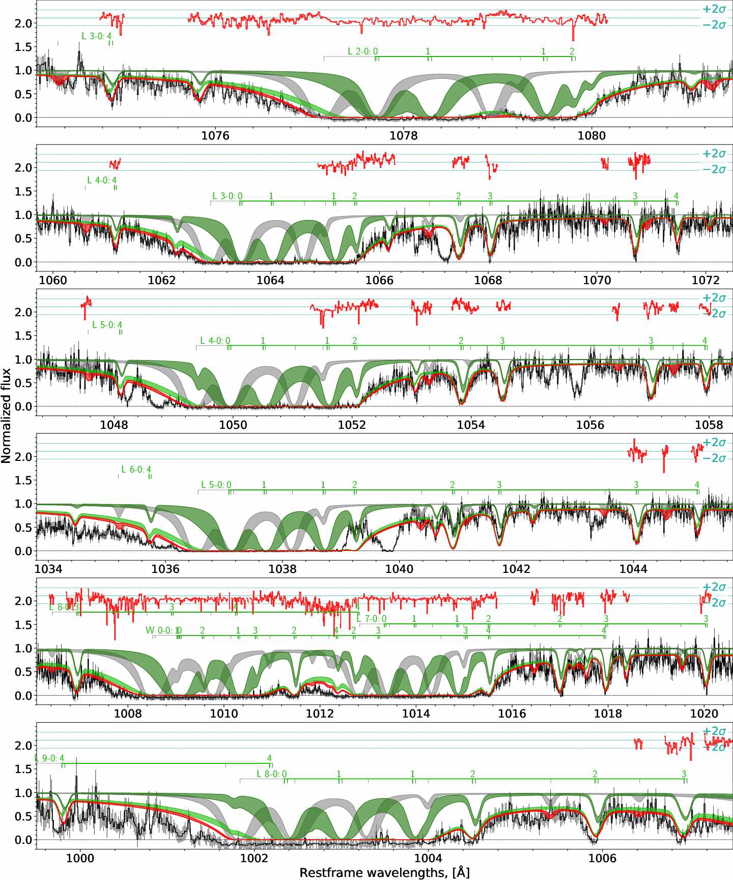
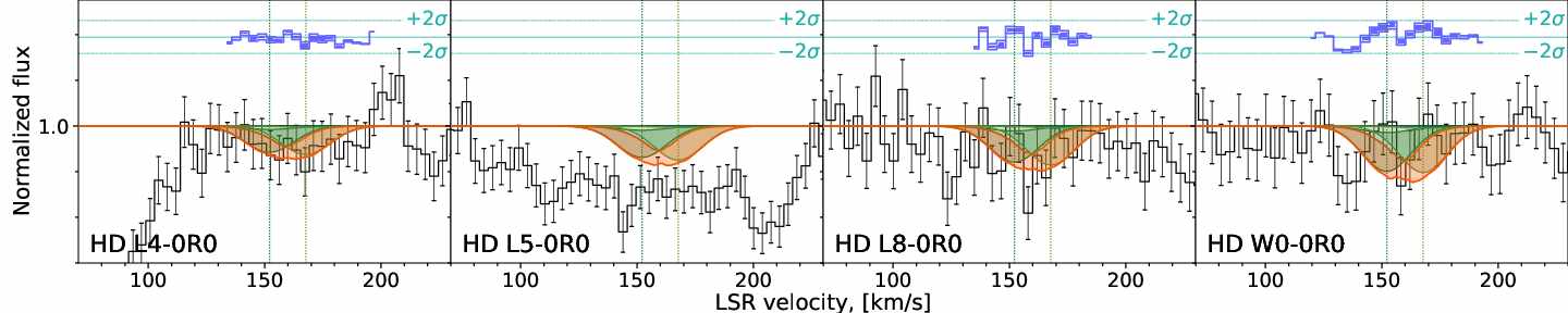
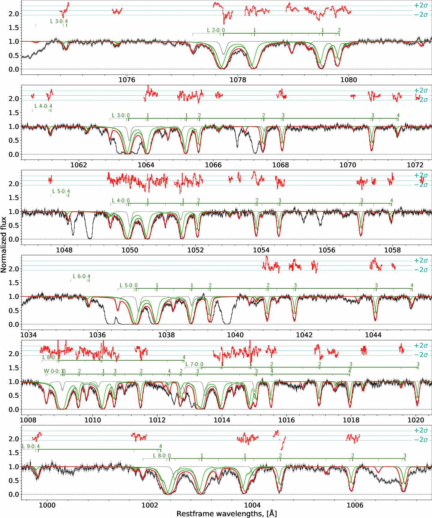
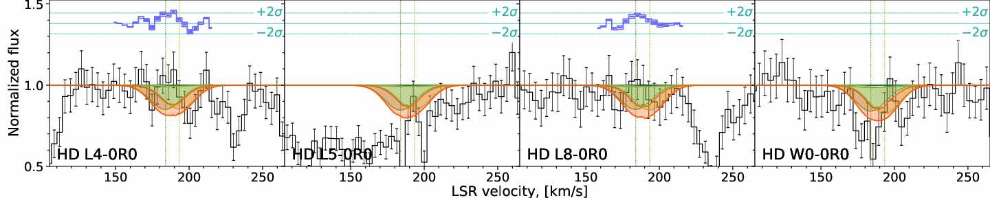
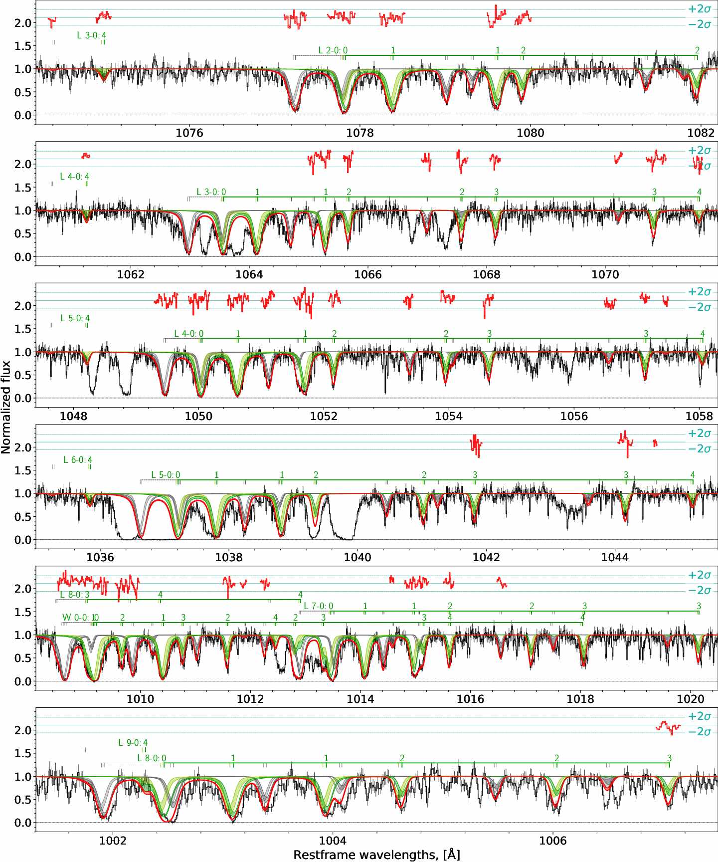
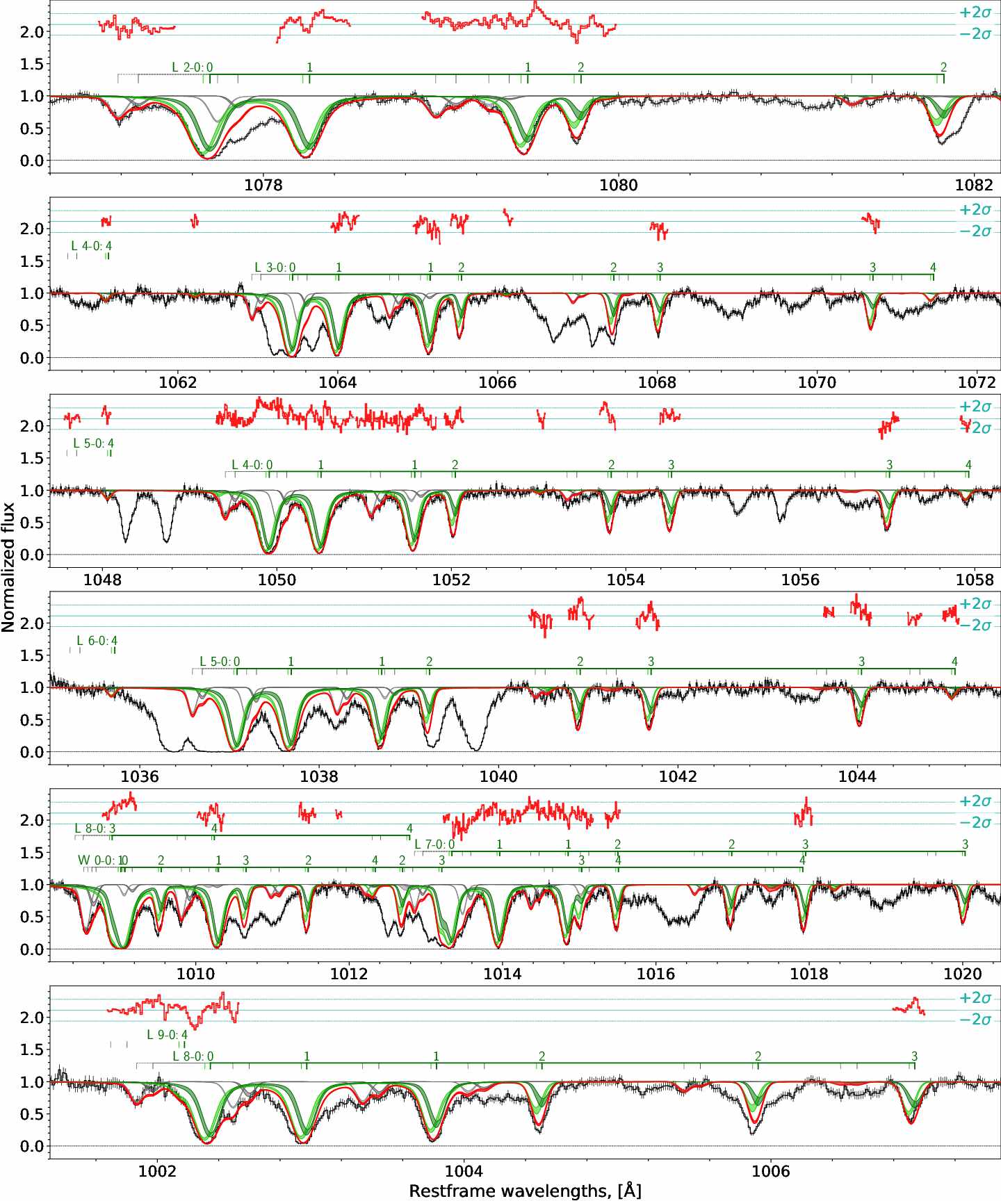
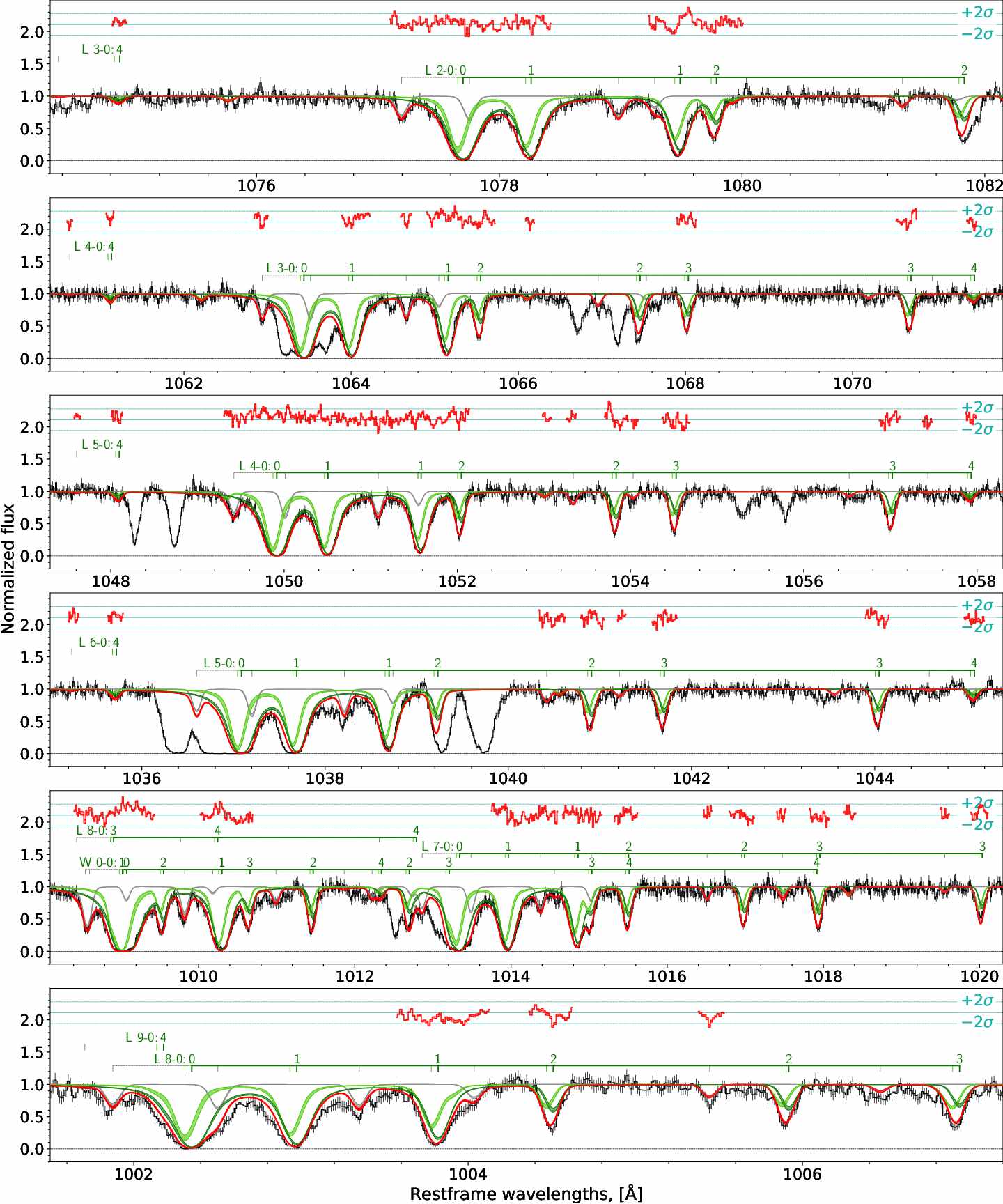
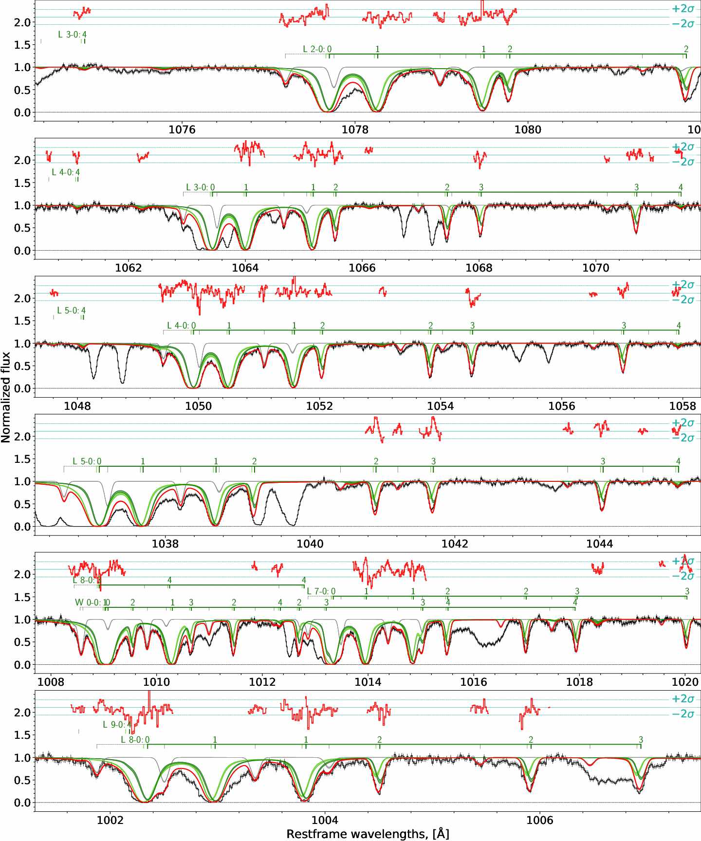
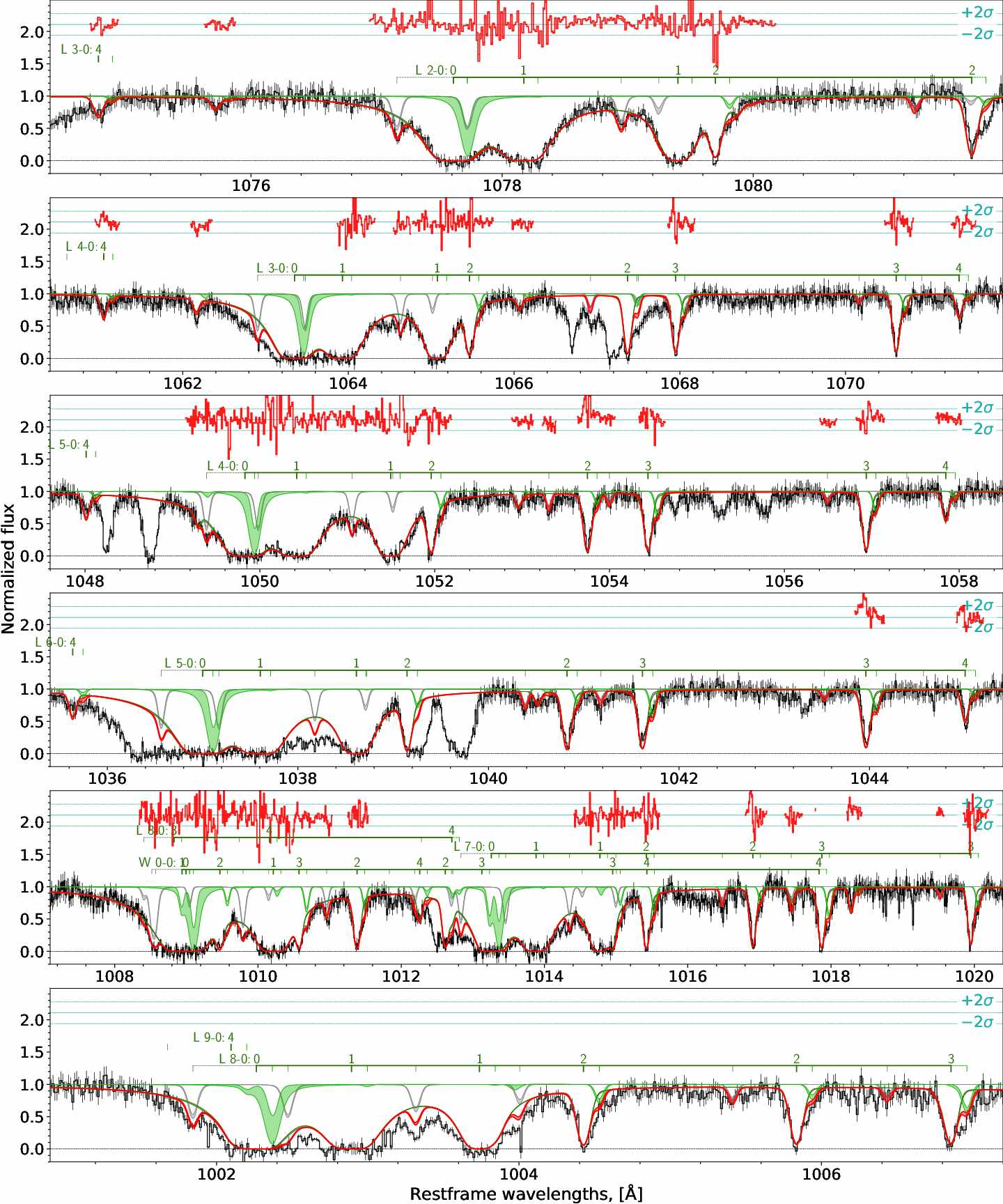
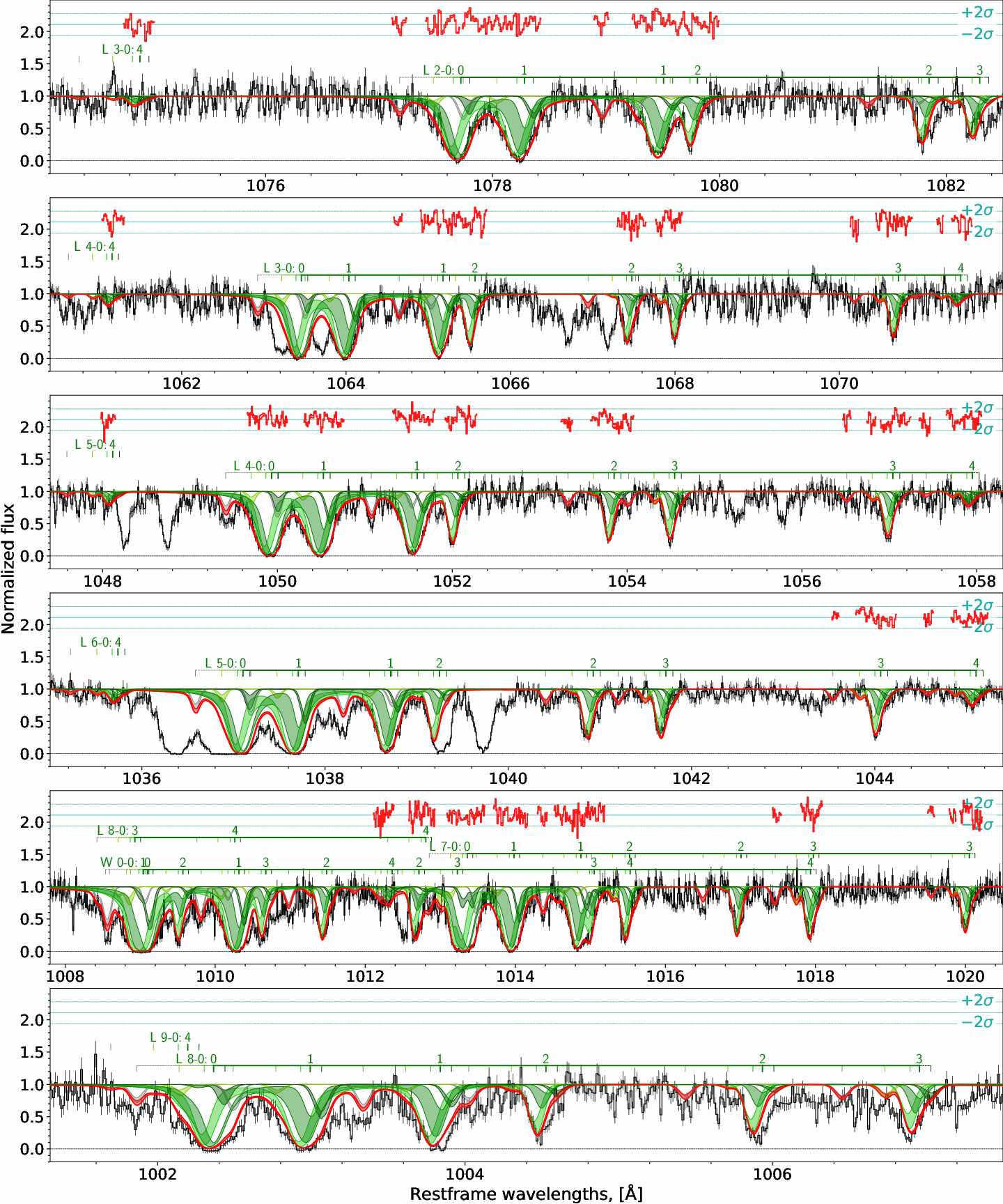
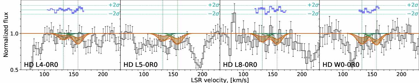
In the spectra of stars towards Magellanic Clouds there are typically two groups of the components: one from Milky Way disk and/or halo and another from LMC or SMC. In most of the cases each group can be resolved into few sub-components, that was fitted with profile fitting. In total, HD was detected towards 24 sightlines (among which in 19 there were new detections), and we placed upper limits on HD column densities in all others. The total H₂ and HD column densities derived from line profiles are shown in Tables 1 and 3 for LMC and SMC, respectively. Details on analysis of each systems are shown in Appendix B (see Supplementary materials). We show an example of line profile fitting of HD lines for the system towards Sk 191 in the SMC in the Figure 1; in the Appendix A we show all of the new HD detections. We also show an example of non-detection of HD lines in the Figure 119  in the system towards AV 14 in the SMC. In Figure 3 we show measured HD and H₂ column densities in the components and compared it with known measurement obtained in Milky Way and at high-redshifts. We note that since the resolution and spectral quality is not enough we predominantly obtained conservative limits on HD at the level $\log N({\rm HD})\lesssim 15-16$, which we also show in Figure 3.

We found a wide ($\approx 2$ dex) range of measured HD/H₂ ratios in Magellanic Clouds from the values below the Milky-Way measurements, to the values higher that the isotopic D/H ratio. However, at the intermediate H₂ column densities, HD abundance is very sensitive to the physical conditions (see Balashev & Kosenko, 2020), due to the sensitivity of the position of D/HD transition, and therefore is not a problem to explain such wide range. We additionally, note that there is an obvious selection effect in Fig. 3, that is we were limited with $\log N({\rm HD})\gtrsim 13.5$.

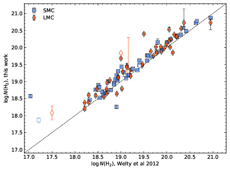
In Figure 4 we present comparison of the total H₂ column density obtained by Welty et al. 2012 with the our results, obtained using the sum over all components associated with LMC and SMC. One can see that $N({\rm H_{2}})$ values that we obtained are systematically higher ($\sim 0.3$ dex) then that obtained by Welty et al. 2012. It may arise, firstly, from differences in methods: for most of the systems Welty et al. 2012 fitted only J = 0 and 1 lines and for only about 40 systems in their sample they provided detailed fit assuming multiple components. This may lead to underestimation of their results. Secondly, the discrepancy may arise from difference and difficulties in the calibration of data and uncertainty in resolution of combined spectra after reduction. Thirdly, as was noted above, in our analysis we used MCMC method, which in some cases provide the results with relatively low Doppler parameters and therefore may overestimate column densities (in the Tables 1 and 3 such systems are denoted by item $e$) in the case of the low column densities $\log N\lesssim 19$, at which Lorentz wings are not yet evident. Such low ($b\gtrsim 1\rm\,km\,s^{-1}$) Doppler parameters are not surprising for cold clouds, and sometimes confirmed in high-resolution observations Carswell et al. 2011, e.g.. The Doppler parameters, under FUSE resolution (corresponding $b\approx 20\rm\,km\,s^{-1}$) mainly estimated from joint fit of lines with different oscillator strengths. However, since the FUSE spectrum has limited spectral range and number of available H₂ bands is typically limited to few. Therefore, high-resolution observations with larger wavelength range are needed to confirm a realm of such low Doppler parameter values. And the last, Welty et al. 2012 have not provided uncertainties on their column densities and we do not know real inconsistency between our results.

Figure 1: Fit to HD absorption lines towards Sk 191 in SMC. Here black line shows spectrum, while the coloured stripes show 0.683 credible interval of the line profiles sampled from posterior probability distributions of fitting parameters. The red represents the total line profile, while the green ones indicate individual components. In this particular spectrum, the green and red coincides, since there is only one component. Blue points at the top of each panel show residuals. Here we show only components found in Magellanic Clouds.

Figure 2: Fit to HD absorption lines towards AV 14 in SMC, which shows an example of non-detection of HD molecule. Lines are the same as for 1.

Figure 3: The HD versus H₂ column densities. The measurements in Small and Large Magellanic Clouds (this work) are shown by filled blue squares and red diamonds, respectively. Unfilled symbols represent the 3$\sigma$ upper limits on HD column densities. Green circles show the measurements towards quasars at high redshifts (see Kosenko et al., 2021, and references therein), yellow triangles indicate the measurements in our Galaxy (Snow et al., 2008) and solid the blue line and stripe show the primordial D/H ratio (Planck Collaboration et al., 2020).

Below we provide some details regarding several interesting sightlines.

4.1 Sk-67 5

The star is located in diffuse H ii region on the Western edge of LMC and the system have previously been studied by André et al. 2004, who used data, obtained by FUSE, HST/STIS and VLT/UVES.They found $\log N({\rm H_{2}})=19.44\pm 0.05$ which is in agreement with our value $\log N({\rm H_{2}})=19.47\pm 0.01$. Their value of HD column density is $13.62^{+0.09}_{-0.12}$, while we obtained a wider range $15.5^{+0.3}_{-2.1}$, which includes saturated solution for the fit (see Sect. 3). Indeed, to obtain HD column density André et al. 2004 used an average value between Apparent Optical Depth (AOD, Savage & Sembach 1991) method and line profile fitting, however it is known that AOD is not appropriate for lines with large optical depth and/or low resolution (above it was noted than resolution of FUSE spectra may be degraded after data reduction), therefore HD column density given by André et al. 2004 may be underestimated.

4.2 Sk-67 105

Sk-67 105 is one of the most massive eclipsing binary system (Niemela & Morrell, 1986) in the LMC, which probably reveals a contact configuration with 48.3$M_{\odot}$ and 31.4$M_{\odot}$ (Ostrov & Lapasset, 2003).

From H₂ lines (mostly from saturated $\rm J=0$ and 1) we found an evidence of partial coverage of absorption system towards Sk-67 105 which may arise from the configuration of the background radiation source. To get more reliable results we added a covering factor (see e.g. Balashev et al., 2011) as an independent parameter during the fit to H₂ lines, which value was found to be $0.888^{+0.002}_{-0.002}$. We could not detect HD in this system and placed upper limit on the column density in both H₂ components to be $\log N({\rm HD})\lesssim 14.8$ and $\lesssim 13.9$.

4.3 Sk-68 135

The star is located in the north of 30 Dor complex, one of the most studied star-forming regions and was previously studied by André et al. 2004.

Our HD column density estimate, $\log N({\rm HD})=14.0^{+0.6}_{-0.3}$ is consistent with the result obtained by André et al. 2004, $\log N({\rm HD})=14.15^{+0.11}_{-0.15}$, while we found H₂ column density to be a bit higher (our $\log N(\rm H_{2})=19.99\pm 0.01$ versus their $19.87\pm 0.05$; note that André et al. 2004 fitted H₂ assuming a single-component model, while we fitted H₂ with 2-components model). Roman-Duval et al. 2019 found H i column density in this system to be significantly lower then Welty et al. 2012. Roman-Duval et al. 2019 used Ly$\alpha$ from HST, while Welty et al. 2012 used Ly$\beta$ line from FUSE spectra, where the difficulties in H i column density estimation partly arises from large amount of H₂ absorption lines in the wings of Ly$\beta$. Additionally Welty et al. 2012 did not provide uncertainties of the $N(\rm HI)$ measurements. Analysis of Ly$\alpha$ provides more reliable result, therefore we took value from Roman-Duval et al. 2019.

4.4 Sk-69 246

This star belongs to 30 Dor complex and the system on the line-of-sight have previously been studied by Bluhm & de Boer 2001 and André et al. 2004.

Bluhm & de Boer 2001 used curve-of-growth method to estimate H₂ and HD column densities. Nevertheless, we got $\log N({\rm H_{2}})=19.76\pm 0.01$ and $\log N({\rm HD})=13.89\pm 0.06$ which is in agreement with results obtained by Bluhm & de Boer 2001. Comparing with André et al. 2004 we obtained that $\log N({\rm H_{2}})$ is close to their result ($19.66\pm 0.04$). They found HD to be lower then both values found by Bluhm & de Boer 2001 and us. André et al. 2004 used only L5, L8 and L14 HD lines, while we used L3, L5, L7 and W0 (we did not use neither L14, since spectra from 1A LiF channel do not cover this line, moreover this line is weak and noizy nor L8 since it is blended by H₂ and S ii absorptions). Also André et al. 2004 reported blend of L3 line, but we found that this line does not disagree with other HD lines so we included it in the analysis.

4.5 AV 95

The star AV 95 belongs to the bar of SMC and H₂ and HD in the system towards AV 95 have previously been studied by André et al. 2004.

Both our HD ($\log N({\rm HD})=13.75^{+0.39}_{-0.29}$) and H₂ ($\log N({\rm H_{2}})=19.48^{+0.03}_{-0.02}$) column densities are consistent with values $\log N({\rm H_{2}})=19.43\pm 0.04$ and $\log N({\rm HD})=13.82^{+0.96}_{-0.18}$) found by André et al. 2004, respectively.

4.6 AV 242

The star AV 242 is located to the south-west of the star-formation region NGC 346 in the SMC and it is a bow shock-producing star, moving towards NGC 346 (Gvaramadze et al., 2011). Among the absorption systems towards AV 242 we found an evidence of the high (or intermediate) velocity cloud (HVC) at $v=98.8$ km/s with $\log N({\rm H_{2}})=17.18^{+0.14}_{-0.16}$. To our knowledge, it is the first found HVC towards SMC, which contains H₂ molecules. Unfortunately, we could place only upper limits on the HD column density towards AV 242.

4.7 AV 488

The star AV 488 is located within Knot 1 region, in the wing of the SMC (a more quiescent region of SMC comparing with the bar).

Metals and H₂, HD and CO molecules have previously been studied by André et al. 2004. They have found H₂ and HD column densities to be $19.21\pm 0.06$ and $13.85^{+0.11}_{-0.14}$, respectively, which consist with our results within errors (total H₂ column density is $19.30^{+0.01}_{-0.02}$ and HD $13.6^{+0.6}_{-0.5}$).

Table 1: Fit results for HD and H₂ towards LMC.

Star	$\log N(\mbox{HI})^{a}$	$\Delta V^{b},\rm[km/s]$	$\log N(\mbox{H}_{2})$	$\log N(\mbox{HD})^{c}$
Sk-67 2	$21.00$	260.5	$20.46^{+0.15}_{-0.46}$	$\lesssim 17.1$
	’-’	280.3	$20.40^{+0.14}_{-0.20}$	$\lesssim 17.3$
Sk-67 5	$21.00$	294.7	$19.47^{+0.01}_{-0.01}$	$15.5^{+0.3}_{-2.1}$
Sk-66 1		286.3	$19.32^{+0.01}_{-0.01}$	$\lesssim 15.9$
Sk-67 20		283.2	$19.04^{+0.01}_{-0.01}$	$\lesssim 14.2$
Sk-66 18		274.5	$17.70^{+0.11}_{-0.12}$	$\lesssim 14.0$
		291.2	$18.17^{+0.05}_{-0.05}$	$\lesssim 15.7$
PGMW 3070		264.5	$18.14^{+0.04}_{-0.04}$	$\lesssim 15.6$
		286.5	$19.12^{+0.02}_{-0.01}$	$\lesssim 16.0$
LH 10-3073e,f		265.5	$19.27^{+0.01}_{-0.03}$	$14.3^{+0.9}_{-0.3}$
		285.8	$18.05^{+0.17}_{-0.14}$	$\lesssim 15.3$
LH 10-3102f		264.0	$17.51^{+0.11}_{-0.06}$	$14.2^{+0.4}_{-0.3}$
		285.0	$18.62^{+0.03}_{-0.01}$	$\lesssim 15.6$
		299.7	$14.65^{+0.07}_{-0.05}$	$\lesssim 15.7$
LH 10-3120	$21.48^{d}$	272.2	$18.22^{+0.03}_{-0.04}$	$\lesssim 15.3$
	’-’	289.1	$17.90^{+0.07}_{-0.05}$	$\lesssim 15.4$
PGMW 3157		266.9	$17.35^{+0.25}_{-0.38}$	$\lesssim 16.5$
		287.2	$19.13^{+0.03}_{-0.03}$	$\lesssim 16.5$
PGMW 3223	$21.4^{d}$	267.8	$18.78^{+0.02}_{-0.01}$	$\lesssim 15.9$
	’-’	287.8	$15.27^{+0.22}_{-0.17}$	$\lesssim 15.7$
Sk-66 35	$20.83^{d}$	264.4	$18.34^{+0.24}_{-0.18}$	$\lesssim 16.2$
	’-’	275.4	$19.35^{+0.07}_{-0.02}$	$\lesssim 15.9$
	’-’	286.0	$18.64^{+0.18}_{-0.13}$	$\lesssim 15.7$
Sk-69 52		248.8	$18.64^{+0.03}_{-0.02}$	$\lesssim 15.9$
Sk-65 21	$<20.50$	247.8	$18.38^{+0.01}_{-0.01}$	$\lesssim 15.9$
Sk-66 51e		311.5	$18.08^{+0.20}_{-0.20}$	$\lesssim 15.3$
Sk-70 79f	$21.26^{d}$	234.6	$20.38^{+0.01}_{-0.01}$	$15.6^{+0.7}_{-0.5}$
Sk-68 52	$21.30^{d}$	248.8	$19.51^{+0.01}_{-0.01}$	$\lesssim 15.6$
Sk-71 8	$21.04$	186.6	$18.21^{+0.04}_{-0.07}$	$\lesssim 16.4$
	’-’	220.4	$18.66^{+0.04}_{-0.03}$	$\lesssim 14.3$
Sk-70 85		256.7	$18.57^{+0.05}_{-0.04}$	$\lesssim 16.0$
		283.3	$17.18^{+0.18}_{-0.30}$	$\lesssim 15.9$
Sk-69 106		253.4	$18.78^{+0.02}_{-0.01}$	$\lesssim 15.6$
Sk-68 73f	$21.66^{d}$	294.2	$20.24^{+0.01}_{-0.01}$	$14.2^{+0.1}_{-0.1}$
Sk-67 105	$21.25^{d}$	301.9	$19.42^{+0.05}_{-0.01}$	$\lesssim 14.8$
	’-’	310.3	$17.46^{+0.29}_{-0.85}$	$\lesssim 13.9$
BI 184	$21.12^{d}$	240.4	$19.89^{+0.01}_{-0.02}$	$\lesssim 16.7$
	’-’	281.2	$16.78^{+0.11}_{-0.20}$	$\lesssim 15.8$
Sk-71 38		201.3	$17.46^{+0.07}_{-0.07}$	$\lesssim 16.1$
		243.0	$18.53^{+0.06}_{-0.04}$	$\lesssim 16.0$
		280.1	$17.45^{+0.06}_{-0.05}$	$\lesssim 14.7$
Sk-71 45	$21.09$	254.1	$18.55^{+0.01}_{-0.01}$	$\lesssim 13.3$
Sk-71 46f		243.4	$20.32^{+0.03}_{-0.04}$	$14.60^{+1.08}_{-0.30}$
Sk-69 191	$20.78^{d}$	229.2	$19.11^{+0.01}_{-0.02}$	$\lesssim 15.9$
	’-’	257.7	$15.34^{+0.92}_{-0.30}$	$\lesssim 15.1$

Table 2: continued

Star	$\log N(\mbox{HI})^{a}$	$\Delta V^{b},\rm[km/s]$	$\log N(\mbox{H}_{2})$	$\log N(\mbox{HD})^{c}$
J 0534-6932f	$21.60$	270.6	$19.88^{+0.01}_{-0.01}$	$14.5^{+0.9}_{-0.4}$
	’-’	294.3	$17.24^{+0.26}_{-0.41}$	$\lesssim 16.0$
BI 237f	$21.62$	296.2	$20.20^{+0.01}_{-0.01}$	$14.4^{+1.0}_{-0.2}$
Sk-68 129	$21.72$	276.0	$20.53^{+0.07}_{-0.03}$	$\lesssim 17.2$
Sk-69 220	$21.28$	283.3	$19.29^{+0.01}_{-0.01}$	$\lesssim 16.4$
Sk-69 223	$21.9$	273.0	$19.18^{+0.08}_{-0.10}$	$\lesssim 16.3$
	’-’	308.3	$19.94^{+0.01}_{-0.02}$	$\lesssim 16.2$
Sk-66 172	$21.25$	289.3	$18.18^{+0.08}_{-0.04}$	$\lesssim 16.1$
	’-’	301.5	$16.62^{+0.49}_{-0.19}$	$\lesssim 16.1$
	’-’	331.0	$16.35^{+0.30}_{-0.79}$	$\lesssim 14.9$
	’-’	375.3	$15.97^{+0.38}_{-0.67}$	$\lesssim 15.5$
Sk-69 228	$21.63$	262.2	$18.28^{+0.03}_{-0.13}$	$\lesssim 16.8$
	’-’	296.3	$18.87^{+0.06}_{-0.05}$	$\lesssim 16.4$
BI 253f	$21.67^{d}$	267.3	$20.01^{+0.01}_{-0.01}$	$15.3^{+0.4}_{-0.9}$
	’-’	279.9	$18.12^{+0.19}_{-0.35}$	$13.65^{+0.20}_{-0.23}$
Sk-68 135	$21.46^{d}$	250.7	$18.83^{+0.11}_{-0.06}$	$\lesssim 15.9$
	’-’	272.4	$19.99^{+0.01}_{-0.01}$	$14.0^{+0.6}_{-0.3}$
Sk-68 137f	$21.50$	278.5	$20.31^{+0.05}_{-0.32}$	$16.5^{+0.2}_{-1.6}$
	’-’	302.9	$20.53^{+0.05}_{-0.11}$	$14.5^{+1.1}_{-0.3}$
Brey 77	$21.79$	277.1	$19.30^{+0.04}_{-0.06}$	$\lesssim 15.7$
	’-’	296.1	$19.42^{+0.05}_{-0.04}$	$\lesssim 16.1$
	’-’	316.4	$18.10^{+0.11}_{-0.11}$	$\lesssim 16.4$
Sk-69 243e	$21.80$	271.0	$18.29^{+0.27}_{-0.19}$	$\lesssim 15.7$
	’-’	280.3	$19.34^{+0.07}_{-0.05}$	$\lesssim 15.6$
	’-’	290.0	$19.66^{+0.02}_{-0.04}$	$\lesssim 16.0$
	’-’	312.4	$16.80^{+0.45}_{-0.16}$	$\lesssim 16.1$
Sk-69 246	$21.47^{d}$	273.0	$19.76^{+0.01}_{-0.01}$	$13.89^{+0.06}_{-0.06}$
Sk-68 140	$21.47^{d}$	275.6	$20.40^{+0.03}_{-0.03}$	$\lesssim 17.1$
Sk-71 50	$21.18$	238.2	$19.47^{+0.03}_{-0.04}$	$\lesssim 16.7$
	’-’	267.5	$19.43^{+0.05}_{-0.05}$	$\lesssim 16.5$
	’-’	292.1	$19.15^{+0.05}_{-0.07}$	$\lesssim 16.8$
Sk-69 279	$21.59^{d}$	249.4	$19.19^{+0.23}_{-0.44}$	$\lesssim 17.1$
	’-’	265.9	$20.54^{+0.01}_{-0.03}$	$\lesssim 17.0$
Sk-68 155	$21.44^{d}$	289.5	$20.02^{+0.03}_{-0.05}$	$\lesssim 16.8$
	’-’	307.7	$19.03^{+0.40}_{-0.42}$	$\lesssim 16.4$
	’-’	333.7	$19.00^{+0.22}_{-0.63}$	$\lesssim 17.0$
Sk-69 297		249.6	$19.77^{+0.03}_{-0.03}$	$\lesssim 16.3$
		295.1	$19.07^{+0.05}_{-0.05}$	$\lesssim 16.4$
Sk-70 115	$21.13^{d}$	215.6	$19.97^{+0.01}_{-0.01}$	$\lesssim 16.3$
	’-’	292.1	$18.23^{+0.03}_{-0.02}$	$\lesssim 15.5$

• $a$ Total H i column density, taken from Welty et al. 2012, the typical uncertainty is about $10\%$ (but the values were not shown by Welty et al. 2012) except systems denoted by $d$

• $b$ Kinematic shift of the component relative to the local standard of rest.

• $c$ Upper limits were constrained from $3\sigma$ confidence interval.

• $d$ Taken from Roman-Duval et al. 2019.

• $e$ Low Doppler parameter, hence $\log N(\rm H_{2})$ may be overestimated.

• $f$ Systems with new HD detections.

Table 3: Fit results for HD and H₂ towards SMC.

Star	$\log N(\mbox{HI})^{a}$	$\Delta V^{b},\rm[km/s]$	$\log N(\mbox{H}_{2})$	$\log N(\mbox{HD})^{c}$
AV 6	$21.54$	107.4	$16.82^{+0.26}_{-0.46}$	$\lesssim 15.9$
	’-’	132.0	$19.09^{+0.03}_{-0.02}$	$\lesssim 16.0$
	’-’	150.5	$17.42^{+0.15}_{-0.67}$	$\lesssim 16.2$
AV 14	$21.76$	91.5	$15.69^{+0.44}_{-0.29}$	$\lesssim 14.4$
	’-’	111.6	$18.18^{+0.07}_{-0.05}$	$\lesssim 14.1$
	’-’	131.2	$18.33^{+0.07}_{-0.07}$	$\lesssim 15.3$
	’-’	148.7	$16.60^{+0.25}_{-0.87}$	$\lesssim 15.4$
AV 15	$21.58$	119.9	$16.69^{+0.13}_{-0.12}$	$\lesssim 15.0$
		137.7	$18.45^{+0.01}_{-0.03}$	$\lesssim 15.3$
AV 16		128.0	$20.06^{+0.10}_{-0.07}$	$\lesssim 16.7$
		152.1	$19.99^{+0.10}_{-0.11}$	$\lesssim 16.4$
AV 18f	$22.04$	103.4	$16.04^{+0.22}_{-0.15}$	$\lesssim 15.6$
	’-’	130.6	$20.46^{+0.03}_{-0.02}$	$14.63^{+0.28}_{-0.20}$
	’-’	154.2	$19.19^{+0.17}_{-0.26}$	$14.6^{+1.0}_{-0.2}$
	’-’	176.0	$19.83^{+0.05}_{-0.06}$	$\lesssim 16.2$
AV 22	$<20.80$	112.4	$18.06^{+0.06}_{-0.08}$	$\lesssim 16.0$
	’-’	133.4	$17.50^{+0.18}_{-0.03}$	$\lesssim 15.8$
	’-’	153.8	$17.48^{+0.14}_{-0.08}$	$\lesssim 16.2$
AV 26f	$21.70$	119.3	$19.19^{+0.24}_{-0.22}$	$\lesssim 16.7$
	’-’	132.5	$20.70^{+0.02}_{-0.01}$	$14.4^{+1.7}_{-0.4}$
	’-’	152.0	$18.66^{+0.40}_{-0.77}$	$\lesssim 16.4$
AV 39a	$21.74$	103.7	$17.22^{+0.21}_{-0.26}$	$\lesssim 16.1$
	’-’	117.1	$18.66^{+0.04}_{-0.04}$	$\lesssim 15.5$
	’-’	129.8	$17.08^{+0.44}_{-0.22}$	$\lesssim 16.3$
AV 47	$21.32$	116.5	$17.72^{+0.07}_{-0.02}$	$\lesssim 15.4$
	’-’	129.1	$18.45^{+0.02}_{-0.02}$	$\lesssim 13.5$
AV 60a	$21.81$	125.0	$18.76^{+0.13}_{-0.13}$	$\lesssim 15.9$
	’-’	143.6	$19.72^{+0.02}_{-0.03}$	$\lesssim 16.6$
	’-’	217.7	$18.12^{+0.15}_{-0.05}$	$\lesssim 16.1$
AV 69	$21.59$	112.8	$18.34^{+0.05}_{-0.05}$	$\lesssim 15.1$
	’-’	128.4	$18.89^{+0.02}_{-0.02}$	$\lesssim 15.3$
AV 75	$21.79$	113.4	$18.87^{+0.01}_{-0.02}$	$\lesssim 15.3$
	’-’	126.7	$17.74^{+0.11}_{-0.08}$	$\lesssim 13.7$
AV 80f	$21.81$	118.8	$20.24^{+0.01}_{-0.01}$	$14.50^{+0.03}_{-0.04}$
	’-’	135.0	$18.75^{+0.24}_{-0.86}$	$\lesssim 15.4$
AV 81		111.9	$15.99^{+0.18}_{-0.10}$	$\lesssim 15.1$
		139.8	$18.58^{+0.03}_{-0.02}$	$\lesssim 15.5$
		177.3	$17.88^{+0.04}_{-0.08}$	$\lesssim 13.8$
AV 95	$21.49$	93.7	$15.46^{+0.05}_{-0.06}$	$\lesssim 13.4$
	’-’	124.5	$19.23^{+0.03}_{-0.04}$	$13.75^{+0.39}_{-0.29}$
	’-’	139.0	$19.11^{+0.05}_{-0.05}$	$\lesssim 13.6$
AV 104	$21.45$	119.4	$19.35^{+0.01}_{-0.01}$	$\lesssim 16.1$
	’-’	147.5	$16.77^{+0.28}_{-0.44}$	$\lesssim 15.9$

Table 4: continued

Star	$\log N(\mbox{HI})^{a}$	$\Delta V^{b},\rm[km/s]$	$\log N(\mbox{H}_{2})$	$\log N(\mbox{HD})^{c}$
AV 170	$21.14$	138.1	$19.73^{+0.01}_{-0.01}$	$\lesssim 16.1$
AV 175		121.7	$19.49^{+0.17}_{-0.12}$	$\lesssim 16.6$
		138.5	$20.05^{+0.10}_{-0.09}$	$\lesssim 16.4$
NGC 346-12	$21.81$	138.9	$19.64^{+0.17}_{-0.07}$	$\lesssim 13.4$
	’-’	166.5	$18.87^{+0.46}_{-0.51}$	$\lesssim 15.6$
	’-’	183.3	$20.40^{+0.04}_{-0.06}$	$\lesssim 13.6$
AV 207	$21.43$	160.1	$19.52^{+0.02}_{-0.04}$	$\lesssim 16.8$
	’-’	181.2	$18.93^{+0.08}_{-0.12}$	$\lesssim 16.5$
AV 208f	$21.85$	160.1	$19.82^{+0.09}_{-0.12}$	$14.5^{+1.0}_{-0.3}$
	’-’	181.2	$19.88^{+0.07}_{-0.16}$	$\lesssim 16.8$
AV 210	$21.85$	129.3	$19.33^{+0.01}_{-0.02}$	$\lesssim 16.1$
	’-’	164.8	$17.62^{+0.26}_{-0.34}$	$\lesssim 16.6$
	’-’	182.1	$17.34^{+0.16}_{-0.22}$	$\lesssim 16.5$
AV 215	$21.86$	126.2	$19.38^{+0.05}_{-0.10}$	$\lesssim 16.6$
	’-’	145.7	$19.52^{+0.06}_{-0.05}$	$\lesssim 16.5$
AV 216	$21.64$	124.7	$17.68^{+0.16}_{-0.22}$	$\lesssim 15.7$
	’-’	139.1	$18.71^{+0.05}_{-0.02}$	$\lesssim 16.0$
	’-’	162.5	$15.99^{+0.31}_{-0.22}$	$\lesssim 16.2$
NGC 346-637	$21.65$	162.4	$19.44^{+0.02}_{-0.02}$	$\lesssim 17.0$
AV 243	$21.52$	128.4	$18.95^{+0.02}_{-0.02}$	$\lesssim 15.7$
	’-’	147.9	$17.25^{+0.18}_{-0.30}$	$\lesssim 16.1$
AV 242e	$21.32$	98.8	$17.18^{+0.14}_{-0.16}$	$\lesssim 14.0$
	’-’	132.2	$15.00^{+0.16}_{-0.04}$	$\lesssim 15.7$
	’-’	163.9	$17.73^{+0.08}_{-0.11}$	$\lesssim 15.9$
	’-’	182.2	$16.75^{+0.14}_{-0.17}$	$\lesssim 14.9$
AV 261	$21.43$	93.2	$16.54^{+1.12}_{-0.37}$	$\lesssim 16.5$
	’-’	125.3	$19.38^{+0.03}_{-0.03}$	$\lesssim 16.7$
AV 266		106.4	$17.01^{+0.27}_{-0.68}$	$\lesssim 15.2$
		127.3	$19.81^{+0.01}_{-0.02}$	$\lesssim 15.6$
		132.5	$17.46^{+0.44}_{-0.23}$	$\lesssim 15.5$
AV 304	$21.48$	121.0	$19.55^{+0.03}_{-0.03}$	$\lesssim 15.8$
	’-’	137.6	$18.77^{+0.19}_{-0.27}$	$\lesssim 15.7$
AV 372f	$21.57$	122.6	$15.52^{+0.15}_{-0.05}$	$\lesssim 15.6$
	’-’	140.9	$18.62^{+0.04}_{-0.21}$	$\lesssim 16.2$
	’-’	147.1	$18.45^{+0.10}_{-0.18}$	$13.97^{+0.22}_{-0.23}$
AV 374	$21.14$	86.5	$18.09^{+0.03}_{-0.04}$	$\lesssim 16.2$
	’-’	133.1	$18.65^{+0.02}_{-0.02}$	$\lesssim 15.9$
AV 423	$21.49$	141.8	$18.00^{+0.36}_{-0.34}$	$\lesssim 15.5$
	’-’	145.6	$18.49^{+0.10}_{-0.11}$	$\lesssim 14.2$
	’-’	184.1	$17.03^{+0.28}_{-0.20}$	$\lesssim 16.1$
AV 435f	$21.54$	177.4	$19.92^{+0.01}_{-0.01}$	$15.6^{+0.2}_{-0.8}$
AV 440	$21.38$	130.5	$17.29^{+0.04}_{-0.03}$	$\lesssim 14.8$
	’-’	173.5	$19.06^{+0.01}_{-0.01}$	$\lesssim 15.8$
AV 472f		137.8	$20.38^{+0.01}_{-0.01}$	$15.9^{+0.3}_{-0.8}$
AV 476	$21.85$	157.4	$20.84^{+0.03}_{-0.05}$	$\lesssim 17.1$
	’-’	167.1	$19.79^{+0.21}_{-0.35}$	$\lesssim 17.1$

Table 5: continued

Star	$\log N(\mbox{HI})^{a}$	$\Delta V^{b},\rm[km/s]$	$\log N(\mbox{H}_{2})$	$\log N(\mbox{HD})^{c}$
AV 479	$21.42$	152.1	$18.73^{+0.01}_{-0.02}$	$\lesssim 15.2$
	’-’	167.8	$18.99^{+0.01}_{-0.01}$	$\lesssim 15.4$
AV 480	$21.42$	183.8	$18.21^{+0.10}_{-0.16}$	$\lesssim 16.1$
	’-’	193.4	$18.53^{+0.07}_{-0.07}$	$\lesssim 16.2$
AV 483	$21.13$	145.9	$18.71^{+0.03}_{-0.04}$	$\lesssim 16.1$
	’-’	157.2	$18.48^{+0.06}_{-0.04}$	$\lesssim 16.4$
AV 486f	$21.18$	145.5	$18.56^{+0.07}_{-0.07}$	$\lesssim 15.6$
	’-’	157.6	$19.07^{+0.02}_{-0.03}$	$14.0^{+0.9}_{-0.4}$
AV 488	$21.15$	146.6	$19.04^{+0.01}_{+0.03}$	$13.6^{+0.6}_{-0.5}$
	’-’	158.5	$18.96^{+0.03}_{-0.02}$	$\lesssim 14.6$
AV 490f	$21.46$	132.0	$19.88^{+0.01}_{-0.01}$	$16.1^{+0.2}_{-0.7}$
	’-’	162.7	$17.94^{+0.29}_{-0.39}$	$\lesssim 15.6$
AV 491	$21.40$	97.7	$15.66^{+0.47}_{-0.71}$	$\lesssim 14.7$
	’-’	143.6	$18.99^{+0.05}_{-0.10}$	$\lesssim 15.5$
	’-’	155.6	$18.98^{+0.05}_{-0.26}$	$\lesssim 15.0$
	’-’	184.4	$15.09^{+0.81}_{-0.06}$	$\lesssim 14.6$
AV 506	$21.35$	132.3	$16.36^{+0.29}_{-0.12}$	$\lesssim 14.0$
	’-’	147.5	$19.03^{+0.01}_{-0.01}$	$\lesssim 15.7$
Sk 191f	$21.51$	153.5	$20.78^{+0.02}_{-0.03}$	$14.7^{+1.2}_{-0.2}$
WR 9e	$21.48$	87.7	$16.06^{+0.34}_{-0.25}$	$\lesssim 15.7$
	’-’	117.8	$18.69^{+0.08}_{-0.05}$	$\lesssim 15.9$
	’-’	135.5	$19.37^{+0.01}_{-0.02}$	$\lesssim 15.7$
	’-’	149.9	$16.43^{+0.42}_{-0.19}$	$\lesssim 15.7$
	’-’	167.9	$17.37^{+0.11}_{-0.44}$	$\lesssim 15.9$

• $a$ Total H i column density, taken from Welty et al. 2012

• $b$ Kinematic shift of the component relative to the local standard of rest.

• $c$ Upper limits were constrained from $3\sigma$ confidence interval

• $e$ low Doppler parameter, $\log N(\rm H_{2})$ may be overestimated

• $f$ Systems with new HD detections.

Figure 4: Comparison between the total H₂ column density estimates obtained by Welty et al. 2012 (x-axis) and our results (y-axis). The blue squares and red diamonds show measurements in SMC and LMC, respectively. Open symbols show systems with low Doppler parameters (for details see text). Dashed black line shows the one-to-one ratio.

5 Cosmic-ray ionization rate

We used column densities, reported in the previous sections, to constrain physical conditions in the medium of LMC and SMC, associated with absorption systems. Among the parameters, listed above, in this work we focus mainly on CRIR (estimation of $n$, $\chi$ and metallicity in Magellanic Clouds will be presented in the accompanied paper, Kosenko et al in prep.) We followed the procedure developed and used for high-redshift systems in Kosenko et al. 2021.

This method is based on the balance equation between formation and destruction of HD molecules in the plane-parallel steady-state cloud, therefore leading to solve only one differential equation (Balashev & Kosenko, 2020):

$$\dfrac{{\rm d}N({\rm HD})}{{\rm d}N({\rm H_{2}})}=f(\zeta,n,\chi,Z,N({\rm H_{2}})),$$

except modelling of the cloud using full chemical network. Certainly to get reasonable constrain on CRIR this method requires an estimates of number density, UV field intensity and metallicity to remove degeneracy of parameters, which will be presented in Kosenko et al in prep. We fixed metallicity and used constraints on $n$ and $\chi$ as priors during the Bayesian inference. For $\zeta$ we used flat priors in log space, emulating a wide distribution. We used Markov Chain Monte-Carlo method to estimate posterior distribution function on CRIR. Results are shown in the last column of Table 6.

Unfortunately, in the most sightlines except one, we get only upper limits on CRIR, $\zeta$, due to large uncertainties in HD column density estimates (which is connected with insufficient quality of the data). In the systems, denoted by $\dagger$ in the Table 6, we could not constrain CRIR at all within the physically reasonable range $\lesssim 10^{-13}$, where the model from (Balashev & Kosenko, 2020) is appropriate. For these systems we got too wide posterior probabilities in this region (also due to the large uncertainties in $N({\rm HD})$) encompassing all the range for $\zeta$.

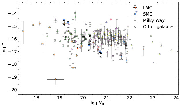
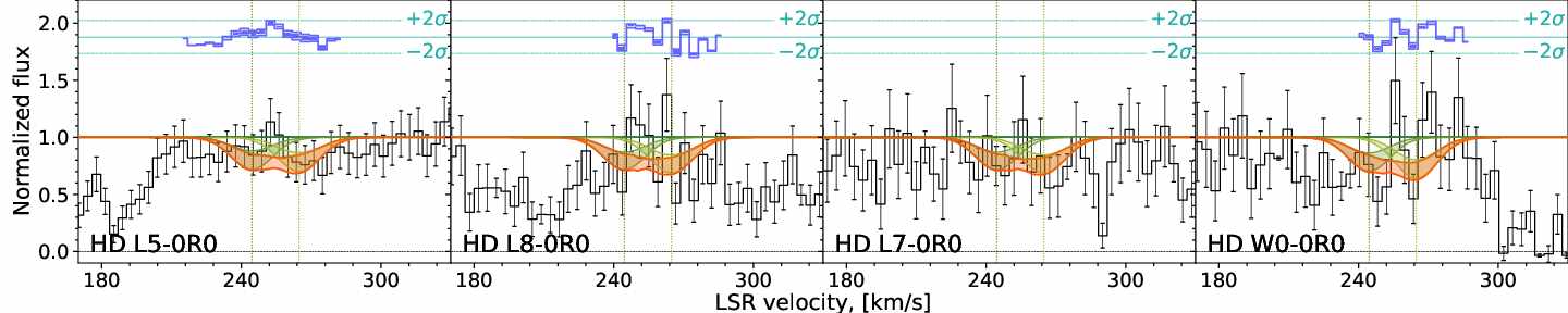
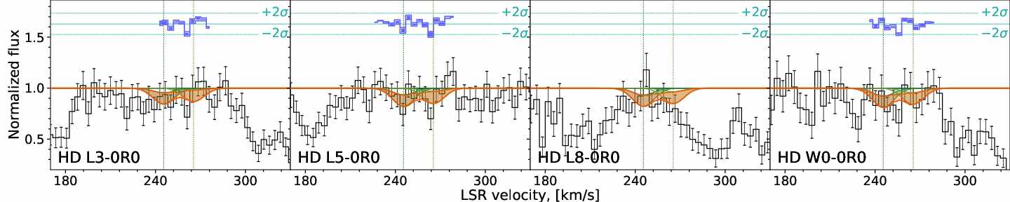
Constraints on CRIR as a function of H₂ column density are shown in the Fig. 5 (red diamonds for the LMC and blue squares for the SMC) and compared to other known CRIR estimations in the Milky Way and other galaxies. Note that constraint on $\zeta$ in the system towards Sk 191 in the LMC should be taken with caution since we got metallicity about an order lower than average value in SMC and it may be attributed to the large depletion in this system (one of the highest value of H₂ column density also may point at this; details will be provided in Kosenko et al. in prep.).

Table 6: Physical conditions derived in the absorption systems associated with LMC and SMC.

Star	$\rm[X/H]$	$\rm X$	$\log n[\rm cm^{-3}]$	$\log\chi$	$\log\zeta[\rm s^{-1}]$
LMC
Sk-67 5†	$-0.58^{+0.05}_{-0.05}$	Zn	$1.99^{+0.17}_{-0.18}$	$0.40^{+0.19}_{-0.18}$	–
Sk-70 79†	$-0.63^{+0.06}_{-0.05}$	Zn	$2.75^{+0.36}_{-0.31}$	$1.81^{+0.21}_{-0.18}$	–
Sk-71 46	–	–	$2.50^{+0.32}_{-0.28}$	$1.24^{+0.27}_{-0.20}$	$\lesssim-15.8$
Sk-68 135†	$-0.67^{+0.06}_{-0.05}$	Zn	$2.00^{+0.20}_{-0.19}$	$1.62^{+0.31}_{-0.27}$	–
Sk-69 246	$-0.65^{+0.05}_{-0.05}$	Zn	$2.37^{+0.19}_{-0.17}$	$1.66^{+0.22}_{-0.22}$	$-16.73^{+0.29}_{-0.21}$
SMC
AV 26	$-0.96^{+0.06}_{-0.06}$	Zn	$2.02^{+0.22}_{-0.16}$	$0.35^{+0.61}_{-0.69}$	$\lesssim-17.0$
AV 80	$-1.16^{+0.05}_{-0.05}$	Zn	$3.89^{+0.15}_{-0.17}$	$2.01^{+0.31}_{-0.29}$	$\lesssim-16.5$
AV 372†	$-1.06^{+0.05}_{-0.05}$	Zn	$1.41^{+0.08}_{-0.10}$	$1.75^{+0.14}_{-0.10}$	–
AV 488	$-0.81^{+0.05}_{-0.06}$	Zn	$1.95^{+0.40}_{-0.35}$	$1.03^{+0.66}_{-0.55}$	$\lesssim-14.7$
AV 490†	$-1.06^{+0.05}_{-0.06}$	P	$2.01^{+0.11}_{-0.13}$	$1.38^{+0.18}_{-0.17}$	–
Sk 191	$-1.51^{+0.06}_{-0.06}$	Zn	$3.70^{+0.48}_{-0.68}$	$1.43^{+0.20}_{-0.26}$	$\lesssim-17.1$

• The columns are: (i) name of the star; (ii) estimated metallicity; (iii) species that is used to derive metallicity; (iv) the number density; (v) the UV field strength in the units of Mathis field; (vi) the cosmic ray ionization rate.

• Upper limits were constrained from $3\sigma$ credible interval

• In the case of Sk-71 46 we have not found H i  column density in the literature therefore we could not obtain metallicity for this system and to estimate CRIR we used an average metallicity of LMC ($Z=0.5Z_{\odot}$)

• $\dagger$ In these systems we could not constrain $\zeta$ (see the text)

Figure 5: The constraints on CRIR as a function of H₂ column density. Here blue squares and red diamonds are values obtained in this work (for SMC and LMC, respectively), circles are values found for other galaxies (orange - Kosenko et al. 2021, blue - Muller et al. 2016, violet - Shaw et al. 2016, pink - Indriolo et al. 2018), triangles are values for our Galaxy (yellow - Indriolo et al. 2007, light green - table 6 from Padovani et al. 2009, blue - Caselli et al. 1998, cyan - Shaw et al. 2008, brown - Maret & Bergin 2007, violet - Indriolo & McCall 2012, dark green - Indriolo et al. 2015)

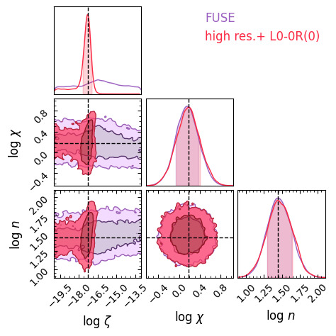
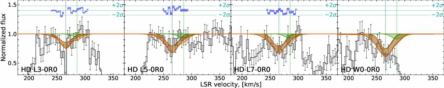
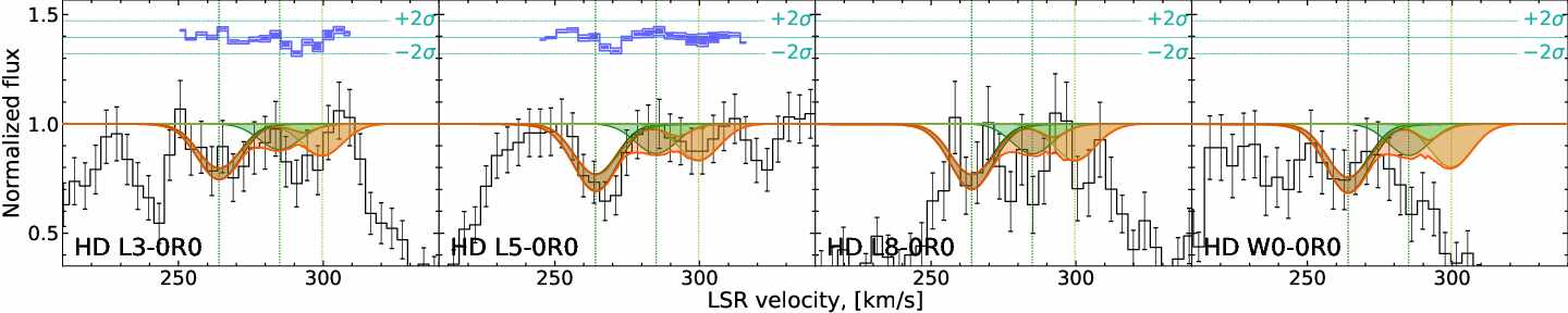
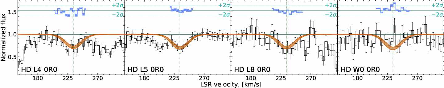
6 Discussion

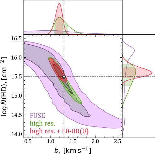
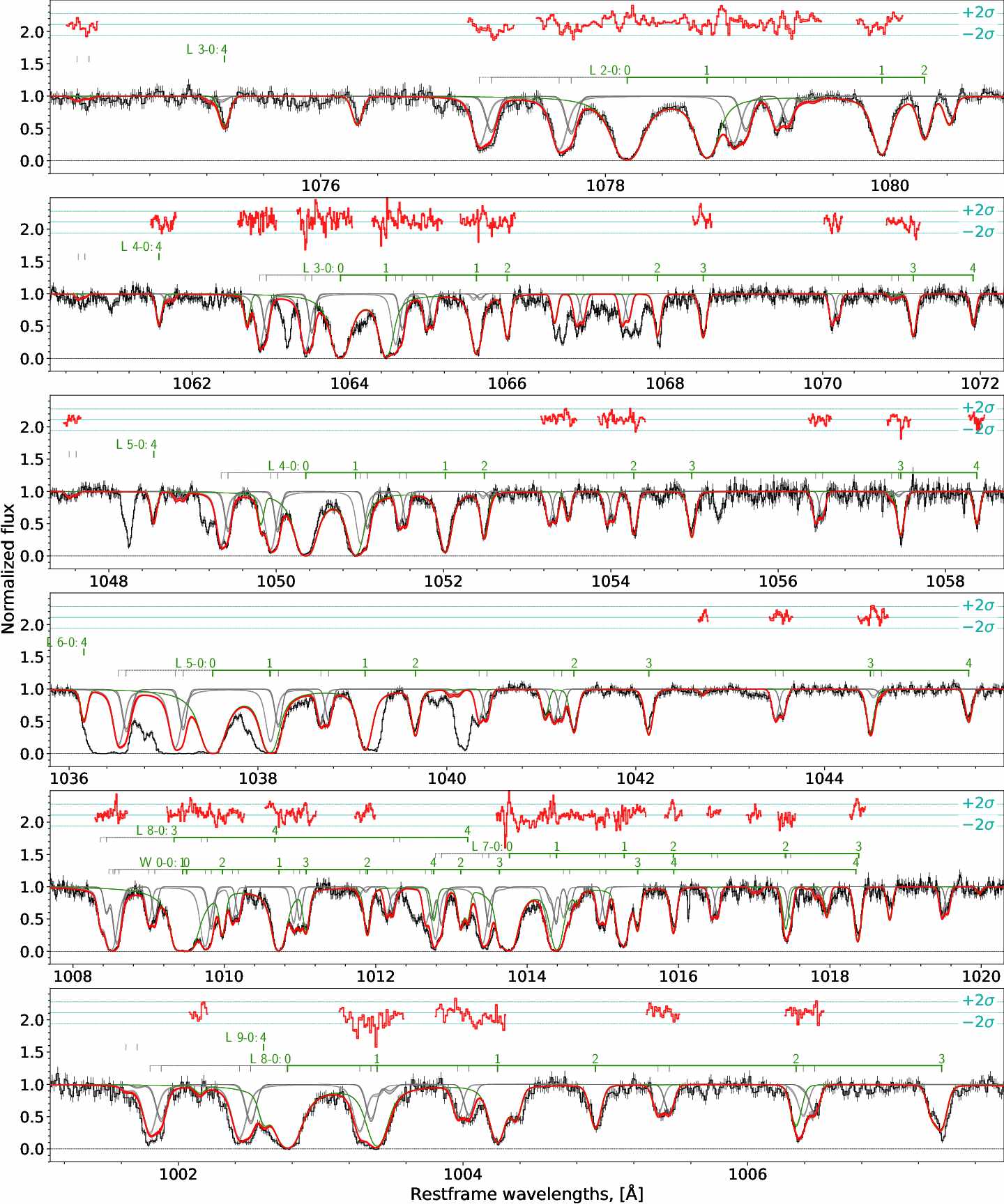
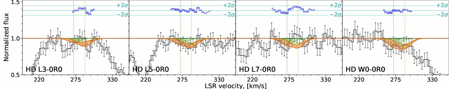
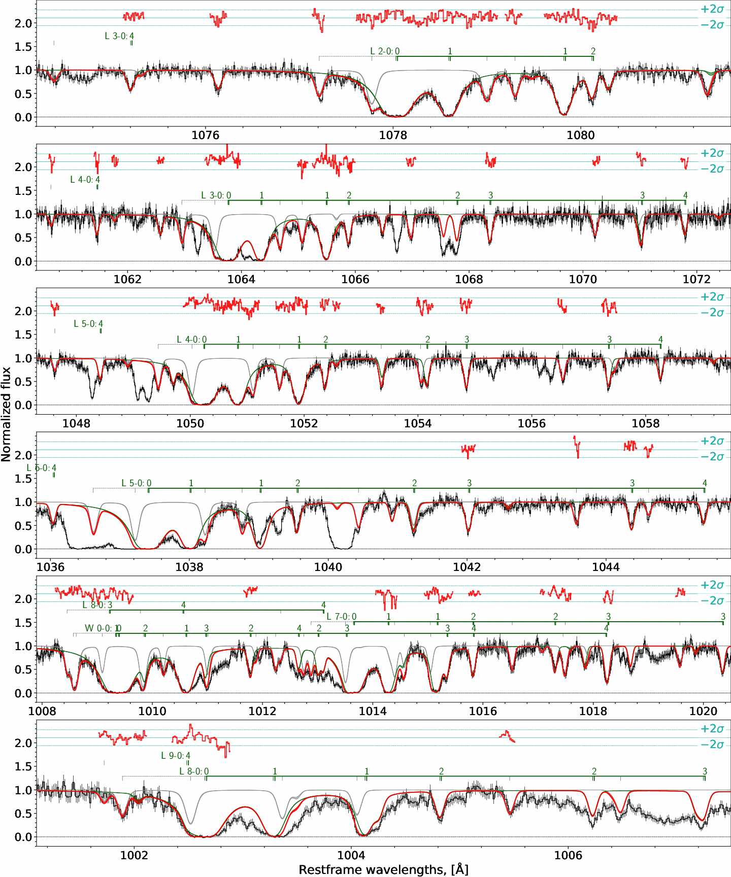
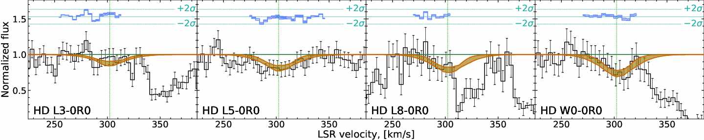
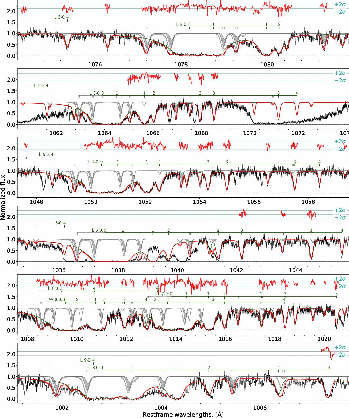
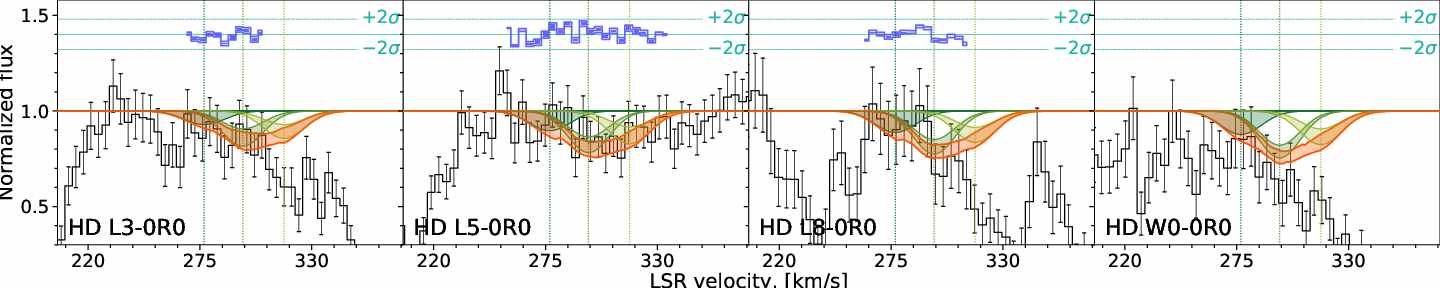
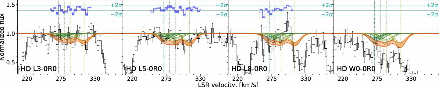
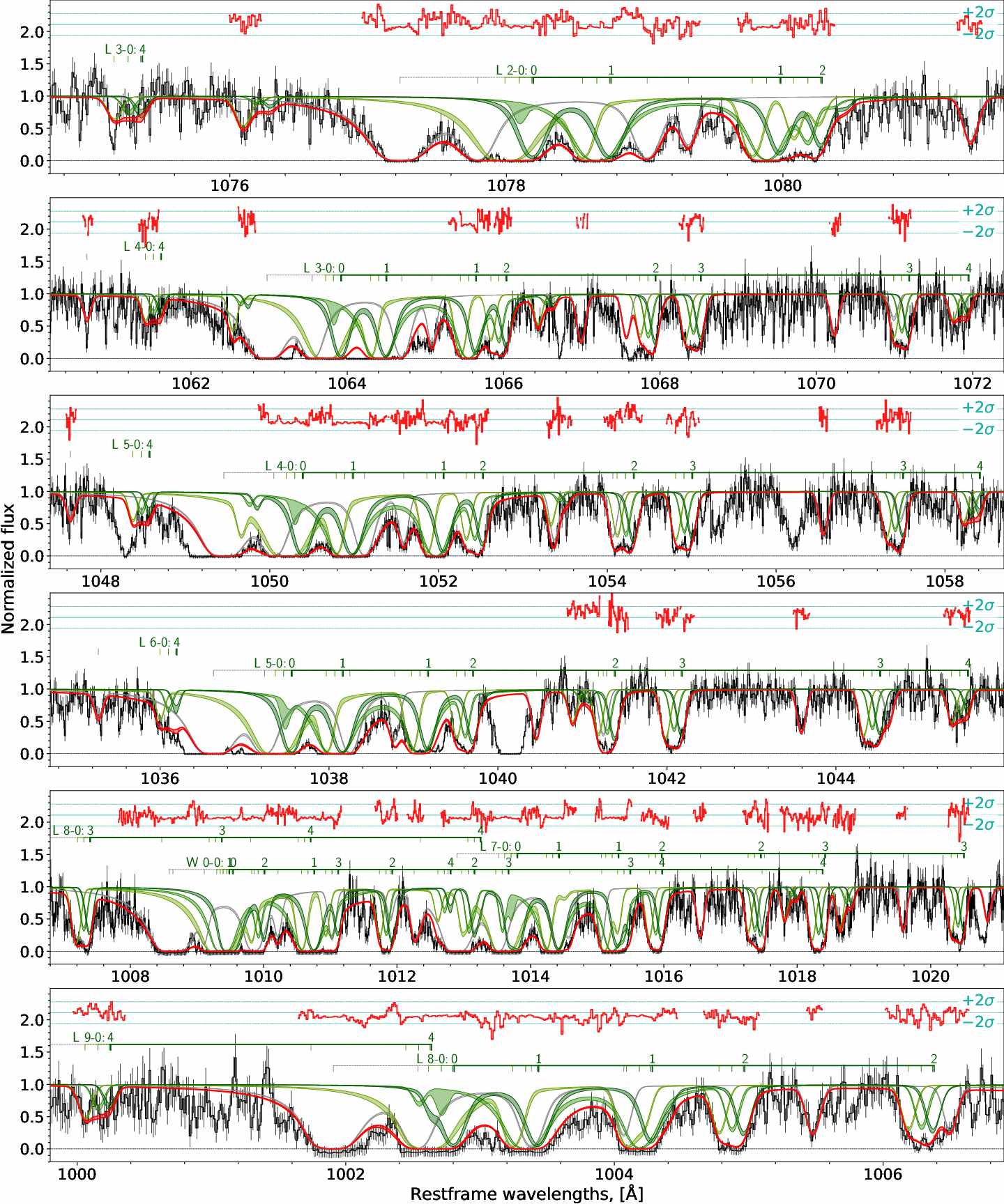
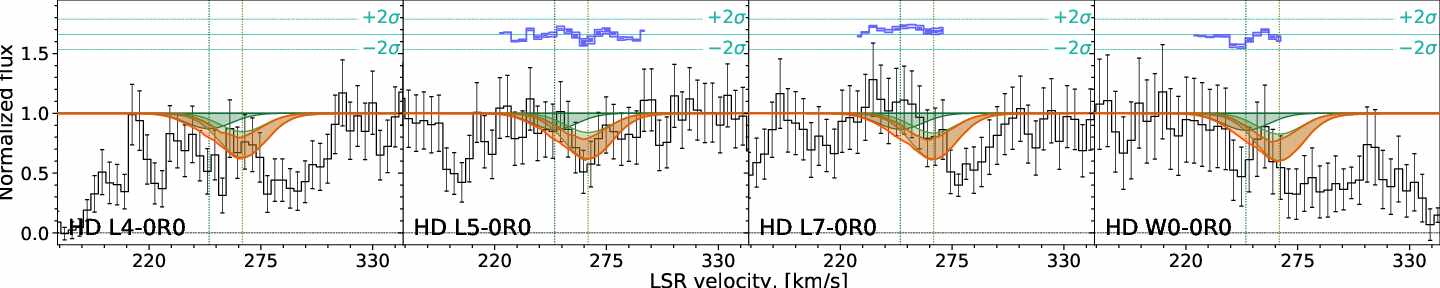
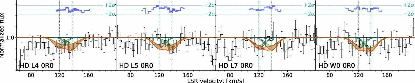
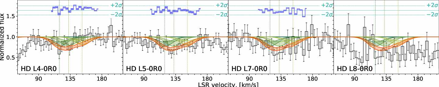
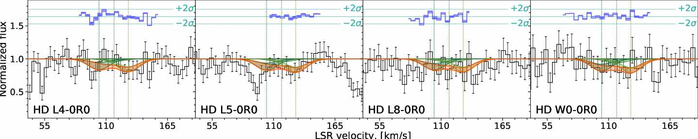
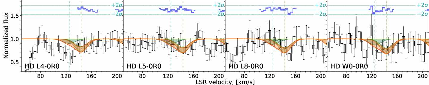
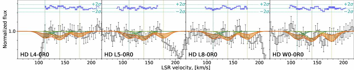
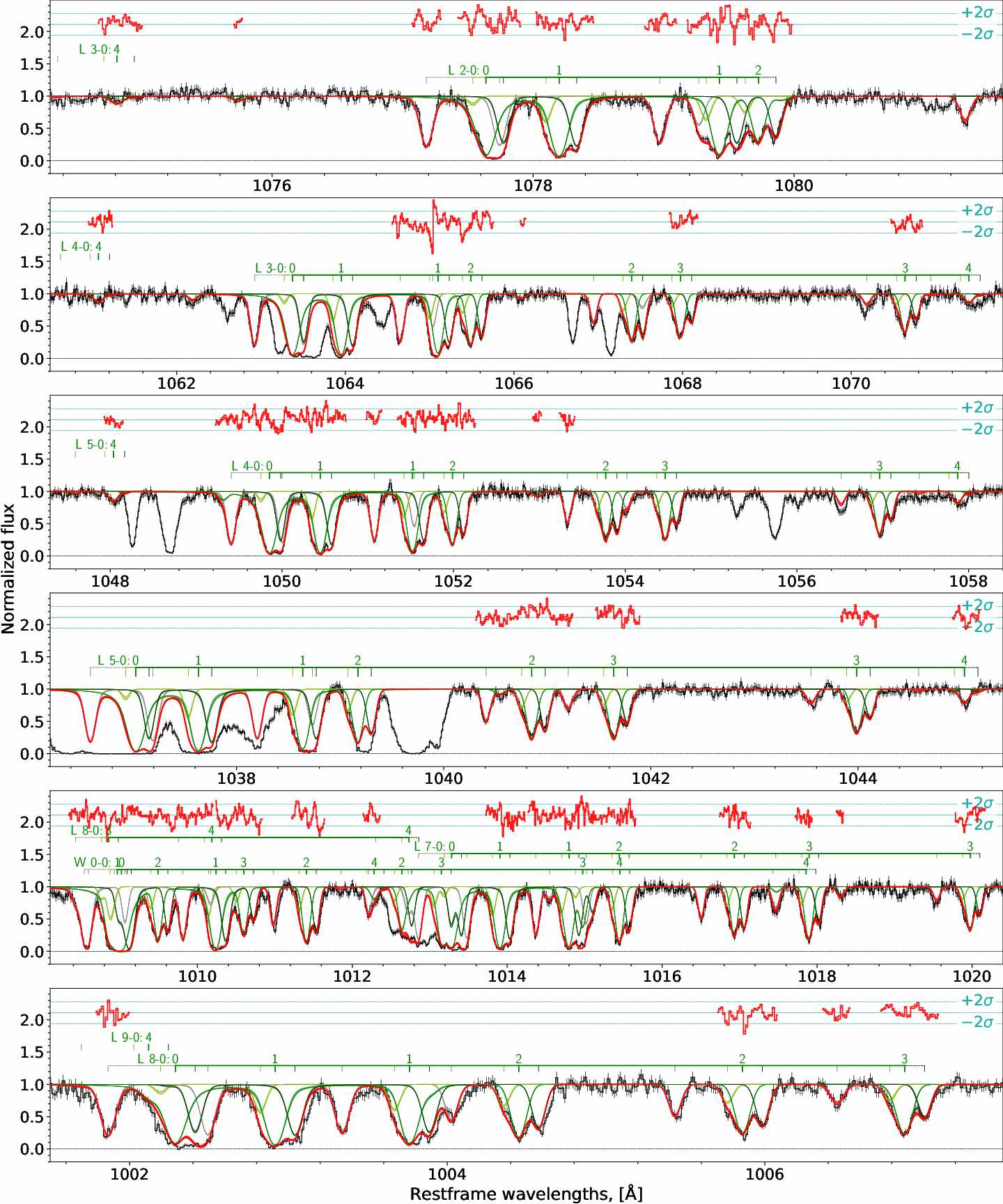
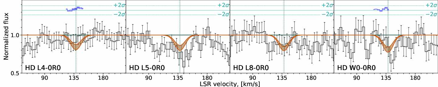
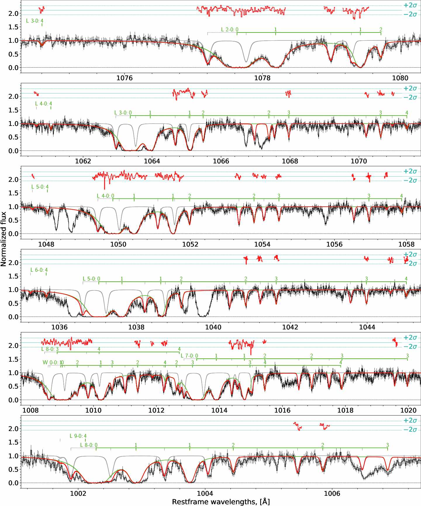
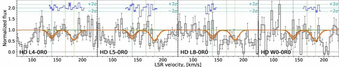
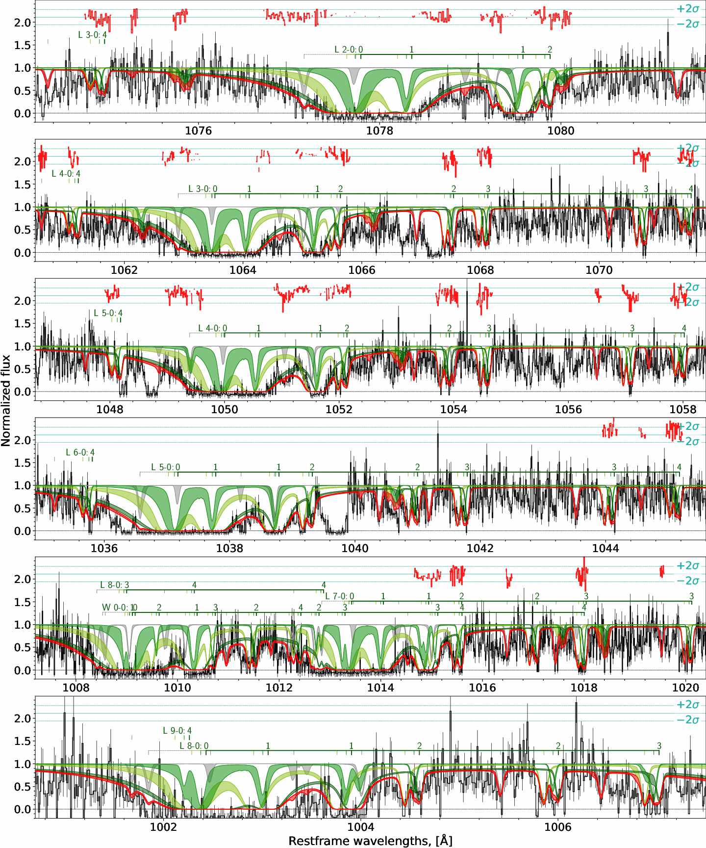
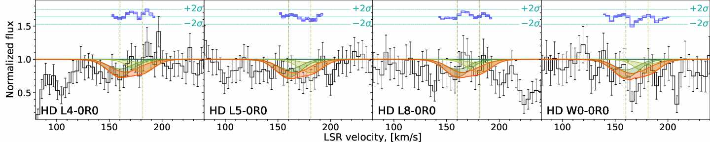
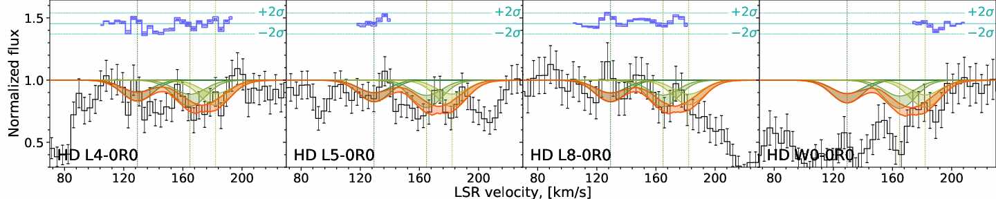
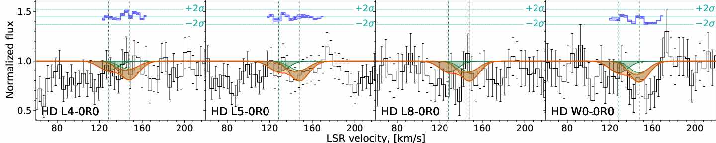
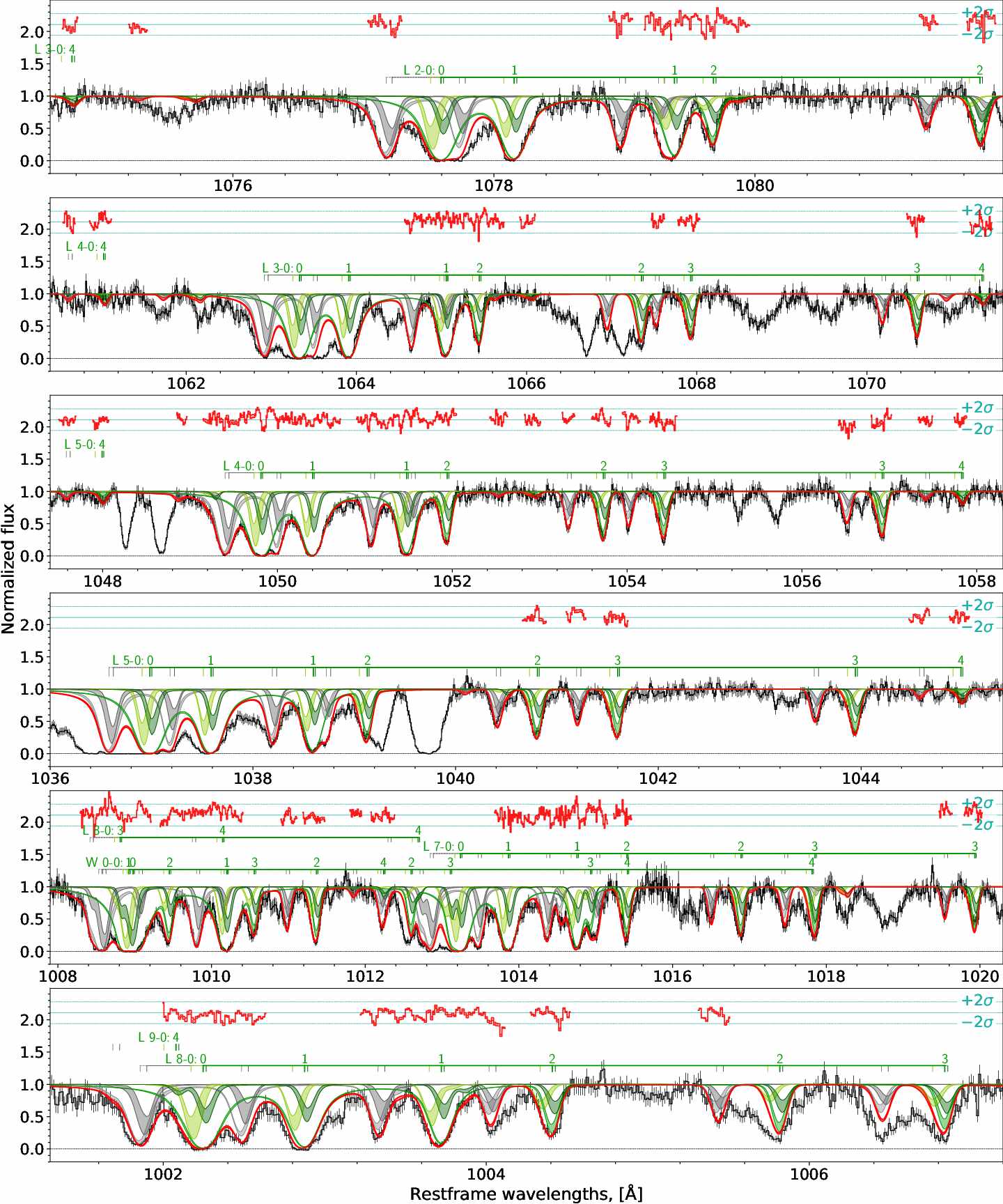
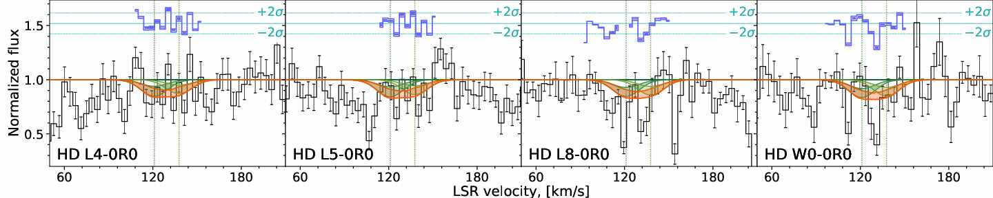
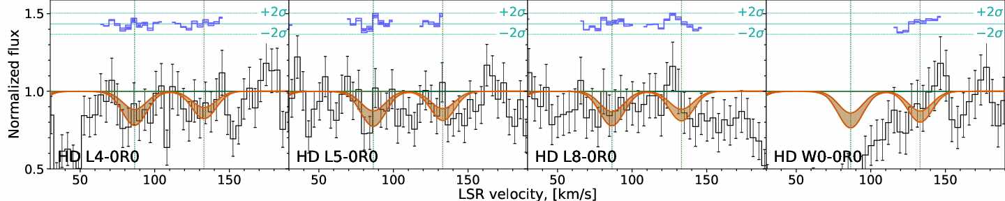
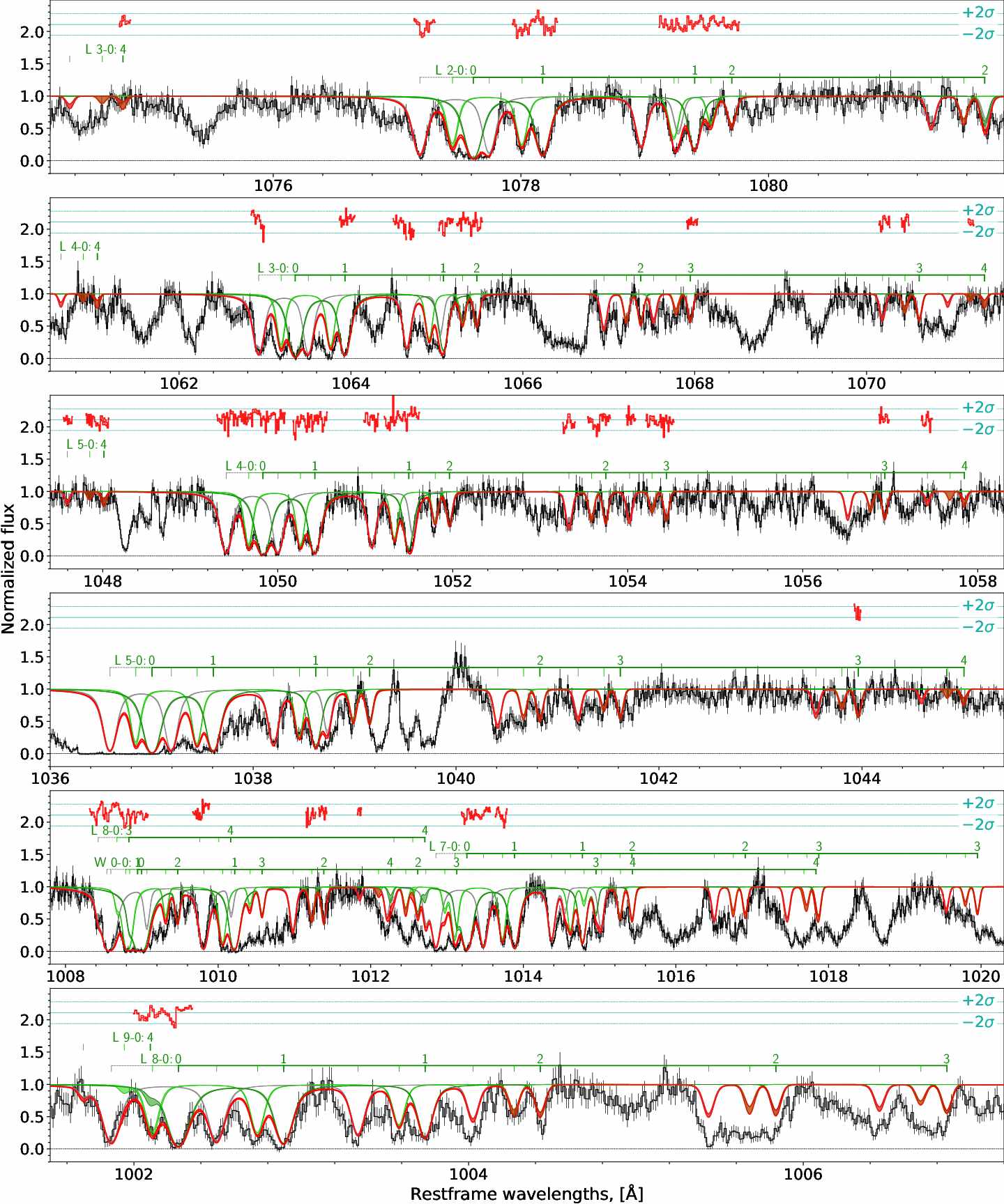
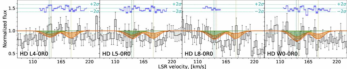
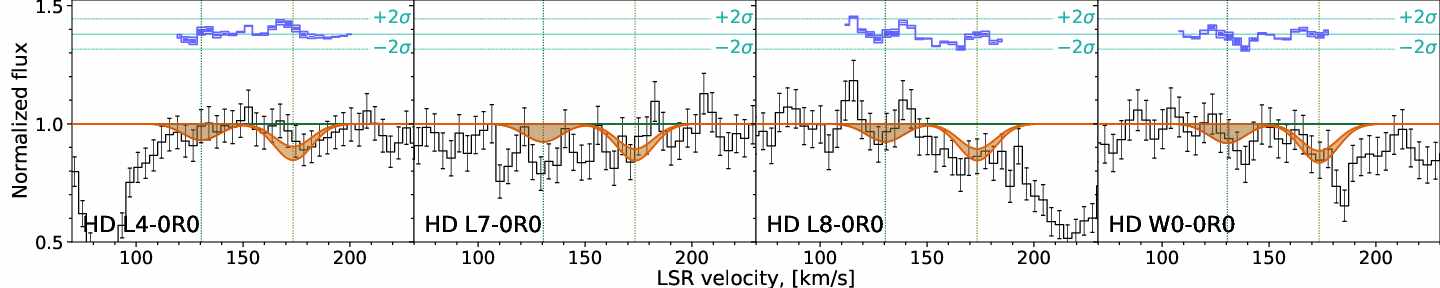
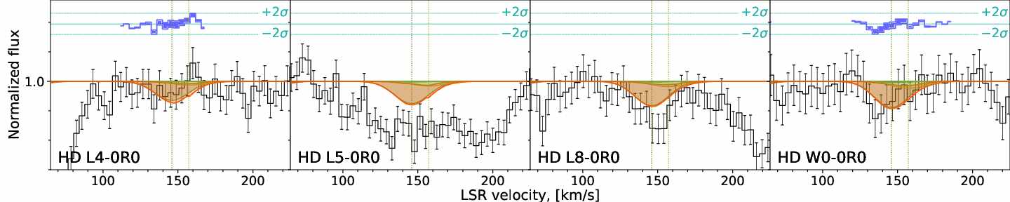
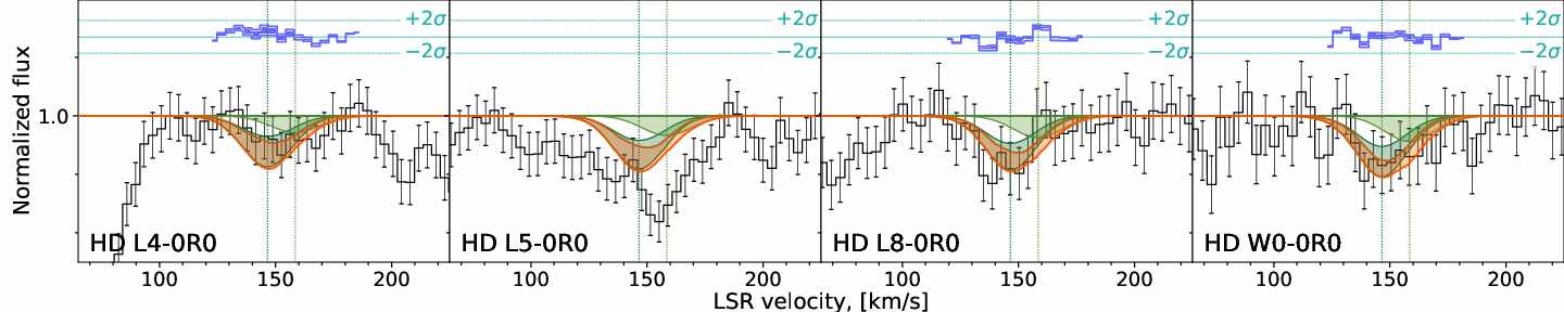
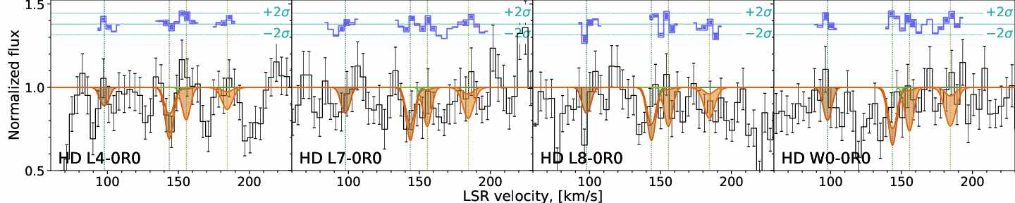
Nevertheless that we detected HD towards two dozens of LMC and SMC sightlines, we could not obtain reasonable constraint on CRIR using HD/H₂. The reason is that we get insufficient constraints on the HD column density due to low quality of the FUSE spectra. To illustrate this in Fig. 6 we compare line profiles and estimates of the fitting parameters of HD obtained from the FUSE spectra towards AV 490 and mock high resolution spectrum (with $R=50000$ and SNR=20). The original FUSE data indicates inability to remove degeneracy between high and low column density solutions, resulting in the wide ($\sim 2$ dex) constraint on the column density. One can see that the usage of the higher resolution not only allow to decompose the two velocity components in HD lines, but significantly reduces the constrained interval for HD column density. Moreover, the inclusion of the weakest HD line L0-0R(0) allows one to further shrink the interval and to get the uncertainties comparable to what is obtained for HD in high redshift DLAs Kosenko et al. 2021, see e.g.. This situation is similar to the case of the galactic sightlines, where HD measurement are also shallow, while typically galactic sightlines have higher SNR, which can reduce the uncertainty, but cannot remove the degeneracy. The lower uncertainty of HD column density will allow to get more strict constraints on CRIR, instead of upper limits obtained using FUSE real data, as is shown in the right panel of Fig. 6. Therefore, the next generation of the space UV telescopes, equipped with high resolution spectrograph will allow to constrain the CRIR using HD/H₂ ratio, that will provide important insights on the cold diffuse medium of the Magellanic clouds, as well as in our Galaxy.

Figure 6: Left: The profiles of selected HD lines. The blue and black lines show the real FUSE spectrum of AV 490 (shifted by 1 vertically for the presentation purposes) and the mock high resolution spectrum. To generate the mock spectrum we assume, that the $b=1.3\rm\,km\,s^{-1}$ and $\log N(\rm HD)=15.5$ (shown by cross at the middle panel). The fits to HD line profiles using two component Voigt function are shown by lavender, green and red lines and regions and correspond to FUSE (using L4-0R(0), L5-0R(0), L7-0R(0)), mock (the same sample of HD lines) and mock with additionally taking into account L0-0R(0) line, respectively. Middle: The 2d posterior in the Doppler parameter - column density space, obtained during the fit to HD lines. The color correspond to the fit shown in left panel. Right: The constraints on the CRIR using estimates of HD column density from FUSE spectrum (lavender lines and regions) and from high-resolution mock spectrum (red).

7 Summary

We have provided a systematic search for HD molecules in the LMC and SMC, the closest low-metallicity dwarf galaxies, using FUSE archival data. To make analysis homogeneous we reanalyzed H₂ using multicomponent Voight profile fitting of H₂ $\rm J\lesssim 5$ rotational levels. On the positions of H₂ components we looked for HD molecules. Although the quality of the FUSE data allows to obtain in the most cases only upper limits on HD column densities, we detected HD towards 24 sightlines (including 19 new detection).

In six systems (out of 24 where we have detected HD) we obtained constraints on CRIR, and in five among them we could place only upper limits, mostly due to large uncertainties in HD column density estimation. In the five systems we could not obtain reasonable constraints on the CRIR due to the too wide form of posterior probability functions, which cover all of the range within reasonable range of CRIR.

We also discuss influence of the spectral resolution on the results of our analysis and show that increase of the resolution of data will result in decrease of the column density uncertainties, which allows to obtain strict constraints on CRIR.

Data availability

The results of this paper are based on open data retrieved from the FUSE telescope archive. These data can be shared on reasonable requests to the authors.

Appendix A New HD detections

Figure 7: Fit to HD absorption lines towards LH10 3073 in LMC. Lines are the same as for 1.

Figure 8: Fit to HD absorption lines towards LH10 3102 in LMC. Lines are the same as for 1.

Figure 9: Fit to HD absorption lines towards Sk-70 79 in LMC. Lines are the same as for 1.

Figure 10: Fit to HD absorption lines towards Sk-68 73 in LMC. Lines are the same as for 1.

Figure 11: Fit to HD absorption lines towards Sk-71 46 in LMC. Lines are the same as for 1.

Figure 12: Fit to HD absorption lines towards J 0534-6932 in LMC. Lines are the same as for 1.

Figure 13: Fit to HD absorption lines towards BI 237 in LMC. Lines are the same as for 1.

Figure 14: Fit to HD absorption lines towards BI 253 in LMC. Lines are the same as for 1.

Figure 15: Fit to HD absorption lines towards Sk-68 137 in LMC. Lines are the same as for 1.

Figure 16: Fit to HD absorption lines towards AV 18 in SMC. Lines are the same as for 1.

Figure 17: Fit to HD absorption lines towards AV 26 in SMC. Lines are the same as for 1.

Figure 18: Fit to HD absorption lines towards AV 80 in SMC. Lines are the same as for 1.

Figure 19: Fit to HD absorption lines towards AV 208 in SMC. Lines are the same as for 1.

Figure 20: Fit to HD absorption lines towards AV 372 in SMC. Lines are the same as for 1.

Figure 21: Fit to HD absorption lines towards AV 435 in SMC. Lines are the same as for 1.

Figure 22: Fit to HD absorption lines towards AV 472 in SMC. Lines are the same as for 1.

Figure 23: Fit to HD absorption lines towards AV 486 in SMC. Lines are the same as for 1.

Figure 24: Fit to HD absorption lines towards AV 490 in SMC. Lines are the same as for 1.

Appendix B Detailed fitting results

B.1 Large Magellanic Cloud

Table 7: Fit results of H₂ lines towards Sk-67 2

species	comp	1	2	3
	z	$0.0000665(^{+25}_{-19})$	$0.000869(^{+3}_{-6})$	$0.000935(^{+6}_{-6})$
${\rm H_{2}\,J=0}$	b km/s	$0.91^{+0.72}_{-0.12}$	$0.81^{+0.14}_{-0.31}$	$0.98^{+0.23}_{-0.42}$
	$\log N$	$19.66^{+0.13}_{-0.09}$	$20.38^{+0.17}_{-0.65}$	$20.16^{+0.21}_{-0.43}$
${\rm H_{2}\,J=1}$	b km/s	$1.7^{+0.4}_{-0.8}$	$1.0^{+0.5}_{-0.4}$	$1.6^{+0.3}_{-0.4}$
	$\log N$	$19.4^{+0.4}_{-5.0}$	$19.64^{+0.14}_{-0.06}$	$20.01^{+0.10}_{-0.08}$
${\rm H_{2}\,J=2}$	b km/s	$4.4^{+0.3}_{-1.5}$	$2.0^{+0.5}_{-0.5}$	$1.82^{+0.45}_{-0.30}$
	$\log N$	$17.73^{+0.09}_{-0.47}$	$17.67^{+0.19}_{-0.23}$	$18.61^{+0.04}_{-0.17}$
${\rm H_{2}\,J=3}$	b km/s	$5.01^{+0.40}_{-0.31}$	$2.43^{+0.21}_{-0.35}$	$2.52^{+0.13}_{-0.41}$
	$\log N$	$15.87^{+0.42}_{-0.21}$	$17.65^{+0.09}_{-0.25}$	$17.29^{+0.14}_{-0.27}$
${\rm H_{2}\,J=4}$	$\log N$	$14.85^{+0.12}_{-0.14}$	$16.96^{+0.18}_{-0.72}$	$16.1^{+0.9}_{-0.3}$
	$\log N_{\rm tot}$	$19.84^{+0.19}_{-0.20}$	$20.46^{+0.15}_{-0.46}$	$20.40^{+0.14}_{-0.20}$
${\rm HD\,J=0}$	b km/s	$1.11^{+0.58}_{-0.29}$	$0.78^{+0.19}_{-0.15}$	$1.00^{+0.19}_{-0.34}$
	$\log N$	$\lesssim 16.9$	$\lesssim 17.1$	$\lesssim 17.3$

• Doppler parameters of H₂ ${\rm J=4}$ rotational levels were tied to H₂ ${\rm J=3}$.

  We have not fitted H₂ $\rm J>4$ lines due to low signal-to-noise ratio.

Figure 25: Fit to HD absorption lines towards Sk-67 2 in LMC. Here black line shows spectrum, red line represents obtained synthetic spectrum for HD. Green lines represent individual components. Regions between red and green lines were sampled from posterior probability distributions of fitting parameters. Blue points at the top of each panel show residuals. Here we show only components found in Magellanic Clouds.

Figure 26: Fit to H₂ absorption lines towards Sk-67 2 in LMC. Here black points with uncertainties show spectrum, red line represents total systhetic spectrum for H₂, grey lines show Milky Way subcomponents, green lines show Magellanic Cloud subcomponents. Regions between red, grey and green lines were sampled from posterior probability distributions of fitting parameters. Red points at the top of each panel show residuals.

Table 8: Fit results of H₂ lines towards Sk-67 5

species	comp	1	2
	z	$0.0000933(^{+12}_{-5})$	$0.00098317(^{+23}_{-34})$
${\rm H_{2}\,J=0}$	b km/s	$1.66^{+0.43}_{-0.19}$	$1.0^{+1.0}_{-0.5}$
	$\log N$	$15.6^{+0.3}_{-0.5}$	$19.315^{+0.004}_{-0.005}$
${\rm H_{2}\,J=1}$	b km/s	$5.01^{+0.34}_{-0.20}$	$4.65^{+0.24}_{-0.36}$
	$\log N$	$15.18^{+0.04}_{-0.06}$	$18.952^{+0.007}_{-0.005}$
${\rm H_{2}\,J=2}$	b km/s	$5.68^{+0.30}_{-0.72}$	$4.65^{+0.16}_{-0.27}$
	$\log N$	$14.395^{+0.037}_{-0.015}$	$16.88^{+0.14}_{-0.14}$
${\rm H_{2}\,J=3}$	b km/s	$6.08^{+0.26}_{-0.38}$	$4.51^{+0.18}_{-0.20}$
	$\log N$	$14.352^{+0.019}_{-0.034}$	$15.97^{+0.14}_{-0.09}$
${\rm H_{2}\,J=4}$	$\log N$	$13.20^{+0.11}_{-0.15}$	$14.644^{+0.036}_{-0.013}$
${\rm H_{2}\,J=5}$	$\log N$	$12.86^{+0.21}_{-0.32}$	$13.90^{+0.06}_{-0.07}$
	$\log N_{\rm tot}$	$15.81^{+0.23}_{-0.28}$	$19.473^{+0.003}_{-0.005}$
HD  J=0	b km/s	$9.81^{+0.19}_{-9.31}$	$0.31^{+1.77}_{-0.30}$
	$\log N_{\rm tot}$	$\lesssim 13.9$	$15.5^{+0.3}_{-2.1}$

• Doppler parameters of H₂ ${\rm J=4,5}$ rotational levels were tied to H₂ ${\rm J=3}$, while H₂ ${\rm J=1,2,3}$ were varied using penalty function.

Figure 27: Fit to HD absorption lines towards Sk-67 5 in LMC. Lines are the same as for 25.

Figure 28: Fit to H2 absorption lines towards Sk-67 5 in LMC. Lines are the same as for 26.

Table 9: Fit results of H₂ lines towards Sk-66 1

species	comp	1	2	3
	z	$-0.0000044(^{+20}_{-9})$	$0.0000860(^{+13}_{-8})$	$0.0009551(^{+11}_{-3})$
${\rm H_{2}\,J=0}$	b km/s	$0.94^{+1.56}_{-0.22}$	$7.3^{+0.4}_{-0.6}$	$1.6^{+1.1}_{-1.1}$
	$\log N$	$18.602^{+0.032}_{-0.030}$	$18.32^{+0.07}_{-0.06}$	$19.128^{+0.017}_{-0.006}$
${\rm H_{2}\,J=1}$	b km/s	$2.9^{+0.6}_{-1.3}$	$7.1^{+0.6}_{-0.6}$	$3.8^{+0.4}_{-2.5}$
	$\log N$	$18.922^{+0.029}_{-0.037}$	$17.21^{+0.47}_{-0.16}$	$18.875^{+0.026}_{-0.013}$
${\rm H_{2}\,J=2}$	b km/s	$3.1^{+0.4}_{-0.3}$	$6.8^{+0.6}_{-0.5}$	$4.6^{+0.5}_{-1.0}$
	$\log N$	$16.87^{+0.29}_{-0.31}$	$15.89^{+0.17}_{-0.17}$	$15.60^{+0.38}_{-0.26}$
${\rm H_{2}\,J=3}$	b km/s	$3.3^{+0.6}_{-0.5}$	$7.2^{+0.5}_{-0.6}$	$8.2^{+1.5}_{-0.9}$
	$\log N$	$15.5^{+0.4}_{-0.4}$	$15.50^{+0.15}_{-0.13}$	$14.93^{+0.05}_{-0.05}$
${\rm H_{2}\,J=4}$	b km/s	$5.6^{+2.5}_{-2.8}$	$7.3^{+1.2}_{-0.7}$	$9.89^{+4.24}_{-4.34}$
	$\log N$	$14.39^{+0.09}_{-0.07}$	$14.49^{+0.05}_{-0.05}$	$14.37^{+0.06}_{-0.06}$
	$\log N_{\rm tot}$	$19.09^{+0.02}_{-0.03}$	$18.35^{+0.08}_{-0.06}$	$19.32^{+0.01}_{-0.01}$
HD  J=0	b km/s	$0.73^{+1.11}_{-0.23}$	$7.3^{+0.5}_{-0.7}$	$0.57^{+1.65}_{-0.07}$
	$\log N$	$\lesssim 16.1$	$\lesssim 13.9$	$\lesssim 15.9$

Figure 29: Fit to HD absorption lines towards Sk-66 1 in LMC. Lines are the same as for 25.

Figure 30: Fit to H2 absorption lines towards Sk-66 1 in LMC. Lines are the same as for 26.

Table 10: Fit results of H₂ lines towards Sk-67 20

species	comp	1	2	3
	z	$-0.0000199(^{+7}_{-8})$	$0.0000597(^{+8}_{-12})$	$0.00094472(^{+26}_{-47})$
${\rm H_{2}\,J=0}$	b km/s	$1.8^{+0.4}_{-0.6}$	$2.08^{+0.38}_{-0.26}$	$1.6^{+0.6}_{-0.8}$
	$\log N$	$17.751^{+0.027}_{-0.048}$	$17.05^{+0.09}_{-0.18}$	$18.775^{+0.012}_{-0.006}$
${\rm H_{2}\,J=1}$	b km/s	$2.03^{+0.36}_{-0.22}$	$2.8^{+0.4}_{-0.3}$	$2.65^{+0.31}_{-0.21}$
	$\log N$	$18.120^{+0.024}_{-0.027}$	$16.89^{+0.24}_{-0.46}$	$18.642^{+0.007}_{-0.009}$
${\rm H_{2}\,J=2}$	b km/s	$2.10^{+0.17}_{-0.26}$	$3.5^{+0.4}_{-0.3}$	$2.76^{+0.15}_{-0.15}$
	$\log N$	$16.95^{+0.10}_{-0.18}$	$15.21^{+0.17}_{-0.16}$	$17.41^{+0.05}_{-0.04}$
${\rm H_{2}\,J=3}$	b km/s	$2.49^{+0.08}_{-0.08}$	$3.77^{+0.55}_{-0.25}$	$2.73^{+0.11}_{-0.24}$
	$\log N$	$16.26^{+0.11}_{-0.11}$	$14.92^{+0.09}_{-0.08}$	$17.40^{+0.07}_{-0.06}$
${\rm H_{2}\,J=4}$	b km/s	–	$4.3^{+0.5}_{-0.5}$	$2.76^{+0.19}_{-0.16}$
	$\log N$	$13.96^{+0.06}_{-0.09}$	$13.71^{+0.11}_{-0.11}$	$15.98^{+0.16}_{-0.12}$
${\rm H_{2}\,J=5}$	b km/s	–	–	$3.59^{+0.11}_{-0.30}$
	$\log N$	$13.95^{+0.07}_{-0.15}$	$13.88^{+0.12}_{-0.10}$	$15.26^{+0.11}_{-0.11}$
${\rm H_{2}\,J=6}$	$\log N$	–	–	$13.74^{+0.06}_{-0.09}$
	$\log N_{\rm tot}$	$18.30^{+0.02}_{-0.02}$	$17.28^{+0.12}_{-0.17}$	$19.036^{+0.007}_{-0.006}$
${\rm HD\,J=0}$	b km/s	$0.527^{+1.279}_{-0.027}$	$2.05^{+0.45}_{-0.28}$	$0.53^{+1.08}_{-0.03}$
	$\log N$	$\lesssim 15.3$	$\lesssim 13.9$	$\lesssim 14.2$

• Doppler parameters of H₂ ${\rm J=4,5}$ rotational levels in the 1 component, H₂ $J=5$ in the 2 component and H₂ $J=6$ in the 3 component were tied to H₂ ${\rm J=3}$.

Figure 31: Fit to HD absorption lines towards Sk-67 20 in LMC. Lines are the same as for 25.

Figure 32: Fit to H2 absorption lines towards Sk-67 20 in LMC. Lines are the same as for 26.

Table 11: Fit results of H₂ lines towards Sk-66 18

species	comp	1	2	3	4
	z	$0.0000084(^{+14}_{-10})$	$0.0000945(^{+8}_{-7})$	$0.0009155(^{+20}_{-31})$	$0.0009712(^{+31}_{-23})$
${\rm H_{2}\,J=0}$	b km/s	$2.29^{+0.19}_{-0.16}$	$2.8^{+0.9}_{-0.5}$	$2.9^{+0.3}_{-0.6}$	$0.73^{+0.47}_{-0.23}$
	$\log N$	$14.91^{+0.11}_{-0.14}$	$17.70^{+0.08}_{-0.16}$	$17.18^{+0.18}_{-0.17}$	$17.91^{+0.07}_{-0.05}$
${\rm H_{2}\,J=1}$	b km/s	$2.69^{+0.16}_{-0.13}$	$3.89^{+0.21}_{-0.28}$	$3.10^{+0.36}_{-0.27}$	$1.1^{+0.5}_{-0.3}$
	$\log N$	$16.10^{+0.13}_{-0.11}$	$17.57^{+0.16}_{-0.04}$	$17.53^{+0.13}_{-0.17}$	$17.82^{+0.07}_{-0.09}$
${\rm H_{2}\,J=2}$	b km/s	$2.15^{+0.16}_{-0.07}$	$4.03^{+0.31}_{-0.26}$	$3.2^{+0.4}_{-0.4}$	$3.5^{+0.7}_{-1.0}$
	$\log N$	$16.60^{+0.12}_{-0.11}$	$16.32^{+0.17}_{-0.28}$	$15.82^{+0.22}_{-0.30}$	$15.05^{+0.25}_{-0.14}$
${\rm H_{2}\,J=3}$	b km/s	$3.6^{+5.0}_{-0.9}$	$4.20^{+0.56}_{-0.30}$	$3.35^{+0.29}_{-0.50}$	$8.5^{+2.5}_{-5.0}$
	$\log N$	$14.59^{+0.06}_{-0.06}$	$15.48^{+0.13}_{-0.23}$	$15.24^{+0.11}_{-0.19}$	$14.73^{+0.06}_{-0.08}$
${\rm H_{2}\,J=4}$	b km/s	–	–	$10.7^{+5.3}_{-3.0}$	$11.1^{+4.7}_{-2.4}$
	$\log N$	$13.78^{+0.10}_{-0.20}$	$14.351^{+0.067}_{-0.022}$	$14.03^{+0.16}_{-0.06}$	$13.88^{+0.10}_{-0.13}$
${\rm H_{2}\,J=5}$	$\log N$	–	–	$13.62^{+0.17}_{-0.22}$	$13.77^{+0.13}_{-0.16}$
	$\log N_{\rm tot}$	$16.73^{+0.10}_{-0.08}$	$17.95^{+0.08}_{-0.08}$	$17.70^{+0.11}_{-0.12}$	$18.17^{+0.05}_{-0.05}$
HD  J=0	b km/s	$2.28^{+0.21}_{-0.17}$	$2.7^{+1.1}_{-0.5}$	$2.98^{+0.28}_{-0.72}$	$0.522^{+0.388}_{-0.022}$
	$\log N$	$\lesssim 13.9$	$\lesssim 13.6$	$\lesssim 14.0$	$\lesssim 15.7$

• Doppler parameters of H₂ ${\rm J=4}$ rotational levels in the 1 and 2 components, H₂ $J=5$ in the 3 and 4 components were tied to H₂ ${\rm J=3}$ and ${\rm J=4}$, respectively.

Figure 33: Fit to HD absorption lines towards Sk-66 18 in LMC. Lines are the same as for 25.

Figure 34: Fit to H2 absorption lines towards Sk-66 18 in LMC. Lines are the same as for 26.

Table 12: Fit results of H₂ lines towards PGMW 3070

species	comp	1	2	3	4
	z	$-0.0000121(^{+5}_{-12})$	$0.0000680(^{+9}_{-6})$	$0.0008822(^{+13}_{-3})$	$0.0009555(^{+7}_{-5})$
${\rm H_{2}\,J=0}$	b km/s	$1.0^{+0.5}_{-0.4}$	$1.35^{+0.31}_{-0.70}$	$0.62^{+0.30}_{-0.08}$	$0.69^{+0.47}_{-0.15}$
	$\log N$	$18.686^{+0.032}_{-0.015}$	$18.053^{+0.020}_{-0.051}$	$17.67^{+0.09}_{-0.11}$	$18.950^{+0.028}_{-0.007}$
${\rm H_{2}\,J=1}$	b km/s	$1.7^{+0.6}_{-0.8}$	$2.87^{+0.21}_{-1.06}$	$1.13^{+0.35}_{-0.27}$	$1.72^{+0.08}_{-0.91}$
	$\log N$	$18.604^{+0.030}_{-0.022}$	$18.40^{+0.03}_{-0.04}$	$17.922^{+0.041}_{-0.030}$	$18.592^{+0.013}_{-0.017}$
${\rm H_{2}\,J=2}$	b km/s	$2.75^{+0.18}_{-0.20}$	$2.85^{+0.13}_{-0.19}$	$2.32^{+0.17}_{-0.20}$	$1.91^{+0.22}_{-0.25}$
	$\log N$	$17.57^{+0.09}_{-0.06}$	$17.41^{+0.05}_{-0.14}$	$16.73^{+0.18}_{-0.18}$	$17.512^{+0.030}_{-0.070}$
${\rm H_{2}\,J=3}$	b km/s	$2.69^{+0.24}_{-0.21}$	$3.25^{+0.10}_{-0.26}$	$2.57^{+0.58}_{-0.21}$	$2.18^{+0.30}_{-0.16}$
	$\log N$	$16.99^{+0.18}_{-0.21}$	$16.74^{+0.24}_{-0.10}$	$15.86^{+0.24}_{-0.49}$	$17.23^{+0.09}_{-0.12}$
${\rm H_{2}\,J=4}$	b km/s	$3.3^{+0.6}_{-0.6}$	$5.2^{+0.8}_{-1.3}$	$3.1^{+0.9}_{-0.7}$	$2.42^{+0.39}_{-0.31}$
	$\log N$	$14.56^{+0.07}_{-0.08}$	$14.48^{+0.05}_{-0.04}$	$13.92^{+0.05}_{-0.16}$	$15.50^{+0.15}_{-0.53}$
${\rm H_{2}\,J=5}$	b km/s	$4.8^{+1.3}_{-0.6}$	$18.0^{+1.9}_{-5.7}$	$3.6^{+1.1}_{-0.9}$	$2.6^{+1.1}_{-0.4}$
	$\log N$	$14.21^{+0.04}_{-0.10}$	$12.4^{+0.6}_{-0.9}$	$14.044^{+0.097}_{-0.021}$	$14.41^{+0.10}_{-0.07}$
	$\log N_{\rm tot}$	$19.97^{+0.02}_{-0.01}$	$18.60^{+0.02}_{-0.03}$	$18.14^{+0.04}_{-0.04}$	$19.124^{+0.019}_{-0.007}$
HD  J=0	b km/s	$0.525^{+0.587}_{-0.025}$	$0.522^{+0.876}_{-0.022}$	$0.62^{+0.25}_{-0.12}$	$0.71^{+0.30}_{-0.20}$
	$\log N$	$\lesssim 15.9$	$\lesssim 15.5$	$\lesssim 15.6$	$\lesssim 16.0$

Figure 35: Fit to HD absorption lines towards PGMW 3070 in LMC. Lines are the same as for 25.

Figure 36: Fit to H2 absorption lines towards PGMW 3070 in LMC. Lines are the same as for 26.

Table 13: Fit results of H₂ lines towards LH10 3073

species	comp	1	2	3	4
	z	$-0.0000064(^{+15}_{-16})$	$0.0000763(^{+10}_{-21})$	$0.0008855(^{+18}_{-9})$	$0.0009532(^{+18}_{-18})$
${\rm H_{2}\,J=0}$	b km/s	$0.57^{+0.06}_{-0.06}$	$0.518^{+0.052}_{-0.018}$	$0.85^{+0.11}_{-0.31}$	$0.74^{+0.35}_{-0.17}$
	$\log N$	$19.108^{+0.024}_{-0.025}$	$18.28^{+0.09}_{-0.05}$	$19.006^{+0.013}_{-0.046}$	$17.4^{+0.5}_{-3.7}$
${\rm H_{2}\,J=1}$	b km/s	$0.60^{+0.07}_{-0.09}$	$0.578^{+0.026}_{-0.063}$	$1.01^{+0.18}_{-0.28}$	$1.05^{+0.27}_{-0.31}$
	$\log N$	$18.953^{+0.023}_{-0.029}$	$18.28^{+0.06}_{-0.09}$	$18.859^{+0.022}_{-0.022}$	$17.87^{+0.05}_{-0.13}$
${\rm H_{2}\,J=2}$	b km/s	$0.69^{+0.09}_{-0.11}$	$0.587^{+0.076}_{-0.028}$	$1.24^{+0.15}_{-0.30}$	$1.55^{+0.07}_{-0.33}$
	$\log N$	$18.139^{+0.015}_{-0.043}$	$17.62^{+0.04}_{-0.05}$	$17.750^{+0.045}_{-0.029}$	$16.96^{+0.13}_{-0.11}$
${\rm H_{2}\,J=3}$	b km/s	$0.825^{+0.030}_{-0.158}$	$0.65^{+0.04}_{-0.05}$	$1.35^{+0.11}_{-0.24}$	$1.59^{+0.08}_{-0.07}$
	$\log N$	$17.94^{+0.03}_{-0.04}$	$17.62^{+0.04}_{-0.04}$	$17.72^{+0.03}_{-0.05}$	$16.64^{+0.16}_{-0.13}$
${\rm H_{2}\,J=4}$	b km/s	$0.85^{+0.05}_{-0.08}$	$0.687^{+0.025}_{-0.070}$	$1.37^{+0.14}_{-0.12}$	–
	$\log N$	$16.75^{+0.06}_{-0.12}$	$16.20^{+0.10}_{-0.15}$	$16.24^{+0.16}_{-0.15}$	$14.72^{+0.16}_{-0.26}$
${\rm H_{2}\,J=5}$	$\log N$	$16.20^{+0.22}_{-0.26}$	$15.37^{+0.39}_{-0.31}$	$15.24^{+0.43}_{-0.25}$	$12.8^{+0.3}_{-0.3}$
	$\log N_{\rm tot}$	$19.38^{+0.02}_{-0.02}$	$18.67^{+0.05}_{-0.04}$	$19.27^{+0.01}_{-0.03}$	$18.05^{+0.17}_{-0.14}$
HD  J=0	b km/s	$0.59^{+0.05}_{-0.06}$	$0.505^{+0.073}_{-0.005}$	$2.5^{+11.5}_{-2.0}$	$0.81^{+0.15}_{-0.10}$
	$\log N_{\rm tot}$	$\lesssim 16.4$	$\lesssim 16.0$	$14.3^{+0.9}_{-0.3}$	$\lesssim 15.3$

• Doppler parameters of H₂ ${\rm J=5}$ rotational levels were tied to H₂ ${\rm J=4}$, Doppler parameter of H₂ ${\rm J=4}$ was tied to H₂ ${\rm J=3}$.

Figure 37: Fit to HD absorption lines towards LH10 3073 in LMC. Lines are the same as for 25.

Figure 38: Fit to H2 absorption lines towardsLH10 3073 in LMC. Lines are the same as for 26.

Table 14: Fit results of H₂ lines towards LH10 3102

species	comp	1	2	3	4	5	6	7	8
	z	$-0.0001336(^{+37}_{-22})$	$-0.0000657(^{+34}_{-7})$	$0.0000039(^{+11}_{-7})$	$0.0000772(^{+9}_{-13})$	$0.0001332(^{+7}_{-32})$	$0.0008807(^{+20}_{-9})$	$0.0009506(^{+10}_{-12})$	$0.0009996(^{+3}_{-15})$
${\rm H_{2}\,J=0}$	b km/s	$0.64^{+0.49}_{-0.12}$	$0.92^{+0.44}_{-0.20}$	$1.49^{+0.61}_{-0.29}$	$0.518^{+0.155}_{-0.018}$	$1.8^{+1.0}_{-0.5}$	$0.73^{+0.18}_{-0.17}$	$0.61^{+0.25}_{-0.09}$	$1.8^{+0.7}_{-0.7}$
	$\log N$	$13.0^{+0.4}_{-0.4}$	$15.27^{+0.68}_{-0.25}$	$18.79^{+0.04}_{-0.04}$	$17.95^{+0.09}_{-0.09}$	$13.06^{+0.21}_{-0.24}$	$16.99^{+0.09}_{-0.19}$	$18.428^{+0.050}_{-0.025}$	$12.90^{+0.13}_{-0.18}$
${\rm H_{2}\,J=1}$	b km/s	$1.23^{+0.69}_{-0.30}$	$1.32^{+0.25}_{-0.40}$	$2.06^{+0.19}_{-0.31}$	$0.68^{+0.29}_{-0.11}$	$2.7^{+0.4}_{-0.6}$	$1.68^{+0.25}_{-0.11}$	$0.92^{+0.32}_{-0.25}$	$2.6^{+0.8}_{-0.9}$
	$\log N$	$14.44^{+0.35}_{-0.22}$	$15.61^{+0.43}_{-0.26}$	$18.594^{+0.077}_{-0.017}$	$17.96^{+0.07}_{-0.07}$	$14.27^{+0.16}_{-0.29}$	$17.35^{+0.15}_{-0.06}$	$18.166^{+0.018}_{-0.078}$	$13.85^{+0.13}_{-0.19}$
${\rm H_{2}\,J=2}$	b km/s	$1.8^{+0.4}_{-0.7}$	$2.62^{+0.21}_{-0.55}$	$2.36^{+0.12}_{-0.31}$	$2.48^{+0.29}_{-0.16}$	$3.15^{+0.28}_{-0.50}$	$2.05^{+0.21}_{-0.21}$	$2.52^{+0.20}_{-0.19}$	$4.7^{+0.5}_{-1.0}$
	$\log N$	$13.45^{+0.11}_{-1.12}$	$14.56^{+0.13}_{-0.13}$	$17.77^{+0.08}_{-0.05}$	$16.59^{+0.14}_{-0.31}$	$14.67^{+0.14}_{-0.19}$	$15.65^{+0.29}_{-0.09}$	$16.39^{+0.16}_{-0.15}$	$14.27^{+0.11}_{-0.08}$
${\rm H_{2}\,J=3}$	b km/s	$2.8^{+0.3}_{-0.3}$	$4.1^{+0.6}_{-0.4}$	$2.45^{+0.21}_{-0.29}$	$4.27^{+0.26}_{-0.61}$	$2.91^{+0.44}_{-0.29}$	$2.55^{+0.31}_{-0.48}$	$2.92^{+0.19}_{-0.37}$	$4.9^{+0.5}_{-1.0}$
	$\log N$	$14.06^{+0.12}_{-1.12}$	$14.35^{+0.08}_{-0.11}$	$17.44^{+0.14}_{-0.11}$	$15.25^{+0.32}_{-0.13}$	$14.27^{+0.08}_{-0.12}$	$14.85^{+0.27}_{-0.14}$	$15.38^{+0.24}_{-0.12}$	$14.13^{+0.12}_{-0.06}$
${\rm H_{2}\,J=4}$	b km/s	$3.9^{+0.5}_{-0.4}$	$5.4^{+0.4}_{-0.6}$	$2.20^{+0.21}_{-0.26}$	–	–	–	–	–
	$\log N$	$13.91^{+0.09}_{-0.21}$	$12.39^{+0.72}_{-0.22}$	$15.57^{+0.18}_{-0.51}$	$14.24^{+0.07}_{-0.10}$	$13.77^{+0.13}_{-0.40}$	$13.63^{+0.21}_{-0.23}$	$14.14^{+0.08}_{-0.15}$	$13.66^{+0.16}_{-0.27}$
${\rm H_{2}\,J=5}$	b km/s	–	–	$4.82^{+0.14}_{-0.07}$	–	–	–	–	–
	$\log N$	–	–	$13.933^{+0.021}_{-0.044}$	–	–	–	–	–
	$\log N_{\rm tot}$	$14.71^{+0.22}_{-0.16}$	$15.82^{+0.40}_{-0.16}$	$19.04^{+0.04}_{-0.02}$	$18.26^{+0.06}_{-0.05}$	$14.96^{+0.09}_{-0.11}$	$17.51^{+0.11}_{-0.06}$	$18.62^{+0.03}_{-0.03}$	$14.65^{+0.07}_{-0.05}$
HD  J=0	b km/s	$0.81^{+0.43}_{-0.30}$	$0.84^{+0.48}_{-0.25}$	$1.3^{+0.8}_{-0.4}$	$0.63^{+0.12}_{-0.10}$	$1.6^{+1.4}_{-0.5}$	$0.50^{+4.23}_{-0.00}$	$0.67^{+0.17}_{-0.16}$	$1.6^{+1.1}_{-0.5}$
	$\log N$	$\lesssim 15.3$	$\lesssim 15.6$	$\lesssim 15.8$	$\lesssim 15.6$	$\lesssim 15.8$	$14.15^{+0.46}_{-0.28}$	$\lesssim 15.6$	$\lesssim 15.7$

• Doppler parameters of H₂ ${\rm J=4}$ rotational levels in 4, 5, 6, 7 and 8 components were tied to H₂ ${\rm J=3}$.

Figure 39: Fit to HD absorption lines towards LH10 3102 in LMC. Lines are the same as for 25.

Figure 40: Fit to H2 absorption lines towards LH10 3102 in LMC. Lines are the same as for 26.

Table 15: Fit results of H₂ lines towards LH10 3120

species	comp	1	2	3	4
	z	$-0.0000008(^{+5}_{-7})$	$0.0000846(^{+5}_{-7})$	$0.0009079(^{+20}_{-8})$	$0.0009645(^{+15}_{-9})$
${\rm H_{2}\,J=0}$	b km/s	$0.54^{+0.38}_{-0.04}$	$2.3^{+0.5}_{-0.7}$	$2.57^{+0.29}_{-0.77}$	$0.58^{+0.40}_{-0.08}$
	$\log N$	$18.392^{+0.032}_{-0.031}$	$18.350^{+0.032}_{-0.022}$	$17.86^{+0.04}_{-0.07}$	$17.40^{+0.05}_{-0.09}$
${\rm H_{2}\,J=1}$	b km/s	$0.88^{+0.26}_{-0.34}$	$2.4^{+0.5}_{-0.6}$	$3.12^{+0.15}_{-0.09}$	$2.10^{+0.19}_{-0.32}$
	$\log N$	$18.562^{+0.028}_{-0.013}$	$18.499^{+0.017}_{-0.032}$	$17.97^{+0.05}_{-0.05}$	$17.71^{+0.10}_{-0.06}$
${\rm H_{2}\,J=2}$	b km/s	$2.91^{+0.16}_{-0.12}$	$3.88^{+0.17}_{-0.18}$	$3.10^{+0.13}_{-0.13}$	$3.02^{+0.11}_{-0.13}$
	$\log N$	$17.73^{+0.04}_{-0.04}$	$17.25^{+0.11}_{-0.14}$	$15.46^{+0.11}_{-0.23}$	$16.38^{+0.39}_{-0.08}$
${\rm H_{2}\,J=3}$	b km/s	$3.29^{+0.16}_{-0.18}$	$4.51^{+0.23}_{-0.23}$	$3.15^{+0.13}_{-0.09}$	$3.32^{+0.16}_{-0.08}$
	$\log N$	$17.36^{+0.08}_{-0.11}$	$16.28^{+0.14}_{-0.17}$	$14.73^{+0.07}_{-0.07}$	$16.05^{+0.17}_{-0.12}$
${\rm H_{2}\,J=4}$	b km/s	$3.47^{+0.52}_{-0.25}$	$5.06^{+0.26}_{-0.26}$	–	–
	$\log N$	$15.26^{+0.26}_{-0.16}$	$14.03^{+0.19}_{-0.24}$	$13.45^{+0.21}_{-0.20}$	$14.21^{+0.11}_{-0.09}$
${\rm H_{2}\,J=5}$	b km/s	–	–	–	–
	$\log N$	$14.68^{+0.13}_{-0.09}$	$13.85^{+0.19}_{-0.39}$	$13.83^{+0.13}_{-0.14}$	$12.9^{+0.4}_{-0.3}$
	$\log N_{\rm tot}$	$18.84^{+0.02}_{-0.01}$	$18.75^{+0.02}_{-0.02}$	$18.22^{+0.03}_{-0.04}$	$17.90^{+0.07}_{-0.05}$
HD  J=0	b km/s	$0.518^{+0.374}_{-0.018}$	$2.4^{+0.5}_{-0.9}$	$2.66^{+0.31}_{-0.90}$	$0.522^{+0.507}_{-0.022}$
	$\log N$	$\lesssim 16.1$	$\lesssim 15.5$	$\lesssim 15.3$	$\lesssim 15.4$

• Doppler parameters of H₂ ${\rm J=5}$ rotational level in component 1 and 2 and ${\rm J=4,5}$ in components 3 and 4 were tied to H₂ ${\rm J=4}$ and ${\rm J=3}$, respectively.

Figure 41: Fit to HD absorption lines towards LH10 3120 in LMC. Lines are the same as for 25.

Figure 42: Fit to H2 absorption lines towards LH10 3120 in LMC. Lines are the same as for 26.

Table 16: Fit results of H₂ lines towards PGMW 3157

species	comp	1	2	3	4	5
	z	$-0.0000029(^{+11}_{-37})$	$0.0000745(^{+40}_{-22})$	$0.000122(^{+4}_{-5})$	$0.0008904(^{+54}_{-29})$	$0.0009579(^{+20}_{-40})$
${\rm H_{2}\,J=0}$	b km/s	$0.71^{+0.67}_{-0.12}$	$1.0^{+0.6}_{-0.4}$	$0.78^{+0.82}_{-0.26}$	$0.9^{+0.6}_{-0.4}$	$3.2^{+1.5}_{-0.9}$
	$\log N$	$16.82^{+0.18}_{-0.46}$	$18.38^{+0.08}_{-0.12}$	$17.3^{+0.4}_{-0.6}$	$16.9^{+0.4}_{-0.5}$	$18.85^{+0.05}_{-0.03}$
${\rm H_{2}\,J=1}$	b km/s	$1.50^{+0.73}_{-0.21}$	$2.3^{+0.6}_{-0.6}$	$1.7^{+0.4}_{-0.8}$	$2.6^{+0.7}_{-0.7}$	$4.3^{+0.9}_{-0.7}$
	$\log N$	$17.10^{+0.20}_{-0.37}$	$18.52^{+0.06}_{-0.07}$	$15.7^{+0.7}_{-0.5}$	$17.15^{+0.29}_{-0.82}$	$18.76^{+0.04}_{-0.06}$
${\rm H_{2}\,J=2}$	b km/s	$3.8^{+0.5}_{-0.5}$	$2.8^{+0.7}_{-0.4}$	$4.0^{+0.5}_{-1.7}$	$2.8^{+0.8}_{-0.5}$	$5.3^{+0.6}_{-0.6}$
	$\log N$	$15.93^{+0.31}_{-0.35}$	$17.16^{+0.29}_{-0.49}$	$14.43^{+0.23}_{-0.16}$	$15.64^{+0.22}_{-0.63}$	$17.54^{+0.33}_{-0.14}$
${\rm H_{2}\,J=3}$	b km/s	$4.6^{+0.4}_{-0.7}$	$4.4^{+0.5}_{-0.6}$	$4.9^{+0.4}_{-2.0}$	$3.5^{+1.1}_{-1.0}$	$6.0^{+1.9}_{-0.6}$
	$\log N$	$15.40^{+0.30}_{-0.16}$	$16.61^{+0.10}_{-0.61}$	$14.2^{+0.3}_{-0.3}$	$14.82^{+0.23}_{-0.25}$	$17.09^{+0.21}_{-0.61}$
${\rm H_{2}\,J=4}$	b km/s	–	–	–	–	$10.5^{+2.2}_{-3.3}$
	$\log N$	$14.30^{+0.09}_{-0.14}$	$14.53^{+0.09}_{-0.11}$	$13.68^{+0.30}_{-2.11}$	$14.05^{+0.16}_{-0.23}$	$14.83^{+0.04}_{-0.08}$
${\rm H_{2}\,J=5}$	$\log N$	$14.17^{+0.15}_{-0.24}$	$13.6^{+0.5}_{-0.7}$	$13.9^{+0.3}_{-3.0}$	$14.39^{+0.17}_{-0.18}$	$14.54^{+0.09}_{-0.09}$
	$\log N_{\rm tot}$	$17.30^{+0.15}_{-0.23}$	$18.77^{+0.05}_{-0.06}$	$17.31^{+0.39}_{-0.57}$	$17.35^{+0.25}_{-0.38}$	$19.13^{+0.03}_{-0.03}$
HD J=0	b km/s	$0.88^{+0.44}_{-0.25}$	$1.0^{+0.5}_{-0.4}$	$0.79^{+0.53}_{-0.29}$	$1.1^{+0.4}_{-0.4}$	$2.6^{+1.9}_{-1.2}$
	$\log N$	$\lesssim 16.6$	$\lesssim 16.4$	$\lesssim 16.4$	$\lesssim 16.5$	$\lesssim 16.5$

• Doppler parameters of H₂ ${\rm J=4,5}$ rotational levels in 1, 2, 3 and 4 components and H₂ ${\rm J=5}$ in 5 components were tied to H₂ ${\rm J=3}$ and ${\rm J=4}$, respectively.

Figure 43: Fit to HD absorption lines towards PGMW 3157 in LMC. Lines are the same as for 25.

Figure 44: Fit to H2 absorption lines towards PGMW 3157 in LMC. Lines are the same as for 26.

Table 17: Fit results of H₂ lines towards PGMW 3223

species	comp	1	2	3	4
	z	$-0.0000170(^{+6}_{-14})$	$0.0000652(^{+9}_{-7})$	$0.0008933(^{+8}_{-7})$	$0.0009599(^{+18}_{-30})$
${\rm H_{2}\,J=0}$	b km/s	$1.5^{+1.4}_{-0.3}$	$2.49^{+0.23}_{-0.62}$	$0.68^{+0.26}_{-0.16}$	$0.53^{+0.21}_{-0.03}$
	$\log N$	$16.71^{+0.20}_{-0.37}$	$17.57^{+0.04}_{-0.07}$	$18.561^{+0.021}_{-0.016}$	$14.8^{+0.4}_{-0.8}$
${\rm H_{2}\,J=1}$	b km/s	$2.29^{+1.84}_{-0.25}$	$2.79^{+0.30}_{-0.34}$	$1.2^{+0.8}_{-0.4}$	$1.23^{+0.64}_{-0.24}$
	$\log N$	$15.60^{+0.58}_{-0.18}$	$17.86^{+0.06}_{-0.06}$	$18.378^{+0.024}_{-0.023}$	$14.73^{+0.32}_{-0.14}$
${\rm H_{2}\,J=2}$	b km/s	$6.19^{+0.31}_{-0.62}$	$5.3^{+0.3}_{-0.7}$	$3.8^{+0.5}_{-0.5}$	$2.7^{+0.3}_{-0.5}$
	$\log N$	$14.82^{+0.03}_{-0.04}$	$15.13^{+0.14}_{-0.07}$	$15.54^{+0.38}_{-0.18}$	$14.24^{+0.08}_{-0.11}$
${\rm H_{2}\,J=3}$	b km/s	$6.3^{+0.4}_{-0.4}$	$5.7^{+0.3}_{-0.3}$	$7.9^{+0.8}_{-1.0}$	$2.93^{+0.18}_{-0.26}$
	$\log N$	$14.718^{+0.026}_{-0.039}$	$14.742^{+0.035}_{-0.031}$	$15.03^{+0.03}_{-0.04}$	$14.57^{+0.04}_{-0.12}$
${\rm H_{2}\,J=4}$	b km/s	–	–	$8.7^{+0.5}_{-1.4}$	–
	$\log N$	$13.91^{+0.10}_{-0.15}$	$13.96^{+0.09}_{-0.13}$	$14.39^{+0.05}_{-0.04}$	$13.86^{+0.15}_{-0.11}$
	$\log N_{\rm tot}$	$16.75^{+0.19}_{-0.32}$	$18.04^{+0.04}_{-0.05}$	$18.78^{+0.02}_{-0.01}$	$15.27^{+0.22}_{-0.17}$
HD  J=0	b km/s	$1.5^{+1.8}_{-0.4}$	$2.51^{+0.28}_{-0.72}$	$0.514^{+0.336}_{-0.014}$	$0.510^{+0.225}_{-0.010}$
	$\log N$	$\lesssim 14.5$	$\lesssim 15.2$	$\lesssim 15.9$	$\lesssim 15.7$

• Doppler parameters of H₂ ${\rm J=4}$ rotational levels in 1, 2 and 4 components were tied to H₂ ${\rm J=3}$.

• Resolution was fixed to be $R=18000$

Figure 45: Fit to HD absorption lines towards PGMW 3223 in LMC. Lines are the same as for 25.

Figure 46: Fit to H2 absorption lines towards PGMW 3223 in LMC. Lines are the same as for 26.

Table 18: Fit results of H₂ lines towards Sk-66 35

species	comp	1	2	3	4	5
	z	$-0.0000192(^{+21}_{-14})$	$0.0000730(^{+8}_{-8})$	$0.000882(^{+10}_{-10})$	$0.0009186(^{+15}_{-14})$	$0.000954(^{+9}_{-4})$
${\rm H_{2}\,J=0}$	b km/s	$1.84^{+0.29}_{-0.24}$	$1.5^{+0.5}_{-0.9}$	$0.68^{+0.98}_{-0.18}$	$0.73^{+0.76}_{-0.22}$	$0.9^{+0.6}_{-0.3}$
	$\log N$	$15.24^{+0.34}_{-0.20}$	$17.827^{+0.041}_{-0.031}$	$18.22^{+0.27}_{-0.23}$	$18.85^{+0.19}_{-0.06}$	$18.61^{+0.19}_{-0.14}$
${\rm H_{2}\,J=1}$	b km/s	$1.99^{+0.26}_{-0.33}$	$2.5^{+0.5}_{-0.8}$	$0.68^{+1.50}_{-0.18}$	$0.77^{+0.76}_{-0.18}$	$1.3^{+0.6}_{-0.6}$
	$\log N$	$17.11^{+0.12}_{-0.29}$	$18.17^{+0.04}_{-0.05}$	$17.70^{+0.40}_{-0.25}$	$19.124^{+0.019}_{-0.021}$	$17.47^{+0.31}_{-0.89}$
${\rm H_{2}\,J=2}$	b km/s	$3.3^{+0.4}_{-0.8}$	$3.53^{+0.46}_{-0.21}$	$0.79^{+1.94}_{-0.29}$	$1.6^{+0.4}_{-0.7}$	$1.5^{+0.8}_{-0.5}$
	$\log N$	$15.10^{+0.25}_{-0.21}$	$17.28^{+0.09}_{-0.35}$	$14.4^{+1.4}_{-0.3}$	$18.142^{+0.029}_{-0.081}$	$14.8^{+0.9}_{-0.3}$
${\rm H_{2}\,J=3}$	b km/s	$4.0^{+1.1}_{-0.7}$	$3.36^{+1.13}_{-0.20}$	$0.90^{+2.71}_{-0.23}$	$1.7^{+0.5}_{-0.6}$	$7.39^{+5.58}_{-5.94}$
	$\log N$	$14.56^{+0.08}_{-0.08}$	$16.64^{+0.21}_{-0.65}$	$13.1^{+1.2}_{-0.8}$	$17.73^{+0.06}_{-0.13}$	$14.20^{+0.30}_{-0.21}$
${\rm H_{2}\,J=4}$	b km/s	–	–	$4.6^{+3.9}_{-2.1}$	$3.05^{+0.40}_{-0.22}$	–
	$\log N$	$13.04^{+0.31}_{-0.58}$	$14.12^{+0.09}_{-0.16}$	$10.29^{+2.13}_{-0.27}$	$16.01^{+0.10}_{-0.39}$	$12.9^{+0.7}_{-1.2}$
${\rm H_{2}\,J=5}$	$\log N$	–	–	$10.5^{+1.5}_{-0.5}$	$14.59^{+0.10}_{-0.11}$	–
	$\log N_{\rm tot}$	$17.13^{+0.12}_{-0.28}$	$18.38^{+0.03}_{-0.04}$	$18.34^{+0.24}_{-0.18}$	$19.35^{+0.07}_{-0.02}$	$18.64^{+0.18}_{-0.13}$
HD  J=0	b km/s	$1.80^{+0.37}_{-0.28}$	$0.530^{+1.180}_{-0.030}$	$0.55^{+1.07}_{-0.05}$	$0.54^{+1.03}_{-0.04}$	$0.80^{+0.70}_{-0.30}$
	$\log N$	$\lesssim 14.5$	$\lesssim 16.1$	$\lesssim 16.2$	$\lesssim 15.9$	$\lesssim 15.7$

• Doppler parameters of H₂ ${\rm J=4}$ rotational levels in 1, 2 and 5 components were tied to H₂ ${\rm J=3}$.

Figure 47: Fit to HD absorption lines towards Sk-66 35 in LMC. Lines are the same as for 25.

Figure 48: Fit to H2 absorption lines towards Sk-66 35 in LMC. Lines are the same as for 26.

Table 19: Fit results of H₂ lines towards Sk-69 52

species	comp	1	2
	z	$0.0000808(^{+9}_{-8})$	$0.0008653(^{+12}_{-10})$
${\rm H_{2}\,J=0}$	b km/s	$0.526^{+0.429}_{-0.026}$	$0.506^{+0.171}_{-0.006}$
	$\log N$	$18.454^{+0.026}_{-0.020}$	$18.452^{+0.038}_{-0.021}$
${\rm H_{2}\,J=1}$	b km/s	$0.77^{+0.43}_{-0.25}$	$0.63^{+0.13}_{-0.13}$
	$\log N$	$18.487^{+0.023}_{-0.021}$	$18.158^{+0.026}_{-0.026}$
${\rm H_{2}\,J=2}$	b km/s	$1.04^{+0.61}_{-0.16}$	$0.79^{+0.14}_{-0.17}$
	$\log N$	$17.63^{+0.04}_{-0.07}$	$16.70^{+0.08}_{-0.16}$
${\rm H_{2}\,J=3}$	b km/s	$1.60^{+0.12}_{-0.53}$	$0.99^{+0.08}_{-0.16}$
	$\log N$	$17.09^{+0.14}_{-0.11}$	$15.98^{+0.35}_{-0.27}$
${\rm H_{2}\,J=4}$	$\log N$	$14.9^{+0.6}_{-0.4}$	$14.7^{+0.6}_{-0.3}$
	$\log N_{\rm tot}$	$18.81^{+0.02}_{-0.01}$	$18.64^{+0.02}_{-0.02}$
HD  J=0	b km/s	$0.519^{+0.419}_{-0.019}$	$0.508^{+0.171}_{-0.008}$
	$\log N$	$\lesssim 16.3$	$\lesssim 15.6$

• Doppler parameters of H₂ ${\rm J=4}$ rotational levels in both components were tied to H₂ ${\rm J=3}$.

Figure 49: Fit to HD absorption lines towards Sk-69 52 in LMC. Lines are the same as for 25.

Figure 50: Fit to H2 absorption lines towards Sk-69 52 in LMC. Lines are the same as for 26.

Table 20: Fit results of H₂ lines towards Sk-65 21

species	comp	1	2
	z	$0.00010030(^{+14}_{-27})$	$0.00082643(^{+26}_{-34})$
${\rm H_{2}\,J=0}$	b km/s	$2.63^{+0.12}_{-0.06}$	$1.5^{+0.6}_{-0.5}$
	$\log N$	$17.646^{+0.008}_{-0.020}$	$17.969^{+0.014}_{-0.012}$
${\rm H_{2}\,J=1}$	b km/s	$2.28^{+0.09}_{-0.09}$	$2.00^{+0.21}_{-0.45}$
	$\log N$	$17.978^{+0.007}_{-0.014}$	$18.147^{+0.009}_{-0.015}$
${\rm H_{2}\,J=2}$	b km/s	$2.34^{+0.27}_{-0.20}$	$2.48^{+0.06}_{-0.12}$
	$\log N$	$17.23^{+0.12}_{-0.14}$	$16.93^{+0.07}_{-0.04}$
${\rm H_{2}\,J=3}$	b km/s	$4.99^{+0.32}_{-0.23}$	$3.34^{+0.17}_{-0.06}$
	$\log N$	$15.26^{+0.10}_{-0.04}$	$15.50^{+0.04}_{-0.04}$
${\rm H_{2}\,J=4}$	b km/s	$6.2^{+0.8}_{-0.9}$	$3.36^{+0.19}_{-0.18}$
	$\log N$	$14.342^{+0.020}_{-0.015}$	$14.07^{+0.04}_{-0.05}$
${\rm H_{2}\,J=5}$	b km/s	$6.6^{+1.7}_{-1.0}$	–
	$\log N$	$13.918^{+0.026}_{-0.038}$	$13.71^{+0.08}_{-0.09}$
	$\log N_{\rm tot}$	$18.19^{+0.02}_{-0.02}$	$18.38^{+0.01}_{-0.01}$
HD J=0	b km/s	$2.62^{+0.15}_{-0.06}$	$0.530^{+0.413}_{-0.030}$
	$\log N$	$\lesssim 13.6$	$\lesssim 15.9$

• Doppler parameter of H₂ ${\rm J=5}$ rotational levels in the 2 component was tied to H₂ ${\rm J=4}$.

Figure 51: Fit to HD absorption lines towards Sk-65 21 in LMC. Lines are the same as for 25.

Figure 52: Fit to H2 absorption lines towards Sk-65 21 in LMC. Lines are the same as for 26.

Table 21: Fit results of H₂ lines towards Sk-66 51

species	comp	1	2
	z	$0.0000861(^{+3}_{-10})$	$0.0010389(^{+8}_{-7})$
${\rm H_{2}\,J=0}$	b km/s	$2.6^{+0.3}_{-0.3}$	$0.70^{+0.22}_{-0.20}$
	$\log N$	$16.99^{+0.11}_{-0.18}$	$17.854^{+0.026}_{-0.026}$
${\rm H_{2}\,J=1}$	b km/s	$2.89^{+0.22}_{-0.21}$	$1.01^{+0.25}_{-0.34}$
	$\log N$	$17.32^{+0.10}_{-0.09}$	$17.656^{+0.026}_{-0.020}$
${\rm H_{2}\,J=2}$	b km/s	$2.84^{+0.37}_{-0.16}$	$1.41^{+0.28}_{-0.15}$
	$\log N$	$15.95^{+0.12}_{-0.32}$	$16.46^{+0.14}_{-0.27}$
${\rm H_{2}\,J=3}$	b km/s	$8.3^{+0.6}_{-0.9}$	$1.58^{+0.19}_{-0.15}$
	$\log N$	$14.539^{+0.028}_{-0.028}$	$15.56^{+0.28}_{-0.24}$
${\rm H_{2}\,J=4}$	$\log N$	$13.62^{+0.20}_{-0.23}$	$13.88^{+0.16}_{-0.22}$
	$\log N_{\rm tot}$	$17.50^{+0.08}_{-0.08}$	$18.08^{+0.02}_{-0.02}$
HD J=0	b km/s	$2.64^{+0.28}_{-0.37}$	$0.511^{+0.345}_{-0.011}$
	$\log N$	$\lesssim 14.2$	$\lesssim 15.3$

• Doppler parameters of H₂ ${\rm J=4}$ rotational levels were tied to H₂ ${\rm J=3}$.

Figure 53: Fit to HD absorption lines towards Sk-66 51 in LMC. Lines are the same as for 25.

Figure 54: Fit to H2 absorption lines towards Sk-66 51 in LMC. Lines are the same as for 26.

Table 22: Fit results of H₂ lines towards Sk-70 79

species	comp	1	2
	z	$0.0000214(^{+11}_{-9})$	$0.0007824(^{+4}_{-3})$
${\rm H_{2}\,J=0}$	b km/s	$1.03^{+0.22}_{-0.32}$	$0.59^{+0.51}_{-0.08}$
	$\log N$	$17.792^{+0.025}_{-0.025}$	$20.1386^{+0.0049}_{-0.0017}$
${\rm H_{2}\,J=1}$	b km/s	$1.28^{+0.09}_{-0.26}$	$0.95^{+0.31}_{-0.37}$
	$\log N$	$16.10^{+0.17}_{-0.10}$	$19.9712^{+0.0048}_{-0.0013}$
${\rm H_{2}\,J=2}$	b km/s	$4.65^{+0.26}_{-0.25}$	$1.0^{+0.4}_{-0.4}$
	$\log N$	$15.20^{+0.11}_{-0.07}$	$18.768^{+0.005}_{-0.009}$
${\rm H_{2}\,J=3}$	b km/s	$4.50^{+0.19}_{-0.25}$	$4.88^{+0.23}_{-0.35}$
	$\log N$	$14.716^{+0.085}_{-0.021}$	$17.53^{+0.11}_{-0.09}$
${\rm H_{2}\,J=4}$	b km/s	–	$5.48^{+0.26}_{-0.33}$
	$\log N$	$13.3^{+0.4}_{-0.3}$	$16.04^{+0.16}_{-0.11}$
${\rm H_{2}\,J=5}$	b km/s	–	$5.1^{+0.4}_{-0.4}$
	$\log N$	–	$15.12^{+0.16}_{-0.04}$
${\rm H_{2}\,J=6}$	b km/s	–	$5.8^{+3.3}_{-1.0}$
	$\log N$	–	$14.17^{+0.06}_{-0.07}$
	$\log N_{\rm tot}$	$17.80^{+0.02}_{-0.03}$	$20.375^{+0.003}_{-0.002}$
HD J=0	b km/s	$1.00^{+0.17}_{-0.28}$	$2.0^{+0.7}_{-0.6}$
	$\log N$	$\lesssim 16.1$	$15.6^{+0.7}_{-0.5}$

• Doppler parameter of H₂ ${\rm J=4}$ rotational level in 1 component was tied to H₂ ${\rm J=3}$.

Figure 55: Fit to HD absorption lines towards Sk-70 79 in LMC. Lines are the same as for 25.

Figure 56: Fit to H2 absorption lines towards Sk-70 79 in LMC. Lines are the same as for 26.

Table 23: Fit results of H₂ lines towards Sk-68 52

species	comp	1	2
	z	$0.0000709(^{+5}_{-9})$	$0.0008299(^{+5}_{-5})$
${\rm H_{2}\,J=0}$	b km/s	$1.6^{+0.4}_{-0.4}$	$0.72^{+0.37}_{-0.22}$
	$\log N$	$17.17^{+0.05}_{-0.04}$	$19.335^{+0.007}_{-0.009}$
${\rm H_{2}\,J=1}$	b km/s	$2.00^{+0.15}_{-0.44}$	$1.1^{+0.5}_{-0.4}$
	$\log N$	$17.903^{+0.034}_{-0.025}$	$19.014^{+0.007}_{-0.008}$
${\rm H_{2}\,J=2}$	b km/s	$2.16^{+0.10}_{-0.09}$	$2.55^{+0.11}_{-0.13}$
	$\log N$	$17.195^{+0.050}_{-0.029}$	$17.26^{+0.04}_{-0.06}$
${\rm H_{2}\,J=3}$	b km/s	$2.12^{+0.08}_{-0.11}$	$2.59^{+0.08}_{-0.12}$
	$\log N$	$16.87^{+0.08}_{-0.07}$	$17.23^{+0.04}_{-0.06}$
${\rm H_{2}\,J=4}$	b km/s	$2.12^{+0.09}_{-0.10}$	$2.54^{+0.10}_{-0.09}$
	$\log N$	$14.85^{+0.16}_{-0.09}$	$16.08^{+0.07}_{-0.10}$
${\rm H_{2}\,J=5}$	b km/s	–	$2.67^{+0.10}_{-0.10}$
	$\log N$	$14.16^{+0.12}_{-0.09}$	$15.61^{+0.11}_{-0.11}$
${\rm H_{2}\,J=6}$	$\log N$	–	$13.95^{+0.17}_{-0.15}$
	$\log N_{\rm tot}$	$18.07^{+0.03}_{-0.02}$	$19.510^{+0.004}_{-0.007}$
HD J=0	b km/s	$1.7^{+0.4}_{-0.5}$	$0.517^{+0.466}_{-0.017}$
	$\log N$	$\lesssim 15.8$	$\lesssim 15.6$

• Doppler parameters of H₂ ${\rm J=5}$ rotational level in component 1 and H₂ ${\rm J=6}$ rotational level in component 2 were tied to H₂ ${\rm J=4}$ and H₂ ${\rm J=5}$, respectively.

Figure 57: Fit to HD absorption lines towards Sk-68 52 in LMC. Lines are the same as for 25.

Figure 58: Fit to H2 absorption lines towards Sk-68 52 in LMC. Lines are the same as for 26.

Table 24: Fit results of H₂ lines towards Sk-71 8

species	comp	1	2	3
	z	$0.0000133(^{+10}_{-10})$	$0.0006226(^{+15}_{-19})$	$0.0007353(^{+11}_{-14})$
${\rm H_{2}\,J=0}$	b km/s	$1.8^{+0.6}_{-0.4}$	$0.85^{+0.35}_{-0.31}$	$6.13^{+0.31}_{-0.41}$
	$\log N$	$17.72^{+0.05}_{-0.04}$	$17.57^{+0.05}_{-0.15}$	$18.08^{+0.08}_{-0.05}$
${\rm H_{2}\,J=1}$	b km/s	$3.0^{+0.4}_{-0.5}$	$2.7^{+0.4}_{-0.6}$	$5.6^{+0.4}_{-0.4}$
	$\log N$	$18.239^{+0.026}_{-0.042}$	$18.02^{+0.06}_{-0.08}$	$18.518^{+0.048}_{-0.030}$
${\rm H_{2}\,J=2}$	b km/s	$3.03^{+0.44}_{-0.25}$	$2.9^{+0.4}_{-0.4}$	$5.9^{+1.7}_{-0.5}$
	$\log N$	$17.29^{+0.09}_{-0.32}$	$17.12^{+0.12}_{-0.35}$	$15.93^{+0.88}_{-0.15}$
${\rm H_{2}\,J=3}$	b km/s	$3.5^{+0.3}_{-0.3}$	$3.7^{+0.5}_{-0.4}$	$7.72^{+1.02}_{-0.27}$
	$\log N$	$16.52^{+0.33}_{-0.27}$	$16.72^{+0.19}_{-0.45}$	$16.02^{+0.17}_{-0.12}$
${\rm H_{2}\,J=4}$	b km/s	$3.57^{+0.54}_{-0.17}$	$3.9^{+1.4}_{-0.7}$	$9.3^{+0.4}_{-1.4}$
	$\log N$	$14.43^{+0.12}_{-0.10}$	$14.92^{+0.20}_{-0.12}$	$15.15^{+0.08}_{-0.05}$
${\rm H_{2}\,J=5}$	b km/s	–	$3.8^{+1.3}_{-0.6}$	$8.9^{+1.4}_{-1.1}$
	$\log N$	$14.19^{+0.09}_{-0.27}$	$14.74^{+0.18}_{-0.15}$	$15.10^{+0.09}_{-0.05}$
	$\log N_{\rm tot}$	$18.40^{+0.02}_{-0.04}$	$18.21^{+0.04}_{-0.07}$	$18.66^{+0.04}_{-0.03}$
HD J=0	b km/s	$1.7^{+0.6}_{-0.4}$	$0.95^{+0.29}_{-0.31}$	$6.1^{+0.4}_{-0.4}$
	$\log N$	$\lesssim 16.0$	$\lesssim 16.4$	$\lesssim 14.3$

• Doppler parameter of H₂ ${\rm J=5}$ rotational level in component 1 was tied to H₂ ${\rm J=4}$.

Figure 59: Fit to HD absorption lines towards Sk-71 8 in LMC. Lines are the same as for 25.

Figure 60: Fit to H2 absorption lines towards Sk-71 8 in LMC. Lines are the same as for 26.

Table 25: Fit results of H₂ lines towards Sk-70 85

species	comp	1	2	3
	z	$0.0000733(^{+3}_{-8})$	$0.0008561(^{+6}_{-7})$	$0.0009449(^{+16}_{-13})$
${\rm H_{2}\,J=0}$	b km/s	$0.66^{+0.61}_{-0.16}$	$1.0^{+0.6}_{-0.5}$	$1.8^{+0.4}_{-0.7}$
	$\log N$	$19.342^{+0.013}_{-0.008}$	$18.37^{+0.07}_{-0.05}$	$16.80^{+0.23}_{-0.46}$
${\rm H_{2}\,J=1}$	b km/s	$1.4^{+0.9}_{-0.5}$	$3.99^{+0.32}_{-0.22}$	$2.13^{+0.31}_{-0.58}$
	$\log N$	$18.788^{+0.015}_{-0.014}$	$18.13^{+0.06}_{-0.05}$	$16.93^{+0.25}_{-0.58}$
${\rm H_{2}\,J=2}$	b km/s	$3.52^{+0.30}_{-0.35}$	$4.9^{+0.7}_{-0.7}$	$2.3^{+0.7}_{-0.4}$
	$\log N$	$17.40^{+0.19}_{-0.14}$	$15.79^{+0.49}_{-0.24}$	$15.03^{+0.47}_{-0.22}$
${\rm H_{2}\,J=3}$	b km/s	$3.6^{+0.6}_{-0.4}$	$6.2^{+0.7}_{-0.4}$	$3.8^{+0.7}_{-0.7}$
	$\log N$	$16.5^{+0.4}_{-0.4}$	$15.60^{+0.17}_{-0.13}$	$14.84^{+0.18}_{-0.10}$
${\rm H_{2}\,J=4}$	b km/s	$3.57^{+1.04}_{-0.31}$	$6.7^{+2.0}_{-0.9}$	–
	$\log N$	$14.74^{+0.09}_{-0.10}$	$14.42^{+0.05}_{-0.05}$	$13.39^{+0.31}_{-0.40}$
${\rm H_{2}\,J=5}$	b km/s	–	$7.6^{+3.6}_{-1.5}$	–
	$\log N$	–	$14.36^{+0.06}_{-0.06}$	–
	$\log N_{\rm tot}$	$19.45^{+0.01}_{-0.01}$	$18.57^{+0.05}_{-0.04}$	$17.18^{+0.18}_{-0.30}$
HD J=0	b km/s	$0.526^{+0.533}_{-0.026}$	$0.529^{+0.680}_{-0.029}$	$0.530^{+1.456}_{-0.030}$
	$\log N$	$\lesssim 15.9$	$\lesssim 16.0$	$\lesssim 15.9$

• Doppler parameters of H₂ ${\rm J=4}$ rotational level in component 3 was tied to H₂ ${\rm J=3}$.

Figure 61: Fit to HD absorption lines towards Sk-70 85 in LMC. Lines are the same as for 25.

Figure 62: Fit to H2 absorption lines towards Sk-70 85 in LMC. Lines are the same as for 26.

Table 26: Fit results of H₂ lines towards Sk-69 106

species	comp	1	2
	z	$0.0000700(^{+5}_{-6})$	$0.0008451(^{+7}_{-6})$
${\rm H_{2}\,J=0}$	b km/s	$2.7^{+0.3}_{-1.4}$	$0.87^{+0.95}_{-0.20}$
	$\log N$	$18.350^{+0.017}_{-0.022}$	$18.544^{+0.032}_{-0.009}$
${\rm H_{2}\,J=1}$	b km/s	$3.10^{+0.24}_{-0.48}$	$1.8^{+0.7}_{-0.5}$
	$\log N$	$18.257^{+0.021}_{-0.031}$	$18.388^{+0.026}_{-0.018}$
${\rm H_{2}\,J=2}$	b km/s	$3.50^{+0.17}_{-0.24}$	$2.4^{+0.4}_{-0.4}$
	$\log N$	$17.40^{+0.07}_{-0.08}$	$16.3^{+0.3}_{-0.5}$
${\rm H_{2}\,J=3}$	b km/s	$3.84^{+0.26}_{-0.21}$	$3.48^{+0.23}_{-0.31}$
	$\log N$	$16.78^{+0.10}_{-0.20}$	$15.88^{+0.26}_{-0.16}$
${\rm H_{2}\,J=4}$	b km/s	$9.93^{+0.07}_{-1.79}$	$3.76^{+0.13}_{-0.16}$
	$\log N$	$14.23^{+0.07}_{-0.05}$	$14.81^{+0.06}_{-0.08}$
${\rm H_{2}\,J=5}$	$\log N$	–	$15.03^{+0.05}_{-0.07}$
${\rm H_{2}\,J=6}$	$\log N$	–	$14.23^{+0.09}_{-0.09}$
	$\log N_{\rm tot}$	$18.64^{+0.01}_{-0.02}$	$18.78^{+0.02}_{-0.01}$
HD J=0	b km/s	$2.69^{+0.10}_{-2.19}$	$0.9^{+1.0}_{-0.4}$
	$\log N$	$\lesssim 14.3$	$\lesssim 15.6$

• Doppler parameters of H₂ ${\rm J=5,6}$ rotational level in component 2 were tied to H₂ ${\rm J=4}$.

• covering factor was found to be cf = $0.974^{+0.008}_{-0.005}$

Figure 63: Fit to HD absorption lines towards Sk-60 106 in LMC. Lines are the same as for 25.

Figure 64: Fit to H2 absorption lines towards Sk-69 106 in LMC. Lines are the same as for 26.

Table 27: Fit results of H₂ lines towards Sk-68 73

species	comp	1	2	3
	z	$0.0000414(^{+17}_{-11})$	$0.000078(^{+5}_{-9})$	$0.00098129(^{+25}_{-97})$
${\rm H_{2}\,J=0}$	b km/s	$3.3^{+1.0}_{-1.4}$	$0.99^{+1.26}_{-0.25}$	$0.61^{+0.68}_{-0.11}$
	$\log N$	$17.96^{+0.06}_{-0.11}$	$17.14^{+0.27}_{-0.16}$	$20.092^{+0.008}_{-0.015}$
${\rm H_{2}\,J=1}$	b km/s	$3.9^{+0.4}_{-1.4}$	$2.6^{+0.5}_{-1.2}$	$1.0^{+0.5}_{-0.4}$
	$\log N$	$18.03^{+0.07}_{-0.19}$	$16.3^{+0.5}_{-0.5}$	$19.672^{+0.009}_{-0.008}$
${\rm H_{2}\,J=2}$	b km/s	$4.48^{+0.18}_{-0.45}$	$3.30^{+1.37}_{-0.20}$	$2.3^{+0.4}_{-1.0}$
	$\log N$	$16.97^{+0.18}_{-0.20}$	$14.62^{+0.60}_{-0.27}$	$18.344^{+0.022}_{-0.016}$
${\rm H_{2}\,J=3}$	b km/s	$4.27^{+0.28}_{-0.41}$	$4.75^{+0.20}_{-0.46}$	$4.51^{+0.26}_{-0.35}$
	$\log N$	$15.96^{+0.35}_{-0.17}$	$13.5^{+0.3}_{-0.8}$	$17.89^{+0.04}_{-0.08}$
${\rm H_{2}\,J=4}$	b km/s	–	–	$4.27^{+0.24}_{-0.44}$
	$\log N$	$14.05^{+0.12}_{-0.09}$	$10.72^{+0.25}_{-0.66}$	$16.05^{+0.29}_{-0.17}$
${\rm H_{2}\,J=5}$	b km/s	–	–	$5.8^{+1.3}_{-0.8}$
	$\log N$	$14.26^{+0.05}_{-0.15}$	$10.6^{+0.6}_{-0.5}$	$15.29^{+0.41}_{-0.08}$
${\rm H_{2}\,J=6}$	b km/s	–	–	$5.4^{+2.0}_{-0.6}$
	$\log N$	–	–	$14.41^{+0.05}_{-0.14}$
	$\log N_{\rm tot}$	$18.32^{+0.05}_{-0.10}$	$17.20^{+0.25}_{-0.14}$	$20.240^{+0.005}_{-0.012}$
HD J=0	b km/s	$3.7^{+0.7}_{-1.7}$	$0.9^{+1.1}_{-0.4}$	$8.64^{+7.31}_{-5.94}$
	$\log N$	$\lesssim 15.6$	$\lesssim 16.0$	$14.16^{+0.08}_{-0.08}$

• Doppler parameters of H₂ ${\rm J=4,5}$ rotational level in components 1 and 2 were tied to H₂ ${\rm J=3}$.

Figure 65: Fit to HD absorption lines towards Sk-68 73 in LMC. Lines are the same as for 25.

Figure 66: Fit to H2 absorption lines towards Sk-68 73 in LMC. Lines are the same as for 26.

Table 28: Fit results of H₂ lines towards Sk-67 105

species	comp	1	2	3	4
	z	$0.0000649(^{+5}_{-9})$	$0.0001037(^{+28}_{-14})$	$0.00100693(^{+39}_{-29})$	$0.0010352(^{+28}_{-11})$
${\rm H_{2}\,J=0}$	b km/s	$2.14^{+0.16}_{-0.21}$	$1.89^{+0.17}_{-0.29}$	$2.3^{+0.6}_{-0.8}$	$0.66^{+0.10}_{-0.12}$
	$\log N$	$17.32^{+0.04}_{-0.05}$	$14.81^{+0.10}_{-0.20}$	$19.275^{+0.006}_{-0.010}$	$17.46^{+0.29}_{-0.87}$
${\rm H_{2}\,J=1}$	b km/s	$2.43^{+0.19}_{-0.12}$	$4.3^{+0.5}_{-0.7}$	$2.7^{+0.3}_{-0.4}$	$1.03^{+0.13}_{-0.14}$
	$\log N$	$17.82^{+0.04}_{-0.04}$	$14.58^{+0.13}_{-0.04}$	$18.878^{+0.006}_{-0.007}$	$15.39^{+0.32}_{-0.30}$
${\rm H_{2}\,J=2}$	b km/s	$4.14^{+0.09}_{-0.34}$	$5.08^{+0.23}_{-0.69}$	$3.48^{+0.24}_{-0.18}$	$1.19^{+0.24}_{-0.10}$
	$\log N$	$15.386^{+0.027}_{-0.071}$	$13.96^{+0.09}_{-0.06}$	$15.82^{+0.15}_{-0.12}$	$14.09^{+0.21}_{-0.09}$
${\rm H_{2}\,J=3}$	b km/s	$5.9^{+0.4}_{-2.4}$	$5.43^{+0.29}_{-0.32}$	$3.29^{+0.16}_{-0.15}$	$6.02^{+0.37}_{-0.31}$
	$\log N$	$14.63^{+0.13}_{-0.04}$	$13.99^{+0.07}_{-0.05}$	$15.88^{+0.09}_{-0.14}$	$13.20^{+0.19}_{-0.06}$
${\rm H_{2}\,J=4}$	b km/s	–	–	$3.22^{+0.31}_{-0.15}$	–
	$\log N$	$13.32^{+0.13}_{-0.18}$	$13.19^{+0.11}_{-0.19}$	$14.72^{+0.05}_{-0.03}$	$11.1^{+0.4}_{-0.8}$
${\rm H_{2}\,J=5}$	b km/s	–	–	$3.35^{+0.30}_{-0.25}$	–
	$\log N$	–	–	$14.471^{+0.049}_{-0.017}$	–
${\rm H_{2}\,J=6}$	b km/s	–	–	$22.0^{+4.1}_{-2.3}$	–
	$\log N$	–	–	$13.74^{+0.09}_{-0.09}$	–
	$\log N_{\rm tot}$	$17.94^{+0.03}_{-0.03}$	$15.09^{+0.07}_{-0.10}$	$19.422^{+0.043}_{-0.007}$	$17.46^{+0.29}_{-0.85}$
HD J=0	b km/s	$2.14^{+0.17}_{-0.24}$	$1.87^{+0.23}_{-0.31}$	$2.2^{+0.7}_{-0.8}$	$0.65^{+0.11}_{-0.10}$
	$\log N$	$\lesssim 13.6$	$\lesssim 13.8$	$\lesssim 14.8$	$\lesssim 13.9$
	cf†	$0.8882^{+0.0022}_{-0.0023}$

• Doppler parameters of H₂ ${\rm J=4}$ rotational level in component 1, 2 and 3 were tied to H₂ ${\rm J=3}$.

• $\dagger$ Covering factor was used for all H₂ lines.

Figure 67: Fit to HD absorption lines towards Sk-67 105 in LMC. Lines are the same as for 25.

Figure 68: Fit to H2 absorption lines towards Sk-67 105 in LMC. Lines are the same as for 26. Blue dashed line shows covering factor.

Table 29: Fit results of H₂ lines towards BI 184

species	comp	1	2	3
	z	$0.0000687(^{+18}_{-9})$	$0.0008020(^{+9}_{-8})$	$0.000938(^{+3}_{-4})$
${\rm H_{2}\,J=0}$	b km/s	$1.1^{+1.2}_{-0.6}$	$1.7^{+3.3}_{-0.8}$	$1.2^{+0.4}_{-0.4}$
	$\log N$	$19.134^{+0.022}_{-0.017}$	$19.794^{+0.009}_{-0.019}$	$14.0^{+0.4}_{-0.4}$
${\rm H_{2}\,J=1}$	b km/s	$3.0^{+0.6}_{-1.4}$	$6.9^{+0.8}_{-1.3}$	$1.82^{+0.09}_{-0.31}$
	$\log N$	$18.846^{+0.039}_{-0.020}$	$19.204^{+0.028}_{-0.020}$	$15.40^{+0.29}_{-0.34}$
${\rm H_{2}\,J=2}$	b km/s	$3.7^{+0.4}_{-0.5}$	$7.0^{+0.7}_{-1.2}$	$1.75^{+0.13}_{-0.20}$
	$\log N$	$16.99^{+0.38}_{-0.30}$	$16.32^{+0.62}_{-0.29}$	$16.75^{+0.11}_{-0.21}$
${\rm H_{2}\,J=3}$	b km/s	$4.0^{+0.5}_{-0.4}$	$7.7^{+0.6}_{-0.8}$	$1.85^{+0.12}_{-0.16}$
	$\log N$	$15.93^{+0.35}_{-0.27}$	$15.88^{+0.28}_{-0.17}$	$15.01^{+0.33}_{-0.20}$
${\rm H_{2}\,J=4}$	b km/s	–	$7.6^{+0.8}_{-0.7}$	–
	$\log N$	$14.60^{+0.16}_{-0.16}$	$15.10^{+0.12}_{-0.07}$	$13.7^{+0.4}_{-1.5}$
${\rm H_{2}\,J=5}$	b km/s	–	$8.4^{+0.4}_{-0.4}$	–
	$\log N$	$14.04^{+0.15}_{-0.21}$	$15.16^{+0.04}_{-0.06}$	–
${\rm H_{2}\,J=6}$	$\log N$	–	$14.13^{+0.11}_{-0.05}$	–
	$\log N_{\rm tot}$	$19.32^{+0.02}_{-0.01}$	$19.89^{+0.01}_{-0.02}$	$16.78^{+0.11}_{-0.20}$
HD J=0	b km/s	$0.56^{+1.67}_{-0.06}$	$1.4^{+2.1}_{-0.9}$	$1.10^{+0.60}_{-0.30}$
	$\log N$	$\lesssim 15.7$	$\lesssim 16.7$	$\lesssim 15.8$

• Doppler parameters of H₂ ${\rm J=4,5}$ in the 1 component and H₂ ${\rm J=4}$ in the 3 component rotational levels were tied to H₂ ${\rm J=3}$.

Figure 69: Fit to HD absorption lines towards BI 184 in LMC. Lines are the same as for 25.

Figure 70: Fit to H2 absorption lines towards BI 184 in LMC. Lines are the same as for 26.

Table 30: Fit results of H₂ lines towards Sk-71 38

species	comp	1	2	3	4
	z	$0.0000338(^{+9}_{-7})$	$0.0006714(^{+19}_{-20})$	$0.0008106(^{+8}_{-5})$	$0.0009343(^{+23}_{-14})$
${\rm H_{2}\,J=0}$	b km/s	$0.525^{+0.318}_{-0.025}$	$0.530^{+0.126}_{-0.030}$	$3.4^{+0.4}_{-1.6}$	$0.68^{+0.08}_{-0.17}$
	$\log N$	$19.052^{+0.015}_{-0.017}$	$17.26^{+0.10}_{-0.11}$	$18.10^{+0.11}_{-0.08}$	$17.20^{+0.07}_{-0.07}$
${\rm H_{2}\,J=1}$	b km/s	$0.69^{+0.39}_{-0.14}$	$0.63^{+0.18}_{-0.07}$	$4.38^{+0.34}_{-0.21}$	$0.83^{+0.14}_{-0.13}$
	$\log N$	$18.768^{+0.009}_{-0.018}$	$17.01^{+0.09}_{-0.07}$	$18.32^{+0.06}_{-0.04}$	$17.08^{+0.09}_{-0.09}$
${\rm H_{2}\,J=2}$	b km/s	$1.60^{+0.30}_{-0.40}$	$0.76^{+0.22}_{-0.12}$	$4.35^{+0.24}_{-0.25}$	$0.97^{+0.06}_{-0.15}$
	$\log N$	$17.517^{+0.024}_{-0.068}$	$15.46^{+0.39}_{-0.27}$	$16.32^{+0.24}_{-0.14}$	$15.45^{+0.30}_{-0.21}$
${\rm H_{2}\,J=3}$	b km/s	$2.07^{+0.15}_{-0.19}$	$1.14^{+0.08}_{-0.17}$	$4.43^{+0.28}_{-0.21}$	$1.01^{+0.04}_{-0.13}$
	$\log N$	$17.11^{+0.10}_{-0.07}$	$14.95^{+0.39}_{-0.25}$	$16.07^{+0.22}_{-0.13}$	$15.10^{+0.17}_{-0.35}$
${\rm H_{2}\,J=4}$	b km/s	$1.99^{+0.15}_{-0.23}$	–	$4.50^{+0.40}_{-0.30}$	–
	$\log N$	$14.73^{+0.21}_{-0.14}$	$14.05^{+0.21}_{-0.27}$	$14.90^{+0.06}_{-0.07}$	$14.09^{+0.14}_{-0.28}$
${\rm H_{2}\,J=5}$	b km/s	–	–	$5.1^{+3.2}_{-0.8}$	–
	$\log N$	$12.8^{+0.6}_{-0.4}$	–	$14.47^{+0.06}_{-0.04}$	–
	$\log N_{\rm tot}$	$19.25^{+0.01}_{-0.01}$	$17.46^{+0.07}_{-0.07}$	$18.53^{+0.06}_{-0.04}$	$17.45^{+0.06}_{-0.05}$
HD J=0	b km/s	$0.515^{+0.320}_{-0.015}$	$0.506^{+0.160}_{-0.006}$	$0.59^{+1.70}_{-0.09}$	$0.67^{+0.10}_{-0.10}$
	$\log N$	$\lesssim 15.5$	$\lesssim 16.1$	$\lesssim 16.0$	$\lesssim 14.7$

• Doppler parameters of H₂ ${\rm J=5}$ rotational level in the 1 component and H₂ ${\rm J=4}$ rotational level in the 2 and 4 components were tied to H₂ ${\rm J=4}$ and H₂ ${\rm J=5}$, respectively.

Figure 71: Fit to HD absorption lines towards Sk-71 38 in LMC. Lines are the same as for 25.

Figure 72: Fit to H2 absorption lines towards Sk-71 38 in LMC. Lines are the same as for 26.

Table 31: Fit results of H₂ lines towards Sk-71 45

species	comp	1	2
	z	$0.00009854(^{+22}_{-30})$	$0.00084775(^{+19}_{-16})$
${\rm H_{2}\,J=0}$	b km/s	$0.9^{+0.5}_{-0.4}$	$3.90^{+0.20}_{-0.16}$
	$\log N$	$18.877^{+0.004}_{-0.004}$	$18.119^{+0.016}_{-0.011}$
${\rm H_{2}\,J=1}$	b km/s	$2.09^{+0.17}_{-0.85}$	$4.21^{+0.11}_{-0.08}$
	$\log N$	$18.576^{+0.006}_{-0.007}$	$18.208^{+0.009}_{-0.010}$
${\rm H_{2}\,J=2}$	b km/s	$2.27^{+0.13}_{-0.11}$	$3.41^{+0.07}_{-0.10}$
	$\log N$	$17.421^{+0.039}_{-0.019}$	$17.498^{+0.023}_{-0.026}$
${\rm H_{2}\,J=3}$	b km/s	$2.63^{+0.18}_{-0.15}$	$3.45^{+0.13}_{-0.07}$
	$\log N$	$16.74^{+0.07}_{-0.21}$	$17.455^{+0.032}_{-0.031}$
${\rm H_{2}\,J=4}$	b km/s	$2.55^{+0.22}_{-0.20}$	$4.02^{+0.22}_{-0.22}$
	$\log N$	$14.65^{+0.07}_{-0.04}$	$14.679^{+0.026}_{-0.034}$
${\rm H_{2}\,J=5}$	b km/s	–	$8.5^{+0.4}_{-0.4}$
	$\log N$	$13.54^{+0.07}_{-0.10}$	$14.464^{+0.010}_{-0.010}$
${\rm H_{2}\,J=6}$	$\log N$	–	$13.51^{+0.08}_{-0.05}$
	$\log N_{\rm tot}$	$19.065^{+0.003}_{-0.004}$	$18.55^{+0.01}_{-0.01}$
HD J=0	b km/s	$1.0^{+0.3}_{-0.5}$	$3.92^{+0.21}_{-0.22}$
	$\log N$	$\lesssim 13.7$	$\lesssim 13.3$

• Doppler parameters H₂ $\rm J=5$ in 1 component and $J=6$ in 2 component were tied to $\rm J=4$ and $\rm J=5$, respectively.

Figure 73: Fit to HD absorption lines towards Sk-71 45 in LMC. Lines are the same as for 25.

Figure 74: Fit to H2 absorption lines towards Sk-71 45 in LMC. Lines are the same as for 26.

Table 32: Fit results of H₂ lines towards Sk-71 46

species	comp	1	2
	z	$0.0000675(^{+20}_{-22})$	$0.0008119(^{+12}_{-14})$
${\rm H_{2}\,J=0}$	b km/s	$1.6^{+2.0}_{-1.1}$	$1.6^{+2.0}_{-1.1}$
	$\log N$	$19.39^{+0.04}_{-0.05}$	$20.14^{+0.04}_{-0.06}$
${\rm H_{2}\,J=1}$	b km/s	$5.2^{+1.1}_{-2.3}$	$5.0^{+1.0}_{-2.3}$
	$\log N$	$18.96^{+0.08}_{-0.14}$	$19.860^{+0.027}_{-0.008}$
${\rm H_{2}\,J=2}$	b km/s	$6.5^{+1.1}_{-0.7}$	$5.6^{+0.9}_{-0.5}$
	$\log N$	$17.1^{+0.3}_{-0.6}$	$18.11^{+0.16}_{-0.16}$
${\rm H_{2}\,J=3}$	b km/s	$8.7^{+2.4}_{-1.0}$	$6.0^{+1.3}_{-0.7}$
	$\log N$	$15.80^{+0.52}_{-0.20}$	$17.4^{+0.4}_{-0.7}$
${\rm H_{2}\,J=4}$	b km/s	$15.17^{+4.12}_{-4.32}$	$6.8^{+0.9}_{-1.2}$
	$\log N$	$14.85^{+0.08}_{-0.09}$	$15.51^{+0.40}_{-0.18}$
	$\log N_{\rm tot}$	$19.53^{+0.04}_{-0.05}$	$20.32^{+0.03}_{-0.04}$
HD J=0	b km/s	$1.7^{+1.0}_{-0.9}$	$3.1^{+5.3}_{-2.5}$
	$\log N$	$\lesssim 17.0$	$14.60^{+1.08}_{-0.30}$

Figure 75: Fit to HD absorption lines towards Sk-71 46 in LMC. Lines are the same as for 25.

Figure 76: Fit to H2 absorption lines towards Sk-71 46 in LMC. Lines are the same as for 26.

Table 33: Fit results of H₂ lines towards Sk-69 191

species	comp	1	2	3
	z	$0.0000422(^{+8}_{-10})$	$0.0007644(^{+9}_{-11})$	$0.0008597(^{+65}_{-22})$
${\rm H_{2}\,J=0}$	b km/s	$3.7^{+0.8}_{-0.9}$	$0.99^{+1.22}_{-0.22}$	$1.0^{+0.5}_{-0.5}$
	$\log N$	$17.88^{+0.05}_{-0.05}$	$18.775^{+0.017}_{-0.034}$	$15.0^{+1.2}_{-3.2}$
${\rm H_{2}\,J=1}$	b km/s	$3.7^{+0.4}_{-0.4}$	$2.3^{+0.9}_{-0.7}$	$1.9^{+0.4}_{-0.9}$
	$\log N$	$17.94^{+0.06}_{-0.10}$	$18.817^{+0.023}_{-0.011}$	$14.76^{+0.57}_{-0.19}$
${\rm H_{2}\,J=2}$	b km/s	$4.0^{+0.7}_{-0.5}$	$3.46^{+0.19}_{-1.08}$	$2.7^{+1.0}_{-0.8}$
	$\log N$	$16.3^{+0.5}_{-0.4}$	$17.45^{+0.10}_{-0.50}$	$14.1^{+0.4}_{-0.4}$
${\rm H_{2}\,J=3}$	b km/s	$4.0^{+1.2}_{-0.4}$	$6.34^{+0.23}_{-2.08}$	$4.1^{+0.5}_{-0.6}$
	$\log N$	$14.98^{+0.19}_{-0.11}$	$15.27^{+0.55}_{-0.14}$	$14.50^{+0.10}_{-0.04}$
${\rm H_{2}\,J=4}$	b km/s	$7.28^{+5.03}_{-3.97}$	$6.2^{+1.2}_{-1.9}$	–
	$\log N$	$14.12^{+0.05}_{-0.11}$	$14.58^{+0.10}_{-0.04}$	$13.9^{+0.3}_{-0.5}$
	$\log N_{\rm tot}$	$18.22^{+0.04}_{-0.06}$	$19.11^{+0.01}_{-0.02}$	$15.34^{+0.92}_{-0.30}$
HD J=0	b km/s	$3.8^{+0.9}_{-1.2}$	$0.94^{+0.37}_{-0.30}$	$0.525^{+0.769}_{-0.025}$
	$\log N$	$\lesssim 15.9$	$\lesssim 15.9$	$\lesssim 15.1$

• Doppler parameter of H₂ ${\rm J=4}$ rotational level in the 3 component was tied to H₂ ${\rm J=3}$.

Figure 77: Fit to HD absorption lines towards Sk-69 191 in LMC. Lines are the same as for 25.

Figure 78: Fit to H2 absorption lines towards Sk-69 191 in LMC. Lines are the same as for 26.

Table 34: Fit results of H₂ lines towards J 0534-6932

species	comp	1	2	3
	z	$0.0000798(^{+12}_{-15})$	$0.0009025(^{+8}_{-14})$	$0.0009818(^{+26}_{-44})$
${\rm H_{2}\,J=0}$	b km/s	$0.516^{+0.020}_{-0.012}$	$2.3^{+0.4}_{-1.5}$	$0.55^{+0.05}_{-0.05}$
	$\log N$	$18.46^{+0.04}_{-0.06}$	$19.504^{+0.015}_{-0.013}$	$17.07^{+0.31}_{-0.94}$
${\rm H_{2}\,J=1}$	b km/s	$0.512^{+0.032}_{-0.005}$	$3.0^{+0.9}_{-1.2}$	$0.60^{+0.22}_{-0.06}$
	$\log N$	$18.36^{+0.03}_{-0.03}$	$19.607^{+0.007}_{-0.009}$	$16.7^{+0.4}_{-0.4}$
${\rm H_{2}\,J=2}$	b km/s	$0.527^{+0.025}_{-0.017}$	$4.2^{+0.3}_{-0.5}$	$0.78^{+0.21}_{-0.14}$
	$\log N$	$17.588^{+0.034}_{-0.027}$	$18.359^{+0.023}_{-0.039}$	$15.66^{+0.40}_{-0.18}$
${\rm H_{2}\,J=3}$	b km/s	$0.547^{+0.012}_{-0.033}$	$4.00^{+0.50}_{-0.18}$	$2.18^{+0.09}_{-0.10}$
	$\log N$	$17.20^{+0.05}_{-0.03}$	$17.76^{+0.05}_{-0.14}$	$15.77^{+0.28}_{-0.18}$
${\rm H_{2}\,J=4}$	b km/s	–	$5.19^{+0.41}_{-0.30}$	–
	$\log N$	$16.38^{+0.16}_{-0.17}$	$16.26^{+0.19}_{-0.19}$	$14.64^{+0.15}_{-0.24}$
${\rm H_{2}\,J=5}$	b km/s	–	$5.4^{+1.0}_{-0.5}$	–
	$\log N$	–	$15.48^{+0.16}_{-0.26}$	$14.74^{+0.27}_{-0.18}$
	$\log N_{\rm tot}$	$18.76^{+0.02}_{0.03}$	$19.88^{+0.01}_{-0.01}$	$17.24^{+0.26}_{-0.41}$
HD J=0	b km/s	$0.521^{+0.012}_{-0.021}$	$2.4^{+0.7}_{-0.7}$	$0.5029^{+0.0836}_{-0.0029}$
	$\log N$	$\lesssim 16.1$	$14.5^{+0.9}_{-0.4}$	$\lesssim 16.0$

• Doppler parameter of H₂ ${\rm J=4}$ rotational level in the 1 and 3 component and ${\rm J=5}$ in the 3 component was tied to H₂ ${\rm J=3}$ and ${\rm J=4}$, respectively.

Figure 79: Fit to HD absorption lines towards J 0534-6932 in LMC. Lines are the same as for 25.

Figure 80: Fit to H2 absorption lines towards J 0534-6932 in LMC. Lines are the same as for 26.

Table 35: Fit results of H₂ lines towards BI 237

species	comp	1	2
	z	$0.0000738(^{+8}_{-9})$	$0.00098790(^{+30}_{-60})$
${\rm H_{2}\,J=0}$	b km/s	$1.0^{+0.7}_{-0.5}$	$1.8^{+1.1}_{-1.2}$
	$\log N$	$18.374^{+0.028}_{-0.032}$	$19.892^{+0.023}_{-0.013}$
${\rm H_{2}\,J=1}$	b km/s	$2.1^{+1.1}_{-0.8}$	$3.9^{+0.7}_{-1.3}$
	$\log N$	$18.510^{+0.030}_{-0.050}$	$19.875^{+0.004}_{-0.009}$
${\rm H_{2}\,J=2}$	b km/s	$4.3^{+0.6}_{-0.5}$	$4.18^{+0.64}_{-0.29}$
	$\log N$	$16.32^{+0.53}_{-0.25}$	$18.506^{+0.023}_{-0.025}$
${\rm H_{2}\,J=3}$	b km/s	$4.4^{+0.7}_{-0.5}$	$4.5^{+0.4}_{-0.4}$
	$\log N$	$15.20^{+0.14}_{-0.18}$	$18.190^{+0.030}_{-0.060}$
${\rm H_{2}\,J=4}$	b km/s	$19.70^{+0.30}_{-3.80}$	$4.5^{+0.4}_{-0.4}$
	$\log N$	$14.05^{+0.10}_{-0.12}$	$16.25^{+0.29}_{-0.23}$
${\rm H_{2}\,J=5}$	b km/s	–	$4.6^{+0.5}_{-0.5}$
	$\log N$	–	$15.76^{+0.15}_{-0.27}$
${\rm H_{2}\,J=6}$	b km/s	–	$4.7^{+0.7}_{-0.6}$
	$\log N$	–	$14.46^{+0.06}_{-0.07}$
	$\log N_{\rm tot}$	$18.75^{+0.02}_{-0.03}$	$20.20^{+0.01}_{-0.01}$
HD J=0	b km/s	$0.53^{+0.91}_{-0.03}$	$1.1^{+0.7}_{-0.6}$
	$\log N$	$\lesssim 15.2$	$14.35^{+1.07}_{-0.19}$

Figure 81: Fit to HD absorption lines towards BI 237 in LMC. Lines are the same as for 25.

Figure 82: Fit to H2 absorption lines towards BI 237 in LMC. Lines are the same as for 26.

Table 36: Fit results of H₂ lines towards Sk-68 129

species	comp	1	2
	z	$0.0000688(^{+25}_{-28})$	$0.0009205(^{+11}_{-18})$
${\rm H_{2}\,J=0}$	b km/s	$0.8^{+0.7}_{-0.3}$	$1.4^{+1.4}_{-0.9}$
	$\log N$	$18.01^{+0.15}_{-0.21}$	$20.26^{+0.13}_{-0.04}$
${\rm H_{2}\,J=1}$	b km/s	$1.0^{+0.9}_{-0.4}$	$2.6^{+2.1}_{-1.1}$
	$\log N$	$18.6^{+0.7}_{-0.7}$	$20.163^{+0.023}_{-0.031}$
${\rm H_{2}\,J=2}$	b km/s	$1.3^{+1.8}_{-0.5}$	$5.1^{+0.9}_{-2.0}$
	$\log N$	$17.88^{+0.16}_{-0.15}$	$18.91^{+0.05}_{-0.06}$
${\rm H_{2}\,J=3}$	b km/s	$3.02^{+0.18}_{-1.74}$	$6.0^{+0.7}_{-1.1}$
	$\log N$	$17.64^{+0.16}_{-0.26}$	$18.63^{+0.05}_{-0.07}$
${\rm H_{2}\,J=4}$	b km/s	–	$5.7^{+0.9}_{-0.6}$
	$\log N$	$14.74^{+1.79}_{-0.19}$	$17.08^{+0.23}_{-0.55}$
${\rm H_{2}\,J=5}$	b km/s	–	$7.6^{+1.7}_{-1.7}$
	$\log N$	–	$16.4^{+0.5}_{-0.7}$
	$\log N_{\rm tot}$	$18.81^{+0.56}_{-0.33}$	$20.53^{+0.07}_{-0.03}$
HD J=0	b km/s	$1.0^{+0.4}_{-0.5}$	$1.4^{+0.7}_{-0.9}$
	$\log N$	$\lesssim 17.1$	$\lesssim 17.2$

• H₂ $\rm J=4$ Doppler parameter in 1 component was tied to H₂ $\rm J=4$.

Figure 83: Fit to HD absorption lines towards Sk-68 129 in LMC. Lines are the same as for 25.

Figure 84: Fit to H2 absorption lines towards Sk-68 129 in LMC. Lines are the same as for 26.

Table 37: Fit results of H₂ lines towards Sk-69 220

species	comp	1	2
	z	$0.0000472(^{+9}_{-15})$	$0.0009449(^{+11}_{-10})$
${\rm H_{2}\,J=0}$	b km/s	$1.6^{+0.4}_{-0.6}$	$0.56^{+0.10}_{-0.06}$
	$\log N$	$17.741^{+0.040}_{-0.031}$	$18.884^{+0.011}_{-0.019}$
${\rm H_{2}\,J=1}$	b km/s	$2.03^{+0.15}_{-0.17}$	$0.77^{+0.19}_{-0.18}$
	$\log N$	$18.039^{+0.030}_{-0.027}$	$18.976^{+0.017}_{-0.013}$
${\rm H_{2}\,J=2}$	b km/s	$2.21^{+0.06}_{-0.15}$	$1.00^{+0.28}_{-0.23}$
	$\log N$	$17.17^{+0.07}_{-0.05}$	$18.103^{+0.019}_{-0.024}$
${\rm H_{2}\,J=3}$	b km/s	$2.10^{+0.07}_{-0.13}$	$1.23^{+0.32}_{-0.20}$
	$\log N$	$16.28^{+0.16}_{-0.30}$	$17.997^{+0.015}_{-0.037}$
${\rm H_{2}\,J=4}$	b km/s	–	$1.51^{+0.11}_{-0.24}$
	$\log N$	$13.65^{+0.30}_{-0.73}$	$16.54^{+0.20}_{-0.13}$
${\rm H_{2}\,J=5}$	$\log N$	–	$16.43^{+0.22}_{-0.31}$
	$\log N_{\rm tot}$	$18.26^{+0.02}_{-0.02}$	$19.29^{+0.01}_{-0.01}$
HD J=0	b km/s	$1.4^{+0.4}_{-0.4}$	$0.58^{+0.08}_{-0.08}$
	$\log N$	$\lesssim 16.4$	$\lesssim 16.4$

• Doppler parameters of H₂ $\rm J=4$ in 1 component and $\rm J=5$ in 2 component were tied to H₂ $\rm J=3$ and $\rm J=4$, respectively.

Figure 85: Fit to HD absorption lines towards Sk-69 220 in LMC. Lines are the same as for 25.

Figure 86: Fit to H2 absorption lines towards Sk-69 220 in LMC. Lines are the same as for 26.

Table 38: Fit results of H₂ lines towards Sk-69 223

species	comp	1	2	3
	z	$0.0001193(^{+15}_{-5})$	$0.0009105(^{+20}_{-18})$	$0.0010285(^{+7}_{-11})$
${\rm H_{2}\,J=0}$	b km/s	$0.55^{+0.25}_{-0.05}$	$0.88^{+0.60}_{-0.30}$	$0.71^{+0.34}_{-0.21}$
	$\log N$	$18.580^{+0.010}_{-0.032}$	$19.05^{+0.10}_{-0.13}$	$19.675^{+0.016}_{-0.038}$
${\rm H_{2}\,J=1}$	b km/s	$0.66^{+0.23}_{-0.15}$	$1.76^{+0.27}_{-0.46}$	$1.63^{+0.31}_{-0.51}$
	$\log N$	$18.800^{+0.034}_{-0.015}$	$18.56^{+0.04}_{-0.09}$	$19.545^{+0.016}_{-0.013}$
${\rm H_{2}\,J=2}$	b km/s	$0.82^{+0.23}_{-0.24}$	$2.02^{+0.06}_{-0.14}$	$1.9^{+0.3}_{-0.3}$
	$\log N$	$18.169^{+0.022}_{-0.016}$	$16.63^{+0.06}_{-0.19}$	$18.304^{+0.016}_{-0.017}$
${\rm H_{2}\,J=3}$	b km/s	$0.82^{+0.32}_{-0.15}$	$2.02^{+0.09}_{-0.09}$	$2.08^{+0.14}_{-0.30}$
	$\log N$	$17.900^{+0.015}_{-0.023}$	$16.74^{+0.10}_{-0.15}$	$18.313^{+0.019}_{-0.017}$
${\rm H_{2}\,J=4}$	b km/s	–	–	$2.15^{+0.13}_{-0.18}$
	$\log N$	$15.86^{+0.31}_{-0.29}$	$15.82^{+0.25}_{-0.18}$	$17.30^{+0.06}_{-0.06}$
${\rm H_{2}\,J=5}$	$\log N$	–	$16.15^{+0.35}_{-0.23}$	$16.92^{+0.14}_{-0.17}$
	$\log N_{\rm tot}$	$19.09^{+0.02}_{-0.01}$	$19.18^{+0.08}_{-0.10}$	$19.94^{+0.01}_{-0.02}$
HD J=0	b km/s	$0.511^{+0.285}_{-0.011}$	$0.9^{+0.4}_{-0.4}$	$0.516^{+0.462}_{-0.016}$
	$\log N$	$\lesssim 15.7$	$\lesssim 16.3$	$\lesssim 16.2$

• Doppler parameters of H₂ $\rm J=4$ in 1 and 2 components and $\rm J=5$ in 2 and 3 components were tied to $\rm J=3$ and $\rm J=4$, respectively.

Figure 87: Fit to HD absorption lines towards Sk-69 223 in LMC. Lines are the same as for 25.

Figure 88: Fit to H2 absorption lines towards Sk-69 223 in LMC. Lines are the same as for 26.

Table 39: Fit results of H₂ lines towards Sk-66 172

species	comp	1	2	3	4	5
	z	$0.0000844(^{+19}_{-13})$	$0.000965(^{+3}_{-5})$	$0.0010056(^{+17}_{-30})$	$0.001104(^{+5}_{-4})$	$0.001252(^{+4}_{-11})$
${\rm H_{2}\,J=0}$	b km/s	$4.4^{+0.7}_{-0.5}$	$1.3^{+1.7}_{-0.6}$	$2.2^{+0.8}_{-1.1}$	$4.1^{+0.7}_{-0.9}$	$0.95^{+0.61}_{-0.31}$
	$\log N$	$17.82^{+0.08}_{-0.07}$	$18.01^{+0.07}_{-0.05}$	$15.8^{+0.5}_{-0.8}$	$16.34^{+0.30}_{-0.83}$	$15.9^{+0.4}_{-0.8}$
${\rm H_{2}\,J=1}$	b km/s	$3.9^{+0.4}_{-0.6}$	$2.3^{+0.6}_{-0.9}$	$5.9^{+1.0}_{-0.9}$	$9.1^{+0.9}_{-2.8}$	$0.55^{+0.64}_{-0.05}$
	$\log N$	$17.61^{+0.11}_{-0.21}$	$17.68^{+0.18}_{-0.08}$	$16.4^{+0.6}_{-0.3}$	$14.30^{+0.16}_{-0.21}$	$14.6^{+0.5}_{-0.5}$
${\rm H_{2}\,J=2}$	b km/s	$4.1^{+0.4}_{-0.7}$	$0.69^{+4.65}_{-0.19}$	$6.1^{+1.0}_{-0.9}$	$9.0^{+0.9}_{-5.1}$	$1.2^{+2.4}_{-0.7}$
	$\log N$	$15.32^{+0.07}_{-0.25}$	$13.4^{+1.0}_{-0.6}$	$15.50^{+0.49}_{-0.13}$	$12.8^{+0.6}_{-1.3}$	$14.05^{+0.22}_{-0.17}$
${\rm H_{2}\,J=3}$	b km/s	$2.9^{+2.5}_{-0.5}$	$3.9^{+2.9}_{-2.1}$	$3.9^{+1.3}_{-0.6}$	$0.65^{+14.35}_{-0.15}$	$9.75^{+0.25}_{-1.25}$
	$\log N$	$14.43^{+0.13}_{-0.07}$	$14.57^{+0.19}_{-0.27}$	$15.5^{+0.9}_{-0.3}$	$14.1^{+0.4}_{-0.5}$	$13.99^{+0.13}_{-0.09}$
${\rm H_{2}\,J=4}$	b km/s	–	–	$7.4^{+2.2}_{-1.0}$	–	–
	$\log N$	$14.00^{+0.15}_{-0.15}$	$12.2^{+1.1}_{-0.5}$	$14.80^{+0.09}_{-0.06}$	$13.3^{+0.5}_{-2.5}$	$13.60^{+0.29}_{-0.69}$
${\rm H_{2}\,J=5}$	$\log N$	–	–	$14.58^{+0.06}_{-0.05}$	–	–
	$\log N_{\rm tot}$	$18.03^{+0.07}_{-0.08}$	$18.18^{+0.08}_{-0.04}$	$16.62^{+0.49}_{-0.19}$	$16.35^{+0.30}_{-0.79}$	$15.97^{+0.38}_{-0.67}$
HD J=0	b km/s	$4.5^{+0.7}_{-0.8}$	$0.60^{+2.58}_{-0.10}$	$2.5^{+0.4}_{-2.0}$	$4.1^{+0.9}_{-1.1}$	$0.9^{+0.6}_{-0.4}$
	$\log N$	$\lesssim 14.0$	$\lesssim 16.1$	$\lesssim 16.1$	$\lesssim 14.9$	$\lesssim 15.5$

• Doppler parameters of H₂ ${\rm J=4}$ rotational level in components 1, 2, 4 and 4 and ${\rm J=5}$ in component 3 were tied to H₂ ${\rm J=3}$ and ${\rm J=4}$, respectively.

Figure 89: Fit to HD absorption lines towards Sk-66 172 in LMC. Lines are the same as for 25.

Figure 90: Fit to H2 absorption lines towards Sk-66 172 in LMC. Lines are the same as for 26.

Table 40: Fit results of H₂ lines towards Sk-69 228

species	comp	1	2	3
	z	$0.0000541(^{+12}_{-22})$	$0.0008747(^{+23}_{-48})$	$0.0009882(^{+27}_{-30})$
${\rm H_{2}\,J=0}$	b km/s	$0.66^{+1.49}_{-0.16}$	$1.6^{+2.1}_{-0.4}$	$2.3^{+1.0}_{-1.7}$
	$\log N$	$17.91^{+0.09}_{-0.04}$	$17.93^{+0.14}_{-0.17}$	$18.657^{+0.068}_{-0.029}$
${\rm H_{2}\,J=1}$	b km/s	$2.9^{+0.8}_{-1.2}$	$2.4^{+1.4}_{-0.6}$	$4.4^{+0.5}_{-1.5}$
	$\log N$	$18.439^{+0.027}_{-0.050}$	$18.02^{+0.11}_{-0.21}$	$18.44^{+0.10}_{-0.15}$
${\rm H_{2}\,J=2}$	b km/s	$5.2^{+0.6}_{-1.0}$	$2.6^{+1.5}_{-0.6}$	$4.4^{+1.2}_{-0.5}$
	$\log N$	$16.9^{+0.4}_{-0.4}$	$15.16^{+0.85}_{-0.27}$	$17.09^{+0.30}_{-0.78}$
${\rm H_{2}\,J=3}$	b km/s	$5.7^{+1.9}_{-1.8}$	$3.0^{+1.5}_{-0.4}$	$6.1^{+0.6}_{-1.9}$
	$\log N$	$15.14^{+0.59}_{-0.24}$	$15.45^{+0.25}_{-0.51}$	$15.54^{+0.78}_{-0.21}$
${\rm H_{2}\,J=4}$	$\log N$	$14.03^{+0.30}_{-0.46}$	$14.62^{+0.43}_{-0.10}$	$14.40^{+0.14}_{-0.19}$
	$\log N_{\rm tot}$	$18.56^{+0.03}_{-0.04}$	$18.28^{+0.09}_{-0.13}$	$18.87^{+0.06}_{-0.05}$
HD J=0	b km/s	$0.80^{+1.00}_{-0.30}$	$1.9^{+0.8}_{-0.5}$	$0.55^{+1.80}_{-0.05}$
	$\log N$	$\lesssim 16.9$	$\lesssim 16.8$	$\lesssim 16.4$

• Doppler parameters of H₂ $\rm J=4$ in 1, 2 and 3 components were tied to $\rm J=3$.

Figure 91: Fit to HD absorption lines towards Sk-69 228 in LMC. Lines are the same as for 25.

Figure 92: Fit to H2 absorption lines towards Sk-69 228 in LMC. Lines are the same as for 26.

Table 41: Fit results of H₂ lines towards BI 253

species	comp	1	2	3
	z	$0.00005014(^{+117}_{-25})$	$0.0008915(^{+14}_{-20})$	$0.0009335(^{+67}_{-26})$
${\rm H_{2}\,J=0}$	b km/s	$2.64^{+0.35}_{-0.23}$	$1.8^{+1.1}_{-1.2}$	$7.1^{+0.8}_{-1.0}$
	$\log N$	$17.994^{+0.022}_{-0.030}$	$19.7791^{+0.0016}_{-0.0177}$	$17.98^{+0.19}_{-0.64}$
${\rm H_{2}\,J=1}$	b km/s	$3.48^{+0.15}_{-0.28}$	$4.9^{+0.7}_{-0.5}$	$7.6^{+0.7}_{-0.7}$
	$\log N$	$18.08^{+0.04}_{-0.05}$	$19.582^{+0.006}_{-0.010}$	$17.48^{+0.43}_{-0.06}$
${\rm H_{2}\,J=2}$	b km/s	$4.91^{+0.25}_{-0.43}$	$4.90^{+0.26}_{-0.54}$	$7.4^{+0.8}_{-0.5}$
	$\log N$	$16.13^{+0.24}_{-0.07}$	$18.429^{+0.020}_{-0.028}$	$16.69^{+0.24}_{-0.10}$
${\rm H_{2}\,J=3}$	b km/s	$5.4^{+1.2}_{-0.4}$	$4.50^{+0.50}_{-0.30}$	$7.9^{+0.8}_{-0.5}$
	$\log N$	$15.06^{+0.14}_{-0.07}$	$18.230^{+0.033}_{-0.020}$	$16.25^{+0.17}_{-0.10}$
${\rm H_{2}\,J=4}$	b km/s	–	$6.8^{+0.5}_{-0.9}$	$10.3^{+1.0}_{-1.3}$
	$\log N$	$13.57^{+0.30}_{-0.78}$	$15.45^{+0.07}_{-0.09}$	$15.20^{+0.07}_{-0.07}$
${\rm H_{2}\,J=5}$	b km/s	–	$7.3^{+0.8}_{-0.7}$	$10.3^{+1.1}_{-1.1}$
	$\log N$	$13.5^{+0.3}_{-1.4}$	$15.08^{+0.06}_{-0.06}$	$14.82^{+0.09}_{-0.05}$
${\rm H_{2}\,J=6}$	$\log N$	–	$14.44^{+0.05}_{-0.15}$	$14.14^{+0.21}_{-0.17}$
	$\log N_{\rm tot}$	$18.35^{+0.02}_{-0.03}$	$20.012^{+0.002}_{-0.012}$	$18.12^{+0.12}_{-0.35}$
HD J=0	b km/s	$2.70^{+0.31}_{-0.34}$	$0.59^{+0.46}_{-0.09}$	$7.4^{+0.8}_{-1.2}$
	$\log N$	$\lesssim 13.8$	$15.3^{+0.4}_{-0.9}$	$13.65^{+0.20}_{-0.23}$

• Doppler parameters of H₂ $\rm J=4,5,6$ in 1 component and $\rm J=6$ in 2 and 3 components were tied to $\rm J=3$ and $\rm J=5$, respectively.

Figure 93: Fit to HD absorption lines towards BI 253 in LMC. Lines are the same as for 25.

Figure 94: Fit to H2 absorption lines towards BI 253 in LMC. Lines are the same as for 26.

Table 42: Fit results of H₂ lines towards Sk-68 135

species	comp	1	2	3
	z	$0.0000428(^{+9}_{-5})$	$0.0008364(^{+35}_{-23})$	$0.00090870(^{+160}_{-30})$
${\rm H_{2}\,J=0}$	b km/s	$4.1^{+0.5}_{-0.5}$	$0.530^{+0.330}_{-0.030}$	$0.54^{+0.38}_{-0.04}$
	$\log N$	$17.972^{+0.061}_{-0.021}$	$15.8^{+1.2}_{-1.0}$	$19.656^{+0.009}_{-0.017}$
${\rm H_{2}\,J=1}$	b km/s	$5.08^{+0.18}_{-0.56}$	$1.2^{+0.7}_{-0.4}$	$1.3^{+1.4}_{-0.6}$
	$\log N$	$18.11^{+0.04}_{-0.06}$	$18.82^{+0.11}_{-0.06}$	$19.681^{+0.016}_{-0.018}$
${\rm H_{2}\,J=2}$	b km/s	$6.7^{+1.0}_{-0.8}$	$1.93^{+0.45}_{-0.21}$	$5.30^{+0.30}_{-0.30}$
	$\log N$	$15.41^{+0.11}_{-0.13}$	$16.99^{+0.20}_{-0.42}$	$18.489^{+0.033}_{-0.020}$
${\rm H_{2}\,J=3}$	b km/s	$10.6^{+0.9}_{-1.1}$	$1.92^{+0.54}_{-0.13}$	$5.83^{+0.22}_{-0.23}$
	$\log N$	$15.011^{+0.024}_{-0.026}$	$15.70^{+0.22}_{-0.39}$	$18.22^{+0.05}_{-0.04}$
${\rm H_{2}\,J=4}$	b km/s	–	–	$5.53^{+0.34}_{-0.19}$
	$\log N$	$13.04^{+0.44}_{-0.30}$	$14.63^{+0.16}_{-0.21}$	$17.09^{+0.07}_{-0.16}$
${\rm H_{2}\,J=5}$	b km/s	–	–	$6.78^{+0.36}_{-0.20}$
	$\log N$	$12.7^{+0.4}_{-1.2}$	$14.34^{+0.14}_{-0.16}$	$16.54^{+0.07}_{-0.14}$
${\rm H_{2}\,J=6}$	b km/s	–	–	$9.9^{+1.7}_{-2.3}$
	$\log N$	–	–	$14.494^{+0.064}_{-0.024}$
${\rm H_{2}\,J=7}$	$\log N$	–	–	$14.46^{+0.04}_{-0.05}$
	$\log N_{\rm tot}$
HD J=0	b km/s	$4.1^{+0.6}_{-0.6}$	$0.515^{+0.342}_{-0.015}$	$0.79^{+5.09}_{-0.29}$
	$\log N$	$\lesssim 14.1$	$\lesssim 15.9$	$14.0^{+0.6}_{-0.3}$

• Doppler parameters of H₂ $\rm J=4$ and $\rm J=5$ in 1 and 2 components and $\rm J=7$ in 3 component were tied to $\rm J=3$, $\rm J=4$ and $\rm J=6$, respectively

Figure 95: Fit to HD absorption lines towards Sk-68 135 in LMC. Lines are the same as for 25.

Figure 96: Fit to H2 absorption lines towards Sk-68 135 in LMC. Lines are the same as for 26.

Table 43: Fit results of H₂ lines towards Sk-68 137

species	comp	1	2	3
	z	$0.0000866(^{+21}_{-9})$	$0.000929(^{+3}_{-3})$	$0.0010105(^{+42}_{-24})$
${\rm H_{2}\,J=0}$	b km/s	$0.67^{+0.45}_{-0.17}$	$1.2^{+1.0}_{-0.5}$	$2.5^{+1.6}_{-1.5}$
	$\log N$	$18.29^{+0.07}_{-0.05}$	$20.16^{+0.06}_{-0.55}$	$20.36^{+0.07}_{-0.17}$
${\rm H_{2}\,J=1}$	b km/s	$1.1^{+0.6}_{-0.3}$	$2.8^{+0.9}_{-1.1}$	$5.0^{+0.8}_{-1.8}$
	$\log N$	$18.41^{+0.12}_{-0.14}$	$19.74^{+0.11}_{-0.09}$	$20.01^{+0.05}_{-0.05}$
${\rm H_{2}\,J=2}$	b km/s	$1.57^{+0.57}_{-0.30}$	$3.6^{+0.6}_{-0.7}$	$5.8^{+0.5}_{-0.7}$
	$\log N$	$17.50^{+0.10}_{-0.14}$	$18.15^{+0.10}_{-0.12}$	$18.67^{+0.06}_{-0.04}$
${\rm H_{2}\,J=3}$	b km/s	$2.91^{+0.11}_{-0.16}$	$4.0^{+0.5}_{-0.8}$	$5.6^{+0.6}_{-0.6}$
	$\log N$	$16.89^{+0.11}_{-0.12}$	$18.08^{+0.10}_{-0.12}$	$18.38^{+0.08}_{-0.09}$
${\rm H_{2}\,J=4}$	b km/s	–	$4.2^{+0.5}_{-0.5}$	$5.4^{+0.8}_{-0.4}$
	$\log N$	$14.29^{+0.08}_{-0.11}$	$16.64^{+0.24}_{-0.31}$	$16.46^{+0.18}_{-0.34}$
${\rm H_{2}\,J=5}$	b km/s	–	–	$8.4^{+4.3}_{-1.7}$
	$\log N$	–	$15.46^{+0.56}_{-0.25}$	$15.06^{+0.08}_{-0.06}$
${\rm H_{2}\,J=6}$	$\log N$	–	$14.54^{+0.06}_{-0.10}$	–
	$\log N_{\rm tot}$	$18.69^{+0.07}_{-0.07}$	$20.31^{+0.05}_{-0.32}$	$20.53^{+0.05}_{-0.11}$
HD J=0	b km/s	$0.54^{+0.55}_{-0.04}$	$1.8^{+0.7}_{-0.7}$	$1.3^{+1.5}_{-0.8}$
	$\log N$	$\lesssim 15.2$	$16.50^{+0.23}_{-1.63}$	$14.48^{+1.07}_{-0.31}$

• Doppler parameters of H₂ $\rm J=4$ in 1 component and $\rm J=5,6$ in 2 component were tied to $\rm J=3$ and $\rm J=4$, respectively.

Figure 97: Fit to HD absorption lines towards Sk-68 137 in LMC. Lines are the same as for 25.

Figure 98: Fit to H2 absorption lines towards Sk-68 137 in LMC. Lines are the same as for 26.

Table 44: Fit results of H₂ lines towards Brey 77

species	comp	1	2	3	4
	z	$0.0000820(^{+8}_{-6})$	$0.0009243(^{+41}_{-16})$	$0.0009878(^{+36}_{-19})$	$0.0010553(^{+25}_{-16})$
${\rm H_{2}\,J=0}$	b km/s	$0.59^{+1.13}_{-0.09}$	$1.6^{+0.5}_{-0.5}$	$2.6^{+0.5}_{-0.6}$	$0.69^{+0.08}_{-0.18}$
	$\log N$	$18.855^{+0.031}_{-0.040}$	$18.83^{+0.08}_{-0.11}$	$18.93^{+0.08}_{-0.07}$	$18.04^{+0.12}_{-0.13}$
${\rm H_{2}\,J=1}$	b km/s	$2.7^{+0.9}_{-0.4}$	$1.8^{+0.4}_{-0.3}$	$3.34^{+0.18}_{-0.34}$	$1.78^{+0.66}_{-0.22}$
	$\log N$	$18.748^{+0.014}_{-0.035}$	$19.05^{+0.04}_{-0.09}$	$19.20^{+0.07}_{-0.05}$	$17.08^{+0.25}_{-0.15}$
${\rm H_{2}\,J=2}$	b km/s	$4.12^{+0.38}_{-0.26}$	$1.99^{+0.21}_{-0.32}$	$2.99^{+0.20}_{-0.23}$	$2.21^{+0.31}_{-0.32}$
	$\log N$	$17.72^{+0.11}_{-0.14}$	$17.94^{+0.10}_{-0.07}$	$18.16^{+0.08}_{-0.09}$	$16.22^{+0.19}_{-0.34}$
${\rm H_{2}\,J=3}$	b km/s	$4.15^{+0.29}_{-0.24}$	$2.31^{+0.12}_{-0.51}$	$3.37^{+0.27}_{-0.28}$	$3.23^{+0.18}_{-0.39}$
	$\log N$	$17.24^{+0.04}_{-0.24}$	$18.06^{+0.11}_{-0.05}$	$17.77^{+0.09}_{-0.24}$	$15.98^{+0.25}_{-0.17}$
${\rm H_{2}\,J=4}$	b km/s	–	$2.47^{+0.19}_{-0.27}$	$3.62^{+0.42}_{-0.29}$	$3.13^{+0.56}_{-0.25}$
	$\log N$	$14.61^{+0.18}_{-0.05}$	$16.83^{+0.05}_{-0.20}$	$15.43^{+0.24}_{-0.11}$	$14.73^{+0.14}_{-0.09}$
${\rm H_{2}\,J=5}$	b km/s	–	$2.40^{+0.18}_{-0.27}$	$4.09^{+0.35}_{-0.14}$	$3.2^{+0.5}_{-0.3}$
	$\log N$	–	$15.62^{+0.30}_{-0.22}$	$14.79^{+0.10}_{-0.14}$	$14.33^{+0.09}_{-0.10}$
${\rm H_{2}\,J=6}$	$\log N$	–	$14.01^{+0.17}_{-0.30}$	$12.5^{+0.6}_{-0.5}$	$12.4^{+0.3}_{-0.3}$
	$\log N_{\rm tot}$	$19.13^{+0.02}_{-0.03}$	$19.30^{+0.04}_{-0.06}$	$19.42^{+0.05}_{-0.04}$	$18.10^{+0.11}_{-0.11}$
HD J=0	b km/s	$0.84^{+0.35}_{-0.31}$	$1.5^{+0.6}_{-0.6}$	$2.6^{+0.5}_{-1.0}$	$0.71^{+0.06}_{-0.13}$
	$\log N$	$\lesssim 16.2$	$\lesssim 15.7$ $\lesssim 16.1$	$\lesssim 16.4$

• Doppler parameters of H₂ $\rm J=4$ in 1 component and $\rm J=6$ in 2, 3 and 4 components were tied to $\rm J=3$ and $\rm J=5$, respectively.

Figure 99: Fit to HD absorption lines towards Brey 77 in LMC. Lines are the same as for 25.

Figure 100: Fit to H2 absorption lines towards Brey 77 in LMC. Lines are the same as for 26.

Table 45: Fit results of H₂ lines towards Sk-69 243

species	comp	1	2	3	4	5
	z	$0.0000878(^{+7}_{-4})$	$0.0009040(^{+11}_{-34})$	$0.000935(^{+3}_{-8})$	$0.0009674(^{+19}_{-12})$	$0.0010422(^{+7}_{-29})$
${\rm H_{2}\,J=0}$	b km/s	$1.5^{+0.8}_{-0.8}$	$0.54^{+0.30}_{-0.04}$	$1.4^{+1.6}_{-0.6}$	$0.67^{+1.59}_{-0.17}$	$1.7^{+0.8}_{-1.0}$
	$\log N$	$19.012^{+0.031}_{-0.018}$	$17.81^{+0.31}_{-0.25}$	$18.91^{+0.12}_{-0.09}$	$19.24^{+0.05}_{-0.06}$	$16.4^{+0.6}_{-0.5}$
${\rm H_{2}\,J=1}$	b km/s	$2.9^{+0.7}_{-1.2}$	$0.84^{+0.46}_{-0.31}$	$2.3^{+2.2}_{-1.1}$	$3.05^{+0.21}_{-2.12}$	$4.52^{+0.20}_{-0.85}$
	$\log N$	$18.719^{+0.017}_{-0.028}$	$18.11^{+0.34}_{-0.29}$	$19.14^{+0.08}_{-0.06}$	$19.330^{+0.014}_{-0.084}$	$16.52^{+0.58}_{-0.19}$
${\rm H_{2}\,J=2}$	b km/s	$3.49^{+0.39}_{-0.10}$	$1.45^{+0.47}_{-0.22}$	$5.4^{+0.7}_{-0.8}$	$4.3^{+0.3}_{-0.6}$	$4.2^{+0.4}_{-0.7}$
	$\log N$	$17.45^{+0.13}_{-0.15}$	$16.39^{+0.33}_{-0.15}$	$16.98^{+0.24}_{-0.42}$	$18.605^{+0.025}_{-0.024}$	$15.40^{+0.18}_{-0.18}$
${\rm H_{2}\,J=3}$	b km/s	$3.56^{+0.36}_{-0.31}$	$1.80^{+0.51}_{-0.24}$	$6.3^{+0.9}_{-0.8}$	$4.1^{+0.4}_{-0.4}$	$4.7^{+0.6}_{-0.3}$
	$\log N$	$16.72^{+0.24}_{-0.33}$	$15.97^{+0.47}_{-0.17}$	$15.15^{+0.96}_{-0.27}$	$18.439^{+0.044}_{-0.024}$	$15.55^{+0.12}_{-0.05}$
${\rm H_{2}\,J=4}$	b km/s	$6.3^{+1.1}_{-1.5}$	$2.2^{+0.5}_{-0.3}$	$7.3^{+0.4}_{-1.3}$	$3.8^{+0.7}_{-0.4}$	$6.0^{+0.5}_{-0.8}$
	$\log N$	$14.334^{+0.060}_{-0.028}$	$14.76^{+0.24}_{-0.10}$	$13.84^{+0.36}_{-0.27}$	$16.1^{+0.4}_{-0.4}$	$14.683^{+0.040}_{-0.029}$
${\rm H_{2}\,J=5}$	b km/s	–	$3.1^{+1.2}_{-0.9}$	$8.1^{+3.1}_{-1.0}$	$5.6^{+0.6}_{-1.1}$	$5.8^{+1.1}_{-0.6}$
	$\log N$	$13.89^{+0.08}_{-0.16}$	$14.46^{+0.13}_{-0.10}$	$13.48^{+0.41}_{-0.29}$	$14.80^{+0.05}_{-0.05}$	$14.448^{+0.031}_{-0.066}$
	$\log N_{\rm tot}$	$19.20^{+0.02}_{-0.02}$	$18.29^{+0.27}_{-0.19}$	$19.34^{+0.07}_{-0.05}$	$19.66^{+0.02}_{-0.04}$	$16.80^{+0.45}_{-0.16}$
HD J=0	b km/s	$0.59^{+0.88}_{-0.09}$	$0.55^{+0.36}_{-0.05}$	$1.6^{+1.7}_{-0.9}$	$0.57^{+1.10}_{-0.07}$	$0.70^{+0.51}_{-0.20}$
	$\log N$	$\lesssim 15.9$	$\lesssim 15.9$	$\lesssim 15.6$	$\lesssim 16.0$	$\lesssim 16.1$

• Doppler parameter of H₂ $\rm J=5$ in 1 component was tied to $\rm J=4$.

Figure 101: Fit to HD absorption lines towards Sk-69 243 in LMC. Lines are the same as for 25.

Figure 102: Fit to H2 absorption lines towards Sk-69 243 in LMC. Lines are the same as for 26.

Table 46: Fit results of H₂ lines towards Sk-69 246

species	comp	1	2
	z	$0.00004578(^{+5}_{-4})$	$0.00091052(^{+14}_{-15})$
${\rm H_{2}\,J=0}$	b km/s	$2.72^{+0.24}_{-1.03}$	$0.71^{+0.72}_{-0.20}$
	$\log N$	$18.553^{+0.004}_{-0.005}$	$19.4874^{+0.0027}_{-0.0047}$
${\rm H_{2}\,J=1}$	b km/s	$2.3^{+0.5}_{-0.5}$	$1.3^{+0.6}_{-0.5}$
	$\log N$	$18.725^{+0.008}_{-0.005}$	$19.3945^{+0.0016}_{-0.0026}$
${\rm H_{2}\,J=2}$	b km/s	$3.22^{+0.10}_{-0.06}$	$5.36^{+0.06}_{-0.04}$
	$\log N$	$17.431^{+0.022}_{-0.045}$	$18.107^{+0.007}_{-0.016}$
${\rm H_{2}\,J=3}$	b km/s	$2.80^{+0.10}_{-0.06}$	$5.945^{+0.116}_{-0.017}$
	$\log N$	$17.195^{+0.053}_{-0.018}$	$17.811^{+0.029}_{-0.005}$
${\rm H_{2}\,J=4}$	b km/s	$3.863^{+0.011}_{-0.010}$	$7.32^{+0.08}_{-0.18}$
	$\log N$	$14.3891^{+0.0045}_{-0.0023}$	$15.460^{+0.023}_{-0.023}$
${\rm H_{2}\,J=5}$	b km/s	–	$6.77^{+0.19}_{-0.14}$
	$\log N$	–	$15.146^{+0.014}_{-0.016}$
${\rm H_{2}\,J=6}$	b km/s	–	$7.4^{+2.8}_{-0.6}$
	$\log N$	–	$13.920^{+0.045}_{-0.021}$
	$\log N_{\rm tot}$	$18.969^{+0.004}_{-0.004}$	$19.7593^{+0.0002}_{-0.0037}$
HD J=0	b km/s	$2.60^{+0.30}_{-0.80}$	$7.80^{+3.83}_{-3.65}$
	$\log N$	$\lesssim 13.2$	$13.89^{+0.06}_{-0.06}$

Figure 103: Fit to HD absorption lines towards Sk-69 246 in LMC. Lines are the same as for 25.

Figure 104: Fit to H2 absorption lines towards Sk-69 246 in LMC. Lines are the same as for 26.

Table 47: Fit results of H₂ lines towards Sk-68 140

species	comp	1	2
	z	$0.0000678(^{+29}_{-14})$	$0.0009194(^{+18}_{-9})$
${\rm H_{2}\,J=0}$	b km/s	$0.529^{+0.730}_{-0.029}$	$2.1^{+1.1}_{-1.3}$
	$\log N$	$18.747^{+0.030}_{-0.062}$	$20.21^{+0.04}_{-0.04}$
${\rm H_{2}\,J=1}$	b km/s	$1.0^{+0.5}_{-0.5}$	$4.5^{+0.9}_{-1.9}$
	$\log N$	$18.65^{+0.17}_{-0.22}$	$19.916^{+0.020}_{-0.024}$
${\rm H_{2}\,J=2}$	b km/s	$1.5^{+0.6}_{-0.6}$	$5.4^{+0.6}_{-0.4}$
	$\log N$	$17.53^{+0.12}_{-0.15}$	$18.49^{+0.05}_{-0.09}$
${\rm H_{2}\,J=3}$	b km/s	$4.06^{+0.21}_{-0.36}$	$5.7^{+0.3}_{-0.5}$
	$\log N$	$16.92^{+0.20}_{-0.29}$	$18.32^{+0.10}_{-0.05}$
${\rm H_{2}\,J=4}$	b km/s	–	$5.6^{+0.3}_{-0.4}$
	$\log N$	$14.88^{+0.20}_{-0.16}$	$16.92^{+0.20}_{-0.25}$
${\rm H_{2}\,J=5}$	b km/s	–	$6.07^{+0.20}_{-0.34}$
	$\log N$	–	$16.40^{+0.18}_{-0.20}$
${\rm H_{2}\,J=6}$	$\log N$	–	$14.80^{+0.09}_{-0.16}$
${\rm H_{2}\,J=7}$	$\log N$	–	$14.44^{+0.15}_{-0.10}$
${\rm H_{2}\,J=8}$	$\log N$	–	$13.84^{+0.20}_{-0.23}$
	$\log N_{\rm tot}$	$19.02^{+0.08}_{-0.09}$	$20.40^{+0.03}_{-0.03}$
HD J=0	b km/s	$0.530^{+0.590}_{-0.030}$	$1.8^{+0.9}_{-0.9}$
	$\log N$	$\lesssim 17.3$	$\lesssim 17.1$

• Doppler parameters H₂ $\rm J=4$ in 1 component and $\rm J=6,7,8$ in 2 component were tied to $\rm J=3$ and $\rm J=5$, respectively.

Figure 105: Fit to HD absorption lines towards Sk-68 140 in LMC. Lines are the same as for 25.

Figure 106: Fit to H2 absorption lines towards Sk-68 140 in LMC. Lines are the same as for 26.

Table 48: Fit results of H₂ lines towards Sk-71 50

species	comp	1	2	3	4
	z	$0.0000882(^{+9}_{-11})$	$0.0007947(^{+31}_{-10})$	$0.0008923(^{+24}_{-46})$	$0.0009745(^{+33}_{-28})$
${\rm H_{2}\,J=0}$	b km/s	$1.4^{+3.2}_{-0.5}$	$4.4^{+3.7}_{-1.0}$	$1.6^{+1.8}_{-0.9}$	$2.03^{+0.17}_{-1.37}$
	$\log N$	$19.457^{+0.029}_{-0.012}$	$19.47^{+0.10}_{-0.05}$	$\lesssim 14.5$	$18.67^{+0.08}_{-0.09}$
${\rm H_{2}\,J=1}$	b km/s	$7.1^{+0.6}_{-1.7}$	$8.9^{+0.7}_{-0.8}$	$3.0^{+2.2}_{-0.8}$	$1.9^{+2.1}_{-0.8}$
	$\log N$	$19.09^{+0.05}_{-0.05}$	$17.93^{+0.33}_{-0.28}$	$19.43^{+0.05}_{-0.05}$	$18.90^{+0.07}_{-0.11}$
${\rm H_{2}\,J=2}$	b km/s	$6.9^{+0.8}_{-1.1}$	$8.7^{+0.8}_{-0.6}$	$5.6^{+0.4}_{-0.8}$	$4.16^{+0.19}_{-0.36}$
	$\log N$	$16.28^{+0.62}_{-0.24}$	$15.55^{+0.14}_{-0.09}$	$16.28^{+0.50}_{-0.21}$	$18.02^{+0.09}_{-0.13}$
${\rm H_{2}\,J=3}$	b km/s	$7.2^{+0.9}_{-0.9}$	$8.9^{+0.7}_{-0.4}$	$5.4^{+0.4}_{-0.5}$	$4.30^{+0.14}_{-0.21}$
	$\log N$	$15.69^{+0.24}_{-0.22}$	$15.59^{+0.08}_{-0.09}$	$15.97^{+0.20}_{-0.24}$	$17.38^{+0.14}_{-0.16}$
${\rm H_{2}\,J=4}$	b km/s	$7.7^{+1.6}_{-1.0}$	–	–	–
	$\log N$	$14.90^{+0.08}_{-0.07}$	$14.94^{+0.04}_{-0.06}$	$14.84^{+0.05}_{-0.17}$	$14.73^{+0.31}_{-0.09}$
${\rm H_{2}\,J=5}$	$\log N$	–	$15.06^{+0.05}_{-0.05}$	$14.18^{+0.14}_{-0.12}$	$14.40^{+0.11}_{-0.10}$
	$\log N_{\rm tot}$	$19.62^{+0.02}_{-0.02}$	$19.47^{+0.09}_{-0.04}$	$19.43^{+0.05}_{-0.05}$	$19.15^{+0.05}_{-0.07}$
HD J=0	b km/s	$1.1^{+1.9}_{-0.6}$	$3.6^{+2.9}_{-1.5}$	$0.68^{+2.26}_{-0.18}$	$1.5^{+0.6}_{-0.4}$
	$\log N$	$\lesssim 16.6$	$\lesssim 16.7$	$\lesssim 16.5$	$\lesssim 16.8$

• Doppler parameters H₂ $\rm J=4,5$ in 2, 3, 4 components were tied to $\rm J=3$. We could place only upper limit on H₂ $\rm J=0$ column density in 3 component, since all lines are blended.

Figure 107: Fit to HD absorption lines towards Sk-71 50 in LMC. Lines are the same as for 25.

Figure 108: Fit to H2 absorption lines towards Sk-71 50 in LMC. Lines are the same as for 26.

Table 49: Fit results of H₂ lines towards Sk-69 279

species	comp	1	2	3
	z	$0.0000504(^{+38}_{-19})$	$0.000832(^{+30}_{-18})$	$0.0008871(^{+110}_{-21})$
${\rm H_{2}\,J=0}$	b km/s	$5.0^{+0.7}_{-1.5}$	$1.3^{+0.3}_{-0.6}$	$1.2^{+0.9}_{-0.7}$
	$\log N$	$18.11^{+0.08}_{-0.18}$	$19.10^{+0.23}_{-0.60}$	$20.233^{+0.013}_{-0.055}$
${\rm H_{2}\,J=1}$	b km/s	$5.0^{+0.9}_{-0.5}$	$1.7^{+2.7}_{-0.6}$	$2.8^{+2.4}_{-0.8}$
	$\log N$	$17.2^{+0.6}_{-0.3}$	$18.5^{+0.5}_{-1.1}$	$20.234^{+0.023}_{-0.017}$
${\rm H_{2}\,J=2}$	b km/s	$6.4^{+0.6}_{-0.5}$	$6.1^{+3.3}_{-1.7}$	$5.5^{+2.4}_{-0.7}$
	$\log N$	$15.82^{+0.16}_{-0.28}$	$16.0^{+1.1}_{-0.7}$	$18.76^{+0.06}_{-0.10}$
${\rm H_{2}\,J=3}$	b km/s	$6.8^{+0.6}_{-0.4}$	$9.3^{+1.0}_{-1.2}$	$8.6^{+1.5}_{-1.6}$
	$\log N$	$14.76^{+0.12}_{-0.04}$	$15.2^{+1.4}_{-0.7}$	$18.35^{+0.14}_{-0.22}$
${\rm H_{2}\,J=4}$	b km/s	–	–	$8.6^{+2.2}_{-2.8}$
	$\log N$	$13.4^{+0.7}_{-1.2}$	$14.69^{+0.27}_{-0.29}$	$15.45^{+0.58}_{-0.18}$
	$\log N_{\rm tot}$	$18.16^{+0.14}_{-0.16}$	$19.19^{+0.23}_{-0.44}$	$20.54^{+0.01}_{-0.03}$
HD J=0	b km/s	$5.3^{+0.6}_{-2.9}$	$1.31^{+0.12}_{-0.81}$	$0.9^{+3.6}_{-0.4}$
	$\log N$	$\lesssim 16.7$	$\lesssim 17.1$	$\lesssim 17.0$

• Doppler parameters H₂ $\rm J=4$ in 1 and 2 components were tied to H₂ $\rm J=3$.

Figure 109: Fit to HD absorption lines towards Sk-69 279 in LMC. Lines are the same as for 25.

Figure 110: Fit to H2 absorption lines towards Sk-69 279 in LMC. Lines are the same as for 26.

Table 50: Fit results of H₂ lines towards Sk-68 155

species	comp	1	2	3	4
	z	$0.0000684(^{+17}_{-25})$	$0.0009657(^{+27}_{-22})$	$0.0010263(^{+29}_{-45})$	$0.001113(^{+7}_{-4})$
${\rm H_{2}\,J=0}$	b km/s	$0.66^{+0.31}_{-0.16}$	$0.72^{+0.32}_{-0.20}$	$0.9^{+0.5}_{-0.3}$	$0.84^{+0.40}_{-0.22}$
	$\log N$	$18.52^{+0.09}_{-0.09}$	$19.57^{+0.07}_{-0.14}$	$18.9^{+0.5}_{-0.7}$	$18.98^{+0.23}_{-0.68}$
${\rm H_{2}\,J=1}$	b km/s	$1.3^{+0.4}_{-0.5}$	$0.81^{+0.76}_{-0.20}$	$2.1^{+0.6}_{-0.9}$	$1.3^{+0.7}_{-0.4}$
	$\log N$	$18.73^{+0.08}_{-0.09}$	$19.781^{+0.022}_{-0.039}$	$18.5^{+0.3}_{-1.1}$	$17.6^{+0.3}_{-1.0}$
${\rm H_{2}\,J=2}$	b km/s	$2.73^{+0.18}_{-0.29}$	$1.8^{+0.9}_{-0.4}$	$3.1^{+0.7}_{-0.8}$	$1.8^{+0.7}_{-0.6}$
	$\log N$	$17.78^{+0.09}_{-0.13}$	$18.52^{+0.05}_{-0.09}$	$16.3^{+0.7}_{-0.4}$	$14.6^{+0.6}_{-0.4}$
${\rm H_{2}\,J=3}$	b km/s	$2.73^{+0.13}_{-0.25}$	$2.84^{+0.18}_{-0.55}$	$3.9^{+0.6}_{-1.0}$	$4.03^{+0.30}_{-0.55}$
	$\log N$	$17.08^{+0.19}_{-0.32}$	$18.46^{+0.05}_{-0.08}$	$15.78^{+0.34}_{-0.24}$	$14.49^{+0.17}_{-0.19}$
${\rm H_{2}\,J=4}$	b km/s	–	$2.84^{+0.20}_{-0.18}$	$5.02^{+0.19}_{-0.57}$	$4.27^{+0.24}_{-0.43}$
	$\log N$	$14.76^{+0.45}_{-0.21}$	$17.03^{+0.13}_{-0.17}$	$14.75^{+0.14}_{-0.09}$	$13.6^{+0.3}_{-0.3}$
${\rm H_{2}\,J=5}$	$\log N$	–	$16.02^{+0.25}_{-0.64}$	$14.68^{+0.13}_{-0.12}$	$13.5^{+0.6}_{-0.4}$
${\rm H_{2}\,J=6}$	$\log N$	–	$14.18^{+0.09}_{-0.21}$	$14.12^{+0.11}_{-0.21}$	–
	$\log N_{\rm tot}$	$18.97^{+0.06}_{-0.06}$	$20.02^{+0.03}_{-0.05}$	$19.03^{+0.40}_{-0.42}$	$19.00^{+0.22}_{-0.62}$
HD J=0	b km/s	$0.70^{+0.23}_{-0.15}$	$0.91^{+0.33}_{-0.19}$	$0.94^{+0.40}_{-0.29}$	$0.90^{+0.45}_{-0.21}$
	$\log N$	$\lesssim 16.4$	$\lesssim 16.8$	$\lesssim 16.4$	$16.8$

• Doppler parameters H₂ $\rm J=4$ in 1 component, $\rm J=5,6$ in 2 and 3 components and $\rm J=5$ in 4 components were tied to H₂ $\rm J=3$ and $\rm J=4$, respectively.

Figure 111: Fit to HD absorption lines towards Sk-68 155 in LMC. Lines are the same as for 25.

Figure 112: Fit to H2 absorption lines towards Sk-68 155 in LMC. Lines are the same as for 26.

Table 51: Fit results of H₂ lines towards Sk-69 297

species	comp	1	2	3
	z	$0.0000650(^{+20}_{-13})$	$0.0008326(^{+8}_{-13})$	$0.0009842(^{+12}_{-18})$
${\rm H_{2}\,J=0}$	b km/s	$0.509^{+0.084}_{-0.009}$	$1.7^{+2.0}_{-1.2}$	$0.518^{+0.245}_{-0.018}$
	$\log N$	$18.25^{+0.06}_{-0.10}$	$19.53^{+0.04}_{-0.04}$	$18.44^{+0.11}_{-0.22}$
${\rm H_{2}\,J=1}$	b km/s	$0.506^{+0.108}_{-0.006}$	$5.9^{+1.3}_{-3.4}$	$0.69^{+0.23}_{-0.17}$
	$\log N$	$18.36^{+0.06}_{-0.04}$	$19.383^{+0.024}_{-0.037}$	$18.827^{+0.060}_{-0.028}$
${\rm H_{2}\,J=2}$	b km/s	$0.546^{+0.152}_{-0.023}$	$6.7^{+0.8}_{-0.6}$	$1.01^{+0.18}_{-0.36}$
	$\log N$	$17.769^{+0.046}_{-0.027}$	$17.61^{+0.21}_{-0.50}$	$18.057^{+0.048}_{-0.026}$
${\rm H_{2}\,J=3}$	b km/s	$0.701^{+0.024}_{-0.148}$	$7.2^{+1.0}_{-0.6}$	$1.28^{+0.23}_{-0.36}$
	$\log N$	$17.61^{+0.06}_{-0.05}$	$16.8^{+0.4}_{-0.4}$	$17.981^{+0.031}_{-0.046}$
${\rm H_{2}\,J=4}$	b km/s	–	$8.2^{+1.3}_{-1.5}$	$1.41^{+0.15}_{-0.29}$
	$\log N$	$15.84^{+0.21}_{-0.13}$	$15.32^{+0.22}_{-0.07}$	$16.53^{+0.13}_{-0.23}$
${\rm H_{2}\,J=5}$	b km/s	–	$11.2^{+5.7}_{-2.3}$	–
	$\log N$	–	$14.72^{+0.06}_{-0.10}$	$15.8^{+0.4}_{-0.5}$
	$\log N_{\rm tot}$	$18.70^{+0.04}_{-0.04}$	$19.77^{+0.03}_{-0.03}$	$19.07^{+0.05}_{-0.05}$
HD J=0	b km/s	$0.504^{+0.109}_{-0.004}$	$0.60^{+2.78}_{-0.10}$	$0.511^{+0.284}_{-0.011}$
	$\log N$	$\lesssim 16.2$	$\lesssim 16.3$	$\lesssim 16.4$

• Doppler parameters H₂ $\rm J=4$ in 1 component and $\rm J=5$ in 3 component were tied to H₂ $\rm J=3$ and $\rm J=4$, respectively.

Figure 113: Fit to HD absorption lines towards Sk-69 297 in LMC. Lines are the same as for 25.

Figure 114: Fit to H2 absorption lines towards Sk-69 297 in LMC. Lines are the same as for 26.

Table 52: Fit results of H₂ lines towards Sk-70 115

species	comp	1	2	3
	z	$0.0000492(^{+9}_{-5})$	$0.0007192(^{+3}_{-7})$	$0.0009744(^{+10}_{-5})$
${\rm H_{2}\,J=0}$	b km/s	$0.69^{+0.40}_{-0.18}$	$0.9^{+0.6}_{-0.4}$	$0.67^{+0.42}_{-0.17}$
	$\log N$	$18.071^{+0.020}_{-0.026}$	$19.842^{+0.009}_{-0.008}$	$17.50^{+0.14}_{-0.08}$
${\rm H_{2}\,J=1}$	b km/s	$1.36^{+0.10}_{-0.28}$	$1.2^{+0.6}_{-0.5}$	$1.5^{+0.4}_{-0.4}$
	$\log N$	$18.335^{+0.024}_{-0.018}$	$19.364^{+0.006}_{-0.008}$	$18.093^{+0.020}_{-0.022}$
${\rm H_{2}\,J=2}$	b km/s	$1.47^{+0.06}_{-0.09}$	$2.44^{+0.23}_{-0.25}$	$1.54^{+0.48}_{-0.13}$
	$\log N$	$17.587^{+0.024}_{-0.016}$	$17.68^{+0.04}_{-0.04}$	$17.12^{+0.06}_{-0.15}$
${\rm H_{2}\,J=3}$	b km/s	$1.47^{+0.05}_{-0.09}$	$2.56^{+0.15}_{-0.22}$	$1.56^{+0.34}_{-0.16}$
	$\log N$	$17.09^{+0.03}_{-0.06}$	$17.11^{+0.10}_{-0.08}$	$16.35^{+0.17}_{-0.49}$
${\rm H_{2}\,J=4}$	b km/s	–	$2.68^{+0.19}_{-0.15}$	–
	$\log N$	$14.01^{+0.07}_{-0.15}$	$15.26^{+0.16}_{-0.15}$	$13.76^{+0.10}_{-0.19}$
${\rm H_{2}\,J=5}$	$\log N$	$13.45^{+0.25}_{-0.36}$	$14.62^{+0.09}_{-0.05}$	$13.1^{+0.3}_{-1.1}$
	$\log N_{\rm tot}$	$18.59^{+0.01}_{-0.01}$	$19.97^{+0.01}_{-0.01}$	$18.23^{+0.03}_{-0.02}$
HD J=0	b km/s	$0.519^{+0.469}_{-0.019}$	$1.10^{+0.30}_{-0.40}$	$0.521^{+0.397}_{-0.021}$
	$\log N$	$\lesssim 15.4$	$\lesssim 16.3$	$\lesssim 15.5$

• Doppler parameters H₂ $\rm J=4,5$ in 1 and 3 components and $\rm J=5$ in 2 component were tied to H₂ $\rm J=3$ and $\rm J=4$, respectively.

Figure 115: Fit to HD absorption lines towards Sk-70 115 in LMC. Lines are the same as for 25.

Figure 116: Fit to H2 absorption lines towards Sk-10 115 in LMC. Lines are the same as for 26.

B.2 Small Magellanic Cloud

Table 53: Fit results of H₂ lines towards AV 6

species	comp	1	2	3	4	5	6
	z	$-0.000021(^{+9}_{-5})$	$0.0000533(^{+29}_{-14})$	$0.000090(^{+7}_{-4})$	$0.0003581(^{+31}_{-37})$	$0.0004402(^{+22}_{-34})$	$0.000502(^{+6}_{-8})$
${\rm H_{2}\,J=0}$	b km/s	$0.53^{+0.22}_{-0.03}$	$0.55^{+0.36}_{-0.05}$	$0.71^{+0.16}_{-0.16}$	$0.75^{+0.48}_{-0.13}$	$1.5^{+0.9}_{-0.7}$	$1.5^{+0.9}_{-0.8}$
	$\log N$	$15.2^{+0.4}_{-0.5}$	$17.38^{+0.08}_{-0.09}$	$11.3^{+2.4}_{-1.0}$	$16.73^{+0.30}_{-0.69}$	$18.61^{+0.06}_{-0.05}$	$17.42^{+0.15}_{-0.68}$
${\rm H_{2}\,J=1}$	b km/s	$0.55^{+0.27}_{-0.05}$	$2.8^{+0.4}_{-0.4}$	$0.73^{+0.27}_{-0.14}$	$1.2^{+0.4}_{-0.4}$	$5.3^{+0.7}_{-1.4}$	$2.3^{+1.0}_{-1.1}$
	$\log N$	$14.9^{+0.5}_{-0.4}$	$17.49^{+0.09}_{-0.19}$	$16.01^{+0.21}_{-0.55}$	$16.08^{+0.31}_{-0.46}$	$18.896^{+0.030}_{-0.022}$	$15.1^{+0.4}_{-0.5}$
${\rm H_{2}\,J=2}$	b km/s	$0.85^{+0.41}_{-0.22}$	$2.9^{+0.4}_{-0.4}$	$1.7^{+0.5}_{-0.4}$	$2.1^{+0.4}_{-0.6}$	$4.9^{+0.3}_{-0.8}$	$2.7^{+1.2}_{-0.8}$
	$\log N$	$14.32^{+0.21}_{-0.47}$	$15.68^{+0.45}_{-0.21}$	$14.89^{+0.21}_{-0.36}$	$14.69^{+0.18}_{-0.26}$	$17.52^{+0.24}_{-0.09}$	$14.2^{+0.4}_{-0.3}$
${\rm H_{2}\,J=3}$	b km/s	$1.1^{+1.2}_{-0.3}$	$2.8^{+0.5}_{-0.4}$	$4.7^{+3.8}_{-1.4}$	$8.0^{+2.4}_{-2.0}$	$5.2^{+0.5}_{-0.9}$	$2.9^{+1.5}_{-0.7}$
	$\log N$	$14.07^{+0.34}_{-0.17}$	$14.89^{+0.17}_{-0.18}$	$14.35^{+0.12}_{-0.12}$	$14.52^{+0.06}_{-0.06}$	$16.10^{+0.65}_{-0.19}$	$14.20^{+0.23}_{-0.17}$
${\rm H_{2}\,J=4}$	b km/s	–	–	–	–	$5.2^{+1.1}_{-0.8}$	–
	$\log N$	$13.6^{+0.4}_{-0.4}$	$14.29^{+0.09}_{-0.16}$	$13.5^{+0.4}_{-0.4}$	$13.93^{+0.13}_{-0.13}$	$14.65^{+0.08}_{-0.07}$	$13.77^{+0.20}_{-0.49}$
	$\log N_{\rm tot}$	$15.43^{+0.32}_{-0.24}$	$17.74^{+0.06}_{-0.11}$	$16.05^{+0.19}_{-0.46}$	$16.82^{+0.26}_{-0.46}$	$19.09^{+0.03}_{-0.02}$	$17.42^{+0.15}_{-0.67}$
HD J=0	b km/s	$0.54^{+0.20}_{-0.04}$	$0.57^{+0.47}_{-0.07}$	$0.77^{+0.09}_{-0.21}$	$0.85^{+0.27}_{-0.26}$	$1.1^{+1.0}_{-0.6}$	$0.72^{+1.48}_{-0.22}$
	$\log N$	$\lesssim 15.9$	$\lesssim 16.1$	$\lesssim 15.8$	$\lesssim 15.9$	$\lesssim 16.0$	$\lesssim 16.2$

• Doppler parameters H₂ $\rm J=4$ in 1, 2, 3, 4 and 6 components were tied to H₂ $\rm J=3$, respectively.

Figure 117: Fit to HD absorption lines towards AV 6 in SMC. Lines are the same as for 25.

Figure 118: Fit to H2 absorption lines towards AV 6 in SMC. Lines are the same as for 26.

Table 54: Fit results of H₂ lines towards AV 14

species	comp	1	2	3	4	5	6
	z	$0.00004100(^{+118}_{-28})$	$0.0001037(^{+23}_{-24})$	$0.0003052(^{+32}_{-17})$	$0.0003724(^{+27}_{-7})$	$0.0004377(^{+20}_{-23})$	$0.0004959(^{+29}_{-15})$
${\rm H_{2}\,J=0}$	b km/s	$1.12^{+0.23}_{-0.50}$	$3.2^{+0.5}_{-1.6}$	$1.35^{+0.48}_{-0.19}$	$1.3^{+0.5}_{-0.3}$	$0.71^{+0.41}_{-0.21}$	$1.94^{+0.29}_{-0.44}$
	$\log N$	$17.621^{+0.023}_{-0.041}$	$10.09^{+0.64}_{-0.09}$ ∗	$15.6^{+0.5}_{-0.4}$	$17.61^{+0.12}_{-0.11}$	$18.08^{+0.12}_{-0.11}$	$16.58^{+0.26}_{-0.99}$
${\rm H_{2}\,J=1}$	b km/s	$1.62^{+0.09}_{-0.51}$	$3.9^{+1.5}_{-0.6}$	$1.8^{+0.5}_{-0.4}$	$1.81^{+0.30}_{-0.43}$	$1.20^{+0.22}_{-0.51}$	$2.0^{+0.3}_{-0.4}$
	$\log N$	$17.773^{+0.042}_{-0.015}$	$11.8^{+0.8}_{-0.3}$ ∗	$14.78^{+0.36}_{-0.17}$	$17.98^{+0.10}_{-0.05}$	$17.968^{+0.029}_{-0.098}$	$14.97^{+0.33}_{-0.14}$
${\rm H_{2}\,J=2}$	b km/s	$1.85^{+0.41}_{-0.12}$	$4.6^{+0.8}_{-0.9}$	$3.2^{+1.0}_{-0.5}$	$1.95^{+0.33}_{-0.15}$	$2.47^{+0.17}_{-0.90}$	$2.3^{+0.5}_{-0.3}$
	$\log N$	$16.98^{+0.10}_{-0.22}$	$14.00^{+0.09}_{-0.07}$	$14.05^{+0.09}_{-0.10}$	$17.12^{+0.07}_{-0.30}$	$15.07^{+0.44}_{-0.17}$	$14.33^{+0.07}_{-0.10}$
${\rm H_{2}\,J=3}$	b km/s	$1.75^{+0.39}_{-0.17}$	$6.3^{+0.9}_{-1.6}$	$5.1^{+1.1}_{-1.2}$	$2.53^{+0.51}_{-0.22}$	$3.7^{+0.4}_{-0.5}$	$2.8^{+0.5}_{-0.5}$
	$\log N$	$16.39^{+0.17}_{-0.56}$	$14.117^{+0.082}_{-0.019}$	$14.33^{+0.03}_{-0.06}$	$16.53^{+0.16}_{-0.65}$	$15.05^{+0.15}_{-0.10}$	$14.44^{+0.06}_{-0.10}$
${\rm H_{2}\,J=4}$	b km/s	–	–	–	$5.5^{+1.1}_{-1.1}$	$4.8^{+1.3}_{-0.7}$	–
	$\log N$	$13.81^{+0.12}_{-0.12}$	$13.05^{+0.57}_{-0.07}$	$13.64^{+0.09}_{-0.16}$	$14.15^{+0.07}_{-0.05}$	$14.17^{+0.04}_{-0.05}$	$13.90^{+0.08}_{-0.15}$
${\rm H_{2}\,J=5}$	$\log N$	–	–	–	$13.89^{+0.09}_{-0.11}$	$14.01^{+0.07}_{-0.12}$	–
	$\log N_{\rm tot}$	$18.05^{+0.03}_{-0.02}$	$14.38^{0.08}_{-0.03}$	$15.69^{+0.44}_{-0.29}$	$18.18^{+0.07}_{-0.05}$	$18.33^{+0.07}_{-0.07}$	$16.60^{+0.25}_{-0.87}$
HD J=0	b km/s	$0.517^{+0.800}_{-0.017}$	$2.5^{+1.2}_{-0.9}$	$1.37^{+0.59}_{-0.28}$	$1.20^{+0.60}_{-0.30}$	$0.521^{+0.464}_{-0.021}$	$1.8^{+0.4}_{-0.5}$
	$\log N$	$\lesssim 15.2$	$\lesssim 14.2$	$\lesssim 14.4$	$\lesssim 14.1$	$\lesssim 15.3$	$\lesssim 15.4$

• Doppler parameters H₂ $\rm J=4$ in 1, 2, 3 and 6 components and $\rm J=5$ in 4 and 5 components were tied to H₂ $\rm J=3$ and $\rm J=4$, respectively.

• $\ast$ Upper limits?

Figure 119: Fit to HD absorption lines towards AV 14 in SMC. Lines are the same as for 25.

Figure 120: Fit to H2 absorption lines towards AV 14 in SMC. Lines are the same as for 26.

Table 55: Fit results of H₂ lines towards AV 15

species	comp	1	2	3
	z	$0.0000450(^{+4}_{-6})$	$0.0004001(^{+16}_{-28})$	$0.0004592(^{+9}_{-6})$
${\rm H_{2}\,J=0}$	b km/s	$1.59^{+0.55}_{-0.32}$	$0.509^{+0.042}_{-0.009}$	$3.1^{+0.3}_{-1.0}$
	$\log N$	$17.11^{+0.05}_{-0.08}$	$16.08^{+0.07}_{-0.25}$	$18.152^{+0.010}_{-0.031}$
${\rm H_{2}\,J=1}$	b km/s	$2.23^{+0.12}_{-0.08}$	$0.514^{+0.075}_{-0.014}$	$3.22^{+0.19}_{-0.14}$
	$\log N$	$17.647^{+0.025}_{-0.026}$	$16.55^{+0.17}_{-0.16}$	$18.135^{+0.016}_{-0.039}$
${\rm H_{2}\,J=2}$	b km/s	$2.34^{+0.05}_{-0.12}$	$0.71^{+0.18}_{-0.12}$	$4.8^{+0.6}_{-0.4}$
	$\log N$	$16.40^{+0.14}_{-0.07}$	$15.30^{+0.23}_{-0.42}$	$15.39^{+0.25}_{-0.11}$
${\rm H_{2}\,J=3}$	b km/s	$2.26^{+0.12}_{-0.08}$	$3.03^{+0.15}_{-0.23}$	$6.1^{+0.3}_{-0.4}$
	$\log N$	$15.15^{+0.24}_{-0.28}$	$14.24^{+0.07}_{-0.05}$	$15.41^{+0.05}_{-0.08}$
${\rm H_{2}\,J=4}$	b km/s	–	–	$9.8^{+1.6}_{-0.8}$
	$\log N$	$13.66^{+0.18}_{-0.16}$	$13.10^{+0.29}_{-0.41}$	$14.497^{+0.029}_{-0.027}$
${\rm H_{2}\,J=5}$	b km/s	–	–	$14.2^{+1.8}_{-2.2}$
	$\log N$	–	$12.8^{+0.5}_{-0.5}$	$14.246^{+0.035}_{-0.031}$
	$\log N_{\rm tot}$	$17.78^{+0.02}_{-0.03}$	$19.69^{+0.13}_{-0.12}$	$18.45^{+0.01}_{-0.03}$
HD J=0	b km/s	$1.6^{+0.6}_{-0.5}$	$0.5018^{+0.0484}_{-0.0018}$	$0.50^{+3.69}_{-0.00}$
	$\log N$	$\lesssim 14.5$	$\lesssim 15.0$	$\lesssim 15.3$

• Doppler parameters H₂ $\rm J=4$ and $\rm J=5$ in 2 component were tied to H₂ $\rm J=3$.

Figure 121: Fit to HD absorption lines towards AV 15 in SMC. Lines are the same as for 25.

Figure 122: Fit to H2 absorption lines towards AV 15 in SMC. Lines are the same as for 26.

Table 56: Fit results of H₂ lines towards AV 16

species	comp	1	2	3
	z	$0.0000915(^{+23}_{-24})$	$0.0004268(^{+17}_{-23})$	$0.0005072(^{+18}_{-20})$
${\rm H_{2}\,J=0}$	b km/s	$0.84^{+0.82}_{-0.29}$	$1.2^{+0.6}_{-0.7}$	$0.9^{+0.9}_{-0.3}$
	$\log N$	$18.61^{+0.13}_{-0.14}$	$19.80^{+0.17}_{-0.14}$	$19.86^{+0.13}_{-0.15}$
${\rm H_{2}\,J=1}$	b km/s	$1.8^{+1.3}_{-0.3}$	$2.1^{+1.2}_{-0.5}$	$2.3^{+0.7}_{-0.8}$
	$\log N$	$17.76^{+0.14}_{-0.37}$	$19.711^{+0.022}_{-0.042}$	$19.40^{+0.04}_{-0.06}$
${\rm H_{2}\,J=2}$	b km/s	$3.32^{+0.16}_{-1.39}$	$3.3^{+0.5}_{-0.6}$	$3.0^{+0.3}_{-0.5}$
	$\log N$	$15.2^{+1.0}_{-1.0}$	$17.29^{+0.31}_{-0.35}$	$16.17^{+0.30}_{-0.48}$
${\rm H_{2}\,J=3}$	b km/s	$3.57^{+0.26}_{-0.72}$	$4.51^{+0.19}_{-0.33}$	$4.64^{+0.25}_{-0.29}$
	$\log N$	$15.28^{+0.40}_{-0.27}$	$15.71^{+0.26}_{-0.11}$	$15.72^{+0.24}_{-0.09}$
${\rm H_{2}\,J=4}$	$\log N$	$14.31^{+0.11}_{-0.17}$	$14.90^{+0.08}_{-0.06}$	$14.64^{+0.05}_{-0.04}$
	$\log N_{\rm tot}$	$18.67^{+0.12}_{-0.13}$	$20.06^{+0.10}_{-0.07}$	$19.99^{+0.10}_{-0.11}$
HD J=0	b km/s	$0.54^{+0.92}_{-0.04}$	$1.4^{+0.5}_{-0.5}$	$0.80^{+0.60}_{-0.30}$
	$\log N$	$\lesssim 15.8$	$\lesssim 16.7$	$\lesssim 16.4$

• Doppler parameters H₂ $\rm J=4$ were tied to H₂ $\rm J=3$.

Figure 123: Fit to HD absorption lines towards AV 16 in SMC. Lines are the same as for 25.

Figure 124: Fit to H2 absorption lines towards AV 16 in SMC. Lines are the same as for 26.

Table 57: Fit results of H₂ lines towards AV 18

species	comp	1	2	3	4	5
	z	$0.0000328(^{+34}_{-22})$	$0.000345(^{+6}_{-3})$	$0.0004358(^{+13}_{-16})$	$0.0005143(^{+5}_{-26})$	$0.0005870(^{+15}_{-46})$
${\rm H_{2}\,J=0}$	b km/s	$2.3^{+0.7}_{-0.8}$	$1.2^{+2.0}_{-0.3}$	$1.1^{+1.1}_{-0.4}$	$2.5^{+1.3}_{-0.8}$	$1.8^{+0.6}_{-0.6}$
	$\log N$	$18.84^{+0.07}_{-0.07}$	$15.80^{+0.23}_{-0.28}$	$20.177^{+0.048}_{-0.021}$	$18.74^{+0.29}_{-0.41}$	$19.45^{+0.07}_{-0.13}$
${\rm H_{2}\,J=1}$	b km/s	$3.1^{+0.3}_{-0.9}$	$2.9^{+1.8}_{-1.1}$	$2.2^{+0.6}_{-0.9}$	$4.0^{+0.5}_{-1.1}$	$2.1^{+0.5}_{-0.4}$
	$\log N$	$17.08^{+0.79}_{-0.14}$	$15.56^{+0.42}_{-0.18}$	$20.141^{+0.026}_{-0.038}$	$18.99^{+0.19}_{-0.41}$	$19.59^{+0.06}_{-0.05}$
${\rm H_{2}\,J=2}$	b km/s	$4.8^{+0.4}_{-1.3}$	$6.4^{+1.9}_{-1.2}$	$2.22^{+0.82}_{-0.27}$	$4.0^{+0.8}_{-0.4}$	$2.34^{+0.24}_{-0.32}$
	$\log N$	$15.52^{+0.27}_{-0.50}$	$14.78^{+0.08}_{-0.12}$	$18.25^{+0.06}_{-0.12}$	$17.10^{+0.29}_{-0.60}$	$17.12^{+0.19}_{-0.19}$
${\rm H_{2}\,J=3}$	b km/s	$5.4^{+0.9}_{-0.4}$	$15.58^{+3.63}_{-6.40}$	$2.8^{+0.6}_{-0.4}$	$5.1^{+0.4}_{-0.7}$	$12.3^{+2.0}_{-1.2}$
	$\log N$	$14.88^{+0.12}_{-0.05}$	$14.52^{+0.11}_{-0.08}$	$17.62^{+0.16}_{-0.27}$	$15.65^{+0.22}_{-0.20}$	$14.859^{+0.031}_{-0.041}$
${\rm H_{2}\,J=4}$	b km/s	–	–	$3.1^{+0.7}_{-0.4}$	$5.1^{+0.9}_{-0.5}$	–
	$\log N$	$13.4^{+0.4}_{-0.6}$	$14.01^{+0.13}_{-0.16}$	$15.4^{+0.3}_{-0.3}$	$15.08^{+0.09}_{-0.11}$	$10.5^{+1.3}_{-0.5}$
	$\log N_{\rm tot}$	$18.84^{+0.08}_{-0.07}$	$16.04^{+0.22}_{-0.15}$	$20.46^{+0.03}_{-0.02}$	$19.19^{0.17}_{-0.26}$	$19.83^{0.05}_{-0.06}$
HD J=0	b km/s	$2.2^{+0.8}_{-0.8}$	$1.4^{+2.5}_{-0.4}$	$1.4^{+14.5}_{-0.9}$	$2.0^{+1.0}_{-0.6}$	$1.5^{+0.6}_{-0.5}$
	$\log N$	$\lesssim 15.9$	$\lesssim 15.6$	$14.63^{+0.28}_{-0.20}$	$14.59^{+1.02}_{-0.17}$	$\lesssim 16.2$

• Doppler parameters H₂ $\rm J=4$ in components 1, 2 and 5 were tied to H₂ $\rm J=3$.

Figure 125: Fit to HD absorption lines towards AV 18 in SMC. Lines are the same as for 25.

Figure 126: Fit to H2 absorption lines towards AV 18 in SMC. Lines are the same as for 26.

Table 58: Fit results of H₂ lines towards AV 22

species	comp	1	2	3	4
	z	$0.0000570(^{+27}_{-13})$	$0.000375(^{+3}_{-4})$	$0.000445(^{+4}_{-3})$	$0.0005130(^{+12}_{-45})$
${\rm H_{2}\,J=0}$	b km/s	$0.61^{+0.16}_{-0.09}$	$0.65^{+0.38}_{-0.14}$	$1.8^{+0.4}_{-0.3}$	$0.68^{+0.33}_{-0.16}$
	$\log N$	$17.38^{+0.07}_{-0.06}$	$17.83^{+0.07}_{-0.11}$	$16.87^{+0.35}_{-0.08}$	$17.12^{+0.22}_{-0.06}$
${\rm H_{2}\,J=1}$	b km/s	$0.72^{+0.26}_{-0.15}$	$1.9^{+0.5}_{-0.7}$	$2.1^{+0.3}_{-0.4}$	$0.71^{+0.48}_{-0.13}$
	$\log N$	$17.77^{+0.07}_{-0.07}$	$17.66^{+0.11}_{-0.12}$	$17.33^{+0.21}_{-0.04}$	$17.20^{+0.16}_{-0.16}$
${\rm H_{2}\,J=2}$	b km/s	$1.5^{+0.6}_{-0.6}$	$2.2^{+0.4}_{-0.7}$	$3.05^{+0.18}_{-0.11}$	$1.31^{+0.52}_{-0.27}$
	$\log N$	$16.21^{+0.25}_{-0.36}$	$14.8^{+0.8}_{-0.4}$	$16.42^{+0.22}_{-0.10}$	$16.07^{+0.20}_{-1.10}$
${\rm H_{2}\,J=3}$	b km/s	$6.8^{+2.1}_{-1.5}$	$2.67^{+0.14}_{-0.89}$	$2.92^{+0.19}_{-0.14}$	$2.64^{+0.13}_{-0.29}$
	$\log N$	$14.43^{+0.12}_{-0.14}$	$14.74^{+0.39}_{-0.17}$	$15.58^{+0.39}_{-0.17}$	$15.04^{+0.20}_{-0.22}$
${\rm H_{2}\,J=4}$	b km/s	$10.4^{+1.9}_{-2.3}$	$13.82^{+0.29}_{-0.08}$	$14.01^{+0.11}_{-0.28}$	$14.17^{+0.12}_{-0.14}$
	$\log N$	$13.93^{+0.16}_{-0.17}$	$13.91^{+0.20}_{-0.21}$	$14.00^{+0.26}_{-0.08}$	$14.40^{+0.20}_{-0.07}$
	$\log N_{\rm tot}$	$17.93^{+0.05}_{-0.05}$	$18.06^{+0.06}_{-0.08}$	$17.50^{+0.18}_{-0.03}$	$17.48^{+0.14}_{-0.08}$
HD J=0	b km/s	$0.60^{+0.15}_{-0.10}$	$0.68^{+0.27}_{-0.18}$	$1.8^{+0.4}_{-0.4}$	$0.72^{+0.21}_{-0.22}$
	$\log N$	$\lesssim 16.1$	$\lesssim 16.0$	$\lesssim 15.8$	$16.2$

• Doppler parameters H₂ $\rm J=4$ were tied to H₂ $\rm J=3$.

Figure 127: Fit to HD absorption lines towards AV 22 in SMC. Lines are the same as for 25.

Figure 128: Fit to H2 absorption lines towards AV 22 in SMC. Lines are the same as for 26.

Table 59: Fit results of H₂ lines towards AV 26

species	comp	1	2	3	4	5
	z	$0.0000587(^{+24}_{-62})$	$0.000117(^{+48}_{-9})$	$0.000398(^{+7}_{-9})$	$0.0004420(^{+50}_{-30})$	$0.000507(^{+8}_{-10})$
${\rm H_{2}\,J=0}$	b km/s	$4.0^{+1.9}_{-1.9}$	$1.0^{+0.4}_{-0.5}$	$0.70^{+0.42}_{-0.20}$	$2.02^{+0.22}_{-1.39}$	$0.78^{+0.84}_{-0.28}$
	$\log N$	$17.0^{+0.6}_{-0.8}$	$16.5^{+1.5}_{-1.4}$	$18.94^{+0.21}_{-0.44}$	$20.610^{+0.022}_{-0.007}$	$18.6^{+0.4}_{-0.8}$
${\rm H_{2}\,J=1}$	b km/s	$4.2^{+2.8}_{-0.9}$	$1.4^{+2.0}_{-0.5}$	$0.93^{+0.88}_{-0.22}$	$2.8^{+2.8}_{-1.2}$	$1.6^{+1.0}_{-0.8}$
	$\log N$	$15.76^{+1.18}_{-0.17}$	$14.7^{+1.1}_{-0.5}$	$18.81^{+0.40}_{-0.18}$	$19.992^{+0.031}_{-0.037}$	$16.8^{+0.8}_{-0.6}$
${\rm H_{2}\,J=2}$	b km/s	$7.0^{+2.3}_{-1.8}$	$4.0^{+1.7}_{-2.2}$	$2.3^{+0.7}_{-1.0}$	$5.9^{+1.4}_{-2.6}$	$4.1^{+2.2}_{-0.7}$
	$\log N$	$15.03^{+0.14}_{-0.11}$	$13.4^{+0.9}_{-0.6}$	$17.23^{+0.33}_{-0.30}$	$15.32^{+0.36}_{-0.24}$	$14.75^{+0.13}_{-0.17}$
${\rm H_{2}\,J=3}$	b km/s	$9.0^{+2.0}_{-2.2}$	$4.6^{+2.5}_{-2.1}$	$2.2^{+1.5}_{-0.5}$	$11.2^{+1.3}_{-5.0}$	$4.4^{+2.3}_{-0.6}$
	$\log N$	$14.74^{+0.05}_{-0.07}$	$13.0^{+1.1}_{-0.5}$	$15.81^{+0.27}_{-1.01}$	$15.18^{+0.10}_{-0.15}$	$14.33^{+0.35}_{-0.19}$
${\rm H_{2}\,J=4}$	b km/s	–	$9.82^{+9.83}_{-4.23}$	–	–	–
	$\log N$	$13.98^{+0.13}_{-0.21}$	$12.3^{+0.9}_{-1.1}$	$14.60^{+0.26}_{-0.34}$	$14.55^{+0.08}_{-0.14}$	$13.4^{+0.5}_{-0.7}$
	$\log N_{\rm tot}$	$17.01^{+0.58}_{-0.66}$	$16.53^{+1.21}_{-1.28}$	$19.19^{+0.24}_{-0.22}$	$20.70^{+0.02}_{-0.01}$	$18.66^{+0.40}_{-0.77}$
HD J=0	b km/s	$4.5^{+1.9}_{-2.2}$	$1.00^{+0.40}_{-0.30}$	$0.80^{+0.46}_{-0.19}$	$2.03^{+0.16}_{-1.02}$	$0.72^{+0.79}_{-0.22}$
	$\log N$	$\lesssim 16.0$	$\lesssim 16.4$	$\lesssim 16.7$	$14.4^{+1.7}_{-0.4}$	$\lesssim 16.4$

• Doppler parameters H₂ $\rm J=4$ in 1, 3 and 4 components were tied to H₂ $\rm J=3$.

Figure 129: Fit to HD absorption lines towards AV 26 in SMC. Lines are the same as for 25.

Figure 130: Fit to H2 absorption lines towards AV 26 in SMC. Lines are the same as for 26.

Table 60: Fit results of H₂ lines towards AV 39a

species	comp	1	2	3	4
	z	$0.0000054(^{+10}_{-4})$	$0.0003459(^{+28}_{-20})$	$0.0003907(^{+33}_{-24})$	$0.0004330(^{+23}_{-53})$
${\rm H_{2}\,J=0}$	b km/s	$3.4^{+0.4}_{-0.9}$	$0.67^{+0.69}_{-0.11}$	$1.1^{+0.6}_{-0.4}$	$0.68^{+0.17}_{-0.17}$
	$\log N$	$17.91^{+0.05}_{-0.06}$	$16.75^{+0.22}_{-0.42}$	$18.19^{+0.08}_{-0.06}$	$16.95^{+0.49}_{-0.27}$
${\rm H_{2}\,J=1}$	b km/s	$3.62^{+0.17}_{-0.41}$	$1.2^{+0.7}_{-0.4}$	$1.5^{+0.7}_{-0.3}$	$0.88^{+0.22}_{-0.25}$
	$\log N$	$17.95^{+0.05}_{-0.04}$	$17.03^{+0.28}_{-0.40}$	$18.46^{+0.05}_{-0.06}$	$16.3^{+0.5}_{-0.5}$
${\rm H_{2}\,J=2}$	b km/s	$3.36^{+0.23}_{-0.29}$	$1.9^{+0.5}_{-0.8}$	$2.46^{+0.57}_{-0.25}$	$1.9^{+0.8}_{-0.5}$
	$\log N$	$16.58^{+0.24}_{-0.17}$	$14.65^{+1.21}_{-0.24}$	$17.01^{+0.14}_{-0.77}$	$14.58^{+0.46}_{-0.17}$
${\rm H_{2}\,J=3}$	b km/s	$4.06^{+0.23}_{-0.13}$	$4.56^{+0.28}_{-0.19}$	$3.07^{+0.13}_{-0.22}$	$4.45^{+0.20}_{-0.68}$
	$\log N$	$16.20^{+0.15}_{-0.14}$	$14.76^{+0.06}_{-0.10}$	$15.88^{+0.28}_{-0.26}$	$14.56^{+0.12}_{-0.12}$
${\rm H_{2}\,J=4}$	$\log N$	$14.31^{+0.06}_{-0.20}$	$13.79^{+0.15}_{-0.34}$	$14.78^{+0.12}_{-0.14}$	$13.58^{+0.25}_{-0.41}$
${\rm H_{2}\,J=4}$	$\log N$	–	$13.75^{+0.25}_{-0.38}$	$14.33^{+0.17}_{-0.13}$	$13.7^{+0.4}_{-0.6}$
	$\log N_{\rm tot}$	$18.25^{+0.03}_{-0.03}$	$17.22^{+0.21}_{-0.26}$	$18.66^{+0.04}_{-0.04}$	$17.03^{+0.44}_{-0.22}$
HD J=0	b km/s	$3.2^{+0.6}_{-1.1}$	$0.71^{+0.47}_{-0.21}$	$1.1^{+0.7}_{-0.4}$	$0.70^{+0.21}_{-0.10}$
	$\log N$	$\lesssim 16.4$	$\lesssim 16.1$	$\lesssim 15.5$	$\lesssim 16.3$

• Doppler parameters H₂ $\rm J=4,5$ were tied to H₂ $\rm J=3$.

Figure 131: Fit to HD absorption lines towards AV 39a in SMC. Lines are the same as for 25.

Figure 132: Fit to H2 absorption lines towards AV 39a in SMC. Lines are the same as for 26.

Table 61: Fit results of H₂ lines towards AV 47

species	comp	1	2	3
	z	$0.00004510(^{+30}_{-45})$	$0.0003887(^{+10}_{-29})$	$0.0004306(^{+12}_{-13})$
${\rm H_{2}\,J=0}$	b km/s	$3.22^{+0.26}_{-0.06}$	$0.75^{+0.20}_{-0.24}$	$0.96^{+0.79}_{-0.25}$
	$\log N$	$17.23^{+0.07}_{-0.04}$	$17.32^{+0.13}_{-0.05}$	$17.976^{+0.040}_{-0.028}$
${\rm H_{2}\,J=1}$	b km/s	$3.33^{+0.10}_{-0.11}$	$1.05^{+0.33}_{-0.28}$	$1.8^{+0.5}_{-0.5}$
	$\log N$	$17.491^{+0.047}_{-0.028}$	$17.50^{+0.08}_{-0.13}$	$18.198^{+0.025}_{-0.035}$
${\rm H_{2}\,J=2}$	b km/s	$3.29^{+0.17}_{-0.15}$	$1.35^{+0.40}_{-0.27}$	$2.18^{+0.19}_{-0.25}$
	$\log N$	$16.01^{+0.13}_{-0.20}$	$14.84^{+0.51}_{-0.25}$	$17.34^{+0.06}_{-0.08}$
${\rm H_{2}\,J=3}$	b km/s	$3.48^{+0.16}_{-0.18}$	$3.04^{+0.15}_{-0.21}$	$2.37^{+0.19}_{-0.29}$
	$\log N$	$14.749^{+0.049}_{-0.028}$	$14.36^{+0.09}_{-0.09}$	$17.03^{+0.12}_{-0.19}$
${\rm H_{2}\,J=4}$	b km/s	–	–	$2.32^{+0.57}_{-0.27}$
	$\log N$	$13.83^{+0.08}_{-0.07}$	$13.38^{+0.20}_{-0.29}$	$14.41^{+0.10}_{-0.08}$
	$\log N_{\rm tot}$	$17.69^{+0.04}_{-0.02}$	$17.72^{+0.07}_{-0.08}$	$18.45^{+0.02}_{-0.02}$
HD J=0	b km/s	$3.22^{+0.32}_{-0.07}$	$0.510^{+0.284}_{-0.010}$	$1.2^{+0.6}_{-0.5}$
	$\log N$	$\lesssim 13.6$	$\lesssim 15.4$	$\lesssim 13.5$

• Doppler parameters H₂ $\rm J=4$ in 1and 2 components were tied to H₂ $\rm J=3$.

Figure 133: Fit to HD absorption lines towards AV 47 in SMC. Lines are the same as for 25.

Figure 134: Fit to H2 absorption lines towards AV 47 in SMC. Lines are the same as for 26.

Table 62: Fit results of H₂ lines towards AV 60a

species	comp	1	2	3	4
	z	$0.0000206(^{+15}_{-14})$	$0.0004171(^{+31}_{-55})$	$0.0004789(^{+38}_{-24})$	$0.0007262(^{+20}_{-20})$
${\rm H_{2}\,J=0}$	b km/s	$4.9^{+0.7}_{-0.5}$	$1.0^{+1.0}_{-0.4}$	$2.2^{+0.9}_{-1.4}$	$1.3^{+0.7}_{-0.6}$
	$\log N$	$16.9^{+0.4}_{-0.4}$	$18.46^{+0.22}_{-0.26}$	$19.585^{+0.019}_{-0.042}$	$18.04^{+0.17}_{-0.04}$
${\rm H_{2}\,J=1}$	b km/s	$5.2^{+0.6}_{-0.6}$	$2.2^{+0.7}_{-0.9}$	$3.6^{+0.9}_{-1.1}$	$2.3^{+0.5}_{-0.5}$
	$\log N$	$16.3^{+0.4}_{-0.3}$	$18.46^{+0.12}_{-0.13}$	$19.13^{+0.04}_{-0.05}$	$17.38^{+0.16}_{-0.27}$
${\rm H_{2}\,J=2}$	b km/s	$6.0^{+0.8}_{-0.8}$	$2.7^{+0.5}_{-0.7}$	$4.5^{+0.6}_{-0.4}$	$3.0^{+1.5}_{-0.8}$
	$\log N$	$15.09^{+0.11}_{-0.08}$	$15.9^{+0.5}_{-0.4}$	$17.03^{+0.17}_{-0.41}$	$14.74^{+0.36}_{-0.22}$
${\rm H_{2}\,J=3}$	b km/s	$6.6^{+1.5}_{-1.1}$	$4.0^{+1.2}_{-0.7}$	$4.7^{+0.8}_{-0.5}$	$4.4^{+3.3}_{-1.1}$
	$\log N$	$14.60^{+0.09}_{-0.06}$	$15.14^{+0.35}_{-0.17}$	$16.41^{+0.20}_{-0.46}$	$14.43^{+0.11}_{-0.08}$
${\rm H_{2}\,J=4}$	b km/s	–	$5.2^{+4.1}_{-1.7}$	$5.6^{+2.1}_{-1.0}$	–
	$\log N$	$12.9^{+0.4}_{-0.6}$	$14.37^{+0.12}_{-0.08}$	$14.55^{+0.11}_{-0.07}$	$13.63^{+0.25}_{-0.99}$
	$\log N_{\rm tot}$	$16.97^{+0.34}_{-0.28}$	$18.76^{+0.13}_{-0.13}$	$19.72^{+0.02}_{-0.03}$	$18.12^{+0.15}_{-0.05}$
HD J=0	b km/s	$4.9^{+0.8}_{-0.6}$	$0.55^{+1.44}_{-0.05}$	$1.1^{+1.4}_{-0.6}$	$1.0^{+0.6}_{-0.5}$
	$\log N$	$\lesssim 14.1$	$\lesssim 15.9$	$\lesssim 16.6$	$\lesssim 16.1$

• Doppler parameters H₂ $\rm J=4$ in 1 and 4 components were tied to H₂ $\rm J=3$.

Figure 135: Fit to HD absorption lines towards AV 60a in SMC. Lines are the same as for 25.

Figure 136: Fit to H2 absorption lines towards AV 60a in SMC. Lines are the same as for 26.

Table 63: Fit results of H₂ lines towards AV 69

species	comp	1	2	3
	z	$0.0000469(^{+3}_{-4})$	$0.0003763(^{+21}_{-24})$	$0.0004283(^{+12}_{-16})$
${\rm H_{2}\,J=0}$	b km/s	$3.65^{+0.14}_{-0.12}$	$1.1^{+1.0}_{-0.4}$	$1.6^{+0.5}_{-0.8}$
	$\log N$	$17.971^{+0.015}_{-0.023}$	$17.96^{+0.07}_{-0.06}$	$18.454^{+0.020}_{-0.036}$
${\rm H_{2}\,J=1}$	b km/s	$3.50^{+0.10}_{-0.15}$	$1.9^{+0.8}_{-0.4}$	$2.68^{+0.40}_{-0.26}$
	$\log N$	$17.900^{+0.027}_{-0.021}$	$18.09^{+0.06}_{-0.08}$	$18.640^{+0.028}_{-0.021}$
${\rm H_{2}\,J=2}$	b km/s	$3.62^{+0.16}_{-0.16}$	$2.25^{+0.37}_{-0.30}$	$2.92^{+0.27}_{-0.26}$
	$\log N$	$15.99^{+0.13}_{-0.16}$	$15.94^{+0.23}_{-0.21}$	$17.52^{+0.05}_{-0.05}$
${\rm H_{2}\,J=3}$	b km/s	$3.79^{+0.20}_{-0.19}$	$3.76^{+0.22}_{-0.67}$	$2.71^{+0.28}_{-0.24}$
	$\log N$	$15.19^{+0.10}_{-0.07}$	$14.92^{+0.13}_{-0.08}$	$17.48^{+0.07}_{-0.06}$
${\rm H_{2}\,J=4}$	b km/s	–	$4.31^{+0.26}_{-0.51}$	$3.6^{+0.7}_{-0.5}$
	$\log N$	$13.84^{+0.08}_{-0.06}$	$13.92^{+0.08}_{-0.10}$	$14.62^{+0.06}_{-0.05}$
${\rm H_{2}\,J=4}$	$\log N$	–	$13.82^{+0.10}_{-0.04}$	$14.19^{+0.05}_{-0.06}$
	$\log N_{\rm tot}$	$18.24^{+0.01}_{-0.02}$	$18.34^{+0.05}_{-0.05}$	$18.89^{+0.02}_{-0.02}$
HD J=0	b km/s	$3.62^{+0.19}_{-0.12}$	$0.56^{+1.41}_{-0.06}$	$0.530^{+1.110}_{-0.030}$
	$\log N$	$\lesssim 13.6$	$\lesssim 15.1$	$\lesssim 15.3$

• Doppler parameters H₂ $\rm J=4$ in 1 component and $\rm J=5$ in 2 and 3 components were tied to H₂ $\rm J=3$ and $\rm J=4$, respectively.

Figure 137: Fit to HD absorption lines towards AV 69 in SMC. Lines are the same as for 25.

Figure 138: Fit to H2 absorption lines towards AV 69 in SMC. Lines are the same as for 26.

Table 64: Fit results of H₂ lines towards AV 75

species	comp	1	2	3
	z	$0.0000425(^{+4}_{-4})$	$0.0003781(^{+16}_{-8})$	$0.0004225(^{+53}_{-13})$
${\rm H_{2}\,J=0}$	b km/s	$1.5^{+0.5}_{-0.7}$	$0.78^{+0.39}_{-0.27}$	$3.7^{+0.4}_{-0.6}$
	$\log N$	$17.521^{+0.025}_{-0.012}$	$18.501^{+0.015}_{-0.018}$	$16.29^{+0.10}_{-0.47}$
${\rm H_{2}\,J=1}$	b km/s	$2.54^{+0.13}_{-0.08}$	$1.3^{+0.6}_{-0.4}$	$3.6^{+0.5}_{-0.4}$
	$\log N$	$18.119^{+0.015}_{-0.011}$	$18.569^{+0.014}_{-0.030}$	$17.71^{+0.12}_{-0.09}$
${\rm H_{2}\,J=2}$	b km/s	$2.52^{+0.09}_{-0.11}$	$2.1^{+0.4}_{-0.4}$	$3.7^{+0.3}_{-0.5}$
	$\log N$	$17.23^{+0.04}_{-0.06}$	$17.52^{+0.04}_{-0.06}$	$16.21^{+0.21}_{-0.20}$
${\rm H_{2}\,J=3}$	b km/s	$2.59^{+0.06}_{-0.14}$	$2.33^{+0.18}_{-0.55}$	$4.6^{+0.6}_{-0.7}$
	$\log N$	$16.56^{+0.08}_{-0.13}$	$17.32^{+0.10}_{-0.05}$	$15.73^{+0.23}_{-0.15}$
${\rm H_{2}\,J=4}$	b km/s	–	$2.33^{+0.30}_{-0.65}$	$5.2^{+1.3}_{-0.8}$
	$\log N$	$13.80^{+0.06}_{-0.11}$	$15.12^{+0.15}_{-0.44}$	$14.68^{+0.04}_{-0.05}$
${\rm H_{2}\,J=4}$	b km/s	–	$3.1^{+1.2}_{-0.8}$	$11.1^{+2.5}_{-3.1}$
	$\log N$	–	$14.38^{+0.12}_{-0.12}$	$14.53^{+0.05}_{-0.06}$
	$\log N_{\rm tot}$	$18.27^{+0.01}_{-0.01}$	$18.87^{+0.01}_{-0.02}$	$17.74^{+0.11}_{-0.08}$
HD J=0	b km/s	$0.531^{+0.976}_{-0.031}$	$0.521^{+0.530}_{-0.021}$	$3.5^{+0.7}_{-0.5}$
	$\log N$	$\lesssim 15.2$	$\lesssim 15.3$	$\lesssim 13.7$

• Doppler parameter H₂ $\rm J=4$ in 1 component was tied to H₂ $\rm J=3$.

Figure 139: Fit to HD absorption lines towards AV 75 in SMC. Lines are the same as for 25.

Figure 140: Fit to H2 absorption lines towards AV 75 in SMC. Lines are the same as for 26.

Table 65: Fit results of H₂ lines towards AV 80

species	comp	1	2	3
	z	$0.0000672(^{+9}_{-8})$	$0.0003962(^{+8}_{-13})$	$0.0004504(^{+29}_{-23})$
${\rm H_{2}\,J=0}$	b km/s	$1.05^{+1.22}_{-0.31}$	$0.67^{+0.64}_{-0.17}$	$1.03^{+0.31}_{-0.45}$
	$\log N$	$18.36^{+0.04}_{-0.05}$	$19.912^{+0.021}_{-0.022}$	$18.72^{+0.25}_{-1.14}$
${\rm H_{2}\,J=1}$	b km/s	$2.8^{+0.6}_{-0.9}$	$1.1^{+0.8}_{-0.4}$	$1.3^{+0.5}_{-0.4}$
	$\log N$	$18.19^{+0.04}_{-0.08}$	$19.957^{+0.009}_{-0.006}$	$17.6^{+0.4}_{-0.5}$
${\rm H_{2}\,J=2}$	b km/s	$3.30^{+0.24}_{-0.14}$	$2.09^{+0.29}_{-0.99}$	$1.72^{+0.35}_{-0.25}$
	$\log N$	$16.83^{+0.10}_{-0.21}$	$18.243^{+0.023}_{-0.023}$	$15.81^{+0.27}_{-0.44}$
${\rm H_{2}\,J=3}$	b km/s	$4.05^{+0.39}_{-0.26}$	$3.0^{+0.5}_{-0.4}$	$3.48^{+0.14}_{-0.41}$
	$\log N$	$16.20^{+0.17}_{-0.30}$	$17.78^{+0.06}_{-0.08}$	$15.41^{+0.19}_{-0.23}$
${\rm H_{2}\,J=4}$	b km/s	$4.1^{+0.6}_{-0.4}$	$3.7^{+0.5}_{-0.4}$	–
	$\log N$	$14.14^{+0.05}_{-0.09}$	$15.81^{+0.20}_{-0.30}$	$14.28^{+0.08}_{-0.10}$
${\rm H_{2}\,J=5}$	b km/s	–	$5.9^{+1.8}_{-1.6}$	–
	$\log N$	–	$14.67^{+0.06}_{-0.06}$	$13.95^{+0.15}_{-0.16}$
	$\log N_{\rm tot}$	$18.59^{+0.03}_{-0.04}$	$20.24^{+0.01}_{-0.01}$	$18.75^{+0.24}_{-0.86}$
HD J=0	b km/s	$1.2^{+1.1}_{-0.7}$	$17.3^{+3.1}_{-2.2}$	$0.98^{+0.31}_{-0.48}$
	$\log N$	$\lesssim 14.6$	$14.504^{+0.030}_{-0.040}$	$\lesssim 15.4$

• Doppler parameters H₂ $\rm J=4,5$ in 3 component were tied to H₂ $\rm J=3$.

Figure 141: Fit to HD absorption lines towards AV 80 in SMC. Lines are the same as for 25.

Figure 142: Fit to H2 absorption lines towards AV 80 in SMC. Lines are the same as for 26.

Table 66: Fit results of H₂ lines towards AV 81

species	comp	1	2	3	4
	z	$0.0000438(^{+5}_{-4})$	$0.0003732(^{+5}_{-18})$	$0.0004663(^{+8}_{-4})$	$0.0005915(^{+5}_{-5})$
${\rm H_{2}\,J=0}$	b km/s	$4.36^{+0.28}_{-0.11}$	$0.55^{+0.11}_{-0.05}$	$2.3^{+0.8}_{-1.2}$	$3.90^{+0.24}_{-0.25}$
	$\log N$	$17.30^{+0.07}_{-0.10}$	$15.35^{+0.27}_{-0.20}$	$18.337^{+0.020}_{-0.019}$	$17.23^{+0.07}_{-0.10}$
${\rm H_{2}\,J=1}$	b km/s	$4.25^{+0.16}_{-0.16}$	$2.62^{+0.24}_{-0.18}$	$5.79^{+0.17}_{-0.15}$	$3.91^{+0.18}_{-0.17}$
	$\log N$	$17.47^{+0.06}_{-0.10}$	$15.82^{+0.23}_{-0.14}$	$18.21^{+0.07}_{-0.04}$	$17.75^{+0.05}_{-0.10}$
${\rm H_{2}\,J=2}$	b km/s	$5.2^{+0.5}_{-0.5}$	$3.09^{+0.42}_{-0.20}$	$9.3^{+0.3}_{-0.4}$	$4.32^{+0.61}_{-0.21}$
	$\log N$	$15.14^{+0.10}_{-0.05}$	$14.82^{+0.08}_{-0.07}$	$15.49^{+0.05}_{-0.04}$	$16.42^{+0.11}_{-0.44}$
${\rm H_{2}\,J=3}$	b km/s	$8.7^{+1.8}_{-1.4}$	$3.3^{+0.8}_{-0.4}$	$10.6^{+0.3}_{-0.6}$	$5.9^{+0.8}_{-0.5}$
	$\log N$	$14.456^{+0.024}_{-0.032}$	$14.42^{+0.05}_{-0.04}$	$15.232^{+0.017}_{-0.023}$	$14.93^{+0.05}_{-0.05}$
${\rm H_{2}\,J=4}$	b km/s	–	–	$12.1^{+1.9}_{-1.3}$	–
	$\log N$	$13.3^{+0.3}_{-1.0}$	$12.59^{+0.37}_{-0.28}$	$14.298^{+0.023}_{-0.025}$	$13.4^{+0.3}_{-0.9}$
${\rm H_{2}\,J=5}$	$\log N$	–	–	$13.99^{+0.04}_{-0.05}$	–
	$\log N_{\rm tot}$	$17.69^{0.05}_{-0.07}$	$15.99^{+0.18}_{-0.10}$	$18.58^{+0.03}_{-0.02}$	$17.88^{+0.04}_{-0.08}$
HD J=0	b km/s	$4.38^{+0.36}_{-0.13}$	$0.59^{+0.05}_{-0.09}$	$0.55^{+4.99}_{-0.05}$	$3.88^{+0.27}_{-0.29}$
	$\log N$	$\lesssim 13.5$	$\lesssim 15.1$	$\lesssim 15.5$	$\lesssim 13.8$

• Doppler parameters H₂ $\rm J=4$ in 1, 2 and 4 components and $\rm J=5$ were tied to H₂ $\rm J=3$ and $\rm J=4$, respectively.

Figure 143: Fit to HD absorption lines towards AV 81 in SMC. Lines are the same as for 25.

Figure 144: Fit to H2 absorption lines towards AV 81 in SMC. Lines are the same as for 26.

Table 67: Fit results of H₂ lines towards AV 95

species	comp	1	2	3	4
	z	$0.00004786(^{+59}_{-24})$	$0.0003124(^{+23}_{-15})$	$0.0004152(^{+9}_{-32})$	$0.0004637(^{+65}_{-25})$
${\rm H_{2}\,J=0}$	b km/s	$4.0^{+0.4}_{-0.7}$	$9.1^{+0.7}_{-1.3}$	$1.9^{+0.4}_{-1.2}$	$0.59^{+0.21}_{-0.09}$
	$\log N$	$18.283^{+0.014}_{-0.031}$	$15.10^{+0.09}_{-0.15}$	$18.75^{+0.08}_{-0.12}$	$19.06^{+0.05}_{-0.05}$
${\rm H_{2}\,J=1}$	b km/s	$4.07^{+0.29}_{-0.23}$	$9.85^{+0.15}_{-0.44}$	$2.2^{+1.0}_{-0.9}$	$0.67^{+0.29}_{-0.13}$
	$\log N$	$17.88^{+0.06}_{-0.11}$	$15.07^{+0.06}_{-0.04}$	$19.032^{+0.026}_{-0.028}$	$18.16^{+0.13}_{-0.19}$
${\rm H_{2}\,J=2}$	b km/s	$4.12^{+0.30}_{-0.23}$	$9.74^{+0.25}_{-0.41}$	$3.91^{+0.23}_{-0.57}$	$0.80^{+0.41}_{-0.17}$
	$\log N$	$16.48^{+0.21}_{-0.20}$	$14.324^{+0.030}_{-0.053}$	$17.53^{+0.11}_{-0.09}$	$15.27^{+0.41}_{-0.28}$
${\rm H_{2}\,J=3}$	b km/s	$4.22^{+0.31}_{-0.31}$	$9.64^{+0.36}_{-0.18}$	$4.0^{+0.5}_{-0.4}$	$0.93^{+0.33}_{-0.21}$
	$\log N$	$15.51^{+0.17}_{-0.13}$	$14.302^{+0.030}_{-0.023}$	$16.94^{+0.18}_{-0.26}$	$15.20^{+0.25}_{-0.14}$
${\rm H_{2}\,J=4}$	b km/s	$5.8^{+2.7}_{-0.8}$	$9.83^{+0.17}_{-0.31}$	$9.6^{+0.4}_{-1.5}$	$5.5^{+2.7}_{-1.5}$
	$\log N$	$14.135^{+0.039}_{-0.015}$	$13.42^{+0.10}_{-0.15}$	$14.438^{+0.031}_{-0.058}$	$14.17^{+0.06}_{-0.09}$
${\rm H_{2}\,J=5}$	b km/s	–	–	–	$8.5^{+3.0}_{-2.7}$
	$\log N$	–	$13.27^{+0.20}_{-0.24}$	$13.86^{+0.09}_{-0.09}$	$13.73^{+0.10}_{-0.16}$
	$\log N_{\rm tot}$	$18.43^{+0.02}_{-0.04}$	$15.46^{+0.05}_{-0.06}$	$19.23^{+0.03}_{-0.04}$	$19.11^{+0.05}_{-0.05}$
HD J=0	b km/s	$4.0^{+0.5}_{-0.9}$	$9.1^{+0.9}_{-1.5}$	$0.527^{+2.647}_{-0.027}$	$0.74^{+0.08}_{-0.24}$
	$\log N$	$\lesssim 13.1$	$\lesssim 13.4$	$13.75^{+0.39}_{-0.29}$	$\lesssim 13.6$

• Doppler parameters H₂ $\rm J=5$ in 2 and 3 components were tied to H₂ $\rm J=4$.

Figure 145: Fit to HD absorption lines towards AV 95 in SMC. Lines are the same as for 25.

Figure 146: Fit to H2 absorption lines towards AV 95 in SMC. Lines are the same as for 26.

Table 68: Fit results of H₂ lines towards AV 104

species	comp	1	2	3
	z	$0.0000554(^{+7}_{-9})$	$0.0003983(^{+11}_{-8})$	$0.000492(^{+7}_{-3})$
${\rm H_{2}\,J=0}$	b km/s	$0.79^{+0.75}_{-0.29}$	$1.0^{+0.6}_{-0.5}$	$0.54^{+0.37}_{-0.04}$
	$\log N$	$18.294^{+0.018}_{-0.036}$	$19.200^{+0.012}_{-0.015}$	$16.5^{+0.4}_{-0.9}$
${\rm H_{2}\,J=1}$	b km/s	$2.7^{+0.6}_{-0.8}$	$1.6^{+1.2}_{-0.3}$	$0.79^{+0.66}_{-0.24}$
	$\log N$	$18.08^{+0.06}_{-0.03}$	$18.823^{+0.027}_{-0.009}$	$16.42^{+0.26}_{-0.89}$
${\rm H_{2}\,J=2}$	b km/s	$6.2^{+0.4}_{-1.0}$	$3.8^{+0.5}_{-0.4}$	$0.88^{+0.86}_{-0.31}$
	$\log N$	$15.21^{+0.17}_{-0.09}$	$16.84^{+0.24}_{-0.49}$	$13.98^{+0.56}_{-0.27}$
${\rm H_{2}\,J=3}$	b km/s	$6.5^{+1.4}_{-0.8}$	$5.3^{+0.8}_{-0.9}$	$1.2^{+3.3}_{-0.7}$
	$\log N$	$14.99^{+0.08}_{-0.08}$	$15.18^{+0.22}_{-0.13}$	$14.08^{+0.15}_{-0.15}$
${\rm H_{2}\,J=4}$	b km/s	$7.9^{+2.8}_{-1.6}$	$5.9^{+2.8}_{-0.9}$	$11.01^{+8.24}_{-6.22}$
	$\log N$	$14.226^{+0.029}_{-0.103}$	$14.37^{+0.06}_{-0.07}$	$13.61^{+0.17}_{-0.23}$
	$\log N_{\rm tot}$	$18.50^{+0.03}_{-0.03}$	$19.35^{+0.01}_{-0.01}$	$16.77^{+0.28}_{-0.42}$
HD J=0	b km/s	$0.54^{+0.96}_{-0.04}$	$0.82^{+0.47}_{-0.32}$	$0.518^{+0.335}_{-0.018}$
	$\log N$	$\lesssim 15.3$	$\lesssim 16.1$	$\lesssim 15.9$

• Doppler parameters H₂ $\rm J=4$ in 1, 2 and 4 components and $\rm J=5$ were tied to H₂ $\rm J=3$ and $\rm J=4$, respectively.

Figure 147: Fit to HD absorption lines towards AV 104 in SMC. Lines are the same as for 25.

Figure 148: Fit to H2 absorption lines towards AV 104 in SMC. Lines are the same as for 26.

Table 69: Fit results of H₂ lines towards WR 9

species	comp	1	2	3	4	5	6	7
	z	$0.0000567(^{+27}_{-21})$	$0.0001262(^{+12}_{-36})$	$0.0002925(^{+28}_{-45})$	$0.0003931(^{+20}_{-36})$	$0.0004521(^{+20}_{-47})$	$0.0005001(^{+42}_{-19})$	$0.0005601(^{+102}_{-26})$
${\rm H_{2}\,J=0}$	b km/s	$0.78^{+0.57}_{-0.22}$	$0.75^{+0.41}_{-0.25}$	$0.63^{+0.25}_{-0.11}$	$2.2^{+0.6}_{-1.0}$	$1.9^{+0.4}_{-0.8}$	$1.5^{+0.6}_{-0.6}$	$0.63^{+0.62}_{-0.12}$
	$\log N$	$17.27^{+0.15}_{-0.18}$	$16.73^{+0.28}_{-0.16}$	$15.9^{+0.4}_{-0.4}$	$18.69^{+0.08}_{-0.05}$	$18.02^{+0.07}_{-0.11}$	$15.8^{+0.7}_{-0.4}$	$17.36^{+0.11}_{-0.45}$
${\rm H_{2}\,J=1}$	b km/s	$1.18^{+0.46}_{-0.20}$	$2.90^{+0.20}_{-0.49}$	$0.62^{+0.36}_{-0.09}$	$3.29^{+0.30}_{-0.78}$	$2.0^{+0.5}_{-0.4}$	$2.4^{+0.4}_{-0.7}$	$1.4^{+0.6}_{-0.4}$
	$\log N$	$17.34^{+0.12}_{-0.08}$	$16.43^{+0.30}_{-0.33}$	$15.46^{+0.45}_{-0.22}$	$16.14^{+0.48}_{-0.29}$	$19.342^{+0.013}_{-0.015}$	$16.23^{+0.49}_{-0.31}$	$15.2^{+0.6}_{-0.3}$
${\rm H_{2}\,J=2}$	b km/s	$2.32^{+0.24}_{-0.18}$	$2.89^{+0.46}_{-0.26}$	$1.8^{+0.5}_{-0.7}$	$3.2^{+0.5}_{-0.3}$	$2.31^{+0.29}_{-0.36}$	$2.52^{+0.32}_{-0.28}$	$1.4^{+0.6}_{-0.3}$
	$\log N$	$15.96^{+0.15}_{-0.10}$	$15.12^{+0.12}_{-0.26}$	$14.24^{+0.26}_{-0.13}$	$15.24^{+0.09}_{-0.20}$	$17.33^{+0.15}_{-0.27}$	$15.29^{+0.28}_{-0.32}$	$14.33^{+0.25}_{-0.17}$
${\rm H_{2}\,J=3}$	b km/s	$9.1^{+0.9}_{-1.4}$	$3.2^{+0.3}_{-0.6}$	$3.5^{+0.7}_{-0.4}$	$3.9^{+0.6}_{-0.4}$	$2.93^{+0.33}_{-0.23}$	$2.78^{+0.68}_{-0.24}$	$2.29^{+0.27}_{-0.61}$
	$\log N$	$14.42^{+0.05}_{-0.05}$	$14.46^{+0.06}_{-0.10}$	$14.23^{+0.07}_{-0.15}$	$14.75^{+0.13}_{-0.11}$	$16.30^{+0.20}_{-0.40}$	$15.03^{+0.22}_{-0.19}$	$14.63^{+0.05}_{-0.20}$
${\rm H_{2}\,J=4}$	b km/s	–	–	$3.8^{+0.3}_{-0.5}$	$6.0^{+0.8}_{-0.4}$	$4.0^{+0.6}_{-0.9}$	$3.00^{+1.01}_{-0.23}$	$9.6^{+1.8}_{-0.7}$
	$\log N$	$11.2^{+0.4}_{-1.1}$	$13.69^{+0.23}_{-0.36}$	$13.64^{+0.12}_{-0.34}$	$14.01^{+0.06}_{-0.17}$	$14.52^{+0.11}_{-0.09}$	$14.29^{+0.08}_{-0.19}$	$13.76^{+0.09}_{-0.21}$
${\rm H_{2}\,J=5}$	$\log N$	$10.6^{+0.7}_{-0.5}$	$13.7^{+0.4}_{-0.6}$	–	$14.14^{+0.05}_{-0.09}$	$13.70^{+0.11}_{-0.31}$	$14.18^{+0.06}_{-0.16}$	$13.75^{+0.20}_{-0.21}$
	$\log N_{\rm tot}$	$17.62^{+0.10}_{-0.09}$	$16.91^{+0.22}_{-0.14}$	$16.06^{+0.34}_{-0.25}$	$18.69^{+0.08}_{-0.05}$	$19.37^{+0.01}_{-0.02}$	$16.43^{+0.42}_{-0.19}$	$17.37^{+0.11}_{-0.44}$
HD J=0	b km/s	$0.9^{+0.6}_{-0.4}$	$0.524^{+0.668}_{-0.024}$	$0.62^{+0.30}_{-0.12}$	$2.3^{+0.4}_{-1.8}$	$2.1^{+0.4}_{-0.9}$	$1.68^{+0.31}_{-1.18}$	$0.57^{+0.76}_{-0.07}$
	$\log N_{\rm tot}$	$\lesssim 14.9$	$\lesssim 15.6$	$\lesssim 15.7$	$\lesssim 15.9$	$\lesssim 15.7$	$\lesssim 15.7$	$\lesssim 15.9$

• Doppler parameters H₂ $\rm J=4,5$ in 1 and 2 components and $\rm J=5$ in 4, 5, 6 and 7 components were tied to H₂ $\rm J=3$ and $\rm J=4$, respectively.

Figure 149: Fit to HD absorption lines towards WR 9 in SMC. Lines are the same as for 25.

Figure 150: Fit to H2 absorption lines towards WR 9 in SMC. Lines are the same as for 26.

Table 70: Fit results of H₂ lines towards AV 170

species	comp	1	2
	z	$0.0000632(^{+7}_{-9})$	$0.0004605(^{+11}_{-6})$
${\rm H_{2}\,J=0}$	b km/s	$1.77^{+0.26}_{-0.63}$	$0.73^{+0.67}_{-0.23}$
	$\log N$	$17.59^{+0.04}_{-0.07}$	$19.614^{+0.012}_{-0.009}$
${\rm H_{2}\,J=1}$	b km/s	$2.02^{+0.17}_{-0.46}$	$1.85^{+0.18}_{-0.71}$
	$\log N$	$17.85^{+0.05}_{-0.05}$	$19.111^{+0.012}_{-0.012}$
${\rm H_{2}\,J=2}$	b km/s	$2.27^{+0.12}_{-0.14}$	$1.98^{+0.11}_{-0.37}$
	$\log N$	$17.04^{+0.09}_{-0.09}$	$17.15^{+0.08}_{-0.13}$
${\rm H_{2}\,J=3}$	b km/s	$2.09^{+0.08}_{-0.11}$	$2.05^{+0.09}_{-0.12}$
	$\log N$	$16.19^{+0.18}_{-0.14}$	$16.37^{+0.19}_{-0.11}$
${\rm H_{2}\,J=4}$	b km/s	–	–
	$\log N$	$13.82^{+0.13}_{-0.17}$	$14.27^{+0.21}_{-0.16}$
	$\log N_{\rm tot}$	$18.09^{+0.03}_{-0.04}$	$19.73^{+0.01}_{-0.01}$
HD J=0	b km/s	$1.68^{+0.10}_{-1.18}$	$0.529^{+0.640}_{-0.029}$
	$\log N$	$\lesssim 15.4$	$\lesssim 16.1$

• Doppler parameters H₂ $\rm J=4$ in 1 and 2 components were tied to H₂ $\rm J=3$.

Figure 151: Fit to HD absorption lines towards AV 170 in SMC. Lines are the same as for 25.

Figure 152: Fit to H2 absorption lines towards AV 170 in SMC. Lines are the same as for 26.

Table 71: Fit results of H₂ lines towards AV 175

species	comp	1	2	3
	z	$0.000048(^{+5}_{-5})$	$0.000406(^{+4}_{-4})$	$0.000462(^{+4}_{-4})$
${\rm H_{2}\,J=0}$	b km/s	$1.7^{+0.6}_{-0.8}$	$0.9^{+0.5}_{-0.4}$	$0.68^{+0.42}_{-0.18}$
	$\log N$	$18.0^{+2.0}_{-1.8}$	$19.02^{+0.34}_{-0.21}$	$19.92^{+0.13}_{-0.12}$
${\rm H_{2}\,J=1}$	b km/s	$2.0^{+0.7}_{-0.3}$	$1.3^{+0.7}_{-0.6}$	$1.1^{+0.6}_{-0.4}$
	$\log N$	$17.2^{+0.4}_{-0.7}$	$19.31^{+0.16}_{-0.16}$	$19.46^{+0.13}_{-0.08}$
${\rm H_{2}\,J=2}$	b km/s	$2.7^{+0.7}_{-0.8}$	$2.7^{+0.4}_{-0.6}$	$1.7^{+0.5}_{-0.5}$
	$\log N$	$15.5^{+0.6}_{-0.5}$	$17.3^{+0.3}_{-0.6}$	$17.50^{+0.19}_{-0.29}$
${\rm H_{2}\,J=3}$	b km/s	$3.3^{+0.6}_{-0.7}$	$2.84^{+0.78}_{-0.23}$	$1.85^{+0.48}_{-0.27}$
	$\log N$	$15.12^{+0.37}_{-0.17}$	$16.0^{+0.5}_{-0.5}$	$17.19^{+0.29}_{-0.29}$
${\rm H_{2}\,J=4}$	b km/s	$3.8^{+0.5}_{-0.4}$	$4.1^{+0.3}_{-0.3}$	$4.16^{+0.23}_{-0.26}$
	$\log N$	$14.03^{+0.26}_{-0.38}$	$14.74^{+0.20}_{-0.20}$	$15.49^{+0.23}_{-0.23}$
${\rm H_{2}\,J=5}$	$\log N$	$14.10^{+0.31}_{-0.46}$	$14.42^{+0.21}_{-0.22}$	$14.43^{+0.17}_{-0.24}$
	$\log N_{\rm tot}$	$18.10^{+1.07}_{-0.87}$	$19.49^{+0.17}_{-0.12}$	$20.05^{+0.10}_{-0.09}$
HD J=0	b km/s	$1.7^{+0.7}_{-0.7}$	$1.0^{+0.4}_{-0.4}$	$0.77^{+0.32}_{-0.27}$
	$\log N$	$\lesssim 14.8$	$\lesssim 16.6$	$\lesssim 16.4$

• Doppler parameters H₂ $\rm J=4$ in 1 and 2 components were tied to H₂ $\rm J=3$.

Figure 153: Fit to HD absorption lines towards AV 175 in SMC. Lines are the same as for 25.

Figure 154: Fit to H2 absorption lines towards AV 175 in SMC. Lines are the same as for 26.

Table 72: Fit results of H₂ lines towards NGC 346 -12

species	comp	1	2	3	4
	z	$0.0000270(^{+23}_{-53})$	$0.0004634(^{+7}_{-21})$	$0.0005553(^{+24}_{-27})$	$0.0006113(^{+19}_{-33})$
${\rm H_{2}\,J=0}$	b km/s	$0.79^{+0.41}_{-0.29}$	$1.5^{+0.5}_{-0.6}$	$0.78^{+0.37}_{-0.21}$	$0.66^{+0.44}_{-0.16}$
	$\log N$	$16.88^{+0.31}_{-0.34}$	$19.39^{+0.27}_{-0.13}$	$18.8^{+0.5}_{-0.7}$	$20.35^{+0.04}_{-0.07}$
${\rm H_{2}\,J=1}$	b km/s	$1.1^{+0.5}_{-0.5}$	$1.8^{+0.8}_{-0.5}$	$1.1^{+0.6}_{-0.4}$	$0.89^{+1.08}_{-0.23}$
	$\log N$	$14.9^{+0.5}_{-4.8}$	$19.27^{+0.05}_{-0.07}$	$18.0^{+0.5}_{-0.7}$	$19.43^{+0.05}_{-0.04}$
${\rm H_{2}\,J=2}$	b km/s	$1.4^{+0.4}_{-0.4}$	$2.5^{+0.6}_{-0.5}$	$1.99^{+0.26}_{-0.68}$	$2.8^{+0.5}_{-0.4}$
	$\log N$	$17.43^{+0.11}_{-0.12}$	$17.88^{+0.07}_{-0.10}$	$16.63^{+0.25}_{-0.51}$	$17.2^{+0.4}_{-0.4}$
${\rm H_{2}\,J=3}$	b km/s	$1.93^{+0.24}_{-0.47}$	$3.2^{+0.5}_{-0.6}$	$3.17^{+0.28}_{-0.64}$	$2.8^{+0.4}_{-0.4}$
	$\log N$	$17.10^{+0.20}_{-0.33}$	$17.33^{+0.27}_{-0.33}$	$16.09^{+0.51}_{-0.14}$	$16.35^{+0.44}_{-0.24}$
${\rm H_{2}\,J=4}$	b km/s	$2.3^{+1.6}_{-0.6}$	$11.6^{+1.9}_{-1.5}$	$3.3^{+0.5}_{-0.8}$	$4.5^{+1.1}_{-0.9}$
	$\log N$	$14.57^{+0.39}_{-0.19}$	$14.80^{+0.06}_{-0.03}$	$14.84^{+0.24}_{-0.12}$	$14.90^{+0.09}_{-0.09}$
${\rm H_{2}\,J=5}$	b km/s	$5.6^{+3.4}_{-2.4}$	$12.7^{+1.9}_{-2.4}$	$6.9^{+5.8}_{-2.8}$	$5.6^{+5.6}_{-1.0}$
	$\log N$	$14.0^{+0.4}_{-0.7}$	$14.30^{+0.27}_{-0.49}$	$14.50^{+0.29}_{-0.10}$	$14.53^{+0.22}_{-0.49}$
	$\log N_{\rm tot}$	$17.67^{+0.11}_{-0.11}$	$19.64^{+0.17}_{-0.07}$	$18.87^{+0.46}_{-0.51}$	$20.40^{+0.04}_{[-0.06}$
HD J=0	b km/s	$0.98^{+0.47}_{-0.30}$	$1.4^{+0.5}_{-0.5}$	$0.71^{+0.36}_{-0.20}$	$1.3^{+0.5}_{-0.4}$
	$\log N$	$\lesssim 17.4$	$\lesssim 13.4$	$\lesssim 15.6$	$\lesssim 13.6$

Figure 155: Fit to HD absorption lines towards NGC 346-12 in SMC. Lines are the same as for 25.

Figure 156: Fit to H2 absorption lines towards NGC 346-12 in SMC. Lines are the same as for 26.

Table 73: Fit results of H₂ lines towards AV 207

species	comp	1	2	3	4
	z	$0.0000549(^{+27}_{-19})$	$0.0001511(^{+20}_{-142})$	$0.0005342(^{+31}_{-42})$	$0.0006044(^{+59}_{-29})$
${\rm H_{2}\,J=0}$	b km/s	$1.13^{+0.88}_{-0.27}$	$0.56^{+0.19}_{-0.06}$	$0.62^{+0.46}_{-0.12}$	$1.0^{+0.6}_{-0.5}$
	$\log N$	$17.24^{+0.13}_{-0.08}$	$15.31^{+0.30}_{-0.45}$	$19.26^{+0.04}_{-0.04}$	$18.53^{+0.14}_{-0.21}$
${\rm H_{2}\,J=1}$	b km/s	$2.90^{+0.27}_{-0.33}$	$0.77^{+0.22}_{-0.22}$	$1.7^{+0.7}_{-0.6}$	$1.6^{+0.8}_{-0.5}$
	$\log N$	$17.71^{+0.12}_{-0.08}$	$15.59^{+0.28}_{-0.25}$	$19.164^{+0.021}_{-0.084}$	$18.70^{+0.09}_{-0.16}$
${\rm H_{2}\,J=2}$	b km/s	$2.82^{+0.36}_{-0.13}$	$1.80^{+0.65}_{-0.19}$	$2.80^{+0.22}_{-0.42}$	$2.76^{+0.15}_{-0.58}$
	$\log N$	$16.49^{+0.16}_{-0.27}$	$14.65^{+0.21}_{-0.23}$	$17.29^{+0.09}_{-0.25}$	$16.59^{+0.37}_{-0.28}$
${\rm H_{2}\,J=3}$	b km/s	$3.07^{+0.24}_{-0.23}$	$2.38^{+0.23}_{-0.41}$	$2.76^{+0.30}_{-0.22}$	$2.97^{+0.16}_{-0.52}$
	$\log N$	$15.48^{+0.19}_{-0.35}$	$14.25^{+0.32}_{-0.24}$	$16.65^{+0.36}_{-0.14}$	$16.09^{+0.26}_{-0.50}$
${\rm H_{2}\,J=4}$	b km/s	–	–	$3.07^{+0.15}_{-0.29}$	–
	$\log N$	$14.38^{+0.17}_{-0.12}$	$13.90^{+0.30}_{-0.57}$	$14.92^{+0.24}_{-0.25}$	$14.54^{+0.16}_{-0.26}$
${\rm H_{2}\,J=4}$	$\log N$	–	–	$14.15^{+0.29}_{-0.28}$	$14.07^{+0.32}_{-0.28}$
	$\log N_{\rm tot}$	$17.86^{+0.09}_{-0.06}$	$15.82^{+0.21}_{-0.17}$	$19.52^{+0.02}_{-0.04}$	$18.93^{+0.08}_{-0.12}$
HD J=0	b km/s	$1.10^{+1.00}_{-0.30}$	$0.510^{+0.247}_{-0.010}$	$0.90^{+0.30}_{-0.40}$	$0.54^{+0.89}_{-0.04}$
	$\log N$	$\lesssim 16.0$	$\lesssim 16.2$	$\lesssim 16.8$	$\lesssim 16.5$

• Doppler parameters H₂ $\rm J=4$ in 1 and 2 components, $\rm J=4,5$ in 4 component and $\rm J=5$ in 3 component were tied to H₂ $\rm J=3$ and $\rm J=4$, respectively .

Figure 157: Fit to HD absorption lines towards AV 207 in SMC. Lines are the same as for 25.

Figure 158: Fit to H2 absorption lines towards AV 207 in SMC. Lines are the same as for 26.

Table 74: Fit results of H₂ lines towards AV 208

species	comp	1	2	3
	z	$0.0000519(^{+25}_{-14})$	$0.000412(^{+4}_{-5})$	$0.0004794(^{+27}_{-136})$
${\rm H_{2}\,J=0}$	b km/s	$0.69^{+0.46}_{-0.19}$	$0.57^{+0.42}_{-0.07}$	$0.72^{+0.54}_{-0.16}$
	$\log N$	$17.57^{+0.08}_{-0.18}$	$19.43^{+0.18}_{-0.33}$	$19.79^{+0.07}_{-0.20}$
${\rm H_{2}\,J=1}$	b km/s	$1.03^{+0.66}_{-0.28}$	$0.71^{+0.50}_{-0.21}$	$1.17^{+0.60}_{-0.25}$
	$\log N$	$17.95^{+0.07}_{-0.08}$	$19.53^{+0.07}_{-0.11}$	$19.12^{+0.22}_{-0.06}$
${\rm H_{2}\,J=2}$	b km/s	$2.01^{+0.08}_{-0.66}$	$0.92^{+0.71}_{-0.24}$	$1.98^{+0.14}_{-0.52}$
	$\log N$	$17.16^{+0.14}_{-0.12}$	$18.37^{+0.08}_{-0.17}$	$17.69^{+0.51}_{-0.17}$
${\rm H_{2}\,J=3}$	b km/s	$2.01^{+0.13}_{-0.50}$	$2.03^{+0.08}_{-1.04}$	$2.02^{+0.13}_{-0.24}$
	$\log N$	$16.72^{+0.35}_{-0.13}$	$18.32^{+0.09}_{-0.15}$	$17.45^{+0.67}_{-0.18}$
${\rm H_{2}\,J=4}$	b km/s	–	$2.01^{+0.14}_{-0.89}$	$2.17^{+0.12}_{-0.12}$
	$\log N$	$14.72^{+0.59}_{-0.25}$	$17.27^{+0.15}_{-0.83}$	$15.9^{+0.4}_{-0.3}$
${\rm H_{2}\,J=5}$	$\log N$	–	$16.82^{+0.28}_{-0.61}$	$14.6^{+0.9}_{-0.4}$
	$\log N_{\rm tot}$	$18.17^{+0.05}_{-0.06}$	$19.82^{+0.09}_{-0.12}$	$19.88^{+0.07}_{-0.16}$
HD J=0	b km/s	$0.522^{+0.601}_{-0.022}$	$2.5^{+5.3}_{-2.0}$	$0.70^{+0.51}_{-0.20}$
	$\log N$	$\lesssim 16.6$	$14.46^{+1.08}_{-0.29}$	$\lesssim 16.8$

• Doppler parameters H₂ $\rm J=4$ in 1 component and $\rm J=5$ in 2 and 3 components were tied to H₂ $\rm J=3$ and $\rm J=4$, respectively.

Figure 159: Fit to HD absorption lines towards AV 208 in SMC. Lines are the same as for 25.

Figure 160: Fit to H2 absorption lines towards AV 208 in SMC. Lines are the same as for 26.

Table 75: Fit results of H₂ lines towards AV 210

species	comp	1	2	3	4	5
	z	$-0.000082(^{+3}_{-18})$	$0.0000308(^{+9}_{-14})$	$0.0004312(^{+37}_{-14})$	$0.0005496(^{+28}_{-12})$	$0.0006074(^{+26}_{-73})$
${\rm H_{2}\,J=0}$	b km/s	$0.74^{+0.19}_{-0.11}$	$1.8^{+0.9}_{-0.4}$	$0.77^{+0.20}_{-0.16}$	$1.33^{+0.13}_{-0.64}$	$0.57^{+0.15}_{-0.05}$
	$\log N$	$15.95^{+0.33}_{-0.27}$	$17.50^{+0.07}_{-0.08}$	$19.174^{+0.014}_{-0.031}$	$17.51^{+0.31}_{-0.51}$	$17.19^{+0.21}_{-0.31}$
${\rm H_{2}\,J=1}$	b km/s	$0.81^{+0.36}_{-0.10}$	$2.51^{+0.84}_{-0.24}$	$1.4^{+1.2}_{-0.3}$	$3.40^{+0.28}_{-0.22}$	$0.72^{+0.25}_{-0.11}$
	$\log N$	$15.59^{+0.60}_{-0.06}$	$17.76^{+0.04}_{-0.21}$	$18.783^{+0.031}_{-0.031}$	$16.91^{+0.33}_{-0.15}$	$16.81^{+0.11}_{-0.34}$
${\rm H_{2}\,J=2}$	b km/s	$1.8^{+1.5}_{-0.4}$	$3.56^{+0.42}_{-0.19}$	$3.57^{+0.25}_{-0.17}$	$3.48^{+0.41}_{-0.29}$	$0.78^{+0.40}_{-0.11}$
	$\log N$	$15.0^{+0.4}_{-0.4}$	$16.48^{+0.09}_{-0.74}$	$17.60^{+0.08}_{-0.10}$	$15.82^{+0.39}_{-0.12}$	$13.1^{+0.8}_{-0.7}$
${\rm H_{2}\,J=3}$	b km/s	$3.2^{+0.5}_{-1.3}$	$3.40^{+0.24}_{-0.20}$	$3.59^{+0.19}_{-0.19}$	$4.66^{+0.30}_{-1.10}$	$1.66^{+0.07}_{-0.41}$
	$\log N$	$14.18^{+0.25}_{-0.26}$	$15.29^{+0.42}_{-0.09}$	$16.84^{+0.14}_{-0.23}$	$15.46^{+0.43}_{-0.07}$	$12.3^{+1.2}_{-1.5}$
${\rm H_{2}\,J=4}$	b km/s	$3.7^{+0.6}_{-0.8}$	–	–	$15.1^{+1.5}_{-2.5}$	–
	$\log N$	$13.5^{+0.4}_{-0.5}$	$14.71^{+0.13}_{-0.05}$	$14.35^{+0.13}_{-0.06}$	$14.527^{+0.153}_{-0.020}$	$11.2^{+0.9}_{-0.9}$
${\rm H_{2}\,J=5}$	$\log N$	$13.5^{+0.6}_{-0.3}$	–	–	$14.63^{+0.04}_{-0.10}$	$11.74^{+0.24}_{-1.26}$
	$\log N_{\rm tot}$	$16.15^{+0.32}_{-0.16}$	$17.96^{+0.03}_{-0.12}$	$19.33^{+0.01}_{-0.02}$	$17.62^{+0.26}_{-0.34}$	$17.34^{+0.16}_{-0.22}$
HD J=0	b km/s	$0.72^{+0.20}_{-0.10}$	$1.8^{+1.0}_{-0.4}$	$0.77^{+0.19}_{-0.15}$	$1.12^{+0.23}_{-0.36}$	$0.59^{+0.16}_{-0.06}$
	$\log N$	$\lesssim 15.6$	$\lesssim 14.3$	$\lesssim 16.1$	$\lesssim 16.6$	$\lesssim 16.5$

• Doppler parameters H₂ $\rm J=4$ in 2, 3 and 5 components and $\rm J=5$ in 1, 4 and 5 components were tied to H₂ $\rm J=3$ and $\rm J=4$, respectively.

Figure 161: Fit to HD absorption lines towards AV 210 in SMC. Lines are the same as for 25.

Figure 162: Fit to H2 absorption lines towards AV 210 in SMC. Lines are the same as for 26.

Table 76: Fit results of H₂ lines towards AV 215

species	comp	1	2	3	4
	z	$-0.000024(^{+9}_{-10})$	$0.0000459(^{+17}_{-18})$	$0.0004210(^{+64}_{-23})$	$0.000486(^{+4}_{-4})$
${\rm H_{2}\,J=0}$	b km/s	$0.85^{+0.64}_{-0.28}$	$3.0^{+0.8}_{-1.0}$	$1.9^{+1.0}_{-1.3}$	$2.5^{+1.0}_{-1.6}$
	$\log N$	$17.6^{+0.3}_{-0.6}$	$18.65^{+0.07}_{-0.08}$	$18.85^{+0.08}_{-0.21}$	$19.24^{+0.07}_{-0.08}$
${\rm H_{2}\,J=1}$	b km/s	$1.5^{+0.5}_{-0.8}$	$3.6^{+0.4}_{-0.5}$	$4.1^{+0.7}_{-1.7}$	$2.0^{+2.4}_{-0.3}$
	$\log N$	$14.86^{+1.47}_{-0.22}$	$18.15^{+0.09}_{-0.11}$	$19.20^{+0.06}_{-0.13}$	$19.18^{+0.09}_{-0.06}$
${\rm H_{2}\,J=2}$	b km/s	$6.0^{+1.1}_{-1.9}$	$3.6^{+0.5}_{-0.4}$	$4.6^{+0.9}_{-0.6}$	$5.4^{+0.7}_{-0.5}$
	$\log N$	$14.01^{+0.27}_{-0.26}$	$16.52^{+0.48}_{-0.32}$	$17.90^{+0.15}_{-0.16}$	$17.52^{+0.23}_{-0.13}$
${\rm H_{2}\,J=3}$	b km/s	$6.8^{+1.8}_{-1.1}$	$3.78^{+0.67}_{-0.30}$	$6.0^{+1.1}_{-0.7}$	$5.5^{+0.5}_{-0.6}$
	$\log N$	$13.79^{+0.24}_{-0.34}$	$15.94^{+0.30}_{-0.32}$	$17.33^{+0.18}_{-0.83}$	$16.99^{+0.18}_{-0.24}$
${\rm H_{2}\,J=4}$	b km/s	$8.2^{+1.6}_{-1.7}$	$4.1^{+0.6}_{-0.6}$	$7.1^{+0.5}_{-1.3}$	$5.6^{+0.6}_{-0.6}$
	$\log N$	$12.89^{+0.21}_{-0.95}$	$14.44^{+0.09}_{-0.14}$	$14.97^{+0.10}_{-0.10}$	$14.88^{+0.07}_{-0.13}$
${\rm H_{2}\,J=4}$	b km/s	–	–	–	$5.9^{+1.5}_{-0.4}$
	$\log N$	$12.2^{+1.1}_{-0.4}$	$13.94^{+0.20}_{-0.25}$	$14.60^{+0.08}_{-0.11}$	$14.61^{+0.07}_{-0.14}$
${\rm H_{2}\,J=4}$	$\log N$	–	–	$13.86^{+0.11}_{-0.10}$	$13.89^{+0.15}_{-0.64}$
	$\log N_{\rm tot}$	$17.60^{+0.30}_{-0.60}$	$18.77^{+0.06}_{-0.07}$	$19.38^{+0.05}_{-0.10}$	$19.52^{+0.06}_{-0.05}$
HD J=0	b km/s	$0.90^{+0.50}_{-0.30}$	$2.8^{+1.3}_{-0.8}$	$1.2^{+0.7}_{-0.7}$	$0.62^{+2.33}_{-0.12}$
	$\log N$	$\lesssim 16.4$	$\lesssim 15.5$	$\lesssim 16.6$	$\lesssim 16.5$

• Doppler parameters H₂ $\rm J=4$ in 1 and 2 components, $\rm J=5,6$ in 3 component and $\rm J=6$ in 4 component were tied to H₂ $\rm J=3$, $\rm J=4$ and $\rm J=6$, respectively.

Figure 163: Fit to HD absorption lines towards AV 215 in SMC. Lines are the same as for 25.

Figure 164: Fit to H2 absorption lines towards AV 215 in SMC. Lines are the same as for 26.

Table 77: Fit results of H₂ lines towards AV 216

species	comp	1	2	3	4
	z	$0.0000450(^{+13}_{-10})$	$0.0004160(^{+44}_{-28})$	$0.0004641(^{+23}_{-17})$	$0.000542(^{+9}_{-5})$
${\rm H_{2}\,J=0}$	b km/s	$2.06^{+0.18}_{-0.50}$	$0.95^{+0.43}_{-0.26}$	$2.1^{+0.5}_{-0.7}$	$0.519^{+0.220}_{-0.019}$
	$\log N$	$17.46^{+0.06}_{-0.08}$	$14.7^{+1.5}_{-1.9}$	$18.451^{+0.051}_{-0.030}$	$15.5^{+0.5}_{-0.7}$
${\rm H_{2}\,J=1}$	b km/s	$2.10^{+0.15}_{-0.26}$	$1.72^{+0.26}_{-0.43}$	$2.76^{+0.13}_{-0.49}$	$0.74^{+0.18}_{-0.15}$
	$\log N$	$17.64^{+0.07}_{-0.04}$	$17.62^{+0.17}_{-0.27}$	$18.33^{+0.10}_{-0.04}$	$15.7^{+0.4}_{-0.4}$
${\rm H_{2}\,J=2}$	b km/s	$2.31^{+0.10}_{-0.10}$	$2.03^{+0.10}_{-0.42}$	$2.69^{+0.21}_{-0.14}$	$1.07^{+0.14}_{-0.39}$
	$\log N$	$16.73^{+0.12}_{-0.06}$	$16.60^{+0.38}_{-0.22}$	$17.23^{+0.14}_{-0.18}$	$14.89^{+0.26}_{-0.41}$
${\rm H_{2}\,J=3}$	b km/s	$2.12^{+0.13}_{-0.07}$	$2.16^{+0.12}_{-0.18}$	$3.01^{+0.13}_{-0.14}$	$1.56^{+0.36}_{-0.23}$
	$\log N$	$16.11^{+0.10}_{-0.32}$	$16.40^{+0.21}_{-0.36}$	$16.59^{+0.15}_{-0.21}$	$14.92^{+0.36}_{-0.16}$
${\rm H_{2}\,J=4}$	$\log N$	$13.96^{+0.17}_{-0.35}$	$14.62^{+0.24}_{-0.23}$	$14.07^{+0.18}_{-0.20}$	$14.26^{+0.33}_{-0.14}$
	$\log N_{\rm tot}$	$17.90^{+0.05}_{-0.04}$	$17.68^{+0.16}_{+0.22}$	$18.71^{+0.05}_{-0.02}$	$15.99^{+0.31}_{-0.22}$
HD J=0	b km/s	$2.03^{+0.17}_{-0.76}$	$0.88^{+0.50}_{-0.23}$	$2.2^{+0.4}_{-1.1}$	$0.59^{+0.17}_{-0.09}$
	$\log N$	$\lesssim 16.0$	$\lesssim 15.7$	$\lesssim 16.0$	$\lesssim 16.2$

• Doppler parameters H₂ $\rm J=4$ in all of the components were tied to H₂ $\rm J=3$.

Figure 165: Fit to HD absorption lines towards AV 216 in SMC. Lines are the same as for 25.

Figure 166: Fit to H2 absorption lines towards AV 216 in SMC. Lines are the same as for 26.

Table 78: Fit results of H₂ lines towards NGC 346 -637

species	comp	1	2
	z	$0.0000727(^{+11}_{-11})$	$0.0005417(^{+19}_{-22})$
${\rm H_{2}\,J=0}$	b km/s	$0.81^{+0.56}_{-0.31}$	$0.522^{+0.559}_{-0.022}$
	$\log N$	$17.83^{+0.05}_{-0.06}$	$18.963^{+0.042}_{-0.025}$
${\rm H_{2}\,J=1}$	b km/s	$1.6^{+0.4}_{-0.7}$	$1.1^{+0.4}_{-0.5}$
	$\log N$	$18.14^{+0.04}_{-0.04}$	$19.226^{+0.015}_{-0.021}$
${\rm H_{2}\,J=2}$	b km/s	$3.04^{+0.12}_{-0.24}$	$1.18^{+0.63}_{-0.31}$
	$\log N$	$17.50^{+0.05}_{-0.04}$	$17.92^{+0.06}_{-0.04}$
${\rm H_{2}\,J=3}$	b km/s	$2.93^{+0.15}_{-0.24}$	$2.54^{+0.31}_{-0.38}$
	$\log N$	$17.47^{+0.07}_{-0.07}$	$17.70^{+0.10}_{-0.11}$
${\rm H_{2}\,J=4}$	$\log N$	$15.75^{+0.19}_{-0.22}$	$16.30^{+0.31}_{-0.37}$
${\rm H_{2}\,J=5}$	$\log N$	$13.9^{+0.4}_{-0.6}$	$15.9^{+0.7}_{-0.5}$
	$\log N_{\rm tot}$	$18.43^{+0.03}_{-0.03}$	$19.44^{+0.02}_{-0.02}$
HD J=0	b km/s	$1.20^{+0.30}_{-0.40}$	$0.522^{+0.519}_{-0.022}$
	$\log N$	$\lesssim 16.6$	$\lesssim 17.0$

• Doppler parameters H₂ $\rm J=4,5$ were tied to H₂ $\rm J=3$.

Figure 167: Fit to HD absorption lines towards NGC 346-637 in SMC. Lines are the same as for 25.

Figure 168: Fit to H2 absorption lines towards NGC 346-637 in SMC. Lines are the same as for 26.

Table 79: Fit results of H₂ lines towards AV 243

species	comp	1	2	3
	z	$0.0000479(^{+9}_{-12})$	$0.0004284(^{+25}_{-13})$	$0.0004932(^{+12}_{-24})$
${\rm H_{2}\,J=0}$	b km/s	$2.2^{+0.5}_{-0.6}$	$0.9^{+0.4}_{-0.4}$	$1.2^{+0.6}_{-0.5}$
	$\log N$	$17.17^{+0.11}_{-0.13}$	$18.702^{+0.030}_{-0.020}$	$13.4^{+1.7}_{-1.7}$
${\rm H_{2}\,J=1}$	b km/s	$2.63^{+0.41}_{-0.29}$	$1.3^{+0.6}_{-0.4}$	$1.95^{+0.43}_{-0.29}$
	$\log N$	$17.55^{+0.11}_{-0.08}$	$18.591^{+0.027}_{-0.049}$	$17.22^{+0.19}_{-0.34}$
${\rm H_{2}\,J=2}$	b km/s	$3.00^{+0.06}_{-0.39}$	$1.7^{+0.7}_{-0.3}$	$2.40^{+0.29}_{-0.27}$
	$\log N$	$16.10^{+0.20}_{-0.18}$	$16.82^{+0.23}_{-0.43}$	$15.97^{+0.26}_{-0.39}$
${\rm H_{2}\,J=3}$	b km/s	$3.03^{+0.18}_{-0.28}$	$2.5^{+0.6}_{-0.3}$	$3.01^{+0.13}_{-0.23}$
	$\log N$	$14.59^{+0.14}_{-0.09}$	$15.30^{+0.39}_{-0.26}$	$15.61^{+0.18}_{-0.20}$
${\rm H_{2}\,J=4}$	$\log N$	$14.01^{+0.09}_{-0.25}$	$14.11^{+0.14}_{-0.15}$	$14.28^{+0.08}_{-0.16}$
${\rm H_{2}\,J=5}$	$\log N$	–	$13.64^{+0.25}_{-0.22}$	$14.17^{+0.09}_{-0.20}$
	$\log N_{\rm tot}$	$17.71^{+0.08}_{-0.06}$	$18.95^{+0.02}_{-0.02}$	$17.25^{+0.18}_{-0.30}$
HD J=0	b km/s	$1.9^{+0.4}_{-1.0}$	$0.523^{+0.632}_{-0.023}$	$1.0^{+0.6}_{-0.5}$
	$\log N$	$\lesssim 16.0$	$\lesssim 15.7$	$\lesssim 16.1$

• Doppler parameters H₂ $\rm J=4$ in all of the components and $\rm J=5$ in 2 and 3 components were tied to H₂ $\rm J=3$.

Figure 169: Fit to HD absorption lines towards AV 243 in SMC. Lines are the same as for 25.

Figure 170: Fit to H2 absorption lines towards AV 243 in SMC. Lines are the same as for 26.

Table 80: Fit results of H₂ lines towards AV 242

species	comp	1	2	3	4	5
	z	$0.0000531(^{+9}_{-7})$	$0.0003297(^{+13}_{-9})$	$0.0004411(^{+23}_{-26})$	$0.0005468(^{+9}_{-25})$	$0.0006079(^{+25}_{-46})$
${\rm H_{2}\,J=0}$	b km/s	$3.0^{+0.4}_{-0.4}$	$1.75^{+0.49}_{-0.22}$	$0.68^{+0.47}_{-0.17}$	$1.7^{+0.5}_{-0.5}$	$0.76^{+0.25}_{-0.15}$
	$\log N$	$17.08^{+0.08}_{-0.24}$	$16.82^{+0.15}_{-0.17}$	$14.02^{+0.73}_{-0.24}$	$17.08^{+0.08}_{-0.13}$	$16.47^{+0.18}_{-0.31}$
${\rm H_{2}\,J=1}$	b km/s	$3.14^{+0.44}_{-0.26}$	$2.59^{+0.41}_{-0.20}$	$7.5^{+2.2}_{-1.5}$	$2.55^{+0.25}_{-0.50}$	$0.94^{+0.33}_{-0.13}$
	$\log N$	$17.18^{+0.20}_{-0.21}$	$16.92^{+0.21}_{-0.30}$	$14.652^{+0.025}_{-0.046}$	$17.60^{+0.10}_{-0.15}$	$16.41^{+0.21}_{-0.23}$
${\rm H_{2}\,J=2}$	b km/s	$4.0^{+1.0}_{-0.5}$	$2.71^{+0.62}_{-0.28}$	$10.2^{+1.7}_{-2.9}$	$2.40^{+0.54}_{-0.30}$	$1.23^{+0.41}_{-0.21}$
	$\log N$	$15.22^{+0.34}_{-0.14}$	$15.62^{+0.17}_{-0.46}$	$14.13^{+0.03}_{-0.11}$	$16.2^{+0.4}_{-0.4}$	$14.8^{+0.3}_{-0.4}$
${\rm H_{2}\,J=3}$	b km/s	$8.4^{+2.5}_{-1.2}$	$3.1^{+0.7}_{-0.6}$	$11.0^{+3.8}_{-1.9}$	$2.89^{+0.82}_{-0.30}$	$1.9^{+1.3}_{-0.7}$
	$\log N$	$14.590^{+0.032}_{-0.031}$	$14.61^{+0.15}_{-0.08}$	$14.369^{+0.027}_{-0.067}$	$15.26^{+0.65}_{-0.06}$	$14.27^{+0.09}_{-0.21}$
${\rm H_{2}\,J=4}$	b km/s	–	–	–	$4.7^{+2.9}_{-1.6}$	$17.15^{+5.59}_{-9.01}$
	$\log N$	$13.85^{+0.10}_{-0.17}$	$13.65^{+0.19}_{-0.22}$	$13.86^{+0.06}_{-0.18}$	$14.16^{+0.07}_{-0.05}$	$12.4^{+0.6}_{-0.5}$
${\rm H_{2}\,J=5}$	$\log N$	–	–	–	$13.93^{+0.09}_{-0.14}$	$12.0^{+1.1}_{-0.4}$
	$\log N_{\rm tot}$	$17.44^{+0.13}_{-0.14}$	$17.18^{+0.14}_{-0.16}$	$15.00^{+0.16}_{-0.04}$	$17.73^{+0.08}_{-0.11}$	$16.75^{+0.14}_{-0.17}$
HD J=0	b km/s	$2.9^{+0.6}_{-0.4}$	$1.65^{+0.64}_{-0.18}$	$0.54^{+0.44}_{-0.04}$	$1.7^{+0.7}_{-0.5}$	$0.72^{+0.29}_{-0.13}$
	$\log N$	$\lesssim 13.6$	$\lesssim 14.0$	$\lesssim 15.7$	$\lesssim 15.9$	$\lesssim 14.9$

• Doppler parameters H₂ $\rm J=4$ in the 1, 2 and 3 components were tied to H₂ $\rm J=3$.

Figure 171: Fit to HD absorption lines towards AV 242 in SMC. Lines are the same as for 25.

Figure 172: Fit to H2 absorption lines towards AV 242 in SMC. Lines are the same as for 26.

Table 81: Fit results of H₂ lines towards AV 261

species	comp	1	2	3	4
	z	$0.000008(^{+5}_{-16})$	$0.000057(^{+3}_{-4})$	$0.000311(^{+9}_{-5})$	$0.0004179(^{+30}_{-31})$
${\rm H_{2}\,J=0}$	b km/s	$1.7^{+0.5}_{-0.7}$	$2.5^{+0.9}_{-0.9}$	$1.5^{+0.8}_{-1.0}$	$1.6^{+0.9}_{-0.9}$
	$\log N$	$17.54^{+0.22}_{-0.49}$	$17.79^{+0.11}_{-0.28}$	$16.2^{+1.4}_{-0.7}$	$19.33^{+0.04}_{-0.04}$
${\rm H_{2}\,J=1}$	b km/s	$1.7^{+0.7}_{-0.6}$	$3.5^{+0.4}_{-0.9}$	$3.7^{+0.3}_{-1.1}$	$2.4^{+1.5}_{-0.7}$
	$\log N$	$17.47^{+0.28}_{-0.97}$	$17.68^{+0.27}_{-0.23}$	$16.2^{+0.6}_{-0.8}$	$18.93^{+0.05}_{-0.06}$
${\rm H_{2}\,J=2}$	b km/s	$2.0^{+0.8}_{-0.5}$	$3.7^{+0.5}_{-0.6}$	$4.5^{+0.8}_{-0.8}$	$4.6^{+0.5}_{-0.5}$
	$\log N$	$15.05^{+0.81}_{-0.23}$	$16.3^{+0.4}_{-0.3}$	$14.20^{+0.21}_{-0.18}$	$16.8^{+0.5}_{-0.3}$
${\rm H_{2}\,J=3}$	b km/s	$4.1^{+0.4}_{-1.0}$	$4.20^{+0.27}_{-0.31}$	$5.71^{+0.27}_{-0.96}$	$5.19^{+0.21}_{-0.40}$
	$\log N$	$14.05^{+0.47}_{-0.27}$	$15.26^{+0.50}_{-0.17}$	$14.44^{+0.18}_{-0.17}$	$15.94^{+0.11}_{-0.42}$
${\rm H_{2}\,J=4}$	$\log N$	$12.9^{+0.5}_{-1.8}$	$14.1^{+0.4}_{-0.7}$	$13.67^{+0.22}_{-0.27}$	$14.64^{+0.10}_{-0.15}$
${\rm H_{2}\,J=5}$	$\log N$	–	–	$13.95^{+0.25}_{-0.34}$	$14.58^{+0.11}_{-0.12}$
	$\log N_{\rm tot}$	$17.81^{+0.19}_{-0.35}$	$18.05^{+0.15}_{-0.16}$	$16.54^{+1.12}_{-0.37}$	$19.38^{+0.03}/-0.03$
HD J=0	b km/s	$1.6^{+0.5}_{-0.7}$	$2.1^{+1.2}_{-0.7}$	$1.1^{+0.7}_{-0.6}$	$1.4^{+0.8}_{-0.6}$
	$\log N$	$\lesssim 16.4$	$\lesssim 16.8$	$\lesssim 16.5$	$\lesssim 16.7$

• Doppler parameters H₂ $\rm J=4,5$ were tied to H₂ $\rm J=3$.

Figure 173: Fit to HD absorption lines towards AV 261 in SMC. Lines are the same as for 25.

Figure 174: Fit to H2 absorption lines towards AV 161 in SMC. Lines are the same as for 26.

Table 82: Fit results of H₂ lines towards AV 266

species	comp	1	2	3	4	5
	z	$0.0000329(^{+23}_{-31})$	$0.000068(^{+7}_{-6})$	$0.000355(^{+7}_{-4})$	$0.0004245(^{+13}_{-20})$	$0.000442(^{+6}_{-3})$
${\rm H_{2}\,J=0}$	b km/s	$0.70^{+1.06}_{-0.20}$	$2.7^{+0.9}_{-1.6}$ 7 $4.6^{+0.8}_{-1.5}$	$0.9^{+0.6}_{-0.3}$	$1.0^{+1.0}_{-0.4}$
	$\log N$	$18.37^{+0.04}_{-0.07}$	$17.48^{+0.21}_{-0.40}$	$17.00^{+0.28}_{-0.72}$	$18.891^{+0.025}_{-0.024}$	$17.1^{+0.7}_{-0.5}$
${\rm H_{2}\,J=1}$	b km/s	$2.6^{+0.4}_{-1.2}$	$2.7^{+1.0}_{-1.1}$	$5.0^{+1.3}_{-1.4}$	$2.5^{+0.6}_{-1.3}$	$1.9^{+0.6}_{-1.2}$
	$\log N$	$18.10^{+0.05}_{-0.05}$	$15.8^{+0.6}_{-0.5}$	$15.28^{+0.41}_{-0.11}$	$18.860^{+0.014}_{-0.022}$	$17.20^{+0.28}_{-0.55}$
${\rm H_{2}\,J=2}$	b km/s	$2.4^{+0.6}_{-0.8}$	$3.4^{+0.5}_{-1.4}$	$5.1^{+1.7}_{-0.9}$	$4.6^{+1.0}_{-0.9}$	$1.9^{+1.3}_{-0.7}$
	$\log N$	$16.4^{+0.3}_{-0.4}$	$14.81^{+0.26}_{-0.26}$	$14.52^{+0.08}_{-0.10}$	$17.11^{+0.19}_{-0.61}$	$15.9^{+0.5}_{-0.4}$
${\rm H_{2}\,J=3}$	b km/s	$2.9^{+0.4}_{-0.8}$	$3.3^{+0.9}_{-1.0}$	$8.5^{+2.7}_{-2.7}$	$5.6^{+0.9}_{-1.7}$	$2.0^{+1.6}_{-0.5}$
	$\log N$	$15.65^{+0.29}_{-0.39}$	$14.55^{+0.12}_{-0.27}$	$14.46^{+0.04}_{-0.12}$	$15.51^{+0.34}_{-0.27}$	$15.35^{+0.63}_{-0.22}$
${\rm H_{2}\,J=4}$	$\log N$	$14.03^{+0.12}_{-0.17}$	$13.37^{+0.31}_{-0.55}$	$13.35^{+0.34}_{-0.18}$	$13.0^{+0.6}_{-0.9}$	$14.32^{+0.23}_{-0.18}$
${\rm H_{2}\,J=5}$	$\log N$	$13.74^{+0.21}_{-0.19}$	$13.1^{+0.6}_{-0.6}$	$13.61^{+0.19}_{-0.29}$	$11.2^{+0.8}_{-0.6}$	$13.97^{+0.16}_{-0.14}$
	$\log N_{\rm tot}$	$18.56^{+0.03}_{-0.05}$	$17.49^{+0.21}_{-0.39}$	$17.01^{+0.27}_{-0.68}$	$19.18^{+0.01}_{-0.02}$	$17.49^{+0.44}_{-0.29}$
HD J=0	b km/s	$0.56^{+1.60}_{-0.06}$	$2.9^{+0.9}_{-1.2}$	$4.8^{+0.9}_{-1.9}$	$0.53^{+1.02}_{-0.03}$	$0.56^{+1.78}_{-0.06}$
	$\log N$	$\lesssim 15.2$	$\lesssim 15.0$	$\lesssim 15.2$	$\lesssim 15.6$	$\lesssim 15.5$

• Doppler parameters H₂ $\rm J=4,5$ were tied to H₂ $\rm J=3$.

Figure 175: Fit to HD absorption lines towards AV 266 in SMC. Lines are the same as for 25.

Figure 176: Fit to H2 absorption lines towards AV 266 in SMC. Lines are the same as for 26.

Table 83: Fit results of H₂ lines towards AV 304

species	comp	1	2	3	4
	z	$-0.000008(^{+5}_{-5})$	$0.000051(^{+3}_{-7})$	$0.0004037(^{+12}_{-21})$	$0.000459(^{+7}_{-6})$
${\rm H_{2}\,J=0}$	b km/s	$0.73^{+0.21}_{-0.23}$	$0.61^{+0.42}_{-0.11}$	$0.59^{+0.38}_{-0.09}$	$0.8^{+0.4}_{-0.3}$
	$\log N$	$18.43^{+0.12}_{-0.15}$	$18.73^{+0.07}_{-0.11}$	$19.13^{+0.07}_{-0.08}$	$18.76^{+0.19}_{-0.27}$
${\rm H_{2}\,J=1}$	b km/s	$1.2^{+0.4}_{-0.4}$	$0.86^{+0.42}_{-0.25}$	$1.3^{+0.8}_{-0.4}$	$1.2^{+0.3}_{-0.4}$
	$\log N$	$17.47^{+0.15}_{-0.14}$	$17.11^{+0.20}_{-0.25}$	$19.334^{+0.017}_{-0.010}$	$16.8^{+0.6}_{-0.3}$
${\rm H_{2}\,J=2}$	b km/s	$1.9^{+0.4}_{-0.5}$	$2.65^{+0.25}_{-0.66}$	$2.7^{+0.4}_{-0.5}$	$1.56^{+0.31}_{-0.13}$
	$\log N$	$16.02^{+0.25}_{-0.57}$	$15.84^{+0.26}_{-0.49}$	$17.40^{+0.14}_{-0.19}$	$15.57^{+0.52}_{-0.26}$
${\rm H_{2}\,J=3}$	b km/s	$3.06^{+0.20}_{-0.68}$	$2.96^{+0.30}_{-0.35}$	$4.13^{+0.44}_{-0.28}$	$1.78^{+0.16}_{-0.26}$
	$\log N$	$14.61^{+0.38}_{-0.13}$	$15.01^{+0.37}_{-0.17}$	$16.80^{+0.13}_{-0.30}$	$14.96^{+0.38}_{-0.28}$
${\rm H_{2}\,J=4}$	b km/s	–	–	$4.6^{+2.7}_{-0.6}$	–
	$\log N$	$14.09^{+0.13}_{-0.19}$	$13.70^{+0.23}_{-0.43}$	$14.42^{+0.06}_{-0.09}$	$13.73^{+0.30}_{-0.48}$
	$\log N_{\rm tot}$	$18.48^{+0.11}_{-0.13}$	$18.74^{+0.07}_{-0.11}$	$19.55^{+0.03}_{-0.03}$	$18.77^{+0.19}_{-0.27}$
HD J=0	b km/s	$0.73^{+0.22}_{-0.15}$	$0.61^{+0.38}_{-0.11}$	$0.54^{+0.40}_{-0.04}$	$0.519^{+0.523}_{-0.019}$
	$\log N$	$\lesssim 16.2$	$\lesssim 16.1$	$\lesssim 15.8$	$\lesssim 15.7$

• Doppler parameters H₂ $\rm J=4$ in 1, 2 and 4 components were tied to H₂ $\rm J=3$.

Figure 177: Fit to HD absorption lines towards AV 304 in SMC. Lines are the same as for 25.

Figure 178: Fit to H2 absorption lines towards AV 304 in SMC. Lines are the same as for 26.

Table 84: Fit results of H₂ lines towards AV 372

species	comp	1	2	3	4	5
	z	$0.0000443(^{+29}_{-11})$	$0.000111(^{+4}_{-3})$	$0.0004090(^{+21}_{-27})$	$0.000470(^{+5}_{-6})$	$0.0004907(^{+11}_{-32})$
${\rm H_{2}\,J=0}$	b km/s	$2.75^{+0.22}_{-0.86}$	$0.63^{+0.39}_{-0.13}$	$2.2^{+1.0}_{-1.3}$	$0.8^{+0.4}_{-0.3}$	$4.3^{+0.7}_{-0.9}$
	$\log N$	$16.7^{+0.4}_{-0.5}$	$13.99^{+1.15}_{-0.14}$	$14.53^{+0.67}_{-0.14}$	$18.23^{+0.08}_{-0.16}$	$17.84^{+0.27}_{-0.23}$
${\rm H_{2}\,J=1}$	b km/s	$2.8^{+0.5}_{-0.4}$	$8.9^{+0.9}_{-2.0}$	$7.0^{+1.0}_{-1.0}$	$0.9^{+0.7}_{-0.3}$	$4.6^{+0.6}_{-0.4}$
	$\log N$	$15.71^{+0.30}_{-0.35}$	$14.57^{+0.07}_{-0.04}$	$15.28^{+0.10}_{-0.09}$	$18.39^{+0.05}_{-0.41}$	$18.29^{+0.09}_{-0.27}$
${\rm H_{2}\,J=2}$	b km/s	$4.2^{+0.8}_{-1.2}$	$9.2^{+0.7}_{-1.7}$	$9.3^{+0.6}_{-1.1}$	$4.1^{+2.0}_{-1.4}$	$4.46^{+0.87}_{-0.18}$
	$\log N$	$14.64^{+0.08}_{-0.09}$	$13.90^{+0.11}_{-0.15}$	$14.652^{+0.025}_{-0.076}$	$15.2^{+0.8}_{-0.4}$	$17.15^{+0.17}_{-0.39}$
${\rm H_{2}\,J=3}$	b km/s	$9.5^{+0.5}_{-1.0}$	$9.90^{+0.10}_{-1.00}$	$9.88^{+0.12}_{-0.39}$	$6.6^{+1.3}_{-2.1}$	$5.3^{+0.9}_{-0.3}$
	$\log N$	$14.10^{+0.07}_{-0.12}$	$14.09^{+0.06}_{-0.12}$	$14.70^{+0.05}_{-0.04}$	$15.0^{+0.5}_{-0.5}$	$16.68^{+0.28}_{-0.49}$
${\rm H_{2}\,J=4}$	b km/s	–	–	–	$8.2^{+1.5}_{-1.0}$	$5.2^{+1.2}_{-0.4}$
	$\log N$	$13.44^{+0.09}_{-0.17}$	$13.19^{+0.15}_{-0.35}$	$13.81^{+0.12}_{-0.14}$	$13.4^{+0.7}_{-0.8}$	$14.94^{+0.06}_{-0.11}$
${\rm H_{2}\,J=5}$	$\log N$	$13.66^{+0.15}_{-0.16}$	$13.36^{+0.12}_{-0.72}$	$13.81^{+0.14}_{-0.10}$	$13.6^{+0.5}_{-0.9}$	$14.33^{+0.10}_{-0.05}$
	$\log N_{\rm tot}$	$16.74^{+0.37}_{-0.42}$	$14.85^{+0.45}_{-0.04}$	$15.52^{+0.15}_{-0.05}$	$18.62^{+0.04}_{-0.21}$	$18.45^{+0.10}_{-0.18}$
HD J=0	b km/s	$2.75^{+0.30}_{-0.88}$	$0.60^{+0.46}_{-0.10}$	$0.56^{+2.26}_{-0.06}$	$0.88^{+0.25}_{-0.38}$	$4.3^{+0.8}_{-1.0}$
	$\log N$	$\lesssim 15.2$	$\lesssim 15.8$	$\lesssim 15.6$	$\lesssim 16.2$	$13.97^{+0.22}_{-0.23}$

• Doppler parameters H₂ $\rm J=4,5$ in 1, 2 and 3 components and $\rm J=5$ in 4 and 5 components were tied to H₂ $\rm J=3$ and $\rm J=4$, respectively.

Figure 179: Fit to HD absorption lines towards AV 372 in SMC. Lines are the same as for 25.

Figure 180: Fit to H2 absorption lines towards AV 372 in SMC. Lines are the same as for 26.

Table 85: Fit results of H₂ lines towards AV 374

species	comp	1	2	3
	z	$0.0000444(^{+11}_{-9})$	$0.0002885(^{+12}_{-14})$	$0.0004441(^{+12}_{-9})$
${\rm H_{2}\,J=0}$	b km/s	$0.57^{+0.15}_{-0.07}$	$0.525^{+0.313}_{-0.025}$	$0.8^{+0.4}_{-0.3}$
	$\log N$	$18.094^{+0.029}_{-0.036}$	$17.66^{+0.05}_{-0.08}$	$18.367^{+0.036}_{-0.031}$
${\rm H_{2}\,J=1}$	b km/s	$0.70^{+0.09}_{-0.18}$	$0.68^{+0.38}_{-0.17}$	$1.37^{+0.26}_{-0.62}$
	$\log N$	$18.190^{+0.026}_{-0.031}$	$17.831^{+0.028}_{-0.034}$	$18.317^{+0.022}_{-0.029}$
${\rm H_{2}\,J=2}$	b km/s	$0.92^{+0.05}_{-0.25}$	$0.82^{+0.36}_{-0.26}$	$1.82^{+0.23}_{-0.42}$
	$\log N$	$17.39^{+0.05}_{-0.05}$	$16.94^{+0.11}_{-0.29}$	$16.78^{+0.24}_{-0.22}$
${\rm H_{2}\,J=3}$	b km/s	$0.92^{+0.08}_{-0.14}$	$0.87^{+0.41}_{-0.29}$	$2.06^{+0.12}_{-0.31}$
	$\log N$	$16.90^{+0.10}_{-0.10}$	$16.30^{+0.25}_{-0.48}$	$15.71^{+0.55}_{-0.21}$
${\rm H_{2}\,J=4}$	$\log N$	$14.9^{+0.6}_{-0.3}$	$13.9^{+0.9}_{-0.8}$	$14.30^{+0.29}_{-0.24}$
	$\log N_{\rm tot}$	$18.49^{+0.02}_{-0.02}$	$18.09^{+0.03}_{-0.04}$	$18.65^{+0.02}_{-0.02}$
HD J=0	b km/s	$0.61^{+0.11}_{-0.11}$	$0.515^{+0.339}_{-0.015}$	$0.520^{+0.465}_{-0.020}$
	$\log N$	$\lesssim 16.1$	$\lesssim 16.2$	$\lesssim 15.9$

• Doppler parameters H₂ $\rm J=4$ were tied to H₂ $\rm J=3$.

Figure 181: Fit to HD absorption lines towards AV 374 in SMC. Lines are the same as for 25.

Figure 182: Fit to H2 absorption lines towards AV 374 in SMC. Lines are the same as for 26.

Table 86: Fit results of H₂ lines towards AV 423

species	comp	1	2	3	4
	z	$0.0000593(^{+17}_{-21})$	$0.000473(^{+5}_{-16})$	$0.0004858(^{+48}_{-25})$	$0.0006142(^{+30}_{-27})$
${\rm H_{2}\,J=0}$	b km/s	$0.60^{+0.75}_{-0.10}$	$4.2^{+2.3}_{-0.9}$	$5.0^{+0.8}_{-0.8}$	$1.0^{+0.7}_{-0.3}$
	$\log N$	$17.32^{+0.10}_{-0.10}$	$17.6^{+0.3}_{-0.4}$	$17.87^{+0.23}_{-0.13}$	$16.82^{+0.18}_{-0.32}$
${\rm H_{2}\,J=1}$	b km/s	$1.7^{+0.3}_{-0.4}$	$6.9^{+0.4}_{-0.7}$	$5.4^{+0.7}_{-1.2}$	$1.61^{+0.62}_{-0.27}$
	$\log N$	$17.59^{+0.05}_{-0.11}$	$17.8^{+0.5}_{-0.8}$	$18.35^{+0.10}_{-0.15}$	$16.59^{+0.53}_{-0.26}$
${\rm H_{2}\,J=2}$	b km/s	$1.9^{+0.5}_{-0.3}$	$6.4^{+0.8}_{-0.4}$	$5.62^{+0.25}_{-1.10}$	$2.04^{+0.60}_{-0.24}$
	$\log N$	$15.9^{+0.4}_{-0.6}$	$15.48^{+0.25}_{-1.19}$	$16.86^{+0.32}_{-0.31}$	$14.96^{+0.40}_{-0.23}$
${\rm H_{2}\,J=3}$	b km/s	$2.53^{+0.18}_{-0.68}$	$7.26^{+0.24}_{-0.52}$	$6.4^{+1.0}_{-0.7}$	$2.95^{+0.21}_{-0.48}$
	$\log N$	$14.57^{+0.26}_{-0.13}$	$15.50^{+0.23}_{-0.91}$	$16.3^{+0.4}_{-0.4}$	$14.90^{+0.30}_{-0.14}$
${\rm H_{2}\,J=4}$	b km/s	–	–	$6.3^{+2.0}_{-0.5}$	–
	$\log N$	$14.11^{+0.21}_{-0.19}$	$14.3^{+0.4}_{-0.4}$	$14.63^{+0.16}_{-0.26}$	$14.18^{+0.23}_{-0.18}$
	$\log N_{\rm tot}$	$17.79^{+0.05}_{-0.08}$	$18.00^{+0.36}_{-0.34}$	$18.49^{+0.10}_{-0.11}$	$17.03^{+0.28}_{0.20}$
HD J=0	b km/s	$0.53^{+0.88}_{-0.03}$	$4.1^{+2.7}_{-1.1}$	$4.8^{+1.1}_{-0.8}$	$0.9^{+0.6}_{-0.4}$
	$\log N$	$\lesssim 15.2$	$\lesssim 15.5$	$\lesssim 14.2$	$\lesssim 16.1$

• Doppler parameters H₂ $\rm J=4$ in the 1, 2 and 4 components were tied to H₂ $\rm J=3$.

Figure 183: Fit to HD absorption lines towards AV 423 in SMC. Lines are the same as for 25.

Figure 184: Fit to H2 absorption lines towards AV 423 in SMC. Lines are the same as for 26.

Table 87: Fit results of H₂ lines towards AV 435

species	comp	1	2	3
	z	$0.0000425(^{+19}_{-17})$	$0.0000959(^{+21}_{-34})$	$0.0005917(^{+6}_{-3})$
${\rm H_{2}\,J=0}$	b km/s	$1.38^{+0.27}_{-0.51}$	$2.0^{+0.4}_{-0.5}$	$0.8^{+0.5}_{-0.3}$
	$\log N$	$18.224^{+0.033}_{-0.024}$	$16.16^{+0.28}_{-0.47}$	$19.795^{+0.004}_{-0.009}$
${\rm H_{2}\,J=1}$	b km/s	$1.79^{+0.19}_{-0.43}$	$2.28^{+0.27}_{-0.49}$	$1.4^{+0.9}_{-0.4}$
	$\log N$	$17.87^{+0.08}_{-0.04}$	$15.00^{+0.41}_{-0.20}$	$19.3137^{+0.0021}_{-0.0079}$
${\rm H_{2}\,J=2}$	b km/s	$1.94^{+0.12}_{-0.18}$	$2.32^{+0.26}_{-0.29}$	$2.60^{+0.30}_{-0.19}$
	$\log N$	$16.38^{+0.18}_{-0.20}$	$14.18^{+0.16}_{-0.07}$	$16.80^{+0.16}_{-0.19}$
${\rm H_{2}\,J=3}$	b km/s	$1.96^{+0.09}_{-0.22}$	$2.52^{+0.16}_{-0.20}$	$2.68^{+0.18}_{-0.24}$
	$\log N$	$14.60^{+0.19}_{-0.15}$	$13.94^{+0.18}_{-0.19}$	$15.91^{+0.19}_{-0.21}$
${\rm H_{2}\,J=4}$	b km/s	–	–	$2.93^{+0.35}_{-0.31}$
	$\log N$	$13.53^{+0.17}_{-0.38}$	$13.53^{+0.15}_{-0.29}$	$14.33^{+0.07}_{-0.05}$
${\rm H_{2}\,J=5}$	$\log N$	–	–	$13.52^{+0.12}_{-0.30}$
	$\log N_{\rm tot}$	$18.39^{+0.03}_{-0.02}$	$16.20^{+0.26}_{-0.41}$	$19.919^{+0.003}_{-0.007}$
HD J=0	b km/s	$1.36^{+0.30}_{-0.49}$	$2.0^{+0.5}_{-0.5}$	$0.86^{+0.26}_{-0.29}$
	$\log N$	$\lesssim 14.1$	$\lesssim 13.8$	$15.62^{+0.22}_{-0.86}$

• Doppler parameters H₂ $\rm J=4$ in 1 and 2 components and $\rm J=5$ in 3 component were tied to H₂ $\rm J=3$ and $\rm J=4$, respectively.

Figure 185: Fit to HD absorption lines towards AV 435 in SMC. Lines are the same as for 25.

Figure 186: Fit to H2 absorption lines towards AV 435 in SMC. Lines are the same as for 26.

Table 88: Fit results of H₂ lines towards AV 440

species	comp	1	2	3
	z	$0.0000472(^{+6}_{-5})$	$0.0004352(^{+14}_{-9})$	$0.0005786(^{+4}_{-4})$
${\rm H_{2}\,J=0}$	b km/s	$2.38^{+0.22}_{-0.41}$	$0.507^{+0.073}_{-0.007}$	$0.62^{+0.19}_{-0.12}$
	$\log N$	$17.42^{+0.05}_{-0.04}$	$16.75^{+0.09}_{-0.10}$	$18.780^{+0.011}_{-0.009}$
${\rm H_{2}\,J=1}$	b km/s	$2.60^{+0.08}_{-0.14}$	$0.56^{+0.09}_{-0.06}$	$0.72^{+0.31}_{-0.14}$
	$\log N$	$17.531^{+0.044}_{-0.030}$	$17.121^{+0.039}_{-0.023}$	$18.707^{+0.007}_{-0.007}$
${\rm H_{2}\,J=2}$	b km/s	$2.56^{+0.10}_{-0.13}$	$0.64^{+0.18}_{-0.08}$	$0.83^{+0.32}_{-0.19}$
	$\log N$	$15.87^{+0.14}_{-0.15}$	$15.69^{+0.20}_{-0.30}$	$17.349^{+0.020}_{-0.026}$
${\rm H_{2}\,J=3}$	b km/s	$2.56^{+0.13}_{-0.11}$	$1.20^{+0.07}_{-0.33}$	$0.96^{+0.22}_{-0.26}$
	$\log N$	$14.72^{+0.14}_{-0.14}$	$14.63^{+0.38}_{-0.20}$	$17.233^{+0.030}_{-0.049}$
${\rm H_{2}\,J=4}$	b km/s	–	–	$1.04^{+0.25}_{-0.20}$
	$\log N$	$13.89^{+0.15}_{-0.12}$	$13.4^{+0.3}_{-0.5}$	$15.49^{+0.24}_{-0.34}$
${\rm H_{2}\,J=4}$	$\log N$	–	–	$13.88^{+0.21}_{-0.17}$
	$\log N_{\rm tot}$	$17.79^{+0.03}_{-0.02}$	$17.29^{+0.04}_{-0.03}$	$19.06^{+0.01}_{-0.01}$
HD J=0	b km/s	$2.44^{+0.20}_{-0.57}$	$0.503^{+0.080}_{-0.003}$	$0.63^{+0.15}_{-0.13}$
	$\log N$	$\lesssim 14.8$	$\lesssim 14.8$	$\lesssim 15.8$

• Doppler parameters H₂ $\rm J=4$ in the 1 and 2 components and $\rm J=5$ in 3 component were tied to H₂ $\rm J=3$ and $\rm J=4$, respectively.

Figure 187: Fit to HD absorption lines towards AV 440 in SMC. Lines are the same as for 25.

Figure 188: Fit to H2 absorption lines towards AV 440 in SMC. Lines are the same as for 26.

Table 89: Fit results of H₂ lines towards AV 472

species	comp	1	2
	z	$0.0000403(^{+18}_{-15})$	$0.0004598(^{+5}_{-8})$
${\rm H_{2}\,J=0}$	b km/s	$0.70^{+0.40}_{-0.20}$	$0.516^{+0.564}_{-0.016}$
	$\log N$	$17.69^{+0.08}_{-0.07}$	$20.110^{+0.009}_{-0.011}$
${\rm H_{2}\,J=1}$	b km/s	$1.05^{+0.51}_{-0.27}$	$0.84^{+0.65}_{-0.16}$
	$\log N$	$17.59^{+0.07}_{-0.09}$	$20.035^{+0.006}_{-0.006}$
${\rm H_{2}\,J=2}$	b km/s	$2.03^{+0.10}_{-0.18}$	$1.72^{+0.28}_{-0.52}$
	$\log N$	$16.24^{+0.17}_{-0.18}$	$17.798^{+0.026}_{-0.025}$
${\rm H_{2}\,J=3}$	b km/s	$2.02^{+0.13}_{-0.16}$	$2.02^{+0.11}_{-0.24}$
	$\log N$	$14.22^{+0.16}_{-0.13}$	$17.19^{+0.09}_{-0.04}$
${\rm H_{2}\,J=4}$	b km/s	–	$2.01^{+0.11}_{-0.23}$
	$\log N$	$12.8^{+0.5}_{-1.5}$	$14.43^{+0.15}_{-0.11}$
${\rm H_{2}\,J=5}$	$\log N$	–	$11.6^{+1.2}_{-0.7}$
	$\log N_{\rm tot}$	$17.96^{+0.05}_{-0.05}$	$20.377^{+0.005}_{-0.007}$
HD J=0	b km/s	$0.520^{+0.513}_{-0.020}$	$0.523^{+0.564}_{-0.023}$
	$\log N$	$\lesssim 14.8$	$15.90^{+0.31}_{-0.85}$

• Doppler parameters H₂ $\rm J=4$ in 1 component and $\rm J=5$ in 2 component were tied to H₂ $\rm J=3$ and $\rm J=4$, respectively.

Figure 189: Fit to HD absorption lines towards AV 472 in SMC. Lines are the same as for 25.

Figure 190: Fit to H2 absorption lines towards AV 472 in SMC. Lines are the same as for 26.

Table 90: Fit results of H₂ lines towards AV 476

species	comp	1	2	3
	z	$-0.000007(^{+36}_{-6})$	$0.0005249(^{+16}_{-22})$	$0.0005575(^{+24}_{-23})$
${\rm H_{2}\,J=0}$	b km/s	$0.77^{+0.19}_{-0.25}$	$0.54^{+0.14}_{-0.04}$	$1.14^{+0.27}_{-0.41}$
	$\log N$	$19.40^{+0.12}_{-0.25}$	$20.48^{+0.06}_{-0.11}$	$19.64^{+0.21}_{-0.61}$
${\rm H_{2}\,J=1}$	b km/s	$0.89^{+0.32}_{-0.23}$	$0.80^{+0.10}_{-0.20}$	$1.44^{+0.84}_{-0.28}$
	$\log N$	$19.15^{+0.37}_{-0.12}$	$20.591^{+0.024}_{-0.045}$	$19.2^{+0.4}_{-0.3}$
${\rm H_{2}\,J=2}$	b km/s	$1.18^{+0.44}_{-0.24}$	$0.87^{+0.33}_{-0.20}$	$2.4^{+0.5}_{-0.5}$
	$\log N$	$16.72^{+0.26}_{-0.44}$	$18.68^{+0.06}_{-0.04}$	$17.89^{+0.20}_{-0.26}$
${\rm H_{2}\,J=3}$	b km/s	$1.82^{+0.09}_{-0.38}$	$2.04^{+0.14}_{-0.39}$	$2.99^{+0.06}_{-0.37}$
	$\log N$	$14.5^{+0.6}_{-2.0}$	$18.15^{+0.04}_{-0.04}$	$16.96^{+0.21}_{-0.38}$
${\rm H_{2}\,J=4}$	b km/s	–	$2.13^{+0.14}_{-0.13}$	–
	$\log N$	$13.8^{+0.4}_{-0.6}$	$16.76^{+0.18}_{-0.14}$	$15.45^{+0.28}_{-0.16}$
${\rm H_{2}\,J=5}$	b km/s	–	$2.14^{+0.07}_{-0.20}$	–
	$\log N$	–	$15.96^{+0.37}_{-0.24}$	$14.98^{+0.17}_{-0.14}$
${\rm H_{2}\,J=6}$	$\log N$	–	$15.08^{+0.32}_{-0.30}$	$13.67^{+0.29}_{-0.17}$
	$\log N_{\rm tot}$	$19.56^{+0.18}_{-0.15}$	$20.84^{+0.03}_{-0.05}$	$19.79^{+0.21}_{-0.35}$
HD J=0	b km/s	$0.89^{+0.20}_{-0.16}$	$0.508^{+0.170}_{-0.008}$	$1.18^{+0.27}_{-0.37}$
	$\log N$	$\lesssim 16.5$	$\lesssim 17.1$	$\lesssim 17.1$

• Doppler parameters H₂ $\rm J=4$ in 1 component and $\rm J=4,5,6$ in 3 component and $\rm J=6$ in 2 component were tied to H₂ $\rm J=3$ and $\rm J=5$, respectively.

Figure 191: Fit to HD absorption lines towards AV 476 in SMC. Lines are the same as for 25.

Figure 192: Fit to H2 absorption lines towards AV 476 in SMC. Lines are the same as for 26.

Table 91: Fit results of H₂ lines towards AV 479

species	comp	1	2	3
	z	$0.0000435(^{+15}_{-14})$	$0.0005074(^{+4}_{-6})$	$0.00055958(^{+81}_{-30})$
${\rm H_{2}\,J=0}$	b km/s	$1.03^{+0.12}_{-0.47}$	$2.65^{+0.26}_{-0.62}$	$2.97^{+0.18}_{-0.77}$
	$\log N$	$16.85^{+0.05}_{-0.04}$	$18.503^{+0.019}_{-0.039}$	$18.627^{+0.016}_{-0.016}$
${\rm H_{2}\,J=1}$	b km/s	$1.41^{+0.23}_{-0.15}$	$2.75^{+0.13}_{-0.18}$	$2.86^{+0.16}_{-0.44}$
	$\log N$	$17.21^{+0.06}_{-0.04}$	$18.279^{+0.023}_{-0.014}$	$18.715^{+0.012}_{-0.011}$
${\rm H_{2}\,J=2}$	b km/s	$3.70^{+0.22}_{-0.15}$	$2.77^{+0.11}_{-0.12}$	$2.95^{+0.17}_{-0.06}$
	$\log N$	$14.63^{+0.07}_{-0.07}$	$17.31^{+0.04}_{-0.05}$	$17.409^{+0.027}_{-0.102}$
${\rm H_{2}\,J=3}$	b km/s	$3.18^{+0.22}_{-0.04}$	$3.49^{+0.12}_{-0.09}$	$3.49^{+0.11}_{-0.11}$
	$\log N$	$14.32^{+0.06}_{-0.04}$	$16.59^{+0.07}_{-0.03}$	$16.585^{+0.028}_{-0.061}$
${\rm H_{2}\,J=4}$	b km/s	–	$3.02^{+0.10}_{-0.16}$	$3.27^{+0.22}_{-0.14}$
	$\log N$	$13.86^{+0.07}_{-0.11}$	$13.95^{+0.07}_{-0.09}$	$14.83^{+0.07}_{-0.06}$
${\rm H_{2}\,J=5}$	b km/s	–	$4.53^{+0.24}_{-0.24}$	$5.62^{+0.14}_{-0.32}$
	$\log N$	–	$14.18^{+0.09}_{-0.09}$	$13.88^{+0.14}_{-0.11}$
${\rm H_{2}\,J=6}$	$\log N$	–	$13.62^{+0.10}_{-0.13}$	$13.28^{+0.19}_{-1.51}$
	$\log N_{\rm tot}$	$17.37^{+0.04}_{-0.03}$	$18.73^{+0.01}_{-0.02}$	$18.99^{+0.01}_{-0.01}$
HD J=0	b km/s	$1.04^{+0.14}_{-0.25}$	$2.67^{+0.27}_{-0.76}$	$2.80^{+0.30}_{-0.80}$
	$\log N$	$\lesssim 15.0$	$\lesssim 15.2$	$\lesssim 15.4$

• Doppler parameters H₂ $\rm J=4$ in 1 component and $\rm J=6$ in 2 and 3 components were tied to H₂ $\rm J=3$ and $\rm J=5$, respectively.

Figure 193: Fit to HD absorption lines towards AV 479 in SMC. Lines are the same as for 25.

Figure 194: Fit to H2 absorption lines towards AV 479 in SMC. Lines are the same as for 26.

Table 92: Fit results of H₂ lines towards AV 480

species	comp	1	2	3	4
	z	$0.000074(^{+3}_{-3})$	$0.0000982(^{+29}_{-24})$	$0.000613(^{+4}_{-3})$	$0.0006450(^{+27}_{-40})$
${\rm H_{2}\,J=0}$	b km/s	$1.50^{+0.20}_{-0.75}$	$1.24^{+0.21}_{-0.53}$	$1.0^{+0.3}_{-0.4}$	$0.81^{+0.63}_{-0.21}$
	$\log N$	$17.65^{+0.12}_{-0.18}$	$18.06^{+0.07}_{-0.07}$	$17.66^{+0.10}_{-0.29}$	$18.17^{+0.06}_{-0.07}$
${\rm H_{2}\,J=1}$	b km/s	$1.7^{+0.3}_{-0.4}$	$1.34^{+0.48}_{-0.29}$	$1.2^{+0.6}_{-0.4}$	$1.65^{+0.21}_{-0.69}$
	$\log N$	$17.47^{+0.18}_{-0.18}$	$17.72^{+0.09}_{-0.12}$	$18.04^{+0.13}_{-0.23}$	$18.27^{+0.11}_{-0.11}$
${\rm H_{2}\,J=2}$	b km/s	$2.04^{+0.10}_{-0.26}$	$1.79^{+0.28}_{-0.29}$	$2.04^{+0.13}_{-0.26}$	$1.99^{+0.10}_{-0.27}$
	$\log N$	$15.9^{+0.4}_{-0.4}$	$15.3^{+0.4}_{-0.4}$	$16.90^{+0.21}_{-0.56}$	$16.8^{+0.3}_{-0.5}$
${\rm H_{2}\,J=3}$	b km/s	$2.14^{+0.14}_{-0.14}$	$2.07^{+0.15}_{-0.24}$	$2.05^{+0.10}_{-0.18}$	$2.05^{+0.08}_{-0.24}$
	$\log N$	$14.61^{+0.25}_{-0.48}$	$14.1^{+0.5}_{-0.5}$	$15.22^{+1.26}_{-0.12}$	$16.5^{+0.4}_{-1.0}$
${\rm H_{2}\,J=4}$	$\log N$	$13.56^{+0.31}_{-0.93}$	$13.2^{+0.4}_{-1.6}$	$13.9^{+0.7}_{-0.9}$	$14.8^{+0.4}_{-0.5}$
	$\log N_{\rm tot}$	$17.88^{+0.11}_{-0.12}$	$18.22^{+0.06}_{-0.06}$	$18.21^{+0.10}_{-0.16}$	$18.53^{+0.07}_{-0.07}$
HD J=0	b km/s	$1.54^{+0.17}_{-0.69}$	$0.94^{+0.47}_{-0.22}$	$1.13^{+0.15}_{-0.43}$	$0.81^{+0.58}_{-0.31}$
	$\log N$	$\lesssim 16.2$	$\lesssim 16.2$	$\lesssim 16.1$	$\lesssim 16.2$

• Doppler parameters H₂ $\rm J=4$ were tied to H₂ $\rm J=3$.

Figure 195: Fit to HD absorption lines towards AV 480 in SMC. Lines are the same as for 25.

Figure 196: Fit to H2 absorption lines towards AV 480 in SMC. Lines are the same as for 26.

Table 93: Fit results of H₂ lines towards AV 483

species	comp	1	2	3	4
	z	$0.0000446(^{+12}_{-20})$	$0.0001496(^{+29}_{-40})$	$0.0004868(^{+11}_{-22})$	$0.0005244(^{+18}_{-33})$
${\rm H_{2}\,J=0}$	b km/s	$0.534^{+0.161}_{-0.031}$	$0.63^{+0.15}_{-0.12}$	$0.67^{+0.78}_{-0.15}$	$1.0^{+0.4}_{-0.4}$
	$\log N$	$16.81^{+0.03}_{-0.05}$	$15.84^{+0.17}_{-0.42}$	$18.33^{+0.05}_{-0.05}$	$18.19^{+0.04}_{-0.08}$
${\rm H_{2}\,J=1}$	b km/s	$0.55^{+0.21}_{-0.04}$	$1.74^{+0.31}_{-0.62}$	$1.4^{+0.6}_{-0.5}$	$1.3^{+0.6}_{-0.5}$
	$\log N$	$17.214^{+0.039}_{-0.023}$	$14.74^{+0.63}_{-0.19}$	$18.44^{+0.04}_{-0.06}$	$18.18^{+0.11}_{-0.04}$
${\rm H_{2}\,J=2}$	b km/s	$1.03^{+0.16}_{-0.19}$	$9.1^{+0.9}_{-2.3}$	$1.7^{+0.6}_{-0.3}$	$2.1^{+0.6}_{-0.4}$
	$\log N$	$15.31^{+0.29}_{-0.21}$	$13.94^{+0.06}_{-0.07}$	$17.22^{+0.08}_{-0.15}$	$15.76^{+0.75}_{-0.28}$
${\rm H_{2}\,J=3}$	b km/s	$9.0^{+0.9}_{-7.8}$	$9.82^{+0.18}_{-1.86}$	$2.80^{+0.22}_{-0.29}$	$9.93^{+0.07}_{-0.52}$
	$\log N$	$13.4^{+0.4}_{-0.5}$	$13.52^{+0.24}_{-0.45}$	$16.63^{+0.17}_{-0.21}$	$14.59^{+0.09}_{-0.03}$
${\rm H_{2}\,J=4}$	b km/s	–	–	$2.8^{+1.8}_{-0.6}$	$14.6^{+0.4}_{-2.8}$
	$\log N$	$11.2^{+0.6}_{-1.2}$	$13.08^{+0.30}_{-1.54}$	$14.18^{+0.07}_{-0.07}$	$13.41^{+0.25}_{-0.88}$
${\rm H_{2}\,J=4}$	$\log N$	–	–	$13.66^{+0.10}_{-0.25}$	$13.4^{+0.4}_{-1.0}$
	$\log N_{\rm tot}$	$17.36^{+0.03}_{-0.02}$	$15.88^{+0.17}_{-0.36}$	$18.71^{+0.03}_{-0.04}$	$18.48^{+0.06}_{-0.04}$
HD J=0	b km/s	$0.508^{+0.218}_{-0.008}$	$0.509^{+0.273}_{-0.009}$	$0.54^{+1.02}_{-0.04}$	$0.524^{+0.840}_{-0.024}$
	$\log N$	$\lesssim 14.3$	$\lesssim 14.1$	$\lesssim 16.1$	$\lesssim 16.4$

• Doppler parameters H₂ $\rm J=4$ in 1 and 2 components and $\rm J=5$ in 3 and 4 components were tied to H₂ $\rm J=3$ and $\rm J=4$, respectively.

Figure 197: Fit to HD absorption lines towards AV 483 in SMC. Lines are the same as for 25.

Figure 198: Fit to H2 absorption lines towards AV 483 in SMC. Lines are the same as for 26.

Table 94: Fit results of H₂ lines towards AV 486

species	comp	1	2	3
	z	$0.0000550(^{+5}_{-24})$	$0.0004852(^{+28}_{-21})$	$0.0005256(^{+21}_{-14})$
${\rm H_{2}\,J=0}$	b km/s	$1.64^{+0.21}_{-0.28}$	$0.80^{+0.39}_{-0.29}$	$1.0^{+0.4}_{-0.4}$
	$\log N$	$16.36^{+0.20}_{-0.09}$	$18.25^{+0.10}_{-0.12}$	$18.82^{+0.03}_{-0.04}$
${\rm H_{2}\,J=1}$	b km/s	$2.03^{+0.07}_{-0.25}$	$1.27^{+0.51}_{-0.28}$	$1.90^{+0.11}_{-0.89}$
	$\log N$	$16.72^{+0.19}_{-0.11}$	$18.24^{+0.09}_{-0.08}$	$18.70^{+0.04}_{-0.04}$
${\rm H_{2}\,J=2}$	b km/s	$1.98^{+0.13}_{-0.17}$	$1.78^{+0.15}_{-0.22}$	$2.08^{+0.11}_{-0.13}$
	$\log N$	$14.87^{+0.20}_{-0.14}$	$16.74^{+0.22}_{-0.15}$	$16.89^{+0.18}_{-0.20}$
${\rm H_{2}\,J=3}$	b km/s	$2.04^{+0.11}_{-0.15}$	$2.16^{+0.09}_{-0.09}$	$2.06^{+0.09}_{-0.11}$
	$\log N$	$14.04^{+0.12}_{-0.08}$	$16.25^{+0.22}_{-0.17}$	$16.25^{+0.28}_{-0.35}$
${\rm H_{2}\,J=4}$	b km/s	–	$2.05^{+0.10}_{-0.11}$	–
	$\log N$	$13.40^{+0.25}_{-1.26}$	$13.97^{+0.12}_{-0.25}$	$14.11^{+0.20}_{-0.20}$
${\rm H_{2}\,J=5}$	$\log N$	–	$14.03^{+0.09}_{-0.08}$	–
	$\log N_{\rm tot}$	$16.88^{+0.15}_{-0.08}$	$18.56^{+0.07}_{-0.07}$	$19.07^{+0.02}_{-0.03}$
HD J=0	b km/s	$1.62^{+0.27}_{-0.29}$	$0.520^{+0.563}_{-0.020}$	$0.80^{+0.40}_{-0.30}$
	$\log N$	$\lesssim 14.0$	$\lesssim 15.6$	$14.0^{+0.9}_{-0.4}$

• Doppler parameters H₂ $\rm J=4$ in 1 and 3 components and $\rm J=5$ in 2 component were tied to H₂ $\rm J=3$ and $\rm J=4$, respectively.

Figure 199: Fit to HD absorption lines towards AV 486 in SMC. Lines are the same as for 25.

Figure 200: Fit to H2 absorption lines towards AV 486 in SMC. Lines are the same as for 26.

Table 95: Fit results of H₂ lines towards AV 488

species	comp	1	2	3
	z	$0.0000546(^{+7}_{-8})$	$0.0004889(^{+11}_{-15})$	$0.0005286(^{+11}_{-14})$
${\rm H_{2}\,J=0}$	b km/s	$1.85^{+0.27}_{-0.15}$	$0.80^{+0.62}_{-0.30}$	$0.511^{+0.150}_{-0.011}$
	$\log N$	$15.76^{+0.31}_{-0.21}$	$18.818^{+0.014}_{-0.035}$	$18.48^{+0.06}_{-0.03}$
${\rm H_{2}\,J=1}$	b km/s	$5.12^{+0.13}_{-0.33}$	$2.1^{+0.4}_{-0.9}$	$3.0^{+0.4}_{-0.9}$
	$\log N$	$15.18^{+0.05}_{-0.04}$	$18.64^{+0.03}_{-0.04}$	$18.787^{+0.026}_{-0.032}$
${\rm H_{2}\,J=2}$	b km/s	$4.97^{+0.30}_{-0.25}$	$3.12^{+0.17}_{-0.61}$	$3.10^{+0.41}_{-0.27}$
	$\log N$	$14.30^{+0.04}_{-0.04}$	$15.43^{+0.20}_{-0.24}$	$16.38^{+0.24}_{-0.19}$
${\rm H_{2}\,J=3}$	b km/s	$5.06^{+0.39}_{-0.17}$	$3.4^{+0.4}_{-0.4}$	$3.7^{+0.5}_{-0.5}$
	$\log N$	$14.156^{+0.021}_{-0.038}$	$14.86^{+0.12}_{-0.05}$	$15.23^{+0.30}_{-0.13}$
${\rm H_{2}\,J=4}$	b km/s	–	$6.4^{+11.1}_{-2.7}$	$4.1^{+1.3}_{-0.6}$
	$\log N$	$13.57^{+0.06}_{-0.13}$	$13.51^{+0.14}_{-0.18}$	$13.82^{+0.09}_{-0.10}$
${\rm H_{2}\,J=5}$	b km/s	–	$10.78^{+11.84}_{-3.22}$	$27.24^{+10.31}_{-15.12}$
	$\log N$	–	$13.83^{+0.10}_{-0.36}$	$13.86^{+0.17}_{-0.30}$
	$\log N_{\rm tot}$	$15.88^{+0.25}_{-0.15}$	$19.04^{+0.01}_{-0.03}$	$18.96^{+0.03}_{-0.02}$
HD J=0	b km/s	$1.87^{+0.31}_{-0.22}$	$0.531^{+0.699}_{-0.031}$	$0.508^{+0.184}_{-0.008}$
	$\log N$	$\lesssim 13.4$	$13.6^{+0.6}_{-0.5}$	$\lesssim 14.6$

• Doppler parameter H₂ $\rm J=4$ in 1 component was tied to H₂ $\rm J=3$.

Figure 201: Fit to HD absorption lines towards AV 488 in SMC. Lines are the same as for 25.

Figure 202: Fit to H2 absorption lines towards AV488 in SMC. Lines are the same as for 26.

Table 96: Fit results of H₂ lines towards AV 490

species	comp	1	2	3
	z	$0.0000189(^{+13}_{-14})$	$0.0004403(^{+3}_{-5})$	$0.0005428(^{+19}_{-24})$
${\rm H_{2}\,J=0}$	b km/s	$0.60^{+0.22}_{-0.10}$	$0.73^{+0.64}_{-0.23}$	$0.526^{+0.021}_{-0.025}$
	$\log N$	$16.974^{+0.028}_{-0.092}$	$19.540^{+0.013}_{-0.011}$	$17.93^{+0.29}_{-0.39}$
${\rm H_{2}\,J=1}$	b km/s	$0.91^{+0.13}_{-0.31}$	$1.2^{+1.1}_{-0.4}$	$0.54^{+0.04}_{-0.04}$
	$\log N$	$17.12^{+0.04}_{-0.06}$	$19.609^{+0.004}_{-0.005}$	$15.27^{+0.34}_{-0.22}$
${\rm H_{2}\,J=2}$	b km/s	$1.11^{+0.47}_{-0.18}$	$4.78^{+0.34}_{-0.18}$	$2.0^{+0.4}_{-0.5}$
	$\log N$	$15.55^{+0.30}_{-0.50}$	$17.74^{+0.07}_{-0.13}$	$14.42^{+0.15}_{-0.08}$
${\rm H_{2}\,J=3}$	b km/s	$2.98^{+0.21}_{-1.01}$	$5.1^{+0.5}_{-0.4}$	$4.80^{+0.25}_{-0.53}$
	$\log N$	$14.11^{+0.12}_{-0.13}$	$17.17^{+0.20}_{-0.32}$	$14.59^{+0.04}_{-0.05}$
${\rm H_{2}\,J=4}$	b km/s	–	$8.0^{+0.8}_{-1.9}$	–
	$\log N$	$11.2^{+1.0}_{-0.8}$	$14.665^{+0.046}_{-0.031}$	$13.66^{+0.08}_{-0.14}$
${\rm H_{2}\,J=5}$	b km/s	–	$8.4^{+1.1}_{-0.9}$	–
	$\log N$	–	$14.31^{+0.04}_{-0.05}$	$13.67^{+0.13}_{-0.17}$
	$\log N_{\rm tot}$	$17.36^{+0.03}_{-0.05}$	$19.88^{+0.01}_{-0.01}$	$17.94^{+0.29}_{-0.39}$
HD J=0	b km/s	$0.50^{+16.48}_{-0.00}$	$0.78^{+0.82}_{-0.28}$	$0.531^{+0.012}_{-0.031}$
	$\log N$	$\lesssim 15.7$	$16.10^{+0.26}_{-0.66}$	$\lesssim 15.6$

• Doppler parameters H₂ $\rm J=4$ in 1 component and $\rm J=4,5$ in 3 component were tied to H₂ $\rm J=3$.

Figure 203: Fit to HD absorption lines towards AV 490 in SMC. Lines are the same as for 25.

Figure 204: Fit to H2 absorption lines towards AV 490 in SMC. Lines are the same as for 26.

Table 97: Fit results of H₂ lines towards AV 491

species	comp	1	2	3	4	5
	z	$0.0000463(^{+6}_{-54})$	$0.000326(^{+6}_{-6})$	$0.000479(^{+3}_{-5})$	$0.000519(^{+26}_{-4})$	$0.000615(^{+7}_{-6})$
${\rm H_{2}\,J=0}$	b km/s	$1.5^{+0.4}_{-0.7}$	$0.57^{+0.55}_{-0.07}$	$2.2^{+0.6}_{-1.5}$	$0.61^{+0.52}_{-0.10}$	$0.71^{+1.97}_{-0.18}$
	$\log N$	$16.2^{+0.3}_{-0.9}$	$15.6^{+0.5}_{-1.0}$	$18.46^{+0.11}_{-0.19}$	$18.730^{+0.020}_{-0.249}$	$14.2^{+1.9}_{-0.3}$
${\rm H_{2}\,J=1}$	b km/s	$2.7^{+0.6}_{-0.8}$	$0.70^{+0.79}_{-0.20}$	$3.3^{+1.0}_{-1.5}$	$1.1^{+0.5}_{-0.5}$	$9.4^{+0.6}_{-2.8}$
	$\log N$	$15.6^{+0.5}_{-0.5}$	$14.21^{+0.53}_{-0.25}$	$18.83^{+0.06}_{-0.12}$	$18.61^{+0.10}_{-0.93}$	$14.82^{+0.13}_{-0.07}$
${\rm H_{2}\,J=2}$	b km/s	$2.4^{+1.3}_{-0.5}$	$1.3^{+2.4}_{-0.6}$	$4.7^{+0.7}_{-0.7}$	$1.3^{+0.9}_{-0.4}$	$8.7^{+1.6}_{-1.0}$
	$\log N$	$14.60^{+0.28}_{-0.19}$	$13.77^{+0.13}_{-0.16}$	$16.88^{+0.35}_{-0.19}$	$15.6^{+1.1}_{-0.7}$	$14.13^{+0.09}_{-0.21}$
${\rm H_{2}\,J=3}$	b km/s	$3.1^{+3.4}_{-1.0}$	$2.1^{+2.8}_{-0.7}$	$5.1^{+1.0}_{-1.0}$	$4.3^{+2.7}_{-1.2}$	$9.4^{+0.5}_{-1.0}$
	$\log N$	$14.33^{+0.09}_{-0.07}$	$14.26^{+0.14}_{-0.09}$	$15.84^{+0.31}_{-0.37}$	$14.51^{+0.32}_{-0.15}$	$14.29^{+0.10}_{-0.12}$
${\rm H_{2}\,J=4}$	$\log N$	$13.85^{+0.12}_{-0.16}$	$13.89^{+0.11}_{-0.13}$	$14.33^{+0.09}_{-0.22}$	$14.04^{+0.26}_{-0.08}$	$13.84^{+0.10}_{-0.28}$
	$\log N_{\rm tot}$	$16.31^{+0.27}_{-0.52}$	$15.66^{+0.47}_{-0.71}$	$18.99^{+0.05}_{-0.10}$	$18.98^{+0.05}_{-0.26}$	$15.09^{+0.81}_{-0.06}$
HD J=0	b km/s	$2.0^{+0.4}_{-0.4}$	$0.56^{+0.82}_{-0.06}$	$0.5^{+2.3}_{-0.0}$	$0.528^{+0.698}_{-0.028}$	$0.61^{+4.17}_{-0.11}$
	$\log N$	$\lesssim 15.0$	$\lesssim 14.7$	$\lesssim 15.5$	$\lesssim 15.0$	$\lesssim 14.6$

• Doppler parameters H₂ $\rm J=4$ were tied to H₂ $\rm J=3$.

Figure 205: Fit to HD absorption lines towards AV 491 in SMC. Lines are the same as for 25.

Figure 206: Fit to H2 absorption lines towards AV 491 in SMC. Lines are the same as for 26.

Table 98: Fit results of H₂ lines towards AV 506

species	comp	1	2	3
	z	$0.0000177(^{+7}_{-10})$	$0.0004414(^{+8}_{-12})$	$0.0005252(^{+5}_{-9})$
${\rm H_{2}\,J=0}$	b km/s	$0.99^{+0.67}_{-0.19}$	$3.3^{+0.5}_{-0.6}$	$0.9^{+0.5}_{-0.4}$
	$\log N$	$17.693^{+0.021}_{-0.036}$	$15.8^{+0.5}_{-0.3}$	$18.605^{+0.025}_{-0.028}$
${\rm H_{2}\,J=1}$	b km/s	$1.91^{+0.13}_{-0.58}$	$4.1^{+0.4}_{-0.4}$	$1.21^{+0.89}_{-0.31}$
	$\log N$	$17.72^{+0.04}_{-0.04}$	$16.13^{+0.34}_{-0.16}$	$18.819^{+0.010}_{-0.012}$
${\rm H_{2}\,J=2}$	b km/s	$2.07^{+0.09}_{-0.21}$	$4.74^{+0.75}_{-0.21}$	$4.6^{+0.5}_{-0.8}$
	$\log N$	$16.81^{+0.11}_{-0.10}$	$15.22^{+0.17}_{-0.08}$	$16.25^{+1.01}_{-0.14}$
${\rm H_{2}\,J=3}$	b km/s	$2.02^{+0.13}_{-0.17}$	$5.65^{+0.32}_{-0.28}$	$6.6^{+0.7}_{-0.5}$
	$\log N$	$16.13^{+0.24}_{-0.19}$	$14.799^{+0.034}_{-0.028}$	$15.24^{+0.10}_{-0.05}$
${\rm H_{2}\,J=4}$	$\log N$	$13.90^{+0.17}_{-0.14}$	$13.77^{+0.14}_{-0.11}$	$14.15^{+0.07}_{-0.08}$
	$\log N_{\rm tot}$	$18.04^{+0.02}_{-0.03}$	$16.36^{+0.29}_{-0.12}$	$19.03^{+0.01}_{-0.01}$
HD J=0	b km/s	$0.96^{+0.65}_{-0.30}$	$3.3^{+0.6}_{-0.6}$	$0.523^{+0.562}_{-0.023}$
	$\log N$	$\lesssim 15.1$	$\lesssim 14.0$	$\lesssim 15.7$

• Doppler parameters H₂ $\rm J=4$ in all of the components were tied to H₂ $\rm J=3$.

Figure 207: Fit to HD absorption lines towards AV 506 in SMC. Lines are the same as for 25.

Figure 208: Fit to H2 absorption lines towards AV 506 in SMC. Lines are the same as for 26.

Table 99: Fit results of H₂ lines towards Sk 191

species	comp	1	2
	z	$0.0000494(^{+17}_{-14})$	$0.0005121(^{+14}_{-11})$
${\rm H_{2}\,J=0}$	b km/s	$1.4^{+1.9}_{-0.9}$	$0.81^{+0.74}_{-0.31}$
	$\log N$	$19.11^{+0.18}_{-0.19}$	$20.708^{+0.029}_{-0.030}$
${\rm H_{2}\,J=1}$	b km/s	$4.3^{+1.4}_{-1.4}$	$1.2^{+1.1}_{-0.4}$
	$\log N$	$18.09^{+0.20}_{-0.89}$	$19.980^{+0.016}_{-0.021}$
${\rm H_{2}\,J=2}$	b km/s	$7.7^{+1.6}_{-1.7}$	$2.4^{+0.6}_{-0.9}$
	$\log N$	$15.50^{+0.37}_{-0.14}$	$17.71^{+0.07}_{-0.15}$
${\rm H_{2}\,J=3}$	b km/s	$12.8^{+0.7}_{-1.7}$	$3.3^{+1.1}_{-0.8}$
	$\log N$	$15.009^{+0.039}_{-0.030}$	$16.86^{+0.24}_{-1.07}$
${\rm H_{2}\,J=4}$	b km/s	–	$4.5^{+2.0}_{-1.3}$
	$\log N$	$13.84^{+0.23}_{-0.40}$	$14.56^{+0.11}_{-0.09}$
${\rm H_{2}\,J=5}$	b km/s	–	$6.2^{+5.0}_{-2.0}$
	$\log N$	$14.01^{+0.28}_{-0.66}$	$14.52^{+0.11}_{-0.10}$
	$\log N_{\rm tot}$	$19.15^{+0.17}_{-0.18}$	$20.78^{+0.02}_{-0.03}$
HD J=0	b km/s	$0.58^{+2.29}_{-0.08}$	$2.4^{+1.7}_{-0.9}$
	$\log N$	$\lesssim 15.6$	$14.71^{+1.08}_{-0.19}$

• Doppler parameters H₂ $\rm J=4$ in 1 and 4 components were tied to H₂ $\rm J=3$.

Figure 209: Fit to HD absorption lines towards Sk 191 in SMC. Lines are the same as for 25.

Figure 210: Fit to H2 absorption lines towards Sk 191 in SMC. Lines are the same as for 26.

References

- Ackermann et al. (2016) Ackermann M., et al., 2016, Astron. Astroph., 586, A71
- André et al. (2004) André M. K., et al., 2004, Astron. Astroph., 422, 483
- Balashev & Kosenko (2020) Balashev S. A., Kosenko D. N., 2020, MNRAS, 492, L45
- Balashev et al. (2009) Balashev S. A., Varshalovich D. A., Ivanchik A. V., 2009, Astronomy Letters, 35, 150
- Balashev et al. (2011) Balashev S. A., Petitjean P., Ivanchik A. V., Ledoux C., Srianand R., Noterdaeme P., Varshalovich D. A., 2011, MNRAS, 418, 357
- Black & Dalgarno (1973) Black J. H., Dalgarno A., 1973, Astroph. J. Lett., 184, L101
- Blair et al. (2009) Blair W. P., Oliveira C., LaMassa S., Gutman S., Danforth C. W., Fullerton A. W., Sankrit R., Gruendl R., 2009, Pub. Astron. Soc. Pacific, 121, 634
- Bluhm & de Boer (2001) Bluhm H., de Boer K. S., 2001, Astron. Astroph., 379, 82
- Carswell et al. (2011) Carswell R. F., Jorgenson R. A., Wolfe A. M., Murphy M. T., 2011, MNRAS, 411, 2319
- Caselli et al. (1998) Caselli P., Walmsley C. M., Terzieva R., Herbst E., 1998, Astroph. J., 499, 234
- Dixon et al. (2007) Dixon W. V., et al., 2007, Pub. Astron. Soc. Pacific, 119, 527
- Dufton et al. (2008) Dufton P. L., Ryans R. S. I., Thompson H. M. A., Street R. A., 2008, MNRAS, 385, 2261
- Graczyk et al. (2020) Graczyk D., et al., 2020, Astroph. J., 904, 13
- Gvaramadze et al. (2011) Gvaramadze V. V., Pflamm-Altenburg J., Kroupa P., 2011, Astron. Astroph., 525, A17
- Hartquist et al. (1978) Hartquist T. W., Black J. H., Dalgarno A., 1978, MNRAS, 185, 643
- Hindman et al. (1963) Hindman J. V., Kerr F. J., McGee R. X., 1963, Australian Journal of Physics, 16, 570
- Indriolo & McCall (2012) Indriolo N., McCall B. J., 2012, Astroph. J., 745, 91
- Indriolo et al. (2007) Indriolo N., Geballe T. R., Oka T., McCall B. J., 2007, Astroph. J., 671, 1736
- Indriolo et al. (2015) Indriolo N., et al., 2015, Astroph. J., 800, 40
- Indriolo et al. (2018) Indriolo N., Bergin E. A., Falgarone E., Godard B., Zwaan M. A., Neufeld D. A., Wolfire M. G., 2018, Astroph. J., 865, 127
- Ivanchik et al. (2015) Ivanchik A. V., Balashev S. A., Varshalovich D. A., Klimenko V. V., 2015, Astronomy Reports, 59, 100
- Kosenko et al. (2021) Kosenko D. N., Balashev S. A., Noterdaeme P., Krogager J. K., Srianand R., Ledoux C., 2021, MNRAS, 505, 3810
- Lee et al. (2005) Lee J. K., Rolleston W. R. J., Dufton P. L., Ryans R. S. I., 2005, Astron. Astroph., 429, 1025
- Lehner et al. (2008) Lehner N., Howk J. C., Keenan F. P., Smoker J. V., 2008, Astroph. J., 678, 219
- Lopez et al. (2018) Lopez L. A., Auchettl K., Linden T., Bolatto A. D., Thompson T. A., Ramirez-Ruiz E., 2018, Astroph. J., 867, 44
- Maret & Bergin (2007) Maret S., Bergin E. A., 2007, Astroph. J., 664, 956
- Moos et al. (2000) Moos H. W., et al., 2000, Astroph. J. Lett., 538, L1
- Muller et al. (2016) Muller S., et al., 2016, Astron. Astroph., 595, A128
- Niemela & Morrell (1986) Niemela V. S., Morrell N. I., 1986, Astroph. J., 310, 715
- Noterdaeme et al. (2007) Noterdaeme P., Ledoux C., Petitjean P., Le Petit F., Srianand R., Smette A., 2007, Astron. Astroph., 474, 393
- Noterdaeme et al. (2017) Noterdaeme P., et al., 2017, Astron. Astroph., 597, A82
- Noterdaeme et al. (2019) Noterdaeme P., Balashev S., Krogager J. K., Srianand R., Fathivavsari H., Petitjean P., Ledoux C., 2019, Astron. Astroph., 627, A32
- Ostrov & Lapasset (2003) Ostrov P. G., Lapasset E., 2003, MNRAS, 338, 141
- Padovani et al. (2009) Padovani M., Galli D., Glassgold A. E., 2009, Astron. Astroph., 501, 619
- Pietrzyński et al. (2019) Pietrzyński G., et al., 2019, Nature, 567, 200
- Planck Collaboration et al. (2020) Planck Collaboration et al., 2020, Astron. Astroph., 641, A6
- Ramachandran et al. (2021) Ramachandran V., Oskinova L. M., Hamann W. R., 2021, Astron. Astroph., 646, A16
- Roman-Duval et al. (2019) Roman-Duval J., et al., 2019, Astroph. J., 871, 151
- Russell & Dopita (1992) Russell S. C., Dopita M. A., 1992, Astroph. J., 384, 508
- Sahnow et al. (2000) Sahnow D. J., et al., 2000, Astroph. J. Lett., 538, L7
- Savage & Sembach (1991) Savage B. D., Sembach K. R., 1991, Astroph. J., 379, 245
- Shaw et al. (2008) Shaw G., Ferland G. J., Srianand R., Abel N. P., van Hoof P. A. M., Stancil P. C., 2008, Astroph. J., 675, 405
- Shaw et al. (2016) Shaw G., Rawlins K., Srianand R., 2016, MNRAS, 459, 3234
- Shull (2022) Shull J. M., 2022, Physics Today, 75, 12
- Shull et al. (2021) Shull J. M., Danforth C. W., Anderson K. L., 2021, Astroph. J., 911, 55
- Simkin (1974) Simkin S. M., 1974, Astron. Astroph., 31, 129
- Snow et al. (2008) Snow T. P., Ross T. L., Destree J. D., Drosback M. M., Jensen A. G., Rachford B. L., Sonnentrucker P., Ferlet R., 2008, Astroph. J., 688, 1124
- Tonry & Davis (1979) Tonry J., Davis M., 1979, Astron. J., 84, 1511
- Tumlinson et al. (2010) Tumlinson J., et al., 2010, Astroph. J., 718, L156
- Ubachs et al. (2019) Ubachs W., Salumbides E. J., Murphy M. T., Abgrall H., Roueff E., 2019, Astron. Astroph., 622, A127
- Varshalovich et al. (2001) Varshalovich D. A., Ivanchik A. V., Petitjean P., Srianand R., Ledoux C., 2001, Astronomy Letters, 27, 683
- Welty et al. (2012) Welty D. E., Xue R., Wong T., 2012, Astroph. J., 745, 173