Cold diffuse interstellar medium of Magellanic Clouds: II. Physical conditions from excitation of C i and H2

D. N. Kosenko1, S. A. Balashev1 , V.V. Klimenko1,2
1Ioffe Institute, 26 Politeknicheskaya st., St. Petersburg, 194021, Russia
2Department of Physics & Astronomy, University of South Carolina, Columbia, SC 29208, USA
E-mail: kosenkodn@yandex.ruE-mail: s.balashev@gmail.com
(Accepted XXX. Received YYY; in original form ZZZ)
Abstract

We present a comprehensive study of the excitation of C i fine-structure levels along 57 sight lines in the Large and Small Magellanic Clouds. The sight lines were selected by the detection of H2 in FUSE spectra. Using archival HST/COS and HST/STIS spectra we detected absorption of C i fine-structure levels and measured their populations for 29 and 22 sight lines in the LMC and SMC, respectively. The C i column density ranges from $10^{13}$ to $10^{14}\,{\rm cm}^{-2}$ for the LMC and $10^{13}$ to $10^{15.4}\,{\rm cm}^{-2}$ for the SMC. We found excitation of C i fine-structure levels in the LMC and SMC to be 2-3 times higher than typical values in local diffuse ISM. Comparing excitation of both C i fine-structure levels and H2 rotational levels with a grid of PDR Meudon models we find that neutral cold gas in the LMC and SMC is illuminated by stronger UV field than in local ISM ($\chi=5^{+7}_{-3}$ units of Mathis field for the LMC and $2^{+4}_{-1}$ for the SMC) and has on average higher thermal pressure ($\log p/k=4.2\pm 0.4$ and $4.3\pm 0.5$, respectively). Magellanic Clouds sight lines likely probe region near star-formation sites, which also affects the thermal state and C i/H2 relative abundances. At the same time such high measurements of UV field are consistent with some values obtained at high redshifts. Together with low metallicities this make Magellanic Clouds to be an interesting test case to study of the central parts of high redshift galaxies.

keywords:
galaxies: ISM; ISM: atoms; molecules; kinematics and dynamics
pubyear: 2023pagerange: Cold diffuse interstellar medium of Magellanic Clouds: II. Physical conditions from excitation of C i and H2LABEL:lastpage

1 Introduction

Study of the interstellar medium (ISM) is an essential part of unraveling the processes of galaxy evolution, as gas in the ISM supplies star formation process which defines galaxy evolution landscape. In turn, ongoing star-formation affects the gas in the ISM by ultraviolet (UV) radiation, cosmic rays, shock waves, stellar outflows and other processes. All of these processes may change the physical state of the gas leading to the ionization of atoms, dissociation and formation of molecules, excitation of energy levels of elements. Therefore, observations of interstellar clouds by measurements of elemental abundances and ionization states, and excitation of energy levels of species may constrain physical conditions in the ISM and shed light on galaxy evolution process.

H2 molecule, being the most abundant molecule in the Universe, is one of the main tracers of the cold phase of diffuse neutral ISM ($T\sim 100$ K). In the typical ISM, the cold phase likely have relatively high densities, $n\gtrsim 100$ cm-3, which also favours the production of neutral carbon (C i) due to recombination of C ii. The latter, however, is still the dominant ionization state of carbon in diffuse ISM. A tight connection between presence of H2 and C i in the diffuse ISM is well confirmed by spectroscopic observations of UV resonant absorption lines of these species towards bright background sources both in local ISM (e.g. Jenkins & Tripp, 2001; Burgh et al., 2010) and at high redshifts (e.g. Srianand et al., 2005; Noterdaeme et al., 2018).

A joint analysis of H2 rotational and C i  fine-structure levels population allows to constrain conditions in the diffuse medium, namely, kinetic temperature, $T_{\rm kin}$, intensity of the ultraviolet (UV) field, $\chi$, and total hydrogen gas density, $n_{\rm H}$. This method have been applied to several systems at high redshifts (Balashev et al., 2017; Klimenko & Balashev, 2020; Balashev et al., 2019; Balashev et al., 2020; Kosenko et al., 2021) and in our Galaxy and Magellanic Clouds (Klimenko & Balashev, 2020). The latter is interesting since the physical conditions, in particularly UV field intensity and metallicity in Magellanic Clouds is known to be different from ones in our Galaxy. Hence the analysis of C i and H2 provides an important view on how metallicity may affect the thermal state of the diffuse ISM.

Large and Small Magellanic Clouds (LMC and SMC, respectively) are one the closest dwarf galaxies to the Milky Way (MW). Their average metallicities are smaller then in our Galaxy ($Z\sim 0.5Z_{\odot}$ for the LMC and $Z\sim 0.2Z_{\odot}$ for the SMC, Russell & Dopita 1992). Metallicity of the SMC is also comparable to the mean metallicity of the high-redshift systems (e.g. Krogager & Noterdaeme, 2020, and references therein). Since the LMC and SMC are close to the Milky Way (50 kpc and 62 kpc, respectively, Pietrzyński et al. 2019; Graczyk et al. 2020), there is a unique possibility to study the ISM of low-metallicity galaxies with numerous sight lines. In our accompanying paper (Kosenko & Balashev 2023, here and after Paper I) we have revisited archival data, obtained by Far Ultraviolet Spectroscopic Explorer (FUSE, Moos et al. 2000; Sahnow et al. 2000) space telescope in Magellanic Clouds (Blair et al., 2009; Welty et al., 2012). We focused on identification of line transition of HD molecules and independently reanalysed H2 absorption systems in 48 and 46 sightlines towards stars in the LMC and SMC, respectively. We found HD in 24 systems in Magellanic Clouds, 19 out of which have not been reported before. Some of sightlines have archival observations with a high spectral resolution using Hubble Space Telescope (HST) Cosmic Origins Spectrograph (COS, Green et al. 2012) and Space Telescope Imaging Spectrograph (STIS, Woodgate et al. 1998), which cover the strongest C i transitions. This provide an opportunity to systematically study the physical conditions in diffuse medium of the LMC and SMC by joint analysis C i fine-structure and H2 rotational levels populations, that is presented in this paper.

The paper is organized as follows. In Section 2 we describe a sample of data which was used in the work. Section 3 presents the method that we used to analyse observations. The results of data analysis are summarised in Section 4. We present constraints on the physical condition in the observed systems in Section 5. Section 6 is devoted to discussion of our results, before we summarize in Section 7.

2 Data

H2 and C i  absorption lines fall into UV part of electromagnetic spectrum, which are limited for observation due to atmospheric absorption. The progress of H2 and C i  observations in the Milky Way and in nearby galaxies was certainly attributed to availability of the space UV telescopes. The best resolution and quality observations of H2 lines wavelength range were performed by FUSE (the wavelength range 907-1187 Å  and nominal spectral resolution $R\sim 20000$), HST/COS ( 900 - 2150 Å  and $R\sim 20000$) and STIS (1150-3100 Å, and $R\sim 30000-110000$). We described in details the analysis of FUSE data in Paper I. In this paper we focus on the HST data, which cover the strongest C i and metal transitions. Among 94 sight lines discussed in Paper I we found 29 sight lines in the LMC and 28 sight lines in the SMC that have archival HST observations111https://mast.stsci.edu/search/ui/#/hst and are well suited for analysis of C i and metal absorption lines. Several C i transitions are covered also by FUSE observations, but these lines are weak and usually strongly blended. Additionally, spectral resolution of HST/STIS is much better than for FUSE. We have HST/STIS data for 21 systems out of 29 in the LMC and 23 out of 28 in the SMC. For the other we used HST/COS data, which have similar nominal resolution as FUSE, but better quality of the spectra, e.g. it is less affected by wavelength calibration issues.

Although the data were partially published (Roman-Duval et al., 2021; Welty et al., 2016; Tchernyshyov et al., 2015; Jenkins & Wallerstein, 2017; Jenkins & Tripp, 2021), we also used unpublished data (to our knowledge). All data used in this paper were collected from HST observations under the programs ID 16092, 16820, 11692, 16365, 16272, 16094, 16100, 12581, 7437, 16230, 16431, 16907, 13070, 13122, 13522, 13969, 13931, 14437, 14842, 14855, 14935, 15366, 15385, 15536, 15774, 16325, 16467, 16534, 12796, 13635, 14874, 15451, 7437, 5444, 14909, 15629, 16101, 9116, 12501, 11625, 9412, 16373, 16099, 4110, 8566.

3 Analysis

In spectra towards the stars in the LMC and SMC we usually detect two groups of absorption lines: the first is related to gas in Milky Way disk and halo and shifted by $\sim 0\rm\,km\,s^{-1}$ with respect to Local Standard of Rest (LSR) and the second is related to gas in the LMC and SMC and shifted by 180-330 km s-1 and 90-180 km s-1, respectively. In several cases we detect absorptions that have intermediate velocity shift and are likely related to high velocity cloud in Milky-Way halo or/and gas stream between the MW and the LMC and SMC. In most of the cases each group can be resolved into a few sub-components, therefore we used the line profile fitting technique to model absorption lines.

3.1 Method

We model line profiles with standard multicomponent Voigt profile222We used the python package spectro (https://github.com/balashev/spectro).. We used Bayesian framework to estimate posterior distribution functions for the absorption system parameters: column densities, $N$ (measured throughout the paper in cm-2), Doppler parameters, $b$, and redshifts, $z$. To sample posteriors we used affine-invariant Monte Carlo Markov Chain (MCMC) sampler (Goodman & Weare, 2010). The continuum was independently constructed for each considered fit (C i, Zn ii  etc) by B-spline interpolation of the neighboring regions to absorption lines, clear from the evident absorptions.

To report point and interval estimates on the parameters we use maximum aposteriori probability and highest posterior density $68.3\%$ credible intervals, respectively. Upper limits on column densities (where necessary) were found using one-sided 3$\sigma$ (99.7$\%$) credible interval. We note that reported uncertainties are statistical ones, derived in particular model assumptions. Systematic uncertainties, arisen from continuum placement, particular choice of fitting spectral pixels, and component decomposition in some cases may dominate the statistical ones, therefore the latter should be taken with caution, especially in some systems, where the reported uncertainties are found to be relatively small (in comparison to other systems). From the other side, since we used MCMC sampler to constrain the posterior distribution, we were able to explore a multimodal structure of the likelihood function and hence in some cases our constraints on column density are quite wide, since it includes multimodal distribution (e.g. both non-saturated and saturated solutions) for the line profiles.

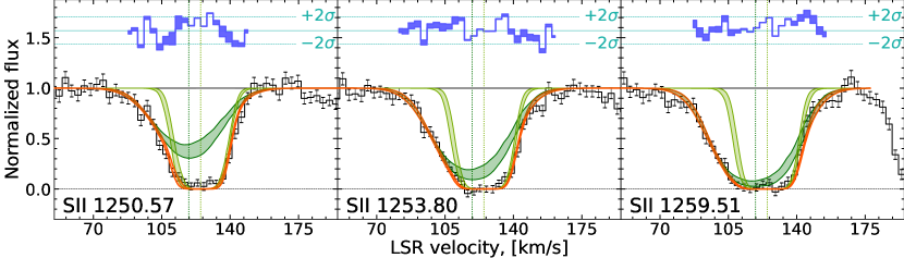
Using HST spectra we fit C i absorption lines from three fine-structure levels (denoted below as C i, C i and C i∗∗) with an assumption of tied redshifts and Doppler parameters between them. This is reasonable approximation, since C i levels are mostly populated by collisions and hence typically quite homogeneously populated within the cloud, unless density and temperatures do not drastically change. Since we study C i in highly saturated H2 clouds, where molecular hydrogen is already self-shielded, the temperature variations are likely small.

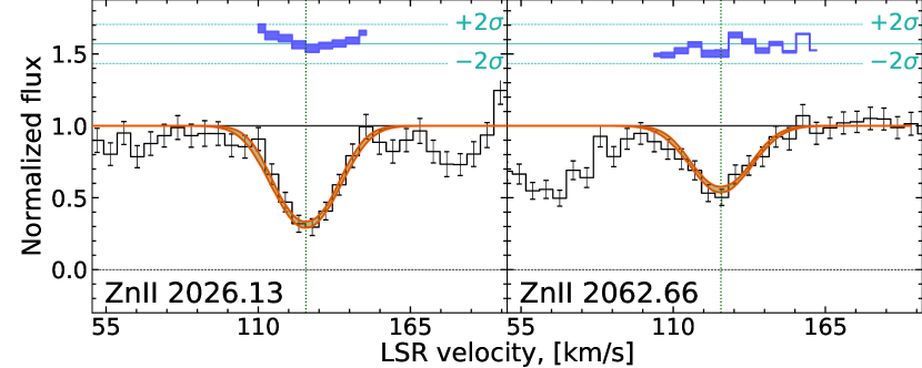
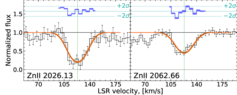
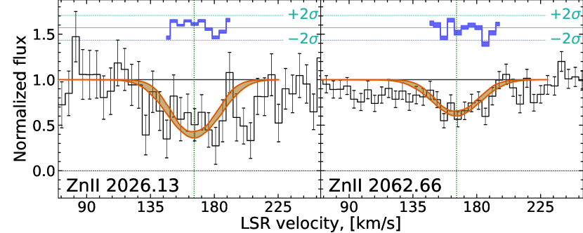
An important ingredient for determination of the physical conditions in the gas phase is metallicity. We measure metallicity in the systems using Zn ii or (if possible) P ii absorption lines, which are believed to be weakly depleted (De Cia et al., 2018). In other cases we use S ii absorption lines. The column density of H i was taken from Welty et al. 2012; Roman-Duval et al. 2019. The metallicity was calculated as, $Z\equiv[{\rm X/H}]\equiv\log\left(N({\rm X})/N({\rm H})\right)-\log\left({\rm X/H}\right)_{\odot}$, where X - is an element used to derive metallicity, and solar abundances, $\left({\rm X/H}\right)_{\odot}$ are taken from Asplund et al. 2009.

3.2 Details on some individual sightlines

Below we provide some details regarding several interesting sightlines.

3.2.1 Sk-67 5

The star is located in diffuse H ii region on the Western edge of the LMC. Tchernyshyov et al. 2015; Roman-Duval et al. 2021 exhaustively studied metals in this system, using HST data, and our measurement of Zn ii column density ($12.98^{+0.02}_{-0.01}$) is consistent with their results ($13.03\pm 0.02$). Additionally, Roman-Duval et al. 2019, 2021 studied H i and C i (for H i they got $21.02\pm 0.04$, which agrees well with value found by Welty et al. 2012, therefore we used a value given by Welty et al. 2012). We got total $\log N(\mbox{C\,{\sc i}})$ to be $14.02^{+0.02}_{-0.01}$ (we fitted with 3 components in the LMC), slightly higher than obtained by Roman-Duval et al. 2021, $13.86^{+0.01}_{-0.01}$ (a similar value was also obtained by Welty et al. 2016). Meanwhile our relative abundance on C i levels are well consistent with obtained by Roman-Duval et al. 2021, while their column densities $\log N(\mbox{C\,{\sc i}})=13.65\pm 0.02$, $\log N(\mbox{C\,{\sc i}}^{*})=13.32\pm 0.02$, $\log N(\mbox{C\,{\sc i}}^{**})=12.86^{+0.04}_{-0.05}$ resemble what we derived in the central component of C i profile.

3.2.2 Sk-67 105

Sk-67 105 is one of the most massive eclipsing binary system (Niemela & Morrell, 1986) in the LMC, which probably reveals a contact configuration with 48.3$M_{\odot}$ and 31.4$M_{\odot}$ (Ostrov & Lapasset, 2003). From H2 lines (mostly from saturated $\rm J=0$ and 1) we found an evidence of partial coverage of absorption system towards Sk-67 105. To get more reliable results we corrected fit of H2 lines for partial covering factor found to be $0.888^{+0.002}_{-0.002}$.

Also we used HST archival data to measure C i fine-structure level population in this system and found that our results are consistent with the values obtained by Roman-Duval et al. 2021. Our result on Zn ii column density $\log N(\rm ZnII)=12.87^{+0.05}_{-0.08}$ is also consistent with the result of Roman-Duval et al. 2021 and therefore gives one of the lowest metallicity in our LMC sample.

3.2.3 Sk-68 135

The star is located in the north of 30 Dor complex, one of the most studied star-forming regions. Metals and C i have been studied by Tchernyshyov et al. 2015; Roman-Duval et al. 2021. Roman-Duval et al. 2021 found $\log N(\mbox{C\,{\sc i}})=14.17^{+0.04}_{-0.05}$, $\log N(\mbox{C\,{\sc i}}^{*})=13.97\pm 0.03$, $\log N(\mbox{C\,{\sc i}}^{**})=13.55\pm 0.04$ which agrees with our results, except C i, which we found to be slightly larger. Our result on Zn ii column density $13.35\pm 0.01$ agrees with a value $13.36\pm 0.06$ found by Tchernyshyov et al. 2015.

3.2.4 Sk-69 246

This star belongs to 30 Dor complex and the system on the line-of-sight have previously been studied by Bluhm & de Boer 2001 and André et al. 2004. These authors reported CO molecules in this system, using FUSE spectra, however, we checked that HST data and do not confirm the detection of CO at reported column density.

Our results on C i, C i and C i∗∗ column densities are close to that of André et al. 2004. They used FUSE spectra, where almost all lines are blended, and HST/STIS (only lines near 1275 Å), while we additionally used the strongest 1656, 1560 and 1328 Å lines. Also we found an excellent agreement with results on C i provided by Roman-Duval et al. 2021. Zn ii column density measured by us ($\log N(\mbox{Zn\,{\sc ii}})=13.32^{+0.01}_{-0.02}$) is a bit lower then $13.38\pm 0.04$ found by Roman-Duval et al. 2021.

3.2.5 AV 95

The star AV 95 belongs to the bar of SMC and the system towards AV 95 have previously been studied by André et al. 2004; Tchernyshyov et al. 2015; Jenkins & Wallerstein 2017. For C i, C i and C i∗∗ we could place only upper limits on column densities due to low S/N of the spectrum and weakness of the lines. André et al. 2004 reported measurements, but, as was noted above, they used only lines seen in the FUSE spectra and lines around 1275 Å  from HST/STIS data, while we additionally used stronger carbon lines in HST high-resolution spectrum. Our estimate on Zn ii column density, $\log N(\mbox{ZnII})=13.08\pm 0.02$, agrees with both values $13.09^{+0.05}_{-0.06}$ and $13.15\pm 0.03$ found by Tchernyshyov et al. 2015 and Jenkins & Wallerstein 2017, respectively.

3.2.6 AV 242

In the system towards AV 242 we found an evidence of high velocity clouds (HVC), which contains H2 molecules (see Paper I). To our knowledge, it is the first found HVC towards the SMC containing H2 and it had not been discussed before. We also found C i  in this HVC $\log N_{\rm HVC}(\rm CI)=12.91^{+0.05}_{-0.08}$ and $\log N(\rm ZnII)=12.66^{+0.09}_{-0.10}$. Metal lines have been studied by Jenkins & Wallerstein 2017, their reported Zn ii  column density, $13.39^{+0.14}_{-0.21}$, is consistent with ours measured value $13.17^{+0.04}_{-0.05}$ summed over the components. However, as Jenkins & Wallerstein 2017 used AOD method, they could not separate subcomponents seen in this sightline.

3.2.7 Sk 191

We found one of the highest H2 column density along the sightline towards Sk 191, while there was lack of Zn ii in this system. On the one hand, this can be explained by exceptionally low metallicity. The star is located close to Magellanic Bridge, which reveals abundances lower than in the LMC and SMC, therefore the medium in front of Sk 191 may have lower metallicity. But on the other hand, the environment may have an especially high depletion and a possible detection of O i by Jenkins & Wallerstein 2017 confirms this assumption. Also such a high H2 column density may possibly be an evidence of high depletion, since H2 forms mainly on the surface of dust grains and correlates with amount of dust (Telikova et al., 2022).

4 Results

C i absorption was detected towards the majority of the studied sightlines (22 out of 28 systems in the SMC and 29 out 29 systems in the LMC). The excitation of C i fine-structure levels was measured in 23 systems in the LMC and 12 systems in the SMC. The fitting results are summarized in Tables 1 and 2 for the LMC and SMC, respectively. Fit to the line profiles are shown in the Appendix A.

Table 1: The fit results of C i towards the LMC sight lines.
Star $v_{\rm LSR}$ $b$, km/s $\log N(\mbox{C\,{\sc i}})$ $\log N(\mbox{C\,{\sc i}}^{*})$ $\log N(\mbox{C\,{\sc i}}^{**})$
Sk-67 2 $266.9(^{+0.2}_{-0.1})$ $3.7^{+0.4}_{-0.4}$ $13.60^{+0.02}_{-0.02}$ $13.43^{+0.03}_{-0.02}$ $13.04^{+0.04}_{-0.04}$
$276.3(^{+0.1}_{-0.2})$ $1.5^{+0.1}_{-0.1}$ $14.02^{+0.07}_{-0.08}$ $13.88^{+0.05}_{-0.03}$ $13.43^{+0.04}_{-0.03}$
Sk-67 5 $279.8^{+0.4}_{-0.6}$ $5.7^{+1.5}_{-0.9}$ $12.96^{+0.05}_{-0.06}$ $12.64^{+0.07}_{-0.13}$ $12.17^{+0.22}_{-0.34}$
$287.35^{+0.05}_{-0.05}$ $1.2^{+0.1}_{-0.1}$ $13.64^{+0.03}_{-0.04}$ $13.29^{+0.02}_{-0.03}$ $12.71^{+0.04}_{-0.06}$
$293.795^{+0.002}_{-0.025}$ $1.9^{+0.3}_{-0.1}$ $13.09^{+0.02}_{-0.03}$ $12.84^{+0.04}_{-0.04}$ $12.24^{+0.11}_{-0.13}$
Sk-67 20 $286.03^{+0.08}_{-0.11}$ $4.2^{+0.2}_{-0.2}$ $13.46^{+0.01}_{-0.02}$ $13.44^{+0.01}_{-0.01}$ $12.97^{+0.03}_{-0.02}$
PGMW 3070 $284.1^{+0.2}_{-0.2}$ $4.4^{+0.5}_{-0.3}$ $13.34^{+0.03}_{-0.02}$ $13.18^{+0.03}_{-0.03}$ $12.73^{+0.10}_{-0.09}$
LH 10-3120 $263.9^{+0.2}_{-0.4}$ $1.0^{+0.5}_{-0.4}$ $12.98^{+0.15}_{-0.08}$ $12.93^{+0.06}_{-0.08}$ $\lesssim 13.1$
$281.3^{+0.4}_{-0.4}$ $7.8^{+0.7}_{-0.6}$ $13.32^{+0.02}_{-0.03}$ $13.06^{+0.04}_{-0.06}$ $12.77^{+0.09}_{-0.08}$
PGMW 3223 $269.5^{+0.3}_{-0.6}$ $6.4^{+1.0}_{-0.6}$ $13.43^{+0.03}_{-0.05}$ $13.35^{+0.04}_{-0.05}$ $13.05^{+0.06}_{-0.07}$
$287.2^{+0.9}_{-1.2}$ $4.0^{+3.5}_{-3.5}$ $12.75^{+0.19}_{-0.13}$ $12.75^{+0.18}_{-0.23}$ $12.68^{+0.13}_{-0.13}$
Sk-66 35 $271.3^{+0.4}_{-0.4}$ $7.6^{+1.0}_{-0.6}$ $13.35^{+0.03}_{-0.03}$ $13.15^{+0.04}_{-0.04}$ $12.64^{+0.10}_{-0.16}$
Sk-66 51 $302.6^{+18.2}_{-167.3}$ $7.0^{+13.0}_{-6.5}$ $12.9^{+0.4}_{-1.0}$ $\lesssim 13.5$ $\lesssim 14.4$
$307.6^{+1.2}_{-0.7}$ $0.7^{+4.8}_{-0.2}$ $13.14^{+0.09}_{-0.11}$ $13.07^{+0.08}_{-0.10}$ $\lesssim 12.6$
Sk-70 79 $232.2^{+0.1}_{-0.1}$ $5.9^{+0.1}_{-0.1}$ $13.77^{+0.01}_{-0.01}$ $13.98^{+0.01}_{-0.01}$ $13.71^{+0.01}_{-0.01}$
Sk-68 52 $242.2^{+0.1}_{-0.1}$ $1.8^{+0.3}_{-0.3}$ $13.36^{+0.09}_{-0.08}$ $13.66^{+0.05}_{-0.05}$ $13.34^{+0.06}_{-0.04}$
Sk-71 8 $215.5^{+0.6}_{-0.8}$ $6.8^{+1.3}_{-1.0}$ $13.06^{+0.07}_{-0.08}$ $13.37^{+0.05}_{-0.05}$ $13.23^{+0.05}_{-0.06}$
$229.9^{+1.5}_{-1.5}$ $4.4^{+2.8}_{-2.0}$ $12.74^{+0.16}_{-0.15}$ $12.60^{+0.27}_{-0.27}$ $12.58^{+0.22}_{-0.29}$
Sk-69 106 $249.7^{+0.1}_{-0.1}$ $5.1^{+0.3}_{-0.2}$ $13.30^{+0.02}_{-0.02}$ $13.57^{+0.01}_{-0.01}$ $13.44^{+0.01}_{-0.02}$
Sk-68 73 $292.7^{+0.3}_{-0.4}$ $8.7^{+0.5}_{-0.5}$ $13.71^{+0.03}_{-0.04}$ $13.84^{+0.03}_{-0.06}$ $13.59^{+0.05}_{-0.05}$
$295.4^{+0.1}_{-0.1}$ $1.2^{+0.3}_{-0.2}$ $13.76^{+0.13}_{-0.09}$ $14.08^{+0.16}_{-0.09}$ $13.70^{+0.11}_{-0.11}$
Sk-67 105 $301.9^{+0.1}_{-0.1}$ $1.5^{+0.3}_{-0.2}$ $13.61^{+0.12}_{-0.13}$ $13.73^{+0.06}_{-0.06}$ $13.25^{+0.11}_{-0.05}$
BI 184 $250.4^{+0.4}_{-0.3}$ $1.8^{+0.4}_{-0.3}$ $13.64^{+0.06}_{-0.18}$ $13.44^{+0.04}_{-0.04}$ $13.21^{+0.05}_{-0.07}$
Sk-71 45 $243.7^{+0.6}_{-0.7}$ $12.1^{+1.8}_{-1.2}$ $13.34^{+0.03}_{-0.04}$ $13.37^{+0.05}_{-0.04}$ $13.12^{+0.03}_{-0.07}$
Sk-71 46 $249.7^{+1.2}_{-1.5}$ $10.1^{+0.3}_{-0.3}$ $13.38^{+0.04}_{-0.04}$ $13.42^{+0.04}_{-0.09}$ $13.14^{+0.08}_{-0.03}$
$230.6^{+0.8}_{-2.0}$ $10.0^{+0.1}_{-0.2}$ $13.26^{+0.06}_{-0.04}$ $13.54^{+0.03}_{-0.04}$ $12.75^{+0.13}_{-0.19}$
Sk-69 191 $237.4^{+0.2}_{-0.2}$ $1.0^{+2.0}_{-0.1}$ $12.95^{+0.05}_{-0.04}$ $12.88^{+0.03}_{-0.03}$ $12.32^{+0.11}_{-0.19}$
BI 237 $290.5^{+0.7}_{-0.9}$ $11.6^{+2.5}_{-1.1}$ $13.51^{+0.04}_{-0.03}$ $13.36^{+0.06}_{-0.03}$ $\lesssim 13.2$
Sk-68 129 $278.3^{+0.1}_{-0.3}$ $13.4^{+0.5}_{-0.4}$ $13.72^{+0.01}_{-0.01}$ $13.69^{+0.01}_{-0.01}$ $13.08^{+0.06}_{-0.06}$
Sk-66 172 $282.3^{+0.4}_{-0.3}$ $4.8^{+0.6}_{-0.7}$ $13.13^{+0.04}_{-0.04}$ $13.28^{+0.04}_{-0.03}$ $12.87^{+0.07}_{-0.08}$
$299.6^{+0.3}_{-0.4}$ $5.7^{+0.6}_{-0.7}$ $13.17^{+0.03}_{-0.04}$ $13.39^{+0.04}_{-0.03}$ $12.96^{+0.06}_{-0.05}$
BI 253 $275.0^{+1.0}_{-0.8}$ $14.8^{+0.2}_{-1.3}$ $13.68^{+0.21}_{-0.69}$ $13.4^{+0.3}_{-0.5}$ $13.1^{+0.4}_{-1.0}$
Sk-68 135 $268.0^{+0.2}_{-0.1}$ $0.4^{+0.3}_{-0.2}$ $13.38^{+0.25}_{-0.40}$ $13.44^{+0.17}_{-0.12}$ $12.88^{+0.15}_{-0.14}$
$276.5^{+0.1}_{-0.1}$ $5.8^{+0.3}_{-0.2}$ $14.00^{+0.02}_{-0.02}$ $13.93^{+0.02}_{-0.02}$ $13.45^{+0.02}_{-0.01}$
Sk-69 246 $277.7^{+0.3}_{-0.2}$ $5.0^{+0.4}_{-0.5}$ $13.72^{+0.05}_{-0.07}$ $13.69^{+0.04}_{-0.06}$ $13.33^{+0.02}_{-0.03}$
$286.9^{+0.9}_{-1.8}$ $4.1^{+2.2}_{-1.1}$ $13.25^{+0.16}_{-0.11}$ $13.07^{+0.20}_{-0.15}$ $\lesssim 13.0$
Sk-68 140 $277.7^{+0.1}_{-0.2}$ $8.5^{+0.4}_{-0.4}$ $13.66^{+0.02}_{-0.02}$ $13.78^{+0.01}_{-0.01}$ $13.41^{+0.03}_{-0.02}$
Sk-71 50 $231.2^{+0.6}_{-0.7}$ $5.9^{+1.6}_{-1.0}$ $12.83^{+0.08}_{-0.10}$ $13.19^{+0.05}_{-0.05}$ $12.80^{+0.12}_{-0.11}$
$273.9^{+0.4}_{-0.2}$ $5.6^{+0.6}_{-0.4}$ $13.52^{+0.02}_{-0.04}$ $13.20^{+0.04}_{-0.06}$ $\lesssim 12.7$
Sk-69 279 $276.3^{+0.4}_{-0.3}$ $2.0^{+0.3}_{-0.5}$ $13.83^{+0.52}_{-0.29}$ $13.30^{+0.07}_{-0.05}$ $12.52^{+0.10}_{-0.17}$
Sk-68 155 $289.9^{+0.3}_{-0.3}$ $12.9^{+0.6}_{-0.6}$ $13.67^{+0.02}_{-0.01}$ $13.62^{+0.01}_{-0.02}$ $\lesssim 13.2$
Sk-70 115 $220.72^{+0.03}_{-0.04}$ $2.1^{+0.1}_{-0.1}$ $13.56^{+0.02}_{-0.02}$ $13.52^{+0.01}_{-0.01}$ $13.04^{+0.02}_{-0.02}$
  • Upper limits were constrained from $3\sigma$ confidence interval

Table 2: The fit results of C i towards the SMC sightlines.
Star $v_{\rm LSR}$ $b$, km/s $\log N(\mbox{C\,{\sc i}})$ $\log N(\mbox{C\,{\sc i}}^{*})$ $\log N(\mbox{C\,{\sc i}}^{**})$
AV 6 $128.6^{+1.2}_{-0.9}$ $14.9^{+0.1}_{-1.3}$ $\lesssim 13.02$ $\lesssim 12.89$ $\lesssim 12.84$
AV 15 $132.4^{+0.7}_{-0.6}$ $7.9^{+1.2}_{-1.0}$ $13.20^{+0.05}_{-0.05}$ $13.07^{+0.06}_{-0.08}$ $12.69^{+0.14}_{-0.16}$
AV 26 $122.8^{+0.1}_{-0.1}$ $0.35^{+0.1}_{-0.1}$ $13.78^{+0.06}_{-0.07}$ $13.89^{+0.05}_{-0.06}$ $13.53^{+0.04}_{-0.04}$
$125.02^{+0.05}_{-0.07}$ $0.22^{+0.1}_{-0.1}$ $15.16^{+0.06}_{-0.09}$ $14.59^{+0.11}_{-0.09}$ $13.82^{+0.10}_{-0.07}$
AV 47 $121.7^{+1.5}_{-1.5}$ $13.4^{+1.7}_{-2.2}$ $12.83^{+0.09}_{-0.11}$ $13.00^{+0.06}_{-0.09}$ $\lesssim 12.8$
AV 69 $127.7^{+0.9}_{-1.4}$ $7.4^{+2.6}_{-6.9}$ $12.81^{+0.08}_{-0.09}$ $12.77^{+0.11}_{-0.10}$ $\lesssim 12.5$
AV 75 $117.8^{+0.9}_{-0.9}$ $6.2^{+1.2}_{-1.1}$ $12.95^{+0.09}_{-0.07}$ $13.02^{+0.17}_{-0.18}$ $13.06^{+0.09}_{-0.07}$
AV 80 $116.3^{+0.2}_{-0.5}$ $8.9^{+0.9}_{-0.8}$ $13.35^{+0.04}_{-0.03}$ $13.16^{+0.04}_{-0.06}$ $12.63^{+0.11}_{-0.24}$
AV 81 $149.6^{+0.9}_{-1.2}$ $6.3^{+2.3}_{-1.7}$ $13.06^{+0.07}_{-0.10}$ $12.63^{+0.27}_{-0.52}$ $\lesssim 12.8$
AV 95 $122.3^{+0.9}_{-1.5}$ $5.2^{+2.7}_{-1.1}$ $\lesssim 13.0$ $\lesssim 12.8$ $\lesssim 12.9$
AV 104 $116.6^{+2.4}_{-0.9}$ $<8$ $\lesssim 14.56$ $\lesssim 13.72$ $\lesssim 13.82$
AV 170 $128.6^{+0.3}_{-0.5}$ $0.5^{+0.1}_{-0.1}$ $13.56^{+0.32}_{-0.26}$ $\lesssim 13.4$ $\lesssim 13.2$
AV 175 $136.4^{+1.8}_{-1.5}$ $22.3^{+2.9}_{-2.5}$ $13.20^{+0.05}_{-0.09}$ $\lesssim 13.4$ $\lesssim 13.4$
AV 207 $164.0^{+1.0}_{-0.7}$ $1.2^{+4.4}_{-0.8}$ $12.99^{+0.25}_{-0.17}$ $13.25^{+0.12}_{-0.13}$ $\lesssim 14.5$
AV 210 $162.8^{+0.9}_{-0.6}$ $5.4^{+1.5}_{-1.6}$ $13.07^{+0.07}_{-0.07}$ $13.07^{+0.08}_{-0.09}$ $\lesssim 13.0$
AV 215 $127.0^{+0.9}_{-0.8}$ $6.4^{+1.4}_{-1.5}$ $13.35^{+0.06}_{-0.08}$ $12.74^{+0.26}_{-0.45}$ $\lesssim 12.8$
$142.7^{+1.5}_{-1.8}$ $7.8^{+4.7}_{-1.0}$ $13.16^{+0.12}_{-0.12}$ $13.03^{+0.17}_{-0.06}$ $12.66^{+0.27}_{-0.17}$
AV 216 $142.9^{+0.4}_{-0.5}$ $2.3^{+1.0}_{-0.8}$ $12.88^{+0.06}_{-0.07}$ $12.76^{+0.08}_{-0.12}$ $12.49^{+0.17}_{-0.19}$
AV 243 $128.9^{+1.5}_{-1.2}$ $1.0^{+1.1}_{-0.9}$ $\lesssim 15.7$ $\lesssim 13.7$ $\lesssim 14.7$
AV 242 $92.9^{+0.6}_{-0.7}$ $3.6^{+1.0}_{-1.5}$ $12.70^{+0.06}_{-0.07}$ $\lesssim 12.7$ $\lesssim 12.4$
$158.4^{+0.4}_{-0.8}$ $4.1^{+1.4}_{-1.9}$ $12.86^{+0.13}_{-0.12}$ $\lesssim 12.8$ $\lesssim 12.4$
AV 266 $127.6^{+0.7}_{-0.6}$ $6.8^{+1.4}_{-0.9}$ $13.11^{+0.04}_{-0.04}$ $12.73^{+0.11}_{-0.09}$ $\lesssim 12.6$
AV 372 $143.2^{+0.3}_{-0.2}$ $5.7^{+0.5}_{-0.5}$ $13.40^{+0.02}_{-0.03}$ $12.95^{+0.04}_{-0.08}$ $\lesssim 12.5$
AV 423 $141.2^{+1.8}_{-3.3}$ $9.7^{+0.3}_{-3.5}$ $12.87^{+0.10}_{-0.17}$ $\lesssim 13.1$ $\lesssim 12.6$
$159.2^{+1.5}_{-3.5}$ $9.7^{+0.3}_{-9.2}$ $12.81^{+0.10}_{-0.30}$ $\lesssim 13.1$ $\lesssim 12.7$
AV 440 $167.3^{+6.0}_{-7.2}$ $0.5^{+1.6}_{-0.1}$ $\lesssim 15.84$ $\lesssim 13.41$ $\lesssim 16.66$
$116.6^{+2.4}_{-0.9}$ $0.5^{+7.3}_{-0.1}$ $\lesssim 16.87$ $\lesssim 15.40$ $\lesssim 17.29$
AV 472 $126.8^{+1.8}_{-1.8}$ $0.7^{+0.2}_{-0.2}$ $\lesssim 15.7$ $\lesssim 13.8$ $\lesssim 16.6$
AV 476 $159.2^{+1.5}_{-1.8}$ $12.9^{+1.3}_{-1.8}$ $13.15^{+0.10}_{-0.07}$ $13.07^{+0.05}_{-0.09}$ $13.03^{+0.07}_{-0.10}$
$168.7^{+0.3}_{-0.1}$ $1.0^{+0.2}_{-0.2}$ $15.40^{+0.50}_{-0.60}$ $14.39^{+0.29}_{-0.30}$ $13.97^{+0.25}_{-0.12}$
AV 479 $158.5^{+0.1}_{-0.2}$ $1.9^{+0.3}_{-0.3}$ $12.71^{+0.04}_{-0.03}$ $12.61^{+0.05}_{-0.06}$ $12.07^{+0.10}_{-0.18}$
$164.1^{+0.2}_{-0.4}$ $1.4^{+0.8}_{-0.5}$ $12.24^{+0.10}_{-0.11}$ $12.36^{+0.08}_{-0.09}$ $\lesssim 12.2$
AV 488 $143.2^{+0.4}_{-0.5}$ $5.9^{+0.8}_{-0.9}$ $13.08^{+0.04}_{-0.04}$ $12.59^{+0.11}_{-0.14}$ $\lesssim 12.5$
AV 490 $133.5^{+0.1}_{-0.1}$ $4.9^{+0.2}_{-0.1}$ $13.50^{+0.01}_{-0.01}$ $12.94^{+0.02}_{-0.02}$ $12.15^{+0.09}_{-0.07}$
Sk 191 $134.6^{+1.5}_{-1.8}$ $9.2^{+3.8}_{-3.4}$ $12.88^{+0.09}_{-0.12}$ $\lesssim 13.10$ $\lesssim 12.74$
$153.7^{+0.4}_{-0.3}$ $4.5^{+1.0}_{-0.7}$ $13.34^{+0.03}_{-0.05}$ $13.42^{+0.03}_{-0.06}$ $13.05^{+0.07}_{-0.05}$
  • Upper limits were constrained from $3\sigma$ confidence interval

4.1 Metallicity

The measurements of metallicity are given in the second column of Tables 3 and 4 for the LMC and SMC, respectively and lines are shown in the Appendix B. The average metallicity in our sample is $\log Z_{\rm LMC}\sim-0.66$ with dispersion of 0.22 and $\log Z_{\rm SMC}\sim-0.99$ with standard deviation of 0.19 for the LMC and SMC, respectively. It is less by $-0.3$ dex and $-0.7$ dex than the average gas phase metallicity measured in local MW ISM (e.g., Ritchey et al., 2023). These values are consistent with previous values reported in literature ($\log Z^{*}\sim-0.2$ for the LMC and $\log Z^{*}\sim-0.6$ for the SMC relative to local ISM, Russell & Dopita 1992). The difference in absolute values are partially due to the difference in solar abundances between Anders & Grevesse (1989) and Asplund et al. (2009). Also it can be explained by depletion of metals by dust and usage of the different species, or selection effects, since our targets probe a cold phase of the ISM. Meanwhile, even in local ISM the value of metallicity is debatable and possibly has large variations De Cia et al. 2021, but see also Ritchey et al. (2023).

4.2 C i/H2 abundances

Refer to caption
Refer to caption
Figure 1: Left panel: H2 and C i column densities. The blue squares, red diamonds, yellow triangles and green circles show the measurements in SMC, LMC, Milky Way (Rachford et al., 2002, 2009; Burgh et al., 2010; Jenkins & Tripp, 2011; Shull et al., 2021; Ritchey et al., 2023) and high redshift DLAs (Noterdaeme et al., 2018; Balashev et al., 2019; Srianand et al., 2005; Ledoux et al., 2003; Jorgenson et al., 2009, 2010), respectively. Dashed lines show C i/H2 ratios equal to -4, -5, -6, -7. Right panel: $\log N({\rm CI})/N({\rm H_{2}})$ as a function of gas-phase metallicity. The symbols are the same as in left panel.

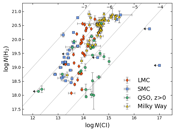
In the left panel of Fig. 1 we show the column densities of C i and H2 in the LMC and SMC and their comparison with measurements in the Milky Way (Jenkins & Tripp, 2011) and in high redshift DLAs (see, e.g. Klimenko & Balashev, 2020, and references therein). We found that on average C i column densities in the SMC is less than in the LMC and both are less than in the MW and DLAs. The difference in C i abundance (and C i/H2 relative abundance) between the LMC, SMC and MW can be due to the difference in gas phase metallicity. A higher C i abundances in high-z DLAs can be due to the selection effect (many C i bearing high-z DLAs were preselected by the presence of strong C i in SDSS spectra, see e.g. Noterdaeme et al. 2018) and/or distinct physical conditions. Both these factors likely explain large dispersion of C i/H2 ratios measured at high-z.

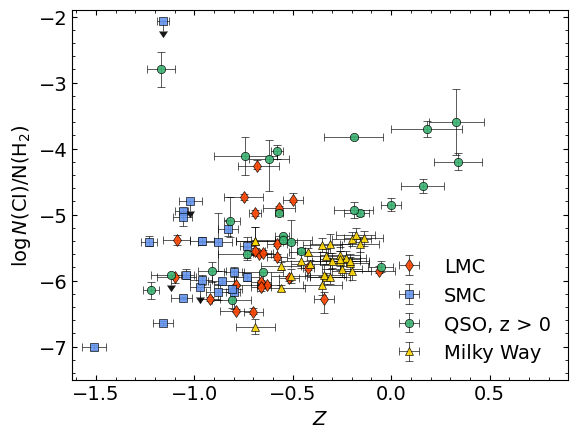
The right panel of Fig 1 shows C i/H2 relative abundance as a function of metallicity in different samples. While the C i abundance is evidently scaled with the total carbon abundance in the medium, and hence metallicity333The system towards Q 0347-3819 (Srianand et al., 2005) has an exceptionally high C i/H2 ratio among low metallicity systems due to low H2 abundance., it also strongly depends on the chemistry of the clouds, since C i is not the dominant form of the carbon in diffuse clouds. Indeed the formation rate of C i depends on the metallicity, since it is produced from C ii either by recombination with electron or small dust grains (Wolfire et al., 2008). Both electron and dust abundances, interactively depend on the metallicity, especially at the low values of the latter. Moreover H2 abundance scales with the metallicity as well, since the main formation channel of H2 molecules is the formation on the surface of dust grains, which abundance is proportional with the metallicity. Therefore dependence of C i/H2 ratio on the metallicity is relatively complicated and requires comprehensive modelling. We will exhaustively consider C i/H2 abundance in a separate study (Balashev&Kosenko in prep.).

4.3 Kinetic temperature

Refer to caption
Figure 2: H2 excitation temperature as a function of H2 column density. The symbols are the same as in Fig. 1, except yellow triangles show Milky Way values from Savage et al. 1977; Gillmon et al. 2006 (see discussion in Sect. 4.3).
Refer to caption
Figure 3: $f_{1}^{\prime}=N(\mbox{C\,{\sc i}}^{*})/N(\mbox{C\,{\sc i}})$ vs $f_{2}^{\prime}=N(\mbox{C\,{\sc i}}^{**})/N(\mbox{C\,{\sc i}})$. Here red diamonds are measurements in the LMC, blue squares are measurements in the SMC, green circles are QSO data (from the references provided in caption of Fig. 1) and yellow triangles are data in the MW (Jenkins & Tripp, 2011). Model curves are calculated for the temperatures $T=50$, 100 and 200  K, and number densities in the range $\log n=0-5$ assuming only atomic hydrogen ($f_{\rm H_{2}}=0$, solid curves) and full molecularized case ($f_{\rm H_{2}}=1$, dashed curves).

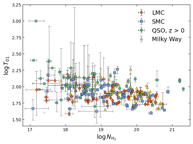
It is well known that bulk of H2 J=0 and J=1 reside in the inner, self-shielded part of the medium (see e.g. Balashev et al., 2009; Klimenko & Balashev, 2020) reflecting its thermal state. As it was done previously in many studies, we used H2 ortho-para (determined by J=0, 1) excitation temperature, $T_{01}$ to constrain the kinetic temperature of cold phase of ISM, probed by H2/C i absorptions. Fig. 2 shows H2 excitation temperature as a function of H2 column density, measured in Magellanic Clouds (taken from paper I), in our Galaxy (Savage et al., 1977; Gillmon et al., 2006), and at high-redshifts (see e.g. Balashev et al., 2019, and references therein). One can see that Magellanic Cloud sample, consistent with both high-redshift and MW sample over most of the range of $N_{\rm H_{2}}$ column density. However, we note that recently an extensive survey of H2 in our Galaxy based on FUSE data by Shull et al. 2021 reveals higher $T_{01}$ temperatures, that were previously derived by Savage et al. 1977; Gillmon et al. 2006; Rachford et al. 2002, 2009. This discrepancy if it is real, devotes an additional study. Apart from this, we definitely see that our measurements confirm the trend of decreasing $T_{01}$ with increase of H2 column density for the Magellanic Cloud sample (previously reported for the MW and high-z samples by Muzahid et al., 2015; Balashev et al., 2017; Klimenko & Balashev, 2020). However, due to large scatter, the correlation for Magellanic Clouds is weak, but significant (Pearson correlation coefficients are about $-0.16$ and -0.14 with p-values $5.3\times 10^{-5}$ and $3.7\times 10^{-5}$ for LMC and SMC, respectively). We find a similar correlation for the sample of high-redshift DLAs ($r=-0.14$ with $p$-value of 0.0006), which cover the same range of H2 column densities. The correlation in the MW sample (using temperatures reported by Savage et al. 1977; Gillmon et al. 2006 data) is stronger: $r=-0.49$ with $p$-value $1.4\times 10^{-7}$. However the MW sample probe more saturated H2 gas clouds, than other samples.

4.4 Excitation of fine structure levels

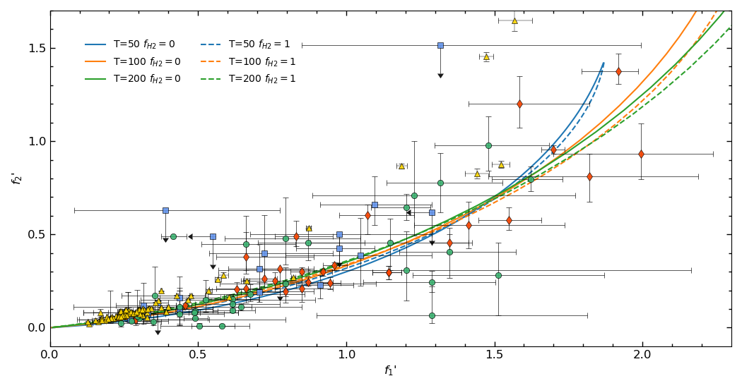
In the Fig. 3 we plot C i column density ratios $f_{1}^{\prime}=N(\mbox{C\,{\sc i}}^{*})/N(\mbox{C\,{\sc i}})$ vs $f_{2}^{\prime}=N(\mbox{C\,{\sc i}}^{**})/N(\mbox{C\,{\sc i}})$444Note that Jenkins & Tripp 2001, 2011 used $f_{1}=N(\mbox{C\,{\sc i}}^{*})/N(\mbox{C\,{\sc i}}_{\rm tot})$ and $f_{2}=N(\mbox{C\,{\sc i}}^{**})/N(\mbox{C\,{\sc i}}_{\rm tot})$ in their works. However, the plots $f_{1}$-$f_{2}$ and $f_{1}^{\prime}$-$f_{2}^{\prime}$ look quite similar.. measured in Magellanic Clouds, Milky Way and high-redshift galaxies. One can see that measurements at high redshifts show large dispersion, as Magellanic Clouds values, while measurements in our Galaxy reveal systematically lower excitation of the upper fine-structure levels. The possible explanation is lower UV field intensity in Milky Way (as the main sources of C i  excitation are collisions and excitation by UV radiation and CMB) and it will be discussed below. We compare these measurements with model curves that were calculated for $T=50,100,200$ K in the range of number densities $n=1-10^{5}\,{\rm cm^{-3}}$. Regarding collisional partner we considered two limiting cases: atomic and molecular hydrogen, denoted it by the molecular fraction parameter, $f_{\rm H_{2}}=2n({\rm H_{2}})/(2n({\rm H_{2}})+n({\rm HI}))$. One can see that measured values follow model tracks, indicating that we likely have no drastic misfits of the line profiles. Importantly, the relatively large uncertainties do not allow to constrain temperature, number density and molecular fraction, using only the measurements on $f_{1}^{\prime}$ and $f_{2}^{\prime}$ ratios, since the parameter space is degenerate. Jenkins & Tripp 2001, 2011 described a method how to constrain number density and fraction of low-pressure gas from C i fine-structure level population, using the additional estimates on the temperature and UV field intensity. To get constraints on $\chi$ their model requires C ii  column densities (using ionization balance for carbon and hydrogen together, see Equations 1 and 2 in Jenkins & Tripp 2011), since carbon is mostly ionized by UV radiation. In our work, we followed a different approach, where the supplemental data was obtained from fit to H2 rotational levels population (see Klimenko & Balashev, 2020). This allows us to get constraints on $n_{\rm H}$ and $\chi$, omitting additional calculations of C ii column density (where we have lack of the direct measurement) and of low and high pressure gas fractions. This is discussed in the next Section.

5 Physical conditions

Number density and UV field strength can be constrained from comparison of the measured populations of H2 rotational and C i fine-structure levels with ones calculated on the grids of models using Meudon PDR code (Klimenko & Balashev, 2020). It was applied systematically to systems at high redshifts (Balashev et al., 2019; Balashev et al., 2020; Klimenko & Balashev, 2020; Kosenko et al., 2021) and also to few systems in the Milky Way, LMC and SMC (Klimenko & Balashev, 2020).

In this work we used only two lower H2 rotational levels ($\rm J\leq 1$), which contains the most of H2 and basically reproduce the thermal balance in the medium since these levels are predominantly populated by collisions and 555Ortho-para ratio of H2 is set by collisions with H+, H, H2, He and H${}^{+}_{3}$ (Le Petit et al., 2006), $J=2$ level in most cases populated by collisions with H and H2 only in the self-shielded part of the H2-bearing medium (see e.g. Balashev et al., 2009). The higher H2 rotational levels ($\rm J\geq 2$) can be significantly populated by UV pumping and therefore may provide a direct measurement of the UV field. However, UV pumping is very sensitive to saturation of H2 resonant lines (as well as the shielding does), and therefore is very sensitive to the exact geometrical model, which is impossible to constrain in observations towards one sightline. In turn, excitation of two lower rotational levels of H2 is sensitive to the thermal balance in the bulk of the medium, which roughly $\propto\chi/n_{\rm H}$ and/or $\zeta/n_{\rm H}$, where $n_{\rm H}$ is a hydrogen gas density, and $\zeta$ is the Cosmic Ray Ionization Rate (CRIR). For high H2 column densities, considered in this study, bulk of the medium represents region of the cloud, where H2 is self-shielded, and hence significantly less biased by the exact geometry of the cloud and anisotropy of the UV field. Additionally, the column density of ground ortho and para levels usually significantly higher than $\rm J\geq 2$ levels, and typically show Lorentzian wings. This makes constraint of the column density less affected by choice of the exact velocity structure of the absorber (which is complicated in FUSE data) and the degeneration with the Doppler parameter. Finally, description of high H2 rotational levels might require dynamical models in contrast to static Meudon PDR models used here. Indeed, $\rm J\geq 2$ can be significantly excited in the outer layers of the cloud (see e.g. Abgrall et al., 1992; Balashev et al., 2009), where H2 is not yet self-shielded, and due to hydrodynamical motions this region can be larger then static models predict, see detailed discussion in Klimenko & Balashev 2020. In general, we found that taking into account H2 ($\rm J\geq 2$) induces systematic increase in derived $\chi$, that requires additional detailed studies.

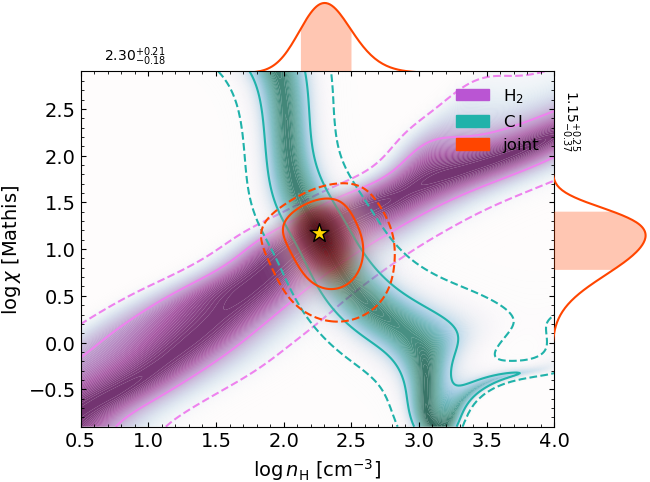
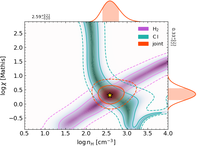
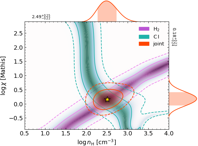
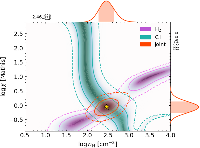
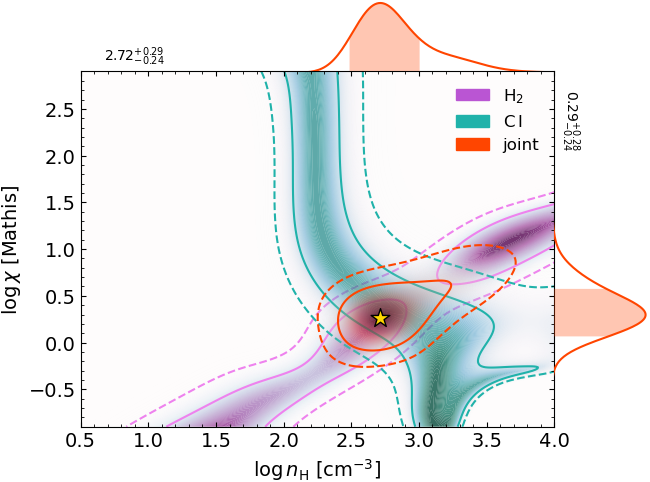
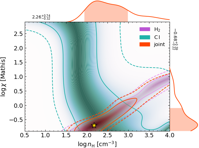
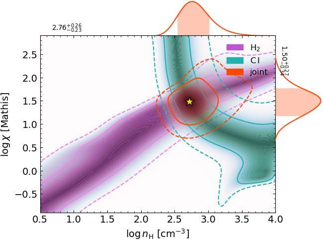
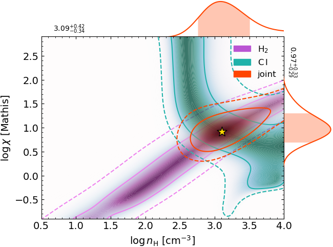
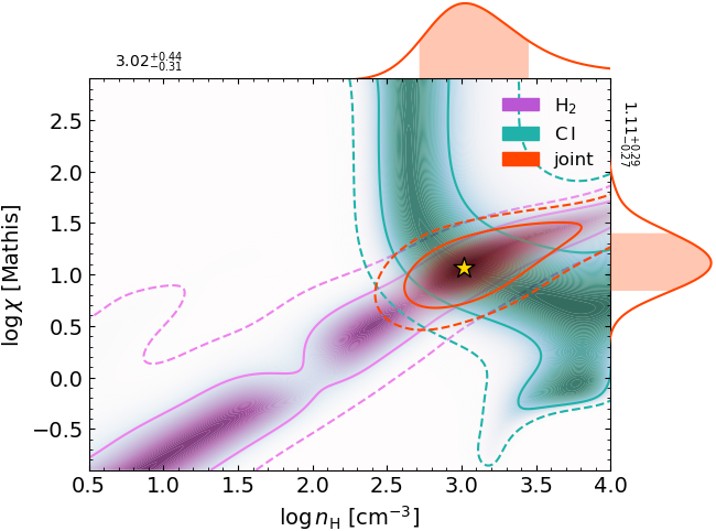
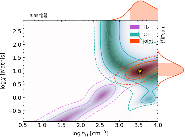
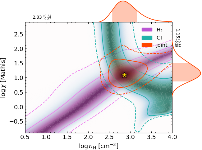
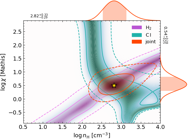
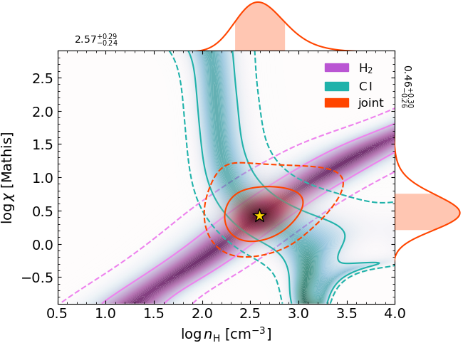
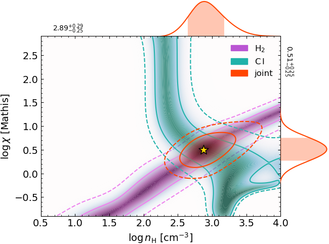
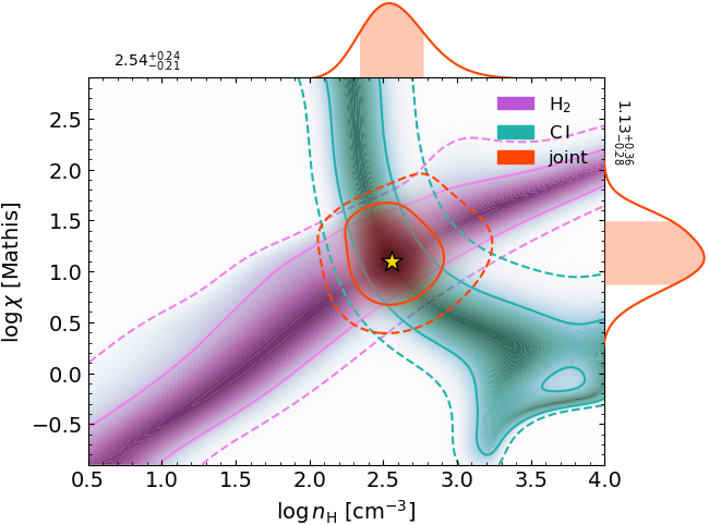
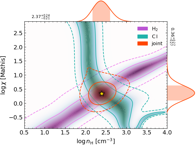
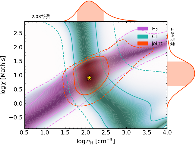
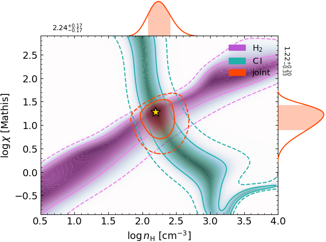
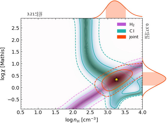
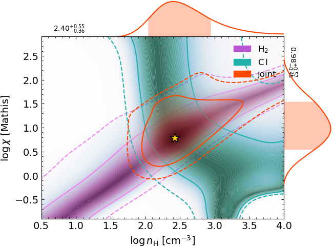
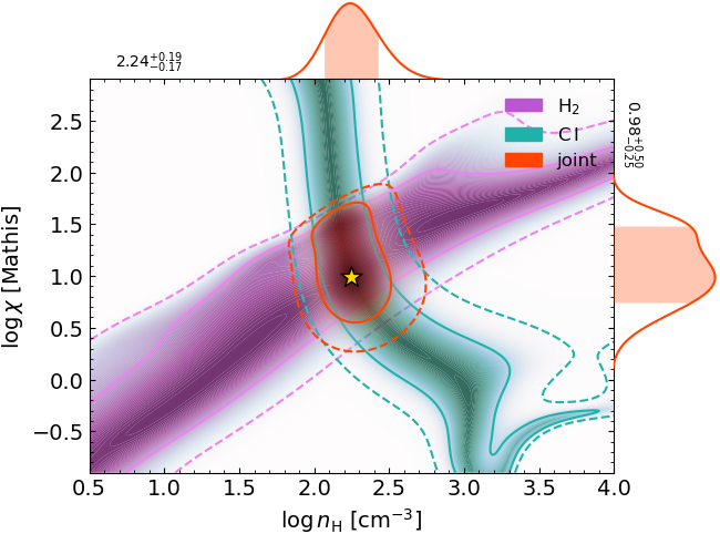
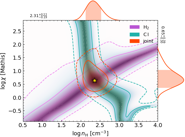
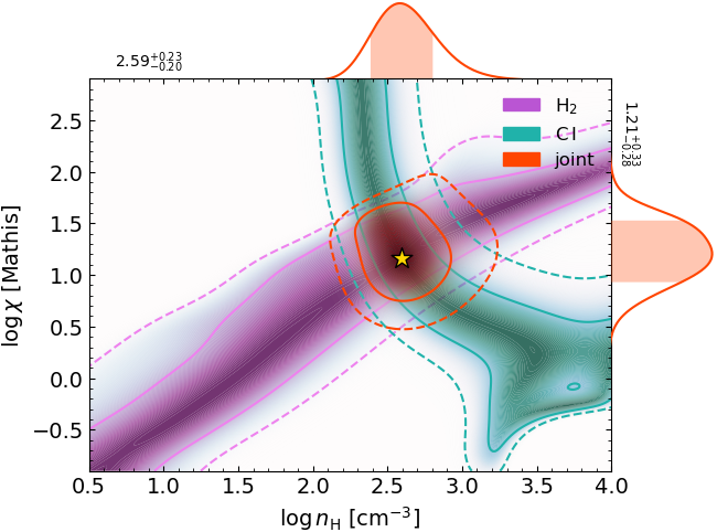
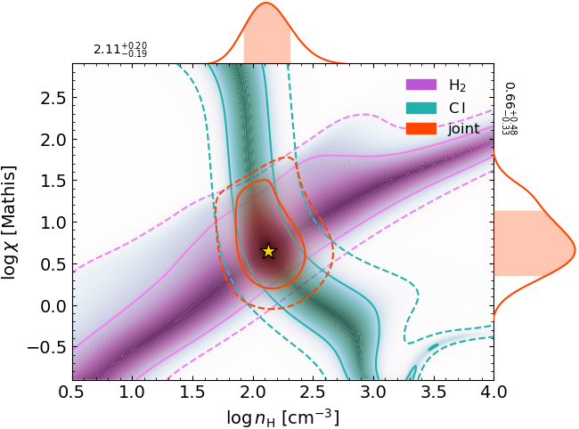
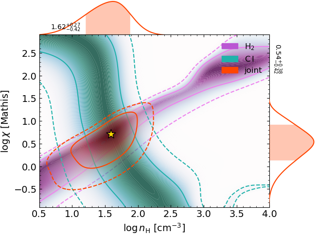
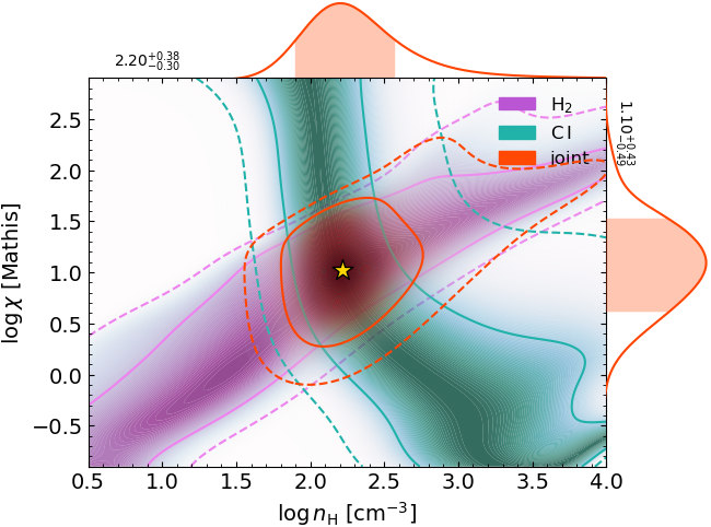
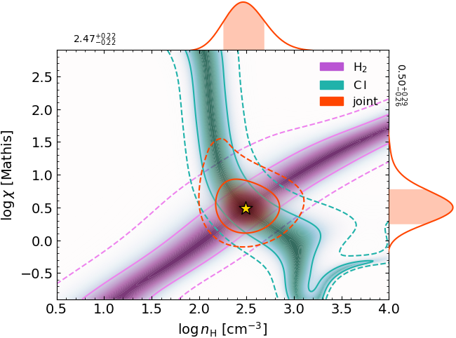
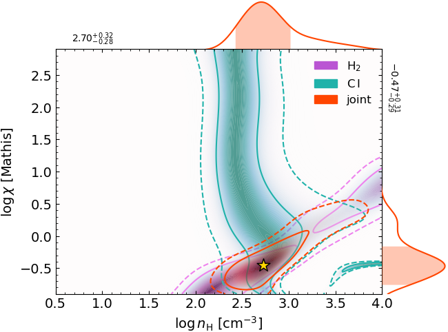
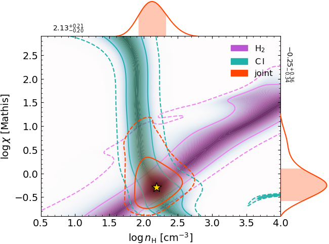
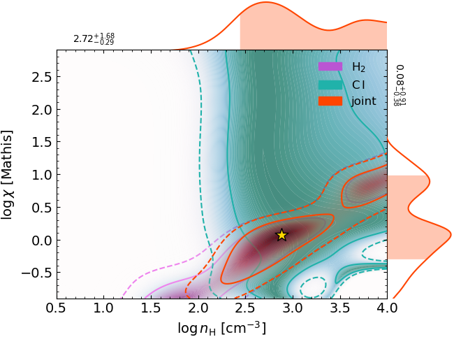
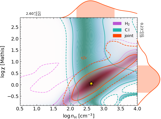
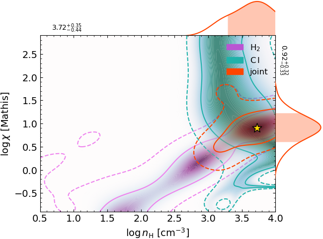
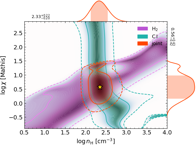
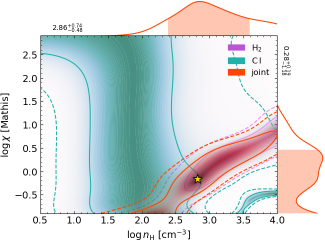
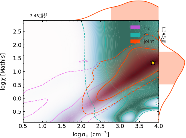
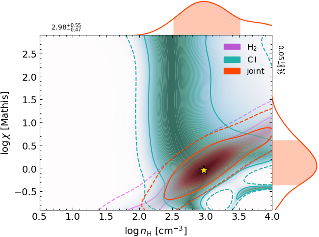
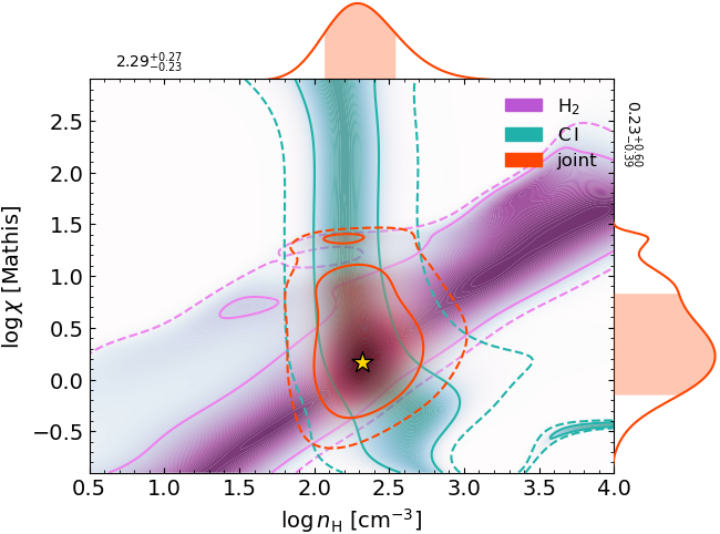
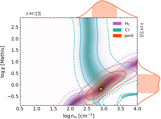
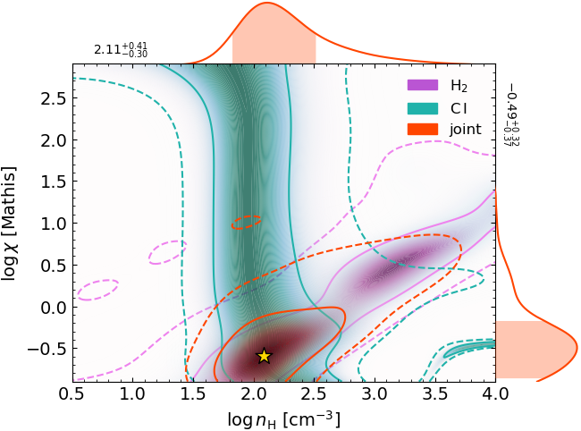
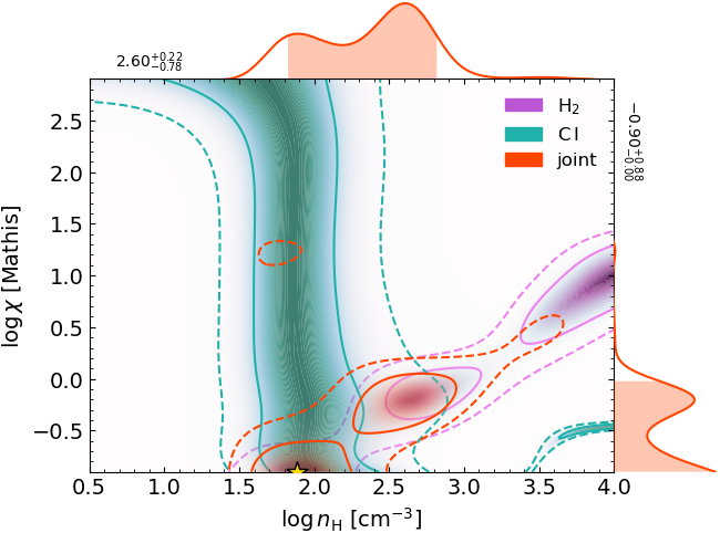
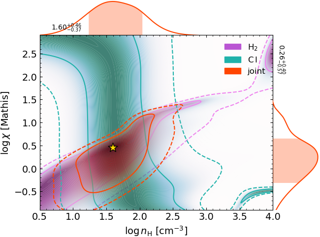
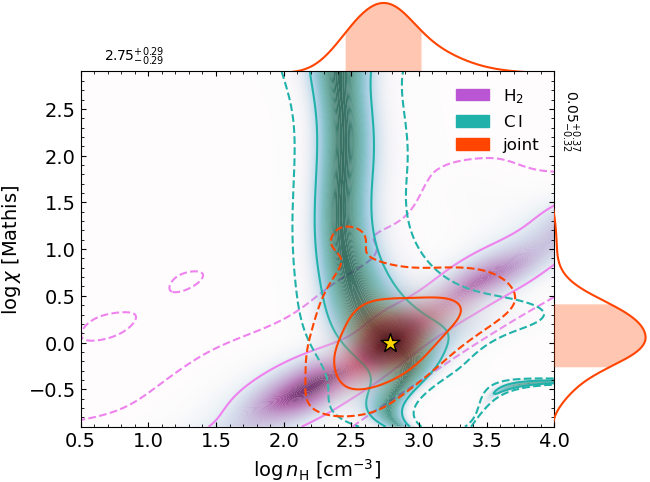
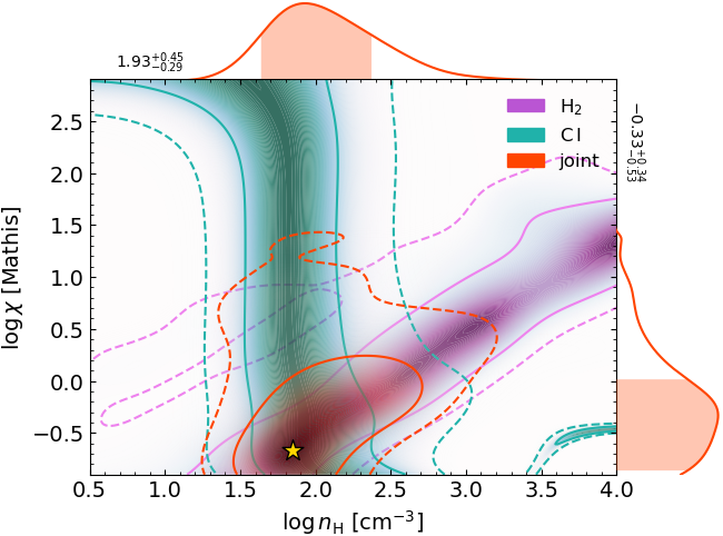
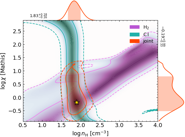
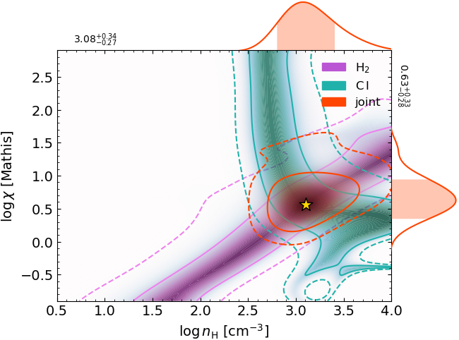
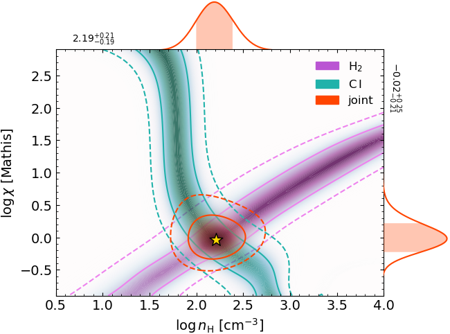
Following Klimenko & Balashev 2020; Kosenko et al. 2021 we obtained a region of $n_{\rm H}$ and $\chi$ values corresponding to fit to the measured column densities of $\rm J=0,1$ levels of H2 levels and C i fine-structure populations. We calculated two grids of constant hydrogen density models with metallicities corresponding to the average metallicities on the LMC and SMC. For each grid we varied $\log n_{\rm H}$ (in units cm-3) and $\log\chi$ (in units of Mathis field (Mathis et al., 1983)) in the ranges [0, 4.5] and [-1, 3], respectively, with the steps 0.5 for both $\log n_{\rm H}$ and $\log\chi$. Note that Meudon PDR used the total hydrogen gas density $n_{\rm H}=n({\rm HI})+2n({\rm H_{2}})$, which close to the gas number density $n_{\rm gas}\approx n({\rm HI})+n({\rm H_{2}})+n(\rm He)$ at low molecular fraction, but can be 2 about times higher for the fully molecular region. We also assumed the CRIR to be linearly scaled with UV field as $\log\zeta_{-16}=\log\chi$, where $\zeta_{-16}$ is a primary ionization rate of the hydrogen atom in the units of $10^{-16}\rm\,s^{-1}$. We made this assumption since Bialy & Sternberg 2019; Balashev et al. 2022 showed that cosmic rays may impact much on the thermal state of the diffuse medium, especially at low metallicity. The linear dependence was taken for simplicity assuming that UV field and cosmic rays are both produced in the star-formation region and likely on average scaled with star-formation rate. For C i we used a relative population of levels, since the ionization state of carbon depends on the chemistry (and hence several physical parameters) and dust properties. In turn, excited C i fine-structure levels, i.e. C i and C i∗∗, are mostly populated by the collisions (which determined by $n_{\rm H}$ and $T$), excitation by the CMB and pumping by UV radiation. However, the latter is typically dominated only at quite high values of UV field (see e.g. Balashev et al., 2019). An example of the constraints on $n_{\rm H}-\chi$ derived from population of C i, low rotational levels of $\rm H_{2}$ and joint analysis is shown in the Fig. 4. One can see that while individual constrains from C i and $\rm H_{2}$ are significantly degenerated, they have different dependence in $n_{\rm H}-\chi(\zeta)$ parameter space, and hence the joint constraint is much tighter than individual ones.

Refer to caption
Figure 4: Estimate on the hydrogen gas density and UV field intensity for the system towards Sk-67 5 in the LMC. The green, violet and red color show the constraints obtained using from C i, H2 and joint analysis. Solid and dashed curves show 0.683 (1$\sigma$) and 0.954 (2$\sigma$) credible intervals for the posterior distribution function, respectively. On the top and left axis we show the marginalized 1d distribution of $n_{\rm H}$ and $\chi$, respectively, where filled regions correspond to 1$\sigma$ estimates, and provide the estimated value in the attached text labels.

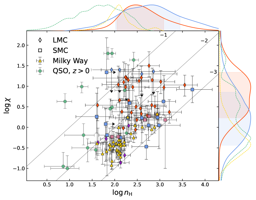
We applied the described method to the systems in the LMC and SMC to get constraints on $n_{\rm H}$ and $\chi(\propto\zeta)$. We used results of H2 fit in spectra obtained with FUSE telescope with resolution $R=\lambda/\Delta\lambda\lesssim 20000$, which is much less then resolution for the most HST data used in this work. Therefore FUSE data does not allow to accurately resolve velocity structure as HST data does and we cannot unambiguously associate H2 and C i  components. Hence we used column densities summarized over all of the Magellanic Clouds components in our analysis. The results are summarize in Tables 3 and 4, and shown in Fig. 5, while the constraints on individual systems are presented in Appendix C. We found that the hydrogen gas densities derived in the LMC and SMC are consistent with the values corresponding to the diffuse cold ISM, $\sim 30-10^{3}\,\rm cm^{-3}$, and with values measured in other H2-bearing absorption systems in the MW and high-$z$ DLAs. The average values of hydrogen gas densities in both the SMC and LMC are close, $\log n_{\rm H}\simeq 2.5$ with dispersion 0.4 for the LMC and $\log n_{\rm H}\simeq 2.6$ and with dispersion 0.6 for the SMC, respectively. Interestingly, that both the SMC and LMC sightlines indicate systematically higher UV field, than ones measured near Solar vicinity, which is in line with previous studies of Magellanic clouds (e.g. Bernard et al., 2008; Sandstrom et al., 2010; Welty et al., 2016; Roman-Duval et al., 2021). The mean value of UV field intensity is $\log\chi\sim 0.3$ with a dispersion 0.5 for the SMC sightlines. This is lower than the mean value in the LMC sightlines $\sim 0.7$ with dispersion 0.4.

Using obtained H2 excitation temperatures and hydrogen densities we found that the thermal pressures666One should bear in mind the above remark about density notation in Meudon PDR  since to get pressures one should use the gas number density, $n_{\rm gas}$. We derived the gas number density as an average over the Meudon model (which assumes constant hydrogen gas density) at particular H2 column density and physical parameters. are on average $\log p/k\simeq 4.2$ and 4.3 with dispersion of about 0.4 and 0.5 for the LMC and SMC, respectively.This is consistent with the values found by Klimenko & Balashev 2020 and by Jenkins & Tripp 2021 for both Magellanic Clouds (their $\log p/k\simeq 4.1\pm 0.5$ and $\simeq 4.0\pm 0.2$, respectively) and Roman-Duval et al. 2021 for the LMC sample (their $\simeq 3.9\pm 0.5$).

Table 3: Physical conditions derived in the absorption systems associated with the LMC
Star $\rm[X/H]$ $\rm X$ $\log n_{\rm H}[\rm cm^{-3}]$ $\log\chi$ $\log\alpha G$
Sk-67 2 $-0.34^{+0.05}_{-0.05}$ Zn $2.30^{+0.21}_{-0.18}$ $1.15^{+0.25}_{-0.37}$ $0.88^{+0.30}_{-0.48}$
Sk-67 5 $-0.58^{+0.05}_{-0.05}$ Zn $2.19^{+0.21}_{-0.19}$ $-0.02^{+0.25}_{-0.21}$ $-0.11^{+0.30}_{-0.32}$
Sk-67 20 $2.59^{+0.22}_{-0.20}$ $0.33^{+0.23}_{-0.21}$ $-0.24^{+0.29}_{-0.33}$
PGMW 3070 $2.49^{+0.25}_{-0.22}$ $0.18^{+0.23}_{-0.24}$ $-0.29^{+0.31}_{-0.38}$
LH10 3120 $-0.75^{+0.10}_{-0.10}$ Zn $2.46^{+0.20}_{-0.19}$ $-0.06^{+0.19}_{-0.0.21}$ $-0.38^{+0.26}_{-0.32}$
PGMW 3223 $-0.57^{+0.08}_{-0.08}$ Zn $2.72^{+0.29}_{-0.24}$ $0.29^{+0.28}_{-0.24}$ $-0.33^{+0.36}_{-0.49}$
Sk-66 35 $-0.06^{+0.08}_{-0.20}$ S $2.16^{+0.22}_{-0.21}$ $0.38^{+0.37}_{-0.32}$ $0.17^{+0.40}_{-0.45}$
Sk-66 51 $2.26^{+0.74}_{-0.32}$ $\lesssim 1.2$ $\lesssim 0.96$
Sk-70 79 $-0.63^{+0.06}_{-0.05}$ Zn $2.76^{+0.26}_{-0.23}$ $1.50^{+0.27}_{-0.34}$ $0.85^{+0.34}_{-0.50}$
Sk-68 52 $-0.69^{+0.05}_{-0.05}$ Zn $3.09^{+0.42}_{-0.34}$ $0.97^{+0.33}_{-0.29}$ $0.01^{+0.48}_{-0.57}$
Sk-71 8 $-0.69^{+0.03}_{-0.03}$ S $3.02^{+0.44}_{-0.31}$ $1.11^{+0.29}_{-0.27}$ $0.22^{+0.48}_{-0.51}$
Sk-69 106 $3.55^{+0.45}_{-0.28}$ $1.03^{+0.27}_{-0.24}$ $-0.50^{+0.48}_{-0.44}$
Sk-68 73 $-0.58^{+0.05}_{-0.05}$ Zn $2.83^{+0.34}_{-0.27}$ $1.15^{+0.36}_{-0.29}$ $0.42^{+0.44}_{-0.48}$
Sk-67 105 $-1.09^{+0.07}_{-0.07}$ Zn $2.82^{+0.33}_{-0.29}$ $0.54^{+0.28}_{-0.25}$ $-0.08^{+0.39}_{-0.46}$
BI 184 $-1.10^{+0.11}_{-0.09}$ P $2.57^{+0.29}_{-0.24}$ $0.46^{+0.30}_{-0.26}$ $0.09^{+0.38}_{-0.42}$
Sk-71 45 $-0.50^{+0.05}_{-0.05}$ Zn $2.89^{+0.29}_{-0.25}$ $0.51^{+0.25}_{-0.25}$ $-0.30^{+0.35}_{-0.42}$
Sk-71 46 $2.54^{+0.24}_{-0.21}$ $1.13^{+0.36}_{-0.28}$ $0.61^{+0.40}_{-0.41}$
Sk-69 191 $-0.42^{+0.03}_{-0.03}$ S $2.37^{+0.24}_{-0.21}$ $0.36^{+0.27}_{-0.27}$ $0.05^{+0.33}_{-0.40}$
BI 237 $-0.79^{+0.09}_{-0.08}$ Zn $2.08^{+0.36}_{-0.29}$ $1.04^{+0.44}_{-0.45}$ $1.11^{+0.50}_{-0.72}$
Sk-68 129 $-0.70^{+0.05}_{-0.05}$ Zn $2.24^{+0.17}_{-0.17}$ $1.22^{+0.20}_{-0.33}$ $1.11^{+0.24}_{-0.42}$
Sk-66 172 $-0.68^{+0.11}_{-0.10}$ Zn $3.21^{+0.32}_{-0.27}$ $0.37^{+0.27}_{-0.30}$ $-0.72^{+0.38}_{-0.50}$
BI 253 $-0.66^{+0.05}_{-0.05}$ Zn $2.40^{+0.55}_{-0.36}$ $0.98^{+0.57}_{-0.45}$ $0.70^{+0.67}_{-0.84}$
Sk-68 135 $-0.67^{+0.06}_{-0.05}$ Zn $2.24^{+0.19}_{-0.17}$ $0.98^{+0.50}_{-0.25}$ $0.86^{+0.51}_{-0.34}$
Sk-69 246 $-0.65^{+0.05}_{-0.05}$ Zn $2.31^{+0.22}_{-0.19}$ $0.65^{+0.39}_{-0.30}$ $0.46^{+0.41}_{-0.41}$
Sk-68 140 $-0.92^{+0.05}_{-0.06}$ Zn $2.59^{+0.23}_{-0.20}$ $1.21^{+0.33}_{-0.28}$ $0.79^{+0.37}_{-0.40}$
Sk-71 50 $-0.52^{+0.05}_{-0.05}$ Zn $2.11^{+0.20}_{-0.19}$ $0.66^{+0.48}_{-0.33}$ $0.63^{+0.49}_{-0.44}$
Sk-69 279 $-0.85^{+0.08}_{-0.07}$ Zn $1.62^{+0.27}_{-0.42}$ $0.54^{+0.38}_{-0.42}$ $0.94^{+0.42}_{-0.91}$
Sk-68 155 $-0.66^{+0.05}_{-0.05}$ Zn $2.20^{+0.38}_{-0.30}$ $1.10^{+0.43}_{-0.49}$ $1.02^{+0.50}_{-0.80}$
Sk-70 115 $-0.79^{+0.15}_{-0.11}$ Zn $2.47^{+0.22}_{-0.22}$ $0.50^{+0.29}_{-0.26}$ $0.18^{+0.33}_{-0.40}$
  • The columns are: (i) name of the star; (ii) estimated metallicity; (iii) species that is used to derive metallicity; (iv) the hydrogen gas density; (v) the UV field strength in the units of Mathis field; (iv) $\alpha G$ parameter (see Sect. 6.4).

  • Upper limits were constrained from $3\sigma$ credible interval

Table 4: Physical conditions derived in the absorption systems associated with the SMC.
Star $\rm[X/H]$ $\rm X$ $\log n_{\rm H}[\rm cm^{-3}]$ $\log\chi$ $\log\alpha G$
AV 15 $-1.06^{+0.03}_{-0.04}$ S $2.70^{+0.32}_{-0.28}$ $-0.47^{+0.31}_{-0.29}$ $-0.97^{+0.40}_{-0.50}$
AV 26 $-0.96^{+0.06}_{-0.06}$ Zn $2.13^{+0.21}_{-0.20}$ $-0.25^{+0.36}_{-0.34}$ $-0.20^{+0.39}_{-0.36}$
AV 47 $-0.83^{+0.05}_{-0.05}$ Zn $\gtrsim 1.8$ $0.08^{+0.91}_{-0.38}$ $\lesssim 0.44$
AV 69 $-1.04^{+0.04}_{-0.03}$ S $2.60^{+0.72}_{-0.43}$ $0.23^{+0.61}_{-0.59}$ $-0.38^{+0.80}_{-1.47}$
AV 75 $-1.23^{+0.04}_{-0.04}$ S $3.72^{+0.35}_{-0.44}$ $0.92^{+0.32}_{-0.33}$ $-0.58^{+0.42}_{-0.77}$
AV 80 $-1.16^{+0.05}_{-0.05}$ Zn $2.33^{+0.22}_{-0.20}$ $0.59^{+0.43}_{-0.42}$ $0.47^{+0.45}_{-0.56}$
AV 81 $2.86^{+0.74}_{-0.48}$ $\lesssim 1.36$ $\lesssim 0.63$
AV 207 $-0.88^{+0.07}_{-0.06}$ Zn $\gtrsim 1.82$ $1.34^{+0.41}_{-0.84}$ $\lesssim 1.69$
AV 210 $-0.73^{+0.06}_{-0.06}$ Zn $2.98^{+0.55}_{-0.47}$ $0.05^{+0.57}_{-0.42}$ $-0.80^{+0.67}_{-1.03}$
AV 215 $-0.96^{+0.05}_{-0.06}$ Zn $2.29^{+0.27}_{-0.23}$ $0.23^{+0.60}_{-0.39}$ $0.12^{+0.61}_{-0.55}$
AV 216 $-0.80^{+0.05}_{-0.05}$ Zn $2.95^{+0.46}_{-0.31}$ $0.24^{+0.21}_{-0.63}$ $-0.56^{+0.47}_{-1.10}$
AV 266 $2.11^{+0.41}_{-0.30}$ $\lesssim 1.4$ $\lesssim 1.42$
AV 372 $-1.06^{+0.05}_{-0.05}$ Zn $2.60^{+0.22}_{-0.78}$ $\lesssim 1.3$ $\lesssim 0.90$
AV 476 $-0.88^{+0.07}_{-0.10}$ Zn $1.60^{+0.46}_{-0.37}$ $0.26^{+0.40}_{-0.57}$ $0.83^{+0.53}_{-1.15}$
AV 479 $-0.86^{+0.06}_{-0.07}$ Zn $2.75^{+0.29}_{-0.29}$ $0.05^{+0.37}_{-0.32}$ $-0.54^{+0.42}_{-0.54}$
AV 488 $-0.81^{+0.05}_{-0.06}$ Zn $1.93^{+0.45}_{-0.29}$ $\lesssim 1.4$ $\lesssim 1.62$
AV 490 $-1.06^{+0.05}_{-0.06}$ P $1.83^{+0.18}_{-0.16}$ $-0.19^{+0.99}_{-0.33}$ $0.18^{+0.99}_{-0.41}$
Sk 191 $-1.51^{+0.06}_{-0.06}$ Zn $3.08^{+0.34}_{-0.27}$ $0.63^{+0.33}_{-0.28}$ $-0.20^{+0.42}_{-0.47}$
  • The columns are: (i) name of the star; (ii) estimated metallicity; (iii) species that is used to derive metallicity; (iv) the hydrogen gas density; (v) the UV field strength in the units of Mathis field; (vi) the cosmic ray ionization rate; (iv) $\alpha G$ parameter (see Sect. 6.4).

  • Upper limits were constrained from $3\sigma$ credible interval

Refer to caption
Figure 5: Estimated hydrogen gas density, $n_{\rm H}$, and UV field intensity, $\chi$ (in Mathis units), in the LMC and SMC. The blue and pink squares show measurements in SMC found in this work (see Table 4) and previously by Klimenko & Balashev 2020, respectively. The red and violet diamonds correspond to measurements in the LMC found in this work (see Table 3) and previously by Klimenko & Balashev 2020, respectively. The yellow triangles represent the measurements in the Milky Way (from Klimenko & Balashev 2020 and re-analysed data of H2/C i excitation from Jenkins & Tripp 2011, see Sect. 6.2), while the green circles show constraints for high-redshift systems (Klimenko & Balashev, 2020; Kosenko et al., 2021). The lines represent constant $\log\chi/n_{\rm H}$ ratios from $-1$ to $-3$ from top to bottom, respectively. The curves at the top and left sides show kernel density estimations of the samples of values measured in the LMC and SMC (red and blue curves, respectively, with shaded regions correspond to 0.683 ($1\sigma$) confidence intervals), Milky Way (yellow curves) and at high redshifts (green curves).
Refer to caption
Figure 6: $\chi/n_{\rm H}$ vs H2 excitation temperature estimated in various absorption systems. The symbols are the same as in Fig. 5, with the data of $T_{01}$ for MW is taken as in Fig. 2.
Refer to caption
Figure 7: $\alpha$G parameter (see Sect. 6.4) vs H2 column densities estimated in various absorption systems. The symbols are the same as in Fig. 5.

6 Discussion

6.1 Comparison with previous the LMC and SMC measurements

Most of the systems in the LMC have been studied by Roman-Duval et al. (2019, 2021), using HST data (in their course of METAL program). For almost all systems our measurements of C i and metals column densities agree with results of previous studies (some of disagreements are discussed above in Sect. 3.2). Roman-Duval et al. (2021) also estimated number density and $\chi$ in these systems. They used approach described by Jenkins & Tripp (2001, 2011), which is based on the analysis of the location of the measured ratios $N(\mbox{C\,{\sc i}}^{*})/N(\mbox{C\,{\sc i}})_{\rm total}$ and $N(\mbox{C\,{\sc i}}^{**})/N(\mbox{C\,{\sc i}})_{\rm total}$ on the model tracks that themselves depend on $n_{\rm gas}$, $\chi$, $T$ and a fraction of low-pressure gas. In addition, the initial assumption about $\chi$ requires knowledge the C ii column density, which is difficult to constrain from observations, as HST spectra cover only two C ii lines, at 1334Å  and 2334Å, where the first is strongly saturated and the second is weak. Therefore Roman-Duval et al. 2021 estimated $N(\mbox{C\,{\sc ii}})$ using $N(\mbox{H\,{\sc i}})$, which may lead to an additional uncertainty in UV field estimation because the fraction of H i associated with cold C i-bearing phase is not well known.

Following the approach used in this work (suggested by Balashev et al., 2019; Klimenko & Balashev, 2020), it requires to know only H2 rotational and C i  fine-structure level populations, which were measured in HST and FUSE spectra and directly related to cold C i-bearing phase. In almost all cases our results on UV field intensities are consistent with estimates obtained by Roman-Duval et al. 2021 (except few systems), but number densities in about half of the sample have been found much higher. Some discrepancies in the UV field intensities may arise from different estimates of C i  population of fine-structure levels, e.g. in the systems towards Sk-68 129, BI 253 and Sk-68 140 column densities of the C i  ground state seem to be overestimated in Roman-Duval et al. 2021 therefore leading to the lower estimate of $\chi$ than ours. However, the discrepancy in the number density estimates is probably arisen from the difference of the methods. The molecular fraction for most of the systems in our sample is not large ($f_{\rm H_{2}}\lesssim 0.3$) so in the most cases difference between $n_{\rm H}$ (which is obtained by us) and $n_{\rm gas}$ (which is obtained by Roman-Duval et al. 2021) does not significantly bias the results777see note on the difference between $n_{\rm H}$ and $n_{\rm gas}$ in Section 5 and previous footnote in the following Section. and can not explain observed discrepancy. Also one should note that we obtained H2 column densities systematically higher than obtained by Welty et al. 2012 (see discussion in the Paper I), which may lead to the different excitation temperatures, since Roman-Duval et al. 2021 also used H2 rotational temperature in their model and it may influence on their final results.

6.2 Comparison with Milky Way

In Fig. 5 we compare our results on $\chi$ and $n_{\rm H}$ with values found in the Milky Way, that were obtained by reanalysis the observed excitation of C i and H2 following our method (Klimenko et al. in prep.)888We find that on average values of $\chi$ derived by our method are 0.5 dex less than ones derived by Jenkins & Tripp 2011, while estimates on $n_{\rm H}$ are well consistent. However above we already discussed some limitations of the model, presented by Jenkins & Tripp 2001, 2011, and to be consistent in the comparison between the samples, we reanalysed sightlines from Jenkins & Tripp 2011 by method used in this paper. . One can see that values of UV field intensity in both the LMC and SMC are higher than in our Galaxy, which is in line with previous studies (e.g. Bernard et al., 2008; Sandstrom et al., 2010; Welty et al., 2016; Roman-Duval et al., 2021). Moreover the dispersion in Magellanic Clouds as well are higher, than in the MW. This can be explained since the MW sightlines mostly probe a solar vicinity away from the active star-formation regions. In turn, for Magellanic Clouds there may be a selection effect – most of the stars are from star-forming regions, and hence if absorption system arisen from the nearby medium then it will be enhanced by local UV field. Also one can note that Magellanic Cloud systems probe the wider range of $\rm H_{2}$ column densities, $\log N({\rm H_{2}})>18$, while in case of the MW we are limited mostly by systems with $\log N({\rm H_{2}})>20$. Finally, sightlines in Magellanic Clouds probe different metallicity than the MW ones. These difference may affect the heating/cooling balance999Indeed, the cooling of the CNM is mostly by fine-structure line emission which is linearly scaled with gas phase elemental abundance, that depends on metallicity. The heating mostly determined (see e.g. Bialy & Sternberg, 2019) by cosmic ray heating, whose rate doesn’t depend on the metallicity, and photoelectric heating, whose rate is scaled with dust to gas ratio, that can be non-linearly scaled with metallicity (Rémy-Ruyer et al., 2014; Balashev et al., 2022). Finally, the decrease of dust to gas ratio increase the gas phase abundance of elements..

Our measurements indicate that thermal pressures in the LMC and SMC close to $4.1\pm 0.4$ that was obtained by Klimenko & Balashev 2020 in local ISM. However, note that sightlines from the sample of Klimenko & Balashev 2020 likely probe translucent phase of the cold ISM, while systems in our sample are likely related to diffuse phase, in terms of molecular carbon fraction and the cooling function. The thermal pressures in the reanalysed MW sample from (Jenkins & Tripp, 2011) is found to be $\sim 3.7\pm 0.2$, that is slightly lower than what we found in the SMC and LMC samples.

Refer to caption
Figure 8: C i/H2 relative abundance vs ratio of UV field intensity to number density. The symbols are the same as in Fig. 6.

6.3 Comparison with $\rm H_{2}$-bearing DLAs at high z.

While the enhanced values of UV field that we found in Magellanic Clouds are consistent with some values measured at high redshifts DLAs, on average the hydrogen gas density and UV field strength determined at high redshifts are systematically lower than what we obtained in the SMC and LMC. This is likely due to the selection effects. First, high redshift DLAs probe the population of the field galaxies, which may have lower star-formation rate, than SMC and LMC. Second, in case of the SMC and LMC we probe the central star-forming region of the galaxies, while in case of quasar absorption lines we mostly probed the periphery of the distant galaxies due to large cross-section of these regions. Indeed, it was found that in a case of H2-bearing DLAs thermal pressures and number densities increase with the increase in the total hydrogen column density (Balashev et al., 2017, 2019), which likely anticorrelates with the impact parameter (Krogager et al., 2017; Krogager & Noterdaeme, 2020) and therefore the distance to star-forming regions. In that sense the LMC and SMC data should be compared with the hydrogen gas densities measured in the extremely saturated DLAs and towards GRB sightlines (Ranjan et al., 2020). The latter are represented by only in a few cases (see e.g. Balashev et al., 2017; Ranjan et al., 2018), where the measurements of $n_{\rm H}$ are consistent with average values in the LMC and SMC. With addition of relatively low metallicities, this indicates that the LMC and SMC may be used as an interesting test case for studies of the central parts of the high-redshift galaxies.

6.4 Thermal state

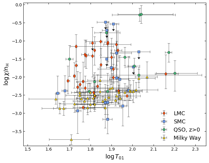
In static equilibrium the temperature of the ISM is determined from the thermal balance of the heating and cooling rates. Consequently in most simplest situation the temperature should depend on the ratio of $\log\chi/n_{\rm H}$ (or $\zeta/n_{\rm H}$, note, that we tight together $\chi$ and $\zeta$). In Fig. 6 we compare the obtained $\chi/n_{\rm H}$ and $T_{01}$ in different samples. Previously, Klimenko & Balashev (2020) reported that observationally $\chi/n_{\rm H}\propto T^{\alpha}$ and actually there may be a correlation between $T_{01}$ and $\chi/n_{\rm H}$, for which we get a power law index $\alpha=1.6^{+1.3}_{-1.1}$ and $2.2^{+1.4}_{-1.3}$ for the LMC and SMC, respectively. However, the correlation is very weak (if it is real) – Pearson correlation coefficients are 0.08 with p-value 0.69 and 0.14 with p-value 0.54 for the LMC and SMC, respectively.
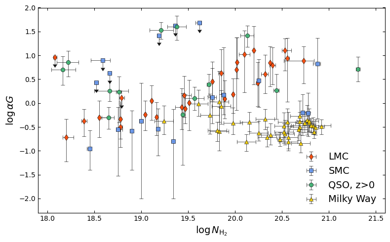
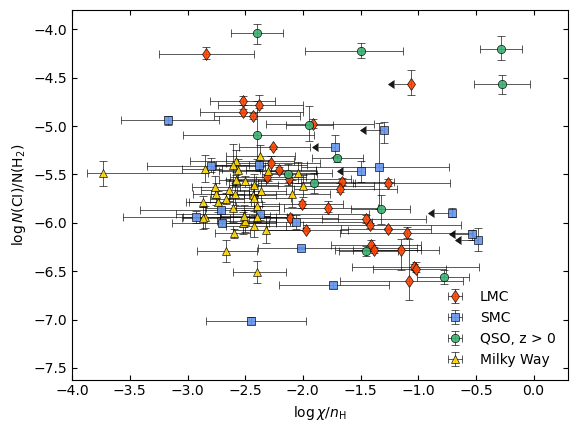
Interestingly, that $\alpha G$ parameter101010Following (Sternberg et al., 2014; Bialy & Sternberg, 2016), $\alpha$ parameter is a ratio of H2 destruction rate (neglecting self-shielding) to the H2 formation rate and $G$ defines the shielding of H2 from UV radiation that was introduced for description of the H i/H2 transition also depends on $\chi/n_{\rm H}$ ratio, apart from the metallicity dependence. Since the metallicities are also constrained in our sample, we provide $\alpha G$ parameter111111To estimate $\alpha G$ parameter we used approximation of Bialy & Sternberg 2016, where we used H2 formation rate to be $R=3\times 10^{-17}\varphi_{\rm g}Z$ cm3s-1, where $\varphi_{\rm g}$ depends on dust properties and close to unity (Sternberg et al., 2014) for the LMC and SMC samples in Tables 3 and 4, respectively. In Fig. 7 we compare the dependence of $\alpha G$ on H2 column densities, measured in different systems. One can see that in case of Magellanic Cloud sample we obtained a large range of $\alpha G$: $\sim 0.2-13$ and $\sim 0.2-50$, for the LMC and SMC, respectively, while in the MW sample it is constrained to lie within $\sim 0.1-1$. Higher values of $\alpha G$ in the LMC and SMC samples are consistent with $\alpha G$ that we measured in the high-redshift systems, $\sim 0.5-40$. This can be connected with a higher value of UV field intensity and lower metallicity in both Magellanic Clouds and distant galaxies, leading to a lower H2 abundance. Interestingly, that we also found a strong correlation of $\alpha G$ parameter with H2 column density in our sample: Pearson correlation coefficients are 0.67 with p-value $2\times 10^{-4}$ and 0.39 with p-value $0.05$ for the LMC and SMC, respectively. This likely indicates that higher H2 column density systems in Magellanic Clouds probe the gas closer to the star-formation regions, where UV field is enhanced. This is directly confirmed by considering estimates of UV field obtained in our sample. On the other hand, Fig. 8 shows that in the LMC and SMC samples, the relative abundance C i/H2 anti-correlates with the strength of UV field, and even more strongly with the ratio of $\chi/n_{\rm H}\propto\alpha G$. The correlation coefficient is $-0.66$ and p-value $2\times 10^{-4}$ for the LMC and $-0.19$ and p-value $0.35$ for the SMC. This is in general in line with chemical models of diffuse ISM (e.g. Wolfire et al., 2008; Liszt, 2015), and will be comprehensively explored in forthcoming paper (Balashev et al. in prep).

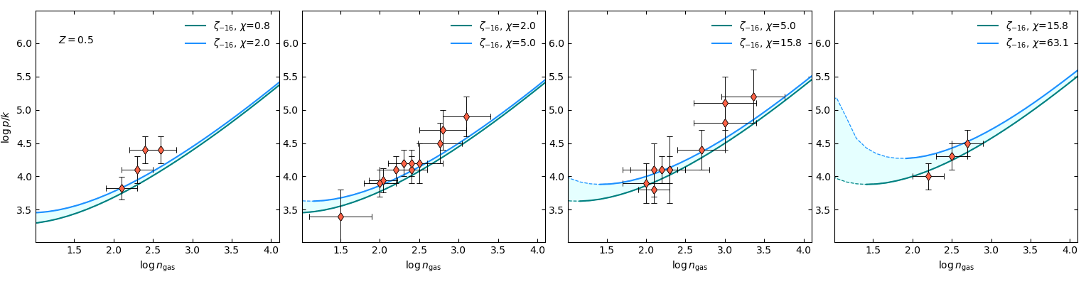
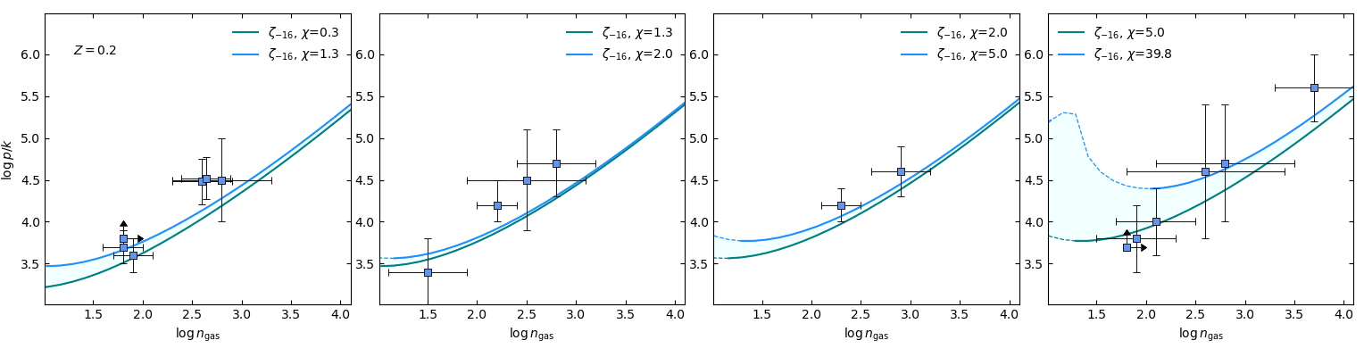
We also show how our estimated results on physical condition are located on the phase diagram of the thermal state of the cold ISM. The phase diagrams for the four bins of $\chi,\zeta$ and associated measured values are shown in Figs 9 and 10, for average values of metallicity in the LMC and SMC, respectively. In fact, to derive $n_{\rm H}$ and $\rm UV$ flux we already used calculation of thermal state using Meudon PDR code. Therefore these phase diagrams are mostly shown for an illustrative purpose only, to highlight that the thermal state of the medium depends on the physical parameters, like $\chi$ and $\zeta$, as well as on the properties and abundance of dust. To calculate the phase diagram we used the same code and similar assumptions on the heating and cooling sources of the medium as it was recently done in Balashev et al. 2022. One can see that our calculations in general agree with Meudon PDR ones that are indirectly reflected by the location of the measured points. On average, Meudon PDR gives slightly higher temperature of the ISM, at lower values of $\chi$ and higher metallicity. This may be due to different scaling of the dust to gas ratio parameter depending on metallicity, the actual behaviour of which is very hard to constrain from observations (see e.g. Rémy-Ruyer et al., 2014).

Refer to caption
Figure 9: Pressure vs density (phase diagram) at the metallicity $Z=0.5$, corresponding to the mean LMC metallicity. Data is divided into four bins relative to UV field intensity. The solid lines and the light-blue shaded area show model curves calculated respectively to the bins and indicated in the legend. Red diamonds are values obtained for the LMC.
Refer to caption
Figure 10: Pressure vs density (phase diagram) for the metallicity $Z=0.2$, corresponding to the mean SMC metallicity. The graphic description is the same as in Fig. 9. Blue squares are values obtained for the SMC.

7 Summary

Using HST archival data we analysed C i  absorption lines and obtained populations of fine-structure levels in 21 and 23 systems in the LMC and SMC, respectively. In the most of these systems we also analysed metal lines and measured metallicities to be $\log Z=-0.66\pm 0.22$ and $-0.99\pm 0.19$ (providing an average value and standard deviation) for the LMC and SMC, respectively.

Using the obtained C i fine-structure level populations and populations of H2 rotational levels previously reported in accompanying paper (Kosenko & Balashev, 2023) we constrained physical conditions in the systems, namely, hydrogen gas density and UV field intensity (or cosmic ray ionization rate assumed to be coscaled with UV field). The average values of hydrogen gas densities are $\log n_{\rm H}\sim 2.5$ and $\log n_{\rm H}\sim 2.6$, with standard deviation 0.4 and 0.6, for the LMC and SMC, respectively. The mean intensities of UV field are $\log\chi_{\rm LMC}\sim 0.7$ and $\log\chi_{\rm SMC}\sim 0.3$ (in units of Mathis field) with standard deviation of 0.4 and 0.5, for the LMC and SMC, respectively. We also estimated the average thermal pressure in our sample to be $\log p_{\rm LMC}\sim 4.2$ and $\log p_{\rm SMC}\sim 4.3$ with standard deviation 0.4 and 0.5 for the LMC and SMC, respectively.

We compared the obtained hydrogen gas densities and thermal pressures in Magellanic Clouds with measurements in the Milky-Way and high-$z$ DLAs. The average thermal pressure in Magellanic Clouds is half an order of magnitude higher than thermal pressure measured in C i absorption systems in the Milky-Way $\log p_{\rm MW}\sim 3.7\pm 0.2$. Such high values of thermal pressure were observed in strong CO-bearing MW clouds (Welty et al., 2020; Federman et al., 2021), which represent translucent/dense phase of the ISM. This difference can be explained by lower metallicities and higher UV field/CRIR intensity in the Magellanic Clouds than in the MW samples, which is directly confirmed by our data and in line with previous studies (e.g. Bernard et al., 2008; Welty et al., 2016). In that sense, Magellanic Clouds absorption systems probe ISM at sufficiently different regime than MW do and provide interesting test-case for the studies of high redshift galaxies. This also agree with some similarities of obtain physical parameters in the Magellanic Clouds and high redshift absorption systems, although the latter likely predominantly probe an outskirts of the galaxies due to their higher cross section.

Data availability

The results of this paper are based on open data retrieved from the FUSE and HST telescope archives. These data can be shared on reasonable requests to the authors.

Acknowledgements

This work was supported by RSF grant 23-12-00166.

References

  • Abgrall et al. (1992) Abgrall H., Le Bourlot J., Pineau Des Forets G., Roueff E., Flower D. R., Heck L., 1992, A&A, 253, 525
  • Anders & Grevesse (1989) Anders E., Grevesse N., 1989, Geochimica Cosmochimica Acta, 53, 197
  • André et al. (2004) André M. K., et al., 2004, A&A, 422, 483
  • Asplund et al. (2009) Asplund M., Grevesse N., Sauval A. J., Scott P., 2009, ARA&A, 47, 481
  • Balashev et al. (2009) Balashev S. A., Varshalovich D. A., Ivanchik A. V., 2009, Astronomy Letters, 35, 150
  • Balashev et al. (2017) Balashev S. A., et al., 2017, MNRAS, 470, 2890
  • Balashev et al. (2019) Balashev S. A., et al., 2019, MNRAS, 490, 2668
  • Balashev et al. (2020) Balashev S. A., Ledoux C., Noterdaeme P., Srianand R., Petitjean P., Gupta N., 2020, MNRAS, 497, 1946
  • Balashev et al. (2022) Balashev S. A., Telikova K. N., Noterdaeme P., 2022, MNRAS, 509, L26
  • Bernard et al. (2008) Bernard J.-P., et al., 2008, AJ, 136, 919
  • Bialy & Sternberg (2016) Bialy S., Sternberg A., 2016, ApJ, 822, 83
  • Bialy & Sternberg (2019) Bialy S., Sternberg A., 2019, ApJ, 881, 160
  • Blair et al. (2009) Blair W. P., Oliveira C., LaMassa S., Gutman S., Danforth C. W., Fullerton A. W., Sankrit R., Gruendl R., 2009, PASP, 121, 634
  • Bluhm & de Boer (2001) Bluhm H., de Boer K. S., 2001, A&A, 379, 82
  • Burgh et al. (2010) Burgh E. B., France K., Jenkins E. B., 2010, ApJ, 708, 334
  • De Cia et al. (2018) De Cia A., Ledoux C., Petitjean P., Savaglio S., 2018, A&A, 611, A76
  • De Cia et al. (2021) De Cia A., Jenkins E. B., Fox A. J., Ledoux C., Ramburuth-Hurt T., Konstantopoulou C., Petitjean P., Krogager J.-K., 2021, Nature, 597, 206
  • Federman et al. (2021) Federman S. R., et al., 2021, ApJ, 914, 59
  • Gillmon et al. (2006) Gillmon K., Shull J. M., Danforth C., Tumlinson J., 2006, in Sonneborn G., Moos H. W., Andersson B. G., eds, Astronomical Society of the Pacific Conference Series Vol. 348, Astrophysics in the Far Ultraviolet: Five Years of Discovery with FUSE. p. 439
  • Goodman & Weare (2010) Goodman J., Weare J., 2010, Communications in Applied Mathematics and Computational Science, 5, 65
  • Graczyk et al. (2020) Graczyk D., et al., 2020, ApJ, 904, 13
  • Green et al. (2012) Green J. C., et al., 2012, ApJ, 744, 60
  • Jenkins & Tripp (2001) Jenkins E. B., Tripp T. M., 2001, ApJS, 137, 297
  • Jenkins & Tripp (2011) Jenkins E. B., Tripp T. M., 2011, ApJ, 734, 65
  • Jenkins & Tripp (2021) Jenkins E. B., Tripp T. M., 2021, ApJ, 916, 17
  • Jenkins & Wallerstein (2017) Jenkins E. B., Wallerstein G., 2017, ApJ, 838, 85
  • Jorgenson et al. (2009) Jorgenson R. A., Wolfe A. M., Prochaska J. X., Carswell R. F., 2009, ApJ, 704, 247
  • Jorgenson et al. (2010) Jorgenson R. A., Wolfe A. M., Prochaska J. X., 2010, ApJ, 722, 460
  • Klimenko & Balashev (2020) Klimenko V. V., Balashev S. A., 2020, MNRAS, 498, 1531
  • Kosenko & Balashev (2023) Kosenko D. N., Balashev S. A., 2023, MNRAS, p. stad2299
  • Kosenko et al. (2021) Kosenko D. N., Balashev S. A., Noterdaeme P., Krogager J. K., Srianand R., Ledoux C., 2021, MNRAS, 505, 3810
  • Krogager & Noterdaeme (2020) Krogager J.-K., Noterdaeme P., 2020, A&A, 644, L6
  • Krogager et al. (2017) Krogager J. K., Møller P., Fynbo J. P. U., Noterdaeme P., 2017, MNRAS, 469, 2959
  • Le Petit et al. (2006) Le Petit F., Nehmé C., Le Bourlot J., Roueff E., 2006, ApJS, 164, 506
  • Ledoux et al. (2003) Ledoux C., Petitjean P., Srianand R., 2003, MNRAS, 346, 209
  • Liszt (2015) Liszt H. S., 2015, ApJ, 799, 66
  • Mathis et al. (1983) Mathis J. S., Mezger P. G., Panagia N., 1983, A&A, 128, 212
  • Moos et al. (2000) Moos H. W., et al., 2000, ApJ, 538, L1
  • Muzahid et al. (2015) Muzahid S., Srianand R., Charlton J., 2015, MNRAS, 448, 2840
  • Niemela & Morrell (1986) Niemela V. S., Morrell N. I., 1986, ApJ, 310, 715
  • Noterdaeme et al. (2018) Noterdaeme P., Ledoux C., Zou S., Petitjean P., Srianand R., Balashev S., López S., 2018, A&A, 612, A58
  • Ostrov & Lapasset (2003) Ostrov P. G., Lapasset E., 2003, MNRAS, 338, 141
  • Pietrzyński et al. (2019) Pietrzyński G., et al., 2019, Nature, 567, 200
  • Rachford et al. (2002) Rachford B. L., et al., 2002, ApJ, 577, 221
  • Rachford et al. (2009) Rachford B. L., et al., 2009, ApJS, 180, 125
  • Ranjan et al. (2018) Ranjan A., et al., 2018, A&A, 618, A184
  • Ranjan et al. (2020) Ranjan A., Noterdaeme P., Krogager J. K., Petitjean P., Srianand R., Balashev S. A., Gupta N., Ledoux C., 2020, A&A, 633, A125
  • Rémy-Ruyer et al. (2014) Rémy-Ruyer A., et al., 2014, A&A, 563, A31
  • Ritchey et al. (2023) Ritchey A. M., Jenkins E. B., Shull J. M., Savage B. D., Federman S. R., Lambert D. L., 2023, arXiv e-prints, p. arXiv:2301.09743
  • Roman-Duval et al. (2019) Roman-Duval J., et al., 2019, ApJ, 871, 151
  • Roman-Duval et al. (2021) Roman-Duval J., et al., 2021, ApJ, 910, 95
  • Russell & Dopita (1992) Russell S. C., Dopita M. A., 1992, ApJ, 384, 508
  • Sahnow et al. (2000) Sahnow D. J., et al., 2000, ApJ, 538, L7
  • Sandstrom et al. (2010) Sandstrom K. M., Bolatto A. D., Draine B. T., Bot C., Stanimirović S., 2010, ApJ, 715, 701
  • Savage et al. (1977) Savage B. D., Bohlin R. C., Drake J. F., Budich W., 1977, ApJ, 216, 291
  • Shull et al. (2021) Shull J. M., Danforth C. W., Anderson K. L., 2021, ApJ, 911, 55
  • Srianand et al. (2005) Srianand R., Petitjean P., Ledoux C., Ferland G., Shaw G., 2005, MNRAS, 362, 549
  • Sternberg et al. (2014) Sternberg A., Le Petit F., Roueff E., Le Bourlot J., 2014, ApJ, 790, 10
  • Tchernyshyov et al. (2015) Tchernyshyov K., Meixner M., Seale J., Fox A., Friedman S. D., Dwek E., Galliano F., 2015, ApJ, 811, 78
  • Telikova et al. (2022) Telikova K. N., Balashev S. A., Noterdaeme P., Krogager J. K., Ranjan A., 2022, MNRAS, 510, 5974
  • Welty et al. (2012) Welty D. E., Xue R., Wong T., 2012, ApJ, 745, 173
  • Welty et al. (2016) Welty D. E., Lauroesch J. T., Wong T., York D. G., 2016, ApJ, 821, 118
  • Welty et al. (2020) Welty D. E., Sonnentrucker P., Snow T. P., York D. G., 2020, ApJ, 897, 36
  • Wolfire et al. (2008) Wolfire M. G., Tielens A. G. G. M., Hollenbach D., Kaufman M. J., 2008, ApJ, 680, 384
  • Woodgate et al. (1998) Woodgate B. E., et al., 1998, PASP, 110, 1183

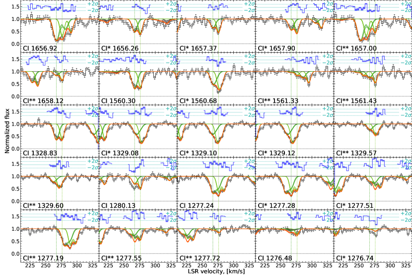
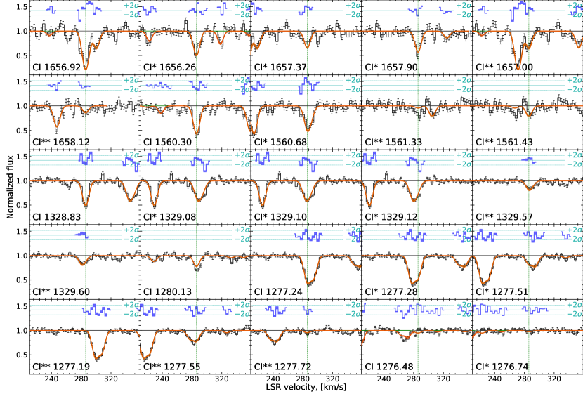
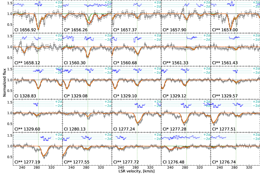
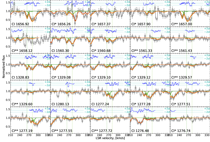
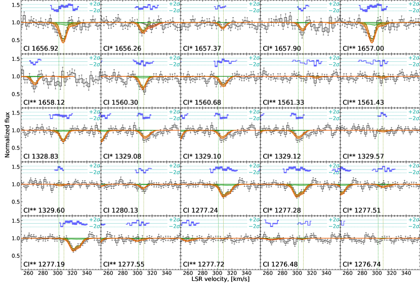
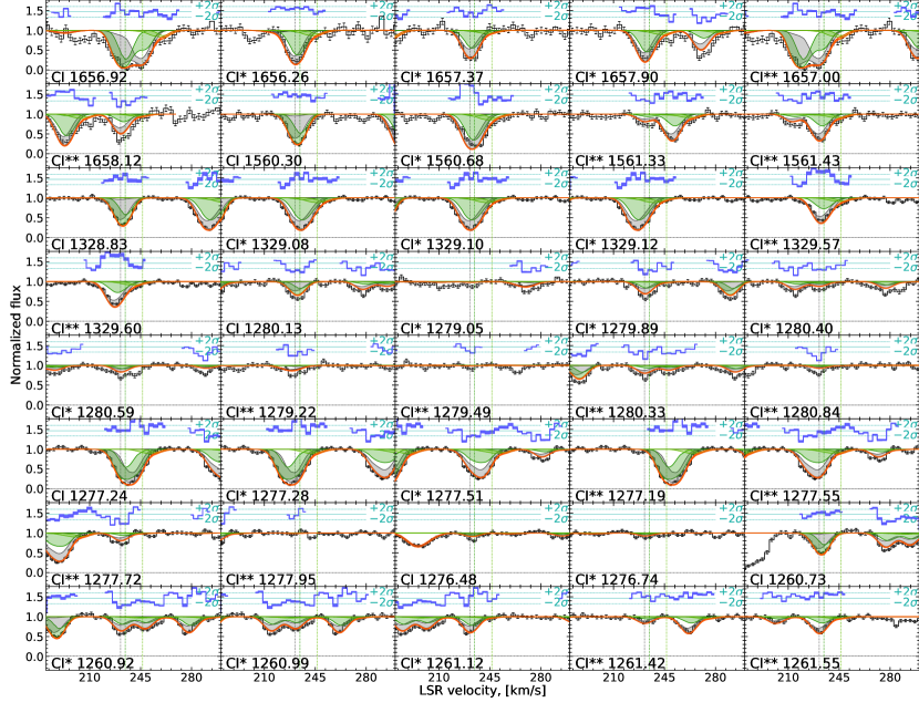
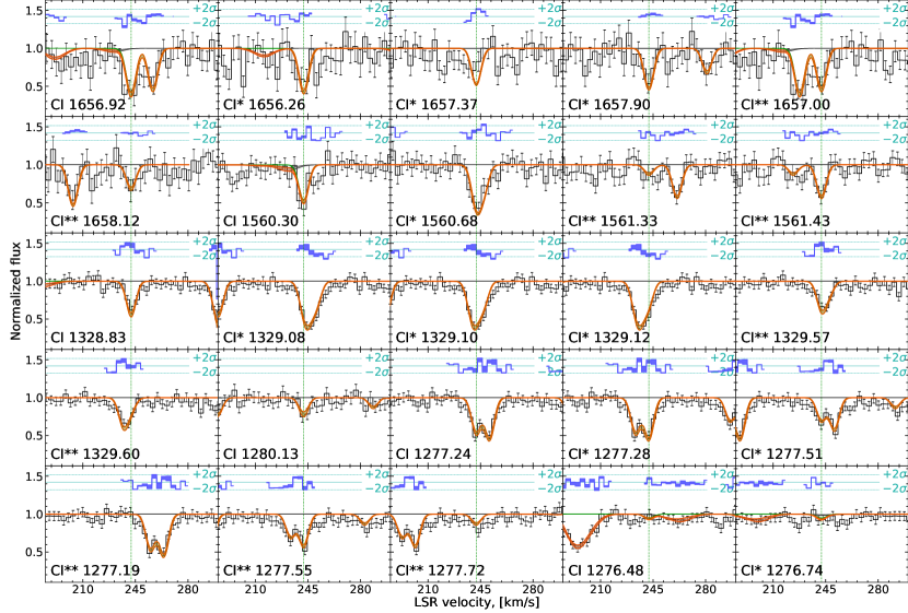
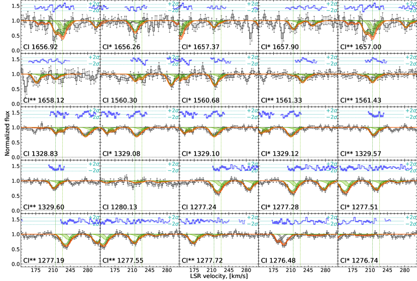
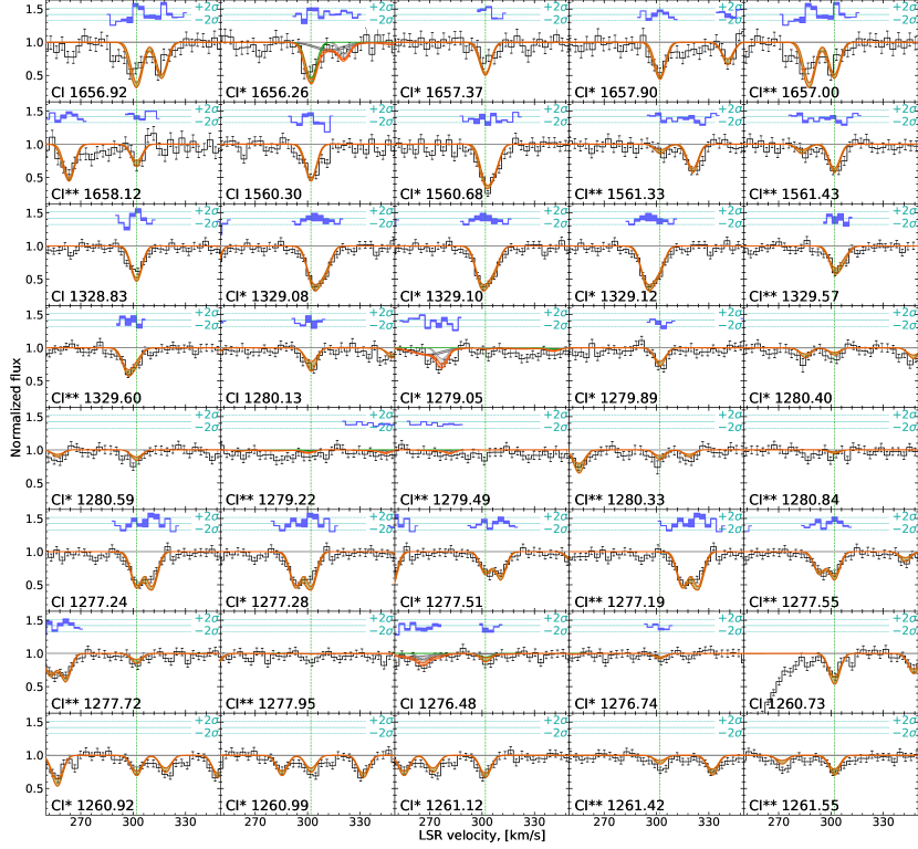
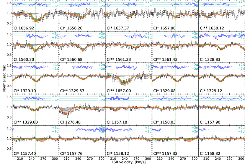
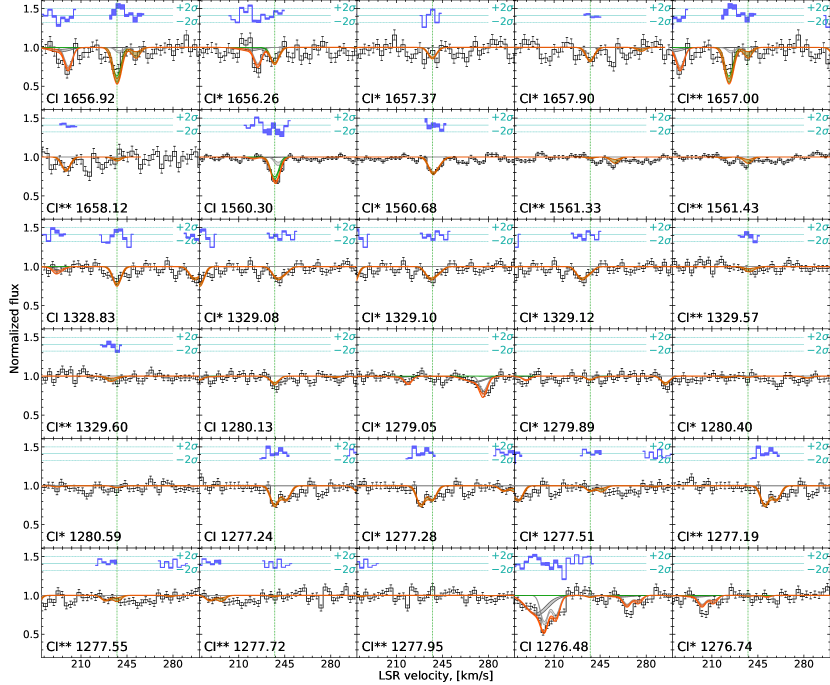
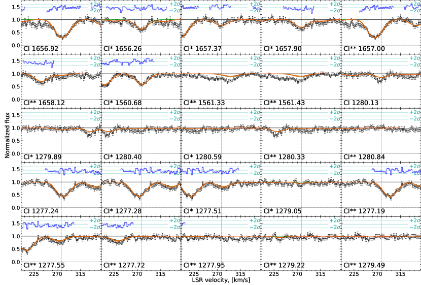
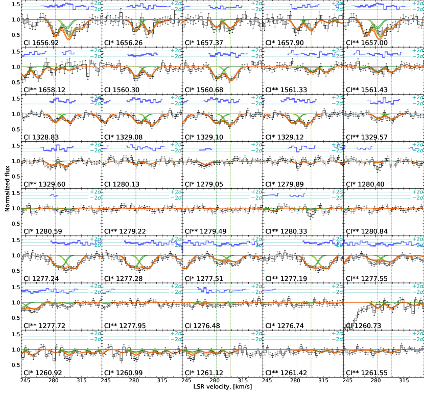
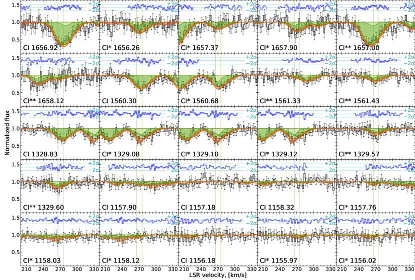
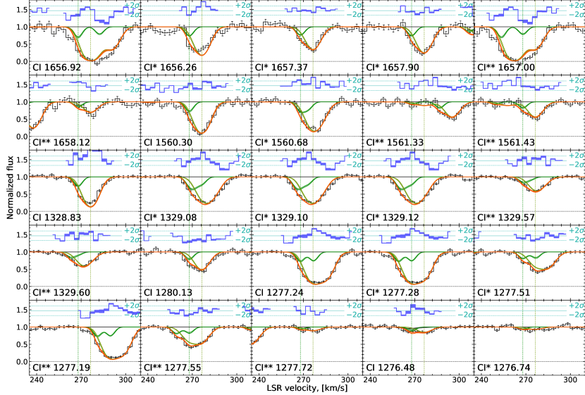
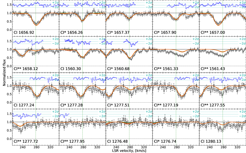
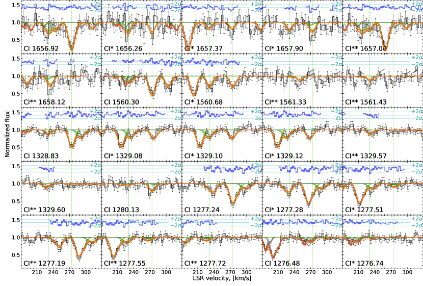
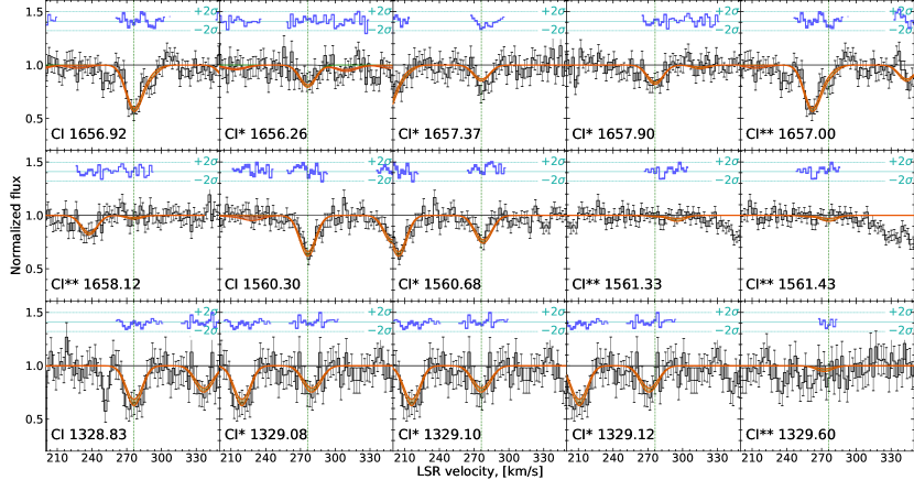
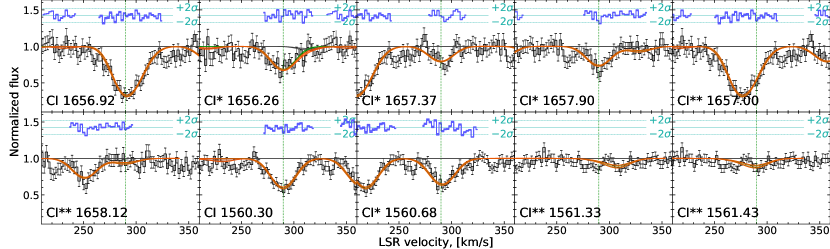
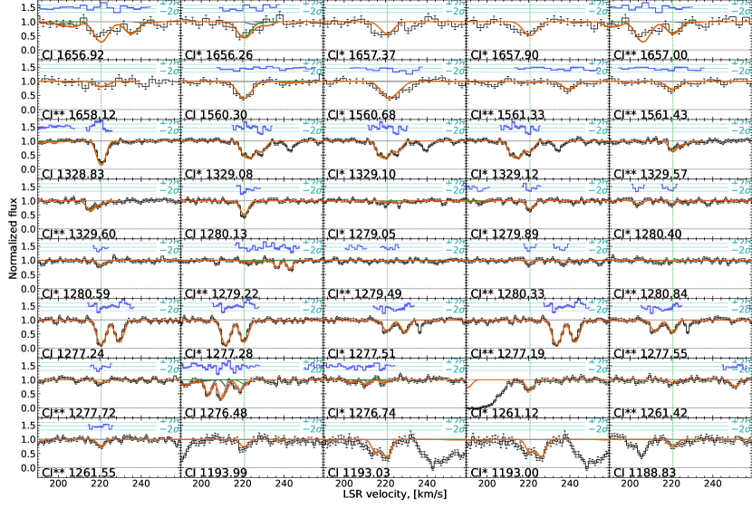
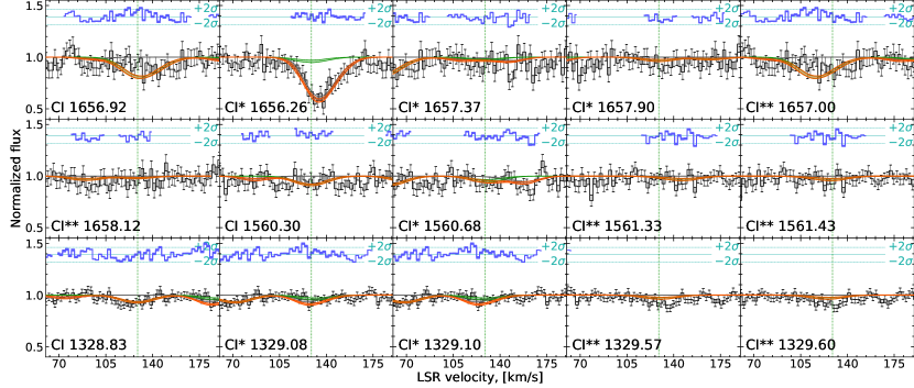
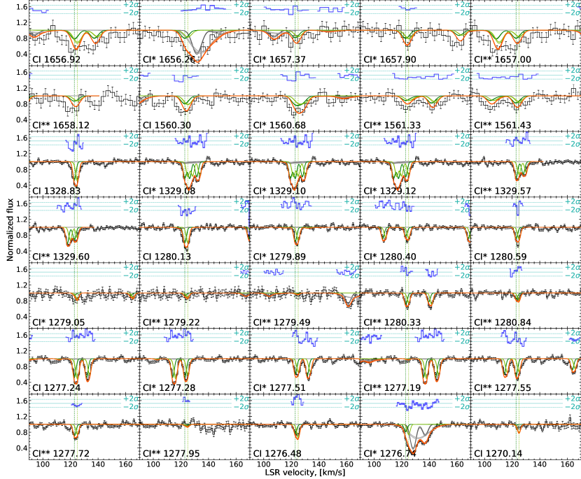
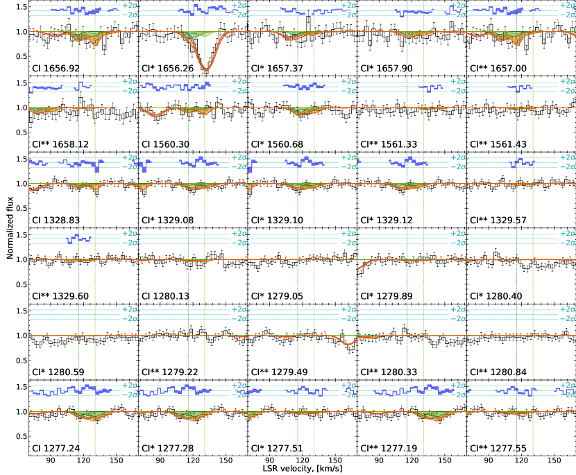
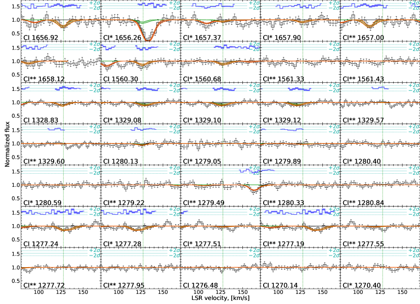
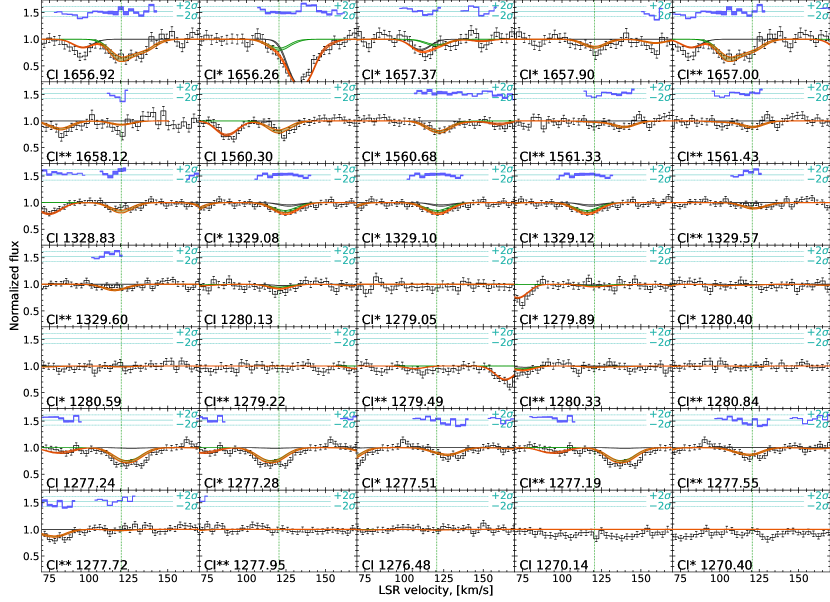
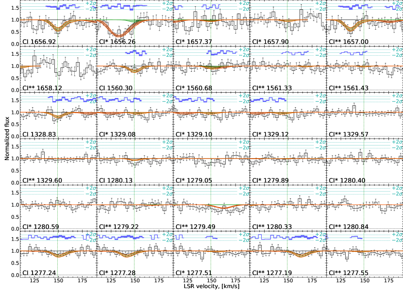
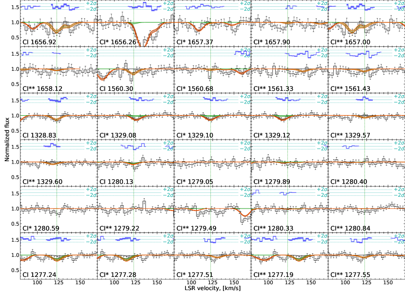
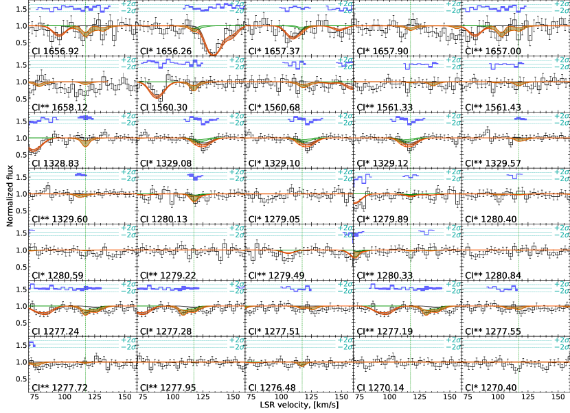
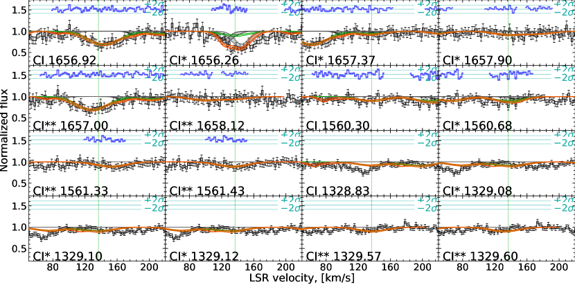
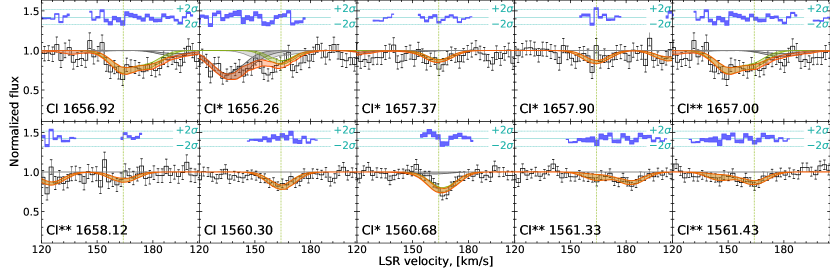
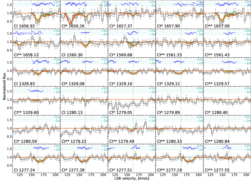
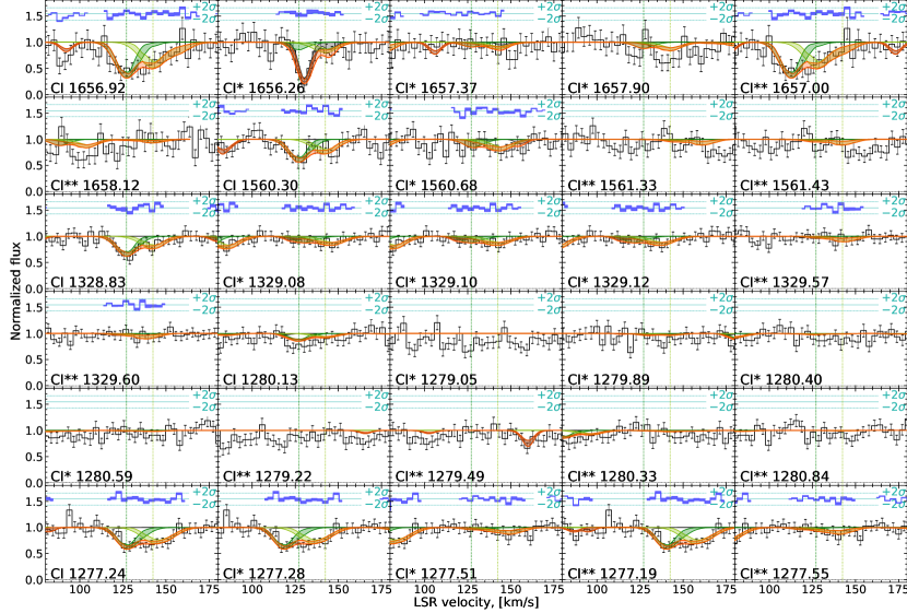
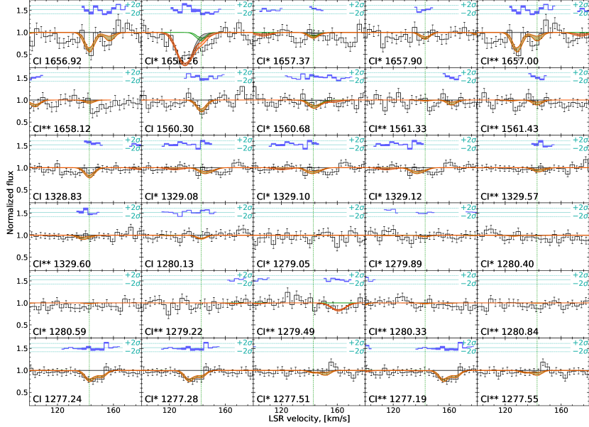
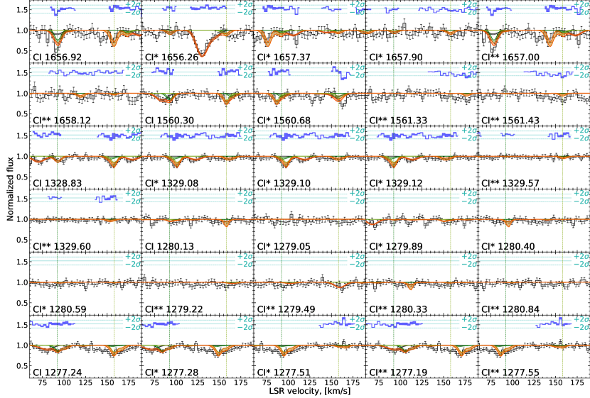
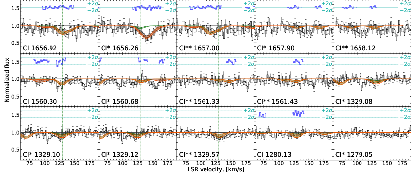
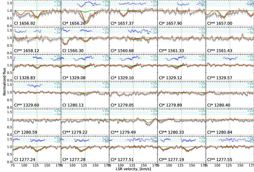
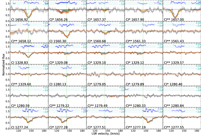
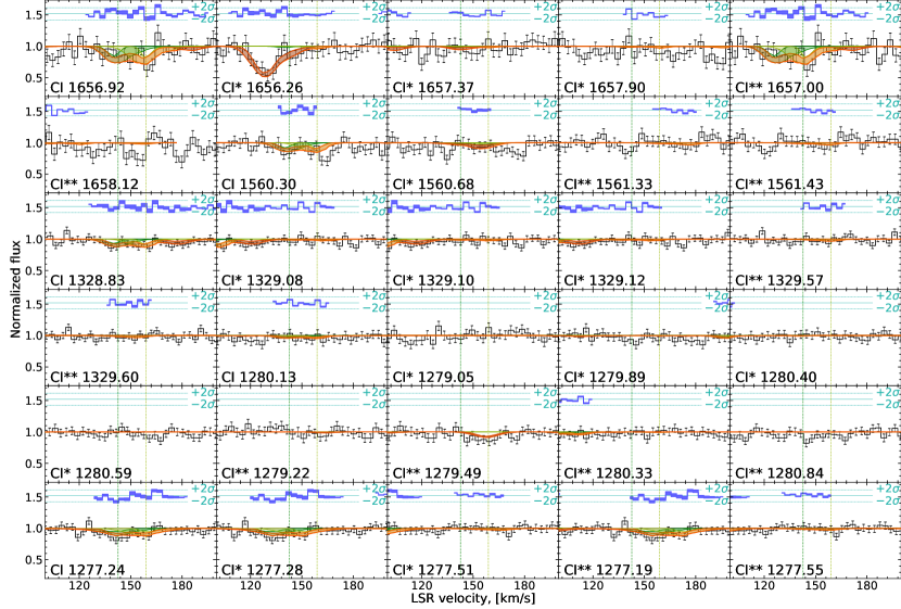
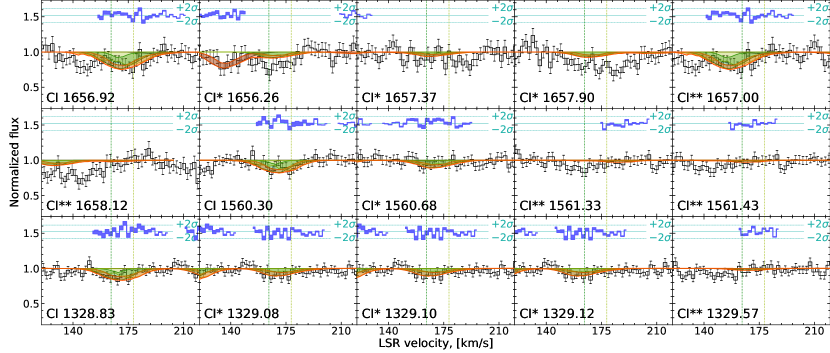
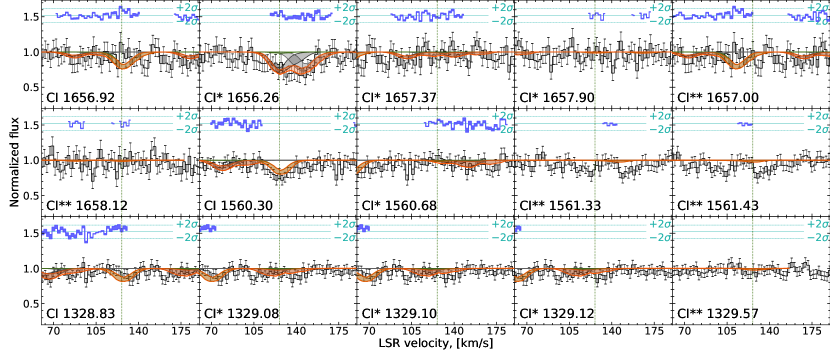
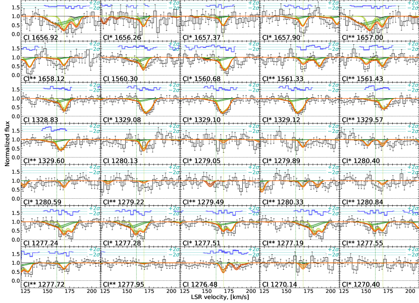
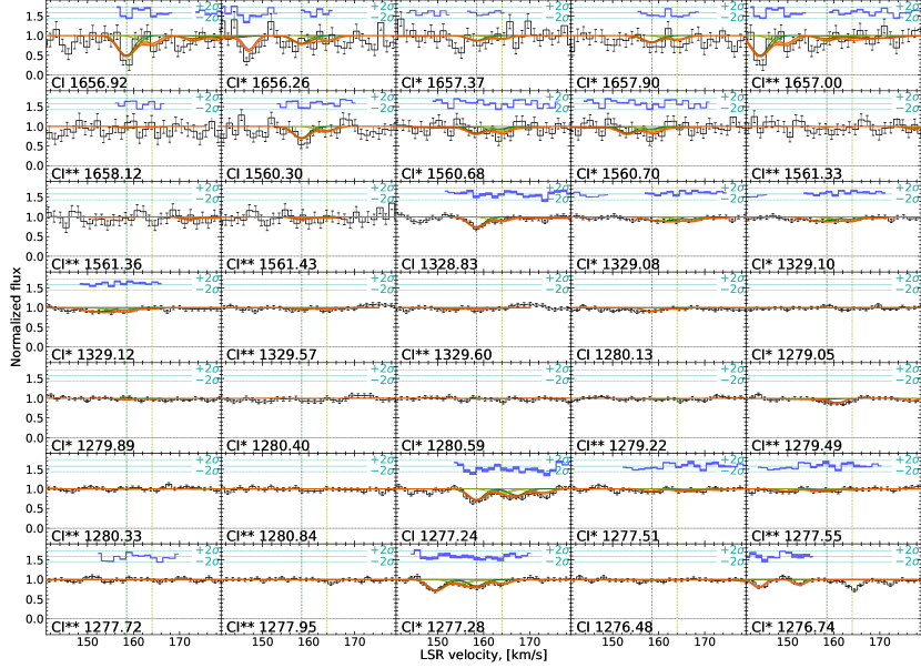
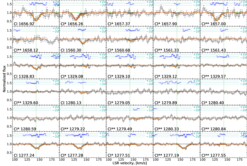
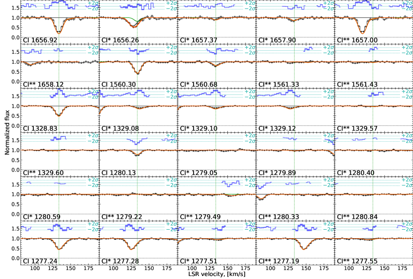
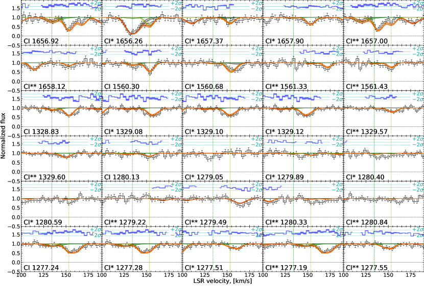
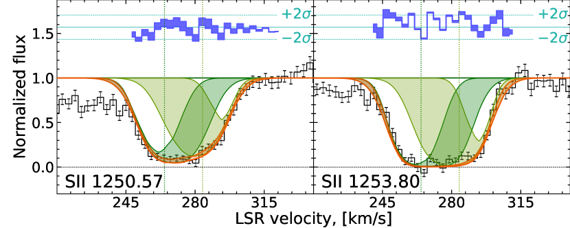
Appendix A Details on C i  fit

In this section we show fit of the C i  absorption lines in each system. Here we do not show fully blended (e.g. C i1560.70, C i∗∗ 1561.36) and the most weak lines.

A.1 Large Magellanic Cloud

Refer to caption
Figure 11: C i  absorption lines fit in the system towards Sk-67 2 in the LMC. Here black line show spectrum, coloured bands show synthetic spectrum, sampled from 0.683 credible interval of the posterior probability distribution of the fitting parameters. Red line represent total line profile, while grey and green lines show Milky Way and Magellanic Cloud components, respectively. Blue points at the top of each panel show residuals. Here we show only components found in the Magellanic Clouds.
Refer to caption
Figure 12: C i  absorption lines fit in the system towards Sk-67 5 in the LMC. Lines are the same as in Figure 11.
Refer to caption
Figure 13: C i  absorption lines fit in the system towards Sk-67 20 in the LMC. Lines are the same as in Figure 11.
Refer to caption
Figure 14: C i  absorption lines fit in the system towards PGMW 3070 in the LMC. Lines are the same as in Figure 11.
Refer to caption
Figure 15: C i  absorption lines fit in the system towards LH10 3120 in the LMC. Lines are the same as in Figure 11.
Refer to caption
Figure 16: C i  absorption lines fit in the system towards PGMW 3223in the LMC. Lines are the same as in Figure 11.
Refer to caption
Figure 17: C i  absorption lines fit in the system towards Sk-66 35 in the LMC. Lines are the same as in Figure 11.
Refer to caption
Figure 18: C i  absorption lines fit in the system towards Sk-66 51 in the LMC. Lines are the same as in Figure 11.
Refer to caption
Figure 19: C i  absorption lines fit in the system towards Sk-70 79 in the LMC. Lines are the same as in Figure 11.
Refer to caption
Figure 20: C i  absorption lines fit in the system towards Sk-68 52 in LMC. Lines are the same as in Figure 11.
Refer to caption
Figure 21: C i  absorption lines fit in the system towards Sk-71 8 in the LMC. Lines are the same as in Figure 11.
Refer to caption
Figure 22: C i  absorption lines fit in the system towards Sk-69 106 in the LMC. Lines are the same as in Figure 11.
Refer to caption
Figure 23: C i  absorption lines fit in the system towards Sk-68 73 in the LMC. Lines are the same as in Figure 11.
Refer to caption
Figure 24: C i  absorption lines fit in the system towards Sk-67 105 in LMC. Lines are the same as in Figure 11.
Refer to caption
Figure 25: C i  absorption lines fit in the system towards BI 184 in the LMC. Lines are the same as in Figure 11.
Refer to caption
Figure 26: C i  absorption lines fit in the system towards Sk-71 45 in the LMC. Lines are the same as in Figure 11.
Refer to caption
Figure 27: C i  absorption lines fit in the system towards Sk-71 46 in LMC. Lines are the same as in Figure 11.
Refer to caption
Figure 28: C i  absorption lines fit in the system towards Sk-69 191 in LMC. Lines are the same as in Figure 11.
Refer to caption
Figure 29: C i  absorption lines fit in the system towards BI 237 in the LMC. Lines are the same as in Figure 11.
Refer to caption
Figure 30: C i  absorption lines fit in the system towards Sk-68 129 in the LMC. Lines are the same as in Figure 11.
Refer to caption
Figure 31: C i  absorption lines fit in the system towards Sk-66 172 in LMC. Lines are the same as in Figure 11.
Refer to caption
Figure 32: C i  absorption lines fit in the system towards BI 253 in the LMC. Lines are the same as in Figure 11.
Refer to caption
Figure 33: C i  absorption lines fit in the system towards Sk-68 135 in the LMC. Lines are the same as in Figure 11.
Refer to caption
Figure 34: C i  absorption lines fit in the system towards Sk-69 246 in the LMC. Lines are the same as in Figure 11.
Refer to caption
Figure 35: C i  absorption lines fit in the system towards Sk-68 140 in the LMC. Lines are the same as in Figure 11.
Refer to caption
Figure 36: C i  absorption lines fit in the system towards Sk-71 50 in the LMC. Lines are the same as in Figure 11.
Refer to caption
Figure 37: C i  absorption lines fit in the system towards Sk-71 50 in the LMC. Lines are the same as in Figure 11.
Refer to caption
Figure 38: C i  absorption lines fit in the system towards Sk-69 279 in LMC. Lines are the same as in Figure 11.
Refer to caption
Figure 39: C i  absorption lines fit in the system towards Sk-68 155 in LMC. Lines are the same as in Figure 11.
Refer to caption
Figure 40: C i  absorption lines fit in the system towards Sk-70 115 in the LMC. Lines are the same as in Figure 11.

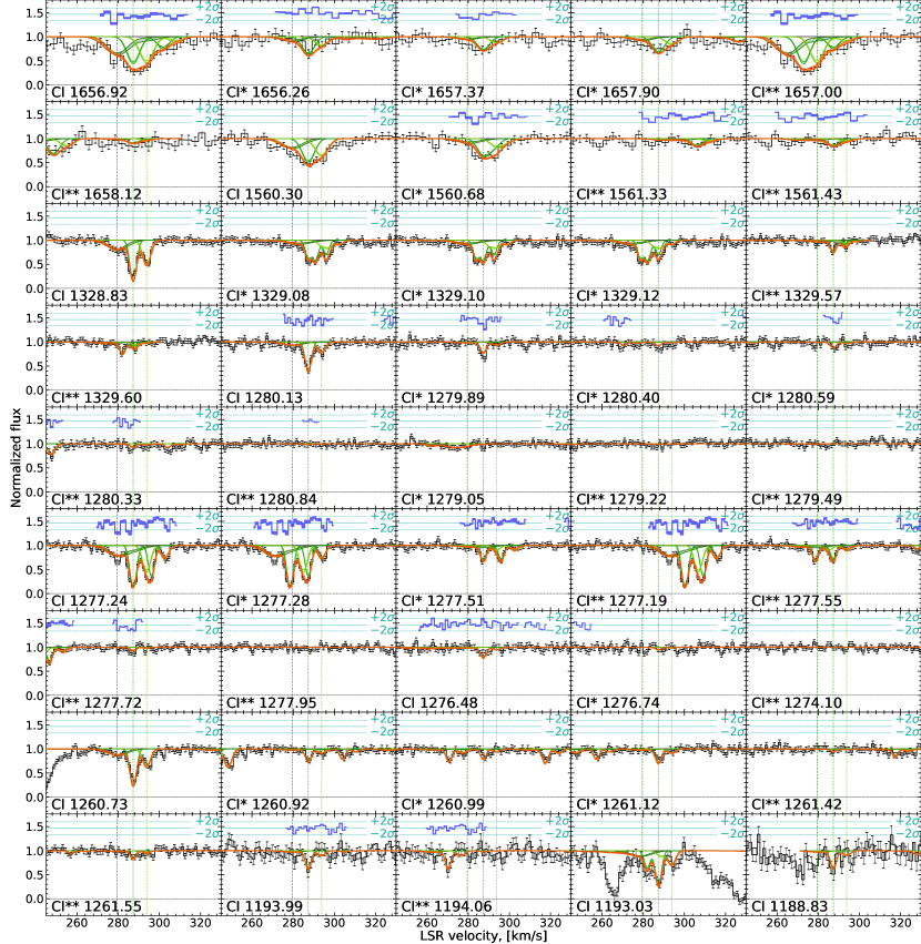
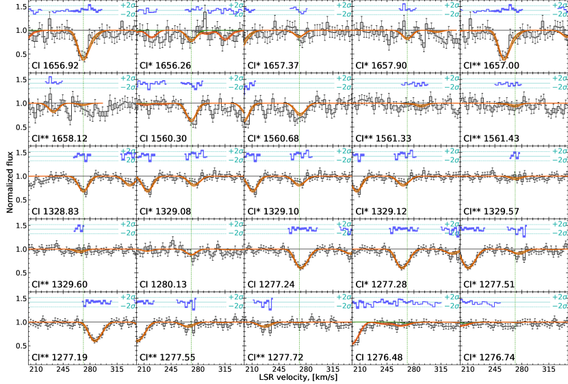
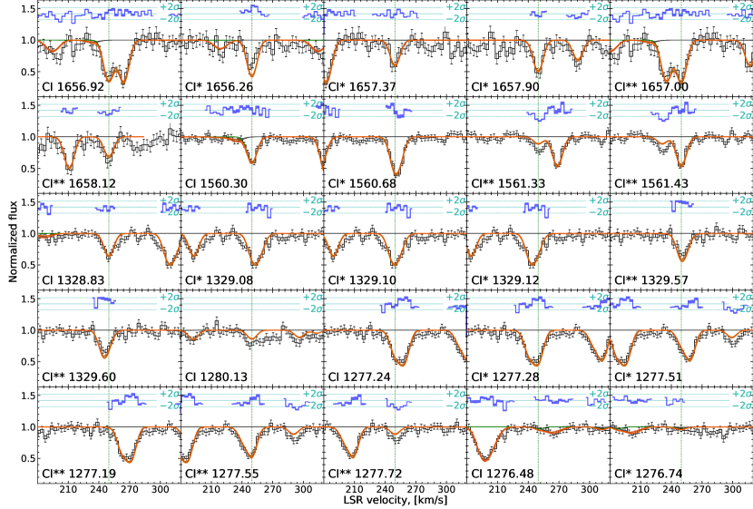
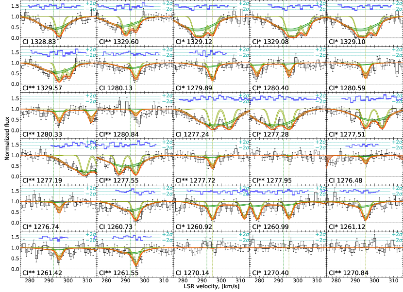
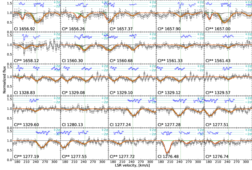
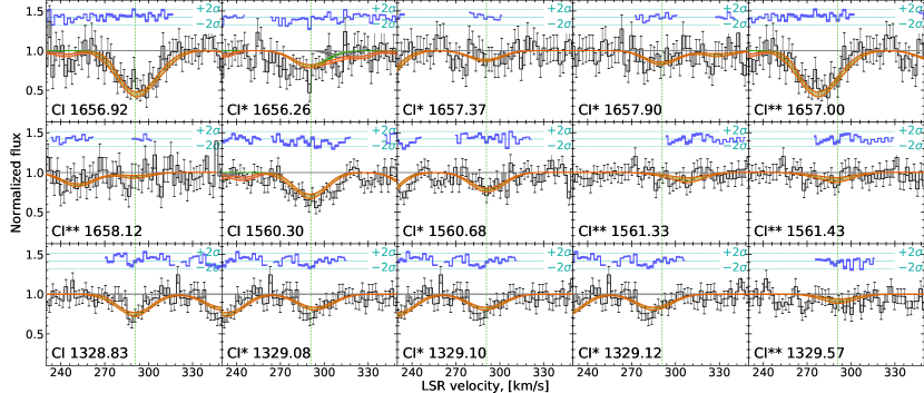
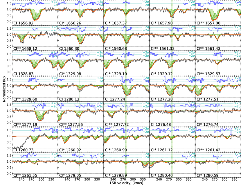
A.2 Small Magellanic Cloud
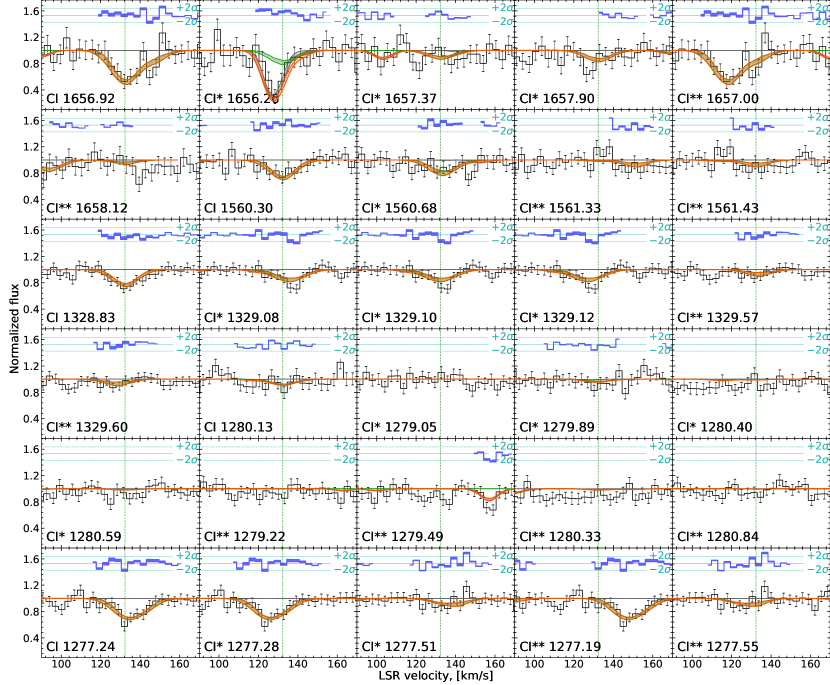
Refer to caption
Figure 41: C i  absorption lines fit in the system towards AV 6 in the SMC. Lines are the same as in Figure 11
Refer to caption
Figure 42: C i  absorption lines fit in the system towards AV 15 in the SMC. Lines are the same as in Figure 11
Refer to caption
Figure 43: C i  absorption lines fit in the system towards AV 26 in the SMC. Lines are the same as in Figure 11
Refer to caption
Figure 44: C i  absorption lines fit in the system towards AV 47 in the SMC. Lines are the same as in Figure 11
Refer to caption
Figure 45: C i  absorption lines fit in the system towards AV 69 in SMC. Lines are the same as in Figure 11
Refer to caption
Figure 46: C i  absorption lines fit in the system towards AV 75 in the SMC. Lines are the same as in Figure 11
Refer to caption
Figure 47: C i  absorption lines fit in the system towards AV 80 in the SMC. Lines are the same as in Figure 11
Refer to caption
Figure 48: C i  absorption lines fit in the system towards AV 81 in the SMC. Lines are the same as in Figure 11
Refer to caption
Figure 49: C i  absorption lines fit in the system towards AV 95 in SMC. Lines are the same as in Figure 11
Refer to caption
Figure 50: C i  absorption lines fit in the system towards AV 104 in the SMC. Lines are the same as in Figure 11
[Uncaptioned image]

captionC i  absorption lines fit in the system towards AV 170 in the SMC. Lines are the same as in Figure 11

Refer to caption
Figure 51: C i  absorption lines fit in the system towards AV 175 in the SMC. Lines are the same as in Figure 11
Refer to caption
Figure 52: C i  absorption lines fit in the system towards AV 207 in SMC. Lines are the same as in Figure 11
Refer to caption
Figure 53: C i  absorption lines fit in the system towards AV 210 in the SMC. Lines are the same as in Figure 11
Refer to caption
Figure 54: C i  absorption lines fit in the system towards AV 215 in the SMC. Lines are the same as in Figure 11
Refer to caption
Figure 55: C i  absorption lines fit in the system towards AV 216 in the SMC. Lines are the same as in Figure 11
Refer to caption
Figure 56: C i  absorption lines fit in the system towards AV 242 in SMC. Lines are the same as in Figure 11
Refer to caption
Figure 57: C i  absorption lines fit in the system towards AV 243 in SMC. Lines are the same as in Figure 11
Refer to caption
Figure 58: C i  absorption lines fit in the system towards AV 266 in the SMC. Lines are the same as in Figure 11
Refer to caption
Figure 59: C i  absorption lines fit in the system towards AV 372 in the SMC. Lines are the same as in Figure 11
Refer to caption
Figure 60: C i  absorption lines fit in the system towards AV 423 in SMC. Lines are the same as in Figure 11
Refer to caption
Figure 61: C i  absorption lines fit in the system towards AV 440 in SMC. Lines are the same as in Figure 11
Refer to caption
Figure 62: C i  absorption lines fit in the system towards AV 472 in the SMC. Lines are the same as in Figure 11
Refer to caption
Figure 63: C i  absorption lines fit in the system towards AV 476 in the SMC. Lines are the same as in Figure 11
Refer to caption
Figure 64: C i  absorption lines fit in the system towards AV 479 in the SMC. Lines are the same as in Figure 11
Refer to caption
Figure 65: C i  absorption lines fit in the system towards AV 488 in SMC. Lines are the same as in Figure 11
Refer to caption
Figure 66: C i  absorption lines fit in the system towards AV 490 in the SMC. Lines are the same as in Figure 11
Refer to caption
Figure 67: C i  absorption lines fit in the system towards Sk 191 in the SMC. Lines are the same as in Figure 11

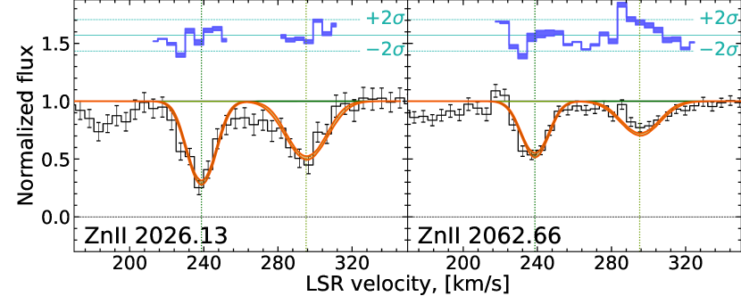
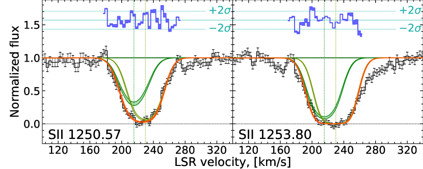
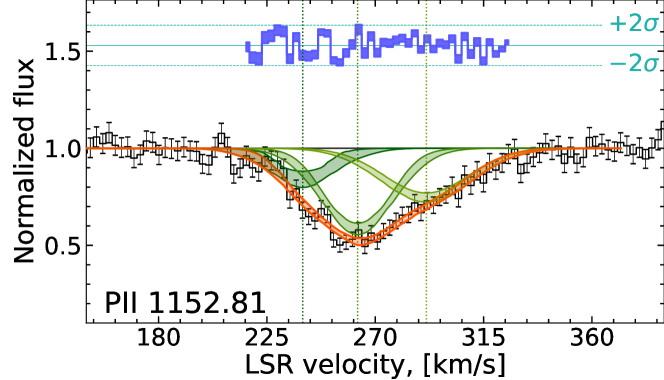
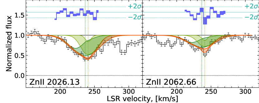
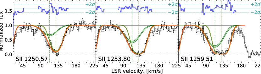
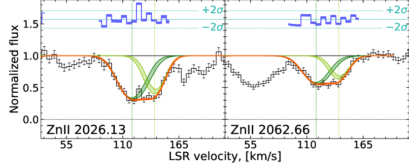
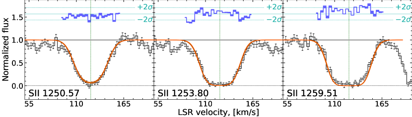
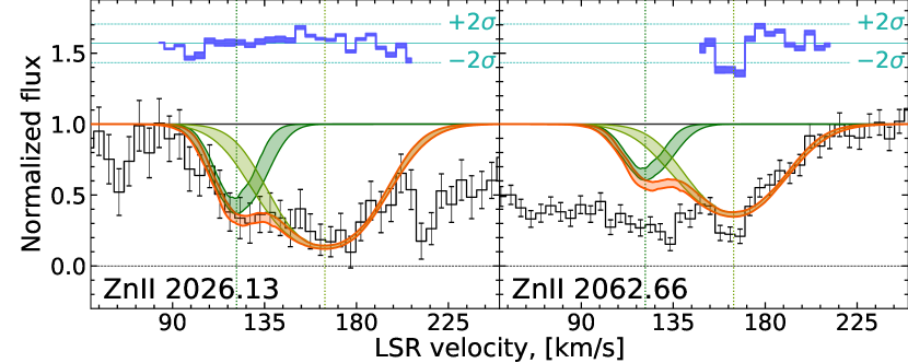
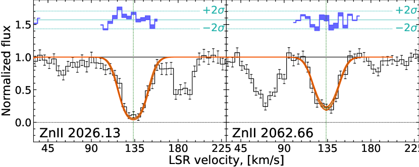
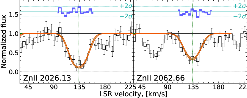
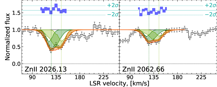
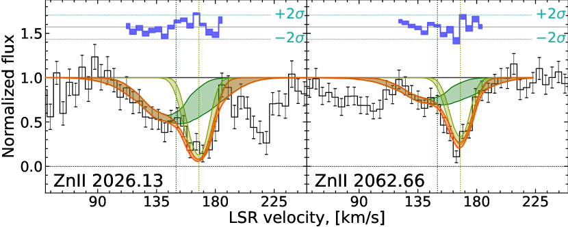
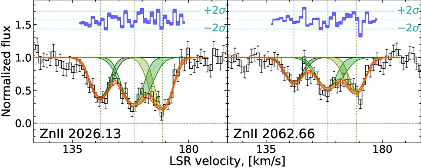
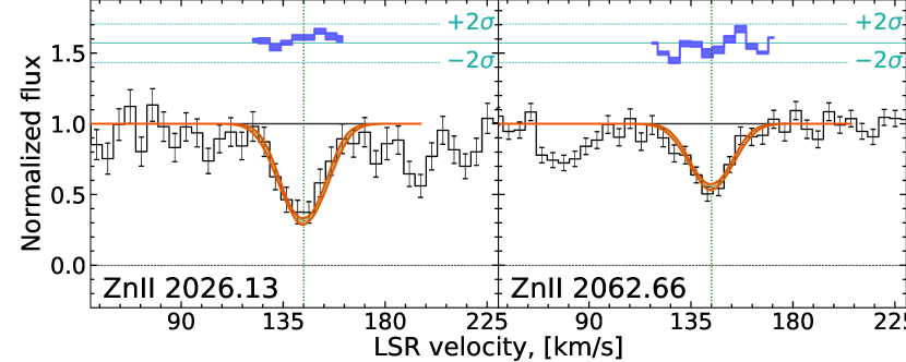
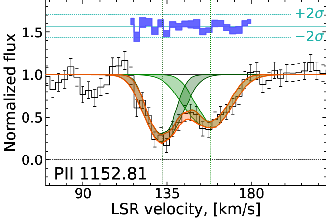
Appendix B Details on metal lines fit

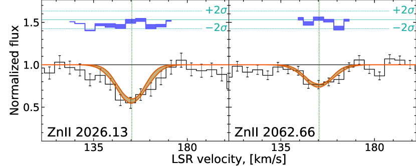
In this section we show the fit to metal line profiles which are used to estimate metallicities in the systems discussed in the Section 5.

B.1 Large Magellanic Cloud

Refer to caption
Figure 68: Zn ii  absorption lines fit in the system towards Sk-67 2 in the LMC. Lines are the same as in Figure 11
Refer to caption
Figure 69: Zn ii absorption lines fit in the system towards Sk-67 5 in the LMC. Lines are the same as in Figure 11
Refer to caption
Figure 70: Zn ii  absorption lines fit in the system towards LH10 3120 in the LMC. Lines are the same as in Figure 11
Refer to caption
Figure 71: Zn ii  absorption lines fit in the system towards PGMW 3223 in the LMC. Lines are the same as in Figure 11
Refer to caption
Figure 72: S ii  absorption lines fit in the system towards Sk-66 35 in LMC. Lines are the same as in Figure 11
Refer to caption
Figure 73: Zn ii  absorption lines fit in the system towards Sk-70 79 in the LMC. Lines are the same as in Figure 11
Refer to caption
Figure 74: Zn ii  absorption lines fit in the system towards Sk-68 52 in the LMC. Lines are the same as in Figure 11
Refer to caption
Figure 75: S ii absorption lines fit in the system towards Sk-71 8 in the LMC. Lines are the same as in Figure 11
Refer to caption
Figure 76: Zn ii  absorption lines fit in the system towards Sk-68 73 in LMC. Lines are the same as in Figure 11
Refer to caption
Figure 77: Zn ii absorption lines fit in the system towards Sk-67 105 in LMC. Lines are the same as in Figure 11
Refer to caption
Figure 78: P ii  absorption lines fit in the system towards BI 184 in the LMC. Lines are the same as in Figure 11
Refer to caption
Figure 79: Zn ii absorption lines fit in the system towards Sk-71 45 in the LMC. Lines are the same as in Figure 11
Refer to caption
Figure 80: S ii  absorption lines fit in the system towards Sk-69 191 in LMC. Lines are the same as in Figure 11
Refer to caption
Figure 81: Zn ii absorption lines fit in the system towards BI237 in the LMC. Lines are the same as in Figure 11
Refer to caption
Figure 82: Zn ii  absorption lines fit in the system towards Sk-68 129 in the LMC. Lines are the same as in Figure 11
Refer to caption
Figure 83: Zn ii absorption lines fit in the system towards Sk-66 172 in LMC. Lines are the same as in Figure 11
Refer to caption
Figure 84: Zn ii  absorption lines fit in the system towards BI 253 in the LMC. Lines are the same as in Figure 11
Refer to caption
Figure 85: Zn ii absorption lines fit in the system towards Sk-68 135 in LMC. Lines are the same as in Figure 11
Refer to caption
Figure 86: Zn ii  absorption lines fit in the system towards Sk-69 246 in the LMC. Lines are the same as in Figure 11
Refer to caption
Figure 87: Zn ii absorption lines fit in the system towards Sk-68 140 in the LMC. Lines are the same as in Figure 11
Refer to caption
Figure 88: Zn ii  absorption lines fit in the system towards Sk-71 50 in the LMC. Lines are the same as in Figure 11
Refer to caption
Figure 89: Zn ii absorption lines fit in the system towards Sk-69 279 in the LMC. Lines are the same as in Figure 11
Refer to caption
Figure 90: Zn ii  absorption lines fit in the system towards Sk-68 155 in the LMC. Lines are the same as in Figure 11
Refer to caption
Figure 91: Zn ii absorption lines fit in the system towards Sk-70 115 in the LMC. Lines are the same as in Figure 11

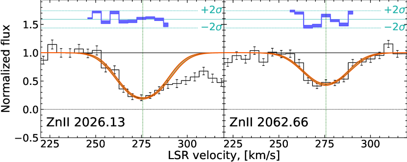
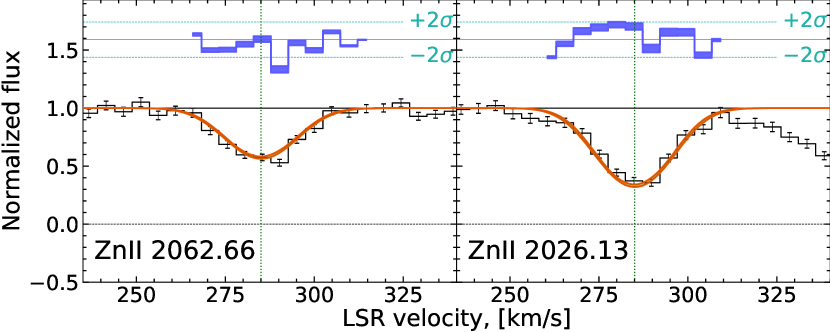
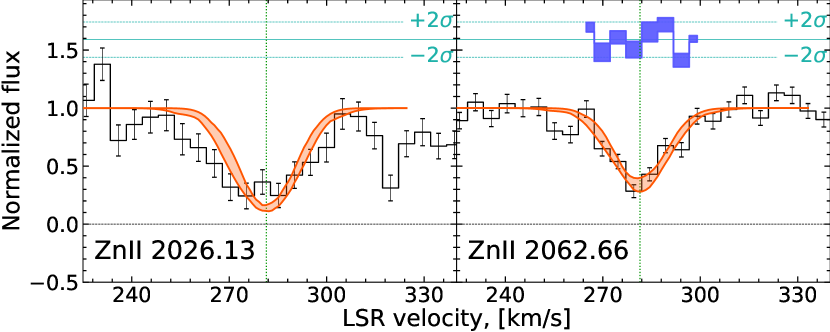
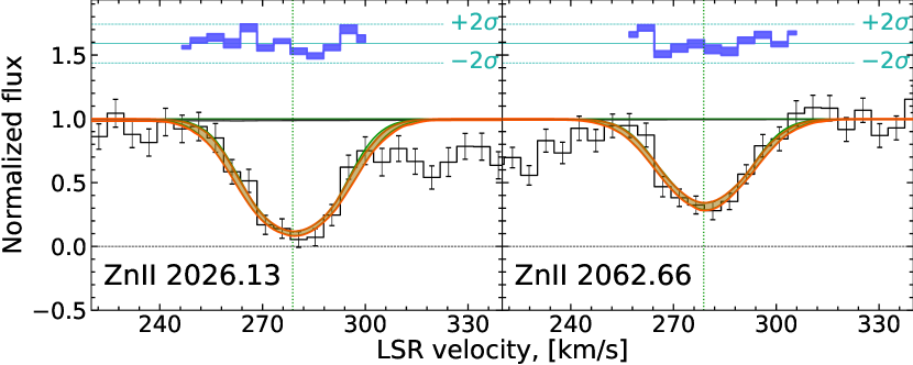
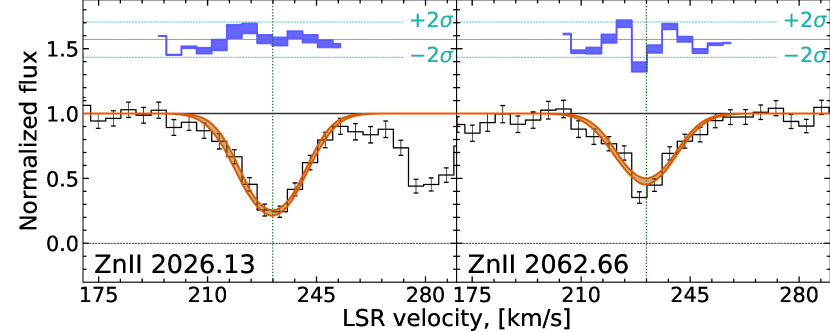
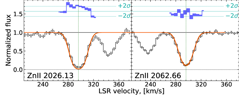
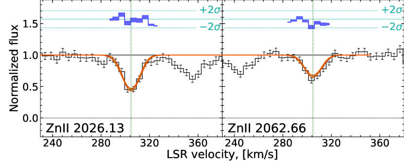
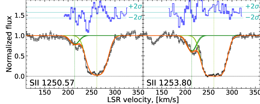
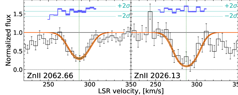
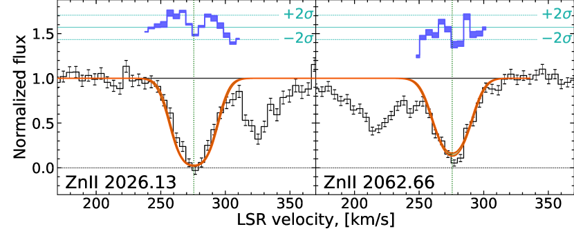
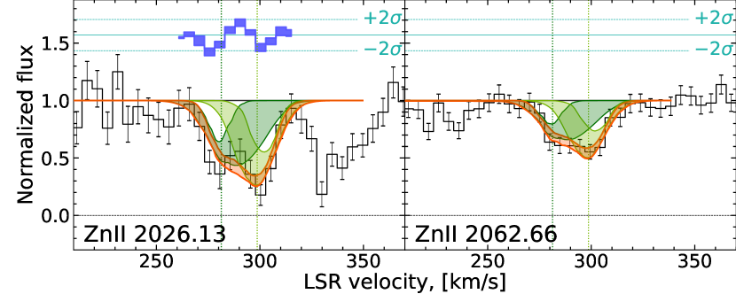
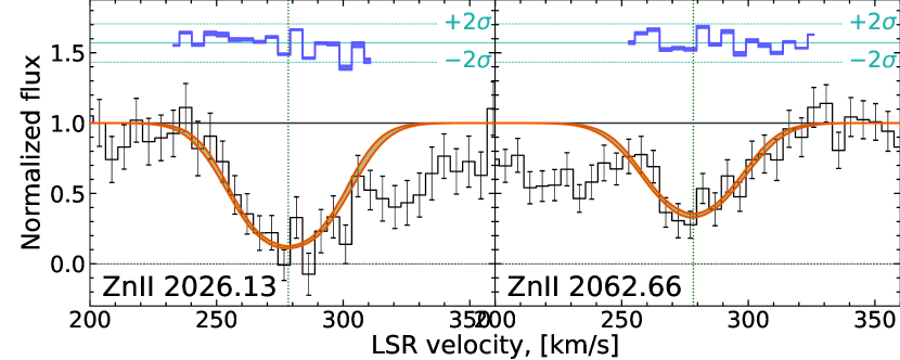
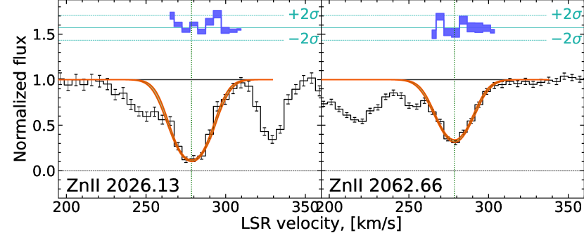
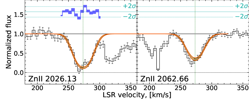
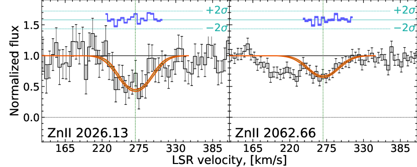
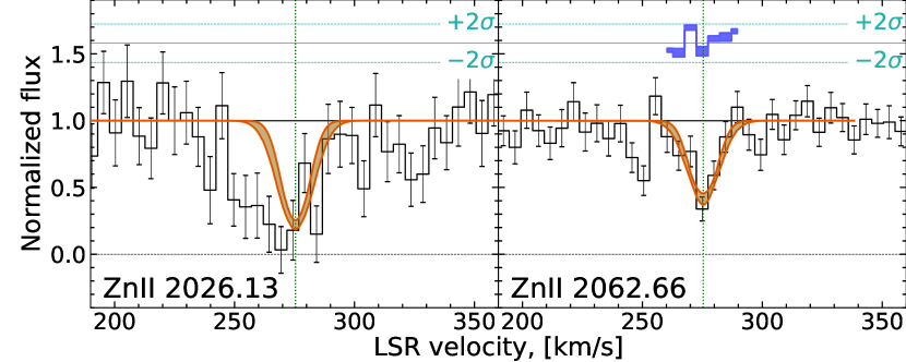
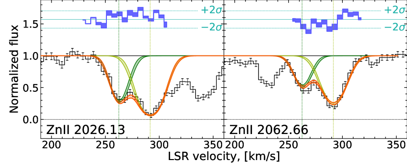
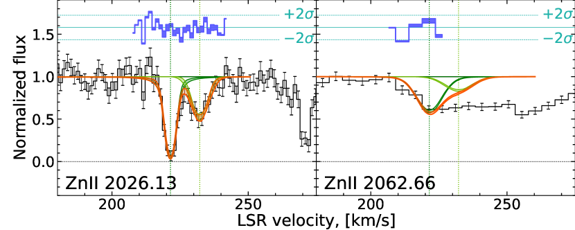
B.2 Small Magellanic Cloud

Refer to caption
Figure 92: S ii  absorption lines fit in the system towards AV 15 in the SMC. Lines are the same as in Figure 11
Refer to caption
Figure 93: Zn ii absorption lines fit in the system towards AV 26 in the SMC. Lines are the same as in Figure 11
Refer to caption
Figure 94: S ii absorption lines fit in the system towards AV 69 in the SMC. Lines are the same as in Figure 11
Refer to caption
Figure 95: Zn ii  absorption lines fit in the system towards AV 47 in the SMC. Lines are the same as in Figure 11
Refer to caption
Figure 96: S ii absorption lines fit in the system towards AV 75 in the SMC. Lines are the same as in Figure 11
Refer to caption
Figure 97: Zn ii  absorption lines fit in the system towards AV 80 in the SMC. Lines are the same as in Figure 11
Refer to caption
Figure 98: Zn ii absorption lines fit in the system towards AV 207 in the SMC. Lines are the same as in Figure 11
Refer to caption
Figure 99: Zn ii  absorption lines fit in the system towards AV 210 in the SMC. Lines are the same as in Figure 11
Refer to caption
Figure 100: Zn ii absorption lines fit in the system towards AV 216 in the SMC. Lines are the same as in Figure 11
Refer to caption
Figure 101: Zn ii  absorption lines fit in the system towards AV 216 in the SMC. Lines are the same as in Figure 11
Refer to caption
Figure 102: Zn ii absorption lines fit in the system towards AV 372 in the SMC. Lines are the same as in Figure 11
Refer to caption
Figure 103: Zn ii  absorption lines fit in the system towards AV 476 in the SMC. Lines are the same as in Figure 11
Refer to caption
Figure 104: Zn ii absorption lines fit in the system towards AV 479 in the SMC. Lines are the same as in Figure 11
Refer to caption
Figure 105: Zn ii  absorption lines fit in the system towards AV 488 in the SMC. Lines are the same as in Figure 11
Refer to caption
Figure 106: P ii absorption lines fit in the system towards AV 490 in the SMC. Lines are the same as in Figure 11
Refer to caption
Figure 107: Zn ii  absorption lines fit in the system towards Sk 191 in the SMC. Lines are the same as in Figure 11

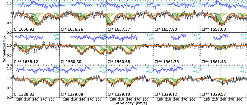
Appendix C Details on constraints of nH and $\chi$

In this section we present the constraints for each individual sightline on the number density and UV field (or CRIR) using the excitation of C i fine-structure levels and two lowest rotational levels of H2. The joint constraints are summarize in Tables 3 and 4 for the LMC and SMC, respectively

Refer to caption
Figure 108: Estimate on the number density and UV field intensity for the system towards Sk-67 2 in the LMC. Lines are the same as for Figure 4.
Refer to caption
Figure 109: Estimate on the number density and UV field intensity for the system towards Sk-67 20 in the LMC. Lines are the same as for Figure 4.
Refer to caption
Figure 110: Estimate on the number density and UV field intensity for the system towards PGMW 3070 in the LMC. Lines are the same as for Figure 4.
Refer to caption
Figure 111: Estimate on the number density and UV field intensity for the system towards LH10 3120 in the LMC. Lines are the same as for Figure 4.
Refer to caption
Figure 112: Estimate on the number density and UV field intensity for the system towards PGMW 3223 in the LMC. Lines are the same as for Figure 4.
Refer to caption
Figure 113: Estimate on the number density and UV field intensity for the system towards Sk-66 35 in the LMC. Lines are the same as for Figure 4.
Refer to caption
Figure 114: Estimate on the number density and UV field intensity for the system towards Sk-66 51 in the LMC. Lines are the same as for Figure 4.
Refer to caption
Figure 115: Estimate on the number density and UV field intensity for the system towards Sk-70 79 in the LMC. Lines are the same as for Figure 4.
Refer to caption
Figure 116: Estimate on the number density and UV field intensity for the system towards Sk-68 52 in the LMC. Lines are the same as for Figure 4.
Refer to caption
Figure 117: Estimate on the number density and UV field intensity for the system towards Sk-71 8 in the LMC. Lines are the same as for Figure 4.
Refer to caption
Figure 118: Estimate on the number density and UV field intensity for the system towards Sk-69 106 in the LMC. Lines are the same as for Figure 4.
Refer to caption
Figure 119: Estimate on the number density and UV field intensity for the system towards Sk-68 73 in the LMC. Lines are the same as for Figure 4.
Refer to caption
Figure 120: Estimate on the number density and UV field intensity for the system towards Sk-67 105 in the LMC. Lines are the same as for Figure 4.
Refer to caption
Figure 121: Estimate on the number density and UV field intensity for the system towards BI 184 in the LMC. Lines are the same as for Figure 4.
Refer to caption
Figure 122: Estimate on the number density and UV field intensity for the system towards Sk-71 45 in the LMC. Lines are the same as for Figure 4.
Refer to caption
Figure 123: Estimate on the number density and UV field intensity for the system towards Sk-71 46 in the LMC. Lines are the same as for Figure 4.
Refer to caption
Figure 124: Estimate on the number density and UV field intensity for the system towards Sk-69 191 in the LMC. Lines are the same as for Figure 4.
Refer to caption
Figure 125: Estimate on the number density and UV field intensity for the system towards BI 237 in the LMC. Lines are the same as for Figure 4.
Refer to caption
Figure 126: Estimate on the number density and UV field intensity for the system towards Sk-68 129 in the LMC. Lines are the same as for Figure 4.
Refer to caption
Figure 127: Estimate on the number density and UV field intensity for the system towards Sk-66 172 in the LMC. Lines are the same as for Figure 4.
Refer to caption
Figure 128: Estimate on the number density and UV field intensity for the system towards BI 253 in the LMC. Lines are the same as for Figure 4.
Refer to caption
Figure 129: Estimate on the number density and UV field intensity for the system towards Sk-68 135 in the LMC. Lines are the same as for Figure 4.
Refer to caption
Figure 130: Estimate on the number density and UV field intensity for the system towards Sk-69 246 in the LMC. Lines are the same as for Figure 4.
Refer to caption
Figure 131: Estimate on the number density and UV field intensity for the system towards Sk-68 140 in the LMC. Lines are the same as for Figure 4.
Refer to caption
Figure 132: Estimate on the number density and UV field intensity for the system towards Sk-71 50 in the LMC. Lines are the same as for Figure 4.
Refer to caption
Figure 133: Estimate on the number density and UV field intensity for the system towards Sk-69 279 in the LMC. Lines are the same as for Figure 4.
Refer to caption
Figure 134: Estimate on the number density and UV field intensity for the system towards Sk-68 155 in the LMC. Lines are the same as for Figure 4.
Refer to caption
Figure 135: Estimate on the number density and UV field intensity for the system towards Sk-70 115 in the LMC. Lines are the same as for Figure 4.
Refer to caption
Figure 136: Estimate on the number density and UV field intensity for the system towards AV 15 in the SMC. Lines are the same as for Figure 4.
Refer to caption
Figure 137: Estimate on the number density and UV field intensity for the system towards AV 26 in the SMC. Lines are the same as for Figure 4.
Refer to caption
Figure 138: Estimate on the number density and UV field intensity for the system towards AV 47 in the SMC. Lines are the same as for Figure 4.
Refer to caption
Figure 139: Estimate on the number density and UV field intensity for the system towards AV 69 in the SMC. Lines are the same as for Figure 4.
Refer to caption
Figure 140: Estimate on the number density and UV field intensity for the system towards AV 75 in the SMC. Lines are the same as for Figure 4.
Refer to caption
Figure 141: Estimate on the number density and UV field intensity for the system towards AV 80 in the SMC. Lines are the same as for Figure 4.
Refer to caption
Figure 142: Estimate on the number density and UV field intensity for the system towards AV 81 in the SMC. Lines are the same as for Figure 4.
Refer to caption
Figure 143: Estimate on the number density and UV field intensity for the system towards AV 207 in the SMC. Lines are the same as for Figure 4.
Refer to caption
Figure 144: Estimate on the number density and UV field intensity for the system towards AV 210 in the SMC. Lines are the same as for Figure 4.
Refer to caption
Figure 145: Estimate on the number density and UV field intensity for the system towards AV 215 in the SMC. Lines are the same as for Figure 4.
Refer to caption
Figure 146: Estimate on the number density and UV field intensity for the system towards AV 216 in the SMC. Lines are the same as for Figure 4.
Refer to caption
Figure 147: Estimate on the number density and UV field intensity for the system towards AV 266 in the SMC. Lines are the same as for Figure 4.
Refer to caption
Figure 148: Estimate on the number density and UV field intensity for the system towards AV 372 in the SMC. Lines are the same as for Figure 4.
Refer to caption
Figure 149: Estimate on the number density and UV field intensity for the system towards AV 476 in the SMC. Lines are the same as for Figure 4.
Refer to caption
Figure 150: Estimate on the number density and UV field intensity for the system towards AV 479 in the SMC. Lines are the same as for Figure 4.
Refer to caption
Figure 151: Estimate on the number density and UV field intensity for the system towards AV 488 in the SMC. Lines are the same as for Figure 4.
Refer to caption
Figure 152: Estimate on the number density and UV field intensity for the system towards AV 15 in the SMC. Lines are the same as for Figure 4.
Refer to caption
Figure 153: Estimate on the number density and UV field intensity for the system towards Sk 191 in the SMC. Lines are the same as for Figure 4.