DiffHPE: Robust, Coherent 3D Human Pose Lifting with Diffusion

Abstract

We present an innovative approach to 3D Human Pose Estimation (3D-HPE) by integrating cutting-edge diffusion models, which have revolutionized diverse fields, but are relatively unexplored in 3D-HPE. We show that diffusion models enhance the accuracy, robustness, and coherence of human pose estimations. We introduce DiffHPE, a novel strategy for harnessing diffusion models in 3D-HPE, and demonstrate its ability to refine standard supervised 3D-HPE. We also show how diffusion models lead to more robust estimations in the face of occlusions, and improve the time-coherence and the sagittal symmetry of predictions. Using the Human 3.6M dataset, we illustrate the effectiveness of our approach and its superiority over existing models, even under adverse situations where the occlusion patterns in training do not match those in inference. Our findings indicate that while standalone diffusion models provide commendable performance, their accuracy is even better in combination with supervised models, opening exciting new avenues for 3D-HPE research.

1 Introduction

3D Human Pose Estimation (3D-HPE) is rapidly evolving, with recent methods fast advancing in accuracy [8, 33]. This work joins those efforts, showcasing how integrating diffusion models into state-of-the-art models enhances not only their accuracy as previously understood, but also their robustness and coherence, as we demonstrate in our experiments.

Diffusion models, a cutting-edge generative technique, are making waves across various domains, including computer vision [23, 28, 31, 27, 19, 30], natural language processing [2, 17, 5] and time-series analysis [16, 36, 29].

The application of diffusion models to 3D-HPE (and other purely predictive tasks) remains largely unexplored, despite having shown remarkable performance in human pose forecasting, including strong robustness to occlusions [29]. In this work, we show how their ability to overcome ambiguities transposes from the latter to the former.

While a few pioneering works have shown promising performance metrics [8, 33], the understanding of the benefits of diffusion models over classical supervision — as well as key design choices — is still in its infancy. In this work, we address those concerns, providing an in-depth analysis of the effects of diffusion models on 3D-HPE.

Our contributions are threefold:

1. We propose DiffHPE, a novel strategy to use diffusion models in 3D-HPE;

2. We show that combining diffusion with supervised 3D-HPE (DiffHPE-Wrapper) outperforms each model trained separately;

3. Our extensive analyses showcase how diffusion models’ estimations display better bilateral and temporal coherence, and are more robust to occlusions, even when not perfectly trained for the latter.

2 Related work

3D Human pose estimation. Compared to 2D, 3D-HPE is much less mature, with more incipient results, especially in monocular 3D-HPE, which will be our scope. Early works in monocular 3D-HPE tackled the problem end-to-end, using deep neural networks to predict 3D keypoints directly from images [25, 22, 21, 35]. Due to persistent difficulties faced by that approach and much faster advances in 2D-HPE, the current state of the art employs a 2-step pipeline, first applying 2D-HPE, and then lifting the 2D results into 3D space.

The first methods for pose lifting used small multi-layer perceptrons [20] and nearest-neighbors matching [6].

While human pose estimation was initially tackled at the frame level, the field quickly adopted recurrent [11] and convolutional neural networks [26] to move towards video-level predictions. That allowed leveraging temporal correlations to improve accuracies. Graph convolutional networks were then proposed to exploit the keypoints’ connectivity, drastically reducing the computational complexity while improving results [42, 18, 4, 44, 12, 38].

More recently, spatial-temporal transformer architectures were proposed [32, 43], including MixSTE [41], which, arguably, is the state of the art for 3D human pose lifting among deterministic methods.

Generative human pose estimation. Lifting human pose to 3D is an inherently ambiguous task since many 3D poses may project onto the same 2D input. That led the community to investigate multi-hypothesis approaches based on generative models, such as variational autoencoders [34], normalizing flows [15, 37] and, more recently, diffusion models [8, 33].

DiffPose [8] and D3DP [33] employ a denoiser based on MixSTE, trained from scratch. D3DP [33] conditions the diffusion on the raw 2D keypoints, in a scheme that has parallels to our DiffHPE-2D (subsection 3.2). It introduces a novel hypotheses-aggregation scheme, more sophisticated than simple averaging, based on 2D reprojections, but which depends on the availability of the camera parameters.

DiffPose [8] recently set a new state of the art in 3D human pose estimation. It employs an unusual diffusion procedure based on Gaussian mixture models learned on 2D heatmaps created from the predictions of the upstream models. Besides having MixSTE as a denoiser, it employs a pre-trained MixSTE to initialize the reverse diffusion during inference — at least in the frame-level model, which is the only one released at this time.

Our proposal diverges considerably from those works. Our denoiser architecture is based on CSDI [36] and TCD [29] but introduces graph-convolutional layers that allow for good accuracy, with less computational burden than CSDI transformers. We employ a streamlined standard diffusion that forgoes the complexities of DiffPose. We use a frozen, pre-trained MixSTE as conditioning of the diffusion process, during both training and inference.

Denoising Diffusion Probabilistic Models. Denoising diffusion probabilistic models (DDPM) [9] emerged as the new state-of-the-art generative models [40], leading to impressive results in a broad range of applications such as text-to-image generation [23, 28, 31, 27], inpainting [19, 30], audio synthesis [16], time-series imputation [36] and computational chemistry [10].

They were recently applied to 3D human pose forecasting [29], showing state-of-the-art performance, including in scenarios with strong occlusions. We took great inspiration from this work, pursuing similar occlusion robustness for 3D human pose estimation.

Both our architecture and TCD [29] are based on CSDI [36], but we exchange the computation-intensive transformers of CSDI for graph-convolutional layers. We considerably extend the occlusion analysis of [29] to contemplate distribution shifts between the occlusions observed in training and those found during inference. We also include a novel analysis of the effects of diffusion on the coherence of poses.

To our knowledge, this is the first study to observe the positive impacts of diffusion — robustness to distribution shifts and improvement of symmetry and time-coherence — on 3D human poses.

3 Method

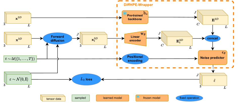
Figure 1: Training procedure of the proposed diffusion-based 2D-to-3D human pose estimation lifting. DiffHPE-Wrapper is composed of a frozen pre-trained lifting backbone $\mathrm{h}_{*}$, a linear encoding layer $\mathrm{w}_{\theta}$ for the 3D data, and noise-predicting deep neural network $\epsilon_{\theta}$. More details in subsections 3.2 and 3.4. ‘Forward diffusion’ corresponds to equation (3) and ‘concat’ to channel-wise concatenation.

3.1 Background on diffusion models

Our work builds upon DDPMs [9], a unique approach to generative modeling that has gained enormous popularity due to its extraordinary ability to represent intricate distributions, while being stable to train (when compared to GANs) and allowing for flexible architectures (when compared to normalizing flows).

DDPMs are trained to reverse a diffusion process that gradually adds Gaussian noise to the training data $\mathbf{x}_{0}$ over $T$ steps until it becomes pure noise at $\mathbf{x}_{T}$. This forward diffusion process may be formalized as sampling from a conditional distribution $\mathrm{q}$

$$\mathrm{q}(\mathbf{x}_{t}|\mathbf{x}_{t-1})=\mathcal{N}(\mathbf{x}_{t};\sqrt{1-\beta_{t}}\mathbf{x}_{t-1},\beta_{t}\mathbf{I})\,,$$ (1)

where $\mathbf{I}$ is the identity matrix and the rate at which the original data is diffused into noise is controlled by a variance scheduling given by $\beta_{1},\dots,\beta_{T}$.

Importantly, the forward process and its schedule may be reparameterized as

$$\alpha_{t}=\prod_{t=1}^{T}(1-\beta_{t}),\,$$ (2)

$$\mathrm{q}(\mathbf{x}_{t}|\mathbf{x}_{0})=\mathcal{N}(\mathbf{x}_{t};\sqrt{\alpha_{t}}\mathbf{x}_{t-1},(1-\alpha_{t})\mathbf{I}),$$ (3)

allowing to sample from each step $t$ directly. This ability is crucial for efficiently training the models.

If we knew $\mathrm{p}(\mathbf{x}_{t-1}|\mathbf{x}_{t})$, we could reverse the noise process, turning a Gaussian sample back into a sample from the data distribution. This reverse conditional distribution is arbitrarily complex, but we might approximate it via a denoising deep neural network. In particular, for small enough denoising steps, we may set

$$\mathrm{p}(\mathbf{x}_{t-1}|\mathbf{x}_{t})\approx\mathcal{N}(\mathbf{x}_{t-1};\mu_{\theta}(\mathbf{x}_{t},t),\Sigma_{t})\,,$$ (4)

where $\mu_{\theta}(\mathbf{x}_{t},t)$ is a learned deep neural network that has as input both the noisy data $\mathbf{x}_{t}$ and its step $t$ (usually position-encoded); $\Sigma_{t}$ depends on the variance schedule but is not otherwise learned.

In practice, instead of modeling $\mu_{\theta}(\mathbf{x}_{t},t)$ directly, one often prefers to, equivalently, infer the noise added to $\mathbf{x}_{t}$:

$$\mu_{\theta}(\mathbf{x}_{t},t)=k_{1,t}(\mathbf{x}_{t}-k_{2,t}\epsilon_{\theta}(\mathbf{x}_{t},t))\,,$$ (5)

where $\epsilon_{\theta}$ is the noise-predicting neural network, and $k_{.,t}$ are constants that depend on the variance schedule terms.

Conditional diffusion models, which add an extra term in the denoising process, provide a window of opportunity for purely predictive tasks:

$$\mathrm{p}(\mathbf{x}_{t-1}|\mathbf{x}_{t},c)\approx\mathcal{N}(\mathbf{x}_{t-1};\mu_{\theta}(\mathbf{x}_{t},c,t),\Sigma_{t})\,,$$ (6)

$$\mu_{\theta}(\mathbf{x}_{t},c,t)=k_{1,t}(\mathbf{x}_{t}-k_{2,t}\epsilon_{\theta}(\mathbf{x}_{t},c,t))\,,$$ (7)

where the conditioning inputs $c$ added to $\epsilon_{\theta}$ may be derived from the predictive task inputs. Conditioning allows us to leverage the power of diffusion models for 3D-HPE lifting.

3.2 Wrapping 2D-to-3D lifting with diffusion

As mentioned, the lifting approach to 3D-HPE consists in predicting the 3D positions $\mathbf{x}^{\text{3D}}$ of human keypoints from corresponding 2D positions $\mathbf{x}^{\text{2D}}$ pre-obtained by some upstream procedure. The $\mathbf{x}^{\text{3D}}$ are in the reference frame of the camera, while the $\mathbf{x}^{\text{2D}}$ lie in the pixel space of an image of height $h$ and width $w$.

We assume that 2D and 3D poses are available in a sequence of $L$ frames, each containing $J$ joints, such that $\mathbf{x}^{\text{2D}}\in(\{1,\dots,h\}\times\{1,\dots,w\})^{L\times J}\subset\mathbb{R}^{L\times J\times 2}$ and $\mathbf{x}^{\text{3D}}\in\mathbb{R}^{L\times J\times 3}$.

Traditional lifting amounts to training a deterministic, supervised regression model ${f_{\theta}:\mathbb{R}^{L\times J\times 2}\to\mathbb{R}^{L\times J\times 3}}$ on a dataset containing $N$ pairs ${\{(\mathbf{x}^{\text{2D}}_{i},\mathbf{x}^{\text{3D}}_{i}):1\leq i\leq N\}}$, estimating the conditional expectation $\mathbb{E}[\mathbf{x}^{\text{3D}}|\mathbf{x}^{\text{2D}}]$, typically using a standard mean-squared loss.

The generative flavor of lifting learns from the dataset not just the expectation, but the whole conditional distribution $\mathrm{p}(\mathbf{x}^{\text{3D}}|\mathbf{x}^{\text{2D}})$, from which candidate 3D poses can be sampled. We propose using a diffusion model, with the 3D keypoints $\mathbf{x}^{\text{3D}}$ as the target for the denoising process, and the 2D keypoints $\mathbf{x}^{\text{2D}}$ as conditioners on the process, such that the conditional DDPM formalism leads to:

$$\mathrm{p}(\mathbf{x}^{\text{3D}}_{T}|\mathbf{x}^{\text{2D}})=\mathcal{N}(\mathbf{x}^{\text{3D}}_{T};0,\mathbf{I})\,,$$ (8)

$$\mathrm{p}(\mathbf{x}^{\text{3D}}_{t-1}|\mathbf{x}^{\text{3D}}_{t},\mathbf{x}^{\text{2D}})\approx\mathcal{N}(\mathbf{x}^{\text{3D}}_{t-1};\mu_{\theta}(\mathbf{x}^{\text{3D}}_{t},\mathbf{x}^{\text{2D}},t),\Sigma_{t})\,.$$ (9)

Conditioning on the input 2D pixel coordinates. The straightforward diffusion model for lifting conditions the denoising of $\mathbf{x}^{\text{3D}}$ directly on the raw 2D data $\mathbf{x}^{\text{2D}}$, as shown in eq. (9). That is achieved in practice by feeding both $\mathbf{x}^{\text{3D}}_{t}$ and $\mathbf{x}^{\text{2D}}$ to the denoising network $\epsilon_{\theta}$ at every diffusion step $t$. We call this strategy DiffHPE-2D.

Conditioning on the features of a pre-trained model. An alternative to conditioning on the raw 2D inputs is leveraging the internal representations (feature vectors) of a pre-trained deterministic lifting model.

Suppose that ${\mathrm{f}_{*}=\mathrm{g}_{*}\circ\mathrm{h}_{*}}$ is a frozen, pre-trained lifting neural network composed of a backbone ${\mathrm{h}_{*}:\mathbb{R}^{L\times J\times 2}\to\mathbb{R}^{L\times J\times C}}$ and a linear regression head ${\mathrm{g}_{*}:\mathbb{R}^{L\times J\times C}\to\mathbb{R}^{L\times J\times 3}}$.

We could use the output of $\mathrm{h}_{*}$ instead of $\mathbf{x}^{\text{2D}}$ in eq. (9). This rich feature vector has much more information than the 3D output of $\mathrm{g}_{*}$. However, since generally $C\gg 3$, the conditioner overpowers $\mathbf{x}^{\text{3D}}_{t}$ in $\mu_{\theta}$, leading to poor performance. We mitigate that issue by also embedding $\mathbf{x}^{\text{3D}}_{t}$ into a higher-dimensional layer, such that the diffusion scheme becomes:

$$\mathbf{E}^{\text{2D}}=\mathrm{h}_{*}(\mathbf{x}^{\text{2D}})\,,\,\,\mathbf{E}^{\text{3D}}_{t}=\mathrm{w}_{\theta}(\mathbf{x}^{\text{3D}}_{t})\,,$$ (10)

$$\mathrm{p}(\mathbf{x}^{\text{3D}}_{t-1}|\mathbf{x}^{\text{3D}}_{t},\mathbf{x}^{\text{2D}})\approx\mathcal{N}(\mathbf{x}^{\text{3D}}_{t-1};\mu_{\theta}(\mathbf{E}^{\text{3D}}_{t},\mathbf{E}^{\text{2D}},t),\Sigma_{t})\,,$$ (11)

$$\mu_{\theta}(\mathbf{E}^{\text{3D}}_{t},\mathbf{E}^{\text{2D}},t)=k_{1,t}(\mathbf{x}^{\text{3D}}_{t}-k_{2,t}\epsilon_{\theta}(\mathbf{E}^{\text{3D}}_{t},\mathbf{E}^{\text{2D}},t))\,,$$ (12)

where $\mathrm{w}_{\theta}(\mathbf{x}^{\text{3D}})$ is a single trainable linear layer, and $\epsilon_{\theta}$ is the trainable noise-predicting model for the DDPM. The whole scheme is illustrated in Figures 1-2.

Since this strategy can be seen as wrapping the original lifting model $\mathrm{f}_{*}$ with the diffusion model, we call it DiffHPE-Wrapper. This diffusion model focuses on refining the lifting without the burden of working directly on the raw $\mathbf{x}^{\text{2D}}$ inputs.

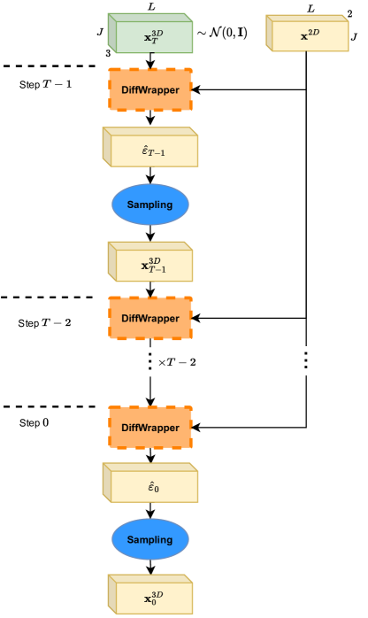
Figure 2: Human pose lifting by diffusion on 3D pose, conditioned on 2D pose. Sampling is done by following the reverse process where the noise is estimated by the trained DiffHPE model.

3.3 Noise-predictor architecture

Our noise-predicting network $\epsilon_{\theta}$ uses an architecture similar to CSDI [36], which has shown promising results for time-series imputation [36], including human pose forecasting [29]. CSDI inherits some design choices from DiffWave [16], an architecture used for audio synthesis.

Our design has 16 residual blocks, each containing two GCN layers with batch normalization, ReLU activation, and dropout, followed by a graph non-local layer [42]. We used pre-aggregated graph convolutions with decoupled self-connections [18] and 64-dimensional embeddings. The two graph-convolutional layers in each block replace the two transformer layers from CSDI [36, 29], allowing for much faster training and inference. Like in CSDI transformer layers, those two graph layers alternate between time-wise (independent convolutions for each feature, carried across time) and feature-wise (independent for each time step, carried across features). In our design, the skeleton connectivity of the human pose is always intrinsically exploited through the graph convolution connectivity. The blocks are connected through gated activation units to produce residuals, and we use the same inter-block and block-output connectivity as CSDI.

3.4 Training DiffHPE

We train DiffHPE as a standard DDPM [9]. For a given example pair ${(\mathbf{x}^{\text{2D}},\mathbf{x}^{\text{3D}})}$:

1. We sample a time-step $t\sim\mathcal{U}(\{1,\dots,T\})$;

2. We sample ${\varepsilon\in\mathbb{R}^{L\times J\times 3}}\sim\mathcal{N}(0,\mathbf{I})$ and use it to derive the noisy 3D data $\mathbf{x}^{\text{3D}}_{t}$;

3. We compute $\mathbf{E}^{\text{2D}}=\mathrm{h}_{*}(\mathbf{x}^{\text{2D}})$ and $\mathbf{E}^{\text{3D}}_{t}=\mathrm{w}_{\theta}(\mathbf{x}^{\text{3D}}_{t})$, and use them to predict the noise $\hat{\varepsilon}=\epsilon_{\theta}(\mathbf{E}^{\text{3D}}_{t},\mathbf{E}^{\text{2D}},t)$;

4. We compare $\varepsilon$ and $\hat{\varepsilon}$ with a $L_{2}$-loss, back-propagated to $\epsilon_{\theta}$ and $\mathrm{w}_{\theta}$ to learn the model parameters $\theta$.

The whole scheme is illustrated in Figure 1. Steps 1–2 correspond to eqs. (2–3), which allow for efficient sampling of training steps. We apply the steps above for all examples in the training dataset, repeating the epochs until convergence.

3.5 DiffHPE during inference

Inference follows a standard DDPM procedure (Fig. 2):

1. We sample $\mathbf{x}^{\text{3D}}_{T}\in\mathbb{R}^{L\times J\times 3}\sim\mathcal{N}(0,\mathbf{I})$;

2. We compute $\mathbf{E}^{\text{2D}}=\mathrm{h}_{*}(\mathbf{x}^{\text{2D}})$;

3. For all time steps $t$, in reverse sequence from $T$ to $1$, we:

   1. Compute $\mathbf{E}^{\text{3D}}_{t}=\mathrm{w}_{\theta}(\mathbf{x}^{\text{3D}}_{t})$, and use it to predict the noise $\hat{\varepsilon}_{t}=\epsilon_{\theta}(\mathbf{E}^{\text{3D}}_{t},\mathbf{E}^{\text{2D}},t)$;

   2. Compute $\mu_{t}$ from $\mathbf{x}^{\text{3D}}_{t}$ and $\hat{\varepsilon}_{t}$, following eq. (12);

   3. Sample $\mathbf{x}^{\text{3D}}_{t-1}\sim\mathcal{N}(\mu_{t},\Sigma_{t})$ ,

where steps 3.b and 3.c depend on non-learned constants computed from the variance schedule.

The process is obviously non-deterministic, allowing, from a single $\mathbf{x}^{\text{2D}}$ input, to sample many 3D poses $\mathbf{x}^{\text{3D}}$. We may see those samples as a parameterizable number $H$ of hypotheses for the estimated pose, which are aggregated into a final prediction.

In the literature on generative techniques, the most common “aggregation” technique is simply picking the best pose (the one closest to the ground truth), thus assessing an upper-bound performance. That is obviously unrealistic, and unfair if the comparison includes deterministic techniques. The simplest solution, which we adopt here, is to average the samples. More sophisticated strategies, such as joint-wise reprojection-based aggregation [33] could be used in situations where the intrinsic and extrinsic camera parameters are available to reproject the sampled 3D poses onto the 2D image space.

	Batch size	Learning rate	Dropout	Epochs
MixSTE[41]	$1024$	$4.0\times 10^{-5}$	$0.10$	$~{}\,500$
DiffHPE-2D	$~{}\,200$	$8.0\times 10^{-4}$	$0.03$	$1000$
DiffHPE-Wrapper	$~{}\,200$	$2.7\times 10^{-4}$	$0.27$	$1000$

Table 1: Training hyperparameters used in experiments. When possible, we used hyperparameters reported in [41] for MixSTE, while the diffusion models’ were tuned with random search.

	Diffusion	Condition	$H$	Sequence length	MPJPE   [mm]$\downarrow$	Symmetry gap [mm]$\downarrow$	Segments length std [mm]$\downarrow$
MixSTE [41]†	✗	N/A	1	27	51.8	-	-
MixSTE‡	✗	N/A	1	27	54.8	18.2	5.2
DiffHPE-2D (ours)	✓	$\mathbf{x}^{2D}$	5	27	51.8	7.0	2.1
DiffHPE-Wrapper (ours)	✓	$\mathbf{E}^{\text{2D}}$	5	27	51.2	12.4	3.2

Table 2: Comparison between MixSTE and DiffHPE. DiffHPE-2D and MixSTE$\ddagger$ act as an ablation (respectively of the conditioning on pre-trained MixSTE, and of the diffusion refinement) for DiffHPE-Wrapper. $H$ is the number of samples used to average the predicted pose. MixSTE^† is verbatim from [41], while MixSTE^‡ is reproduced from the same official code, but without the hand-tuned weighted loss and test-time augmentation, for better comparison. (Best and second best results as indicated.)

4 Experimental setting

4.1 Dataset and metrics

We use the Human 3.6M dataset [13], the most widely used dataset for 3D human pose estimation. It contains 3.6 million images of 7 actors performing 15 different actions. Both 2D and 3D ground-truth keypoints positions are available for 4 static camera viewpoints.

Following previous works [41, 8, 42], we train our models on subjects S1, S5, S6, S7, S8, and test on subjects S9 and S11.

We use the mean-per-joint-position error (MPJPE), with a 17-joint skeleton, as the main metric, following most previous works [8, 41, 42, 20]. We compute the metric under protocol #1, i.e., after translating the predicted root joint to its correct position.

4.2 Implementation details

Models. We used MixSTE [41], pre-trained on the same Human 3.6M data [13], as the frozen lifting feature extractor $\mathrm{h}_{*}$. Remark that on all experiments, the 2D input to the models, during training and test, are 2D keypoints predicted from a CPN [7] model, trained on the same data. That is important because sometimes results are reported on ground-truth 2D annotations, which leads to more optimistic results. All models were implemented in PyTorch [24].

Training. We trained the diffusion models for up to $1000$ epochs using the Adam optimizer [14] with default parameters $\beta_{1}=0.9$, $\beta_{2}=0.999$, and weight decay $=10^{-6}$. We tuned the learning rate and the dropout for all diffusion models with a random search [3] implemented in Hydra [39] and Optuna [1] (Table 1). We used a plateau learning-rate scheduler with a factor of 2 and patience of 50 epochs. We set the number of diffusion steps $T=50$ for all experiments.

Following current practice in literature and associated official code repositories that benchmark on Human 3.6M, we used the test performance both to select the hyperparameters and to pick the best checkpoint during training.

We retrained the supervised MixSTE baseline with its original parameters [41] and following the official code repository. We trained MixSTE for up to 500 epochs, significantly more than the 120 epochs reported in the paper, to ensure it had fully converged.

5 Results

5.1 Diffusion improves pre-trained lifting models

DiffHPE-Wrapper improves upon MixSTE, demonstrating its ability to refine the pre-trained model’s predictions (Table 2). In the same table, an ablation comparing both DiffHPE models showcases the compromise of using a strong baseline such as MixSTE as conditioning. On the one hand, the combined model DiffHPE-Wrapper has the best accuracy performance; on the other hand, the “purer” DiffHPE-2D model has the best indicators for pose symmetry and temporal coherence. While DiffHPE-Wrapper considerably mitigates those indicators for MixSTE, DiffHPE-2D, working ab initio, does not inherit MixSTE biases. The coherence results are analyzed in-depth in subsection 5.4, together with a detailed explanation for the metrics employed.

We report two performance values for MixSTE: one copied verbatim from the paper and another obtained by reproducing the technique in training and testing conditions identical to DiffHPE, allowing for a fairer comparison. All experiments in this table used a video length of 27 frames.

Table 3, a compilation of recent experiments from literature on longer sequences of 243 video frames, reveals the same trends for accuracy as Table 2. Unfortunately, bilateral and temporal coherence has not received much attention, preventing to evaluate trends for those metrics in the same compilation.

	Diffusion	Condition	$H$	Seq. length	MPJPE  [mm]$\downarrow$
MixSTE [41]	✗	N/A	1	243	40.9
D3DP [33]	✓	$\mathbf{x}^{2D}$	20	243	39.5
DiffPose [8]	✓	$\mathbf{E}^{\text{2D}}$	5	243	36.9

Table 3: Compilation of state-of-art human-pose lifting models. We observe the same trends as in Table 2, i.e., the diffusion models (D3DP and DiffPose) outperform the deterministic model (MixSTE), and DiffPose (which uses diffusion + MixSTE) outperforms D3DP, even with the latter using the camera parameters to aggregate 3D poses in a more sophisticated way. (Best in bold.)

5.2 Diffusion improves lifting under occlusions

Given the success of diffusion models in solving tasks such as inpainting [30, 19] and time-series imputation [36], they appear as natural candidates to address occlusions, a major challenge in human pose analysis. Indeed, they demonstrate that ability on human pose forecasting under occlusions [29]. Here, we evaluate 3D human pose lifting under the same challenging occlusion patterns proposed in [29], namely:

1. Random: any 2D keypoint in any frame may be omitted with an equal probability $p=0.2$ ;

2. Random leg and arm: any frame has a probability $p=0.4$ that all left arm and right leg keypoints are omitted;

3. Consecutive leg: a sequence of 10 consecutive frames ($\sim 40\%$ of total sequence length, picked uniformly at random) has all right leg keypoints omitted;

4. Consecutive frames: a sequence of 5 consecutive frames ($\sim 20\%$ of total sequence length, picked uniformly at random) has all keypoints completely omitted.

Omitting a keypoint corresponds to setting its value to 0.

We trained and evaluated three models (one supervised baseline MixSTE and two versions of DiffHPE-Wrapper) on all occlusion patterns, including no occlusions. Of the two DiffHPE-Wrapper models, one was conditioned on a vanilla MixSTE (trained without occlusions), and the other was conditioned on a MixSTE trained with the occlusions. The results (Table 4) show that the occlusion-trained DiffHPE beats the occlusion-trained MixSTE on all patterns. Surprisingly, the DiffHPE-Wrapper with vanilla MixSTE is competitive with the occlusion-trained MixSTE for all but the Random pattern.

	MixSTE[41]	DiffHPE-Wr.
With diffusion	✗	✓	✓
Conditioning trained w/ occ.	N/A	✗	✓
No occlusion	54.8	51.2	51.2
Random	54.5	60.3	53.2
Random leg and arm	54.4	55.2	53.0
Consecutive leg	55.1	54.1	52.6
Consecutive frames	55.8	52.2	53.5

Table 4: Impact of occlusions. Performance (MPJPE in mm) with and without diffusion under different known occlusion patterns. (Best and second best results as indicated.)

5.3 Diffusion improves robustness to occlusion-pattern misspecification

Continuing from subsection 5.2, note that training with simulated occlusions may be interpreted as a form of data augmentation. Yet, occlusions found during test time might differ from those used for training, raising the question of robustness to such domain gaps.

To investigate this question, we evaluate both occlusion-trained models (MixSTE and DiffHPE-Wrapper conditioned on it) in a cross-domain setting where training and test occlusion patterns do not necessarily match. Those results appear in Figure 3. We find that, in general, an occlusion pattern misspecification hurts the performance of both models. The performance contrast showcases interesting differences between the two models, with the diffusion model being more robust to most cases, but being particularly vulnerable to misspecification when testing on the fully Random case, suggesting the importance of structured patterns for generative modeling. On the other hand, diffusion is particularly robust when training on missing consecutive frames.

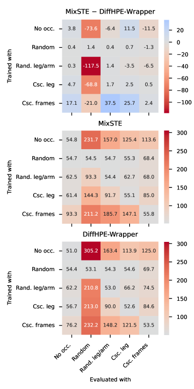
Figure 3: Impact of train/test discrepancy between occlusion patterns. Cross-domain accuracy (MPJPE in mm) with and without diffusion under different occlusion patterns. Rows correspond to occlusion patterns at training, and columns indicate occlusions at test time. The bottom two matrices show the MJPE of each method (lower is better), and the top matrix, their difference, with positive values (blue) favoring DiffHPE-Wrapper.

5.4 Diffusion improves pose coherence

The results in Table 2 already suggest that diffusion improves two aspects of the estimated poses coherence:

Symmetry. We evaluate the sagittal symmetry of predicted skeletons, i.e., segments having the same length on both sides of the body, with the average absolute difference between the length of left- and right-side segments predicted:

$$\frac{1}{KL\,S_{\text{left}}}\sum_{i=1}^{K}\sum_{l=1}^{L}\sum_{s=1}^{S_{\text{left}}}|y_{i,l,s}-y_{i,l,\tau(s)}|\,,$$ (13)

where $K$ is the number of test sequences, $L$ is the sequence length, $S_{\text{left}}$ is the number of segments on the left-side, $\tau$ maps left-side segments indices to their right-side counterpart, and $y_{i,l,s}$ is the segment’s length, given by the Euclidean distance between its two joints.

Temporal coherence. We evaluate time coherence, i.e., segment lengths not varying within a sequence, using the average of the time-wise standard deviations for each predicted segment series:

$$\frac{1}{KS}\sum_{i=1}^{K}\sum_{s=1}^{S}\sqrt{\frac{1}{L}\sum_{l=1}^{L}(y_{i,l,s}-\bar{y}_{i,s})^{2}}\,,$$ (14)

where ${\bar{y}_{i,s}=\frac{1}{L}\sum_{l=1}^{L}y_{i,l,s}}$ and $S$ is the total number of segments.

Improvements similar to Table 2 appear in Figure 4 and Figure 5, where DiffPose-Wrapper improves the coherence across all combinations of training and test occlusion-patterns (following the protocol of the previous section), including those where the accuracy results are not improved (cf. Figure 3). That latter remark is interesting, as it suggests diffusion’s ability to improve the coherence of estimations independently of “raw” accuracy gains, maybe through learning subtler hints about the data distribution.

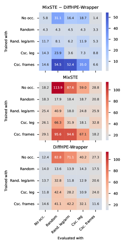
Figure 4: Impact of occlusions on sagittal symmetry of predicted poses. Average symmetry gap (in mm) with and without diffusion across different training and test occlusion patterns. The two bottom matrices show gap for the two methods (lower is better), and the top matrix, their difference, with positive values (blue) favoring DiffHPE-Wrapper.

Figure 5: Impact of occlusions on temporal consistency of segments’ length. Average time-wise standard deviation of predicted segments lengths (in mm) across different training and test occlusion patterns. The two bottom matrices show the deviation for the two methods (lower is better), and the top matrix, their difference, with positive values (blue) favoring DiffHPE-Wrapper.

6 Conclusion

We have investigated how to use diffusion models for 3D human pose lifting effectively. We show that, although diffusion models work well when used directly (DiffHPE-2D), associating them with state-of-the-art supervised models leads to even better results (DiffHPE-Wrapper). Our results demonstrate that diffusion models not only lead to more accurate predictions, but also to more time-coherent poses, which are also more compatible with the symmetry of the human body.

In future work, we plan to extend our analyses to longer sequences and find ways to mitigate the greater computational burden of diffusion, which remains its main drawback compared to classical approaches, especially during inference.

We hope this work will serve as a catalyst, showcasing the potential of diffusion models in predictive tasks and raising questions that may inspire and foster new research in this exciting area.

Acknowledgments

We are grateful to Saeed Saadatnejad for the source code of TCD [29]. This work was granted access to the HPC resources of IDRIS under the allocation 2023-AD011014073 made by GENCI.

References

- [1] Takuya Akiba, Shotaro Sano, Toshihiko Yanase, Takeru Ohta, and Masanori Koyama. Optuna: A next-generation hyperparameter optimization framework. In Proceedings of the 25rd ACM SIGKDD International Conference on Knowledge Discovery and Data Mining, 2019.
- [2] Jacob Austin, Daniel D Johnson, Jonathan Ho, Daniel Tarlow, and Rianne Van Den Berg. Structured denoising diffusion models in discrete state-spaces. Advances in Neural Information Processing Systems, 34:17981–17993, 2021.
- [3] James Bergstra and Yoshua Bengio. Random search for hyper-parameter optimization. Journal of Machine Learning Research, 13:281–305, 2012.
- [4] Yujun Cai, Liuhao Ge, Jun Liu, Jianfei Cai, Tat-Jen Cham, Junsong Yuan, and Nadia Magnenat Thalmann. Exploiting spatial-temporal relationships for 3d pose estimation via graph convolutional networks. In Proceedings of the IEEE/CVF international conference on computer vision, pages 2272–2281, 2019.
- [5] Andrew Campbell, Joe Benton, Valentin De Bortoli, Thomas Rainforth, George Deligiannidis, and Arnaud Doucet. A continuous time framework for discrete denoising models. Advances in Neural Information Processing Systems, 35:28266–28279, 2022.
- [6] Ching-Hang Chen and Deva Ramanan. 3d human pose estimation= 2d pose estimation+ matching. In Proceedings of the IEEE conference on computer vision and pattern recognition, pages 7035–7043, 2017.
- [7] Yilun Chen, Zhicheng Wang, Yuxiang Peng, Zhiqiang Zhang, Gang Yu, and Jian Sun. Cascaded pyramid network for multi-person pose estimation. In Proceedings of the IEEE conference on computer vision and pattern recognition, pages 7103–7112, 2018.
- [8] Jia Gong, Lin Geng Foo, Zhipeng Fan, Qiuhong Ke, Hossein Rahmani, and Jun Liu. DiffPose: Toward More Reliable 3D Pose Estimation. arXiv preprint arXiv:2211.16940, 2022.
- [9] Jonathan Ho, Ajay Jain, and Pieter Abbeel. Denoising diffusion probabilistic models. Advances in Neural Information Processing Systems, 33:6840–6851, 2020.
- [10] Emiel Hoogeboom, Vıctor Garcia Satorras, Clément Vignac, and Max Welling. Equivariant diffusion for molecule generation in 3d. In International Conference on Machine Learning, pages 8867–8887. PMLR, 2022.
- [11] Mir Rayat Imtiaz Hossain and James J Little. Exploiting temporal information for 3d human pose estimation. In Proceedings of the European conference on computer vision (ECCV), pages 68–84, 2018.
- [12] Wenbo Hu, Changgong Zhang, Fangneng Zhan, Lei Zhang, and Tien-Tsin Wong. Conditional directed graph convolution for 3d human pose estimation. In Proceedings of the 29th ACM International Conference on Multimedia, pages 602–611, 2021.
- [13] Catalin Ionescu, Dragos Papava, Vlad Olaru, and Cristian Sminchisescu. Human3.6M: Large Scale Datasets and Predictive Methods for 3D Human Sensing in Natural Environments. IEEE Transactions on Pattern Analysis and Machine Intelligence, 36(7):1325–1339, July 2014.
- [14] Diederik P Kingma and Jimmy Ba. Adam: A method for stochastic optimization. arXiv preprint arXiv:1412.6980, 2014.
- [15] Nikos Kolotouros, Georgios Pavlakos, Dinesh Jayaraman, and Kostas Daniilidis. Probabilistic modeling for human mesh recovery. In Proceedings of the IEEE/CVF international conference on computer vision, pages 11605–11614, 2021.
- [16] Zhifeng Kong, Wei Ping, Jiaji Huang, Kexin Zhao, and Bryan Catanzaro. Diffwave: A versatile diffusion model for audio synthesis. arXiv preprint arXiv:2009.09761, 2020.
- [17] Xiang Li, John Thickstun, Ishaan Gulrajani, Percy S Liang, and Tatsunori B Hashimoto. Diffusion-lm improves controllable text generation. Advances in Neural Information Processing Systems, 35:4328–4343, 2022.
- [18] Kenkun Liu, Rongqi Ding, Zhiming Zou, Le Wang, and Wei Tang. A comprehensive study of weight sharing in graph networks for 3d human pose estimation. In European Conference on Computer Vision, pages 318–334. Springer, 2020.
- [19] Andreas Lugmayr, Martin Danelljan, Andres Romero, Fisher Yu, Radu Timofte, and Luc Van Gool. Repaint: Inpainting using denoising diffusion probabilistic models. In Proceedings of the IEEE/CVF Conference on Computer Vision and Pattern Recognition, pages 11461–11471, 2022.
- [20] Julieta Martinez, Rayat Hossain, Javier Romero, and James J Little. A simple yet effective baseline for 3d human pose estimation. In Proceedings of the IEEE international conference on computer vision, pages 2640–2649, 2017.
- [21] Dushyant Mehta, Srinath Sridhar, Oleksandr Sotnychenko, Helge Rhodin, Mohammad Shafiei, Hans-Peter Seidel, Weipeng Xu, Dan Casas, and Christian Theobalt. Vnect: Real-time 3d human pose estimation with a single rgb camera. Acm transactions on graphics (tog), 36(4):1–14, 2017.
- [22] Francesc Moreno-Noguer. 3d human pose estimation from a single image via distance matrix regression. In Proceedings of the IEEE conference on computer vision and pattern recognition, pages 2823–2832, 2017.
- [23] Alex Nichol, Prafulla Dhariwal, Aditya Ramesh, Pranav Shyam, Pamela Mishkin, Bob McGrew, Ilya Sutskever, and Mark Chen. Glide: Towards photorealistic image generation and editing with text-guided diffusion models. arXiv preprint arXiv:2112.10741, 2021.
- [24] Adam Paszke, Sam Gross, Francisco Massa, Adam Lerer, James Bradbury, Gregory Chanan, Trevor Killeen, Zeming Lin, Natalia Gimelshein, Luca Antiga, et al. Pytorch: An imperative style, high-performance deep learning library. Advances in neural information processing systems, 32, 2019.
- [25] Georgios Pavlakos, Xiaowei Zhou, Konstantinos G Derpanis, and Kostas Daniilidis. Coarse-to-fine volumetric prediction for single-image 3D human pose. In Proceedings of the IEEE conference on computer vision and pattern recognition, pages 7025–7034, 2017.
- [26] Dario Pavllo, Christoph Feichtenhofer, David Grangier, and Michael Auli. 3d human pose estimation in video with temporal convolutions and semi-supervised training. In Proceedings of the IEEE/CVF Conference on Computer Vision and Pattern Recognition, pages 7753–7762, 2019.
- [27] Aditya Ramesh, Prafulla Dhariwal, Alex Nichol, Casey Chu, and Mark Chen. Hierarchical text-conditional image generation with clip latents. arXiv preprint arXiv:2204.06125, 2022.
- [28] Robin Rombach, Andreas Blattmann, Dominik Lorenz, Patrick Esser, and Björn Ommer. High-resolution image synthesis with latent diffusion models. In Proceedings of the IEEE/CVF conference on computer vision and pattern recognition, pages 10684–10695, 2022.
- [29] Saeed Saadatnejad, Ali Rasekh, Mohammadreza Mofayezi, Yasamin Medghalchi, Sara Rajabzadeh, Taylor Mordan, and Alexandre Alahi. A generic diffusion-based approach for 3D human pose prediction in the wild, Oct. 2022.
- [30] Chitwan Saharia, William Chan, Huiwen Chang, Chris Lee, Jonathan Ho, Tim Salimans, David Fleet, and Mohammad Norouzi. Palette: Image-to-image diffusion models. In ACM SIGGRAPH 2022 Conference Proceedings, pages 1–10, 2022.
- [31] Chitwan Saharia, William Chan, Saurabh Saxena, Lala Li, Jay Whang, Emily L Denton, Kamyar Ghasemipour, Raphael Gontijo Lopes, Burcu Karagol Ayan, Tim Salimans, et al. Photorealistic text-to-image diffusion models with deep language understanding. Advances in Neural Information Processing Systems, 35:36479–36494, 2022.
- [32] Wenkang Shan, Zhenhua Liu, Xinfeng Zhang, Shanshe Wang, Siwei Ma, and Wen Gao. P-STMO: Pre-Trained Spatial Temporal Many-to-One Model for 3D Human Pose Estimation, July 2022.
- [33] Wenkang Shan, Zhenhua Liu, Xinfeng Zhang, Zhao Wang, Kai Han, Shanshe Wang, Siwei Ma, and Wen Gao. Diffusion-based 3d human pose estimation with multi-hypothesis aggregation. arXiv preprint arXiv:2303.11579, 2023.
- [34] Saurabh Sharma, Pavan Teja Varigonda, Prashast Bindal, Abhishek Sharma, and Arjun Jain. Monocular 3d human pose estimation by generation and ordinal ranking. In Proceedings of the IEEE/CVF international conference on computer vision, pages 2325–2334, 2019.
- [35] Xiao Sun, Jiaxiang Shang, Shuang Liang, and Yichen Wei. Compositional human pose regression. In Proceedings of the IEEE International Conference on Computer Vision, pages 2602–2611, 2017.
- [36] Yusuke Tashiro, Jiaming Song, Yang Song, and Stefano Ermon. CSDI: Conditional score-based diffusion models for probabilistic time series imputation. Advances in Neural Information Processing Systems, 34:24804–24816, 2021.
- [37] Tom Wehrbein, Marco Rudolph, Bodo Rosenhahn, and Bastian Wandt. Probabilistic monocular 3d human pose estimation with normalizing flows. In Proceedings of the IEEE/CVF international conference on computer vision, pages 11199–11208, 2021.
- [38] Tianhan Xu and Wataru Takano. Graph stacked hourglass networks for 3d human pose estimation. In Proceedings of the IEEE/CVF conference on computer vision and pattern recognition, pages 16105–16114, 2021.
- [39] Omry Yadan. Hydra - a framework for elegantly configuring complex applications. Github, 2019.
- [40] Ling Yang, Zhilong Zhang, Yang Song, Shenda Hong, Runsheng Xu, Yue Zhao, Yingxia Shao, Wentao Zhang, Bin Cui, and Ming-Hsuan Yang. Diffusion models: A comprehensive survey of methods and applications. arXiv preprint arXiv:2209.00796, 2022.
- [41] Jinlu Zhang, Zhigang Tu, Jianyu Yang, Yujin Chen, and Junsong Yuan. Mixste: Seq2seq mixed spatio-temporal encoder for 3d human pose estimation in video. In Proceedings of the IEEE/CVF Conference on Computer Vision and Pattern Recognition, pages 13232–13242, 2022.
- [42] Long Zhao, Xi Peng, Yu Tian, Mubbasir Kapadia, and Dimitris N Metaxas. Semantic graph convolutional networks for 3d human pose regression. In Proceedings of the IEEE/CVF conference on computer vision and pattern recognition, pages 3425–3435, 2019.
- [43] Ce Zheng, Sijie Zhu, Matias Mendieta, Taojiannan Yang, Chen Chen, and Zhengming Ding. 3D Human Pose Estimation with Spatial and Temporal Transformers. In 2021 IEEE/CVF International Conference on Computer Vision (ICCV), pages 11636–11645, Montreal, QC, Canada, Oct. 2021. IEEE.
- [44] Zhiming Zou and Wei Tang. Modulated graph convolutional network for 3d human pose estimation. In Proceedings of the IEEE/CVF International Conference on Computer Vision, pages 11477–11487, 2021.