Object Size-Driven Design of Convolutional Neural Networks: Virtual Axle Detection based on Raw Data

Abstract

Rising maintenance costs of ageing infrastructure necessitate innovative monitoring techniques. This paper presents a new approach for detecting axles, enabling real-time application of Bridge Weigh-In-Motion (BWIM) systems without dedicated axle detectors. The proposed Virtual Axle Detector with Enhanced Receptive Field (VADER) is independent of bridge type and sensor placement while only using raw acceleration data as input. By using raw data instead of spectograms as input, the receptive field can be enhanced without increasing the number of parameters. We also introduce a novel receptive field (RF) rule for an object-size driven design of Convolutional Neural Network (CNN) architectures. We were able to show, that the RF rule has the potential to bridge the gap between physical boundary conditions and deep learning model development. Based on the RF rule, our results suggest that models using raw data could achieve better performance than those using spectrograms, offering a compelling reason to consider raw data as input. The proposed VADER achieves to detect 99.9 % of axles with a spatial error of 4.13 cm using only acceleration measurements, while cutting computational and memory costs by 99 % compared to the state-of-the-art using spectograms.

[label0]organization=Institute of Structural Mechanics and Design, Department of Civil and Environmental Engineering, Technical University of Darmstadt,addressline=Franziska-Braun-Str. 3, city=Darmstadt, postcode=64287, state=Hesse, country=Germany

1 Introduction

As infrastructure ages, novel methods are imperative for efficient monitoring. Precise knowledge of the actual stress and loads on infrastructure enables more accurate determination of remaining service life, identification of overloaded vehicles, and more efficient planning for new constructions. Measuring loads directly is very difficult in many cases. Instead, loads can be reconstructed via the structural response [1, 2, 3, 4, 5, 6]. Based on this, Weigh-In-Motion (WIM) systems are used to reconstruct the axle loads of trains or cars. WIM systems have the advantage of being able to determine the axle loads in the regular traffic flow. Conventional WIM systems necessitate installation directly into roadways or tracks, often requiring traffic disruption. Conventional WIM systems are therefore expensive and hardly suitable for a nationwide investigation of axle loads. In contrast, Bridge WIM systems (BWIM) are positioned beneath bridge structures, facilitating reuse and repositioning for multiple BWIM measurements [7, 8, 9, 10]. Thus, the installation of a BWIM system is less expensive and can be used for a multitude of time-limited investigations.

For large-scale investigations of axle loads, BWIM systems are therefore hardly dispensable. However, effective utilisation of BWIM systems typically demands knowledge of the axle positions [10, 11, 12]. For this purpose, additional sensors currently need to be installed at specific locations (facing the roadway, on the cross girders, or near the supports) that depend on the bridge structure [13, 14, 15, 16]. Only in the case of thin slab bridges can BWIM strain sensors be reliably used for axle detection [17]. Tan et al. [18] has proposed a BWIM system that works without axle detectors, but this system is dependent on strain measurements and only works for one vehicle at a time on the bridge. However, for a large scale application of BWIM measurements, a method for axle detection and localisation that is independent of bridge type, measured physical quantities and sensor position would be of great benefit, effectively reducing cost and risk. Therefore, our study aims at an axle detection method using existing sensors of arbitrary BWIM systems. To determine the axle positions, axles are usually detected at at least two locations. With the distance between the locations and the difference in time, the axle position can then be interpolated or extrapolated in time.

The term Sound Event Detection (SED) is predominantly used in the literature for the detection of events in time series [19, 20, 21, 22]. One of the tasks of SED is for example speech recognition. Here, events refer to words and audible sound is used as input. However, this methodology can also be applied to other vibration signals as input (such as accelerations in bridges) to find events like a train axle passing a bridge. For SED problems, time series are typically analysed in the form of 2D spectrograms using Convolutional Neural Networks (CNNs) [23, 24] or, more recently, Transformers [25], despite the competitive performance of 1D CNNs [26]. Consequently, research often concentrates on identifying the most suitable spectrogram type [27, 28]. Notably, in conventional tasks like speech recognition and acoustic scene classification, log mel spectrograms dominate [20, 29, 25], despite some studies showing better or comparable outcomes using raw data [27, 30, 31, 32]. In the context of axle localisation, Continuous Wavelet Transformations (CWTs) have demonstrated suitability as features for axle detection [33, 34, 35, 12, 36, 37]. Given that CWTs even compete well in speech recognition [27] and log mel spectrograms were tailored for human auditory perception, CWTs were adopted in our earlier work for axle detection [37]. However, it is unclear whether CWTs are actually necessary, whether raw measurement data is sufficient as model input, and how this affects the model’s performance.

In addition, there are only a few guidelines for the hyperparameters and architectures for the development of neural networks and these usually refer to empirical values [38]. In order to adapt models for new problems faster and more reliably, we propose in this study a receptive field rule based on object sizes and validate it on the virtual axle detector. The object size in this case refers to the minimum natural frequency of a bridge, but the basic principle should also be transferable to other domains such as sound or images.

In this study, we propose a novel approach that enables real-time detection and localisation of axles using arbitrarily placed sensors. For each sensor, the axles are localised at the nearest point of the tracks to the sensor (perpendicular to the direction of travel). The position can also be determined multi-dimensionally using several sensors, making the concept presented here relevant for car bridges as well. Consequently, BWIM systems can now conduct real-time axle detection without the need for additional sensors. The concept is validated on a single track railway bridge. This means that in this study there is only one train at a time on the bridge on a ballasted track. To make it transferable to car bridges, the axles were always considered individually and not as part of a vehicle. The proposed concept determines the longitudinal position of axles using sensors distributed longitudinally. A transversal distribution of additional sensors could therefore determine the position of the axles in two directions. Thus, the approach is theoretically also applicable for multi-lane car bridges. To validate our approach, we adapted the VAD model [37] to handle raw measurement data and performed several tests on the dataset from Lorenzen et al. [39].

2 Methodology

In this section, we outline the methodology used for the Virtual Axle Detector with Enhanced Receptive field (VADER) and the investigations on the influence of the input data in the form of spectograms or raw measurement data. The used data set [39] is briefly summarized. Finally, the training parameters and evaluation metrics are described.

2.1 Data Acquisition

The dataset from Lorenzen et al. [39] was acquired on a single-span steel trough railway bridge situated on a long-distance traffic line in Germany (fig. 1). This bridge is 18.4 meters long with a free span of 16.4 meters and a natural frequency of about 6.9 Hz for the first bending mode. The natural frequency is variable with a non-linear dependence on the load due to the ballast [40]. Measurement data from ten seismic uniaxial accelerometers with a sampling rate of 600 Hz installed along the bridge are used as features.

Utilizing a supervised learning approach, our model requires labels as the ground truth from which to learn. For the creation of the labels, four rosette strain gauges directly installed on the rails (fig. 1) were used to ensure that the accuracy of the assumed ground truth is sufficient to accurately evaluate the performance of the model. The rosette strain gauges were used to determine the axle positions and velocities of the passing trains. This was then used to determine the points in time at which the axles were closest to the individual acceleration sensors (perpendicular to the direction of travel). By using this as a label, the model is trained to use the acceleration sensors as a virtual light barrier that is triggered when a train axle is crossed [37]. The label vector contains ones at the time points when a train axle is positioned above the respective sensor, and the rest are zeros (fig. 2). Therefore, the sum of the label vector yields the number of axles of the corresponding train. The model then only receives the acceleration signals of a single sensor at a time and predicts the times at which an axle is located above this sensor. From a number of two acceleration sensors, the axle distances and velocities can thus also be determined. Due to the sampling rate, an inaccuracy of 6-38 cm is assumed for the label creation, depending on the train’s velocity and the sensor’s position. The dataset consist out of 3,745 train passages with one label vector per sensor. For more detailed information about the dataset and the measurement campaign, please refer to the paper by Lorenzen et al. [37].

To ensure that strain gauge measurements are not necessary for the application, two scenarios for labeling are investigated in this study: a) existing data from a failed axle detector and b) trains with a differential global positioning system (DGPS).

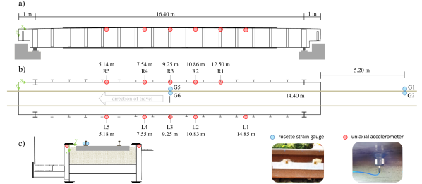
Figure 1: Bridge and sensor setup a) side view b) top view with sensor labels, accelerometers $x$-ordinate and strain gauge distances c) cross section. [37]

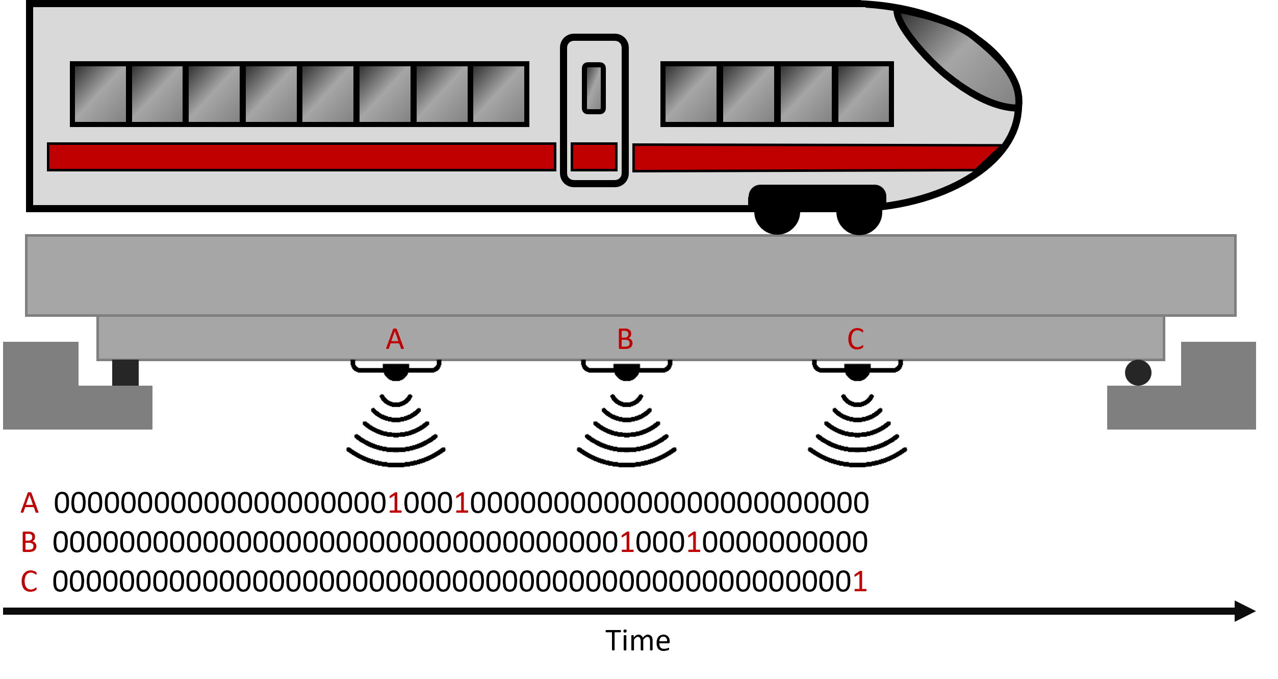
Figure 2: The labels represent the moment when a train axle is located over the respective sensor. Here, as an example, potential label vectors are shown for three fictitious sensors and a train up to the time shown.

2.2 Data Transformation

To investigate the influence of data representation, two cases are considered: a) spectograms and b) raw measurement data. The spectograms are the same as proposed by Lorenzen et al. [37] with three mother wavelets and two sets of 16 frequencies per mother wavelet as input per crossing and sensor (tab. 1). This results in an input tensor of $16\times 6\times n_{\mathrm{s}}$ with $n_{\mathrm{s}}$ being the number of samples in the acceleration signal of a sensor. The raw measurement data was used unchanged as input and not even scaled or normalized.

	Scale Limit
Wavelet	Lower	Upper
First Order Complex Gaussian Derivative	1	8
	8	50
First Order Gaussian Derivative	0.6	6.5
	6.5	35
Default Frequency B-Spline from Lee et al. [41]	1.5	10
	10	40

Table 1: The transformation settings used per passage and per signal. Derived from Lorenzen et al. [37].

2.3 Data Split

The training and validation sets were implemented using a five-fold cross-validation approach with a holdout test set. Initially, one-sixth of the data was separated for the test set. The remaining data was divided into five folds. During training, a different fold was used as the validation set in each iteration, while the other four folds were used for training. Training concluded based on the validation set results, and the model was consistently tested on the same test set. This process allowed the model to be evaluated five times using the same data, providing a more accurate estimation of its generalization capability [38].

To further investigate the applicability of the proposed concept, the dataset was split into training and testing based on the number of train axles in two different ways. In the first split, the model is intended to function as a surrogate for a malfunctioning axle detector. For this purpose, the data set was split for all folds and the test set in a stratified fashion (fig. 3(a)), resulting in 3,110 passages with 112,038 individual axles for training and 623 passages with 22,472 individual axles for testing.

In the second split, the model was provided only with axle positions from trains of a single type. This simulates a scenario in which only one train type is equipped with a differential global positioning system (DGPS), but the axles of all other train types still need to be recognized. This allows the robustness of the method and the overfitting of the model to be examined. Since the exact construction series of the trains for determining the train types are not known, the train length in axles was used as a simplified criterion instead. Trains with the most frequent axle count were used for the five-fold cross-validation sets, while all other train lengths were included in the test set (fig. 3(b)). This results in 1,916 passages with 61,312 individual axles for training and 1,817 passages with 73,198 individual axles for testing.

With the stratified splits, training is done with about 5/6 of the data and testing with 1/6 of the data, whereas the splits in the DGPS set for training and testing are about the same size. Thus, in the case of DGPS splits, in addition to having significantly less data available for training, these data are also not representative of the test data and therefore not for all trains. It should be noted that with non-representative data sets, inadequate results are usually to be expected [38]. Thus, the DPGS splits are suitable for testing the models under particularly difficult conditions.

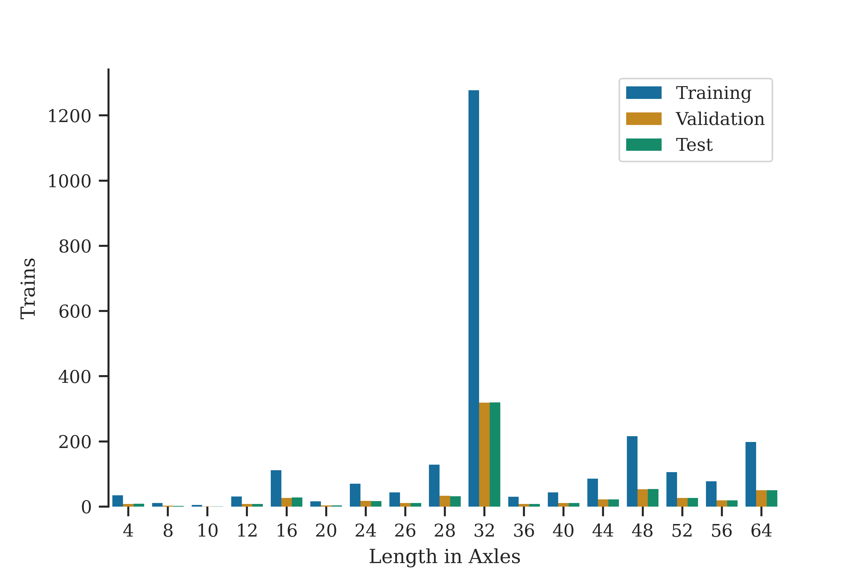
(a) Stratified data splits

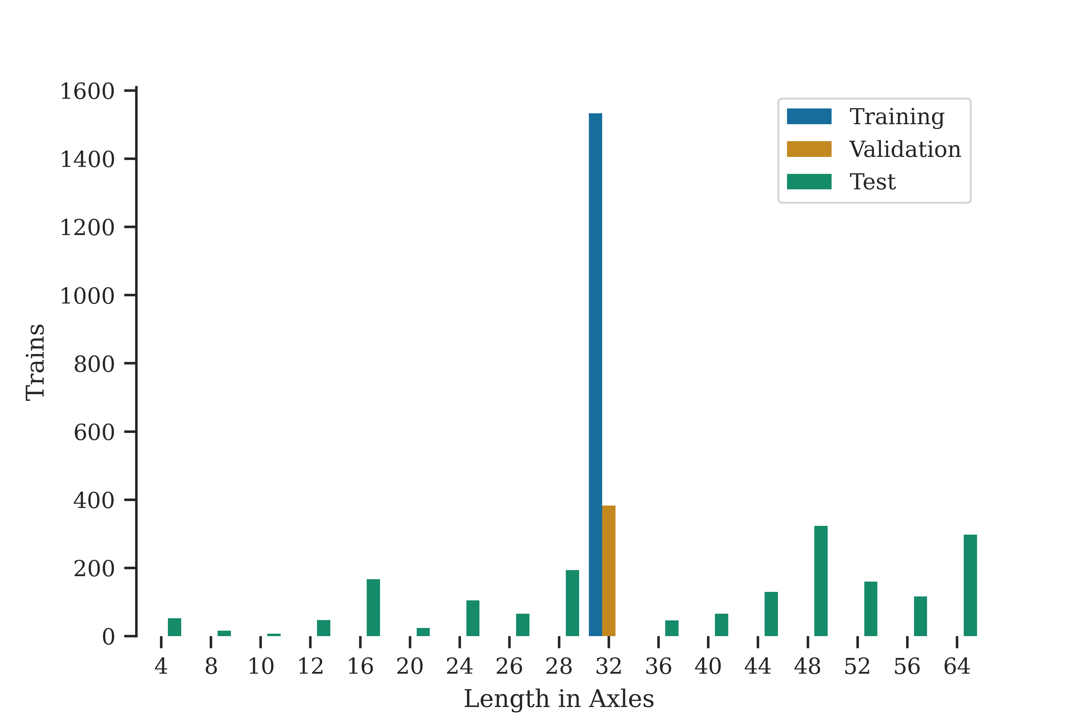
(b) DGPS data splits

Figure 3: Train lengths defined by number of axles in both splits for the first combination of folds of a five-fold cross-validation.

2.4 Model Definition

The VADER model is implemented as a fully convolutional neural network (FCN) [42] to handle inputs of arbitrary lengths. This property is particularly advantageous for the detection of train axles, as the crossing time varies significantly based on the train’s speed and the number of axles.

The U-Net concept [43] was chosen for the model architecture, originally developed for semantic segmentation of images, but also adaptable for segmenting time series data. The fundamental concept of the U-Net architecture is the encoder and decoder path. Even though new architectures have been developed, the U-Net architecture is still frequently used as backbone [44, 45, 46]. In order to investigate the effects of the hyperparameters kernel size, max pooling size and pooling steps, no other model architectures are considered in this study. In the encoder path, the resolution is progressively reduced and information is compressed, while in the decoder path, the resolution is increased back to the original dimensions (fig. 4(a)). The encoder path aims to capture details at various resolutions, while the decoder path integrates these details into the appropriate context. The intermediate results from the encoder and decoder paths at the same resolution are combined through skip connections.

Our implementation of the U-Net comprises of a well established combination [38] of convolution blocks (CBs), residual blocks (RBs) originally proposed by He et al. [47], max pooling layers, concatenate layers, and transposed convolution layers (fig. 4). A CB always consists of a convolution layer with Rectified Linear Unit (ReLU) activation and a group normalisation layer [48]. The first group normalisation layer has a single group (making it nearly identical to Layer Normalisation [48]) and remaining group norm layers have 16 channels per group. As a result, the measurement data is first normalised individually (as 1 channel per sensor) in the first group normalisation layer and the remaining CNN feature maps are normalised with the optimum group size according to Wu and He [48]. Group normalisation was shown to be less sensitive to other hyperparameters like batch size and was therefore chosen to effectively reduce the hyperparameter space. The RBs were implemented similarly to the 50-layer or larger variants of the ResNet [47]. The final layer in both models is a convolution layer with only one filter and sigmoid activation.

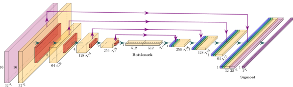
(a) VADER with spectograms (VADERspec) as input and 4 pooling steps. Derived from Lorenzen et al. [37].

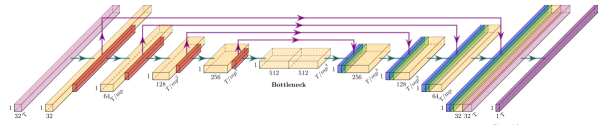
(b) VADER with raw data (VADERraw) as input and 4 pooling steps.

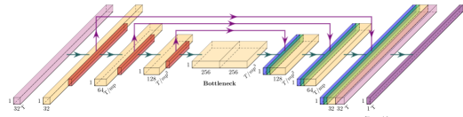
(c) VADER with raw data (VADERraw) as input and 3 pooling steps.

Figure 4: Model definition with colored boxes corresponding to the following layers: CB (light purple), RB (yellow), max pooling (red), concatenate (green), transposed convolution (blue) and reshaping skip connection (purple arrow). Dimension of the feature maps at the corresponding boxes with $T$ for samples and $mp$ for max pooling size at the bottom right, feature maps at the bottom and frequencies at the left.

VADER with spectograms (VADERspec) as input (fig. 4(a)) uses the default kernel size of $3\times 3$ and the default pooling size of 2 for 2D inputs [38]. This halves the temporal resolution with each pooling step. In the bottleneck layers, the temporal resolution is reduced by a factor of 16, giving the model a receptive field of $16\times 3=48$ with a kernel size of 3. Thus, the model can analyse a time frame of at least 48 samples at once.

Since VADER with raw data (VADERraw) as input (fig. 4(b)) processes only 1D data, the same number of parameters are required for a kernel size of $9\times 1$ as for the kernel size of $3\times 3$ in the VADERspec model. As the kernel size is larger, the pooling size can also be increased. In order to determine the optimal pooling size, kernel size and amount of pooling steps we propose the receptive field (RF) rule: To achieve good results with a CNN, the largest effective receptive field must be at least as large as the largest object of interest. The effective receptive field refers to the number of samples that the kernel could see at the original resolution/sampling rate. After a max pooling layer of size two, the effective receptive field would therefore double with the same kernel size. In our case, the RF rule can be used to calculate the required size of the largest receptive field to capture the lowest frequency of interest:

$$y\geq\frac{f_{\mathrm{s}}}{f_{\mathrm{l}}},$$ (1)

with $f_{\mathrm{s}}$ as sample frequency, $f_{\mathrm{l}}$ as lowest frequency of interest and y as the necessary size of the models largest receptive field in samples. Hence, to cover signals of, e.g., 1 Hz at a sampling rate of 600 Hz, the receptive field must span at least 600 samples (eq. 1).

The bridge has a natural frequency of up to 6.9 Hz (depending on the amplitude), and to distinguish the contribution of the bridge from the axle loads’ structural response, a receptive field of at least $\frac{600~{}Hz}{6.9~{}Hz}\approx 87$ samples would be necessary. Taking into account that the resonance frequency decreases to about 5.6 Hz for big amplitudes [49], a minimum receptive field of $\frac{600~{}Hz}{5~{}Hz}=120$ samples ensures that more than the largest object size is captured.

Much like CNNs, the wavelet convolves over the samples, effectively encoding frequency information into individual sample values through the CWT transformation. Depending on the wavelet and the scale, different frequencies are filtered. With the parameters used, information on frequencies up to approximately 3.4 Hz is therefore encoded in individual samples. Therefore, the CWT transformation can effectively increase the receptive field for VADERspec to $\frac{600~{}Hz}{3.4~{}Hz}\approx 176$ samples.

With a pooling size of 3, a kernel size of 9 and 4 pooling steps, VADERraw would result in a maximum receptive field of $3^{4}\times 9=729$ samples. Therefore, in this case the actual receptive field of VADERraw is over 15 times larger (729 vs. 48) and the effective receptive field is over 4 times larger (729 vs. 176) than that of VADERspec, while using the same number of parameters. As bigger a RF does not always lead to better results, two amounts of pooling steps, eight different kernel sizes and four different max pooling sizes were examined as a hyperparameter study (fig. 5).

Depending on the hyperparameter combinations, there are large differences in the maximum repective field size of the respective model (fig. 5). With a required minimum receptive field size of 87-120 samples (depending on whether the natural frequency is considered constant or not), a small proportion of the models are expected to perform significantly worse (dark purple in Fig. 5). From a RF size above $\frac{600~{}Hz}{1~{}Hz}\approx 600$ samples there is expected to be no more improvement in the results (light orange in Fig. 5). There are no objects with frequencies lower than 1 Hz that the model should be able to detect. An RF that can capture frequencies of 1 Hz already allows to capture several bridge oscillation periods in one RF. Beyond that, the risk increases that entire trains and thus axle configurations are learned by the model. This would therefore increase the probability of overfitting and reduce the generalisation capability.

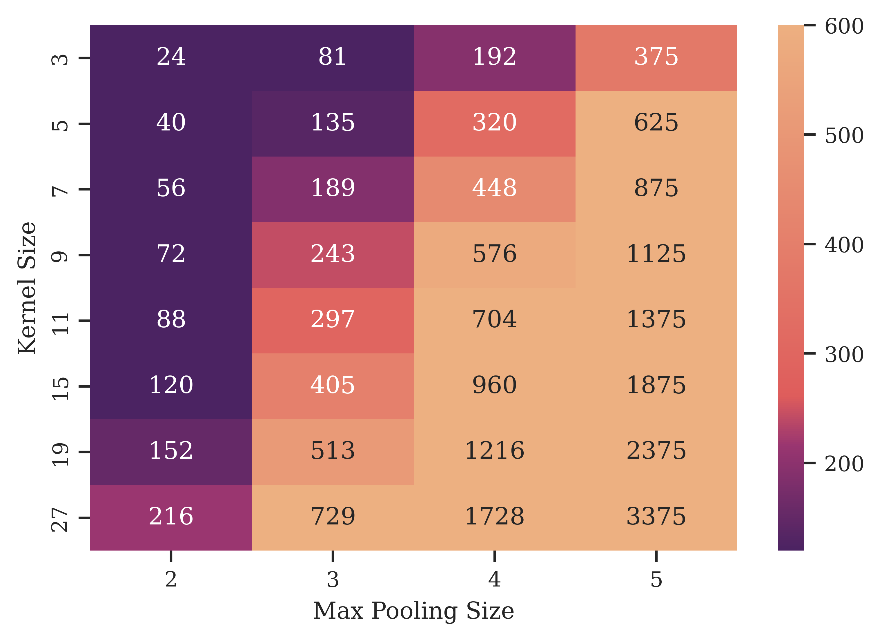
(a) Resulting maximum receptive fields for VADERraw with 3 pooling steps.

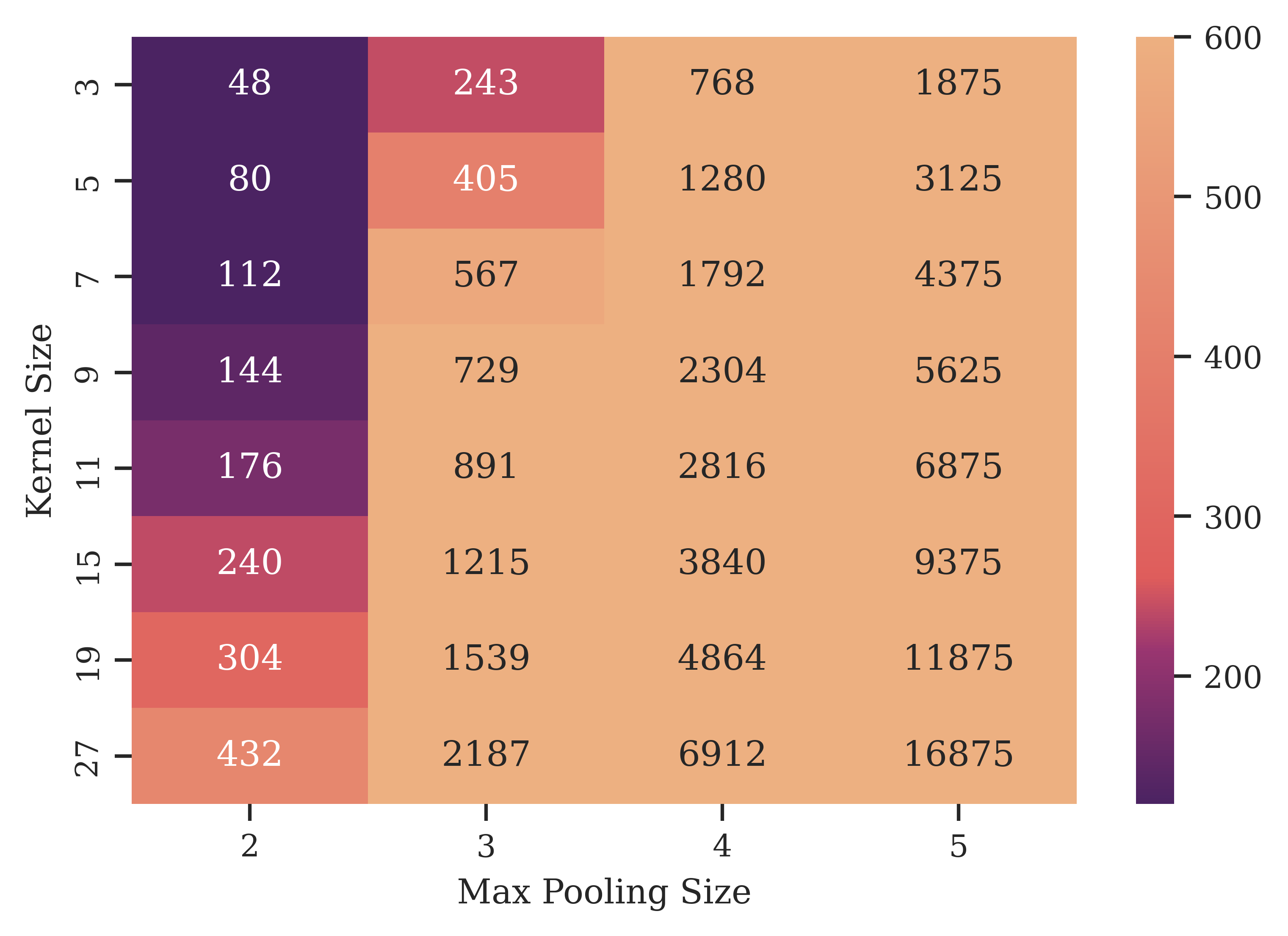
(b) Resulting maximum receptive fields for VADERraw with 4 pooling steps.

Figure 5: Maximum receptive fields as a function of kernel size, max pooling size and pooling steps for all used combinations of the hyperparameter study.

The TensorFlow library [50] was used for implementation of the models and PlotNeuralNet [51] was used for visualising it.

2.5 Training Parameter

For the loss function, binary focal loss was chosen with an optimised $\gamma$ value of 2.5 [37], as it is particularly suitable for imbalanced data sets [52]. Adam was used as the optimiser with the default initial learning rate of 0.001 [53]. To evaluate the model’s performance, the $F_{1}$ score (eq. 2) was used as the standard metric for imbalanced data sets [38]:

$$F_{1}=2\times\frac{p\times r}{p+r}\times 100$$ (2)

where,

$$p=\frac{tp}{tp+fp}$$ (3)

$$r=\frac{tp}{tp+fn}$$ (4)

with $tp$ as number of true positive results, $fp$ as number of false positive results, $fn$ as number of false negative results, $r$ as recall and $p$ as precision.

To determine when an axle is considered correctly detected ($TP$), two spatial threshold values were defined. The first threshold of 200 cm corresponds to the minimum assumed distance between two axles, and the second threshold of 37 cm corresponds to the maximum expected error in label creation. Training was conducted for an arbitrary maximum of 300 epochs with a batch size of 16. Within an epoch, all training data is iterated through once. After three epochs without improvement in the $F_{1}$ score on the validation set, the learning rate was reduced by a factor of 0.3 (the default factor of 0.1 slowed down training to much), and the training was terminated after six epochs without improvement. For the hyperparameter study, each model was trained once instead of 5 times on the folds and the test data of the stratified splits.

The second metric to be determined is the mean absolute spatial error $\bar{\Delta s}$ between prediction and labeling. For this purpose, the temporal error is first determined in the form of the number of samples between the prediction $\hat{t}$ and the label $t$ and this is then multiplied by the respective axle velocities:

$$\bar{\Delta s}=\frac{1}{n}\sum_{i=1}^{n}\lvert t_{i}-\hat{t}_{i}\rvert\times v_{i}$$ (5)

with n being the amount of axles, TE the temporal error and v the velocity.

The $\bar{\Delta s}$ is converted into mean spatial accuracy (MSA). Therefore, the second metric is transformed into the same scale like the $F_{1}$ score and can be compared more intuitively:

$$MSA=\frac{2~{}m-\bar{\Delta s}}{2}\times 100$$ (6)

3 Results and Discussion

Computational Efficiency: Generally using raw data instead of CWTs is a significant reduction in computation time and memory requirements. For the six CWTs with 16 scales each as proposed in Lorenzen et al. [37], a 12-second traversal requires 1.4 seconds and about 5.7 MB of memory just for the transformation. In contrast, our approach takes only 0.022 seconds from raw data to prediction with about 61.1 KB memory usage. Therefore, when using raw data, inference becomes at least 65 times faster compared to using spectograms, while using only about 1 % of the memory for the input. In our case the axle detection for a train with 64 axles using 10 acceleration sensors would take $1.4~{}\mathrm{s}\times 10=140~{}\mathrm{s}$ with VADERspec and $0.022~{}\mathrm{s}\times 10=0.22~{}\mathrm{s}$ with VADERraw. Even for more realistic scenarios with, e.g., three sensors VADERspec would take almost minutes while VADERraw takes under a second to detect the axles. This does not even include the other additional tracks and reduced computing power for on-site evaluation. With trains being a few minutes apart, the higher efficiency of VADERraw is essential for real-world application.

Results of Hyperparameter Study: VADERraw generally achieves increasingly better results with the size of the receptive field (fig. 6). For MSA (fig. 6(b)), the correlation is less clear compared to the $F_{1}$ score (fig. 6(a)), and the results are generally more scattered. This is because the U-Net architecture no longer works properly for certain hyperparameter combinations. In the event that kernel size $\leq$ max pooling size, the signal can no longer be processed correctly in the encoder path (or upsampling path) using transposed convolution. The max pooling size can be regarded as an upsampling factor in this context. With a max pooling size of three, the signal must therefore be increased to three times its length. This is achieved in this case by inserting two zeros between all input values. The signal is then filtered with the kernel. In this case, the kernel only ever stretches over one of the input values and two zeros. This means that the transposed convolution layer cannot interpolate between the input values. However, as soon as the kernel size is larger than the max pooling size, the kernel can always capture two values and therefore interpolate as expected. The influence is significantly greater with the MSA than with the $F_{1}$ score (fig. 6(a)). This could be explained because the results are shifted by three to five samples due to the lack of interpolation (depending on the max pooling size). However, this small shift is not relevant for $F_{1}$ because it only measure, if an axle has been detected or not. In the MSA, however, every temporal and thus spatial error is directly included.

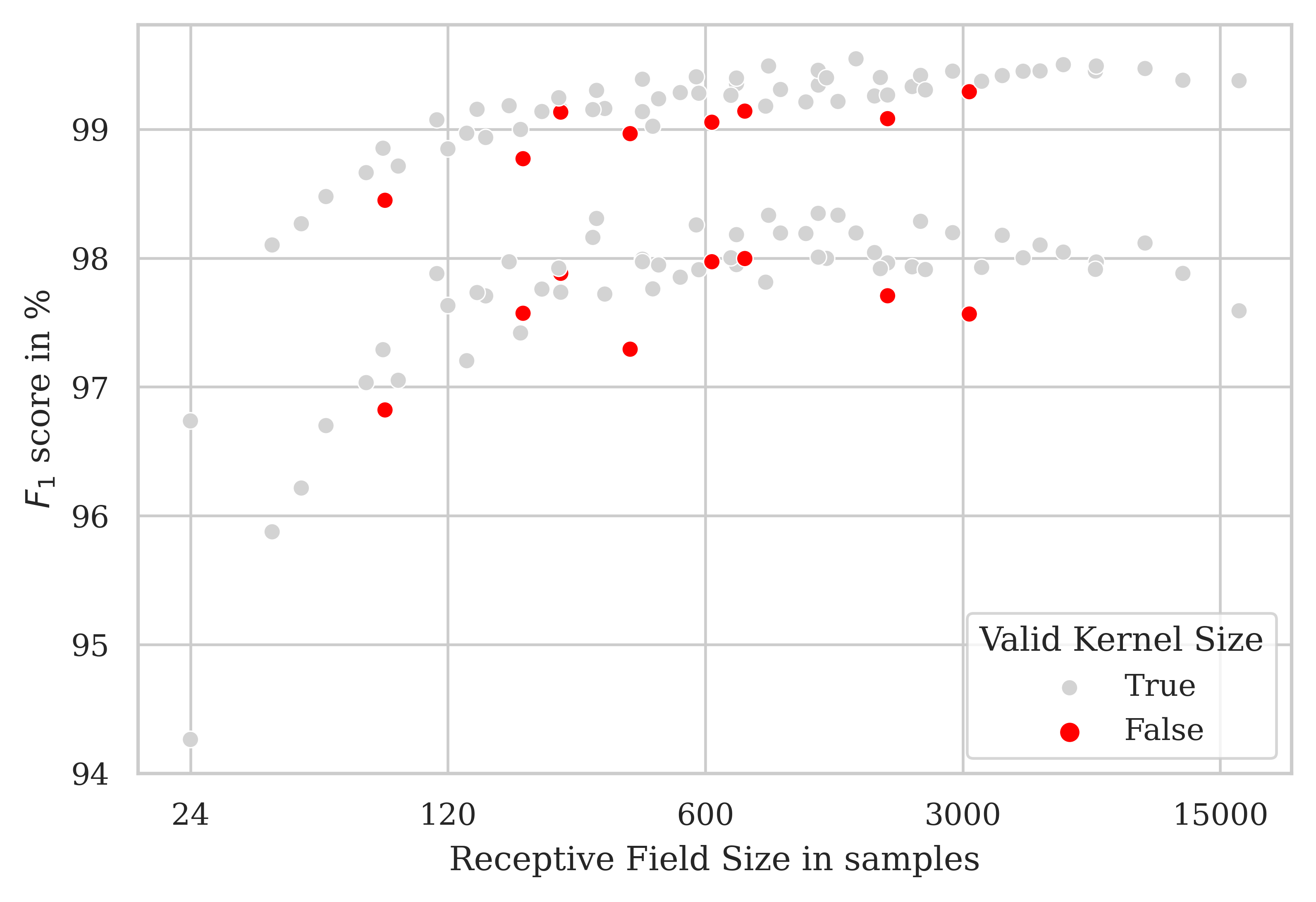
(a) $F_{1}$ scores with models as red dot where kernel size $\leq$ max pooling size.

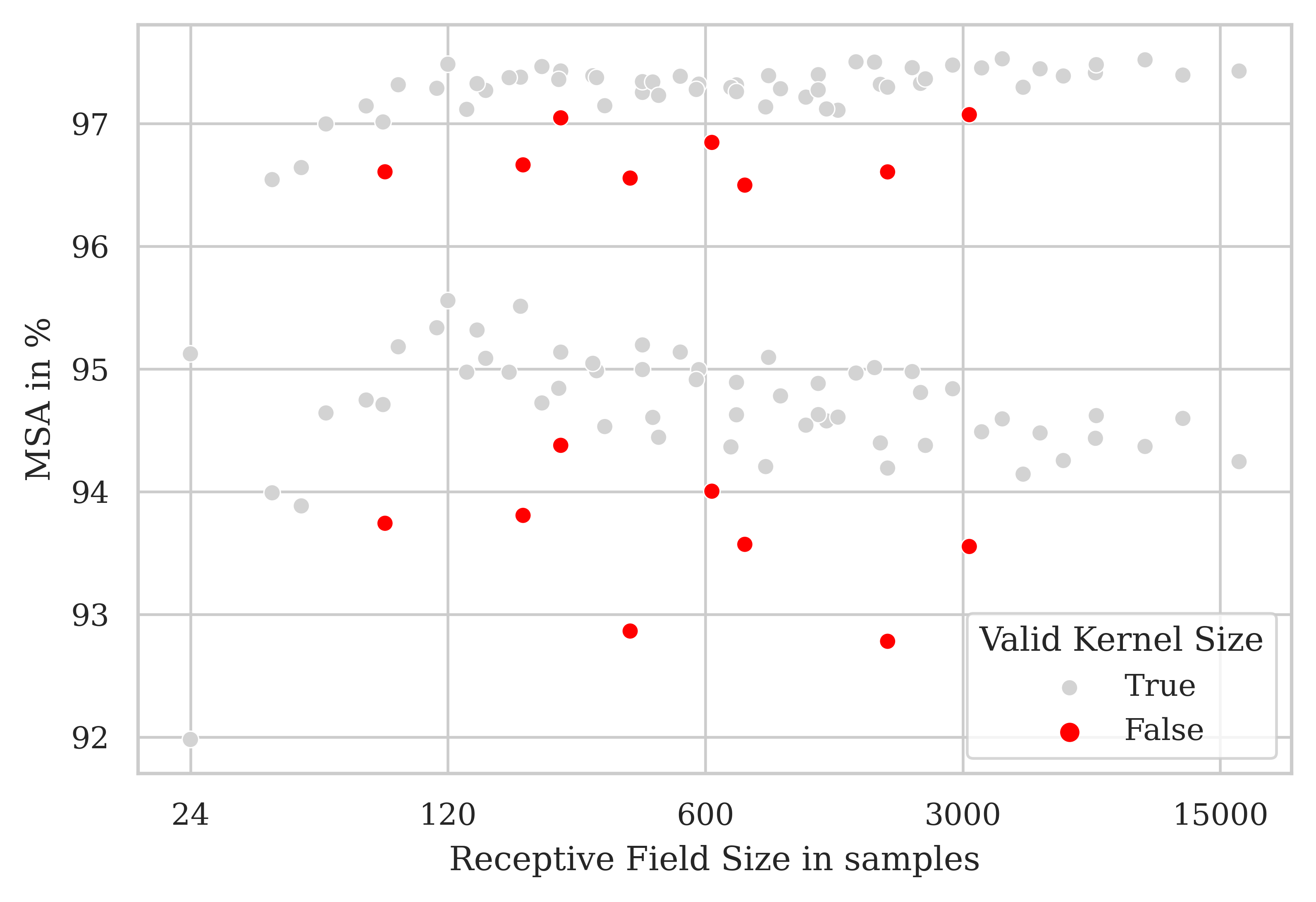
(b) MSA with models as red dot where kernel size $\leq$ max pooling size.

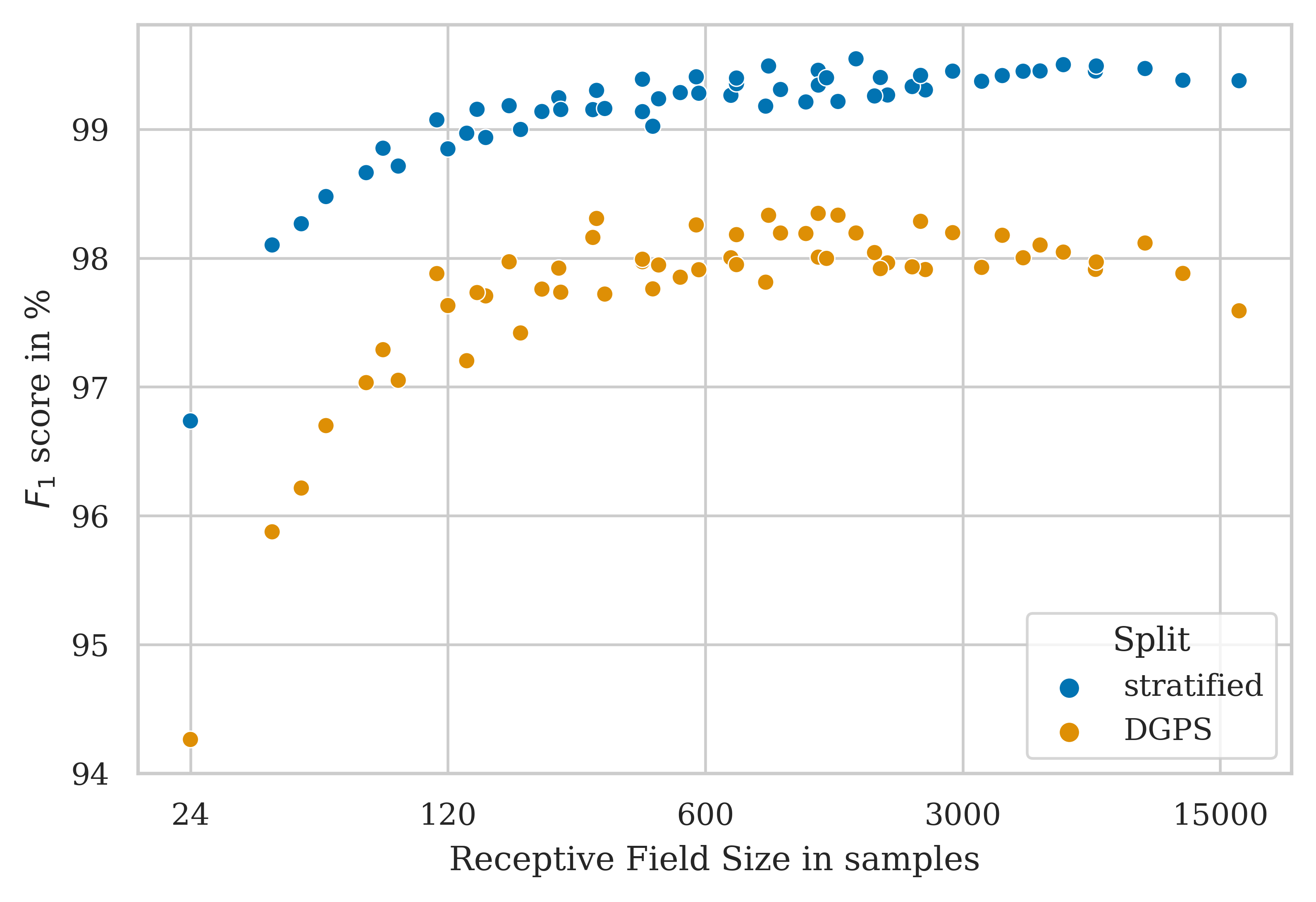
(c) $F_{1}$ scores with only approved hyperparameter combinations.

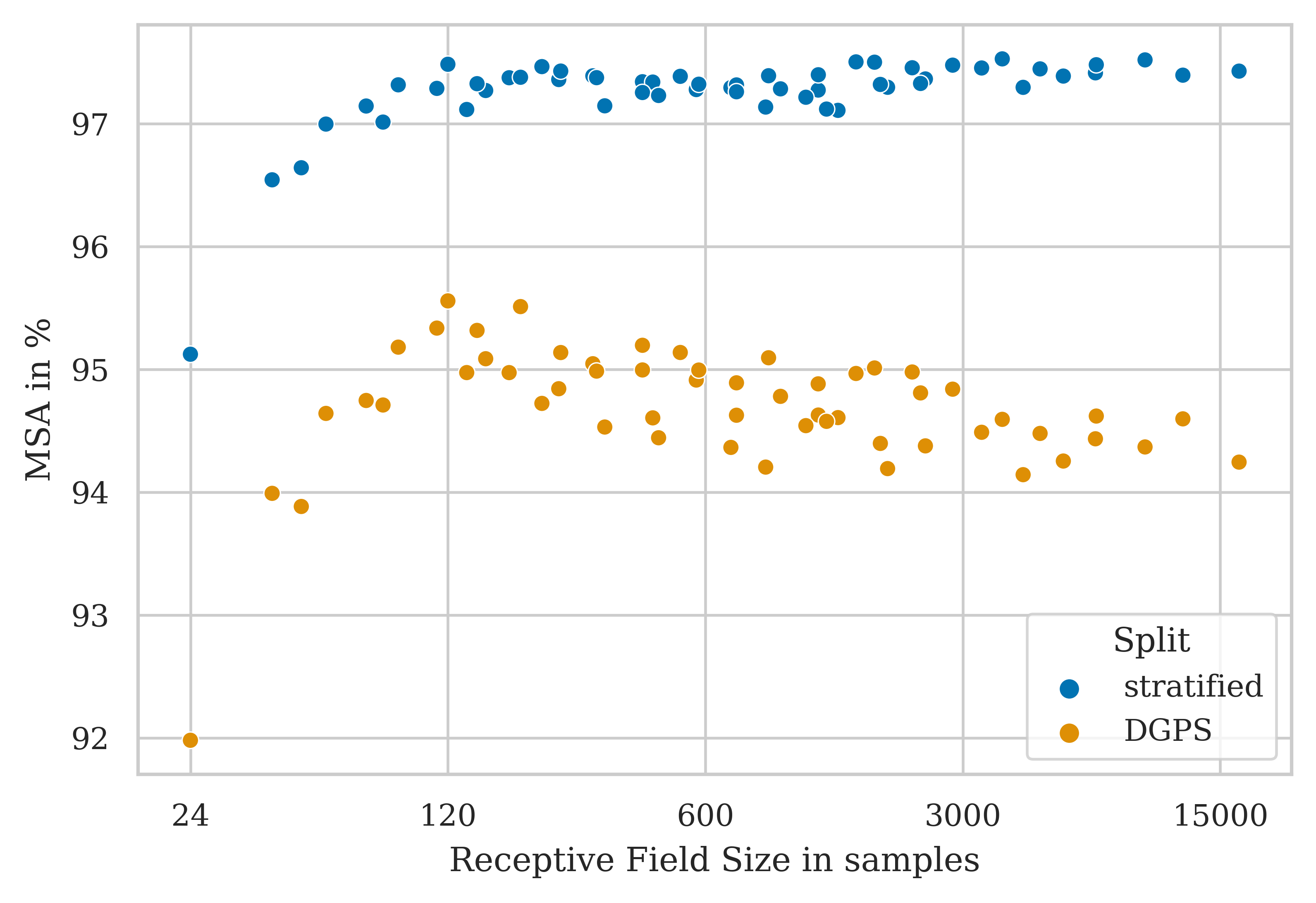
(d) MSA with only approved hyperparameter combinations.

Figure 6: Results of hyperparameter study: $F_{1}$ scores and MSA in dependence of the maximum receptive field trained on DGPS splits.

All models with kernel size $\leq$ max pooling size are therefore excluded from further analyses. With the remaining models, a clear correlation between receptive field size and result is evident for both $F_{1}$ score (fig. 6(c)) and MSA (fig. 6(d)). For the $F_{1}$ score, a disadvantage due to large receptive fields is not clearly recognisable. For MSA, on the other hand, a clear peak is recognisable at around 120 samples. For larger receptive fields, a plateau (stratified split) or a drop (DGPS split) in the results is evident. This could be explained by the larger max pooling size of the models with larger receptive fields, since it increasingly loses temporal information with size.

To select the final hyperparameters for VADERraw, the harmonic mean was determined from the $F_{1}$ score and the MSA for both splits (fig. 7). This is to ensure that the hyperparameters deliver good results in all metrics and scenarios. A closer look at the results shows that the best results are achieved with 4 pooling steps (fig. 7(a)). This could be due to the fact that this increases the complexity of the model, as the data is additionally filtered twice (once in the encoder path and once in the decoder path) with each pooling step. The best results are achieved with a max pooling size of 3 (fig. 7(b)). This could be because it allows a larger receptive field than a max pooling size of 2, but does not lose as much information as max pooling sizes of 4 or 5. The impact of the kernel size is the most ambiguous (fig. 7(c)). There are slight tendencies towards medium kernel sizes of 7-15, but only extreme cases such as a kernel size of 27 can be ruled out.

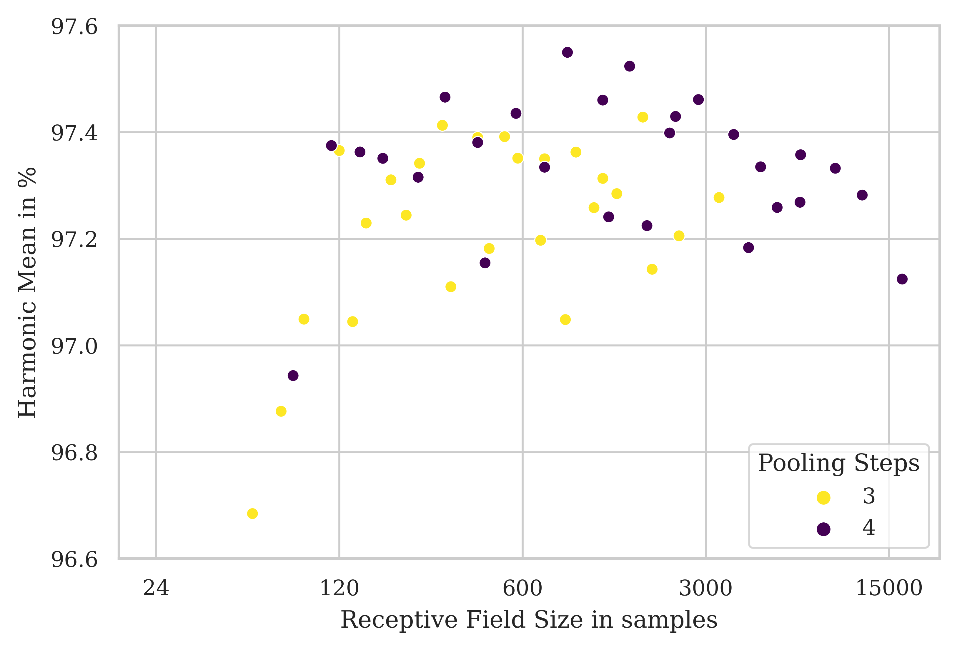
(a) Importance of amount of pooling steps.

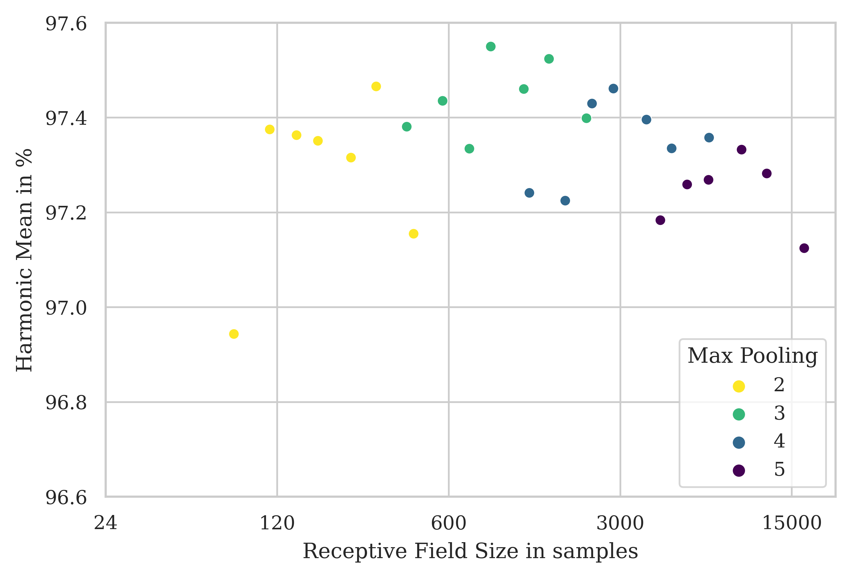
(b) Importance of max pooling size. Only hyperparameter combinations with 4 pooling steps.

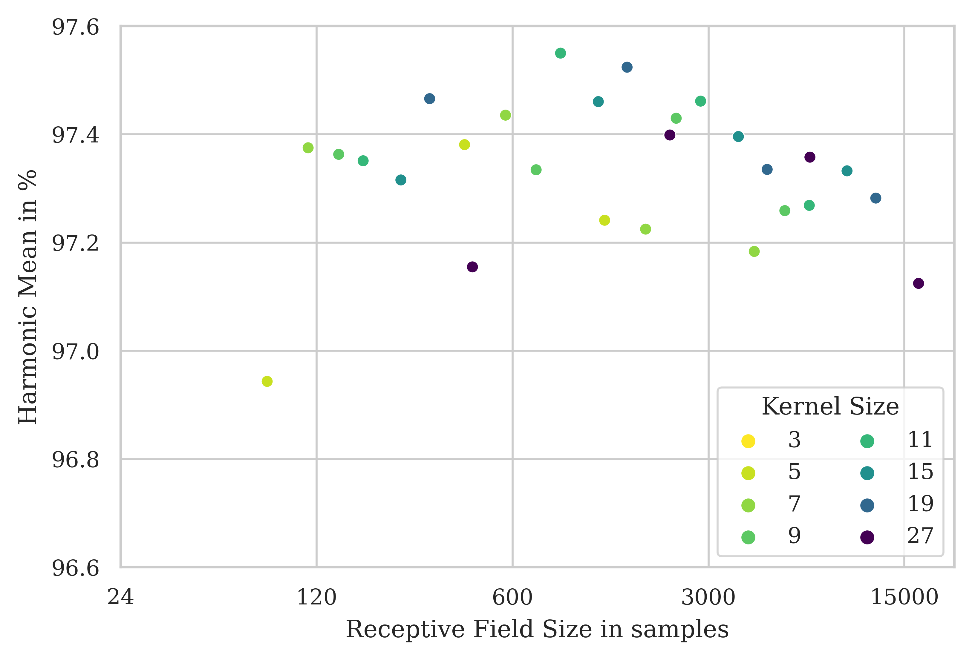
(c) Importance of kernel size. Only hyperparameter combinations with 4 pooling steps.

l

Figure 7: Harmonic mean of $F_{1}$ score and MSA for both splits as a function of receptive field size.

For the final evaluation, the optimal hyperparameter combination with four pooling steps, max pooling size of three and a kernel size of nine, resulting in a receptive field size of 729 samples, is selected as the first VADERraw model. In order to test the hypothesis that the model must be able to map a maximum of 5 Hz with a load-dependent natural frequency of the bridge, the combination was selected that comes closest to this by changing only a single hyperparameter. The second VADERraw model thus differs only in the max pooling size with a value of two instead of three, yielding a receptive field size of 243 samples. From here on, the max pooling size is appended to the model name for traceability, so that the first model is called VADERraw3 and the second model VADERraw2.

Validation Results: The VADERraw models have similar results for both splits (fig. 8). For $F_{1}$ score, VADERraw2 is usually slightly worse than VADERraw3 for the training and validation data (fig. 8(a), 8(c)). No clear differences are recognisable for the loss. VADERspec performs worse than the VADERraw models in all cases. It is particularly noticeable here that the loss of VADERspec on the training data is similar to that of the VADERraw models but significantly worse on the validation data (fig. 8(b), 8(d)). Spectograms as input therefore appear to increase the risk of overfitting. A comparable tendency can also be seen in the $F_{1}$ score, where VADERspec would probably perform just as well on the training data with longer training, but performs significantly worse on the validation data than the VADERraw models.

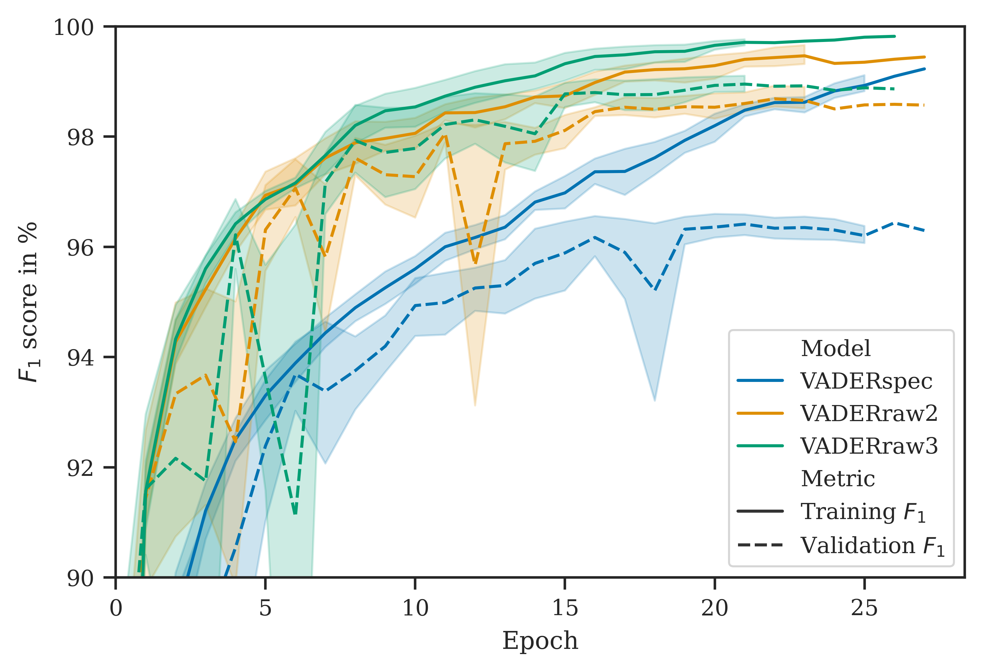
(a) DGPS splits: $F_{1}$ scores in  %.

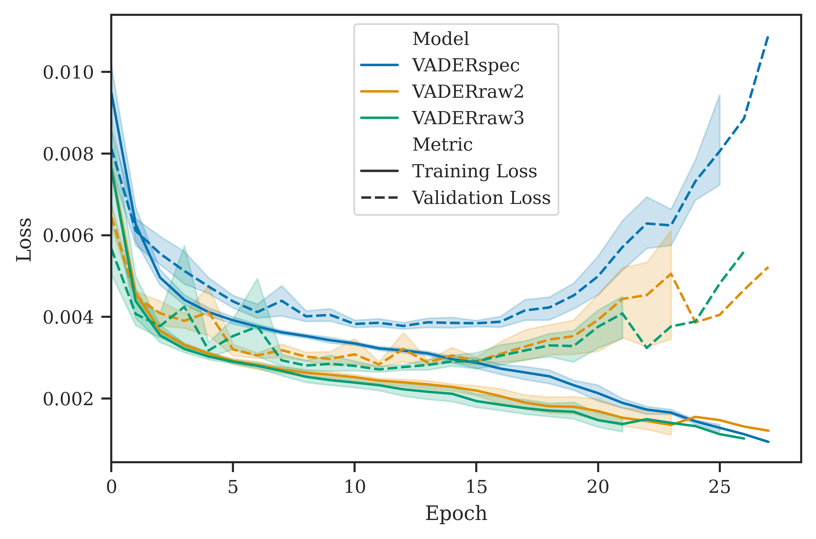
(b) DGPS splits: Binary Focal Loss with $\gamma=2.5$.

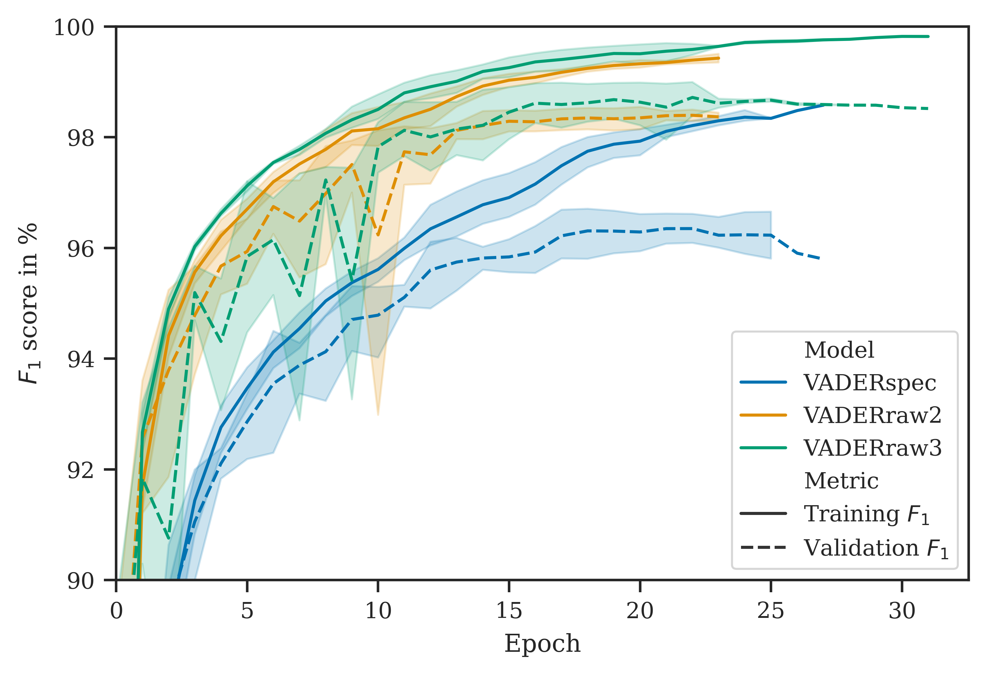
(c) Stratified splits: $F_{1}$ scores in  %.

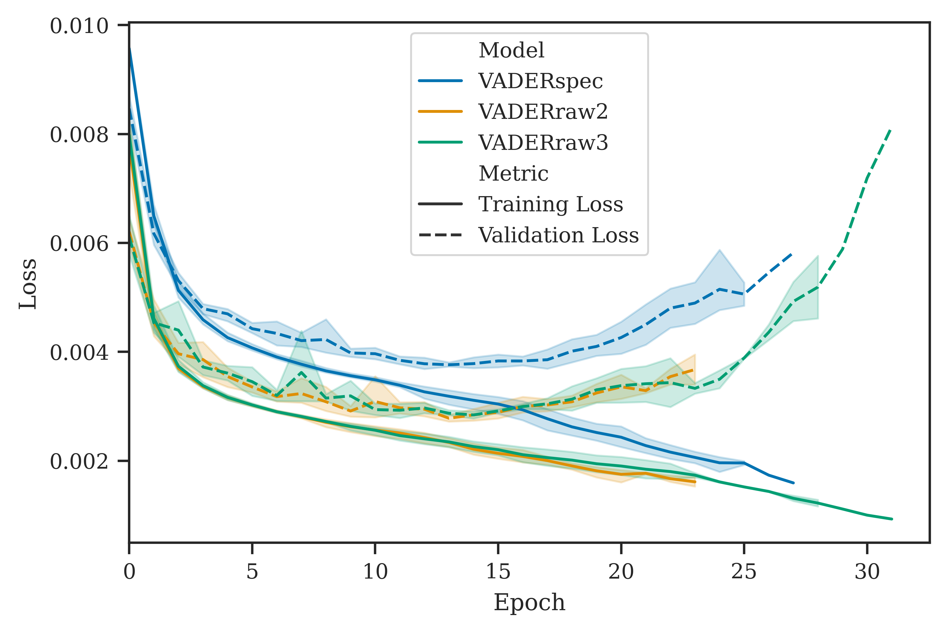
(d) Stratified splits: Binary Focal Loss with $\gamma=2.5$.

Figure 8: Results on training and validation data per epoch with confidence interval with a coefficient of 95 % determined over the five folds.

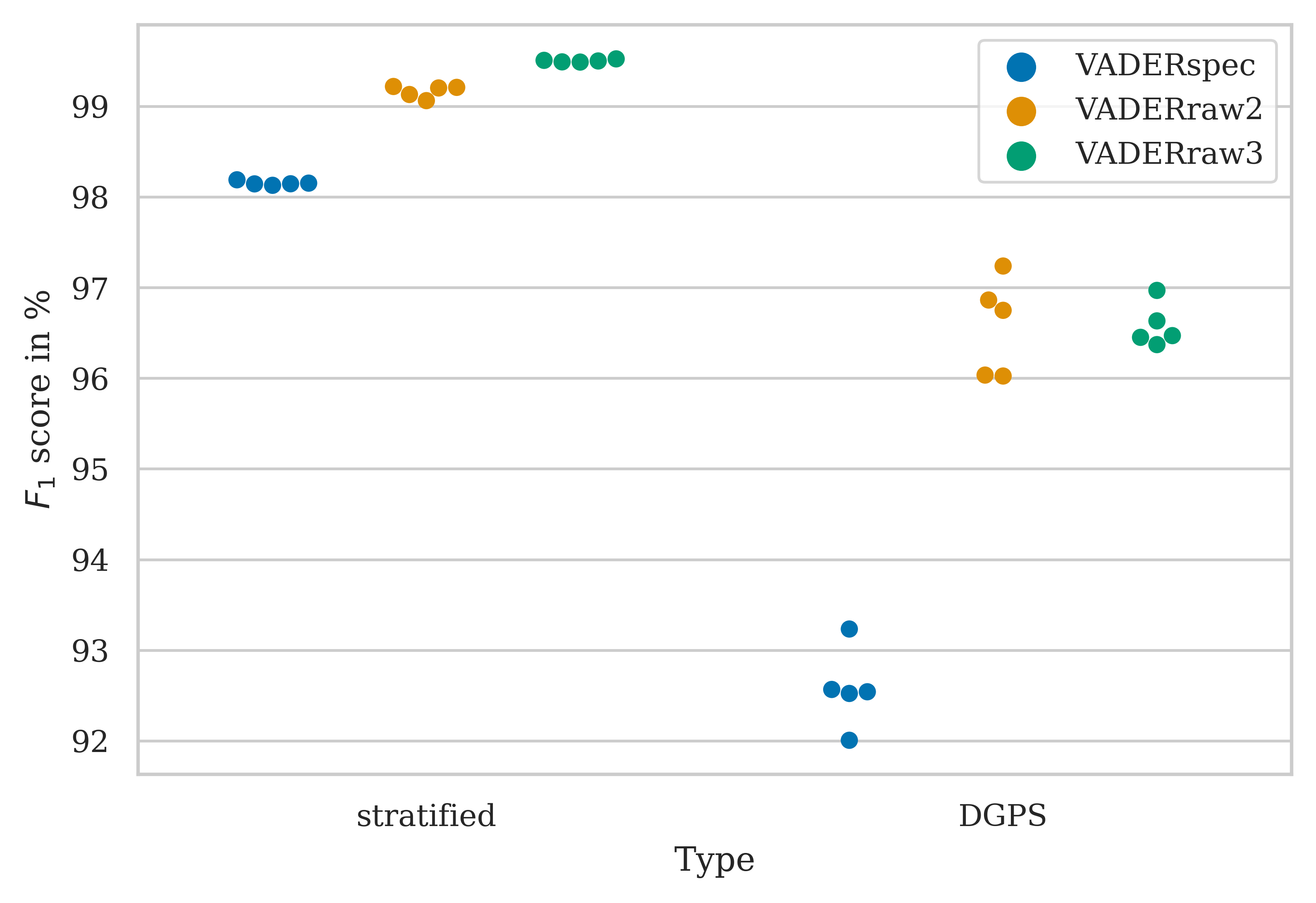
(a) $F_{1}$ score

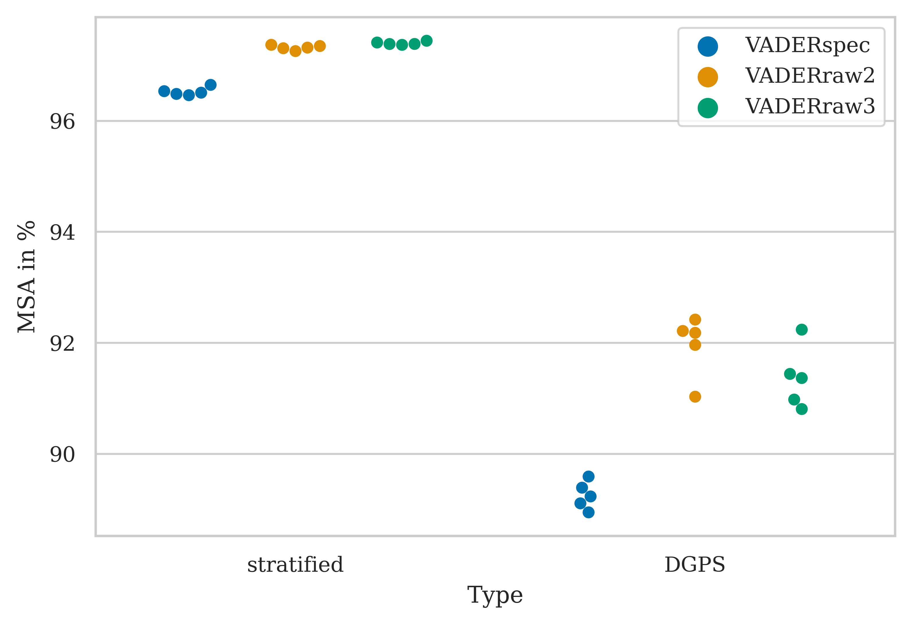
(b) MSA

Figure 9: $F_{1}$ score and MSA of the models for the two types of data split on the test sets. One data point was calculated per sensor, train and fold.

While the loss is calculated per sample and therefore only counts exact hits (exact time at which an axle passes the respective sensor), the $F_{1}$ score is calculated per train axle. Thus, it can be interpreted that for all models and scenarios, the frequency of exact hits decreases again from about halfway through the training, but in return more axles are recognised. Therefore, depending on the boundary condition, either the loss or the $F_{1}$ score can be selected as the criterion for terminating the training.

Test results: For the test results of the models, the learned parameters from the epoch with the best $F_{1}$ score on the validation set were chosen. Using these parameters, the models were then evaluated on the previously unseen test set. This procedure was repeated for all folds, splits (stratified and DGPS) and thresholds (200 cm and 37 cm) for each of the three models (VADERspec, VADERraw2 and VADERraw3). The VADERraw models achieve significantly higher accuracy for both threshold values (200 cm and 37 cm) and both splits (stratified and DGPS) (fig. 9(a), 9(b)). In general, it can be observed that the accuracy of all models is considerably better for the stratified split compared to the DGPS split. The variance of the results is comparable for all models and as expected, the variance is generally higher for the more difficult DGPS scenario. VADERraw2 achieves the best results in all metrics for the DGPS splits while VADERraw3 achieves the best results for the stratified splits (tab. 2). Since VADERraw3 has a significantly larger receptive field, it could be that the model learns entire train axle configurations, while VADERraw2 only learns individual axles or bogies. In this case, this would be advantageous for a representative data set (stratified splits), while it would increase the overfitting on the training data for non-representative data (DGPS splits). Generally VADERraw3 and VADERraw2 achieve similar results and only VADERspec performs significantly worse.

Type	Model	$\bar{\Delta s}$	$F_{1}$
			200 cm	37 cm
DGPS	VADERspec	21.5 cm	92.6 %	75.6 %
	VADERraw2	16.1 cm	96.6 %	83.4 %
	VADERraw3	17.3 cm	96.6 %	82.7 %
stratified	VADERspec	6.95 cm	98.2 %	94.3 %
	VADERraw2	5.36 cm	99.2 %	96.5 %
	VADERraw3	5.21 cm	99.5 %	96.8 %

Table 2: $F_{1}$ score and $\bar{\Delta s}$ calculated for all samples of the corresponding folds.

Sensor dependent test results: It was previously observed that one of the sensors of the measurement campaign was degraded [37]. To investigate the influence of sensor degradation for each model and split more closely, the $F_{1}$ score for both threshold values and both splits (fig. 10(a) to 10(d)), and the MSA for both splits with a threshold value of 200 cm (fig. 10(e), 10(f)) were examined per sensor. Generally, VADERraw performs better than VADERspec in all quantiles across all plots. It is noteworthy that, for the DGPS splits, the difference from sensor R3 to the other sensors is smaller.

In general, it is clearly visible that worse results are achieved on sensor R3 (fig. 10). The difference is most striking for the stratified splits, because in the majority of cases even the lower quartile is 100 % and the results only scatter widely for sensor R3. For the DGPS splits, the results are more scattered for all senors, but there are still large differences, especially in the median. it is also noticeable that VADERspec consistently performs worst and the VADERraw models are close to each other. For sensor R3, VADERraw3 almost always performs better than VADERraw2, but due to the high dispersion of the results, this is not necessarily due to the model. Evaluating the results again, excluding sensor R3, VADERraw2 now performs best in all metrics and scenarios (tab. 3. At a threshold of 200 cm, 99.9 % of the axles are now recognized with a $\bar{\Delta s}$ of only 3.69 cm. Therefore, the RF rule seems to be confirmed for fully functioning sensors. In the case of sensor degradation, larger receptive fields appear to have some advantages (tab. 2), although the differences here are dependent on the scenario.

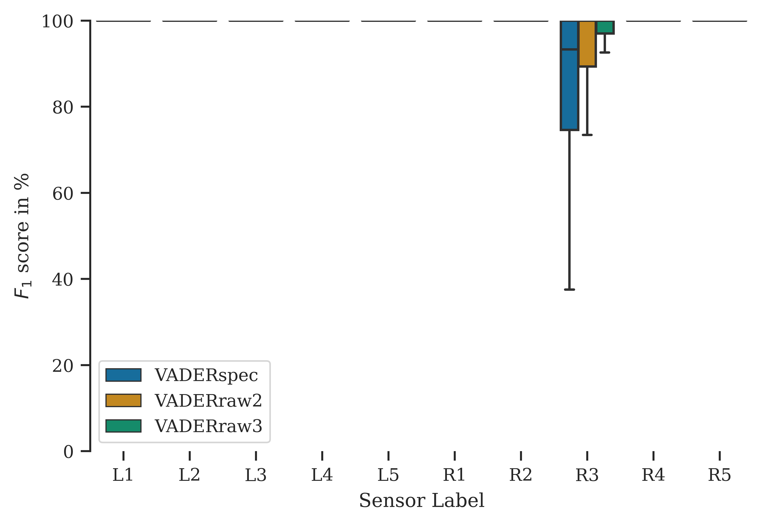
(a) $F_{1}$ score with a threshold of 200 cm for each sensor trained with the stratified splits.

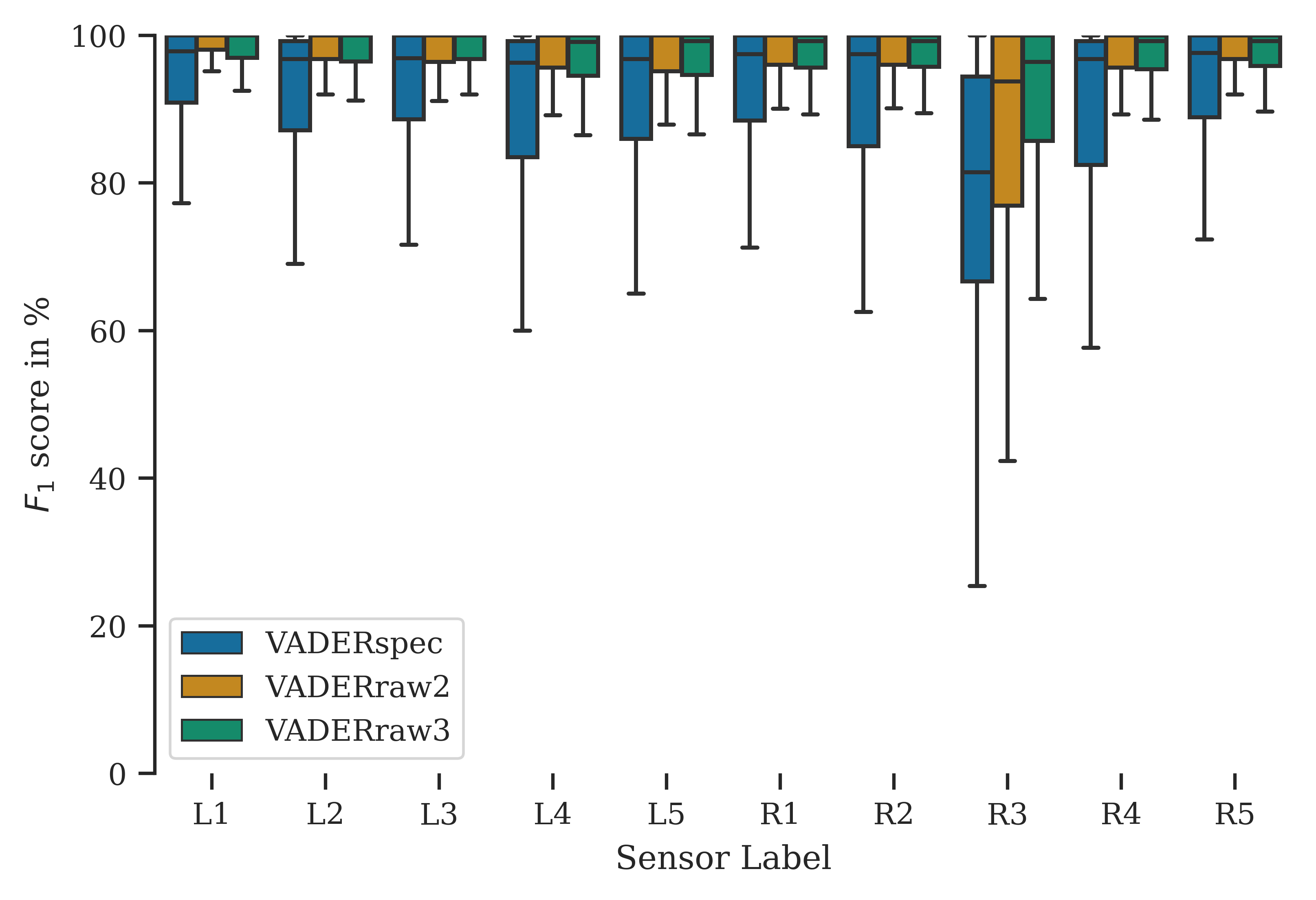
(b) $F_{1}$ score with a threshold of 200 cm for each sensor trained with the DGPS splits.

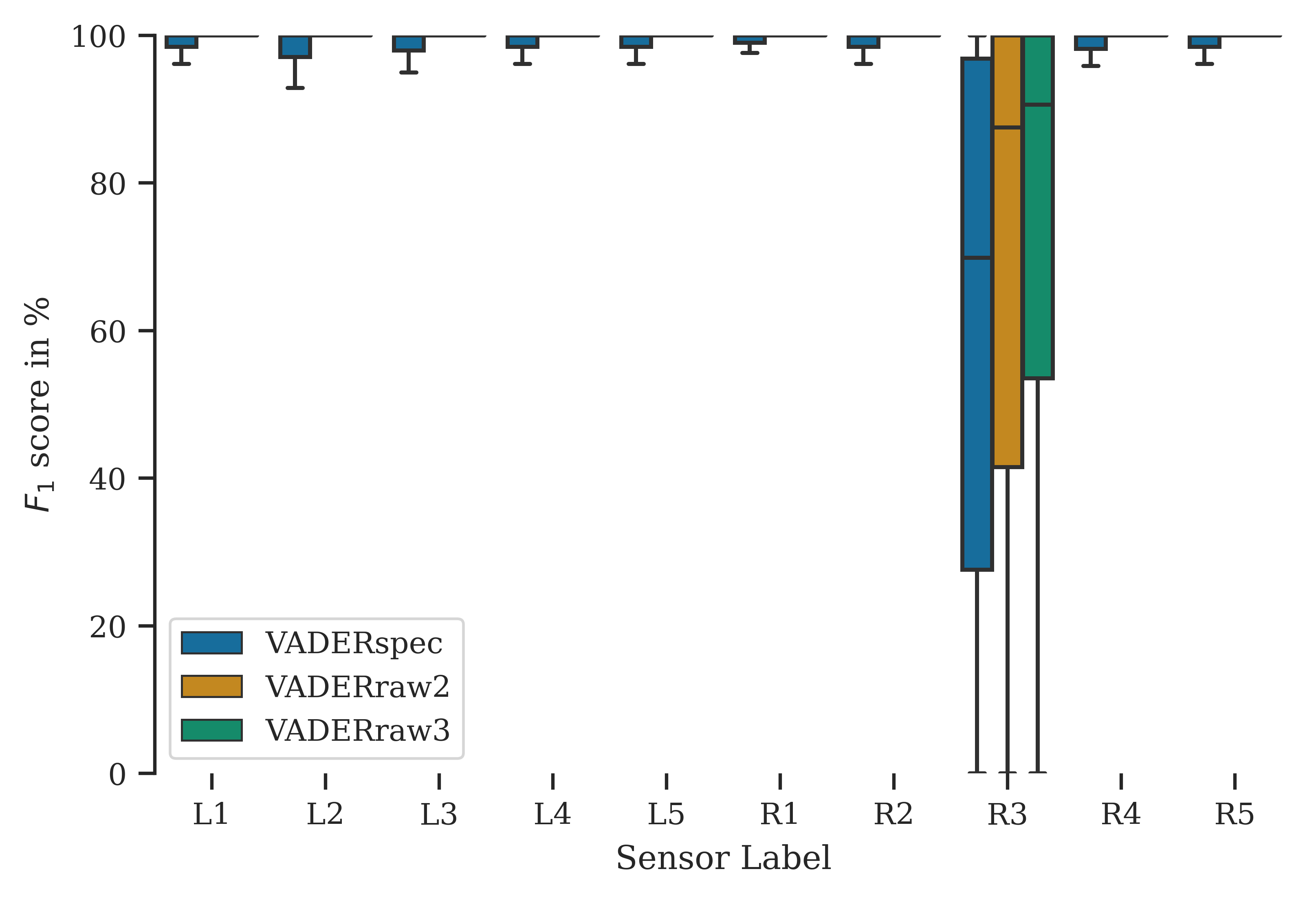
(c) $F_{1}$ score with a threshold of 37 cm for each sensor trained with the stratified splits.

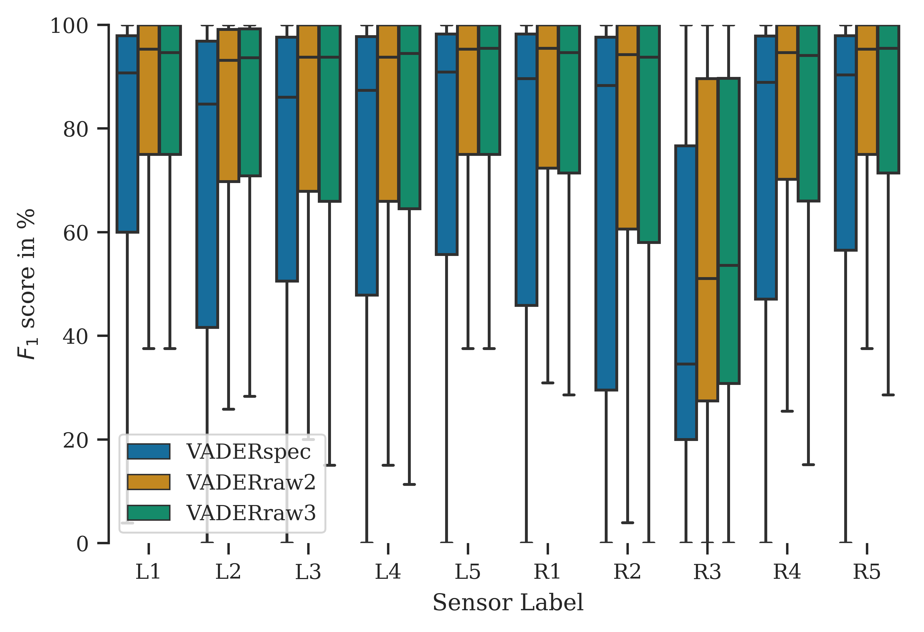
(d) $F_{1}$ score with a threshold of 37 cm for each sensor trained with DGPS splits.

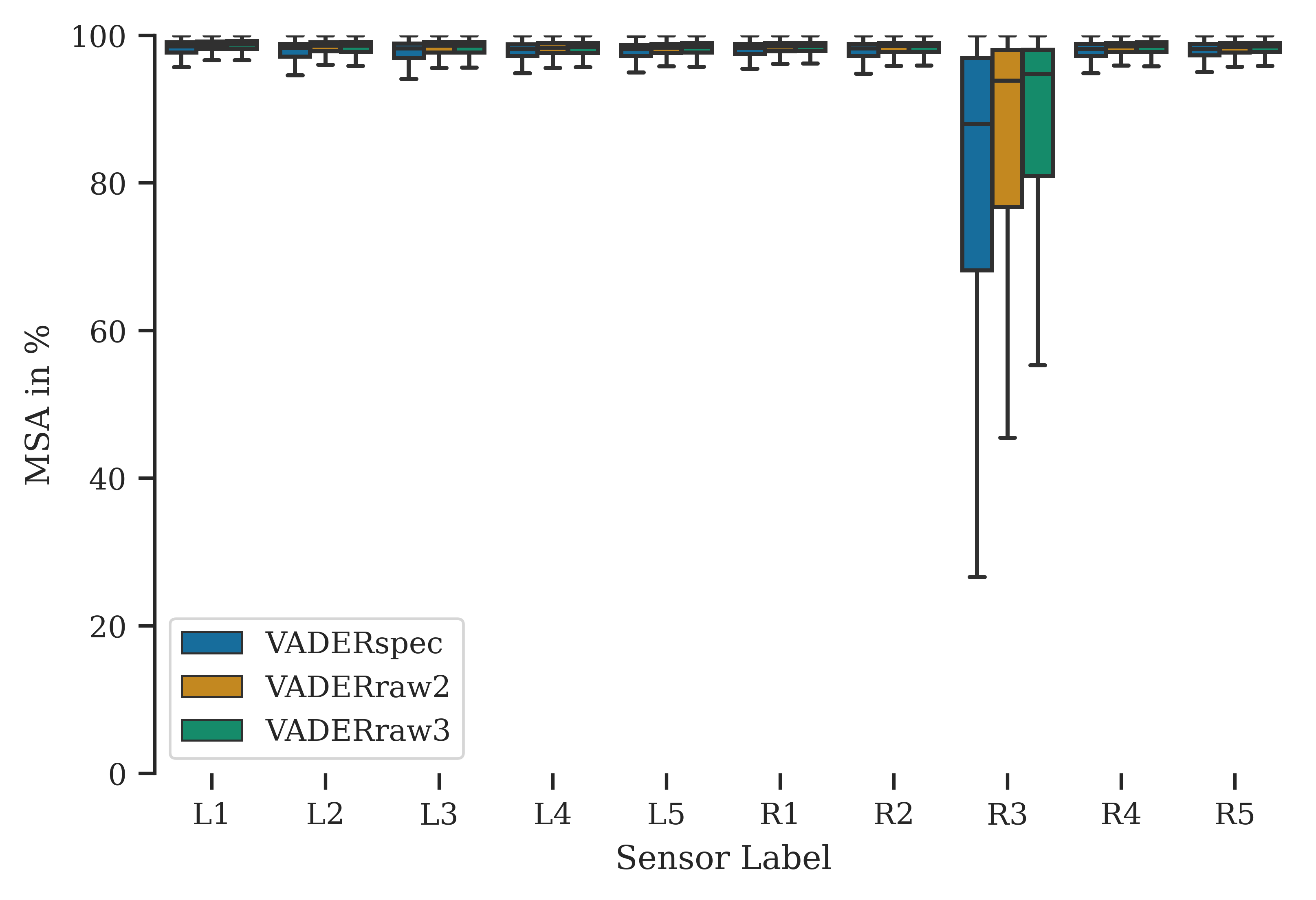
(e) MSA for each sensor trained with stratified splits.

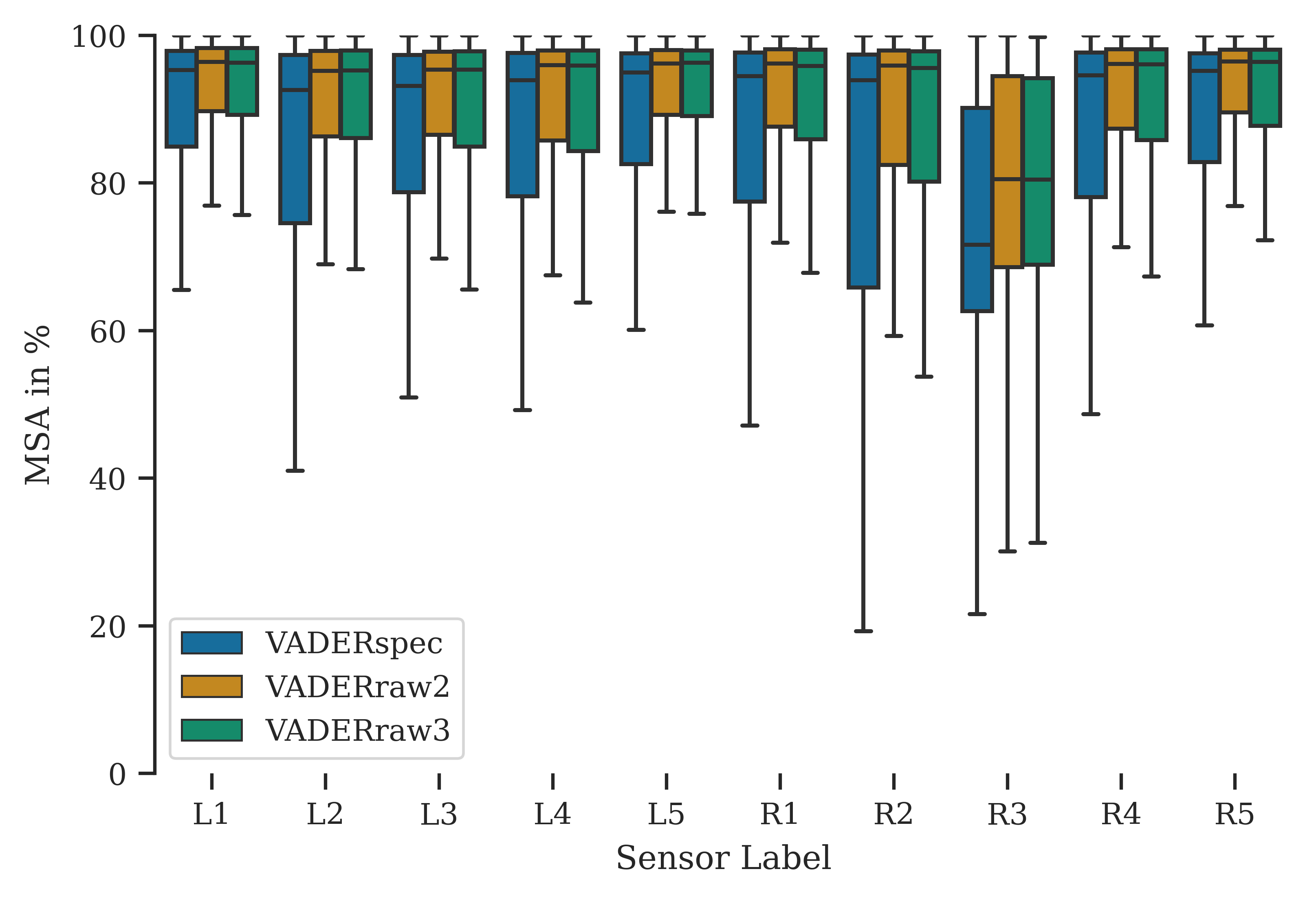
(f) MSA for each sensor trained with DGPS splits.

Figure 10: Metrics evaluated per sensor.

Type	Model	$\bar{\Delta s}$	$F_{1}$
			200 cm	37 cm
DGPS	VADERspec	19.6 cm	93.9 %	78.4 %
	VADERraw2	14.5 cm	97.5 %	85.8 %
	VADERraw3	15.6 cm	97.1 %	85.0 %
stratified	VADERspec	5.00 cm	99.4 %	97.5 %
	VADERraw2	3.69 cm	99.9 %	99.1 %
	VADERraw3	3.71 cm	99.9 %	98.9 %

Table 3: $F_{1}$ score and $\bar{\Delta s}$ calculated for all samples of the corresponding folds without sensor R3.

4 Conclusion

We have demonstrated that an CNN with an adequate receptive field can achieve better results using raw data compared to using a spectrogram as input. This could be due to the loss of information when transforming into spectograms, whereas an CNN can directly learn to filter the data comparable to it when necessary. In order to achieve comparable or better results with raw data instead of spectograms, we propose the RF rule to calculate the required size of the largest receptive field of a model (eq. 1). Based on our results we were able to show the potential of raw data as input considering the RF rule.

Furthermore, we demonstrated that acceleration data is suitable for axle detection and localisation. It is particularly noteworthy that even when training with only one type of train and thus a non-representative training set, we were able to achieve very good results on other train types, demonstrating that the model generalises exceptionally well. In this case, VADER was trained solely on trains with 32 axles but could still detect 97.5 % of the axles of all other train types, with an average spatial error of 14.5 cm. Trained on a representative training set, VADER was able to detect 99.9 % of the axles with an error of just 3.69 cm. In addition to improved accuracy, VADER using raw data allows for an inference that is 65 times faster while using only 1 % of the memory. This makes the use of virtual axle detectors in real time and using edge computing possible for the first time.

It is evident that there is significant potential yet to be unlocked. The VADER model evaluates the signals of the acceleration sensors individually. A joint evaluation of the signals could further increase the accuracy. Another approach could be a combination of raw input data, FCN-based spectrogram-like data transformation, and transformer-based classification. This way, the FCN could learn how to optimally transform the data, while the transformer model would be utilised to identify even more complex correlations and relationships.

Author Contributions

Henrik Riedel: Conceptualization, investigation, methodology, software, validation, visualization and writing - original draft. Steven Robert Lorenzen: Funding, supervision and writing - review & editing Clemens Hübler: Resources, supervision and writing - review & editing.

Data and Source Code

The data [54] as well as the source code [55] used in this paper is published and contains:

1. All measurement data

2. Matlab code to label data and save as text files

3. Python code for transformation, training, evaluation and plotting.

References

- CHAN et al. [2001] T. CHAN, L. YU, S. LAW, T. YUNG, Moving force identification studies, i: Theory, Journal of Sound and Vibration 247 (2001) 59–76. URL: https://www.sciencedirect.com/science/article/pii/S0022460X01936302. doi:https://doi.org/10.1006/jsvi.2001.3630.
- Kazemi Amiri and Bucher [2017] A. Kazemi Amiri, C. Bucher, A procedure for in situ wind load reconstruction from structural response only based on field testing data, Journal of Wind Engineering and Industrial Aerodynamics 167 (2017) 75–86. URL: https://www.sciencedirect.com/science/article/pii/S0167610516303452. doi:https://doi.org/10.1016/j.jweia.2017.04.009.
- Hwang et al. [2009] J. Hwang, A. Kareem, W. Kim, Estimation of modal loads using structural response, Journal of Sound and Vibration 326 (2009) 522–539. URL: https://www.sciencedirect.com/science/article/pii/S0022460X09004271. doi:https://doi.org/10.1016/j.jsv.2009.05.003.
- Lourens et al. [2012] E. Lourens, C. Papadimitriou, S. Gillijns, E. Reynders, G. De Roeck, G. Lombaert, Joint input-response estimation for structural systems based on reduced-order models and vibration data from a limited number of sensors, Mechanical Systems and Signal Processing 29 (2012) 310–327. URL: https://www.sciencedirect.com/science/article/pii/S088832701200012X. doi:https://doi.org/10.1016/j.ymssp.2012.01.011.
- Firus [2022] A. Firus, A contribution to moving force identification in bridge dynamics, Ph.D. thesis, Technische Universität, Darmstadt, 2022. URL: http://tuprints.ulb.tu-darmstadt.de/20293/. doi:https://doi.org/10.26083/tuprints-00020293.
- Firus et al. [2022] A. Firus, R. Kemmler, H. Berthold, S. Lorenzen, J. Schneider, A time domain method for reconstruction of pedestrian induced loads on vibrating structures, Mechanical Systems and Signal Processing 171 (2022) 108887. URL: https://www.sciencedirect.com/science/article/pii/S0888327022000772. doi:https://doi.org/10.1016/j.ymssp.2022.108887.
- Lydon et al. [2017] M. Lydon, D. Robinson, S. E. Taylor, G. Amato, E. J. O. Brien, N. Uddin, Improved axle detection for bridge weigh-in-motion systems using fiber optic sensors, Journal of Civil Structural Health Monitoring 7 (2017) 325–332. URL: https://link.springer.com/article/10.1007/s13349-017-0229-4. doi:10.1007/s13349-017-0229-4.
- Wang et al. [2019] H. Wang, Q. Zhu, J. Li, J. Mao, S. Hu, X. Zhao, Identification of moving train loads on railway bridge based on strain monitoring, Smart Structures and Systems 23 (2019) 263–278. URL: https://koreascience.or.kr/article/JAKO201913457807828.page. doi:10.12989/sss.2019.23.3.263.
- Yu et al. [2016] Y. Yu, C. Cai, L. Deng, State-of-the-art review on bridge weigh-in-motion technology, Advances in Structural Engineering 19 (2016) 1514–1530. URL: http://journals.sagepub.com/doi/10.1177/1369433216655922. doi:10.1177/1369433216655922.
- He et al. [2019] W. He, T. Ling, E. J. OBrien, L. Deng, Virtual axle method for bridge weigh-in-motion systems requiring no axle detector, Journal of Bridge Engineering 24 (2019) 04019086. URL: {https://ascelibrary.org/doi/abs/10.1061/%28ASCE%29BE.1943-5592.0001474}. doi:10.1061/(ASCE)BE.1943-5592.0001474.
- O’Brien et al. [2012] E. J. O’Brien, D. Hajializadeh, N. Uddin, D. Robinson, R. Opitz, Strategies for Axle Detection in Bridge Weigh-in-Motion Systems, in: Proceedings of the International Conference on Weigh-In-Motion, June, 2012, pp. 79–88. URL: https://www.researchgate.net/publication/281031765_STRATEGIES_FOR_AXLE_DETECTION_IN_BRIDGE_WEIGH-IN-MOTION_SYSTEMS.
- Zhao et al. [2020] H. Zhao, C. Tan, E. J. OBrien, N. Uddin, B. Zhang, Wavelet-based optimum identification of vehicle axles using bridge measurements, Applied Sciences 10 (2020). URL: https://www.mdpi.com/2076-3417/10/21/7485. doi:10.3390/app10217485.
- Thater et al. [1998] G. Thater, P. Chang, D. R. Schelling, C. C. Fu, Estimation of bridge static response and vehicle weights by frequency response analysis, Canadian Journal of Civil Engineering 25 (1998) 631–639. URL: https://cdnsciencepub.com/doi/10.1139/l97-128. doi:10.1139/l97-128.
- Zakharenko et al. [2022] M. Zakharenko, G. T. Frøseth, A. Rönnquist, Train classification using a weigh-in-motion system and associated algorithms to determine fatigue loads, Sensors 22 (2022). URL: https://www.mdpi.com/1424-8220/22/5/1772. doi:10.3390/s22051772.
- Bernas et al. [2018] M. Bernas, B. Płaczek, W. Korski, P. Loska, J. Smyła, P. Szymała, A survey and comparison of low-cost sensing technologies for road traffic monitoring, Sensors 18 (2018). URL: https://www.mdpi.com/1424-8220/18/10/3243. doi:10.3390/s18103243.
- Kouroussis et al. [2015] G. Kouroussis, C. Caucheteur, D. Kinet, G. Alexandrou, O. Verlinden, V. Moeyaert, Review of trackside monitoring solutions: From strain gages to optical fibre sensors, Sensors 15 (2015) 20115–20139. URL: https://www.mdpi.com/1424-8220/15/8/20115. doi:10.3390/s150820115.
- Lydon et al. [2016] M. Lydon, S. E. Taylor, D. Robinson, A. Mufti, E. J. O. Brien, Recent developments in bridge weigh in motion (b-wim), Journal of Civil Structural Health Monitoring 6 (2016) 69–81. URL: https://link.springer.com/article/10.1007/s13349-015-0119-6. doi:10.1007/s13349-015-0119-6.
- Tan et al. [2023] C. Tan, B. Zhang, H. Zhao, N. Uddin, H. Guo, B. Yan, An extended bridge weigh-in-motion system without vehicular axles and speed detectors using nonnegative lasso regularization, Journal of Bridge Engineering 28 (2023) 04023022. URL: https://ascelibrary.org/doi/abs/10.1061/JBENF2.BEENG-5864. doi:10.1061/JBENF2.BEENG-5864. arXiv:https://ascelibrary.org/doi/pdf/10.1061/JBENF2.BEENG-5864.
- Mesaros et al. [2021] A. Mesaros, T. Heittola, T. Virtanen, M. D. Plumbley, Sound event detection: A tutorial, IEEE Signal Processing Magazine 38 (2021) 67–83. doi:10.1109/MSP.2021.3090678.
- Mesaros et al. [2019] A. Mesaros, A. Diment, B. Elizalde, T. Heittola, E. Vincent, B. Raj, T. Virtanen, Sound event detection in the dcase 2017 challenge, IEEE/ACM Transactions on Audio, Speech, and Language Processing 27 (2019) 992–1006. doi:10.1109/TASLP.2019.2907016.
- Chan and Chin [2020] T. K. Chan, C. S. Chin, A comprehensive review of polyphonic sound event detection, IEEE Access 8 (2020) 103339–103373. doi:10.1109/ACCESS.2020.2999388.
- Wang et al. [2020] Y. Wang, J. Salamon, N. J. Bryan, J. Pablo Bello, Few-shot sound event detection, in: ICASSP 2020 - 2020 IEEE International Conference on Acoustics, Speech and Signal Processing (ICASSP), 2020, pp. 81–85. doi:10.1109/ICASSP40776.2020.9054708.
- Latif et al. [2021] S. Latif, R. Rana, S. Khalifa, R. Jurdak, J. Qadir, B. W. Schuller, Deep representation learning in speech processing: Challenges, recent advances, and future trends, 2021. arXiv:2001.00378.
- Purwins et al. [2019] H. Purwins, B. Li, T. Virtanen, J. Schlüter, S.-Y. Chang, T. Sainath, Deep learning for audio signal processing, IEEE Journal of Selected Topics in Signal Processing 13 (2019) 206–219. doi:10.1109/JSTSP.2019.2908700.
- Radford et al. [2023] A. Radford, J. W. Kim, T. Xu, G. Brockman, C. Mcleavey, I. Sutskever, Robust speech recognition via large-scale weak supervision, in: A. Krause, E. Brunskill, K. Cho, B. Engelhardt, S. Sabato, J. Scarlett (Eds.), Proceedings of the 40th International Conference on Machine Learning, volume 202 of Proceedings of Machine Learning Research, PMLR, 2023, pp. 28492–28518. URL: https://proceedings.mlr.press/v202/radford23a.html.
- Kiranyaz et al. [2021] S. Kiranyaz, O. Avci, O. Abdeljaber, T. Ince, M. Gabbouj, D. J. Inman, 1d convolutional neural networks and applications: A survey, Mechanical Systems and Signal Processing 151 (2021) 107398. URL: https://www.sciencedirect.com/science/article/pii/S0888327020307846. doi:https://doi.org/10.1016/j.ymssp.2020.107398.
- Arias-Vergara et al. [2021] T. Arias-Vergara, P. Klumpp, J. C. Vasquez-Correa, E. Nöth, J. R. Orozco-Arroyave, M. Schuster, Multi-channel spectrograms for speech processing applications using deep learning methods, Pattern Analysis and Applications 24 (2021) 423–431. URL: https://doi.org/10.1007/s10044-020-00921-5. doi:10.1007/s10044-020-00921-5.
- Bozkurt et al. [2018] B. Bozkurt, I. Germanakis, Y. Stylianou, A study of time-frequency features for cnn-based automatic heart sound classification for pathology detection, Computers in Biology and Medicine 100 (2018) 132–143. URL: https://www.sciencedirect.com/science/article/pii/S0010482518301744. doi:https://doi.org/10.1016/j.compbiomed.2018.06.026.
- Mesaros et al. [2019] A. Mesaros, T. Heittola, T. Virtanen, Acoustic scene classification in dcase 2019 challenge: Closed and open set classification and data mismatch setups, in: Workshop on Detection and Classification of Acoustic Scenes and Events, 2019. doi:10.33682/m5kp-fa97.
- van den Oord et al. [2016] A. van den Oord, S. Dieleman, H. Zen, K. Simonyan, O. Vinyals, A. Graves, N. Kalchbrenner, A. Senior, K. Kavukcuoglu, Wavenet: A generative model for raw audio, 2016. arXiv:1609.03499.
- Ghahremani et al. [2016] P. Ghahremani, V. Manohar, D. Povey, S. Khudanpur, Acoustic modelling from the signal domain using cnns, in: Interspeech 2016, 2016, pp. 3434–3438. URL: http://dx.doi.org/10.21437/Interspeech.2016-1495. doi:10.21437/Interspeech.2016-1495.
- Sailor and Patil [2016] H. B. Sailor, H. A. Patil, Novel unsupervised auditory filterbank learning using convolutional rbm for speech recognition, IEEE/ACM Transactions on Audio, Speech, and Language Processing 24 (2016) 2341–2353. doi:10.1109/TASLP.2016.2607341.
- Chatterjee et al. [2006] P. Chatterjee, E. OBrien, Y. Li, A. González, Wavelet domain analysis for identification of vehicle axles from bridge measurements, Computers & Structures 84 (2006) 1792–1801. URL: https://www.sciencedirect.com/science/article/pii/S0045794906001933. doi:https://doi.org/10.1016/j.compstruc.2006.04.013.
- Kalhori et al. [2017] H. Kalhori, M. M. Alamdari, X. Zhu, B. Samali, S. Mustapha, Non-intrusive schemes for speed and axle identification in bridge-weigh-in-motion systems, Measurement Science and Technology 28 (2017) 025102. URL: https://doi.org/10.1088/1361-6501/aa52ec. doi:10.1088/1361-6501/aa52ec.
- Yu et al. [2017] Y. Yu, C. Cai, L. Deng, Vehicle axle identification using wavelet analysis of bridge global responses, Journal of Vibration and Control 23 (2017) 2830–2840. URL: https://journals.sagepub.com/doi/10.1177/1077546315623147. doi:10.1177/1077546315623147.
- Zhu et al. [2021] Y. Zhu, H. Sekiya, T. Okatani, I. Yoshida, S. Hirano, Acceleration-based deep learning method for vehicle monitoring, IEEE Sensors Journal 21 (2021) 17154–17161. URL: https://ieeexplore.ieee.org/document/9437183. doi:10.1109/JSEN.2021.3082145.
- Lorenzen et al. [2022] S. R. Lorenzen, H. Riedel, M. M. Rupp, L. Schmeiser, H. Berthold, A. Firus, J. Schneider, Virtual axle detector based on analysis of bridge acceleration measurements by fully convolutional network, Sensors 22 (2022). URL: https://www.mdpi.com/1424-8220/22/22/8963. doi:10.3390/s22228963.
- Géron [2019] A. Géron, Hands-on Machine Learning with Scikit-Learn, Keras, and TensorFlow: Concepts, Tools, and Techniques to Build Intelligent Systems, O’Reilly UK Ltd., Sebastopol, 2019. ISBN: 9781492032649.
- Lorenzen et al. [2022] S. R. Lorenzen, H. Riedel, M. Rupp, L. Schmeiser, H. Berthold, A. Firus, J. Schneider, Virtual Axle Detector based on Analysis of Bridge Acceleration Measurements by Fully Convolutional Network, 2022. URL: https://doi.org/10.5281/zenodo.6782319. doi:10.5281/zenodo.6782319.
- Reiterer and Firus [2022] M. Reiterer, A. Firus, Dynamische analyse der zugüberfahrt bei eisenbahnbrücken unter berücksichtigung von nichtlinearen effekten, Beton-und Stahlbetonbau 117 (2022) 90–98.
- Lee et al. [2019] G. R. Lee, R. Gommers, F. Waselewski, K. Wohlfahrt, A. O’Leary, Pywavelets: A python package for wavelet analysis, Journal of Open Source Software 4 (2019) 1237. URL: https://doi.org/10.21105/joss.01237. doi:10.21105/joss.01237.
- Long et al. [2015] J. Long, E. Shelhamer, T. Darrell, Fully convolutional networks for semantic segmentation, in: 2015 IEEE Conference on Computer Vision and Pattern Recognition (CVPR), 2015, pp. 3431–3440. URL: https://ieeexplore.ieee.org/document/7298965. doi:10.1109/CVPR.2015.7298965.
- Ronneberger et al. [2015] O. Ronneberger, P. Fischer, T. Brox, U-net: Convolutional networks for biomedical image segmentation, in: Medical Image Computing and Computer-Assisted Intervention – MICCAI 2015, Springer International Publishing, Cham, 2015, pp. 234–241. URL: https://link.springer.com/chapter/10.1007/978-3-319-24574-4_28. doi:10.1007/978-3-319-24574-4_28.
- Mo et al. [2022] Y. Mo, Y. Wu, X. Yang, F. Liu, Y. Liao, Review the state-of-the-art technologies of semantic segmentation based on deep learning, Neurocomputing 493 (2022) 626–646. URL: https://www.sciencedirect.com/science/article/pii/S0925231222000054. doi:https://doi.org/10.1016/j.neucom.2022.01.005.
- Yu et al. [2023] Y. Yu, C. Wang, Q. Fu, R. Kou, F. Huang, B. Yang, T. Yang, M. Gao, Techniques and challenges of image segmentation: A review, Electronics 12 (2023). URL: https://www.mdpi.com/2079-9292/12/5/1199. doi:10.3390/electronics12051199.
- Siddique et al. [2021] N. Siddique, S. Paheding, C. P. Elkin, V. Devabhaktuni, U-net and its variants for medical image segmentation: A review of theory and applications, IEEE Access 9 (2021) 82031–82057. doi:10.1109/ACCESS.2021.3086020.
- He et al. [2016] K. He, X. Zhang, S. Ren, J. Sun, Deep residual learning for image recognition, in: 2016 IEEE Conference on Computer Vision and Pattern Recognition (CVPR), 2016, pp. 770–778. URL: https://ieeexplore.ieee.org/document/7780459. doi:https://doi.org/10.1109/CVPR.2016.90.
- Wu and He [2020] Y. Wu, K. He, Group normalization, International Journal of Computer Vision 128 (2020) 742–755. URL: https://doi.org/10.1007/s11263-019-01198-w. doi:10.1007/s11263-019-01198-w.
- Lorenzen [2023] S. R. Lorenzen, Railway Bridge Monitoring with Minimal Sensor Deployment: Virtual Sensing and Resonance Curve-Based Drive-by Monitoring, Ph.D. thesis, Technische Universität Darmstadt, Darmstadt, 2023. URL: http://tuprints.ulb.tu-darmstadt.de/26426/. doi:https://doi.org/10.26083/tuprints-00026426.
- Abadi et al. [2015] M. Abadi, A. Agarwal, P. Barham, E. Brevdo, Z. Chen, C. Citro, G. S. Corrado, A. Davis, J. Dean, M. Devin, S. Ghemawat, I. Goodfellow, A. Harp, G. Irving, M. Isard, Y. Jia, R. Jozefowicz, L. Kaiser, M. Kudlur, J. Levenberg, D. Mané, R. Monga, S. Moore, D. Murray, C. Olah, M. Schuster, J. Shlens, B. Steiner, I. Sutskever, K. Talwar, P. Tucker, V. Vanhoucke, V. Vasudevan, F. Viégas, O. Vinyals, P. Warden, M. Wattenberg, M. Wicke, Y. Yu, X. Zheng, TensorFlow: Large-scale machine learning on heterogeneous systems, 2015. URL: https://www.tensorflow.org/, Accessed: 11.08.2021.
- Iqbal [2018] H. Iqbal, Harisiqbal88/plotneuralnet v1.0.0, 2018. URL: https://doi.org/10.5281/zenodo.2526396. doi:10.5281/zenodo.2526396.
- Lin et al. [2017] T.-Y. Lin, P. Goyal, R. Girshick, K. He, P. Dollár, Focal loss for dense object detection, in: 2017 IEEE International Conference on Computer Vision (ICCV), 2017, pp. 2999–3007. doi:10.1109/ICCV.2017.324.
- Kingma and Ba [2017] D. P. Kingma, J. Ba, Adam: A method for stochastic optimization, 2017. arXiv:1412.6980.
- Lorenzen et al. [2022] S. R. Lorenzen, H. Riedel, M. Rupp, L. Schmeiser, H. Berthold, A. Firus, J. Schneider, Virtual Axle Detector based on Analysis of Bridge Acceleration Measurements by Fully Convolutional Network, 2022. URL: https://doi.org/10.5281/zenodo.6782319. doi:10.5281/zenodo.6782319.
- Riedel [2023] H. Riedel, hjhriedel/vader: v0.2-alpha, 2023. URL: https://doi.org/10.5281/zenodo.8296526. doi:10.5281/zenodo.8296526.