GenSelfDiff-HIS: Generative Self-Supervision Using Diffusion for Histopathological Image Segmentation

Abstract

Histopathological image segmentation is a laborious and time-intensive task, often requiring analysis from experienced pathologists for accurate examinations. To reduce this burden, supervised machine-learning approaches have been adopted using large-scale annotated datasets for histopathological image analysis. However, in several scenarios, the availability of large-scale annotated data is a bottleneck while training such models. Self-supervised learning (SSL) is an alternative paradigm that provides some respite by constructing models utilizing only the unannotated data which is often abundant. The basic idea of SSL is to train a network to perform one or many pseudo or pretext tasks on unannotated data and use it subsequently as the basis for a variety of downstream tasks. It is seen that the success of SSL depends critically on the considered pretext task. While there have been many efforts in designing pretext tasks for classification problems, there haven’t been many attempts on SSL for histopathological segmentation. Motivated by this, we propose an SSL approach for segmenting histopathological images via generative diffusion models in this paper. Our method is based on the observation that diffusion models effectively solve an image-to-image translation task akin to a segmentation task. Hence, we propose generative diffusion as the pretext task for histopathological image segmentation. We also propose a multi-loss function-based fine-tuning for the downstream task. We validate our method using several metrics on two publically available datasets along with a newly proposed head and neck (HN) cancer dataset containing hematoxylin and eosin (H&E) stained images along with annotations. Codes will be made public at https://github.com/PurmaVishnuVardhanReddy/GenSelfDiff-HIS.git.

I Introduction

Automated histopathological analysis has received a lot of attention owing to its utility in reducing time-intensive and laborious efforts of human pathologists [1, 2, 3]. Deep learning-based models are the ubiquitous choice for this purpose, which learn useful task-specific representations, enabling efficient mapping to the corresponding task labels [4]. Early methods [5, 6, 7] focused on learning representations in a fully supervised manner which demands substantial amounts of annotated data which is often difficult to obtain in histopathology. Moreover, biases and disagreements in annotations from experts lead to uncertainty in the ground truth labels themselves. This motivates the study of unsupervised learning, particularly self-supervised learning (SSL). SSL uses the information available from a large number of unannotated images to learn effective visual representations through designing pseudo or pretext tasks [8, 9]. These learned representations can then improve the performance of downstream tasks such as classification and segmentation with a limited number of labeled images, thereby reducing the amount of annotated data.

The pretext tasks for SSL methods can be broadly classified as predictive, contrastive, and generative (Sec. II-B). Most of the existing SSL approaches [10, 11, 12, 13, 14, 15, 16, 17, 18, 19] are based on predictive and contrastive pretext tasks. Some methods like [20] use a combination of predictive and contrastive tasks. However, generative pretext tasks of SSL have remained relatively unexplored, particularly in histopathology. Generative pretext tasks can potentially be more suitable for histopathological segmentation tasks since they are tasked to model the entire image distribution which is conducive for a downstream segmentation task. On the contrary, in predictive and contrastive SSL, the designed pretext task focus on learning the ‘salient features’ without necessarily learning the entire image distribution needed for segmentation tasks. This motivates us to explore the use of generative models for SSL of histopathological images.

Previous attempts on generative SSL [21, 22, 23, 24] utilize models such as variational autoencoders (VAEs) [25] and generative adversarial networks (GANs) [26]. However, GANs and VAEs suffer from several issues such as training instability, degraded image quality, and mode collapse [27]. Recently, denoising diffusion probabilistic models (DDPMs) [28] have emerged to be powerful alternatives for GANs and VAEs in producing high-quality images [29], which motivates us to use them for pretext task. Additionally, since DDPMs inherently solve an image-to-image translation task using a segmentation-like backbone, they make a natural choice for self-supervised pretraining of segmentation problems. While DDPMs have been explored for medical image segmentation [30, 31] for modalities such as magnetic resonance imaging (MRI), computed tomography (CT), and ultrasound imaging modalities, the use of DDPMs for SSL and for histopathological images is unexplored hitherto, to the best of our knowledge. Motivated by the aforementioned observations, we propose the use of DDPMs as pretext tasks in SSL for histopathological segmentation. Specifically, the contributions of our work can be summarized as follows:

1. We propose a diffusion-based generative pre-training process for self-supervision to learn efficient histopathological image representations and use the underlying UNet architecture as the backbone for the downstream segmentation task.

2. We propose a new head and neck (HN) cancer dataset with H&E stained histopathological images along with corresponding segmentation mask annotations.

3. We show the efficacy of our method on three histopathology datasets on multiple evaluation metrics with improved performance over other SSL pre-training methods and pretext tasks.

II Related Work

II-A Histopathological Image Analysis

Deep convolutional networks have shown remarkable performance in histopathology, particularly in the segmentation of Hematoxylin and Eosin (H&E) stained histopathological images. A comprehensive survey paper [32] delves into the methodological aspect of various machine learning strategies, including supervised, weakly-supervised, unsupervised, transfer learning, and their sub-variants within the context of histopathological image analysis. Komura et al. [33] discuss diverse machine-learning methods for histopathological image analysis. Successful approaches such as U-Net-based networks [5, 34] have employed skip-connections between encoder and decoder parts to address the vanishing gradient problem similar to [35]. These skip connections facilitate the extraction of richer feature representations. Xu et al. [36] propose a novel weakly-supervised learning method called multiple clustered instance learning (MCIL) for histopathological image segmentation. MCIL performs image-level classification, medical image segmentation, and patch-level clustering simultaneously. Another significant contribution is the fully convolutional network (FCN) based method [37], which introduced a deep contour-aware network specifically designed for histopathological gland segmentation. This method effectively tackles multiple critical issues in gland segmentation.

Liu et al. [38] presented a unique weakly-supervised segmentation framework based on sparse patch annotation for tumor segmentation. Bokhorst et al. [39] compared two approaches, namely instance-based balancing and mini-batch-based balancing, when dealing with sparse annotations. Their study demonstrated that employing a large number of sparse annotations along with a small fraction of dense annotations yields performance comparable to full supervision. Yan et al. [40] proposed a multi-scale encoder network to extract pathology-specific features, enhancing the discriminative ability of the network. Yang et al. [41] present a deep metric learning-based histopathological image retrieval method that incorporates a mixed attention mechanism and derives a semantically meaningful similarity metric. An introductory and detailed review of histopathology image analysis is available in [42]. A recent study [43] provided a comprehensive survey of weakly-supervised, semi-supervised, and self-supervised techniques in histopathological image analysis.

II-B Self-Supervised Learning

Self-Supervised Learning (SSL) is a paradigm aimed at learning visual feature representations from a large amount of unannotated data. The idea is to train a network to solve one of many pretext tasks (also known as pretraining) using the unlabelled data followed by a fine-tuning stage, where the model is further trained using a limited amount of annotated data for specific downstream tasks, such as nuclei and HN cancer histopathological image segmentation. This approach leverages the power of unsupervised learning to capture meaningful representations from unlabelled data and enhances the performance of supervised models in limited annotated data scenarios.

The success of self-supervised models relies heavily on the choice of pretext tasks during the pre-training stage. Examples of pretext tasks include cross-channel prediction [10], image context restoration [11], image rotation prediction [12], image colorization [13], image super-resolution [14], image inpainting [15], resolution sequence prediction (RSP) [16]. The quality of the learned visual features depends on the objective function of the pretext tasks and the pseudo labels generated from the available unannotated data. These pseudo-labels act as supervisory signals during the pre-training phase. Pretext tasks can be categorized into predictive tasks [16], generative tasks [21, 22, 23], contrasting tasks [17, 18, 19], or a combination of them [20]. Predictive SSL is based on predictive tasks that focus on predicting certain properties or transformations of the input data. Generative SSL is based on generative tasks that involve generating plausible outputs from corrupted or incomplete inputs. Finally, contrastive SSL is based on contrasting tasks that aim to learn invariant representations under different augmentations of the same image.

Jing et al. [44] provide a detailed review of deep learning-based self-supervised general visual feature learning methods from images. Liu et al. [45] reviewed comprehensively the existing empirical methods of self-supervised learning. Koohbanani et al. [46] introduced novel pathology-specific self-supervision tasks that leverage contextual, multi-resolution, and semantic features in histopathological images for semi-supervised learning and domain adaptation. However, their study is limited to classification tasks.

II-C Contrastive Learning for Medical Segmentation

Contrastive learning methods aim to discriminate between instances and learn effective representations that capture essential characteristics [47, 48, 49]. These methods extract the information in unannotated images by treating each unannotated image as a positive pair with its counterpart supervisory signal obtained through some transformation and considering the supervisory signals of other unannotated images as negative pairs. Chaitanya et al. [50] addressed the challenge of limited annotations in medical image segmentation through contrastive learning of global and local features on three magnetic resonance imaging (MRI) datasets. Chen et al. [47] demonstrated that incorporating a learnable non-linear transformation between the representations and contrastive loss can enhance the representation quality. However, they limited their study to natural images.

In histopathology, Ciga et al. [51] applied self-supervised contrastive learning to large-scale studies involving $57$ histopathological datasets. They observed improved performance across multiple downstream tasks like classification, regression, and segmentation through unannotated images.

A recent study [52] used the approach of cross-stain prediction and contrastive learning (CS-CO), which integrates the advantages of both predictive and contrastive SSL. Xu et al. [18] proposed a self-supervised deformation representation learning (DRL) approach, which uses elastically deformed images as the supervisory signals in the pretraining. This approach is based on maximizing the mutual information between the input images and the generated representations. In a recent study, Stacke et al. [53] demonstrated the potential of contrastive self-supervised learning for histopathology applications in learning effective visual representations.
Our method differs from the existing literature in that it leverages the potential of unannotated images through a generative self-supervision using diffusion as the pretext task.

III Methodology

III-A Problem Formulation

Let $\mathcal{S}_{\text{pr}}$ denote the set of unlabelled images used for SSL pre-training. Subsequently, a small set of labeled images, denoted by $\mathcal{S}_{\text{tr}}$ are used in the supervised segmentation task. Specifically, $\mathcal{S}_{\text{tr}}$ consists of both labeled images $\mathbf{x}\in\mathcal{X}$ and the corresponding masks $\mathbf{y}\in\mathcal{Y}$, where $\mathcal{X}$ and $\mathcal{Y}$ respectively denote the image and label spaces. Finally, the performance of the model is evaluated on a test set $\mathcal{S}_{\text{te}}$. In our formulation, we assume $\mathcal{S}_{\text{pr}}\cap\mathcal{S}_{\text{tr}}=\phi$ (i.e., the unlabeled and labeled images are mutually exclusive). In the SSL stage, the task is to learn a representation function $f_{\theta}:\mathcal{S}_{\text{pr}}\to\mathcal{Z}$ (i.e., $f_{\theta}(\mathbf{x})=\mathbf{z}$), from the image space to latent space $\mathcal{Z}$, that would be effective during the downstream tasks. In this work, we propose to learn $f_{\theta}$ via a generative diffusion process described next.

III-B Self-Supervision using Diffusion

Let $\mathbf{x}_{0}\in\mathcal{S}_{\text{pr}}$ be the original input image and $\mathbf{x}_{t}$ be the corresponding noisy image obtained at time step $t=1,2,\dots,T$. Each $\mathbf{x}_{t}$ is obtained via $\mathbf{x}_{t-1}$ according to the following diffusion process:

$$\mathbf{x}_{t}=\sqrt{1-\beta_{t}}\mathbf{x}_{t-1}+\sqrt{\beta_{t}}\epsilon_{t},$$ (1)

where $\beta_{t}$ is the noise schedule parameter at time $t$, and $\epsilon\sim\mathcal{N}(\mathbf{0},\mathbf{I})$, $\forall t=1,2,\dots,T$. This model imposes a set of encoding distributions $q(\mathbf{x}_{t}|\mathbf{x}_{t-1})$, which are assumed to be following a first-order Gaussian Markov process. In DDPMs, the encoding or the forward process is assumed to be fixed while the reverse or the decoding process is modeled using a parametric family of distributions denoted by $p_{\theta}(\mathbf{x}_{t-1}|\mathbf{x}_{t})$. The objective of the DDPM models is to estimate the parameters of $p_{\theta}$, which is accomplished by optimizing a variational lower bound on the log-likelihood of the data $\mathbf{x}_{0}$ under the model $p_{\theta}$.

The variational lower bound is shown to take the following form in [28, 54]:

$$log\ p_{\boldsymbol{\theta}}(\mathbf{x}_{0}) \geq\underset{q(\mathbf{x}_{1}|\mathbf{x}_{0})}{\mathbb{E}}\bigr{[}log\ p_{\boldsymbol{\theta}}(\mathbf{x}_{0}|\mathbf{x}_{1})\bigr{]}-\mathbb{D}_{KL}\bigr{[}q(\mathbf{x}_{T}|\mathbf{x}_{0})||p(\mathbf{x}_{T})\bigr{]}$$

$$-\sum_{t=2}^{T}\mathbb{D}_{KL}\bigr{[}q(\mathbf{x}_{t-1}|\mathbf{x}_{t},\mathbf{x}_{0})||p_{\boldsymbol{\theta}}(\mathbf{x}_{t-1}|\mathbf{x}_{t})\bigr{]},$$ (2)

where $q(\mathbf{x}_{t-1}|\mathbf{x}_{t},\mathbf{x}_{0})\sim\mathcal{N}\Bigl{(}\mathbf{x}_{t-1};\mu_{q}(\mathbf{x}_{t},\mathbf{x}_{0}),\sigma_{q}^{2}(t)\mathbf{I}\Bigl{)}$, $p_{\boldsymbol{\theta}}(\mathbf{x}_{t-1}|\mathbf{x}_{t})\sim\mathcal{N}\Bigl{(}\mathbf{x}_{t-1};\mu_{\boldsymbol{\theta}},\sigma_{q}^{2}(t)\mathbf{I}\Bigl{)}$,

$$\mu_{q}(\mathbf{x}_{t},\mathbf{x}_{0}) =\frac{\sqrt{\alpha_{t}}(1-\bar{\alpha}_{t-1})\mathbf{x}_{t}+\sqrt{\bar{\alpha}_{t-1}}(1-\alpha_{t})\mathbf{x}_{0}}{1-\bar{\alpha}_{t}},$$

$$\text{and }\sigma_{q}^{2}(t) =\frac{(1-\alpha_{t})(1-\bar{\alpha}_{t-1})}{1-\bar{\alpha}_{t}}.$$

$\mu_{\boldsymbol{\theta}}$ is the set of learnable model parameters. Equation (III-B) can be simplified by using the distributional forms (Gaussian) of $q(\mathbf{x}_{t-1}|\mathbf{x}_{t},\mathbf{x}_{0})$ and $p_{\boldsymbol{\theta}}(\mathbf{x}_{t-1}|\mathbf{x}_{t})$ in $\mathbb{D}_{KL}\bigr{[}q(\mathbf{x}_{t-1}|\mathbf{x}_{t},\mathbf{x}_{0})||p_{\boldsymbol{\theta}}(\mathbf{x}_{t-1}|\mathbf{x}_{t})\bigr{]}$, as follows:

$$logp_{\boldsymbol{\theta}}(\mathbf{x}_{0}) \geq\underset{q(\mathbf{x}_{1}|\mathbf{x}_{0})}{\mathbb{E}}\bigr{[}log\ p_{\boldsymbol{\theta}}(\mathbf{x}_{0}|\mathbf{x}_{1})\bigr{]}$$

$$-\mathbb{D}_{KL}\bigr{[}q(\mathbf{x}_{T}|\mathbf{x}_{0})||p(\mathbf{x}_{T})\bigr{]}-\sum_{t=2}^{T}\frac{\|\mu_{q}(\mathbf{x}_{t},\mathbf{x}_{0})-\mu_{\boldsymbol{\theta}}\|^{2}}{2\sigma_{q}^{2}(t)}$$ (3)

While the above formulation is sufficient for model learning, it has been found that alternative noise-based reparameterization yields better performance [28]. Specifically, the third term in Equation (III-B) can be re-parameterized [28] in terms of the ‘real’ ($\epsilon$) and predicted ($\epsilon_{\theta}$) noise parameters as follows:

$$logp_{\boldsymbol{\theta}}(\mathbf{x}_{0}) \geq\underset{q(\mathbf{x}_{1}|\mathbf{x}_{0})}{\mathbb{E}}\bigr{[}logp_{\boldsymbol{\theta}}(\mathbf{x}_{0}|\mathbf{x}_{1})\bigr{]}-\mathbb{D}_{KL}\bigr{[}q(\mathbf{x}_{T}|\mathbf{x}_{0})||p(\mathbf{x}_{T})\bigr{]}$$

$$-\sum_{t=2}^{T}\frac{(1-\alpha_{t})}{2\alpha_{t}(1-\bar{\alpha}_{t-1})}\|\epsilon-\epsilon_{\boldsymbol{\theta}}(\mathbf{x}_{t},t)\|^{2}.$$ (4)

A DDPM is optimized using the aforementioned formulation. Specifically, the first term in Eq. (III-B), is a reconstruction term, similar to the one obtained in vanilla VAE [25]. The second term is the prior matching term which represents the closeness of the noisy distribution $p(\mathbf{x}_{T})$ with standard normal distribution. However, it is independent of network parameters $\boldsymbol{\theta}$ and hence can be neglected in the optimization. The third term is the denoising matching term which represents the closeness of desired denoising transition step $p_{\boldsymbol{\theta}}(\mathbf{x}_{t-1}|\mathbf{x}_{t})$ with the ground truth denoising transition step $q(\mathbf{x}_{t-1}|\mathbf{x}_{t},\mathbf{x}_{0})$. Therefore, the resultant loss for training a DDPM is given by:

$$L_{\text{vlb}} ={\mathbb{E}}\bigr{[}\text{log }p_{\boldsymbol{\theta}}(\mathbf{x}_{0})\bigr{]}\approx\sum_{t\geq 1}L_{t}$$

$$L_{t} =\underset{\mathbf{x}_{0},\epsilon}{{\mathbb{E}}}\Bigr{[}\frac{(1-\alpha_{t})}{2\alpha_{t}(1-\bar{\alpha}_{t-1})}\|\epsilon-\epsilon_{\boldsymbol{\theta}}(\mathbf{x}_{t},t)\|^{2}\Bigr{]}.$$ (5)

In practice, the weight factor in Eq. (III-B) is discarded to obtain the following simplified loss function:

$$L_{\text{simple}} =\sum_{t\geq 1}L_{t}$$

$$L_{t} =\underset{\mathbf{x}_{0},\epsilon}{{\mathbb{E}}}\Bigr{[}\|\epsilon-\epsilon_{\boldsymbol{\theta}}(\mathbf{x}_{t},t)\|^{2}\Bigr{]}$$ (6)

Since the time-dependent weighting is discarded, the objective in (III-B) focuses on more difficult denoising tasks at larger $t$.

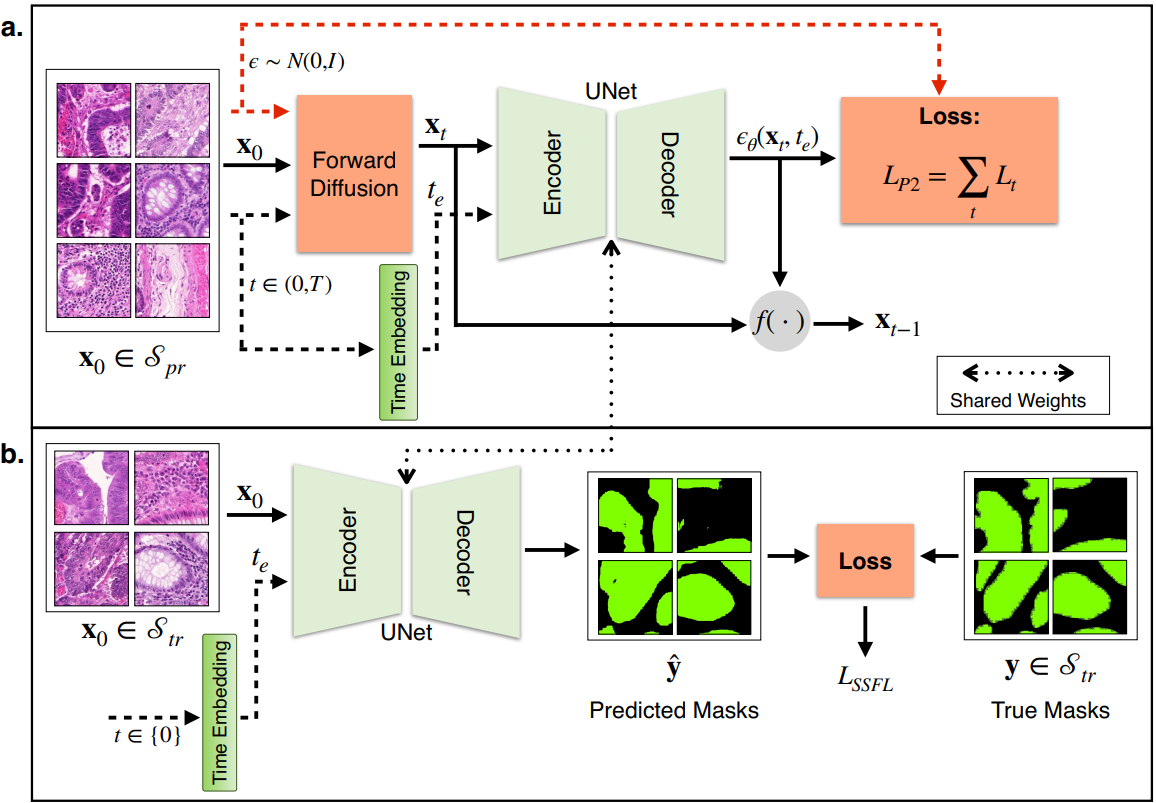
Figure 1: An overview of the proposed framework. (a) Self-supervised pre-training using diffusion: The UNet model (encoder-decoder) takes the corrupted version $\mathbf{x}_{t}$ of the image $\mathbf{x}_{0}$ and the corresponding time embedding $t_{e}$ as the input to predict the noise that takes $\mathbf{x}_{0}$ to $\mathbf{x}_{t}$, using P2 weighted [55] loss function. $f(\cdot)$ denotes the function that recovers $\mathbf{x}_{t-1}$ from $\mathbf{x}_{t}$. (b) Downstream segmentation: The self-supervised pre-trained UNet is fine-tuned end-to-end in a supervised manner to predict the segmentation masks.

Our focus is mainly on learning effective visual representations using diffusion in a self-supervised manner. This can be achieved by focusing more on the content and avoiding insignificant or trivial details of the image. But, the simple diffusion loss or variational bound in (III-B) does not guarantee much because of uniform weighting for all the time steps. Choi et al. [55] proposed a perception prioritized (P2) weighting and demonstrated that P2 weighting provides a good inductive bias for learning rich visual concepts by boosting weights at the coarse and the content stage and suppressing the weights at the clean-up stage (say high SNR or initial time steps). The variational bound with the P2 weighting scheme is

$$L_{\text{P2}} =\sum_{t\geq 1}L_{t},$$

$$L_{t} =\underset{\mathbf{x}_{0},\epsilon}{{\mathbb{E}}}\Bigr{[}\frac{1}{(k+\text{SNR}(t))^{\gamma}}\|\epsilon-\epsilon_{\boldsymbol{\theta}}(\mathbf{x}_{t},t)\|^{2}\Bigr{]},$$ (7)

where $\gamma$ is a hyperparameter that controls the strength of down-weighting focus on learning imperceptible details (high SNR). Here, $k$ is also a hyperparameter that prevents exploding weights for extremely small SNRs and determines the sharpness of the weighting scheme. SNR of the noisy sample $\mathbf{x}_{t}$ is obtained by taking the ratio of the squares of coefficients of $\mathbf{x}_{0}$ and $\epsilon$, corresponding to signal and noise variances respectively. i.e. $\text{SNR}(t)=\frac{\bar{\alpha}_{t}}{1-\bar{\alpha}_{t}}$.

We finally use the P2 weighting loss (III-B) for the DDPM training (Hyper-parameter details described later). It is to be noted that, architecturally, DDPM solves a regression task using a UNet-like base network, which takes the noisy image (along with the time embedding) as the input to predict the noise content as shown in Fig. 1(a). We use all the available unannotated images from the set $\mathcal{S}_{\text{pr}}$ to train the network in a self-supervised manner to obtain a rich set of representations $f_{\theta}$ for the input data distribution. Note that our objective of training a DDPM is not data generation but self-supervised representation learning.
Post-training, we propose to use the exact same base UNet (obtained via DDPM training) to fine-tune for the downstream H&E stained histopathological image segmentation tasks Fig. 1(b). The timestamp is added as an embedding layer with $t\in\{0\}$ since the downstream task does not involve or require noisy predictions. In other words, $\mathbf{x}_{0}$ is enough without any need for the noisy versions $\mathbf{x}_{1},\mathbf{x}_{2},\dots,\mathbf{x}_{T}$. The segmentation network is then trained using a multi-loss function proposed in the next section.

III-C Segmentation via Multi-Loss Formulation

In histopathology, segmentation is majorly based on the structural aspects of the underlying images. Further, on many occasions, class imbalance is also inevitable because of patch-based analysis, which often introduces class dominance. Hence we propose a multi-loss function which is a combination of structural similarity (SS) loss [56] and focal loss (FL), which simultaneously caters to preserving structural importance and mitigating class imbalance.

III-C1 Structural Similarity Loss

Structural similarity (SS) loss is designed to achieve a high positive linear correlation between the ground truth and the predicted segmentation masks. Zhao et al. [56] proposed it as a reweighted version of cross-entropy loss. However, we modify it as the weighted absolute error between ground truth and predicted segmentation masks with the weights being the cross-entropy loss as

$$\mathcal{L}_{SS}(y_{nc},\hat{y}_{nc}) =\mathcal{L}_{CE}\cdot f_{nc}\cdot e_{nc},$$

$$e_{nc} =\Big{|}\frac{y_{nc}-\mu_{y_{nc}}+C_{1}}{\sigma_{y_{nc}}+C_{1}}-\frac{\hat{y}_{nc}-\mu_{\hat{y}_{nc}}+C_{1}}{\sigma_{\hat{y}_{nc}}+C_{1}}\Big{|},$$

$$f_{nc} =\mathbf{1}_{\{e_{nc}>\beta e_{{max}}\}},\text{ and }$$

$$\mathcal{L}_{CE} =-\frac{1}{{N}}\sum_{n=0}^{{N}-1}\sum_{c=0}^{{C}-1}y_{nc}\ log\ \hat{y}_{nc},$$ (8)

where $\mu_{y_{nc}}$ and $\sigma_{y_{nc}}$ are the mean and standard deviation of the ground truth $y_{nc}$ respectively. $n$ and $c$ correspond to batch $N$ and channels $C$ respectively. $\hat{y}$ is the predicted segmentation mask and $C_{1}=0.01$ is an empirically set stability factor. The absolute error $e_{nc}$ measures the degree of linear correlation between two image patches. $e_{\text{max}}$ is the maximum value of $e_{nc}$, $\beta\in[0,1)$ is a weight factor with $\beta=0.1$ in practice, $\mathbf{1_{\{.\}}}$ is the indicator function, and $\mathcal{L}_{CE}$ is the cross-entropy loss. The structural similarity loss is expressed as

$$\mathcal{L}_{SS}=\frac{1}{M}\sum_{n=0}^{{N}-1}\sum_{c=0}^{{C}-1}\mathcal{L}_{SS}(y_{nc},\hat{y}_{nc})$$ (9)

where $M=\sum_{n=0}^{{N}-1}\sum_{c=0}^{{C}-1}f_{nc}$ is the number of hard examples. $f_{nc}$ is used to consider the pixels with the significant absolute error between the predicted and ground truth segmentation masks for every class, and $\mathcal{L}_{CE}$ adds weighting to those pixels. Here, $\mathcal{L}_{CE}$ is the dynamic weighting factor varying over the iterations based on the prediction. We empirically observe the effect of this modified structural similarity loss in boosting the segmentation performance in Sec. IV-F2.

III-C2 Focal Loss

Focal loss is shown to perform well in the presence of imbalanced datasets [57], defined as:

$$\mathcal{L}_{FL}=-\frac{1}{{N}}\sum_{n=0}^{{N}-1}\sum_{c=0}^{{C}-1}(1-\hat{y}_{nc})^{\gamma}y_{nc}log\hat{y}_{nc},$$ (10)

where N denotes the batch size, C denotes the number of classes, and $y_{nc}$, $\hat{y}_{nc}$ are the ground truth and predicted values for any pixel corresponding to a class. $(1-\hat{y}_{nc})^{\gamma}$ acts as a weighting factor and takes care of the class imbalance. The value of $\gamma$ is set to $2.0$ empirically. The final loss function for supervised fine-tuning our method is a weighted combination of the structural similarity and the focal loss given by $\mathcal{L}_{SSFL}=\mathcal{L}_{SS}+\lambda\mathcal{L}_{FL}$, where $\lambda$ is a hyperparameter.

IV Experiments and Results

IV-A Datasets

For our experiments, we use three datasets namely the Head and Neck Cancer Dataset, Gland segmentation in colon histology images (GlaS), and (multi-organ nucleus segmentation (MoNuSeg). The details of the datasets used are shown in Table I. While the latter two are publically available, the former is curated, annotated, and proposed by us for research community usage. The dataset will be made available for research use upon request.

IV-A1 Head and Neck Cancer Dataset

This dataset was collected with the approval of the institutional ethical committee of All India Institute of Medical Sciences (AIIMS), New Delhi, with the approval number bearing IEC-58/04.01.2019.

A total of $163$ cases of head and neck squamous cell carcinoma (SCC) [58] were retrieved from the Department of Pathology of AIIMS archives. Tumor tissue had been fixed in 10% neutral buffered formalin, routinely processed, and embedded into paraffin blocks. Representative H&E stained sections lacking cutting artifacts were selected. Images were captured at 10x magnification using a digital camera attached to a microscope. A minimum of four images were obtained from each case. A team of trained pathologists performed manual annotation of the captured images. Images were annotated using an online image annotation tool into three classes: malignant, non-malignant stroma, and non-malignant epithelium. All SCC tumor cell islands were marked as malignant. Non-malignant stroma included fibro-collagenous and adipose tissue and skeletal muscle. Non-malignant epithelium included all benign squamous epithelium adjacent to the tumor or from resection margins. All the tissue present in an image was annotated. Diagnosis of cancer requires distinction of cancer areas from the non-malignant epithelium and demonstration of invasion by cancer into the non-malignant stroma. Thus, delineating the three classes would aid a pathologist in identifying invasion by cancer cells. We use images from confirmed cases of cancers that have been surgically removed completely, and there is no ambiguity in the diagnosis, as we have ample tissue to study under the microscope. There are $1584$ images in the collected dataset, of which $507$ are annotated.

IV-A2 Public Datasets

We analyze two publicly available datasets: GlaS [59] and MoNuSeg [60]. GlaS contains $165$ images from $16$ H&E stained sections of stage T3/T4 colorectal adenocarcinoma, showing notable inter-subject variability in stain distribution and tissue architecture. Images are mostly $775\times 522$ in resolution. $85$ images are for training and $80$ for testing. We use the training set for self-supervised pre-training and split the $80$ test images into train-test sets for segmentation. $52$ visual fields from malignant and benign regions were selected for diverse tissue architectures. Pathologists annotated glandular boundaries, categorizing regions into malignant and benign classes.

The MoNuSeg dataset consists of H&E stained images at 40x magnification. For nuclear appearance diversity, one image per patient was chosen and cropped into 1000 × 1000 sub-images dense in nuclei. Annotated classes cover epithelial and stromal nuclei, resolving overlaps in classes by assigning pixels to the largest nucleus. This dataset contains $37$ training and $14$ testing images. Initially, three classes are annotated: nucleus boundary, within-nucleus (foreground), and outside-nuclei (background). However, our study combines the nucleus boundary and nucleus into one class. Our pre-training stage involves all $37$ training images, while the remaining 14 are used for segmentation. Sample images from all the evaluation datasets are shown in Fig. 2.

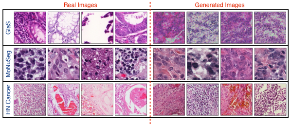
Figure 2: Sample real and generated patches using diffusion on three datasets: GlaS [60], MoNuSeg [59], and HN cancer (ours). The first four images in each row represent real image patches, and the last four images represent the generated image patches.

The GlaS and MoNuSeg datasets use fixed training and testing sets. The training set images serve as unlabeled data for self-supervised pre-training, while the testing set images provide labeled data for segmentation. This guarantees that pre-training and fine-tuning stages use mutually exclusive image sets. Labeled images are further divided into train and test subsets, with the latter used only for performance assessment. The HN cancer dataset also comprises separate labeled and unlabeled images. Patches of 256 × 256 (stride of 64 for GlaS and MoNuSeg, 256 for HN cancer) are extracted for training and evaluation. Dataset details are in Table VI.

TABLE I: Number of Images and Patches in Each Dataset. The Numbers in Brackets (in red) Indicate the Patches.

Dataset	Unlabeled Images	Labeled Images
		Train	Test
GlaS	85 (3681)	64 (2685)	16 (720)
MoNuSeg	37 (5328)	11 (1584)	3 (432)
HN cancer	1057 (21140)	404 (8080)	101 (2020)

TABLE II: Performance Evaluation of the Proposed Method and Baseline Methods on GlaS, MoNuSeg, and HN Cancer Datasets.

	GlaS				MoNuSeg				HN Cancer
Method	Accuracy	Precision	Recall	F1-Score	Accuracy	Precision	Recall	F1-Score	Accuracy	Precision	Recall	F1-Score
UNet [5]	0.8979	0.8564	0.8897	0.8521	0.8931	0.8536	0.8343	0.8411	0.8664	0.7976	0.8709	0.7325
Attention UNet [61]	0.9080	0.8924	0.8805	0.8712	0.8988	0.8663	0.8412	0.8498	0.9078	0.8778	0.8840	0.8098
VAE [25]	0.8975	0.8649	0.8676	0.8400	0.8923	0.8584	0.8325	0.8386	0.8927	0.8674	0.8766	0.7894
Context Restoration [11]	0.9236	0.9051	0.8980	0.8902	0.9021	0.8742	0.8440	0.8533	0.9124	0.9038	0.8692	0.8175
Contrastive [51]	0.9014	0.8747	0.8837	0.8565	0.8939	0.8671	0.8282	0.8392	0.8917	0.8895	0.8548	0.7858
CS-CO [52]	0.9165	0.8864	0.8956	0.8790	0.8737	0.8326	0.7915	0.8068	0.9108	0.8409	0.8786	0.7811
DIM [62]	0.9217	0.8995	0.8989	0.8805	0.8967	0.8542	0.8520	0.8498	0.9062	0.8836	0.8820	0.8097
Inpainting [15]	0.9043	0.8951	0.8776	0.8658	0.8947	0.8704	0.8304	0.8400	0.8872	0.8895	0.8536	0.7843
Ours	0.9381	0.9236	0.9147	0.9108	0.9096	0.8844	0.8550	0.8651	0.9265	0.8933	0.9050	0.8424

TABLE III: Mean and Standard Deviation values on the Three Datasets GlaS, MoNuSeg, and HN Cancer for All the Metrics.

Dataset	Accuracy	Precision	Recall	F1-score
GlaS	0.9373 $\pm$ 0.0006	0.9211 $\pm$ 0.0019	0.9137 $\pm$ 0.0008	0.9089 $\pm$ 0.0013
MoNuSeg	0.9073 $\pm$ 0.0016	0.8818 $\pm$ 0.0023	0.8513 $\pm$ 0.0041	0.8612 $\pm$ 0.0030
HN cancer	0.9256 $\pm$ 0.0013	0.8948 $\pm$ 0.0043	0.8998 $\pm$ 0.0046	0.8382 $\pm$ 0.0035

IV-B Baselines for Comparison

We compare our framework with two fully supervised benchmarks: (a) UNet[5] - a standard model for medical image segmentation, and (b) Attention UNet[61] with Random initialization - a UNet incorporating an attention mechanism designed for CT abdominal image segmentation. The remaining baselines adopt diverse pretext tasks for self-supervision:(1) VAE [25]: A UNet-based variational autoencoder pre-trained and down streamed for segmentation. (2) Context Restoration [11]: Self-supervised learning through context restoration, targeted at medical image analysis. (3) Contrastive Learning [51]: Leveraging self-supervised contrastive learning for acquiring image representations. (4) CS-CO [52]: A histopathological image-specific contrastive learning technique utilizing novel image augmentations. (5) Deep InfoMax (DIM) [62]: Unsupervised representation learning by maximizing mutual information between input and output. (6) Inpainting [15]: UNet model trained using image inpainting as a pretext task. All methods are trained until loss convergence, followed by fine-tuning for segmentation.

IV-C Implementation Details

We use the attention-based UNet as the encoder-decoder network for pre-training and fine-tuning. The time stamps are drawn uniformly randomly between $0$ and $T$ and then input to the corresponding embedding layer for the network during pre-training. We train the network for $100$ epochs with a learning rate of $0.0001$ using Adam optimizer and a batch size of $8$. For the downstream segmentation, we initialize the UNet, except for the last few layers, with the pre-trained weights of the pretext task and then fine-tune the entire network end-to-end with the Adam optimizer for $150$ epochs. The batch size is $8$, and the learning rate is $0.0001$. The multi-loss function’s regularization scaling parameter $\lambda$ is set to $1.0$. We use random horizontal and vertical flips, color jittering, and Gaussian blur as augmentations. All the comparisons are with UNet-based networks except for CS-CO, a Resnet-based network. The hyperparameters are kept the same across all the methods for fair comparison. We use accuracy, precision, sensitivity (recall), and F1-score as the evaluation metrics for our segmentation task.

IV-D Quantitative and Qualitative Results

We demonstrate the effect of self-supervision tasks by transferring the learned representations to the histopathological image segmentation task. Here, we compare our proposed diffusion-based self-supervision against other existing self-supervision tasks like context restoration [11], contrastive learning [51], and CS-CO [52]. The self-supervised approaches [51], [52] are pathology specific, whereas [11] is pathology agnostic but still related to medical image analysis. We also train a network with random initialization, which we use as our baseline method. Moreover, we compare our approach with various methods as described in Section IV-B. Our method shares certain similarities with [28, 63, 64], but these methods are mainly focused on generating high-quality images and learning good representations but are not tuned specifically for segmentation.

TABLE IV: Generation Performance (FID Scores) of Self-Supervised Pre-Training on Three Datasets: GlaS, MoNuSeg, and HN Cancer and the Combination of all Datasets.

Dataset	GlaS	MoNuSeg	HN cancer	Combined
FID Score	82.44	15.32	6.80	7.63

Fig. 2 shows examples of generated images from learning the self-supervised pretext task using diffusion. The generation performance of the diffusion model is captured using a popular metric, Frechet Inception Distance (FID) [65], which is measured between images from a dataset and a set of generated images. We use $1000$ images from each dataset and generated images to compute FID scores, which are shown in Table IV. One can observe that the FID scores are lower when the datasets contain more samples, indicating that the generation performance increases with the number of training patches. This can also be qualitatively understood in Fig. 2, where the generated images of GlaS, containing lower unlabeled images (see Table. I), are noisy. Moreover, we note that good generation performance also translates to better segmentation performance on all datasets.

Our approach achieves superior segmentation performance over other self-supervised methods on all the metrics for GlaS and MoNuSeg datasets and three metrics except precision on the HN cancer dataset. Table II shows the evaluation performance of all methods on all three segmentation datasets. We observe an improvement of at least $2$ % for GlaS, $1-1.5$ % for MoNuSeg, and $2-2.5$ % HN cancer datasets with respect to F1-score. Encouraging results are that the margin in recall (sensitivity) is better compared to precision in boosting the F1 score, particularly for the HN cancer dataset. Moreover, we also include performances of our approach on all three datasets over multiple runs (weight initialization) in Table III to demonstrate the stability in training the segmentation models. Finally, Fig. 3 clearly demonstrates the superior qualitative performance (In comparison to the ground truth) of the proposed method over other self-supervised methods on all three datasets.

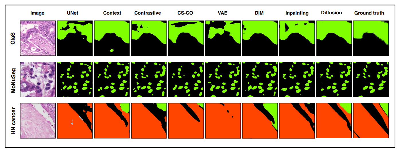
Figure 3: Qualitative Results of the proposed method (diffusion) along with other methods: UNet [5], Context Restoration [11], Contrastive learning [51], CS-CO [52], VAE [25], DIM [62], Inpainting [15], and Diffusion (ours).

TABLE V: Effect of Varying the Number of Time Stamps on Downstream Segmentation Performance using F1-score on GlaS and MoNuSeg Datasets.

Time stamps	GlaS	MoNuSeg
10	0.9009	0.8541
50	0.9094	0.8587
100	0.9075	0.8577
250	0.9086	0.8614
500	0.9030	0.8546
1000	0.9108	0.8651
2000	0.9079	0.8576
5000	0.9017	0.8556

IV-E Cross-Dataset Segmentation

Table I shows that the HN cancer dataset contains the most unannotated images, followed by MoNuSeg and GLaS. From Fig. 2, it can be seen that GLaS and HN cancer datasets have comparable mask sizes for any class in the annotated segmentation maps, whereas the mask size (corresponding to the nucleus class) is small. This indicates some amount of correlation between the two datasets.

Hence, from Table VII, we observe that the segmentation performance on the GLaS dataset using a model pre-trained on the HN dataset is good. However, self-supervision using the GLaS dataset and segmentation on the HN dataset doesn’t follow the same pattern due to the low number of unannotated images in the GLaS dataset. The model achieves good performance on the MoNuSeg dataset when pre-trained and fine-tuned on MoNuSeg itself. This indicates that a certain degree of similarity between datasets aids in learning task-agnostic visual representations using diffusion-based self-supervision.

We also pre-train the diffusion model using a combination of unannotated images from all three datasets and then learn separate segmentation models for each dataset. From Table VI, we notice a performance boost on all the datasets, validating that the performance of downstream tasks can be enhanced by learning more generalizable representations from diverse data distributions.

TABLE VI: Evaluation of Performance of Combining the Three Datasets GlaS, MoNuSeg, and HN Cancer During Self-Supervision.

Metric	GlaS	MoNuSeg	HN cancer
Accuracy	0.9397	0.9113	0.9245
Precision	0.9232	0.8856	0.8872
Recall	0.9154	0.8571	0.9039
F1-score	0.9126	0.8676	0.8357

IV-F Ablations

IV-F1 Effect of Diffusion Time Steps

We observe the effect of varying the number of time steps $T$ in the diffusion process during the pre-training stage on the performance of segmentation. The time steps are varied from $50$ to $5000$. Table V shows the F1 scores on MoNuSeg and GlaS datasets. We notice that the performance degrades when $T$ is either too high or too low for both datasets. When $T$ is high, the noise addition in the later steps is a very slow process and less significant. As a result, most noising steps are high SNR processes, making the network learn many imperceptible details and content from these images. Hence, a performance drop is expected. On the other hand, when $T$ is very low, the noise addition happens very fast, adding significant noise in each step. This causes the noising process to operate in a low SNR regime, making the model learn predominantly coarse details over content information, resulting in a performance drop [55]. Hence, a trade-off exists based on the choice of $T$, impacting the segmentation performance. We observe that the F1 scores roughly peak at $T=1000$ for both datasets, which we fix for pre-training our model.

TABLE VII: Evaluation of Segmentation Performance using F1-score on Cross-Dataset Self-Supervision. Row Indicates the Pre-trained Dataset.

Dataset	GlaS	MoNuSeg	HN cancer
GlaS	0.9108	0.8620	0.8037
MoNuSeg	0.8849	0.8651	0.8072
HN cancer	0.9124	0.8596	0.8424

IV-F2 Effect of Loss Functions:

In our work, we use a combination of structural similarity and focal losses. In Table VIII, we explore the contribution of individual losses: cross-entropy (CE), SS, and FL. We observe that CE loss performs well only on MoNuSeg, where the training data is less, and poorly on the other two datasets. Qualitative results are presented in Fig. 4 to show the effect of different loss functions on segmentation performance. When we have access to more training data, both SS and FL perform better individually. Finally, the combination of SS and FL gives the best performance on all the segmentation datasets.

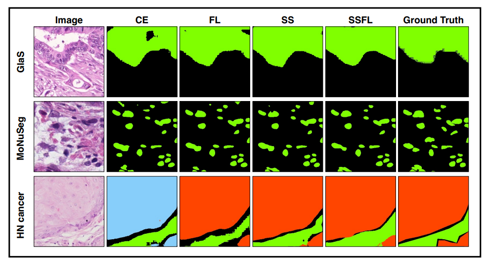
Figure 4: Qualitative Results of the proposed multi-loss function on all three datasets. The losses are abbreviated as CE - cross-entropy, FL - focal loss, and SS - structural similarity.

TABLE VIII: Effect of Multi Loss Function on All Three Datasets. CE, SS, and FL Indicate Cross Entropy, Structural Similarity, and Focal Losses, Respectively. F1-score is Used for the Comparison Here.

Loss	GlaS	MoNuSeg	HN cancer
CE	0.8792	0.8641	0.8086
SS	0.8858	0.8558	0.8308
FL	0.8859	0.8633	0.8091
SS + FL	0.9108	0.8651	0.8424

IV-F3 Effect of Loss Scaling Factor

In order to evaluate the contribution of each loss term in our multi-loss function, we vary the hyperparameter $\lambda\in\{0.1,0.5,1,10\}$. From Table IX, we observe that an equal weighting of both the SS loss and focal loss ($\lambda=1$) offers the best performance in terms of F1 scores, indicating that a balancing reconstruction error and class imbalance is necessary for efficient learning.

TABLE IX: Evaluation of Segmentation Performance using F1-score on Varying Scale Factor of the Multi Loss Function.

Scale factor	GlaS	MoNuSeg	HN cancer
0.1	0.9089	0.8645	0.8255
0.5	0.9081	0.8605	0.8200
1.0	0.9108	0.8651	0.8424
10	0.9077	0.8627	0.8164

IV-F4 Effect of Varying Architecture Size

We experiment with varying UNet block sizes and record the effect of network size on the segmentation performance. The number of downsampling (or upsampling) levels is varied between $3$ to $5$, along with the number of output channels in each of the levels in the UNet architecture. Table X illustrates the number of levels accompanied by the number of output channels in each level. It is observed that a UNet consisting of $4$ levels with $(64,128,256,512)$ output channels performs the best. Moreover, within $4$ level UNet architectures, we note that the standard UNet architecture performs the best, indicating that this network efficiently trades off bias and overfitting.

TABLE X: Segmentation Performance for Different Sizes of UNet Architecture. F1-score is Used as the Evaluation Metric Here. The Numbers in Brackets Indicate the Channels.

Blocks	GlaS	MoNuSeg
3 (64, 128, 256)	0.9012	0.8580
4 (32, 64, 128, 256)	0.9001	0.8603
4 (64, 128, 192, 256)	0.9073	0.8610
4 (64, 128, 256, 512)	0.9108	0.8651
5 (64, 128, 256, 512, 1024)	0.8937	0.8556

V Conclusion and Discussion

In this work, We proposed a novel two-stage learning approach for segmenting histopathological images. The first stage consists of learning good visual representations of histopathological images through self-supervised learning. This is achieved through a diffusion model trained without annotated data. Since segmentation is an image-to-image task, it benefits from learning representations through image-to-image self-supervision. It is noteworthy that the quality of representations has a direct impact on the performance of downstream tasks such as classification and segmentation. Hence, the self-supervised pre-training stage learns good representations that can later be downstream to any task in general. Moreover, since datasets generally contain low amounts of annotated images, SSL methods can perform better through the use of an abundant number of unannotated images. Once the pre-training is complete, we fine-tune the UNet model for segmenting histopathological images using a novel multi-loss function composed of structural similarity loss and focal loss.

We also introduce a new head and neck cancer dataset consisting of annotated and unannotated histopathological images. The research community can use this dataset to develop unsupervised, self-supervised, and even fully supervised machine learning algorithms to analyze and understand histopathological images for segmentation, detection, classification, and many other tasks.

The results presented in Section IV give us some interesting insights into the problem. Firstly, it can be seen that the generation performance of the DDPM impacts the learning of effective representations. Secondly, task-specific loss functions need to be carefully designed so that models are able to leverage task-relevant information during optimization. In summary, our approach serves as a stepping stone for exploring generative self-supervised training as a pretext task for learning-based medical applications.

References

- [1] C. Lu, M. Mahmood, N. Jha, and M. Mandal, “Automated segmentation of the melanocytes in skin histopathological images,” IEEE journal of biomedical and health informatics, vol. 17, no. 2, pp. 284–296, 2013.
- [2] ——, “A robust automatic nuclei segmentation technique for quantitative histopathological image analysis,” Analytical and Quantitative Cytology and Histology, vol. 34, pp. 296–308, 2012.
- [3] M. Mete, X. Xu, C.-Y. Fan, and G. Shafirstein, “Automatic delineation of malignancy in histopathological head and neck slides,” in BMC bioinformatics, vol. 8, no. 7. BioMed Central, 2007, pp. 1–13.
- [4] M. Springenberg, A. Frommholz, M. Wenzel, E. Weicken, J. Ma, and N. Strodthoff, “From modern cnns to vision transformers: Assessing the performance, robustness, and classification strategies of deep learning models in histopathology,” Medical Image Analysis, vol. 87, p. 102809, 2023.
- [5] O. Ronneberger, P. Fischer, and T. Brox, “U-net: Convolutional networks for biomedical image segmentation,” in Medical Image Computing and Computer-Assisted Intervention – MICCAI 2015. Springer Intl. Publishing, 2015, pp. 234–241.
- [6] A. Albayrak and G. Bilgin, “A hybrid method of superpixel segmentation algorithm and deep learning method in histopathological image segmentation,” in 2018 Innovations in Intelligent Systems and Applications (INISTA). IEEE, 2018, pp. 1–5.
- [7] Y. Xu, Z. Jia, L.-B. Wang, Y. Ai, F. Zhang, M. Lai, E. I. Chang et al., “Large scale tissue histopathology image classification, segmentation, and visualization via deep convolutional activation features,” BMC bioinformatics, vol. 18, no. 1, pp. 1–17, 2017.
- [8] J. Xu, “A review of self-supervised learning methods in the field of medical image analysis,” Intl. Journal of Image, Graphics and Signal Processing (IJIGSP), vol. 13, no. 4, pp. 33–46, 2021.
- [9] R. Krishnan, P. Rajpurkar, and E. J. Topol, “Self-supervised learning in medicine and healthcare,” Nature Biomedical Engineering, vol. 6, no. 12, pp. 1346–1352, 2022.
- [10] R. Zhang, P. Isola, and A. A. Efros, “Split-brain autoencoders: Unsupervised learning by cross-channel prediction,” in 2017 IEEE Conf. on Computer Vision and Pattern Recognition (CVPR), 2017, pp. 645–654.
- [11] L. Chen, P. Bentley, K. Mori, K. Misawa, M. Fujiwara, and D. Rueckert, “Self-supervised learning for medical image analysis using image context restoration,” Medical Image Analysis, vol. 58, p. 101539, 2019.
- [12] S. Gidaris, P. Singh, and N. Komodakis, “Unsupervised representation learning by predicting image rotations,” in Intl. Conf. on Learning Representations, 2018.
- [13] R. Zhang, P. Isola, and A. A. Efros, “Colorful image colorization,” in Computer Vision – ECCV 2016. Springer Intl. Publishing, 2016, pp. 649–666.
- [14] C. Ledig, L. Theis, F. Huszár, J. Caballero, A. Cunningham, A. Acosta, A. Aitken, A. Tejani, J. Totz, Z. Wang, and W. Shi, “Photo-realistic single image super-resolution using a generative adversarial network,” in 2017 IEEE Conf. on Computer Vision and Pattern Recognition (CVPR), 2017, pp. 105–114.
- [15] D. Pathak, P. Krahenbuhl, J. Donahue, T. Darrell, and A. A. Efros, “Context encoders: Feature learning by inpainting,” in 2016 IEEE Conf. on Computer Vision and Pattern Recognition (CVPR). Los Alamitos, CA, USA: IEEE Computer Society, jun 2016, pp. 2536–2544.
- [16] C. L. Srinidhi, S. W. Kim, F.-D. Chen, and A. L. Martel, “Self-supervised driven consistency training for annotation efficient histopathology image analysis,” Medical Image Analysis, vol. 75, p. 102256, 2022.
- [17] P. Chhipa, R. Upadhyay, G. Pihlgren, R. Saini, S. Uchida, and M. Liwicki, “Magnification prior: A self-supervised method for learning representations on breast cancer histopathological images,” in 2023 IEEE/CVF Winter Conf. on Applications of Computer Vision (WACV). Los Alamitos, CA, USA: IEEE Computer Society, jan 2023, pp. 2716–2726.
- [18] J. Xu, J. Hou, Y. Zhang, R. Feng, C. Ruan, T. Zhang, and W. Fan, “Data-efficient histopathology image analysis with deformation representation learning,” in 2020 IEEE Intl. Conf. on Bioinformatics and Biomedicine (BIBM), 2020, pp. 857–864.
- [19] X. Wang, S. Yang, J. Zhang, M. Wang, J. Zhang, J. Huang, W. Yang, and X. Han, “Transpath: Transformer-based self-supervised learning for histopathological image classification,” in Medical Image Computing and Computer Assisted Intervention – MICCAI 2021. Springer Intl. Publishing, 2021, pp. 186–195.
- [20] C. Abbet, I. Zlobec, B. Bozorgtabar, and J.-P. Thiran, “Divide-and-rule: Self-supervised learning for survival analysis in colorectal cancer,” in Medical Image Computing and Computer Assisted Intervention – MICCAI 2020. Cham: Springer Intl. Publishing, 2020, pp. 480–489.
- [21] D. Mahapatra, B. Bozorgtabar, J.-P. Thiran, and L. Shao, “Structure preserving stain normalization of histopathology images using self supervised semantic guidance,” in Medical Image Computing and Computer Assisted Intervention – MICCAI 2020. Springer Intl. Publishing, 2020, pp. 309–319.
- [22] A. C. Quiros, R. Murray-Smith, and K. Yuan, “Pathologygan: Learning deep representations of cancer tissue,” Machine Learning for Biomedical Imaging, vol. 1, pp. 1–47, 2021.
- [23] A. Claudio Quiros, N. Coudray, A. Yeaton, W. Sunhem, R. Murray-Smith, A. Tsirigos, and K. Yuan, “Adversarial learning of cancer tissue representations,” in Medical Image Computing and Computer Assisted Intervention – MICCAI 2021. Cham: Springer Intl. Publishing, 2021, pp. 602–612.
- [24] Y. Zhao, F. Yang, Y. Fang, H. Liu, N. Zhou, J. Zhang, J. Sun, S. Yang, B. Menze, X. Fan, and J. Yao, “Predicting lymph node metastasis using histopathological images based on multiple instance learning with deep graph convolution,” in 2020 IEEE/CVF Conf. on Computer Vision and Pattern Recognition (CVPR), 2020, pp. 4836–4845.
- [25] D. P. Kingma and M. Welling, “Auto-Encoding Variational Bayes,” in 2nd Intl. Conf. on Learning Representations, ICLR 2014, Banff, AB, Canada, April 14-16, 2014, Conference Track Proceedings, 2014.
- [26] I. Goodfellow, J. Pouget-Abadie, M. Mirza, B. Xu, D. Warde-Farley, S. Ozair, A. Courville, and Y. Bengio, “Generative adversarial nets,” in Advances in Neural Information Processing Systems, Z. Ghahramani, M. Welling, C. Cortes, N. Lawrence, and K. Weinberger, Eds., vol. 27. Curran Associates, Inc., 2014.
- [27] K. Zhang, “On mode collapse in generative adversarial networks,” in Artificial Neural Networks and Machine Learning–ICANN 2021: 30th Intl. Conf. on Artificial Neural Networks, Bratislava, Slovakia, September 14–17, 2021, Proceedings, Part II 30. Springer, 2021, pp. 563–574.
- [28] J. Ho, A. Jain, and P. Abbeel, “Denoising diffusion probabilistic models,” Advances in neural information processing systems, vol. 33, pp. 6840–6851, 2020.
- [29] P. Dhariwal and A. Q. Nichol, “Diffusion models beat GANs on image synthesis,” in Advances in Neural Information Processing Systems, 2021.
- [30] J. Wu, R. FU, H. Fang, Y. Zhang, Y. Yang, H. Xiong, H. Liu, and Y. Xu, “Medsegdiff: Medical image segmentation with diffusion probabilistic model,” in Medical Imaging with Deep Learning, 2023.
- [31] J. Wu, R. Fu, H. Fang, Y. Zhang, and Y. Xu, “Medsegdiff-v2: Diffusion based medical image segmentation with transformer,” ArXiv, vol. abs/2301.11798, 2023.
- [32] C. L. Srinidhi, O. Ciga, and A. L. Martel, “Deep neural network models for computational histopathology: A survey,” Medical Image Analysis, vol. 67, p. 101813, 2021.
- [33] D. Komura and S. Ishikawa, “Machine learning methods for histopathological image analysis,” Computational and Structural Biotechnology Journal, vol. 16, pp. 34–42, 2018.
- [34] Z. Zhou, M. M. R. Siddiquee, N. Tajbakhsh, and J. Liang, “Unet++: Redesigning skip connections to exploit multiscale features in image segmentation,” IEEE Transactions on Medical Imaging, vol. 39, no. 6, pp. 1856–1867, 2020.
- [35] K. He, X. Zhang, S. Ren, and J. Sun, “Deep residual learning for image recognition,” in 2016 IEEE Conf. on Computer Vision and Pattern Recognition (CVPR), 2016, pp. 770–778.
- [36] Y. Xu, J.-Y. Zhu, E. I.-C. Chang, M. Lai, and Z. Tu, “Weakly supervised histopathology cancer image segmentation and classification,” Medical Image Analysis, vol. 18, no. 3, pp. 591–604, 2014.
- [37] H. Chen, X. Qi, L. Yu, and P.-A. Heng, “Dcan: Deep contour-aware networks for accurate gland segmentation,” in 2016 IEEE Conf. on Computer Vision and Pattern Recognition (CVPR), 2016, pp. 2487–2496.
- [38] Y. Liu, Q. He, H. Duan, H. Shi, A. Han, and Y. He, “Using sparse patch annotation for tumor segmentation in histopathological images,” Sensors, vol. 22, no. 16, 2022.
- [39] J. Bokhorst, H. Pinckaers, P. van Zwam, I. Nagtegaal, J. van der Laak, and F. Ciompi, “Learning from sparsely annotated data for semantic segmentation in histopathology images,” in Proc. of The 2nd Intl. Conf. on Medical Imaging with Deep Learning, vol. 102. PMLR, 2019, pp. 84–91.
- [40] J. Yan, H. Chen, X. Li, and J. Yao, “Deep contrastive learning based tissue clustering for annotation-free histopathology image analysis,” Computerized Medical Imaging and Graphics, vol. 97, p. 102053, 2022.
- [41] P. Yang, Y. Zhai, L. Li, H. Lv, J. Wang, C. Zhu, and R. Jiang, “A deep metric learning approach for histopathological image retrieval,” Methods, vol. 179, pp. 14–25, 2020, interpretable machine learning in bioinformatics.
- [42] M. N. Gurcan, L. E. Boucheron, A. Can, A. Madabhushi, N. M. Rajpoot, and B. Yener, “Histopathological image analysis: A review,” IEEE Reviews in Biomedical Engineering, vol. 2, pp. 147–171, 2009.
- [43] L. Qu, S. Liu, X. Liu, M. Wang, and Z. Song, “Towards label-efficient automatic diagnosis and analysis: a comprehensive survey of advanced deep learning-based weakly-supervised, semi-supervised and self-supervised techniques in histopathological image analysis,” Physics in Medicine & Biology, vol. 67, no. 20, p. 20TR01, oct 2022.
- [44] L. Jing and Y. Tian, “Self-supervised visual feature learning with deep neural networks: A survey,” IEEE Transactions on Pattern Analysis and Machine Intelligence, vol. 43, no. 11, pp. 4037–4058, 2021.
- [45] X. Liu, F. Zhang, Z. Hou, L. Mian, Z. Wang, J. Zhang, and J. Tang, “Self-supervised learning: Generative or contrastive,” IEEE Transactions on Knowledge and Data Engineering, vol. 35, no. 1, pp. 857–876, 2023.
- [46] N. A. Koohbanani, B. Unnikrishnan, S. A. Khurram, P. Krishnaswamy, and N. Rajpoot, “Self-path: Self-supervision for classification of pathology images with limited annotations,” IEEE Transactions on Medical Imaging, vol. 40, no. 10, pp. 2845–2856, 2021.
- [47] T. Chen, S. Kornblith, M. Norouzi, and G. Hinton, “A simple framework for contrastive learning of visual representations,” in Proceedings of the 37th Intl. Conf. on Machine Learning, ser. Proceedings of Machine Learning Research, vol. 119. PMLR, 13–18 Jul 2020, pp. 1597–1607.
- [48] K. He, H. Fan, Y. Wu, S. Xie, and R. Girshick, “Momentum contrast for unsupervised visual representation learning,” in Proceedings of the IEEE/CVF Conf. on computer vision and pattern recognition, 2020, pp. 9729–9738.
- [49] J.-B. Grill, F. Strub, F. Altché, C. Tallec, P. Richemond, E. Buchatskaya, C. Doersch, B. Avila Pires, Z. Guo, M. Gheshlaghi Azar et al., “Bootstrap your own latent-a new approach to self-supervised learning,” Advances in neural information processing systems, vol. 33, pp. 21 271–21 284, 2020.
- [50] K. Chaitanya, E. Erdil, N. Karani, and E. Konukoglu, “Contrastive learning of global and local features for medical image segmentation with limited annotations,” in Advances in Neural Information Processing Systems, H. Larochelle, M. Ranzato, R. Hadsell, M. Balcan, and H. Lin, Eds., vol. 33. Curran Associates, Inc., 2020, pp. 12 546–12 558.
- [51] O. Ciga, T. Xu, and A. L. Martel, “Self supervised contrastive learning for digital histopathology,” Machine Learning with Applications, vol. 7, p. 100198, 2022.
- [52] P. Yang, X. Yin, H. Lu, Z. Hu, X. Zhang, R. Jiang, and H. Lv, “Cs-co: A hybrid self-supervised visual representation learning method for h&e-stained histopathological images,” Medical Image Analysis, vol. 81, p. 102539, 2022.
- [53] K. Stacke, J. Unger, C. Lundström, and G. Eilertsen, “Learning representations with contrastive self-supervised learning for histopathology applications,” Machine Learning for Biomedical Imaging, vol. 1, pp. 1–33, 2022.
- [54] C. Luo, “Understanding diffusion models: A unified perspective,” ArXiv, vol. abs/2208.11970, 2022.
- [55] J. Choi, J. Lee, C. Shin, S. Kim, H. Kim, and S. Yoon, “Perception prioritized training of diffusion models,” in 2022 IEEE/CVF Conf. on Computer Vision and Pattern Recognition (CVPR), 2022, pp. 11 462–11 471.
- [56] S. Zhao, B. Wu, W. Chu, Y. Hu, and D. Cai, “Correlation maximized structural similarity loss for semantic segmentation,” ArXiv, vol. abs/1910.08711, 2019.
- [57] S. Jadon, “A survey of loss functions for semantic segmentation,” in 2020 IEEE Conf. on Computational Intelligence in Bioinformatics and Computational Biology (CIBCB), 2020, pp. 1–7.
- [58] A. J. Kimple, C. M. Welch, J. P. Zevallos, and S. N. Patel, “Oral cavity squamous cell carcinoma—an overview,” Oral Health Dent Manag, vol. 13, no. 3, pp. 877–882, 2014.
- [59] K. Sirinukunwattana, J. P. Pluim, H. Chen, X. Qi, P.-A. Heng, Y. B. Guo, L. Y. Wang, B. J. Matuszewski, E. Bruni, U. Sanchez et al., “Gland segmentation in colon histology images: The glas challenge contest,” Medical image analysis, vol. 35, pp. 489–502, 2017.
- [60] N. Kumar, R. Verma, S. Sharma, S. Bhargava, A. Vahadane, and A. Sethi, “A dataset and a technique for generalized nuclear segmentation for computational pathology,” IEEE transactions on medical imaging, vol. 36, no. 7, pp. 1550–1560, 2017.
- [61] O. Oktay, J. Schlemper, L. Le Folgoc, M. Lee, M. Heinrich, K. Misawa, K. Mori, S. McDonagh, N. Y. Hammerla, B. Kainz et al., “Attention u-net: Learning where to look for the pancreas,” in Medical Imaging with Deep Learning, 2022.
- [62] R. D. Hjelm, A. Fedorov, S. Lavoie-Marchildon, K. Grewal, P. Bachman, A. Trischler, and Y. Bengio, “Learning deep representations by mutual information estimation and maximization,” in Intl. Conf. on Learning Representations, 2018.
- [63] A. Q. Nichol and P. Dhariwal, “Improved denoising diffusion probabilistic models,” in Proceedings of the 38th Intl. Conf. on Machine Learning, ser. Proceedings of Machine Learning Research, vol. 139. PMLR, 18–24 Jul 2021, pp. 8162–8171.
- [64] P. A. Moghadam, S. Van Dalen, K. C. Martin, J. Lennerz, S. Yip, H. Farahani, and A. Bashashati, “A morphology focused diffusion probabilistic model for synthesis of histopathology images,” in 2023 IEEE/CVF Winter Conf. on Applications of Computer Vision (WACV), 2023, pp. 1999–2008.
- [65] M. Heusel, H. Ramsauer, T. Unterthiner, B. Nessler, and S. Hochreiter, “Gans trained by a two time-scale update rule converge to a local nash equilibrium,” Advances in neural information processing systems, vol. 30, 2017.