Space-Time Block Preconditioning for Incompressible
Resistive Magnetohydrodynamics

Abstract

This work develops an all-at-once space-time preconditioning approach for resistive magnetohydrodynamics (MHD), with a focus on model problems targeting fusion reactor design. We consider parallel-in-time due to the long time domains required to capture the physics of interest, as well as the complexity of the underlying system and thereby computational cost of long-time integration. To ameliorate this cost by using many processors, we thus develop a novel approach to solving the whole space-time system that is parallelizable in both space and time. We develop a space-time block preconditioning for resistive MHD, following the space-time block preconditioning concept first introduced by Danieli et al. in 2022 for incompressible flow, where an effective preconditioner for classic sequential time-stepping is extended to the space-time setting. The starting point for our derivation is the continuous Schur complement preconditioner by Cyr et al. in 2021, which we proceed to generalise in order to produce, to our knowledge, the first space-time block preconditioning approach for the challenging equations governing incompressible resistive MHD. The numerical results are promising for the model problems of island coalescence and tearing mode, with the overhead computational cost associated with space-time preconditioning versus sequential time-stepping being modest and primarily in the range of 2$\times$–5$\times$, which is low for parallel-in-time schemes in general. Additionally, the scaling results for inner (linear) and outer (nonlinear) iterations are flat in the case of fixed time-step size and only grow very slowly in the case of time-step refinement.

https://orcid.org/0000-0002-0866-2485]orcid.org/0000-0002-0866-2485

http://orcid.org/0000-0002-0283-4928]orcid.org/0000-0002-0283-4928

https://orcid.org/0000-0002-1076-9206]orcid.org/0000-0002-1076-9206

[oxforduni]organization=University of Oxford,city=Oxford, postcode=OX26GG, country=UK [lanl]organization=Los Alamos National Laboratory,city=Los Alamos, postcode=87545, state=NM, country=USA [unm]organization=University of New Mexico,city=Albuquerque, postcode=87106, state=NM, country=USA

1 Introduction

Lying at the interface between electromagnetism and fluid dynamics, Magnetohydrodynamics (MHD) is responsible for modelling the behaviour of electrically charged fluids subject to electromagnetic interactions. In our work, we consider resistive plasmas as the target application, due to the relevance this covers for our partner institution CCFE [1] in the design of a nuclear fusion reactor. The equations governing the evolution of resistive plasma allow for the topology of the magnetic field lines to change, leading to phenomena in which these break or coalesce [2]. This poses challenges in the development of fusion reactors, as during these events some matter might escape the magnetic confinement and collide with the interior walls of the vessel. Such collisions can damage walls, losing heat in the process, ultimately undermining the possibility of sustaining a reaction for long periods of time. Due to the complexity and cost associated with setting up large-scale experiments, fusion researchers rely extensively on the results from numerical simulations in guiding their design choices for properly controlling the reaction.

The system of partial differential equations (PDEs) representing resistive MHD is tightly coupled, non-symmetric, and includes nonlinearities that give rise to turbulent behaviour and spawn a range of phenomena interacting at various scales of space and time. These are all characteristics that make an approximate numerical solution particularly challenging. Nonetheless, there is great interest in developing strategies for tackling these problems effectively, as testified by the amount of research dedicated to the design of stable and efficient schemes and preconditioners for accelerating the solution of the discretised MHD system; see for example [3, 4, 5, 6, 7, 8, 9], and the work this paper primarily builds on [10]. Given the difficulties already posed by having to solve this problem in a time-stepping framework, perhaps it is not surprising that few papers have considered parallel-in-time (PinT) approaches. To our knowledge, only [11, 12, 13] and more recently [14], have tested the application of a PinT algorithm (specifically, Parareal [15]) to MHD problems, showing relatively modest speedups of $8$-$10\times$ using hundreds of processors. However as noted in these works, since the overall time-to-solution for MHD simulations can be prohibitively long (in light of the complexity of the equations involved), even small speedups can have meaningful effects in reducing total time-to-solution, thus making parallel-in-time approaches particularly appealing.

In this paper, we consider a different approach than Parareal to time-parallelisation, based on the principle of space-time block preconditioning applied to the all-at-once space-and-time solution of resistive, incompressible MHD. Recently introduced in [16], space-time block preconditioning leverages block preconditioning principles developed for accelerating implicit linear solves in classical time-stepping procedures, and generalises them to the all-at-once solution of space-time systems. In our work, the starting point for defining our space-time block preconditioner is the Continuous Schur Complement preconditioner for resistive MHD introduced in [10, (3.32)]. Noticeably, it relies on the very same pressure convection-diffusion (PCD) approach [17, 18], which is the foundation of the space-time block preconditioner for incompressible flow derived in [16]. As such, when considering its extension to the whole space-time framework, we can reuse similar methodologies as the ones developed in [16]. We then measure the performance of the preconditioner when applied to the space-time solution of some MHD model problems. The convergence results are an important first step toward scalable space-time block preconditioners for MHD and also compare well with the preconditioner’s single time-step counterpart.

The paper proceeds as follows. In Sec. 2, we introduce the resistive incompressible MHD system of partial differential equations (PDEs), together with a brief derivation of the model, a justification for the choice of the specific formulation employed, and details of the chosen space-time discretisation. The proposed preconditioning strategy is presented in Sec. 3, where we show how to extend the spatial block preconditioning techniques developed in [10] from a single time-step to the whole space-time setting. Finally, results on the effectiveness of the preconditioner from a theoretical and experimental point of view are presented and discussed in Sec. 4.

2 Problem definition and discretisation

This paper focuses on the incompressible resistive MHD model, described by the system of PDEs

$$\frac{\partial{\boldsymbol{u}}({\boldsymbol{x}},t)}{\partial t}+({\boldsymbol{u}}({\boldsymbol{x}},t)\cdot\nabla){\boldsymbol{u}}({\boldsymbol{x}},t)-\mu\nabla^{2}{\boldsymbol{u}}({\boldsymbol{x}},t)\quad$$

$$+\nabla p({\boldsymbol{x}},t)+\nabla A({\boldsymbol{x}},t)j({\boldsymbol{x}},t) \,=\,{\boldsymbol{f}}({\boldsymbol{x}},t),$$ (1a)

$$-\nabla\cdot{\boldsymbol{u}}({\boldsymbol{x}},t) \,=\,0,$$ (1b)

$$j({\boldsymbol{x}},t)-\frac{1}{\mu_{0}}\nabla^{2}A({\boldsymbol{x}},t) \,=\,0,$$ (1c)

$$\frac{\partial A({\boldsymbol{x}},t)}{\partial t}+{\boldsymbol{u}}({\boldsymbol{x}},t)\cdot\nabla A({\boldsymbol{x}},t)-\frac{\eta}{\mu_{0}}\nabla^{2}A({\boldsymbol{x}},t) \,=\,-E({\boldsymbol{x}},t),$$ (1d)

with space-time domain $\Omega\times\left[T_{0},T\right]$ and $\Omega\in\mathbb{R}^{2}$. The flow unknowns are given by the velocity and pressure fields, ${\boldsymbol{u}}({\boldsymbol{x}},t)$ and $p({\boldsymbol{x}},t)$, while the electromagnetic part of the system is described by the current intensity $j({\boldsymbol{x}},t)$ and the vector potential for the magnetic field $A({\boldsymbol{x}},t)$. The latter is defined as ${\boldsymbol{B}}({\boldsymbol{x}},t)=\nabla\times(A({\boldsymbol{x}}t)\hat{{\boldsymbol{k}}})$, where ${\boldsymbol{B}}({\boldsymbol{x}},t)$ denotes the magnetic field and $\hat{{\boldsymbol{k}}}$ represents the unit vector in the $z$-direction. The given vector functions ${\boldsymbol{f}}({\boldsymbol{x}},t)$ and $E({\boldsymbol{x}},t)$ represent a forcing term and an externally-imposed electric field, respectively, and act as right-hand sides for our system. The remaining parameters are given by the flow viscosity $\mu$, the electric resistivity $\eta$, and the magnetic permeability in the void $\mu_{0}$, all of which we consider constant in $\Omega$ for simplicity. Notice eq. 1 is not the only possible formulation for the incompressible resistive MHD system (see for example [2, Chap.6]). We consider this choice for several reasons: (i) tracking the magnetic field via its vector potential allows us to strongly impose its solenoidality (note that $\nabla\cdot{\boldsymbol{B}}({\boldsymbol{x}},t)=\nabla\cdot\nabla\times(A({\boldsymbol{x}},t)\hat{{\boldsymbol{k}}})\equiv 0$); (ii) introducing the current intensity explicitly as a variable in the system prevents us from having to deal with high-order derivatives in the Lorentz force term $\nabla A({\boldsymbol{x}},t)j({\boldsymbol{x}},t)$ appearing in the momentum equation eq. 1a; and (iii) our work relies on the analysis conducted in [10], which also considers a vector potential formulation for the incompressible MHD equations, similar to equation eq. 1.

To solve our target system eq. 1 numerically, we apply backward Euler integration in time and a finite-element (FE) discretisation in space. Resorting to an implicit method in time is standard for MHD to ensure stability at relatively large time steps, as system eq. 1 is characterised by dynamics spanning a wide range of time scales. Moreover, backward Euler is also a common choice; because the coupled system is an index-2 DAE, where standard vanilla higher order diagonally implicit Runge-Kutta schemes theoretically limit to first-order accuracy, so higher-order methods in time require additional care. On a uniform temporal grid with spacing $\Delta t=(T-T_{0})/N_{t}$, backward Euler integration gives rise to the discrete nonlinear recurrence relation

$$\left\{\begin{array}[]{rcl}\frac{{\mathcal{M}}_{{\boldsymbol{u}}}}{\Delta t}\left({\boldsymbol{u}}^{k}-{\boldsymbol{u}}^{k-1}\right)+\mu{\mathcal{K}}_{{\boldsymbol{u}}}{\boldsymbol{u}}^{k}+{\mathcal{B}}^{T}{\boldsymbol{p}}^{k}+{\mathcal{N}}_{{\boldsymbol{u}}}({\boldsymbol{u}}^{k},{\boldsymbol{j}}^{k},{\boldsymbol{A}}^{k})&=&{\boldsymbol{f}}^{k},\\ {\mathcal{B}}{\boldsymbol{u}}^{k}&=&{\boldsymbol{0}},\\ {\mathcal{M}}_{j}{\boldsymbol{j}}^{k}+\frac{1}{\mu_{0}}{\mathcal{K}}_{jA}{\boldsymbol{A}}^{k}&=&{\boldsymbol{h}}^{k},\\ \frac{{\mathcal{M}}_{A}}{\Delta t}\left({\boldsymbol{A}}^{k}-{\boldsymbol{A}}^{k-1}\right)+\frac{\eta}{\mu_{0}}{\mathcal{K}}_{A}{\boldsymbol{A}}^{k}+{\mathcal{N}}_{A}({\boldsymbol{u}}^{k},{\boldsymbol{A}}^{k})&=&-{\boldsymbol{E}}^{k}\\ \end{array}\right.\textnormal{for }\quad k=1,...,N_{t},$$ (2)

where the discrete vector ${\boldsymbol{u}}^{k}\in\mathbb{R}^{N_{\boldsymbol{u}}}$ represents the (spatial) approximation of the solution ${\boldsymbol{u}}^{k}\approx{\boldsymbol{u}}(\cdot,t_{k})$ at instant $t_{k}=T_{0}+k\Delta t$, and similarly for the other unknowns. Notice that the number of degrees of freedom for each variable, $N_{{\boldsymbol{u}}}$, $N_{p}$, $N_{j}$ and $N_{A}$, can differ in general, as these ultimately depend on the specific FE spaces considered for their discretisations: more details on the choice of spaces are given in Sec. 4. In eq. 2, ${\mathcal{M}}_{(*)}$ and ${\mathcal{K}}_{(*)}$ respectively identify the Galerkin mass and stiffness matrices for variable ${(*)}$ (${\mathcal{K}}_{jA}$ is the mixed current-vector potential stiffness matrix), ${\mathcal{B}}$ denotes the discrete (negative) divergence operator, while ${\boldsymbol{f}}^{k}$, ${\boldsymbol{h}}^{k}$, and ${\boldsymbol{E}}^{k}$ are the corresponding discrete representations of the right-hand sides for the system, including boundary contributions at time $t_{k}$. The nonlinear operators ${\mathcal{N}}_{{\boldsymbol{u}}}$ and ${\mathcal{N}}_{A}$ discretise the advection and Lorentz force terms $({\boldsymbol{u}}\cdot\nabla){\boldsymbol{u}}+j\nabla A$ in eq. 1a, and the advection term ${\boldsymbol{u}}\cdot\nabla A$ in eq. 1d, respectively.

2.1 All-at-once solution

The classical approach to the solution of eq. 2 is sequential time-stepping, where the unknowns at time $t_{k+1}$ are (nonlinearly) solved for given their value at time $t_{k}$. When resolving the nonlinearities in eq. 2 using Newton’s method, this gives rise to a sequence of linear systems involving the (approximate) Jacobian of the operator identified by equation eq. 2. This Jacobian for sequential time-stepping can be defined compactly in the following block form:

$$\mathcal{J}\left(\left[\begin{array}[]{c}{\boldsymbol{u}}^{k}\\ {\boldsymbol{p}}^{k}\\ {\boldsymbol{j}}^{k}\\ {\boldsymbol{A}}^{k}\end{array}\right]\right)\coloneqq\left[\begin{array}[]{c|c|c|c}{\mathcal{F}}_{{\boldsymbol{u}}}({\boldsymbol{u}}^{k})&{\mathcal{B}}^{T}&{\mathcal{Z}}_{j}({\boldsymbol{A}}^{k})&{\mathcal{Z}}_{A}({\boldsymbol{j}}^{k})\\ \hline\cr{\mathcal{B}}&&&\\ \hline\cr&&{\mathcal{M}}_{j}&\frac{1}{\mu_{0}}{\mathcal{K}}_{jA}\\ \hline\cr{\mathcal{Y}}({\boldsymbol{A}}^{k})&&&{\mathcal{F}}_{A}({\boldsymbol{u}}^{k})\\ \end{array}\right].$$ (3)

The discrete operator ${\mathcal{F}}_{{\boldsymbol{u}}}({\boldsymbol{u}})$ is composed of the linear terms ${\mathcal{M}}_{{\boldsymbol{u}}}/\Delta t$ and $\mu{\mathcal{K}}_{{\boldsymbol{u}}}$, as well as the linearisation of ${\mathcal{N}}_{{\boldsymbol{u}}}$ in ${\boldsymbol{u}}$ (the latter representing the discretisation of the operator $({\boldsymbol{u}}\cdot\nabla)(*)+((*)\cdot\nabla){\boldsymbol{u}})$). Analogously, ${\mathcal{F}}_{A}({\boldsymbol{u}})$ contains ${\mathcal{M}}_{A}/\Delta t$ and $\eta/\mu_{0}{\mathcal{K}}_{A}$, plus the linearisation of ${\mathcal{N}}_{A}$ in ${\boldsymbol{A}}$ (that is, the discrete version of operator ${\boldsymbol{u}}\cdot\nabla(*)$). The blocks ${\mathcal{Z}}_{j}({\boldsymbol{A}}^{k})$ and ${\mathcal{Z}}_{A}({\boldsymbol{j}}^{k})$ represent the linearisations of ${\mathcal{N}}_{{\boldsymbol{u}}}$ in ${\boldsymbol{j}}$ and ${\boldsymbol{A}}$: these stem from the Lorentz force term, and discretise $(*)\nabla A$ and $j\nabla(*)$, respectively. Finally, ${\mathcal{Y}}({\boldsymbol{A}}^{k})$ discretises $\nabla A\cdot(*)$, and comes from the linearisation of ${\mathcal{N}}_{A}$ in ${\boldsymbol{u}}$.

In this paper, our goal is to recover the solution of eq. 2 at all discrete temporal and spatial nodes at once. This is achieved by solving all the equations composing eq. 2 simultaneously for all time instants $k$. The fact that the nonlinearities present in the recurrence relation need to be solved for does not change, and we still resort to Newton’s method in order to do so. Furthermore, the full space-time Jacobian maintains the same block structure as in equation eq. 3, that is:

$$J\left(\left[\begin{array}[]{c}{\boldsymbol{u}}\\ {\boldsymbol{p}}\\ {\boldsymbol{j}}\\ {\boldsymbol{A}}\end{array}\right]\right)\coloneqq\left[\begin{array}[]{c|c|c|c}F_{{\boldsymbol{u}}}({\boldsymbol{u}})&B^{T}&Z_{j}({\boldsymbol{A}})&Z_{A}({\boldsymbol{j}})\\ \hline\cr B&&&\\ \hline\cr&&M_{j}&K_{jA}\\ \hline\cr Y({\boldsymbol{A}})&&&F_{A}({\boldsymbol{u}})\\ \end{array}\right].$$ (4)

The difference in this case is that each of the blocks represents a discrete space-time operator, and similarly the variables in this system represent space-time discretisations, obtained by collating the numerical solutions at the set of discrete time values (so that, for example, ${\boldsymbol{u}}\coloneqq\left[({\boldsymbol{u}}^{1})^{T},\dots,({\boldsymbol{u}}^{N_{t}})^{T}\right]^{T}\in\mathbb{R}^{N_{t}N_{\boldsymbol{u}}}$). In particular, for backward Euler integration, we have

$$F_{{\boldsymbol{u}}}({\boldsymbol{u}})\coloneqq\left[\begin{array}[]{ccc}{\mathcal{F}}_{{\boldsymbol{u}}}({\boldsymbol{u}}^{1})&&\\ -\frac{{\mathcal{M}}_{{\boldsymbol{u}}}}{\Delta t}&\ddots&\\ &\ddots&{\mathcal{F}}_{{\boldsymbol{u}}}({\boldsymbol{u}}^{N_{t}})\end{array}\right]\in\mathbb{R}^{N_{\boldsymbol{u}}N_{t}\times N_{\boldsymbol{u}}N_{t}},$$ (5)

and analogously

$$F_{A}({\boldsymbol{u}})\coloneqq\left[\begin{array}[]{ccc}{\mathcal{F}}_{A}({\boldsymbol{u}}^{1})&&\\ -\frac{{\mathcal{M}}_{A}}{\Delta t}&\ddots&\\ &\ddots&{\mathcal{F}}_{A}({\boldsymbol{u}}^{N_{t}})\end{array}\right]\in\mathbb{R}^{N_{A}N_{t}\times N_{A}N_{t}}.$$ (6)

Notice that both equations eqs. 6 and 5 present a block bi-diagonal structure, as they approximate a temporal derivative via a one-step method. Conversely, the differential operators discretised by the remaining blocks composing equation eq. 4 act on the spatial component only, hence their space-time discretisations present a block diagonal structure (i.e., they correspond to a set of spatial operators decoupled in time):

$$Z_{j}({\boldsymbol{A}}) \coloneqq\operatorname*{diag}_{k=1,\dots,N_{t}}\left({\mathcal{Z}}_{A}({\boldsymbol{A}}^{k})\right), Z_{A}({\boldsymbol{j}}) \coloneqq\operatorname*{diag}_{k=1,\dots,N_{t}}\left({\mathcal{Z}}_{j}({\boldsymbol{j}}^{k})\right),$$ (7)

$$M_{j} \coloneqq\operatorname*{diag}_{N_{t}}\left({\mathcal{M}}_{j}\right), K_{jA} \coloneqq\operatorname*{diag}_{N_{t}}\left(\frac{1}{\mu_{0}}{\mathcal{K}}_{jA}\right),$$ (8)

and $$Y({\boldsymbol{A}}) \coloneqq\operatorname*{diag}_{k=1,\dots,N_{t}}\left({\mathcal{Y}}({\boldsymbol{A}}^{k})\right),$$ (9)

where $\operatorname*{diag}_{N_{t}}((*))$ and $\operatorname*{diag}_{k=1,\dots,N_{t}}((*)_{k})$ both denote $N_{t}\times N_{t}$ block diagonal matrices: for the former, the block diagonal is filled with $N_{t}$ identical blocks containing $(*)$; for the latter, the diagonal blocks are taken in order from the indexed operators $\{(*)_{k}\}_{k=1}^{N_{t}}$.

Solving eq. 2 in an all-at-once fashion is typically more computationally expensive than doing so via traditional sequential time-stepping; on the other hand, time-stepping is an inherently sequential procedure, i.e. the computational work for each time step relies on the previous step, and thus cannot be parallelised. By pursuing an all-at-once approach, we expose additional parallelism in the time dimension. This paper focuses on the construction an efficient, time-parallel solver for eq. 2, with minimal overhead/additional cost when compared with traditional time-stepping. To do so, we propose solving the space-time Jacobian eq. 4 via GMRES, and to accelerate its convergence by means of a preconditioner, designed so that its application can be effectively parallelised over both the spatial and temporal domain.

3 Space-time block preconditioning for incompressible MHD

In designing a preconditioner for eq. 4, we exploit its block structure and resort to the space-time block preconditioning approach first proposed in [16] for incompressible Navier Stokes. This approach consists of identifying a block preconditioner that has shown its efficacy applied to single time-step (spatial) operators eq. 3, and extending it to be applicable to its space-time counterpart eq. 4.

The single time-step spatial preconditioner we start from was initially developed by Cyr et al. in [10]. The motivation behind this particular choice stems from the specific design of this preconditioner. It acts by splitting the solution of the fully coupled problem into two separate sub-problems, one dealing with the coupling between velocity and pressure, the other with velocity and magnetism. Solution of the former sub-problem relies on the PCD preconditioner, which served as a building block for designing its space-time equivalent in [16]. As we show in this section, analogous ideas to those described in [10] can be exploited in the space-time case as well, and result in a similar sub-problem separation. This allows us to reuse techniques developed in [16] for the velocity-pressure MHD equations, and to focus our effort on finding an adequate space-time block preconditioner for the velocity and magnetism equations that arise in MHD.

In [10], the authors start from an LDU factorisation of an approximate Jacobian. Adapted to our formulation eq. 1, and extended to the whole space-time case, this approximation reads

$$\begin{split}J&\approx\leavevmode\immediate\immediate\immediate\immediate\immediate\immediate\immediate\immediate\immediate\immediate\immediate\immediate\immediate\immediate\immediate\immediate\immediate\immediate\immediate\immediate\immediate\immediate\immediate\immediate\immediate\immediate\immediate\hbox{\lower 30.00029pt\hbox{{\leavevmode\includegraphics{}{}{img/main-figure0.pdf}}}}\\ &=\underbrace{\left[\begin{array}[]{cccc}F_{{\boldsymbol{u}}}&&Z_{j}&Z_{A}\\ &I&&\\ &&M_{j}&K_{jA}\\ Y&&&F_{A}\\ \end{array}\right]}_{\eqqcolon P_{{\boldsymbol{u}}jA}}\underbrace{\left[\begin{array}[]{cccc}F_{{\boldsymbol{u}}}^{-1}&&&\\ &I&&\\ &&I&\\ &&&I\\ \end{array}\right]}_{\eqqcolon F_{{\boldsymbol{u}}I}^{-1}}\underbrace{\left[\begin{array}[]{cccc}F_{{\boldsymbol{u}}}&B^{T}&&\\ B&&&\\ &&I&\\ &&&I\\ \end{array}\right]}_{\eqqcolon P_{{\boldsymbol{u}}p}}.\end{split}$$ (10)

While this factorisation does not correspond to the exact Jacobian eq. 3 (the error term in the resulting matrix is outlined in equation eq. 10), it has the advantage of neatly separating the original fully-coupled system into two simpler subsystems, denoted as $P_{{\boldsymbol{u}}jA}$ and $P_{{\boldsymbol{u}}p}$. This effectively isolates the influence of certain variables in each system, making the Schur complements simpler to approximate, as described in the following subsections.

3.1 Velocity-pressure coupling

The rightmost matrix $P_{{\boldsymbol{u}}p}$ in eq. 10 considers only the coupling between the velocity and pressure variables: applying the inverse of this factor is equivalent to solving an incompressible flow problem, without considering the effects of the magnetic field. This system corresponds to a similar problem as the one considered in [16]. As such, we follow the same approach to define the corresponding space-time block preconditioner. Specifically, we first construct the LU factorisation of $P_{{\boldsymbol{u}}p}$,

$$P_{{\boldsymbol{u}}p}=\underbrace{\left[\begin{array}[]{cccc}I&&&\\ BF_{\boldsymbol{u}}^{-1}&I&&\\ &&I&\\ &&&I\\ \end{array}\right]}_{\eqqcolon L_{{\boldsymbol{u}}p}}\underbrace{\left[\begin{array}[]{cccc}F_{{\boldsymbol{u}}}&B^{T}&&\\ &S_{p}&&\\ &&I&\\ &&&I\\ \end{array}\right]}_{\eqqcolon U_{{\boldsymbol{u}}p}},$$ (12)

and then substitute its block upper triangular term $U_{{\boldsymbol{u}}p}$ with the approximation

$$\tilde{U}_{{\boldsymbol{u}}p}\coloneqq\left[\begin{array}[]{cccc}F_{{\boldsymbol{u}}}&B^{T}&&\\ &\tilde{S}_{p}&&\\ &&I&\\ &&&I\\ \end{array}\right],$$ (13)

where the space-time pressure Schur complement $S_{p}\coloneqq-BF_{{\boldsymbol{u}}}^{-1}B^{T}$ is approximated by the operator $\tilde{S}_{p}\coloneqq-K_{p}F_{p}^{-1}M_{p}\approx S_{p}$. Here, $F_{p}=F_{p}({\boldsymbol{u}})$ is a space-time reaction-advection-diffusion operator acting on the pressure field, and stems from a commutation argument with its velocity counterpart $F_{{\boldsymbol{u}}}$, namely

$$F_{p}({\boldsymbol{u}})\coloneqq\left[\begin{array}[]{ccc}{\mathcal{F}}_{p}({\boldsymbol{u}}^{1})&&\\ -\frac{{\mathcal{M}}_{p}}{\Delta t}&\ddots&\\ &\ddots&{\mathcal{F}}_{p}({\boldsymbol{u}}^{N_{t}})\end{array}\right],\quad\text{with}\quad{\mathcal{F}}_{p}({\boldsymbol{u}}^{k})\coloneqq\frac{{\mathcal{M}}_{p}}{\Delta t}+{\mathcal{W}}_{p}({\boldsymbol{u}}^{k})+\mu{\mathcal{K}}_{p},$$ (14)

where ${\mathcal{M}}_{p}$, ${\mathcal{K}}_{p}$, and ${\mathcal{W}}({\boldsymbol{u}}^{k})$ are discretisations of pressure mass, stiffness, and advection operators (the latter with velocity field ${\boldsymbol{u}}^{k}$). We refer to [16] for additional details on its derivation.

3.2 Velocity-magnetic field coupling

In contrast, the leftmost matrix $P_{{\boldsymbol{u}}jA}$ in eq. 10 considers only the coupling between velocity and magnetic fields, omitting the incompressibility constraint associated with the pressure variable. To efficiently precondition the system involving $P_{{\boldsymbol{u}}jA}$, we once again consider its block LU decomposition:

$$P_{{\boldsymbol{u}}jA}=\underbrace{\left[\begin{array}[]{cccc}I&&&\\ &I&&\\ &&I&\\ YF_{{\boldsymbol{u}}}^{-1}&&-YF_{{\boldsymbol{u}}}^{-1}Z_{j}M_{j}^{-1}&I\\ \end{array}\right]}_{\eqqcolon L_{{\boldsymbol{u}}jA}}\underbrace{\left[\begin{array}[]{cccc}F_{{\boldsymbol{u}}}&&Z_{j}&Z_{A}\\ &I&&\\ &&M_{j}&K_{jA}\\ &&&S_{A}\\ \end{array}\right]}_{\eqqcolon U_{{\boldsymbol{u}}jA}}.$$ (15)

Here, $S_{A}$ represents the space-time magnetic field Schur complement of $P_{{\boldsymbol{u}}jA}$, given by

$$S_{A}\coloneqq F_{A}-YF_{{\boldsymbol{u}}}^{-1}\underbrace{(Z_{A}-Z_{j}M_{j}^{-1}K_{jA})}_{\eqqcolon Z},$$ (16)

where we compress the linearisation of the Lorentz force term into $Z(j({\boldsymbol{x}},t),A({\boldsymbol{x}},t))\coloneqq Z_{A}(j({\boldsymbol{x}},t))-Z_{j}(A({\boldsymbol{x}},t))M_{j}^{-1}K_{jA}=\operatorname*{diag}_{k=1,\dots,N_{t}}\left({\mathcal{Z}}(j({\boldsymbol{x}},t_{k}),A({\boldsymbol{x}},t_{k}))\right)$, with individual blocks given by

$${\mathcal{Z}}(j({\boldsymbol{x}}),A({\boldsymbol{x}}))\coloneqq{\mathcal{Z}}_{A}(j({\boldsymbol{x}}))-{\mathcal{Z}}_{j}(A({\boldsymbol{x}})){\mathcal{M}}_{j}^{-1}{\mathcal{K}}_{jA}.$$ (18)

The main goal of this section is to develop an approximate inverse of the space-time magnetic field Schur complement eq. 16 that is relatively easy to apply, with particular consideration for the term $YF_{{\boldsymbol{u}}}^{-1}Z$.

3.2.1 An inner wave approximation

We now proceed to derive our approximations. Analogous to [16, Sec. 3.1], $YF_{{\boldsymbol{u}}}^{-1}Z$ is composed of blocks in the form

$${\mathcal{Y}}_{k}{\mathcal{F}}_{{\boldsymbol{u}},k}^{-1}\left(\prod_{l=i}^{k-1}\left(\frac{{\mathcal{M}}_{{\boldsymbol{u}}}}{\Delta t}{\mathcal{F}}_{{\boldsymbol{u}},l}^{-1}\right)\right){\mathcal{Z}}_{i}^{T},\quad\text{with}\quad\left\{\begin{array}[]{l}k=1,\dots,N_{t}\\ i=1,\dots,k\end{array}\right.,$$ (19)

where ${\mathcal{Z}}_{i}$, ${\mathcal{Y}}_{i}$ and ${\mathcal{F}}_{{\boldsymbol{u}},i}$ are shorthand notation for ${\mathcal{Z}}(j({\boldsymbol{x}},t_{i}),A({\boldsymbol{x}},t_{i}))$, ${\mathcal{Y}}(A({\boldsymbol{x}},t_{i}))$, and ${\mathcal{F}}({\boldsymbol{u}}({\boldsymbol{x}},t_{i}))$, respectively, for some fixed fields ${\boldsymbol{u}}({\boldsymbol{x}},t)$, $j({\boldsymbol{x}},t)$, and $A({\boldsymbol{x}},t)$ (note, subscript $i$ in, e.g., ${\mathcal{Z}}_{i}$ corresponds to an arbitrary index, as opposed to the specific subscript ${\mathcal{Z}}_{j}$ corresponding to the variable $j({\boldsymbol{x}})$ (3)).

In [10] the authors make use of a small-commutator argument akin to the one often exploited in incompressible fluids (e.g., see [17, 18]), and assume that

$${\mathcal{M}}_{A}^{-1}{\mathcal{F}}_{A,i}{\mathcal{M}}_{A}^{-1}{\mathcal{Y}}_{k}\approx{\mathcal{M}}_{A}^{-1}{\mathcal{Y}}_{k}{\mathcal{M}}_{{\boldsymbol{u}}}^{-1}{\mathcal{F}}_{{\boldsymbol{u}},i},\qquad\forall i,k=1,\dots,N_{t}.$$ (20)

We then recursively apply assumption eq. 20 to recover reasonable approximations to the blocks eq. 19, and thus to the whole space-time operator eq. 16. Left-multiplying eq. 20 by ${\mathcal{M}}_{A}{\mathcal{F}}_{A,i}^{-1}{\mathcal{M}}_{A}$, and right-multiplying it by ${\mathcal{F}}_{{\boldsymbol{u}},i}^{-1}$, we recover

$${\mathcal{Y}}_{k}{\mathcal{F}}_{{\boldsymbol{u}},i}^{-1}\approx{\mathcal{M}}_{A}{\mathcal{F}}_{A,i}^{-1}{\mathcal{Y}}_{k}{\mathcal{M}}_{\boldsymbol{u}}^{-1},\qquad\forall i,k=1,\dots,N_{t}.$$ (21)

Starting from $i=k$, continuing to right-multiply by $\frac{{\mathcal{M}}_{\boldsymbol{u}}}{\Delta t}{\mathcal{F}}_{{\boldsymbol{u}},k-\ell}^{-1}$, increasing the index $\ell$ from $0$ until we reach $k-\ell=l$, repeatedly using eq. 21 for each $i=k-\ell$, and finally right-multiplying by ${\mathcal{Z}}_{l}$, gives us the following approximation

$$\begin{split}&{\mathcal{Y}}_{k}{\mathcal{F}}_{{\boldsymbol{u}},k}^{-1}\frac{{\mathcal{M}}_{\boldsymbol{u}}}{\Delta t}{\mathcal{F}}_{{\boldsymbol{u}},k-1}^{-1}\approx{\mathcal{M}}_{A}{\mathcal{F}}_{A,k}^{-1}\underbrace{\frac{{\mathcal{Y}}_{k}}{\Delta t}{\mathcal{F}}_{{\boldsymbol{u}},k-1}^{-1}}_{\approx\frac{{\mathcal{M}}_{A}}{\Delta t}{\mathcal{F}}_{A,k-1}^{-1}{\mathcal{Y}}_{k}{\mathcal{M}}_{\boldsymbol{u}}^{-1}}\\ \Longrightarrow\quad&{\mathcal{Y}}_{k}{\mathcal{F}}_{{\boldsymbol{u}},k}^{-1}\left(\prod_{\ell=1}^{k-l}\left(\frac{{\mathcal{M}}_{{\boldsymbol{u}}}}{\Delta t}{\mathcal{F}}_{{\boldsymbol{u}},k-\ell}^{-1}\right)\right){\mathcal{Z}}_{l}\approx{\mathcal{M}}_{A}{\mathcal{F}}_{A,k}^{-1}\left(\prod_{\ell=1}^{k-l}\left(\frac{{\mathcal{M}}_{A}}{\Delta t}{\mathcal{F}}_{A,k-\ell}^{-1}\right)\right){\mathcal{Y}}_{k}{\mathcal{M}}_{\boldsymbol{u}}^{-1}{\mathcal{Z}}_{l},\end{split}$$ (22)

which we can apply to each of the blocks in eq. 19. In turn, this identifies a first approximation for the space-time magnetic Schur complement eq. 16:

$$\begin{split}&YF_{\boldsymbol{u}}^{-1}Z\approx M_{A}F_{A}^{-1}YM_{\boldsymbol{u}}^{-1}Z\\ \Longrightarrow\quad&S_{A}\approx F_{A}-M_{A}F_{A}^{-1}YM_{{\boldsymbol{u}}}^{-1}Z=M_{A}F_{A}^{-1}\left(F_{A}M_{A}^{-1}F_{A}-YM_{{\boldsymbol{u}}}^{-1}Z\right),\end{split}$$ (23)

which is a direct space-time equivalent of the one proposed in [10, (3.24)] for the single time-step magnetic Schur complement at instant $k$:

$$\begin{split}{\mathcal{S}}_{A,k}\approx{\mathcal{M}}_{A}{\mathcal{F}}_{A,k}^{-1}\left({\mathcal{F}}_{A,k}{\mathcal{M}}_{A}^{-1}{\mathcal{F}}_{A,k}-{\mathcal{Y}}_{k}{\mathcal{M}}_{{\boldsymbol{u}}}^{-1}{\mathcal{Z}}_{k}\right),\qquad\forall k=1,\dots,N_{t}.\end{split}$$ (24)

An additional approximation is performed in [10] in order to further simplify the term ${\mathcal{Y}}_{k}{\mathcal{M}}_{{\boldsymbol{u}}}^{-1}{\mathcal{Z}}_{k}$ in eq. 24. This term in fact proved difficult to treat there, as it heavily disrupts the sparsity pattern of the first term ${\mathcal{F}}_{A,k}{\mathcal{M}}_{A}^{-1}{\mathcal{F}}_{A,k}$, rendering its solution via multigrid more challenging. The justification behind the simplification proposed in [10] comes from analysing the continuous problem associated with inverting $P_{{\boldsymbol{u}}jA}$, which can be seamlessly extended to the space-time framework. In particular, solving for the velocity-magnetic field coupling eq. 15 corresponds to finding a solution to the PDE

$$\left\{\begin{array}[]{rcl}\displaystyle\frac{\partial{\boldsymbol{u}}}{\partial t}+({\boldsymbol{u}}\cdot\nabla){\boldsymbol{u}}-\mu\nabla^{2}{\boldsymbol{u}}+\frac{1}{\mu_{0}}{\boldsymbol{B}}\times(\nabla\times{\boldsymbol{B}})&=&{\boldsymbol{0}}\rule[-3.87495pt]{0.0pt}{0.0pt}\\ \displaystyle\frac{\partial{\boldsymbol{B}}}{\partial t}-\nabla\times({\boldsymbol{u}}\times{\boldsymbol{B}})+\frac{\eta}{\mu_{0}}\nabla\times(\nabla\times{\boldsymbol{B}})&=&{\boldsymbol{0}}\rule{0.0pt}{11.19443pt}\end{array}\right.\quad\text{in}\quad\Omega\times(T_{0},T],$$ (25)

obtained by removing the pressure variable in incompressible visco-resistive MHD [10, see (1)]. Solving for the magnetic Schur complement is the discrete equivalent of using the first equation to express ${\boldsymbol{u}}$ in terms of ${\boldsymbol{B}}$, substituting it in the second equation, and recovering its solution ${\boldsymbol{B}}$. To find an approximation to eq. 24, the authors in [10] perform a similar procedure, but at the continuous level, and consider a linearised version of eq. 25. Using perturbation theory, they expand the solution ${\boldsymbol{u}}({\boldsymbol{x}},t)={\boldsymbol{u}}_{0}({\boldsymbol{x}},t)+{\boldsymbol{u}}_{1}({\boldsymbol{x}},t)$ and ${\boldsymbol{B}}({\boldsymbol{x}},t)={\boldsymbol{B}}_{0}({\boldsymbol{x}},t)+{\boldsymbol{B}}_{1}({\boldsymbol{x}},t)$ around a quiet state ${\boldsymbol{u}}_{0}({\boldsymbol{x}},t)\equiv{\boldsymbol{0}}$ with a constant background magnetic field ${\boldsymbol{B}}_{0}({\boldsymbol{x}},t)\equiv{\boldsymbol{B}}_{0}$. Positioning themselves in the hyperbolic limit, for which the second-order dissipative terms in eq. 25 are neglected, and dropping high-order perturbations, they recover

$$\left\{\begin{array}[]{rcl}\displaystyle\frac{\partial{\boldsymbol{u}}_{1}}{\partial t}+\frac{1}{\mu_{0}}{\boldsymbol{B}}_{0}\times(\nabla\times{\boldsymbol{B}}_{1})&=&{\boldsymbol{0}}\rule[-3.87495pt]{0.0pt}{0.0pt}\\ \displaystyle\frac{\partial{\boldsymbol{B}}_{1}}{\partial t}-\nabla\times({\boldsymbol{u}}_{1}\times{\boldsymbol{B}}_{0})&=&{\boldsymbol{0}}\rule{0.0pt}{11.19443pt}\end{array}\right.\quad\text{in}\quad\Omega\times(T_{0},T].$$ (26)

To find the solution ${\boldsymbol{B}}_{1}$, they proceed to take an extra time derivative on the second equation, $\displaystyle\tfrac{\partial^{2}{\boldsymbol{B}}_{1}}{\partial t^{2}}-\nabla\times(\tfrac{\partial{\boldsymbol{u}}_{1}}{\partial t}\times{\boldsymbol{B}}_{0})-\nabla\times({\boldsymbol{u}}_{1}\times\tfrac{\partial{\boldsymbol{B}}_{0}}{\partial t})=0,$ and substitute back in the first equation, to recover

$$\begin{split}&\frac{\partial^{2}{\boldsymbol{B}}_{1}}{\partial t^{2}}-\nabla\times\left(\frac{1}{\mu_{0}}(\nabla\times{\boldsymbol{B}}_{1})\times{\boldsymbol{B}}_{0}\times{\boldsymbol{B}}_{0}\right)=0\\ \Longrightarrow\quad&\frac{\partial^{2}{\boldsymbol{B}}_{1}}{\partial t^{2}}-\frac{\|{\boldsymbol{B}}_{0}\|^{2}}{\mu_{0}}\nabla^{2}{\boldsymbol{B}}_{1}=0.\end{split}$$ (27)

This equation can be analogously expressed in terms of the vector potential,

$$\frac{\partial^{2}A}{\partial t^{2}}-\frac{\|{\boldsymbol{B}}_{0}\|^{2}}{\mu_{0}}\nabla^{2}A=0,$$ (28)

since the formulation in eq. 1d implies a unique correspondence between $A$ and its curl. The magnetic Schur complement eq. 24 should then approximate at least to some extent the action of the operator in equation eq. 28, that is, it should represent a wave equation with propagation speed $\sqrt{\|{\boldsymbol{B}}_{0}\|^{2}/\mu_{0}}$. In [10], this fact is exploited to justify substituting the term ${\mathcal{Y}}{\mathcal{M}}_{\boldsymbol{u}}^{-1}{\mathcal{Z}}$ in equation eq. 24 with a discrete Laplacian operator, opportunely scaled by the wave speed. In the space-time case, this translates to the following approximation of the magnetic Schur complement:

$$S_{A}\approx M_{A}F_{A}^{-1}\underbrace{\left(F_{A}M_{A}^{-1}F_{A}+K_{A}\right)}_{\eqqcolon C_{A}},$$ (29)

where we define

$$K_{A}\coloneqq\operatorname*{diag}_{k=1,\dots,N_{t}}\left(\frac{\|\bar{{\boldsymbol{B}}}_{0}^{k}\|^{2}}{\mu_{0}}{\mathcal{K}}_{A}\right),\qquad\text{with}\qquad\bar{{\boldsymbol{B}}}^{k}\coloneqq\frac{1}{|\Omega|}\int_{\Omega}\nabla\times(A({\boldsymbol{x}},t_{k})\hat{{\boldsymbol{k}}})\,d{\boldsymbol{x}}.$$ (30)

That is, $\bar{{\boldsymbol{B}}}_{0}^{k}$ is taken as the space average of the magnetic field at instant $t_{k}$. The task of explicitly assembling $C_{A}$ in eq. 29 is complicated by the presence of ${\mathcal{M}}_{A}^{-1}$. As a last simplification, we consider instead its approximation $\tilde{C}_{A}$, where we pick only the diagonal of ${\mathcal{M}}_{A}$, denoted as ${\mathcal{D}}_{{\mathcal{M}}_{A}}$, as a surrogate for the whole mass matrix. Overall, the space-time operator $\tilde{C}_{A}$ has the following block tri-diagonal structure:

$$\tilde{C}_{A}\coloneqq\operatorname*{diag}_{k=1,\dots,N_{t}}\left(\tilde{{\mathcal{C}}}_{A,k}\right)+\frac{1}{\Delta t}\operatorname*{diag}_{k=1,\dots,N_{t}-1}\left(\tilde{{\mathcal{C}}}_{A,-1,k},-1\right)+\frac{1}{\Delta t^{2}}\operatorname*{diag}_{N_{t}-2}\left(\tilde{{\mathcal{C}}}_{A,-2},-2\right),\\$$ (31)

where the notation $\operatorname*{diag}_{k=1,\dots,N-i}((*)_{k},-i)$ indicates a $N\times N$ block diagonal matrix whose $i$-th block sub-diagonal is filled by taking in order the indexed operators $\{(*)_{k}\}_{k=1}^{N-i}$. For each block diagonal, these are given by

$$\tilde{{\mathcal{C}}}_{A,k}\coloneqq {\mathcal{F}}_{A,k}{\mathcal{D}}_{{\mathcal{M}}_{A}}^{-1}{\mathcal{F}}_{A,k}+\frac{\|\bar{{\boldsymbol{B}}}_{0}^{k}\|^{2}}{\mu_{0}}{\mathcal{K}}_{A} \quad k=1,\dots,N_{t}$$ (32a)

$$\tilde{{\mathcal{C}}}_{A,-1,k}\coloneqq {\mathcal{M}}_{A}{\mathcal{D}}_{{\mathcal{M}}_{A}}^{-1}{\mathcal{F}}_{A,k}+{\mathcal{F}}_{A,k+1}{\mathcal{D}}_{{\mathcal{M}}_{A}}^{-1}{\mathcal{M}}_{A} \quad k=1,\dots,N_{t}-1$$ (32b)

$$\tilde{{\mathcal{C}}}_{A,-2}\coloneqq {\mathcal{M}}_{A}{\mathcal{D}}_{{\mathcal{M}}_{A}}^{-1}{\mathcal{M}}_{A}.$$ (32c)

This allows us to define the final form for our approximate space-time magnetic Schur complement:

$$S_{A}\approx\tilde{S}_{A}\coloneqq M_{A}F_{A}^{-1}\tilde{C}_{A}\qquad\Longleftrightarrow\qquad\tilde{S}_{A}^{-1}\coloneqq\tilde{C}_{A}^{-1}F_{A}M_{A}^{-1}.$$ (33)

We thus proceed to simplify the solution of systems involving equation eq. 15, in complete analogy with Sec. 3.1, and substitute its block upper triangular factor $U_{{\boldsymbol{u}}jA}$ with its approximation

$$\tilde{U}_{{\boldsymbol{u}}jA}\coloneqq\left[\begin{array}[]{cccc}F_{{\boldsymbol{u}}}&&Z_{j}&Z_{A}\\ &I&&\\ &&M_{j}&K_{jA}\\ &&&\tilde{S}_{A}\\ \end{array}\right].$$ (34)

3.3 Definition of the space-time block preconditioner

In this section, we initially define our full space-time block preconditioner for equation eq. 3 in Sec. 3.3.1, as it stems from the approximate block LU decomposition outlined in Sec. 3.1 and 3.2. We then further simplify this full block preconditioner in Sec. 3.3.2, to obtain a more efficient block-triangular preconditioner. Using this additional simplification we have observed comparable performance (in terms of number of iterations to convergence) to the full block preconditioner, but at a smaller cost per iteration, and hence it constitutes our method of choice for our experiments.

3.3.1 Full approximation

The full space-time block preconditioner for equation eq. 3 incorporates the approximate Schur complements introduced in Sec. 3.1 and 3.2 into the approximate factorisation eq. 10 and has the form

$$P\coloneqq L_{{\boldsymbol{u}}jA}\tilde{U}_{{\boldsymbol{u}}jA}F_{{\boldsymbol{u}}I}^{-1}L_{{\boldsymbol{u}}p}\tilde{U}_{{\boldsymbol{u}}p}\quad\Longleftrightarrow\quad P^{-1}\coloneqq\tilde{U}_{{\boldsymbol{u}}p}^{-1}L_{{\boldsymbol{u}}p}^{-1}F_{{\boldsymbol{u}}I}\tilde{U}_{{\boldsymbol{u}}jA}^{-1}L_{{\boldsymbol{u}}jA}^{-1},$$ (35)

so that applying its inverse involves the following sequence of operations:

1. Invert $L_{{\boldsymbol{u}}jA}$. From its definition in equation eq. 15, after some modifications we can show that applying its inverse to a generic block vector $[{\boldsymbol{x}}_{\boldsymbol{u}}^{T},{\boldsymbol{x}}_{p}^{T},{\boldsymbol{x}}_{j}^{T},{\boldsymbol{x}}_{A}^{T}]^{T}$ is equivalent to computing

   $$L_{{\boldsymbol{u}}jA}^{-1}\left[\begin{array}[]{c}{\boldsymbol{x}}_{\boldsymbol{u}}\\ {\boldsymbol{x}}_{p}\\ {\boldsymbol{x}}_{j}\\ {\boldsymbol{x}}_{A}\end{array}\right]=\left[\begin{array}[]{c}{\boldsymbol{x}}_{\boldsymbol{u}}\\ {\boldsymbol{x}}_{p}\\ {\boldsymbol{x}}_{j}\\ {\boldsymbol{x}}_{A}+YF_{{\boldsymbol{u}}}^{-1}(Z_{j}M_{j}^{-1}{\boldsymbol{x}}_{j}-{\boldsymbol{x}}_{{\boldsymbol{u}}})\end{array}\right].$$ (36)

   This operation requires solving $N_{t}$ independent systems involving the current intensity mass matrix ${\mathcal{M}}_{j}$, (which can be trivially parallelised over the various time-steps), and more importantly inverting the velocity space-time matrix $F_{\boldsymbol{u}}$ from equation eq. 5.

2. Apply $F_{{\boldsymbol{u}}I}\tilde{U}_{{\boldsymbol{u}}jA}^{-1}$. The two operators can be combined, rendering the task in this step equivalent to inverting the system

   $$\bar{U}_{{\boldsymbol{u}}jA}\coloneqq\tilde{U}_{{\boldsymbol{u}}jA}F_{{\boldsymbol{u}}I}^{-1}=\left[\begin{array}[]{cccc}I&&Z_{j}&Z_{A}\\ &I&&\\ &&M_{j}&K_{jA}\\ &&&\tilde{S}_{A}\\ \end{array}\right].$$ (37)

   This step is the most challenging in the application of the preconditioner due to the inversion of the space-time operator $\tilde{S}_{A}$, and in particular the factor $\tilde{C}_{A}$ from the wave approximation in Sec. 3.2.1. From its definition in equation eq. 31, we see that this is a fundamentally different operator from $F_{\boldsymbol{u}}$: while the latter essentially represents the space-time discretisation of a standard parabolic PDE, the former rather corresponds to a space-time operator containing high-order mixed spatial and temporal derivatives.

3. Invert $L_{{\boldsymbol{u}}p}$. Once again, the main task of this step lies in the inversion of the space-time velocity matrix $F_{\boldsymbol{u}}$, and is similar in complexity to Step 1.

4. Invert $\tilde{U}_{{\boldsymbol{u}}p}$. This task is equivalent to applying the block upper triangular space-time preconditioner $P_{T}$ proposed in [16], which involves once again inverting the space-time velocity matrix $F_{\boldsymbol{u}}$, as well as the approximate space-time pressure Schur complement $\tilde{S}_{p}$ (the latter task is trivially parallelisable, as discussed in detail in [16]).

3.3.2 Block-triangular approximation

In this section, we now derive our block-triangular approximation, which forms the preconditioner used in practice. In block preconditioning $2\times 2$ systems, convergence of Krylov and fixed-point iterations is fully defined by the approximate Schur complement [22]. As a result, in [22] it is proven that one can expect minimal improvement in convergence by using an approximate block LDU compared with an approximate block-triangular preconditioner, at the expense of an additional linear solve of the (1,1) matrix block. Although the analysis in the $4\times 4$ setting equation (4) is more complicated, we pursue analogous approximations here to reduce the cost of applying the preconditioner.

The heaviest cost in the application of the preconditioner is associated with the solution of the four space-time systems discussed above: three involving $F_{\boldsymbol{u}}$, and one $\tilde{C}_{A}$. We reduce this number by dropping some of the block lower triangular terms in eq. 35: this has the result of rendering the preconditioner closer to a block upper triangular form. In particular, by dropping its $L_{{\boldsymbol{u}}jA}$ factor and using the substitution $\bar{U}_{{\boldsymbol{u}}jA}$, we obtain

$$\tilde{P}\coloneqq\bar{U}_{{\boldsymbol{u}}jA}L_{{\boldsymbol{u}}p}\tilde{U}_{{\boldsymbol{u}}p}=\left[\begin{array}[]{cccc}F_{{\boldsymbol{u}}}&B^{T}&Z_{j}&Z_{A}\\ B&\Delta S_{p}&&\\ &&M_{j}&K_{jA}\\ &&&\tilde{S}_{A}\\ \end{array}\right],$$ (38)

where $\Delta S_{p}\coloneqq\tilde{S}_{p}-S_{p}$. Notice that applying this simplification amounts to skipping step 1, so that one fewer space-time solve for $F_{{\boldsymbol{u}}}$ and one fewer diagonal solve for $M_{j}$ are necessary for applying the preconditioner. A similar simplification in the single space-time framework is investigated in [10] as well. In addition, we perform one final approximation, and drop also the remaining block lower triangular factor $L_{{\boldsymbol{u}}p}$ (i.e., skip step 3), further reducing by one the total number of space-time solves necessary for $F_{{\boldsymbol{u}}}$. With this, we end up with the block upper triangular space-time preconditioner

$$P_{T}\coloneqq\bar{U}_{{\boldsymbol{u}}jA}\tilde{U}_{{\boldsymbol{u}}p}=\left[\begin{array}[]{cccc}F_{{\boldsymbol{u}}}&B^{T}&Z_{j}&Z_{A}\\ &\tilde{S}_{p}&&\\ &&M_{j}&K_{jA}\\ &&&\tilde{S}_{A}\\ \end{array}\right].$$ (39)

3.4 Comparison with single time-step block preconditioner

A key measure in studying PinT methods is the overhead cost, which we define as the ratio of total computational cost of the PinT method vs. that of sequential time stepping. This value is always $\geq 1$ and, assuming effective parallelisation in time, the number of processors required for a parallel speedup over sequential time stepping is largely defined by the overhead cost. To estimate this cost, we follow similar steps as in [16], noting that the ratio of computational costs in our case is determined by two factors:

• The computational cost of applying the space-time preconditioner once vs. applying the spatial preconditioner $N_{t}$ times (once at each time step),

• The total number of preconditioner applications required for each approach (this can be broken into a comparison of average linear iterations/Jacobian solves and total average nonlinear iterations).

In this section, we discuss the computational cost of a single iteration, thus recovering a measure of (i). Numerical results in [16] and Sec. 4.3 instead provide an estimate for the iteration ratios in (ii). To simplify our exposition, we focus our analysis on the block upper-triangular preconditioner $P_{T}$ eq. 39, but similar considerations hold for eq. 35 and eq. 38 as well.

The single time-step spatial preconditioner equivalent of $P_{T}$ at the $k$-th time-step is given by

$${\mathcal{P}}_{T,k}\coloneqq\underbrace{\left[\begin{array}[]{cccc}I&&{\mathcal{Z}}_{j,k}&{\mathcal{Z}}_{A,k}\\ &I&&\\ &&{\mathcal{M}}_{j}&{\mathcal{K}}_{jA}\\ &&&\tilde{{\mathcal{S}}}_{A,k}\\ \end{array}\right]}_{\eqqcolon\bar{{\mathcal{U}}}_{{\boldsymbol{u}}jA,k}}\underbrace{\left[\begin{array}[]{cccc}{\mathcal{F}}_{{\boldsymbol{u}},k}&{\mathcal{B}}^{T}&&\\ &\tilde{{\mathcal{S}}}_{p,k}&&\\ &&I&\\ &&&I\\ \end{array}\right]}_{\eqqcolon\tilde{{\mathcal{U}}}_{{\boldsymbol{u}}p,k}},$$ (40)

where $\tilde{{\mathcal{S}}}_{p,k}$ is the single time-step pressure Schur complement approximation [16], and $\tilde{{\mathcal{S}}}_{A,k}$ is the single time-step magnetic field Schur complement approximation from [10, (3.32)], defined as

$$\tilde{{\mathcal{S}}}_{A,k}\coloneqq{\mathcal{M}}_{A}{\mathcal{F}}_{A,k}^{-1}\tilde{{\mathcal{C}}}_{A,k},$$ (41)

with $\tilde{{\mathcal{C}}}_{A,k}$ as in eq. 32a. The two factors in eq. 40 respectively mimic the velocity-magnetic field and velocity-pressure couplings discussed in Sec. 3.2 and 3.1. In [16], it is shown that for the right-most factor in eq. 40, the potential speedup of the parallel method depends on two ratios. The first ratio is $C_{{\mathcal{F}}_{{\boldsymbol{u}}}}N_{t}/C_{F_{{\boldsymbol{u}}}}$, where $C_{{\mathcal{F}}_{{\boldsymbol{u}}}}$ and $C_{F_{{\boldsymbol{u}}}}$ are the costs of inverting ${\mathcal{F}}_{{\boldsymbol{u}}}$ and $F_{{\boldsymbol{u}}}$ respectively, and provides an indication of the parallel efficiency at which we can solve the whole velocity space-time system $F_{{\boldsymbol{u}}}$. The second ratio is $N_{it}^{ST}/N_{it}^{0}$, where $N_{it}^{ST}$ and $N_{it}^{0}$ are the average number of iterations to convergence required by the solver for the space-time and time-stepping systems, respectively, and will be further specified with subscript “L” and “NL” for linear (inner) and nonlinear (outer) iterations. This ratio measures the overhead in terms of the number of iterations to convergence associated with preconditioning in space-time vs sequential time stepping. We proceed by breaking down the cost comparison for the leftmost factor in eq. 40 following a similar analysis. The total cost associated with the application of eq. 40 is then given by summing these two contributions.

Inverting $\bar{{\mathcal{U}}}_{{\boldsymbol{u}}jA,k}$ requires solving for each of its diagonal blocks, as well as applying operators ${\mathcal{K}}_{jA}$, ${\mathcal{Z}}_{A,k}$ and ${\mathcal{Z}}_{j,k}$. When considering its space-time counterpart $\bar{U}_{{\boldsymbol{u}}jA}$ eq. 37, a similar set of operations must be performed, except we need to deal with space-time operators. We have that $M_{j}$, $K_{jA}$, $Z_{A}$ and $Z_{j}$ are all block-diagonal, so their application (or that of their inverse, in the case of $M_{j}$) is trivially parallelisable over the time-steps. Assuming $N_{t}$ processors are available, we then expect this procedure to require a computational time comparable to that for the single time-step equivalent. The main difference lies in the block lower-triangular space-time operator $\tilde{S}_{A}$ eq. 33. By looking at the single factors composing it, its inverse requires: (i) inverting the space-time mass matrix $M_{A}$ (which is block diagonal, and hence again trivially parallelisable); (ii) applying the space-time vector potential operator $F_{A}$ (which is block bi-diagonal, and hence requires some overhead communication between the processors, but of marginal impact in terms of total cost, following considerations similar to those discussed for $F_{p}$ in [16]); finally, (iii) inverting the space-time operator $\tilde{C}_{A}$ eq. 31, which represents the biggest obstacle in determining the parallel efficiency of the application of the space-time magnetic Schur complement approximation. We denote with $C_{\tilde{C}_{A}}$ the cost associated with operation (iii), and with $C_{\tilde{{\mathcal{C}}}_{A}}$ the average cost per time-step associated with inverting its single time-step counterpart, $\tilde{{\mathcal{C}}}_{A,k}$ in eq. 41. Combining this with the considerations above regarding $\tilde{{\mathcal{U}}}_{{\boldsymbol{u}}p,k}$, we have that the computational times necessary to apply $P_{T}$ once, and ${\mathcal{P}}_{T,k}$ once per time-step are, respectively, $C_{F_{{\boldsymbol{u}}}}+C_{\tilde{C}_{A}}$ and $(C_{{\mathcal{F}}_{{\boldsymbol{u}}}}+C_{\tilde{{\mathcal{C}}}_{A}})N_{t}$. Therefore, one way to measure whether the space-time approach is competitive over the time-stepping one consists in determining if

$$\frac{N_{it,L}^{ST}}{N_{it,L}^{0}}\left(C_{F_{{\boldsymbol{u}}}}+C_{\tilde{C}_{A}}\right)<\left(C_{{\mathcal{F}}_{{\boldsymbol{u}}}}+C_{\tilde{{\mathcal{C}}}_{A}}\right)N_{t},$$ (42)

$N_{it,L}^{ST}$ and $N_{it,L}^{0}$ being the number of iterations to convergence required by the solver for the linearised system in the two cases, respectively. Note that in the analysis in this section, we are neglecting the overhead cost associated with assembling the relevant matrices for the Jacobian during each Newton iteration. However, this cost should be comparable for serial and space-time, as the matrices involved in the two cases are the same.

4 Results

In this section, we investigate the effectiveness of the preconditioner introduced in Sec. 3 for some model problems describing the arising and evolution of instabilities in resistive plasma. In the framework of resistive plasmas, the instabilities described here result in modifications to the topology of the magnetic field lines, giving rise to separation and reconnection phenomena, usually associated with the generation of current sheets [2, Chap. 9.6]. These phenomena have been a fascinating subject of study over the last decades, and research on this area has undergone considerable effort. Providing a complete overview of the topic is beyond the scope of this work, and we rather restrict ourselves to giving a general description of the dynamics triggered within the problems considered in Sec. 4.1. Nonetheless, we refer the interested reader to [2, Chap. 9 and Chap. 20], as well as to the excellent review on the topic by Dieter Biskamp, particularly [23, Chap. 3-4].

We point out that these results represent a first of its kind investigation of space-time preconditioning for resistive plasma, and is in this sense an initial work. For instance, we do not discuss performance for small values of $\mu$ and $\eta$, which often require ad-hoc stabilisation and/or modifications to preconditioners (sequential and space-time), which will be a topic for future research. Nonetheless, the experiments conducted here serve as proof of concept to validate the effectiveness of the proposed preconditioner.

4.1 Model problems

The problems introduced in this section have been often used in the literature in order to test algorithms for MHD: see for example [7, 8] for problem 1, and [10, 6, 7] for problem 2, whose examples we follow in our set-up. We proceed to describe these in detail next.

1. Tearing mode. This is one of the classic instabilities in resistive plasmas. It arises from the interaction of magnetic fields with opposite orientations: in the presence of resistivity, the opposite fields are allowed to diffuse into each other, thus progressively weakening until annihilation occurs. At this stage, the magnetic field lines running in one direction reconnect with those in the opposite direction, and produce a so-called $x$-point, where the lines intersect (as opposed to $o$-points, around which the lines rotate). This evolution is dictated by nonlinear interactions, and it occurs on a relatively large time-scale; nonetheless, the solution eventually stabilises, at which point it is said to have reached saturation. An example solution of this problem, illustrating the dynamics described above, is plotted in Fig. 1; the corresponding velocity and pressure fields are reported in Fig. 2.

   

   Figure 1: Evolution of contour plots of current intensity with superimposed isolines of the magnetic vector potential $A$ (i.e., streamlines of the magnetic field), for an example solution of problem 1, with $\mu=\eta=10^{-3}$ and $\mu_{0}=1$. The top plot shows the initial conditions, with the current flowing alternately outside the domain (light area) and inside the domain (dark areas) as we move along the $x$-axis, and with the resulting magnetic field lines rotating counter- and clock-wise, respectively. The shaded area highlights the actual domain of the simulation. As time proceeds, the magnetic field lines at the sides of the domain get progressively squashed and eroded, and eventually annihilated. Notice that this causes the lines to intersect at the middle of the left and right sides of the domain ($x$-points, highlighted in red together with the $o$-points). The solution at saturation is presented in the bottom plot.

   Figure 2: Velocity magnitude and streamlines (top), and pressure contour plot (bottom) for an example solution of the flow in the tearing mode problem 1 at saturation $t=250$, with $\mu=\eta=10^{-3}$ and $\mu_{0}=1$. The flow is accelerated in a vortex by the Lorentz force: the vorticity of the field has largest intensity at the separatrix (the border of the central “eye” in Fig. 1, where the current gradient is largest). Only the simulation domain (top-right corner in Fig. 1) is shown.

   The system configuration for this first test-case is as follows. The flow is initially at quiet state,

   $$\bar{{\boldsymbol{u}}}^{0}_{TM}({\boldsymbol{x}})=0,$$ (43)

   and the vector potential is at the Harris sheet equilibrium [23, Chap. 4.1], that is

   $$A^{eq}_{TM}({\boldsymbol{x}})=\frac{1}{\lambda}\ln\left(\cosh(\lambda y)\right),$$ (44)

   for a given $\lambda$. Note that $*_{TM}$ refers to conditions for the tearing mode problem. This must be sustained by the external electric field

   $$E^{eq}_{TM}({\boldsymbol{x}})=\frac{\eta}{\mu_{0}}\nabla^{2}A^{eq}_{TM}({\boldsymbol{x}})=\frac{\lambda\eta}{\mu_{0}}\cosh(\lambda y)^{-2},$$ (45)

   which is imposed as a right-hand side for the vector potential equation in eq. 1. The action of $A^{eq}_{TM}({\boldsymbol{x}})$ on the flow (via Lorentz force) is counterbalanced by the pressure term

   $$p^{eq}_{TM}({\boldsymbol{x}})=\frac{1}{2\mu_{0}}\cosh(\lambda y)^{-2}-\bar{p}^{eq}_{TM},$$ (46)

   where the constant $\bar{p}^{eq}_{TM}$ is selected to ensure that the pressure has zero mean at equilibrium. In order to excite the tearing mode, we perturb the equilibrium by considering the following initial conditions for the vector potential:

   $$\bar{A}^{0}_{TM}({\boldsymbol{x}})=A^{eq}_{TM}({\boldsymbol{x}})-\varepsilon\cos(\pi y)\cos\left(\frac{2\pi x}{L}\right),$$ (47)

   with $L$ being the $x$-length of the domain. The resulting solution is periodic in $x\in[-L,L]$, and shows alternating $x$- and $o$-points at saturation; the “eye” around the $o$-point is referred to as a magnetic island. The solution also presents axial symmetries, so instead of considering the whole spatial domain $[-L,L]\times[-1/2,1/2]$, we can simulate only its top-right corner $\Omega=[0,L]\times[0,1/2]$, and flip its solution around both the $x$ and $y$ axes. As such, we prescribe symmetric boundary conditions on sides $x=0$, $x=L$, and $y=0$; on the top side $y=1/2$, instead, we prescribe Dirichlet BC for $A$ (fixed at the equilibrium value eq. 44), and slip conditions for ${\boldsymbol{u}}$. The parameters used in our problem are $\lambda=5$, $\varepsilon=10^{-3}$, and $L=3$.

2. Island coalescence. This problem describes the evolution of two magnetic islands in a plasma, as they could stem from the tearing mode perturbation introduced in problem 1: notice the final condition in Fig. 1 roughly matches the initial condition in half of the domain in Fig. 3. The two $o$-points are pulled together by the Lorentz force, until eventually the $x$-point in between them separates and the magnetic islands merge into one (that is, they coalesce), generating an electric discharge. The specific dynamics depends on the value of the magnetic resistivity, but generally reconnection occurs in a time-scale much smaller than that for problem 1; an example of the evolution of this system is provided in Fig. 3 and 4.

   

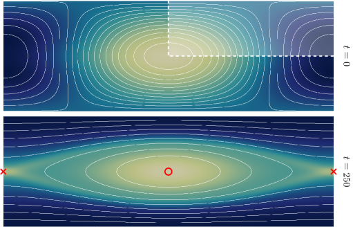
   Figure 3: Evolution of contour plots of current intensity with superimposed isolines of the magnetic vector potential $A$ (i.e., streamlines of the magnetic field), for an example solution of problem 2, with $\mu=\eta=10^{-3}$ and $\mu_{0}=1$. The top plot shows the initial conditions, with the magnetic islands induced by the perturbation; the shaded area highlights the actual domain of the simulation (notice the $y$-axis has been cropped to better zoom on the islands). As time proceeds, the islands start attracting each other until reconnection occurs in the middle plot, where we see the associated electric discharge. In the last plot the reconnection has completed, and the two islands have coalesced into one.

   Figure 4: Velocity magnitude and streamlines (left), and pressure contour plot (right) for an example solution of the flow in the island coalescence problem 2 at reconnection $t=7$, with $\mu=\eta=10^{-3}$ and $\mu_{0}=1$. Only the simulation domain (top-left corner in Fig. 3) is shown.

   As in problem 1, we start from a quiet state,

   $$\bar{{\boldsymbol{u}}}^{0}_{IC}({\boldsymbol{x}})=0.$$ (48)

   with the vector potential given by a modification to the Harris sheet equilibrium in equation eq. 44. Note that $*_{IC}$ refers to conditions for the island coalescence problem. This is at times referred to as Fadeev or Schmid-Burgk equilibrium, since they pioneered its study in [24, 25], or also as corrugated sheet pinch equilibrium [23, Chap. 4.3], and is given by

   $$A^{eq}_{IC}({\boldsymbol{x}})=\frac{1}{2\pi}\ln\left[\cosh(2\pi y)+\beta\cos(2\pi x)\right],$$ (49)

   for a given parameter $\beta$. This too must be sustained by an external electric field, in this case given by

   $$E^{eq}_{IC}({\boldsymbol{x}})=\frac{\eta}{\mu_{0}}\nabla^{2}A^{eq}_{IC}({\boldsymbol{x}})=\frac{\eta}{\mu_{0}}\frac{2\pi(1-\beta^{2})}{(\cosh(2\pi y)+\beta\cos(2\pi x))^{2}}.$$ (50)

   The flow equilibrium is maintained by a counterbalancing pressure,

   $$p^{eq}_{IC}({\boldsymbol{x}})=\frac{1}{2\mu_{0}}\frac{1-\beta^{2}}{\left(\cosh(2\pi y)+\beta\cos(2\pi x)\right)^{2}}-\bar{p}^{eq}_{IC},$$ (51)

   where again the quantity $\bar{p}^{eq}_{IC}$ is chosen to ensure the equilibrium pressure is zero-mean valued. This equilibrium is perturbed by considering as initial conditions for the vector potential

   $$\bar{A}^{0}_{IC}({\boldsymbol{x}})=A^{eq}_{IC}({\boldsymbol{x}})+\varepsilon\cos\left(\frac{\pi}{2}y\right)\cos(\pi x).$$ (52)

   Similarly to problem 1, in this case, the resulting solution is periodic in $x\in[0,2]$ and presents a number of symmetries, which we exploit to simplify our simulation and reduce the domain from $[0,2]\times[-1,1]$ to its top-left corner $\Omega=\Omega_{\square}=[0,1]^{2}$. We impose symmetry on the $x=0$, $x=1$ and $y=0$ axes, while on $y=1$, we prescribe Dirichlet BC for $A$ (again fixed to the equilibrium eq. 49), and slip conditions for ${\boldsymbol{u}}$, rendering the flow fully enclosed also in this case. The parameters considered for this problem are $\beta=0.2$ and $\varepsilon=10^{-3}$.

In our experiments, the choice of finite-element approximation for the discretisation of the functional spaces falls on the Taylor-Hood $P_{3}-P_{2}$ pair for velocity and pressure [26, Chap. 17.4], while we consider $P_{1}$ for both the vector potential and the current intensity variables. This stems from considerations on Finite Element Exterior Calculus [27, 28], and from the necessity of ensuring that the two forcing terms in the momentum equation, $\nabla p$ and $j\nabla A$, can balance each other out at equilibrium.

Regarding the parameters for the problems, we put ourselves in a somewhat favourable position, by considering only $\mu=\eta=\mu_{0}=1$. While this choice has the effect of rendering some of the dynamics described in problems 1 and 2 less evident, it allows us to neglect matters regarding stability under advection-dominated regimes, which is beyond the scope of this work, and rather focus on providing a general indication of the space-time preconditioner performance.

The actual code used for the numerical simulations is an expansion of the one developed for [16]: as such, it still relies on MFEM, PETSc, and hypre [29, 30, 31] for the linear solvers necessary to tackle the linearised system eq. 4 at each Newton iteration. As an initial guess for the discrete space-time velocity, pressure, and vector potential, we pick the projection of the equilibrium conditions, eq. 43, eq. 46, eq. 44 and eq. 48, eq. 51, eq. 49, onto their respective discrete finite element spaces; the additional variable $j$ is instead initialised as the solution to its associated discrete system in eq. 2

$${\mathcal{M}}_{j}{\boldsymbol{j}}^{k}=-{\mathcal{K}}_{jA}{\boldsymbol{A}}^{k}+{\boldsymbol{h}}^{k},\qquad\forall k=1,\dots,N_{t},$$ (53)

where ${\boldsymbol{A}}^{k}$ is the initial guess on the vector potential at instant $k$, so that the initial residual associated with this variable is effectively $0$.

4.2 Performance of preconditioner

This section is dedicated to measuring the effectiveness of the proposed space-time preconditioner for accelerating the iterative solution of the linearised incompressible resistive MHD system eq. 4. In order to evaluate the preconditioner performance, we focus on tracking the number of iterations necessary to achieve convergence, for both the outer Newton solver and the inner GMRES solver. This parameter represents a more indicative measure of the behaviour of the preconditioner than, e.g., time-to-solution, as the latter strongly depends on implementation choices. This becomes even more significant given the possible challenges represented by step 2, and particularly by the inversion of $\tilde{C}_{A}$ in eq. 31, whose effective time parallelisation we do not investigate further in this work.

For similar reasons, in this study we consider only the use of exact solvers for inverting the relevant block operators appearing in $P_{T}$. That is to say, we employ sequential time-stepping for the solution of the space-time operators $F_{{\boldsymbol{u}}}$ and $\tilde{C}_{A}$, and use LU factorisation for inverting the single blocks in their block diagonals ${\mathcal{F}}_{{\boldsymbol{u}},k}$ and $\tilde{{\mathcal{C}}}_{A,k}$ (see their definitions in eq. 19 and eq. 31), as well as the vector potential mass matrix ${\mathcal{M}}_{A}$ (appearing within $M_{A}$ in eq. 33), the current intensity mass matrix ${\mathcal{M}}_{j}$ (present in $M_{j}$ in eq. 34), and the pressure mass and stiffness operators apprearing in equation eq. 13.

We also only present results for the simplified block upper-triangular preconditioner $P_{T}$ in eq. 39, since early experiments showed negligible difference in convergence behaviour with respect to using its full version $P$ from eq. 35. This makes $P_{T}$ a much more appealing choice, given how its associated computational cost is significantly reduced, as per the discussion in Sec. 3.3.

Table 1: Iterations to convergence for Newton’s method applied for the solution of problems 1 and 2, for various refinement levels of the spatial and temporal grids (the temporal domain is fixed at $T=1$). The outer solver achieves convergence with a tolerance of $10^{-10}$. The inner GMRES solver is right-preconditioned with $P_{T}$ eq. 39, and converges with relative tolerance $10^{-2}$ or absolute tolerance of $10^{-14}$. To invert the relevant operators appearing in $P_{T}$, we use exact solvers (time-stepping and LU). Inside each column, the number of Newton iterations to convergence is reported on the left, the average number of inner GMRES iterations per outer Newton iteration appears on the right (in parentheses).

Pb	${\begin{array}[]{@{}r@{}}\scriptstyle\Delta t\smash{\eqmakebox[ind]{$\scriptstyle\rightarrow$}}\\[-3.0pt] \scriptstyle\Delta x\smash{\eqmakebox[ind]{$\scriptstyle\downarrow$}}\end{array}}$	$2^{-2}$		$2^{-3}$		$2^{-4}$		$2^{-5}$		$2^{-6}$		$2^{-7}$
1	$2^{-2}$	$5$	$(7.80)$	$5$	$(9.40)$	$5$	$(11.60)$	$5$	$(13.20)$	$5$	$(13.60)$	$5$	$(16.40)$
	$2^{-3}$	$5$	$(8.40)$	$5$	$(10.20)$	$5$	$(13.00)$	$5$	$(14.80)$	$5$	$(15.00)$	$5$	$(16.60)$
	$2^{-4}$	$5$	$(8.00)$	$5$	$(10.40)$	$5$	$(12.20)$	$5$	$(13.80)$	$5$	$(15.40)$	$5$	$(17.20)$
	$2^{-5}$	$5$	$(7.40)$	$5$	$(9.40)$	$5$	$(12.00)$	$5$	$(13.40)$	$5$	$(14.00)$	$5$	$(18.40)$
	$2^{-6}$	$5$	$(7.60)$	$5$	$(9.40)$	$5$	$(12.00)$	$5$	$(13.40)$	$5$	$(13.80)$	$5$	$(17.00)$
	$2^{-7}$	$5$	$(7.60)$	$5$	$(9.80)$	$5$	$(11.80)$	$5$	$(13.20)$	$5$	$(14.40)$	$5$	$(16.80)$
2	$2^{-2}$	$4$	$(8.75)$	$5$	$(11.00)$	$5$	$(11.80)$	$5$	$(14.20)$	$4$	$(15.75)$	$4$	$(17.00)$
	$2^{-3}$	$5$	$(9.20)$	$4$	$(11.50)$	$4$	$(13.00)$	$4$	$(14.75)$	$4$	$(16.75)$	$4$	$(18.75)$
	$2^{-4}$	$4$	$(9.75)$	$4$	$(11.25)$	$4$	$(13.50)$	$4$	$(15.50)$	$4$	$(17.25)$	$4$	$(19.25)$
	$2^{-5}$	$4$	$(8.00)$	$4$	$(11.00)$	$4$	$(13.75)$	$4$	$(15.25)$	$3$	$(15.67)$	$3$	$(20.33)$
	$2^{-6}$	$3$	$(8.00)$	$3$	$(10.00)$	$3$	$(12.33)$	$3$	$(14.00)$	$3$	$(15.67)$	$3$	$(17.33)$
	$2^{-7}$	$3$	$(7.67)$	$3$	$(10.67)$	$3$	$(12.33)$	$3$	$(14.00)$	$3$	$(16.00)$	$3$	$(17.67)$

In Tab. 1 we report convergence results for both inner and outer solvers, collected for various choices of spatial and temporal grid sizes $\Delta x$ and $\Delta t$, on a fixed temporal domain of size $T=1$. There, we see how the number of Newton iterations necessary for convergence remains largely unchanged, regardless of the mesh chosen. The number of GMRES iterations seems to be increasing very slowly with temporal refinement, where increasing the number of temporal nodes by a factor of $2^{5}$ results in slightly more than $\sim 2$ times as many iterations). To put these numbers into perspective, notice that for these experiments the spatial unknowns for the most refined discretisation of problem 1 amount to $N_{{\boldsymbol{u}}}=222722$, $N_{p}=49665$, $N_{j}=N_{A}=12545$, while those for problem 2 reach $N_{{\boldsymbol{u}}}=296450$, $N_{p}=66049$, $N_{j}=N_{A}=16641$. Considering that the temporal grids count up to $N_{t}=128$ points, this results in space-time systems of total size $(N_{\boldsymbol{u}}+N_{p}+N_{j}+N_{A})\cdot N_{t}\approx 38\cdot 10^{6}$ and $\approx 52\cdot 10^{6}$ for the two problems, respectively.

The temporal domain $T=1$ considered for the experiments in Tab. 1 is however too small to allow for the relevant nonlinear behaviours described in Sec. 4.1 to manifest themselves into the solution (notice the time labels on the side of Fig. 1 and 3). To get an idea of how the preconditioner performs when these behaviours become evident, we consider another set of experiments, where we fix the time-step and progressively increase the size of the time domain. The corresponding convergence results are reported in Tab. 2. Overall, they draw a similar picture as those in Tab. 1, but with the number of inner iterations showing no growth in this case. Thus, the preconditioner is mildly sensitive in this case to the size of $\Delta t$, but not the number of time-steps.

Table 2: Convergence results for Newton iterations applied for the solution of problems 1 and 2, for various refinement levels of the spatial grid. We fix $\Delta t=0.5$, and progressively enlarge the temporal domain to accommodate for more processors. The solvers used are as in Tab. 1. Inside each column, the number of Newton iterations to convergence is reported on the left, the average number of inner GMRES iterations per outer Newton iteration appears on the right (in brackets).

Pb	${\begin{array}[]{@{}r@{}}\scriptstyle T\smash{\eqmakebox[ind]{$\scriptstyle\rightarrow$}}\\[-3.0pt] \scriptstyle\Delta x\smash{\eqmakebox[ind]{$\scriptstyle\downarrow$}}\end{array}}$	$2^{2}$		$2^{3}$		$2^{4}$		$2^{5}$		$2^{6}$		$2^{7}$
1	$2^{-2}$	$5$	$(5.80)$	$5$	$(6.20)$	$5$	$(6.20)$	$5$	$(6.60)$	$5$	$(6.40)$	$5$	$(6.40)$
	$2^{-3}$	$5$	$(6.80)$	$5$	$(6.80)$	$5$	$(6.80)$	$5$	$(6.80)$	$5$	$(6.80)$	$5$	$(6.80)$
	$2^{-4}$	$5$	$(6.60)$	$5$	$(6.60)$	$5$	$(6.60)$	$5$	$(6.60)$	$5$	$(6.60)$	$5$	$(6.80)$
	$2^{-5}$	$4$	$(6.00)$	$5$	$(6.20)$	$4$	$(6.25)$	$4$	$(6.25)$	$5$	$(6.40)$	$5$	$(6.40)$
	$2^{-6}$	$4$	$(6.00)$	$4$	$(6.00)$	$4$	$(6.00)$	$4$	$(6.00)$	$4$	$(6.25)$	$4$	$(6.25)$
	$2^{-7}$	$4$	$(5.75)$	$4$	$(6.00)$	$4$	$(6.00)$	$4$	$(6.00)$	$4$	$(6.00)$	$4$	$(6.00)$
2	$2^{-2}$	$5$	$(6.40)$	$5$	$(6.40)$	$5$	$(6.40)$	$5$	$(6.40)$	$5$	$(6.40)$	$5$	$(6.40)$
	$2^{-3}$	$4$	$(6.75)$	$5$	$(7.00)$	$5$	$(7.00)$	$5$	$(7.00)$	$5$	$(7.00)$	$5$	$(7.00)$
	$2^{-4}$	$4$	$(6.25)$	$4$	$(6.25)$	$4$	$(6.50)$	$4$	$(6.75)$	$5$	$(6.80)$	$5$	$(6.80)$
	$2^{-5}$	$4$	$(6.50)$	$4$	$(6.50)$	$4$	$(6.75)$	$4$	$(6.50)$	$4$	$(6.50)$	$4$	$(6.50)$
	$2^{-6}$	$3$	$(6.33)$	$4$	$(6.75)$	$4$	$(6.75)$	$4$	$(6.75)$	$4$	$(6.75)$	$4$	$(6.75)$
	$2^{-7}$	$3$	$(6.33)$	$3$	$(6.33)$	$3$	$(6.33)$	$3$	$(6.33)$	$4$	$(6.75)$	$3$	$(6.33)$

4.3 Comparison with sequential time-stepping

In this section, we provide an indication of how the number of inner and outer iterations to convergence for the space-time preconditioner $P_{T}$, ($N_{it,L}^{ST}$ and $N_{it,NL}^{ST}$), compare with those of its single time-step counterpart ${\mathcal{P}}_{T,k}$, ($N_{it,L}^{0}$ and $N_{it,NL}^{0}$), for the test cases introduced in Sec. 4.1.

In order to conduct a balanced comparison between the single time-step and the whole space-time approaches, we adjust the absolute tolerance of the linear solver for the former by scaling it by a factor $\sqrt{N_{t}}$. For the whole space-time approach, we do the same for the outer solver, but leave the absolute tolerance of the inner solver untouched (this might slightly favour the time-stepping approach, but convergence of GMRES occurred due to the relative tolerance being met in almost all of cases). Lastly when time-stepping, we reuse the solution value from the previous time-step as the initial guess for the Newton solver at the following time-step.

Table 3: Ratios $N_{it,NL}^{ST}/N_{it,NL}^{0}$ and $N_{it,L}^{ST}/N_{it,L}^{0}$, where $N_{it,NL}^{ST}$ and $N_{it,L}^{ST}$ are the total number of outer and inner iterations to convergence for the space-time approach (resulting from the same experiments used to fill Tab. 1), while $N_{it,NL}^{0}$ and $N_{it,L}^{0}$ represent the average number of outer and inner iterations to convergence per time-step, using time-stepping. For the latter, the inner solver for each time-step is GMRES, right-preconditioned with the single time-step counterpart of the block upper-triangular preconditioner, eq. 40. The outer solver for time-stepping reaches convergence with absolute tolerance $10^{-10}/\sqrt{N_{t}}$, while the inner solver has the same tolerances used for Tab. 1. For some of the most extreme parameters combinations, we noticed that the solution from time-stepping “freezes” from a certain (reasonably late) instant onwards: that is, the residual after the Newton update becomes smaller than the prescribed tolerance, thus preventing any other update from being carried out (notice we do not implement mesh adaptivity). To account for this, we compute the averages $N_{it,NL}^{0}$ and $N_{it,L}^{0}$ by considering the effective time-steps only.

Pb	${\begin{array}[]{@{}r@{}}\scriptstyle\Delta t\smash{\eqmakebox[ind]{$\scriptstyle\rightarrow$}}\\[-3.0pt] \scriptstyle\Delta x\smash{\eqmakebox[ind]{$\scriptstyle\downarrow$}}\end{array}}$	$2^{-2}$		$2^{-3}$		$2^{-4}$		$2^{-5}$		$2^{-6}$		$2^{-7}$
1	$2^{-2}$	$1.05$	$(1.05)$	$1.14$	$(1.18)$	$1.31$	$(1.45)$	$1.38$	$(1.54)$	$1.63$	$(1.97)$	$1.66$	$(2.41)$
	$2^{-3}$	$1.11$	$(1.17)$	$1.18$	$(1.29)$	$1.27$	$(1.54)$	$1.45$	$(1.80)$	$1.54$	$(2.15)$	$1.65$	$(2.40)$
	$2^{-4}$	$1.11$	$(1.21)$	$1.21$	$(1.40)$	$1.40$	$(1.65)$	$1.47$	$(1.82)$	$1.50$	$(2.35)$	$1.65$	$(2.73)$
	$2^{-5}$	$1.11$	$(1.13)$	$1.25$	$(1.38)$	$1.45$	$(1.79)$	$1.55$	$(1.93)$	$1.66$	$(2.51)$	$1.86$	$(3.50)$
	$2^{-6}$	$1.11$	$(1.21)$	$1.33$	$(1.50)$	$1.48$	$(1.89)$	$1.60$	$(2.06)$	$1.72$	$(2.71)$	$1.91$	$(3.52)$
	$2^{-7}$	$1.25$	$(1.42)$	$1.29$	$(1.56)$	$1.51$	$(1.94)$	$1.68$	$(2.21)$	$1.77$	$(3.06)$	$2.01$	$(3.91)$
2	$2^{-2}$	$1.07$	$(1.12)$	$1.54$	$(1.73)$	$1.57$	$(1.78)$	$1.72$	$(2.25)$	$1.48$	$(2.13)$	$1.59$	$(2.44)$
	$2^{-3}$	$1.54$	$(1.79)$	$1.39$	$(1.76)$	$1.60$	$(2.05)$	$1.60$	$(2.41)$	$1.70$	$(3.25)$	$1.79$	$(3.70)$
	$2^{-4}$	$1.23$	$(1.53)$	$1.45$	$(1.90)$	$1.60$	$(2.23)$	$1.78$	$(2.68)$	$1.95$	$(4.36)$	$2.18$	$(5.26)$
	$2^{-5}$	$1.45$	$(1.60)$	$1.45$	$(1.96)$	$1.78$	$(2.67)$	$2.03$	$(3.19)$	$1.60$	$(3.40)$	$1.90$	$(5.36)$
	$2^{-6}$	$1.09$	$(1.33)$	$1.26$	$(1.63)$	$1.55$	$(2.20)$	$1.57$	$(2.38)$	$1.79$	$(4.21)$	$1.98$	$(5.20)$
	$2^{-7}$	$1.20$	$(1.39)$	$1.41$	$(2.00)$	$1.60$	$(2.38)$	$1.75$	$(2.83)$	$1.88$	$(5.01)$	$2.04$	$(5.99)$

Given the discussion in Sec. 3.4, it is clear that both ratios $N_{it,L}^{ST}/N_{it,L}^{0}$ and $N_{it,NL}^{ST}/N_{it,NL}^{0}$ must be kept as close as possible to $1$ for the space-time preconditioning approach to represent an appealing alternative to sequential time-stepping. The results in Tab. 3 show that this condition is satisfied reasonably well: the ratio of Newton iterations hits a maximum of $\sim 2$, while that of GMRES iterations sits between $1$ and $3$ for most cases. As $\Delta t\to 0$, this ratio tends to increase, reaching almost $6$ in certain instances. This is not surprising, as in this case the small time step sizes improve the quality of the initial guess for Newton’s method during sequential time-stepping. We note that these parallel-in-time overheads are favourable for the field [32].

Overall, the results in this section showcase the potential effectiveness of our space-time block preconditioning approach in this more complex MHD case. At least when employing exact solvers, the space-time preconditioner requires limited overhead in terms of number of iterations to convergence with respect to its single time-step equivalent. This allows significant room for parallel efficiency, so long as effective PinT methods are developed to solve the single-variable space-time systems appearing within our preconditioner, namely involving operators $F_{{\boldsymbol{u}}}$ and $\tilde{C}_{A}$. Success has already been shown for solving such single-variable space-time systems in parallel, e.g., [33, 34, 35].

5 Conclusions

In this work, we develop an all-at-once space-time preconditioner for resistive MHD. In formulating our preconditioner, we follow the space-time block preconditioning principle first outlined in [16]. There, an application to incompressible flow is considered, where a suitable block preconditioning strategy for sequential time-stepping (namely, PCD [20]) is extended to the all-at-once, space-time setting. In this work, we showcase how this same principle can be applied to more complicated PDEs. In particular, we focus on applications in resistive MHD, and extend the continuous Schur complement preconditioner introduced in [10] from the sequential time-stepping to the space-time setting. We thus produce, to our knowledge, the first space-time block preconditioning approach for this problem (or any problem aside from Navier Stokes). During our derivation, we consider a number of simplifications and approximations from a direct block LU decomposition to arrive at a practical space-time preconditioner, which only requires the parallel solution of inner time-dependent single-variable equations, rather than the original time-dependent and nonlinearly coupled sets of equations.

The numerical results are promising, with the overhead associated with space-time preconditioning versus sequential time-stepping modest in Table 3, typically in the range of $2\times$–$5\times$. We note that such overhead is small for a parallel-in-time scheme [32]. Additionally, the scaling results for inner (linear) and outer (nonlinear) iterations are flat in the case of fixed $\Delta t$ and only very slowly growing in the case of refinements in time, providing further evidence for the quality of the preconditioner proposed. Our experiments here rely on using exact block inverses for the inner scalar (but still space-time) equations, as this initial work focuses on the design of the overall space-time block preconditioning approach, which is a first for MHD. Future work will study the development of suitable iterative schemes for the individual space-time blocks, especially $F_{{\boldsymbol{u}}}$ and $\tilde{C}_{A}$, where we will leverage previous work on nonsymmetric AMG [33, 36, 37].

References

- [1] UK Atomic Energy Authority, Culham Centre for Fusion Energy, https://ccfe.ukaea.uk/.
- [2] R. J. Goldston, P. H. Rutherford, Introduction to plasma physics, Institute of Physics Publishing, Bristol, 1995.
- [3] R. Codina, N. Hernández-Silva, Stabilized finite element approximation of the stationary magneto-hydrodynamics equations, Computational Mechanics 38 (4) (2006) 344–355. doi:10.1007/s00466-006-0037-x.
- [4] J. H. Adler, T. R. Benson, E. C. Cyr, P. E. Farrell, S. P. MacLachlan, R. S. Tuminaro, Monolithic multigrid methods for magnetohydrodynamics, SIAM Journal on Scientific Computing 43 (5) (2021) S70–S91.
- [5] F. Laakmann, P. E. Farrell, L. Mitchell, An augmented lagrangian preconditioner for the magnetohydrodynamics equations at high Reynolds and coupling numbers, SIAM Journal on Scientific Computing 44 (4) (2022) B1018–B1044.
- [6] J. Shadid, R. Pawlowski, J. Banks, L. Chacón, P. Lin, R. Tuminaro, Towards a scalable fully-implicit fully-coupled resistive MHD formulation with stabilized FE methods, Journal of Computational Physics 229 (20) (2010) 7649–7671. doi:10.1016/j.jcp.2010.06.018.
- [7] B. Philip, L. Chacón, M. Pernice, Implicit adaptive mesh refinement for 2d reduced resistive magnetohydrodynamics, Journal of Computational Physics 227 (20) (2008) 8855–8874. doi:10.1016/j.jcp.2008.06.029.
- [8] L. Chacón, D. Knoll, J. Finn, An implicit, nonlinear reduced resistive MHD solver, Journal of Computational Physics 178 (1) (2002) 15–36. doi:10.1006/jcph.2002.7015.
- [9] J. Shadid, R. Pawlowski, E. Cyr, R. Tuminaro, L. Chacón, P. Weber, Scalable implicit incompressible resistive MHD with stabilized fe and fully-coupled Newton-Krylov-AMG, Computer Methods in Applied Mechanics and Engineering 304 (2016) 1–25. doi:10.1016/j.cma.2016.01.019.
- [10] E. C. Cyr, J. N. Shadid, R. S. Tuminaro, R. P. Pawlowski, L. Chacón, A new approximate block factorization preconditioner for two-dimensional incompressible (reduced) resistive MHD, SIAM Journal on Scientific Computing 35 (3) (2013) B701–B730. doi:10.1137/12088879X.
- [11] A.-M. Baudron, J.-J. Lautard, Y. Maday, O. Mula, The parareal in time algorithm applied to the kinetic neutron diffusion equation, in: J. Erhel, M. J. Gander, L. Halpern, G. Pichot, T. Sassi, O. Widlund (Eds.), Domain Decomposition Methods in Science and Engineering XXI, Springer International Publishing, Cham, 2014, pp. 437–445.
- [12] D. Samaddar, D. Newman, R. Sánchez, Parallelization in time of numerical simulations of fully-developed plasma turbulence using the parareal algorithm, Journal of Computational Physics 229 (18) (2010) 6558–6573. doi:10.1016/j.jcp.2010.05.012.
- [13] J. Reynolds-Barredo, D. Newman, R. Sánchez, D. Samaddar, L. Berry, W. Elwasif, Mechanisms for the convergence of time-parallelized, parareal turbulent plasma simulations, Journal of Computational Physics 231 (23) (2012) 7851–7867. doi:10.1016/j.jcp.2012.07.028.
- [14] D. Samaddar, D. Coster, X. Bonnin, L. Berry, W. Elwasif, D. Batchelor, Application of the parareal algorithm to simulations of elms in iter plasma, Computer Physics Communications 235 (2019) 246–257. doi:10.1016/j.cpc.2018.08.007.
- [15] J.-L. Lions, Y. Maday, G. Turinici, Résolution d’EDP par un schéma en temps pararéel, Comptes Rendus de l’Académie des Sciences - Series I - Mathematics 332 (7) (2001) 661 – 668. doi:10.1016/S0764-4442(00)01793-6.
- [16] F. Danieli, B. S. Southworth, A. J. Wathen, Space-time block preconditioning for incompressible flow, SIAM Journal on Scientific Computing 44 (1) (2022) A337–A363.
- [17] D. Silvester, H. Elman, D. Kay, A. Wathen, Efficient preconditioning of the linearized Navier-Stokes equations for incompressible flow, Journal of Computational and Applied Mathematics 128 (1) (2001) 261 – 279, numerical Analysis 2000. Vol. VII: Partial Differential Equations. doi:10.1016/S0377-0427(00)00515-X.
- [18] H. Elman, D. Silvester, A. Wathen, Finite Elements and Fast Iterative Solvers: with Applications in Incompressible Fluid Dynamics, Numerical Mathematics and Scientific Computation, Oxford University Press, UK, 2014. doi:10.1093/acprof:oso/9780199678792.001.0001.
- [19] E. C. Cyr, J. N. Shadid, R. S. Tuminaro, Stabilization and scalable block preconditioning for the Navier-Stokes equations, Journal of Computational Physics 231 (2) (2012) 345–363. doi:10.1016/j.jcp.2011.09.001.
- [20] H. Elman, V. Howle, J. Shadid, R. Shuttleworth, R. Tuminaro, A taxonomy and comparison of parallel block multi-level preconditioners for the incompressible Navier-Stokes equations, Journal of Computational Physics 227 (3) (2008) 1790–1808. doi:10.1016/j.jcp.2007.09.026.
- [21] H. Alfvén, Existence of electromagnetic-hydrodynamic waves, Nature 150 (3805) (1942) 405–406. doi:10.1038/150405d0.
- [22] B. S. Southworth, A. A. Sivas, S. Rhebergen, On fixed-point, Krylov, and block preconditioners for nonsymmetric problems, SIAM Journal on Matrix Analysis and Applications 41 (2) (2020) 871–900. doi:10.1137/19M1298317.
- [23] D. Biskamp, Magnetic Reconnection in Plasmas, Cambridge Monographs on Plasma Physics, Cambridge University Press, UK, 2000. doi:10.1017/CBO9780511599958.
- [24] V. M. Fadeev, I. F. Kvabtskhava, N. N. Komarov, Self-focusing of local plasma currents, Nuclear Fusion 5 (3) (1965) 202–209. doi:10.1088/0029-5515/5/3/003.
- [25] Schmid-Burgk, Zweidimensionale selbstkonsistente Lösungen der stationären Wlassowgleichung für Zweikomponententplasmen, Master’s thesis, Ludwig-Maximilians-Universität München (1965).
- [26] A. Quarteroni, Numerical Models for Differential Problems, MS&A, Springer International Publishing, 2017. doi:10.1007/978-3-319-49316-9.
- [27] D. N. Arnold, Finite Element Exterior Calculus, Society for Industrial and Applied Mathematics, Philadelphia, PA, 2018. doi:10.1137/1.9781611975543.
- [28] K. Hu, Private communication.
- [29] MFEM: Modular finite element methods [software], mfem.org. doi:10.11578/dc.20171025.1248.
-
[30]
S. Balay, S. Abhyankar, M. F. Adams, J. Brown, P. Brune, K. Buschelman,
L. Dalcin, A. Dener, V. Eijkhout, W. D. Gropp, D. Karpeyev, D. Kaushik, M. G.
Knepley, D. A. May, L. C. McInnes, R. T. Mills, T. Munson, K. Rupp, P. Sanan,
B. F. Smith, S. Zampini, H. Zhang, H. Zhang,
PETSc Web page,
https://www.mcs.anl.gov/petsc, software (2019).
URL https://www.mcs.anl.gov/petsc - [31] HYPRE: Scalable linear solvers and multigrid methods, www.llnl.gov/casc/hypre/, software.
- [32] B. W. Ong, J. B. Schroder, Applications of time parallelization, Computing and Visualization in Science 23 (11) (2020). doi:10.1007/s00791-020-00331-4.
- [33] A. A. Sivas, B. S. Southworth, S. Rhebergen, AIR algebraic multigrid for a space-time hybridizable discontinuous Galerkin discretization of advection (-diffusion), SIAM Journal on Scientific Computing 43 (5) (2021) A3393–A3416. doi:10.1137/20M1375103.
- [34] G. Horton, S. Vandewalle, A space-time multigrid method for parabolic partial differential equations, SIAM Journal on Scientific Computing 16 (4) (1995) 848–864. doi:10.1137/0916050.
- [35] M. J. Gander, M. Neumüller, Analysis of a new space-time parallel multigrid algorithm for parabolic problems, SIAM Journal on Scientific Computing 38 (4) (2016) A2173–A2208. doi:10.1137/15M1046605.
- [36] T. A. Manteuffel, S. Münzenmaier, J. Ruge, B. Southworth, Nonsymmetric reduction-based algebraic multigrid, SIAM Journal on Scientific Computing 41 (5) (2019) S242–S268. doi:10.1137/18M1193761.
- [37] T. A. Manteuffel, J. Ruge, B. S. Southworth, Nonsymmetric algebraic multigrid based on local approximate ideal restriction (AIR), SIAM Journal on Scientific Computing 40 (6) (2018) A4105–A4130. doi:10.1137/17M1144350.