Physics-informed machine learning of the correlation functions in bulk fluids

Abstract

The Ornstein-Zernike (OZ) equation is the fundamental equation for pair correlation function computations in the modern integral equation theory for liquids. In this work, machine learning models, notably physics-informed neural networks and physics-informed neural operator networks, are explored to solve the OZ equation. The physics-informed machine learning models demonstrate great accuracy and high efficiency in solving the forward and inverse OZ problems of various bulk fluids. The results highlight the significant potential of physics-informed machine learning for applications in thermodynamic state theory.

I Introduction

Statistical mechanics has been successful as a framework for modeling complex systems from microscale to macroscale.Kardar (2007); Tuckerman (2010) The integral equation theory (IET) approach for liquids is one of the most widely used approaches that is based on statistical mechanics.Hirata (2003); Hansen and McDonald (2013); Cao et al. (2019) It provides a closed analytical relation between the molecular interaction potentials and microscopic correlation functions of liquids and liquid mixtures. The prediction of macroscopic properties from the knowledge of the microscopic structure allows for a detailed description of a wide diversity of bulk fluids. The basic concept in the theory is the Ornstein–Zernike (OZ) equation.Ornstein and Zernike (1914a) With the aid of statistical mechanics, along with some approximation methods such as hypernetted chain (HNC), Percus-Yevick (PY), and Verlet modified (VM)Hansen and McDonald (2013); Choudhury and Ghosh (2002); Tsednee and Luchko (2019); Carvalho and Braga (2021); Bedolla, Padierna, and Castañeda-Priego (2022) closure approximations, many properties of bulk fluids can be calculated. The OZ equation has practical importance as a foundation for approximations for computing the pair correlation function of molecules or ions, or of colloidal particles in solution.Eckert et al. (2020); Tschopp and Brader (2021) Furthermore, based on the OZ equation, several approaches such as the molecular Ornstein–Zernike (MOZ) equationRichardi, Fries, and Krienke (1998) and the three-dimensional reference interaction site model (3D-RISM) theoryBeglov and Roux (1997); Yoshida (2017); Cao, Kalin, and Huang (2023) have been developed. These theories offer a rigorous framework for calculating equilibrium solvation properties without the need for costly dynamic simulations, which can be crucial for biochemical process and drug design.Sindhikara and Hirata (2013); Samways et al. (2021); Ratkova, Palmer, and Fedorov (2015) The integral equation theory of molecular liquids has been an active area of academic research.

In recent years, the development of machine learning (ML) techniques offers a suite of powerful tools in function approximation and equation solving.Goodfellow, Bengio, and Courville (2016) ML approaches have been successfully applied to problems such as solving the direct correlation function of materialsCarvalho and Braga (2020, 2022a) or learning closures within the OZ frameworkGoodall et al. (2021). Among ML techniques, physics-informed neural networksRaissi, Perdikaris, and Karniadakis (2019) (PINNs) , are a novel type of neural network that exploit the known laws of physics by including them in the loss function. PINNs are designed to address systems governed by established laws of physics. Their versatility allows them to tackle a range of challenges, ranging from elementary algebraic equations to sophisticated physical phenomena, notably fluid dynamicsCai et al. (2021a); Raissi, Yazdani, and Karniadakis (2020); Chen et al. (2021), heat transferCai et al. (2021b); Hennigh et al. (2021). However, PINNs can sometimes struggle with the complexities introduced by parameterized partial differential equations (PDEs). Such PDEs can include parameters that are related to specific material properties, which can increase significantly the required complexity of a general-purpose neural network. The deep operator networkLu et al. (2021) (DeepOnet) is designed for operator learning, where the inputs are processed separately and then combined to produce the final output. Hence, by substituting the general-purpose neural network with DeepOnet within the PINN framework, the physics-informed deep operator network (PIDeepOnet) is well-suited for handling parameterized PDEs. Currently, the application of PINN or PIDeepOnet in IET is relatively rare. Carvalho and Braga Carvalho and Braga (2022b) developed a PINN model to solve the OZ equation and obtained impressive prediction results for the direct correlation function, showcasing the potential of PINNs in solving OZ equations. However, the complexity of their neural network architecture results in slow training. Furthermore, there is potential for enhancing prediction accuracy, particularly for the long-range correlation at higher densities.

In this work, we build a new physics-informed machine learning framework. This includes a PINN approach tailored for fixed-parameter OZ equations and a PIDeepOnet approach for parameterized OZ equations. By integrating IET with cutting-edge machine learning techniques—like Fourier feature embeddingTancik et al. (2020), the modified feedforward neural networkWang, Teng, and Perdikaris (2021), and the self-adaptive weighting methodMcClenny and Braga-Neto (2020), we achieve marked improvements in accuracy and computational efficiency compared to the existing PINN approach.Carvalho and Braga (2022b). Furthermore, the PIDeepOnet offers the potential to apply IET for fluids across diverse thermodynamic states Jaiswal, Bharadwaj, and Singh (2014); Chandler (2003).

II Methodology

II.1 The OZ equation approach to the physics of simple fluids

As a rigorous framework in statistical mechanics, the OZ equation Ornstein and Zernike (1914b) plays a vital role in approximating correlations among particles in fluids. The OZ equation has practical importance as a foundation for approximations for computing the pair correlation function of molecules or particles in liquids. The pair correlation function is related via Fourier transform to the static structure factor, which can be determined experimentally using X-ray diffraction or neutron diffraction. For the simplest case, i.e., a homogeneous isotropic fluid with density $\rho$, the total correlation function $h(r)$ is given by

$$h(r)=g(r)-1,$$ (1)

where the function $g(r)$ is the two-body correlation function. It is the probability of finding a particle a distance $r$ from another particle at 0. This probability in a liquid becomes one for large enough $r$. The OZ equation establishes a relationship between the total correlation function $h(r)$ and the direct correlation function $c(r)$ as follows:

$$h(r)=c(r)+\rho\int{c(|r-r^{\prime}|)h(r^{\prime})dr^{\prime}},$$ (2)

where $\rho$ is the number density of the system. As both functions $h(r)$ and $c(r)$ are unknown, an additional equation is required, which is known as a closure relation. This closure typically involves a physically-motivated approximation, which greatly impacts the resultant solution. The commonly accepted form for the closure is

$$h(r)+1=\exp(-\beta u(r)+\gamma(r)+B(r)),$$ (3)

where $\gamma(r)=h(r)-c(r)$ is the indirect correlation function, $\beta=1/(k_{B}T)$, $k_{B}$ is Boltzmann constant and $T$ is the temperature. $B(r)$ is the bridge function defined for specific applications and it can be expressed as a power series in $\rho$ of irreducible diagrams. $u(r)$ represents the interaction potential between particles for a specific fluid. In this work, we opt to use the 12-6 Lennard-Jones (LJ) potential unless stated otherwise, which is defined as

$$u(r)=4\epsilon\left[\left(\frac{\sigma}{r}\right)^{12}-\left(\frac{\sigma}{r}\right)^{6}\right],$$ (4)

where $\epsilon$ and $\sigma$ are the energy and size parameters, respectively. In this work, we tested three classical closures, namely the HNC closure Hansen and McDonald (2013), PY closure Hansen and McDonald (2013) and VM closure Choudhury and Ghosh (2002).

The PY closure, where $B(r)=\ln(1+\gamma(r))-\gamma(r)$ uses a linear approximation effective for weakly correlated systems, especially hard-sphere systems. In contrast, the HNC closure where $B(r)=0$ employs a non-linear approximation that better describes strongly correlated systems, although with more computational complexity. The VM closure offers a balance between the PY and HNC closures, providing an alternative for hard-sphere systems. The bridge function for the VM closure is defined as follows:

$$B(r)=\left\{\begin{aligned} &\frac{-s^{2}}{2(1+\alpha s)}&\text{for}\quad&s\geq 0\\ &-\frac{1}{2}s^{2}&\text{for}\quad&s<0\end{aligned}\right.,$$ (5)

where $\alpha=1.01752-0.275\rho^{*}$, $\rho^{*}=\rho\sigma^{3}$ and $s(r)=\gamma(r)-\beta u_{2}(r)$. The function $u_{2}(r)$ is the perturbation potential Choudhury and Ghosh (2002); Duh and Henderson (1996), which is defined as

$$u_{2}(r)=-4\epsilon\left(\frac{\sigma}{r}\right)^{6}\exp\left(-\frac{1}{\rho^{*}}\left(\frac{\sigma}{r}\right)^{6\rho^{*}}\right).$$ (6)

II.2 Physics-informed machine learning of OZ equation

In order to solve the OZ equation by physics-informed machine learning techniques, a neural network is employed to approximate the solution with respect to the input (the network architecture will be introduced in subsection II.3). In general, the network mapping is defined as $\mathbf{y}(\mathbf{x};\boldsymbol{\theta})$, where $\mathbf{x}$ and $\mathbf{y}$ are the input and output of the network, respectively, and $\boldsymbol{\theta}$ represents the trainable parameters (weights and biases) of the network. Physical laws consist of governing equations, often formulated as partial differential equations (PDEs), and their respective boundary conditions. In general, the loss function, when constrained by physical laws, can be represented in a composite manner, namely

$$\mathcal{L}(\boldsymbol{\theta}) =\mathcal{L}_{PDE}(\boldsymbol{\theta})+\mathcal{L}_{BC}(\boldsymbol{\theta})$$ (7)

$$=\frac{1}{N_{r}}\sum_{i=0}^{N_{r}}{\mathcal{N}^{2}(\mathbf{y}(\mathbf{x}_{i}^{r}))}+\frac{1}{N_{b}}\sum_{i=0}^{N_{b}}{\mathcal{B}^{2}(\mathbf{y}(\mathbf{x}_{i}^{b}))},$$

where $\mathcal{N}$ and $\mathcal{B}$ represent the residuals of the operator corresponding to the governing equations and the boundary conditions, respectively. $N_{r}$ and $N_{b}$ are the sizes of residual data set $\{\mathbf{x}_{i}^{r}\}_{i=1}^{N_{r}}$ and boundary data set $\{\mathbf{x}_{i}^{b}\}_{i=1}^{N_{b}}$.

The network is trained by minimizing the loss function. To cope with the complexity engendered by the multiple components of the loss function, it is essential to further balance these terms with adaptive weights Wang, Yu, and Perdikaris (2022). During training, we adopt a recently proposed self-adaptive weighting method McClenny and Braga-Neto (2020), which is briefly introduced in the following. By assigning a weight to each individual training point, the loss function in Eq. (7) is recast as

$$\begin{aligned} \mathcal{L}(\boldsymbol{\theta},\mathbf{w})&=\frac{1}{N_{r}}\sum_{i=0}^{N_{r}}{M(w_{i}^{r})\mathcal{N}^{2}(\mathbf{y}(\mathbf{x}_{i}^{r}))}\\ &+\frac{1}{N_{b}}\sum_{i=0}^{N_{b}}{M(w_{i}^{b})\mathcal{B}^{2}(\mathbf{y}(\mathbf{x}_{i}^{b}))}\end{aligned},$$ (8)

where $\mathbf{w}$ represents the collection of the trainable weights and $M$ denotes a mask function. In this study, we adopt the mask function $M(x)=x^{2}$, a choice that aligns with the approach taken in referenceMcClenny and Braga-Neto (2020). The optimization of the loss function given by Eq. (8), involves minimization with respect to the parameters $\boldsymbol{\theta}$, while concurrently maximizing with respect to the weights $\mathbf{w}$, namely

$$\min_{\boldsymbol{\theta}}\max_{\mathbf{w}}\mathcal{L}(\boldsymbol{\theta},\mathbf{w}).$$ (9)

In the context of a gradient ascent/descent approach, the updating of parameters and weights is carried out simultaneously, namely

$$\boldsymbol{\theta}^{k+1} =\boldsymbol{\theta}^{k}-\eta_{\boldsymbol{\theta}}^{k}\nabla_{\boldsymbol{\theta}}\mathcal{L}(\boldsymbol{\theta}^{k},\mathbf{w}^{k})$$ (10)

$$\mathbf{w}^{k+1} =\mathbf{w}^{k}+\eta_{\mathbf{w}}^{k}\nabla_{\mathbf{w}}\mathcal{L}(\boldsymbol{\theta}^{k},\mathbf{w}^{k})$$

where $k$ represents the training iteration index, while $\eta_{\boldsymbol{\theta}}^{k}$ and $\eta_{\mathbf{w}}^{k}$ are the learning rates for the parameters and self-adaptive weights, respectively. The gradient of the loss function with respect to the weights is computed as follows

$$\nabla_{\mathbf{w}}\mathcal{L}(\boldsymbol{\theta},\mathbf{w}) =\left\{M^{\prime}(w_{i}^{r})\mathcal{N}^{2}(\mathbf{x}_{i}^{r})\right\}_{i=1}^{N_{r}}$$ (11)

$$\cup\left\{M^{\prime}(w_{i}^{d})\mathcal{B}^{2}(\mathbf{x}_{i}^{b})\right\}_{i=1}^{N_{b}},$$

where $M^{\prime}$ is the derivative of the mask function $M$. It is worth noting that Eq. (11) can be calculated manually instead through automatic differentiation to save computational cost. In this work, we employ the OZ equation as well as the specific closure to build the physics-informed loss function to supervise the training of the network. In this work, the OZ equation (an integral equation) is occasionally termed as a PDE. Readers are advised to recognize this terminological choice.

II.3 Network architecture

For the OZ equation with fixed parameters, we use a modified feedforward neural network (FNN) recently introduced in the referenceWang, Teng, and Perdikaris (2021), which has demonstrated to be more effective than the standard FNN in mapping between input and output.

A modified FNN maps the input $\mathbf{x}$ to the output $\mathbf{y}$. Generally, a modified FNN consists of an input layer, $L$ hidden layers and an output layer. The $l$-th layer has $n_{l}$ neurons, where $l=0,1,..L,L+1$ denotes the input layer, first hidden layer,…, $L$-th hidden layer and the output layer, respectively. Note that the number of neurons of each hidden layer is the same, i.e., $n_{1}=n_{2}=...=n_{L}$. The forward propagation, i.e., the function $\mathbf{y}=f_{\text{nn}}(\mathbf{x})$ is

$$\left\{\begin{aligned} \mathbf{U}\;&=f_{act}(\mathbf{W}^{U}\mathbf{x}+\mathbf{b}^{U})&&\\ \mathbf{V}\;&=f_{act}(\mathbf{W}^{V}\mathbf{x}+\mathbf{b}^{V})&&\\ \mathbf{y}^{1}&=f_{act}(\mathbf{W}^{1}\mathbf{x}+\mathbf{b}^{1})&&\\ \mathbf{Z}^{l}&=f_{act}(\mathbf{W}^{l}\mathbf{y}^{l-1}+\mathbf{b}^{l}),&&2\leq l\leq L\\ \mathbf{y}^{l}&=(1-\mathbf{Z}^{l})\odot\mathbf{U}+\mathbf{Z}^{l}\odot\mathbf{V},&&2\leq l\leq L\\ \mathbf{y}\;&=\mathbf{y}^{L+1}=\mathbf{W}^{L+1}\mathbf{y}^{L}+\mathbf{b}^{L+1}&&\\ \end{aligned}\right.,$$ (12)

where $\mathbf{x}\in\mathbb{R}^{n_{0}}$ is the input, $\odot$ denotes point-wise multiplication, $\mathbf{y}^{l}\in\mathbb{R}^{n_{l}}$ is the output of the $l_{\text{th}}$ layer, $\mathbf{W}^{l}\in\mathbb{R}^{n_{l}}\times\mathbb{R}^{n_{l-1}}$ , $\mathbf{W}^{U}\in\mathbb{R}^{n_{1}}\times\mathbb{R}^{n_{0}}$ and $\mathbf{W}^{V}\in\mathbb{R}^{n_{1}}\times\mathbb{R}^{n_{0}}$ are the weights, and $\mathbf{b}^{l}\in\mathbb{R}^{n_{l}}$, $\mathbf{b}^{U}\in\mathbb{R}^{n_{1}}$ and $\mathbf{b}^{V}\in\mathbb{R}^{n_{1}}$ are the biases. $f_{act}$ is a point-wise activation function, and we chose the Swish activation function $f_{act}(x)=x\cdot\text{sigmoid}(x)$ Ramachandran, Zoph, and Le (2017).

For solving parameterized PDEs, the parameter is also taken as a component of the input. We resort to DeepOnet to build the input-output mapping Lu et al. (2021). A DeepOnet is made of two sub-networks, the trunk and branch, where the truck network takes spatial coordinates as input and the branch network takes the parameter as input. The output of DeepOnet is a function of the truck and branch outputs, which reads:

$$y=\sum_{i=1}^{I}{b_{i}t_{i}}+b_{0},$$ (13)

where $\mathbf{b}=\{b_{i}\}_{i=1}^{I}$ and $\mathbf{t}=\{t_{i}\}_{i=1}^{I}$ are the branch and trunk outputs, respectively. $b_{0}$ is a trainable bias variable. As for the architecture of the trunk and branch networks, we also adopt the modified FNN. So the forward propagation for the DeepOnet, i.e., the function $y=f_{\text{DeepOnet}}(\mathbf{x})$ is:

$$\left\{\begin{aligned} \mathbf{t}&=f_{\text{nn,t}}(\mathbf{x}_{t})\\ \mathbf{b}&=f_{\text{nn,b}}(\mathbf{x}_{b})\\ y&=\sum_{i=1}^{M}{b_{i}t_{i}+b_{0}}\end{aligned}\right..$$ (14)

where $f_{\text{nn,t}}$ and $f_{\text{nn,b}}$ are the forward propagation functions of the trunk and branch nets, respectively. Also, $\mathbf{x}_{t}$ and $\mathbf{x}_{b}$ are the trunk and branch inputs, respectively.

II.4 Data preprocessing

The effectiveness of neural network training is often influenced by the scale of the input/output data, as highlighted by the reference Loffe and Normalization (2014). Consequently, implementing normalization prior to training can significantly improve performance. In a given problem scenario, the lower and upper boundaries of the input vector $\mathbf{x}$ are often predefined. These can be employed to scale the input $\mathbf{x}$, making it lie within the interval $[-1,1]$ for each dimension:

$$\widetilde{\mathbf{x}} =s_{I}\left(\mathbf{x}\right)=\frac{\mathbf{x}-(\mathbf{x}_{\max}+\mathbf{x}_{\min})/2}{(\mathbf{x}_{\max}-\mathbf{x}_{\min})/2}$$ (15)

In our case, the indirect correlation function $\gamma(r)$ is known to oscillate around 0 with waves whose spectrum covers a wide range. However, PINN training can suffer from a spectral bias problem Basri et al. (2020); Rahaman et al. (2019); Wang, Wang, and Perdikaris (2021), namely, the network tends to focus on learning to low-frequency modes. To address this issue in the context of the OZ equation, we apply a straightforward transformation of the normalized coordinate $\widetilde{r}$ into multiple Fourier features, as introduced in the referenceTancik et al. (2020). The transformation is constructed by a random Fourier mapping $s_{F}:\widetilde{r}\to\mathbb{R}^{2m}$:

$$s_{F}(\widetilde{r})=\left(\sin(\pi\mathbf{B}\widetilde{r}),\cos(\pi\mathbf{B}\widetilde{r})\right),$$ (16)

where $\mathbf{B}\in\mathbb{R}^{m}$ is a random vector and $m$ is the number of Fourier features. The elements of $\mathbf{B}$ are sampled from a Gaussian distribution $b\sim N(0,\sigma_{F}^{2})$, where $\sigma_{F}^{2}$ is the feature variance. Embedding Fourier features can enhance the network’s ability to learn high-frequency modes. Using Fourier feature embedding with increased variance generally aids in capturing higher-frequency modes, though it may necessitate more residual points. Consequently, it’s essential to select the Fourier feature variance carefully based on the specific problem at hand. For more details about Fourier feature embedding, we refer to the reference Tancik et al. (2020).

For the output, a predefined range is not always available. Since there is usually not any prior knowledge about the output, the normalization is just the identical mapping, namely

$$\widetilde{\mathbf{y}}=s_{O}\left(\mathbf{y}\right)=\mathbf{y}.$$ (17)

II.5 Training details

We initiate the network using the Xavier initialization method Glorot and Bengio (2010), with weights initialized accordingly and biases set to zero. Initially, the self-adaptive weights are assigned a value of 1. The network training undergoes a two-stage process: In the first stage, we employ the Adam optimizer Kingma and Ba (2014) for 36,000 iterations. The learning rates are fixed as $\eta_{\boldsymbol{\theta}}=0.0001$ and $\eta_{\mathbf{w}}=0.1$. In the subsequent stage, the next 4,000 iterations use the L-BFGS optimizer Liu and Nocedal (1989), during which the self-adaptive weights remain unchanged.

Our training approach is implemented in PyTorch Paszke et al. (2019) and is executed on a GPU cluster. For computations, we use a 32-bit single-precision data type and a single NVIDIA^® Tesla P100 GPU.

We observed that during the L-BFGS updating phase, the training results can suddenly explode, increasing to very large magnitudes. This behavior might be attributed to the complex nonlinearity nature of the OZ equation. To counteract this, we have selected the best-trained network from prior to this explosion as our final model.

III Result and discussion

III.1 Solution of OZ equation for simple fluid

III.1.1 Forward problem

We first test the capability of the PINN approach for the OZ equation with the HNC closure. The reason we choose the HNC closure is that a previous PINN modelCarvalho and Braga (2022b) struggled with predicting long-range correlations due to its inherent nonlinearity. The parameters in the OZ equation are set as $k_{B}=\sigma=\epsilon=1$ and $T=2$. The unknown of the OZ equation, namely the indirect correlation $\gamma(r)$ is characterized by a sharp gradient for $r\to 0$, which presents a significant challenge for the training of networks. In line with the strategy presented by Carvalho and Braga (2022b), our approach takes $r$ as input, and predicts $\Gamma(r)=r\gamma(r)$ as opposed to $\gamma(r)$. This strategy assists in moderating the sharpness of the gradient, thereby facilitating improved training of the network. Similarly, we define $C(r)=rc(r)$ for the direct correlation, whose Fourier transformation Lado (1971) is calculated as

$$\widehat{C}(q_{j})=4\pi\Delta r\sum_{i=1}^{N-1}{C(r_{i})}\sin(r_{i}q_{j}),$$ (18)

where $r_{i}=i\Delta r$ for $i=0,1,...,N$, $q_{j}=j\Delta q$ for $j=0,1,...,N$, $\Delta r=\frac{R_{\max}}{N}$ and $\Delta q=\frac{\pi}{R_{\max}}$. Here, $R_{\max}=20$ is the maximum $r$ coordinate to be studied and $N=800$ is chosen. In the reciprocal space for the OZ equation, we obtain the Fourier transformation of $\Gamma(r)$ according to $\widehat{C}(q)$, namely

$$\widehat{\Gamma}(q_{j})=\frac{\rho\widehat{C}^{2}(q_{j})}{q_{j}-\rho\widehat{C}(q_{j})}.$$ (19)

Then an inverse Fourier transformation is performed to recover $\Gamma(r)$, namely

$$\Gamma^{*}(r_{i})=\frac{\Delta q}{2\pi^{2}}\sum_{j=1}^{N-1}{\widehat{\Gamma}(q_{j})\sin(r_{i}q_{j}}).$$ (20)

$\Gamma(r)$ is the prediction of network and $\Gamma^{*}(r)$ is the prediction encoded by the physical laws of OZ equation. When they are equal, the OZ equation is solved. Thus, the PDE component of the loss function is built as the mean squared error between them, namely

$$\mathcal{L}_{PDE}=\frac{1}{N-1}\sum_{i=1}^{N-1}\left[{\Gamma^{*}(r_{i})-\Gamma(r_{i})}\right]^{2}$$ (21)

The boundary condition is defined as

$$\Gamma(0)=\Gamma(R_{\max})=0.$$ (22)

Thus the loss function is defined as

$$loss =\mathcal{L}_{PDE}+\mathcal{L}_{BC}$$ (23)

$$=\frac{1}{N-1}\sum_{i=1}^{N-1}\left[{\Gamma^{*}(r_{i})-\Gamma(r_{i})}\right]^{2}+\frac{1}{2}\left[\Gamma^{2}(0)+\Gamma^{2}(R_{\max})\right].$$ (24)

For the sake of clarity, the forward propagation for deriving the PDE loss is shown in Fig. 1. The steps for calculating the PDE loss are listed as follows:

1. Predict $\Gamma(r)$ at $N-1$ equally-spaced points $r=r_{i}$ for $i=1,...,N-1$.

2. Compute $C(r)$ according to the HNC closure.

3. Perform the Fourier transformation of $C(r)$ according to Eq. (18).

4. Calculate the Fourier transformation of $\Gamma(r)$ with Eq. (19).

5. Perform the inverse Fourier transformation in Eq. (20) to recover $\Gamma^{*}(r).$

6. Calculate the PDE loss with Eq. (21).

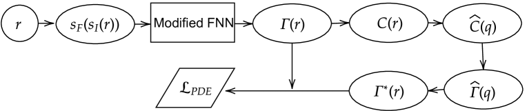
Figure 1: Forward propagation of PDE loss in the PINN approach for solving the OZ equation. $s_{I}(\cdot)$ denote the normalization function of input and $s_{F}(\cdot)$ denotes the Fourier feature transformation function.

The network is structured as $(1,30,30,30,30,30,30,1)$, with each entry denoting the neuron count for that layer. The feature variance $\sigma_{F}^{2}=1$ and the feature number $m=50$ are set for the Fourier feature embedding. As pointed out in reference Carvalho and Braga (2022b), proper initialization of a network greatly contributes to efficient and effective network training. For this purpose, we first train the network with an initialization function $y=cre^{-br}$ with $c=10$ and $b=3$. The function applies for all densities in this section and is presented in Fig. 2. Then we train the network with the PINN approach starting from the pre-trained network. Fig. 2 showcases a comparison between PINN predictions and numerical results. The latter, deemed as the ground truth, is obtained via the iterative Fourier method at a high resolution of $N=2000$. The PINN approach is able to predict the solutions accurately with a relative $L_{2}$ error $2.04\times 10^{-3},4.11\times 10^{-4},2.40\times 10^{-4}$ for density $\rho=0.1,0.5,0.9$, respectively. The performance of our model is similar to a previous PINN modelCarvalho and Braga (2022b) when the density of the simulation system is not high, e.g., less than 0.5. With the increase of density, the solution is shown to oscillate with higher frequency and larger amplitude due to the long-range correlation. Even for the large density case $\rho=0.9$, the prediction of our PINN model can still accurately capture the oscillation of small amplitude (about 0.01), as shown in the close-up view in Fig. 2. The superiority of the present PINN approach is evident, compared with results in the reference Carvalho and Braga (2022b) which fails to capture the long-range correlation ($5\leq r\leq 8$). This indicates that our model has a wider scope of application for various fluids. In addition, the training time is less than 10 minutes with a single Nvidia P100 graphics card, while the model in the previous paper would take several hours to train Carvalho and Braga (2022b). This could be attributed to the complex neural network architecture of their PINN model.

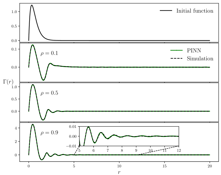
Figure 2: Initial function (1 row) and PINN predictions of $\Gamma(r)$ vs. simulation results for the OZ equation.

III.1.2 Inverse problem

The two-body static correlation function $g(r)$ is the quantity of interest in radiation scattering experiments. In this section, we use PINN to infer $g(r)$ from experimental neutron scattering data $s(q)$ (structure factor). Their relation is reflected in the following equation:

$$s(q)=1+4\pi\rho\int{\left[g(r)-1\right]r^{2}\left[\frac{sin(qr)}{qr}\right]}.$$ (25)

We use experimental data for liquid argon at 85 K.Yarnell et al. (1973) The reduced number density is $\rho=1000/36.0385^{3}$. The maximum $r$ coordinate is chosen as $R_{\max}=36$.

The network takes $r$ as input and outputs $g(r)$. The loss function is built as the mean squared error between the prediction of $s(q)$ using the network for $g(r)$ in Eq. (25) and its experimental observation $s_{exp}(q)$, namely

$$\mathcal{L}=\frac{1}{N_{q}}\sum_{i=1}^{N_{q}}\left[s(q_{i})-s_{exp}(q_{i})\right].$$ (26)

where the experimental data of $s_{exp}(q)$ contains $N_{q}=400$ points within the range $q\in(0,11.8)$. To evaluate $s(q)$ using the network for $g(r)$, the integral in Eq. (25) is approximated by the compound trapezoidal formula with $N_{r}+1$ equally-spaced points over the range $[0,R_{\max}]$. $N_{r}$ is set as 800.

For the sake of clarity, the forward propagation for the PINN approach is shown in Fig. 3. The steps for calculating the loss are listed as follows:

1. Predict $g(r)$ at $N_{r}+1$ equally-spaced points

2. Compute $s(q_{i})$ for $i=1,...,N_{q}$ according to Eq. (25).

3. Calculate the loss with Eq. (26).

Figure 3: Forward propagation in the PINN approach for solving the inverse problem. $s_{I}(\cdot)$ denote the normalization function of input and $s_{F}(\cdot)$ denotes the Fourier feature transformation function.

The network is structured as $(1,30,30,30,30,30,30,1)$, with each entry denoting the neuron count for that layer. The feature variance $\sigma_{F}^{2}=1$ and the feature number $m=50$ are set for the Fourier feature embedding. Similarly, the network is pre-trained with a initialization function, which is defined as the low density limit of the radial distribution, namely $g(r)=e^{-\frac{u(r)}{k_{B}T}}$ with $\epsilon=\sigma=1$, $k_{B}=1$ and $T=2$. The PINN predictions are shown in Fig. 4. The PINN prediction of $s(q)$ coincides well with the experimental data with a relative $L_{2}$ error $5.14\times 10^{-4}$, implying a tiny training error. In the region where $r$ is small, the PINN prediction of $g(r)$ exhibits spurious fluctuations. This behavior can be neglected because the exact $g(r)$ in this region should be 0, which is also noted in the references Carvalho and Braga (2022b); Carvalho et al. (2020). For a larger $r$, the PINN prediction of $g(r)$ agrees well with the experimental data, and the relative $L_{2}$ error is $4.48\times 10^{-3}$, when calculated over the region $3.5<r<R_{\max}$.

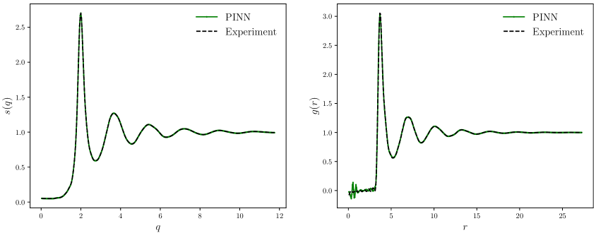
Figure 4: PINN predictions of $s(q)$ and $g(r)$ vs. experimental observations for the inverse inference of radial distribution $g(r)$.

III.2 Comparison between various closures

In this section, the PINN approach as described in Section III.1.1 is applied to solving the OZ equation with various closures respectively. The PY, HNC, and VM closures are selected. The parameters for the OZ equation are employed as $k_{B}=\sigma=\epsilon=1$ and $T=2$. The same network structure and Fourier feature embedding are employed for all the closures as well as for all the densities. As shown in Fig. 5, the PINN predictions agree well with the simulation results (using a high resolution $N=2000$), highlighting the high accuracy of our PINN approach.

When $\rho=0.1$, there is almost no difference among the three closures. This is consistent with previous workBedolla, Padierna, and Castañeda-Priego (2022). When the density is small, the physical system behaves like a gas, so the long-range correlation effect is very weak. With the increase of $\rho$, the long-range correlation effect becomes stronger, as represented by the slow decay of quasi-periodic oscillation along the $r$ direction shown in Fig.5. The prediction with VM closure shows the largest oscillation amplitude, the prediction with HNC closure has the smallest oscillation amplitude i.e., stronger long-range correlation. Our PINN model can capture the significant discrepancy of predictions of correlation function among closures even at higher density.

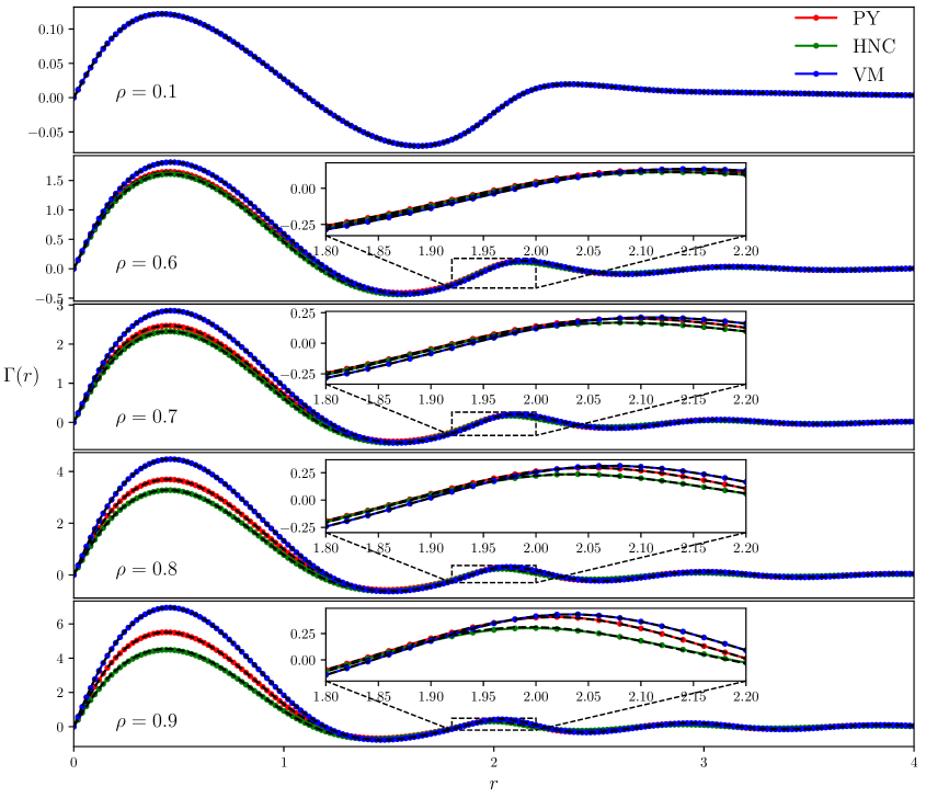
Figure 5: PINN predictions vs. simulation results of $\Gamma(r)$ for the OZ equation with the PY, HNC and VM closures. The results from the numerical simulations are depicted with black dashed lines. Remarkably, the curves from PINN predictions align so closely with the simulation results that they nearly overlap, highlighting the accuracy of the PINN approach.

III.3 Application to various types of fluids

In the above section we presented the application of PINN to the OZ equation for the LJ fluid. In this section, the PINN approach as described in Section III.1.1 is applied to solving the OZ equation using PY closure for various fluids. To compare with the numerical results in referenceBedolla, Padierna, and Castañeda-Priego (2022), the reduced temperature is set to $T=1.5$. The definition of fluid is represented by the potential function $u(r)$. In addition to the LJ fluid, we also consider another two widely studied fluids, namely, the hard-sphere (HS) fluid and square-well (SW) fluid,Carley (1983); Santos, Yuste, and López de Haro (2020) whose potential functions are defined as:

$$u_{HS}=\left\{\begin{aligned} \infty,\qquad&r<\sigma\\ 0,\qquad&r\geq\sigma\end{aligned}\right.,$$ (27)

$$u_{SW}=\left\{\begin{aligned} \infty,\qquad&r<\sigma\\ -\epsilon,\qquad&\sigma\leq r\leq\lambda\sigma\\ 0,\qquad&r>\lambda\sigma\end{aligned}\right.,$$ (28)

where $\lambda=1.5$ is the interaction range and $\epsilon$ is the well depth for the square-well fluid. The two fluids have discontinuities in their potential functions. To better resolve the discontinuities, a fine resolution of residual points is employed with $N=4000$. The PINN predictions as well as the numerical simulation results are depicted in Fig. 6. Note that our numerical simulation results are derived with high resolution $N=10000$, are consistent with previous results.Trokhymchuk et al. (2005); Henderson, Madden, and Fitts (1976) Our PINN predictions coincide well with the simulation results, highlighting the high accuracy of our PINN approach, particularly the excellent capability to capture the discontinuity for the hard-sphere and square-well fluids. Given the significant role of thermodynamic quantities in the integral theory, we aim to further validate the accuracy of the PINN approach quantitatively. We compute the compressibility factor using the virial equation of stateTsednee and Luchko (2019), especially as it has a strong connection to the discontinuous potential functions inherent to hard-sphere and square-well fluids. Its definition is given as follows:

$$P_{HS} =1+\frac{2\pi}{3}\rho\sigma^{3}g(\sigma^{+}),$$ (29)

$$P_{SW} =1+\frac{2\pi}{3}\rho\sigma^{3}(g(\sigma^{+})+\lambda^{3}(g(\lambda\sigma^{+})-g(\lambda\sigma^{-}))),$$ (30)

where $g(\sigma^{+})$ and $g(\sigma^{-})$ denote the right/left limit, respectively, of the function $g(r)$ at $r=\sigma$. Similarly, this also applies for $g(\lambda\sigma^{+})$ and $g(\lambda\sigma^{-})$. The compressibility factor $Z$ is defined as

$$Z=\beta{P}/\rho$$ (31)

Table 1 lists the predictions of the compressibility factor from this work and those from the reference Bedolla, Padierna, and Castañeda-Priego (2022), showing excellent agreement. We identified that the contribution to the total error from the discontinuity points is greater than from the middle points. And the thermodynamic property like $Z$ is mostly relevant to the values of $g(r)$ that are close to the discontinuity points. From Fig. 6, we see that the short-range correlation increases with density for all the fluids, which also enhances the local density fluctuation. Obviously, the local fluctuation in the short range is not so strong for the potential function with a smoother attractive part such as LJ fluid. The prediction error of $Z$ of the hard-sphere and square-well fluids narrows with small $\rho$ such as 0.1. And the relative error of the prediction is very small ($10^{-5}$-$10^{-4}$). When the density is 0.7, the relative error of the SW fluid is still small, but increases to $10^{-2}.$ We conclude that for a high density fluid system with strong local fluctuation, more residual points are needed to reduce the error.

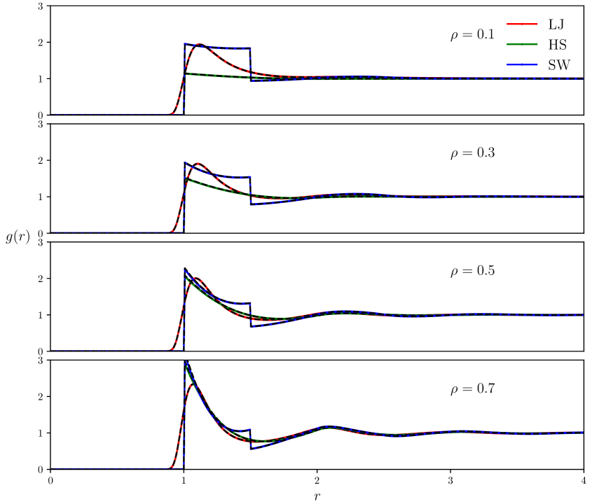
Figure 6: PINN predictions vs. simulation results of $\Gamma(r)$ for the OZ equation for the 12-6 Lennard-Jones (LJ), hard-sphere (HS), square-well (SW) fluids. The results from the numerical simulations are depicted with black dashed lines. Remarkably, the curves from PINN predictions align so closely with the simulation results that they nearly overlap, highlighting the accuracy of the PINN approach.

Table 1: Predictions of compressibility factor $Z$, where the reference value $Z_{ref}$ is derived from numerical simulations in the reference Bedolla, Padierna, and Castañeda-Priego (2022).

Density	Hard sphere fluid			Square well fluid
	$Z_{ref}$	$Z$	$|Z-Z_{ref}|/Z$	$Z_{ref}$	$Z$	$|Z-Z_{ref}|/Z$
0.1	1.23933	1.23943	7.71E-05	0.77952	0.77967	1.93E-04
0.3	1.95377	1.95520	7.34E-04	0.63587	0.63774	2.93E-03
0.5	3.17322	3.17941	1.95E-03	1.11718	1.12576	7.68E-03
0.7	5.32284	5.34269	3.73E-03	3.09157	3.12538	1.09E-02

III.4 Physics-informed DeepOnet for the solution of the parameterized OZ equation

In subsections III.1 and III.3, we used the PINN approach to solve the OZ equation with different closures, attaining substantial predictive accuracy. However, the PINN approach necessitates training the network for fixed values of the parameters. To cope with this restriction, we turn to the physics-informed DeepOnet (PIDeepOnet) approach to directly tackle the parameterized OZ equation. In this context, we treat the density $\rho\in[0.1,0.9]$ as the parameter, using the VM closure. If necessary, other thermodynamic quantities, such as temperature, can also be employed as parameters. For this case, the other parameters for the OZ equation are fixed as $k_{B}=\sigma=\epsilon=1$ and $T=2$.

The PDE loss function is constructed through repeated evaluations of Eq. (21) for different values of $\rho,$ namely

$$\mathcal{L}_{PDE}=\frac{1}{(N_{\rho}+1)(N-1)}\sum_{j=0}^{N_{\rho}}\sum_{i=1}^{N-1}\left[{\Gamma^{*}(r_{i};\rho_{j})-\Gamma(r_{i};\rho_{j})}\right]^{2}$$ (32)

where $\rho_{j}$ for $j=0,...,N_{\rho}$ are the equally-spaced points in the $\rho$ range. $N=800$ and $N_{\rho}=200$ is chosen. The boundary condition is defined as

$$\Gamma(0;\rho_{j})=\Gamma(R_{\max};\rho_{j})=0\qquad j=0,...,N_{\rho}$$ (33)

The loss function, a composite of the PDE loss and BC loss, is defined as

$$loss =\mathcal{L}_{PDE}+\mathcal{L}_{BC}$$ (34)

$$=\mathcal{L}_{PDE}+\frac{1}{2(N_{\rho}+1)}\sum_{j=0}^{N_{\rho}}\left[\Gamma(0;\rho_{j})^{2}+\Gamma(R_{\max};\rho_{j})^{2}\right]$$ (35)

For the sake of clarity, the forward propagation of the PIDeepOnet approach for deriving the PDE loss is shown in Fig. 7. The steps for calculating the PDE loss are listed as follows:

1. Predict $\Gamma(r_{i};\rho_{j})$ for $i=0,...,N$ and $j=0,...,N_{\rho}$

2. Compute $C(r;\rho)$ for each point according to the HNC closure.

3. Perform Fourier transformation for each $\rho$ according to Eq. (18).

4. Calculate the Fourier transformation of $\Gamma(r;\rho)$ for each $\rho$ with Eq. (19).

5. Perform inverse Fourier transformation for each $\rho$ with Eq. (20) to obtain $\Gamma^{*}(r;\rho)$ .

6. Calculate the PDE loss with Eq. (32).

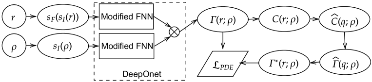
Figure 7: Forward propagation of PDE loss in the Physics-informed DeepOnet approach for solving the parameterized OZ equation. $s_{I}(\cdot)$ denote the normalization function of input and $s_{F}(\cdot)$ denotes the Fourier feature transformation function. $\otimes$ represents an inner product.

Both the trunk and branch neural networks use the same structure $(1,30,30,30,30,30,30,1)$, each entry denotes the neuron count for that layer. Note that the trunk net takes $r$ as input and the branch net takes $\rho$ as input. Fourier feature embedding is only applied to the trunk net with a variance $\sigma_{F}^{2}=1$ and the feature number $m=50$. Similarly, the network is pre-trained with an initialization function $y=c\rho re^{-br}$ with $c=30$ and $b=3$. The PIDeepOnet prediction of $\Gamma(r)$ and its absolute error is shown in Fig. 8. It is evident from the contour plot of $\Gamma(r;\rho)$ that the maximum oscillation amplitude as well as the oscillation frequency increase with $\rho$. Also, the oscillation decays slower to zero with the increase of $r$, indicating the PIDeepOnet model learned accurately the relationship between the system density and the long-range correlation. The maximum absolute error of the PIDeepOnet prediction exists near the corner ($\rho=0.9,r=0$), where the absolute value of $\Gamma(r;\rho)$ is also very large. As a result, the PIDeepOnet prediction is accurate with a relative $L_{2}$ error $6.18\times 10^{-4}$ over the domain $(r,\rho)\in[0,R_{\max}]\times[0.1,0.9]$. The extremely low relative error indicates the PIDeepOnet model is an trustworthy model for the solution of the parameterized OZ equation.

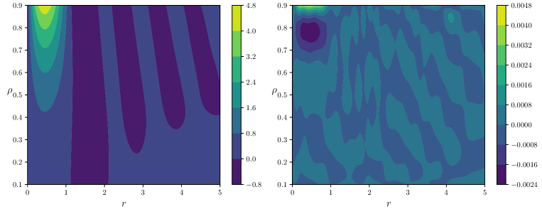
Figure 8: Predictions of $\Gamma(r)$ (left) and its absolute error (right) for parameterized OZ equations with the physics-informed DeepOnet approach.

IV Conclusion and outlook

The OZ integral equation theory is a powerful approach for computing correlations in simple fluids. In this work, we introduce a PINN approach to solve the OZ equation and a PIDeepOnet approach for tackling the parameterized OZ equation. Both the PINN and PIDeepOnet approachs are designed with state-of-the-art techniques, such as Fourier feature embedding, a modified feedforward neural network, and a self-adaptive weighting training methodology, resulting in superior accuracy and efficiency. The accuracy and robustness of the PINN approach is validated by its application to both forward and inverse OZ challenges, encompassing various closures (HNC, PY and VM closures) and fluids (12-6 Lennard-Jones, hard-sphere and square-well fluids). The PIDeepOnet approach facilitates the extension to the parameterized OZ equation by handling separately the coordinate and parameter within the DeepOnet architecture. Its capability in accurately predicting correlation functions over various thermodynamic states, offers considerable promise for advancing thermodynamic models in liquid theory.

Our PINN approach was applied to a forward OZ problem with the HNC closure. Compared to a previous PINN approachCarvalho and Braga (2022b), our PINN approach showcases enhanced accuracy, particularly for long-range correlation at high density, coupled with a significant improvement in computational efficiency. Moreover, the PINN approach was successfully applied to an inverse OZ problem, learning a correlation function according to the experimental neutron scattering data. Furthermore, the robustness of the PINN approach was further validated through applications to forward OZ problems with various closures as well as various fluid potentials. Impressively, the PINN approach is capable to of resolving discontinuous correlation functions, however it requires a higher number of residual points. Finally, the PIDeepOnet approach is employed to solve a parameterized OZ problem, taking the density as a parameter. Significantly, the relative error is at the order of $10^{-4},$ suggesting that the PIDeepOnet methodology may serve as an effective surrogate for equation-of-state models in thermodynamics, particularly in high-dimensional contexts.

Using as an example a homogeneous fluid, we have demonstrated that the PIDeepOnet model is powerful. The current approach can be extended to heterogeneous fluid and multiphase fluids. Another potential area is using the current approach with the OZ equation to infer the interaction potential function as an inverse problem, thus extracting the effective pair potential in mesoscale simulation from atomic simulation or experiment data. It is also possible to generalise and extend upon the approach adopted here by learning the closure model for a wide variety of systems where the OZ framework has been applied such as the molecular OZ and RISM approaches, and for more thermodynamic properties calculation e.g., for the solvation energy of biomolecules.

References

References

- Kardar (2007) M. Kardar, Statistical Physics of Particles (Cambridge University Press, 2007).
- Tuckerman (2010) M. Tuckerman, Statistical Mechanics: Theory and Molecular Simulation, Oxford Graduate Texts (OUP Oxford, 2010).
- Hirata (2003) F. Hirata, Molecular theory of solvation, Vol. 24 (Springer Science & Business Media, 2003).
- Hansen and McDonald (2013) J.-P. Hansen and I. R. McDonald, Theory of simple liquids: with applications to soft matter (Academic press, 2013).
- Cao et al. (2019) S. Cao, K. A. Konovalov, I. C. Unarta, and X. Huang, “Recent developments in integral equation theory for solvation to treat density inhomogeneity at solute–solvent interface,” Advanced Theory and Simulations 2, 1900049 (2019), https://onlinelibrary.wiley.com/doi/pdf/10.1002/adts.201900049 .
- Ornstein and Zernike (1914a) L. S. Ornstein and F. Zernike, “Accidental deviations of density and opalescence at the critical point of a single substance,” Proceeding of Akademic Science (Amsterdam) 17, 793–806 (1914a).
- Choudhury and Ghosh (2002) N. Choudhury and S. K. Ghosh, “Integral equation theory of Lennard-Jones fluids: A modified Verlet bridge function approach,” The Journal of Chemical Physics 116, 8517–8522 (2002), https://pubs.aip.org/aip/jcp/article-pdf/116/19/8517/10839160/8517_1_online.pdf .
- Tsednee and Luchko (2019) T. Tsednee and T. Luchko, “Closure for the ornstein-zernike equation with pressure and free energy consistency,” Phys. Rev. E 99, 032130 (2019).
- Carvalho and Braga (2021) F. Carvalho and J. Braga, “Thermodynamic consistency by a modified perkus–yevick theory using the mittag-leffler function,” Physica A: Statistical Mechanics and its Applications 576, 126065 (2021).
- Bedolla, Padierna, and Castañeda-Priego (2022) E. Bedolla, L. C. Padierna, and R. Castañeda-Priego, “Evolutionary optimization of the Verlet closure relation for the hard-sphere and square-well fluids,” Physics of Fluids 34, 077112 (2022), https://pubs.aip.org/aip/pof/article-pdf/doi/10.1063/5.0099093/16646338/077112_1_online.pdf .
- Eckert et al. (2020) T. Eckert, N. C. X. Stuhlmüller, F. Sammüller, and M. Schmidt, “Fluctuation profiles in inhomogeneous fluids,” Phys. Rev. Lett. 125, 268004 (2020).
- Tschopp and Brader (2021) S. M. Tschopp and J. M. Brader, “Fundamental measure theory of inhomogeneous two-body correlation functions,” Phys. Rev. E 103, 042103 (2021).
- Richardi, Fries, and Krienke (1998) J. Richardi, P. H. Fries, and H. Krienke, “The solvation of ions in acetonitrile and acetone: A molecular Ornstein–Zernike study,” The Journal of Chemical Physics 108, 4079–4089 (1998), https://pubs.aip.org/aip/jcp/article-pdf/108/10/4079/10789272/4079_1_online.pdf .
- Beglov and Roux (1997) D. Beglov and B. Roux, “An integral equation to describe the solvation of polar molecules in liquid water,” The Journal of Physical Chemistry B 101, 7821–7826 (1997), doi: 10.1021/jp971083h.
- Yoshida (2017) N. Yoshida, “Role of solvation in drug design as revealed by the statistical mechanics integral equation theory of liquids,” Journal of Chemical Information and Modeling 57, 2646–2656 (2017), doi: 10.1021/acs.jcim.7b00389.
- Cao, Kalin, and Huang (2023) S. Cao, M. L. Kalin, and X. Huang, “Episol: A software package with expanded functions to perform 3d-rism calculations for the solvation of chemical and biological molecules,” Journal of Computational Chemistry 44, 1536–1549 (2023), https://onlinelibrary.wiley.com/doi/pdf/10.1002/jcc.27088 .
- Sindhikara and Hirata (2013) D. J. Sindhikara and F. Hirata, “Analysis of biomolecular solvation sites by 3d-rism theory,” The Journal of Physical Chemistry B 117, 6718–6723 (2013), doi: 10.1021/jp4046116.
- Samways et al. (2021) M. L. Samways, R. D. Taylor, H. E. Bruce Macdonald, and J. W. Essex, “Water molecules at protein–drug interfaces: computational prediction and analysis methods,” Chem. Soc. Rev. 50, 9104–9120 (2021).
- Ratkova, Palmer, and Fedorov (2015) E. L. Ratkova, D. S. Palmer, and M. V. Fedorov, “Solvation thermodynamics of organic molecules by the molecular integral equation theory: Approaching chemical accuracy,” Chemical Reviews 115, 6312–6356 (2015), doi: 10.1021/cr5000283.
- Goodfellow, Bengio, and Courville (2016) I. Goodfellow, Y. Bengio, and A. Courville, Deep learning (MIT press, 2016).
- Carvalho and Braga (2020) F. Carvalho and J. Braga, “Radial distribution function for liquid gallium from experimental structure factor: a hopfield neural network approach,” Journal of Molecular Modeling 26, 193 (2020).
- Carvalho and Braga (2022a) F. S. Carvalho and J. P. Braga, “Partial radial distribution functions for a two-component glassy solid, gese3, from scattering experimental data using an artificial intelligence framework,” Journal of Molecular Modeling 28, 99 (2022a).
- Goodall et al. (2021) R. E. Goodall et al., “Data-driven approximations to the bridge function yield improved closures for the ornstein–zernike equation,” Soft Matter 17, 5393–5400 (2021).
- Raissi, Perdikaris, and Karniadakis (2019) M. Raissi, P. Perdikaris, and G. E. Karniadakis, “Physics-informed neural networks: A deep learning framework for solving forward and inverse problems involving nonlinear partial differential equations,” Journal of Computational physics 378, 686–707 (2019).
- Cai et al. (2021a) S. Cai, Z. Mao, Z. Wang, M. Yin, and G. E. Karniadakis, “Physics-informed neural networks (pinns) for fluid mechanics: A review,” Acta Mechanica Sinica 37, 1727–1738 (2021a).
- Raissi, Yazdani, and Karniadakis (2020) M. Raissi, A. Yazdani, and G. E. Karniadakis, “Hidden fluid mechanics: Learning velocity and pressure fields from flow visualizations,” Science 367, 1026–1030 (2020).
- Chen et al. (2021) W. Chen, Q. Wang, J. S. Hesthaven, and C. Zhang, “Physics-informed machine learning for reduced-order modeling of nonlinear problems,” Journal of computational physics 446, 110666 (2021).
- Cai et al. (2021b) S. Cai, Z. Wang, S. Wang, P. Perdikaris, and G. E. Karniadakis, “Physics-informed neural networks for heat transfer problems,” Journal of Heat Transfer 143, 060801 (2021b).
- Hennigh et al. (2021) O. Hennigh, S. Narasimhan, M. A. Nabian, A. Subramaniam, K. Tangsali, Z. Fang, M. Rietmann, W. Byeon, and S. Choudhry, “Nvidia simnet™: An ai-accelerated multi-physics simulation framework,” in International conference on computational science (Springer, 2021) pp. 447–461.
- Lu et al. (2021) L. Lu, P. Jin, G. Pang, Z. Zhang, and G. E. Karniadakis, “Learning nonlinear operators via deeponet based on the universal approximation theorem of operators,” Nature machine intelligence 3, 218–229 (2021).
- Carvalho and Braga (2022b) F. S. Carvalho and J. P. Braga, “Physics informed neural networks applied to liquid state theory,” Journal of Molecular Liquids 367, 120504 (2022b).
- Tancik et al. (2020) M. Tancik, P. Srinivasan, B. Mildenhall, S. Fridovich-Keil, N. Raghavan, U. Singhal, R. Ramamoorthi, J. Barron, and R. Ng, “Fourier features let networks learn high frequency functions in low dimensional domains,” Advances in Neural Information Processing Systems 33, 7537–7547 (2020).
- Wang, Teng, and Perdikaris (2021) S. Wang, Y. Teng, and P. Perdikaris, “Understanding and mitigating gradient flow pathologies in physics-informed neural networks,” SIAM Journal on Scientific Computing 43, A3055–A3081 (2021).
- McClenny and Braga-Neto (2020) L. McClenny and U. Braga-Neto, “Self-adaptive physics-informed neural networks using a soft attention mechanism,” arXiv preprint arXiv:2009.04544 (2020).
- Jaiswal, Bharadwaj, and Singh (2014) A. Jaiswal, A. S. Bharadwaj, and Y. Singh, “Communication: Integral equation theory for pair correlation functions in a crystal,” The Journal of Chemical Physics 140, 211103 (2014), https://pubs.aip.org/aip/jcp/article-pdf/doi/10.1063/1.4881420/15478038/211103_1_online.pdf .
- Chandler (2003) D. Chandler, “Derivation of an integral equation for pair correlation functions in molecular fluids,” The Journal of Chemical Physics 59, 2742–2746 (2003), https://pubs.aip.org/aip/jcp/article-pdf/59/5/2742/11085614/2742_1_online.pdf .
- Ornstein and Zernike (1914b) L. Ornstein and F. Zernike, “The influence of accidental deviations of density on the equation of state,” Koninklijke Nederlandsche Akademie van Wetenschappen Proceedings 19, 1312–1315 (1914b).
- Duh and Henderson (1996) D.-M. Duh and D. Henderson, “Integral equation theory for lennard-jones fluids: The bridge function and applications to pure fluids and mixtures,” The Journal of chemical physics 104, 6742–6754 (1996).
- Wang, Yu, and Perdikaris (2022) S. Wang, X. Yu, and P. Perdikaris, “When and why pinns fail to train: A neural tangent kernel perspective,” Journal of Computational Physics 449, 110768 (2022).
- Ramachandran, Zoph, and Le (2017) P. Ramachandran, B. Zoph, and Q. V. Le, “Searching for activation functions,” arXiv preprint arXiv:1710.05941 (2017).
- Loffe and Normalization (2014) S. Loffe and C. Normalization, “Accelerating deep network training by reducing internal covariate shift,” arXiv (2014).
- Basri et al. (2020) R. Basri, M. Galun, A. Geifman, D. Jacobs, Y. Kasten, and S. Kritchman, “Frequency bias in neural networks for input of non-uniform density,” in International Conference on Machine Learning (PMLR, 2020) pp. 685–694.
- Rahaman et al. (2019) N. Rahaman, A. Baratin, D. Arpit, F. Draxler, M. Lin, F. Hamprecht, Y. Bengio, and A. Courville, “On the spectral bias of neural networks,” in International Conference on Machine Learning (PMLR, 2019) pp. 5301–5310.
- Wang, Wang, and Perdikaris (2021) S. Wang, H. Wang, and P. Perdikaris, “On the eigenvector bias of fourier feature networks: From regression to solving multi-scale pdes with physics-informed neural networks,” Computer Methods in Applied Mechanics and Engineering 384, 113938 (2021).
- Glorot and Bengio (2010) X. Glorot and Y. Bengio, “Understanding the difficulty of training deep feedforward neural networks,” in Proceedings of the thirteenth international conference on artificial intelligence and statistics (JMLR Workshop and Conference Proceedings, 2010) pp. 249–256.
- Kingma and Ba (2014) D. P. Kingma and J. Ba, “Adam: A method for stochastic optimization,” arXiv preprint arXiv:1412.6980 (2014).
- Liu and Nocedal (1989) D. C. Liu and J. Nocedal, “On the limited memory bfgs method for large scale optimization,” Mathematical programming 45, 503–528 (1989).
- Paszke et al. (2019) A. Paszke, S. Gross, F. Massa, A. Lerer, J. Bradbury, G. Chanan, T. Killeen, Z. Lin, N. Gimelshein, L. Antiga, et al., “Pytorch: An imperative style, high-performance deep learning library,” Advances in neural information processing systems 32 (2019).
- Lado (1971) F. Lado, “Numerical fourier transforms in one, two, and three dimensions for liquid state calculations,” Journal of Computational Physics 8, 417–433 (1971).
- Yarnell et al. (1973) J. L. Yarnell, M. J. Katz, R. G. Wenzel, and S. H. Koenig, “Structure factor and radial distribution function for liquid argon at 85 °k,” Phys. Rev. A 7, 2130–2144 (1973).
- Carvalho et al. (2020) F. Carvalho, J. Braga, M. Alves, and C. Gonçalves, “Neural network in the inverse problem of liquid argon structure factor: from gas-to-liquid radial distribution function,” Theoretical Chemistry Accounts 139, 1–6 (2020).
- Bedolla, Padierna, and Castañeda-Priego (2022) E. Bedolla, L. C. Padierna, and R. Castañeda-Priego, “Evolutionary optimization of the verlet closure relation for the hard-sphere and square-well fluids,” Physics of Fluids 34 (2022).
- Carley (1983) D. D. Carley, “Thermodynamic properties of a square-well fluid in the liquid and vapor regions,” The Journal of Chemical Physics 78, 5776–5781 (1983), https://pubs.aip.org/aip/jcp/article-pdf/78/9/5776/7130554/5776_1_online.pdf .
- Santos, Yuste, and López de Haro (2020) A. Santos, S. B. Yuste, and M. López de Haro, “Structural and thermodynamic properties of hard-sphere fluids,” The Journal of Chemical Physics 153, 120901 (2020), https://pubs.aip.org/aip/jcp/article-pdf/doi/10.1063/5.0023903/14753327/120901_1_online.pdf .
- Trokhymchuk et al. (2005) A. Trokhymchuk, I. Nezbeda, J. Jirsák, and D. Henderson, “Hard-sphere radial distribution function again,” The Journal of Chemical Physics 123, 024501 (2005), https://pubs.aip.org/aip/jcp/article-pdf/doi/10.1063/1.1979488/15369996/024501_1_online.pdf .
- Henderson, Madden, and Fitts (1976) D. Henderson, W. G. Madden, and D. D. Fitts, “Monte Carlo and hypernetted chain equation of state for the square-well fluid,” The Journal of Chemical Physics 64, 5026–5034 (1976), https://pubs.aip.org/aip/jcp/article-pdf/64/12/5026/11167152/5026_1_online.pdf .
- Goodall and Lee (2021) R. E. A. Goodall and A. A. Lee, “Data-driven approximations to the bridge function yield improved closures for the ornstein–zernike equation,” Soft Matter 17, 5393–5400 (2021).
- Chang et al. (2022) M.-C. Chang, C.-H. Tung, S.-Y. Chang, J. M. Carrillo, Y. Wang, B. G. Sumpter, G.-R. Huang, C. Do, and W.-R. Chen, “A machine learning inversion scheme for determining interaction from scattering,” Communications Physics 5, 46 (2022).
- Percus and Yevick (1958) J. K. Percus and G. J. Yevick, “Analysis of classical statistical mechanics by means of collective coordinates,” Physical Review 110, 1 (1958).