TExplain: Explaining Learned Visual Features via Pre-trained (Frozen) Language Models

Abstract

Interpreting the learned features of vision models has posed a longstanding challenge in the field of machine learning. To address this issue, we propose a novel method that leverages the capabilities of language models to interpret the learned features of pre-trained image classifiers. Our method, called TExplain, tackles this task by training a neural network to establish a connection between the feature space of image classifiers and language models. Then, during inference, our approach generates a vast number of sentences to explain the features learned by the classifier for a given image. These sentences are then used to extract the most frequent words, providing a comprehensive understanding of the learned features and patterns within the classifier. Our method, for the first time, utilizes these frequent words corresponding to a visual representation to provide insights into the decision-making process of the independently trained classifier, enabling the detection of spurious correlations, biases, and a deeper comprehension of its behavior. To validate the effectiveness of our approach, we conduct experiments on diverse datasets, including ImageNet-9L and Waterbirds. The results demonstrate the potential of our method to enhance the interpretability and robustness of image classifiers.

1 Introduction

Discriminative visual models have achieved impressive results across a broad range of tasks. However, their decision-making process remains challenging to interpret (Adebayo et al., 2018). This lack of transparency hinders their use in real-world scenarios where interpretability is crucial. Providing explanations for models enables practitioners to comprehend how they operate, detect and rectify errors, and influence their decisions. However, most existing interpretability tools have been criticized for generating explanations that may contain considerable errors, based on computational or qualitative user-study evidence, and should be used with caution (Adebayo et al., 2018; Chu et al., 2020; Poursabzi-Sangdeh et al., 2021; Kindermans et al., 2019; Srinivas and Fleuret, 2020; Alqaraawi et al., 2020). Regardless of providing error-prone explanations, such explanation-based approaches are only able to indicate the most crucial input variables for a specific prediction, while being unable to identify the predominate features in a visual representation vector. In this work, we are interested in deciphering the nature of these features and explore the extent to which they are embedded within a visual representation vector which a classifier uses to make a prediction. To achieve this, we leverage the capabilities of language models to bridge the gap between the latent semantics encoded within visual representation vectors and their interpretation in a human-understandable form.

Over the past few years, there has been remarkable progress on langugage models, which have demonstrated extraordinary capabilities in various natural language processing tasks. The introduction of models like BERT (Devlin et al., 2018) and GPT variants (Brown et al., 2020) and subsequent advancements have showcased the immense potential of these models in generating coherent and contextually relevant text. Alongside language processing, these models have also found applications in diverse domains such as image classification when they are coupled with vision encoders (Radford et al., 2021), machine translation (Vaswani et al., 2017), and question-answering (Brown et al., 2020). Despite the significant advancements made in language modeling, there remains a need to explore the potential of these models in interpreting and explaining complex systems, particularly in the context of independently trained image classifiers. This paper aims to address this gap and investigate the potential of leveraging language models for interpreting independently trained image classifiers, shedding light on their interpretability and providing valuable insights into their decision-making processes.

In this paper, our goal is to address the question of how to leverage a trained (frozen) language model to translate the learned visual features of an independently trained and frozen classifier into textual explanations. We aim to decipher the incomprehensible feature vectors into easily understandable textual explanations, enabling us to assess if the learned feature vectors capture meaningful information.

We present a novel method called TExplain that utilizes a pre-trained language model to analyze the learned representations of image classifiers. TExplain generates textual explanations comprising prominent descriptive terms that correspond with the visual features of the input. This is achieved by generating a vast set of highly probable sentences for each visual feature vector and then identifying the most frequently occurring descriptive words for each visual representation using TExplain. Our method offers a new perspective for interpreting and understanding the representations learned by vision models.

Figure 1 visualizes how TExplain can be used to discover the most frequent words from representations learned by an image classifier. The challenge here is to convert visual representations into language model-processable inputs. Therefore, TExplain trains a small multilayered perceptron to map visual features to the space of language models.

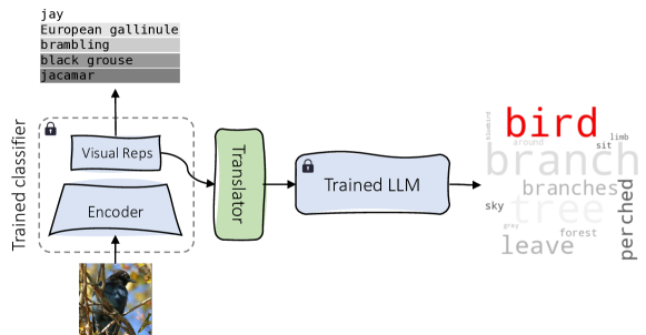
Figure 1: TExplain projects learned visual representations of a frozen image classifier onto a space that an independently trained language model can interpret. Using a large number of generated sentence samples along with the visual representation, TExplain produces a word cloud for each visual representation. Blue and green refers to frozen and trainable parameters, respectively. The category of the feature representation is highlighted in red, while other captured features are shown in gray. The font size of each word indicates the strength of its corresponding feature.

To the best of our knowledge, this is the first work to present a technique to encode learned visual features to textual explanations. Our contributions are summarized as follows:

1. We introduce TExplain, a novel approach that utilizes language models to explain the learned features of independently trained and frozen image classifiers.

2. We demonstrate that by performing minor feature translation, it is possible to generate explanations for frozen image classifiers using pre-trained language models.

3. Through empirical analysis, we validate the effectiveness of TExplain in identifying spurious features within a specific class.

4. We illustrate the practical application of TExplain by showcasing how it can be leveraged to mitigate spurious correlations within a dataset.

2 Method

Our method aims to elucidate the characteristics of image classifiers by leveraging pre-trained language models. To accomplish this, our architecture comprises three key components: a pre-trained frozen image classifier, a trainable translator network, and a pre-trained language model. An overview of the pipeline is depicted in Figure 1. During the training phase, our approach involves training a translator network to establish a connection between the features of the frozen image classifier and the pre-trained frozen language model, utilizing pairs of (image, caption). This enables us, during the inference stage, to provide explanations regarding the learning process of the image classifier for a given image by extracting the most frequent words among all its corresponding explanatory sentences.

2.1 Pre-trained Image Classifier

The primary component of our approach is the image classifier whose features we aim to interpret.

The input to the classifier is image $I\in\mathbb{R}^{H\times W\times C}$ where $H$, $W$, and $C$ are height, width, and the number of channels of the input image, respectively. To obtain the feature $Z$ that we aim to interpret, we pass the image $I$ through the pretrained (frozen) image classifier $enc(.)$. The resulting embedding $Z$ is obtained as $Z=enc(I)$ which in our case is the penultimate layer (before the classification layer).

While the choice of image classifier can vary, we specifically consider ViT (Dosovitskiy et al., 2020) due to its widespread usage. ViT’s architecture allows for efficient processing of large-scale image datasets and robust feature extraction. It splits the image into $P$ patches, adds a learnable token to the patch or token embeddings, and produces a $(P+1)\times D$ matrix, where $D$ represents the embedding dimension of each token. Hence, in the case of ViT, the feature $Z$ can be expressed as $Z\in\mathbb{R}^{(P+1)\times D}$.

2.2 Training the Translator Network

The embedding $Z$ generated by the image encoder represents the key characteristics captured by the classifier from the input image. During inference, our goal is to interpret this feature vector. To achieve this, we aim to transform the representation into a human-understandable description using natural language. This involves mapping the embeddings generated by the classifier’s encoder to the embedding space of a language model.

Concretely, $Z$ is flattened into a 1-dimensional vector $Z_{in}\in\mathbb{R}^{1\times((P+1)*D)}$. This vector is then passed through a translator network, denoted as $t(\cdot)$, to obtain $Z_{mapped}=t(Z_{in})$. Here, $Z_{mapped}$ shares the same size as the input of the text decoder of the language model. The translator is the only component in our framework that requires training and has a simple linear multi-layer perceptron (MLP) architecture with batch normalization.

To train $t(\cdot)$, we utilize image-sentence pairs ($I,S$). $Z_{in}$ is calculated given $I$ as the input to the classifier, and $Z_{mapped}$ is learned by minimizing the language model loss. The language model loss is defined as the cross-entropy loss between $S_{gen}$ and the ground truth sentence $S$. To generate $S_{gen}$, $Z_{mapped}$ is passed to the decoder ($dec(\cdot)$) of a pre-trained frozen language model. $S_{gen}=dec(Z_{mapped})$.

Once the translator network is trained, during inference, $S_{gen}$ serves as an explanation of the visual embedding captured by the frozen image classifier. This sheds light on its underlying features and patterns.

2.3 Identifying Dominant Words by Sampling

To minimize potential noise and enhance the reliability of the generated sentences from the language model, we employ Nucleus Sampling (Holtzman et al., 2019). This technique allows us to sample a set of $N$ sentences, denoted as $\{S_{gen}^{i}\}_{i=1}^{N}$. By removing the less frequently occurring words, we construct a word cloud based on the dominant words extracted from the set of sentences $\{S_{gen}^{i}\}_{i=1}^{N}$. This word cloud visually represents the prominent features within the visual embedding of the frozen classifier. By focusing on these dominant words, we gain insights into the key characteristics and attributes captured by the classifier’s visual representation. The word cloud serves as a concise and informative summary of the significant features present in the embedding space of the image encoder. It worth noting that focusing on frequent dominant words reduces the effect of hallucinations (Maynez et al., 2020) imposed by language models, as those words appear in majority of the generated sentences given a feature vector.

3 Implementation details

Models. While we acknowledge that alternative variants of the main models can be substituted, we have chosen to employ widely recognized and popular models for the sake of simplicity. Specifically, we utilized the pretrained ViT-base model (Wu et al., 2020) as our image classifier. This model incorporated 577 tokens and processed input images at a resolution of $384\times 384$ pixels. For the language model, we utilized the pre-trained BERT-base model (Devlin et al., 2018), featuring 12 layers and 12 attention heads. Regarding the translator component, we utilize a straightforward architecture consisting of a three-layered linear MLP with batch normalization. In the case of ViT, its input size is $577\times 768$ and outputs the same dimension, which is then reshaped to match the input of $dec(\cdot)$.

Sampling Explanations. Using nucleus sampling, we sample 1000 sentences from each visual representation. Hence, when generating class-level explanations, we will have $N\times 1000$, where $N$ represents the number of samples in that class. To maintain coherence, we set the cumulative probability threshold to 0.95. Additionally, we define the minimum and maximum length of the generated sentences to be 20 and 30 words, respectively. This sampling strategy allows us to capture a range of explanations that effectively convey the salient features present in the visual representations.

Data. We used a comprehensive dataset comprising a total of 14 million data points. This dataset encompassed COCO (Lin et al., 2014) and Visual Genome (Krishna et al., 2017) which come with human annotations, as well as three web datasets, including Conceptual Captions and Conceptual 12M (Changpinyo et al., 2021), and SBU captions (Ordonez et al., 2011). We trained the translator using all the data, excluding the COCO dataset, for 20 epochs. Subsequently, we fine-tuned the translator using the COCO dataset for an additional 5 epochs. Throughout the training process, a batch size of 512 was employed.

4 Experiments

In this section, we present the experiments conducted to investigate the capabilities of TExplain, our proposed language model-based technique. We commence with a straightforward and intuitive experiment on an altered version of the Cats vs Dogs dataset (Elson et al., 2007), where our goal is to train an image encoder to learn co-occurring features within images. Through this experiment, we aim to evaluate the effectiveness of our TExplain in capturing relevant and meaningful information from the trained model. Subsequently, we delve into an analysis of shortcuts on the Background Challenge dataset (Xiao et al., 2020) and spurious correlations on the Waterbirds dataset (Sagawa et al., 2019) using TExplain as a means to mitigate these correlations.

4.1 Faithfulness Test 1: Verifying that TExplain Picks up Relevant Features

In this experiment, we assess an Imagenet classifier’s performance using images in which the foreground is hidden (Only-BG-T from the Background Challenge datastet). Our hypothesis is that if the classifier consistently assigns the same label to an image, regardless of whether the foreground is visible or concealed, it indicates the presence of potentially misleading correlations between different regions of the image and the classifier’s predictions. Consequently, the TExplain should effectively bring attention to these correlations. In Figure 2, we present samples from the Background challenge dataset, illustrating instances where the classifier consistently assigns the same label to the images, even when the foreground is concealed. To shed light on the underlying associations, we utilize TExplain to generate word clouds from frequent words for each sample. These word clouds effectively highlight the correlated shortcuts present in each image. For instance, we observe a notable co-occurrence of "smoke," "train," and "track," which the classifier relies on as shortcuts for the steam locomotive category. This visualization further emphasizes the classifier’s dependence on these spurious correlations that TExplain identifies.

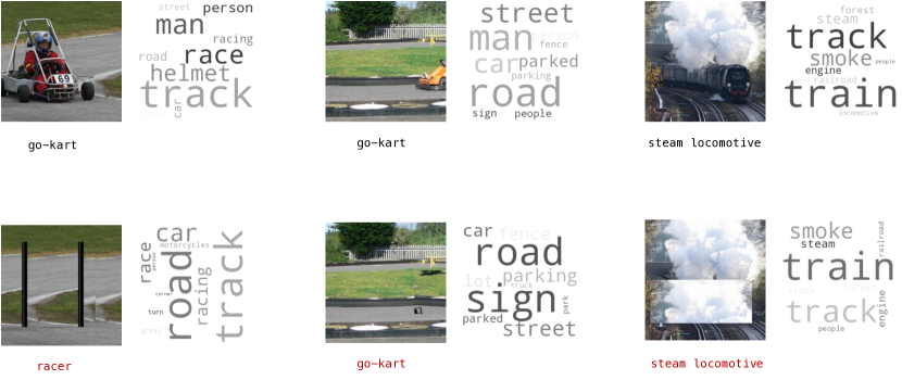
Figure 2: Class predictions and corresponding word clouds generated by TExplain for both the original (top) and Only-BG-T (bottom) samples extracted from the Background Challenge dataset. The class predictions are displayed below each image.

4.2 Faithfulness Test 2: Human Analysis

We conducted two separate human analysis experiments on three different from the background challenge (ImageNet-9) dataset: a) Raters were presented with a set of the 10 most frequent words produced by TExplain for each feature vector alongside the corresponding image. They were then asked to indicate how many words accurately matched the content of the image. b) In another experiment, raters were provided with the classifier’s top prediction for an image and the top word in the most frequent list generated by TExplain. Raters were instructed to determine the relevance of these two words, providing ’yes’ or ’no’ responses. The results of these experiments are illustrated in Figure 3. As depicted in Figure 3 (left), the raters consistently identified matching words with the image among the ten most frequent words. Similarly, Figure 3 (right) demonstrates that the classifier’s top prediction frequently aligns with the most frequent word generated by TExplain.

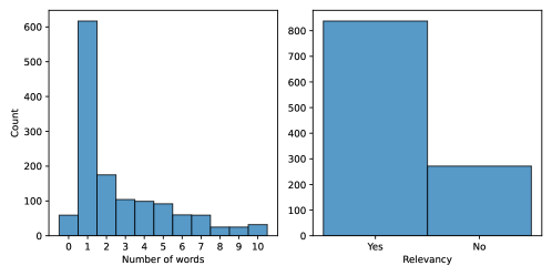
Figure 3: Human analysis experiments were conducted to validate that TExplain generates meaningful explanations. The left side shows the count of relevant words, while the right side illustrates whether the most frequent word produced by TExplain is relevant to the classifier’s top prediction.

4.3 Faithfulness Test 3: Verifying using Generative Model’s Latent Space

In this experiment, our goal is to assess the ability of the TExplain technique to emphasize prominent features within the latent space of Stable Diffusion (SD) (Rombach et al., 2022). Our rationale is based on the fact that SD generates an image from a latent vector, meaning this vector should encapsulate sufficient information to create a corresponding image. Our investigation aims to confirm the correlation between the textual features we extract from SD’s latent space (using TExplain) and the features that can be derived from the image using standard multi-modal models. To pinpoint the primary objects or features within the generated image, we utilize the BLIP method (Li et al., 2022) to generate descriptive captions for the output image. We expect our TExplain’s explanations within the latent space to align with BLIP-generated captions in the output space. To asses this we start by selecting a specific category, for example, "kitchen." Using corresponding category captions from the COCO dataset as prompts, we generate 100 images for each prompt using the SD model. At the same time, we employ BLIP to generate captions for these newly created images. During this process, we also extract latent features before generating each image. These latent features originate from the final step of the SD model, just before they are passed through the decoder of the variational auto-encoder to create an image. Subsequently, we take these latent features and process them through our TExplain model, resulting in explanations situated within the latent space.

We then proceed to create two word clouds for each category: one based on the image captions generated by BLIP and another derived from the latent space explanations produced by TExplain. In Figure 4, we present a visual comparison between the word clouds generated by BLIP (at the top) and those generated by TExplain (at the bottom) for three distinct categories, namely "kitchen," "bathroom," and "bus." As shown in the figure, the explanations provided by TExplain contains a similar distribution of objects and categories when compared to BLIP’s captions. This observation underscores the ability of TExplain to generate faithful explanations that align with the features present in the output space.’

We then extend this to 26 object categories and compute image captioning metrics such as ROUGE (Lin, 2004) and METEOR (Banerjee and Lavie, 2005), as well as cosine similarity between the sentence embeddings obtained using BERT for both TExplain and BLIP. We report these results in Table 1. Notably, the average cosine distance for TExplain and BLIP across all the categories is approximately 0.85, indicating that TExplain identifies learned features.

Table 1: Quantifying the relevancy of textual feature-based explanations by TExplain and image-based captions using BLIP.

	Cosine similarity	ROUGE	METEOR
Scores	0.845	40.39	38.95

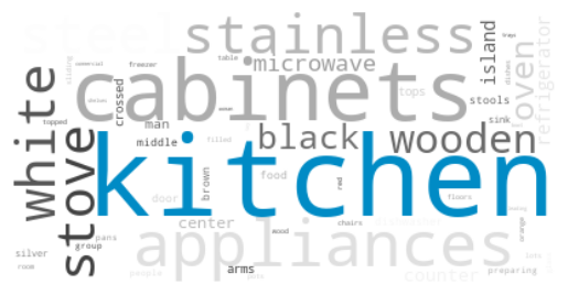
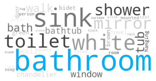
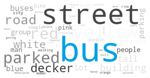
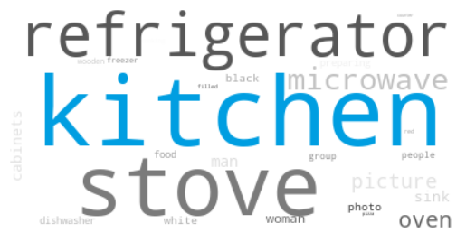
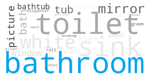
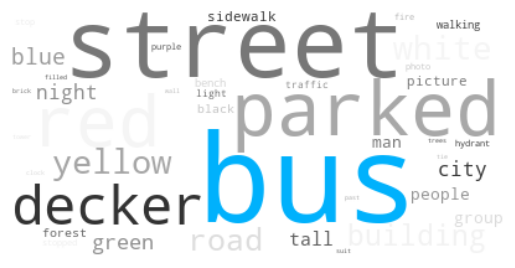
Figure 4: Wordclouds based on image captioning (top) with BLIP and feature captioning (bottom) using TExplain for categories kitchen, bathroom, and bus.

4.4 Detecting Potential Shortcuts/Spurious Correlations

ImageNet-9L. In an effort to extend our evaluation, we conducted a comprehensive analysis of TExplain using the Background Challenge dataset (Xiao et al., 2020). The Background Challenge dataset is publicly accessible and comprises test sets derived from ImageNet-9 (Deng et al., 2009), containing diverse foreground and background signals. Its primary objective is to assess the extent to which deep classifiers depend on irrelevant features for image classification.

To analyze the prominent features within each category of this dataset, we employed TExplain to generate word clouds for all categories. Figure 5 showcases the outcomes of this process. In the wheeled vehicle category, dominant features such as "street", "truck", and "car" emerged prominently. Conversely, in the fish category, the primary feature observed was "water", which exhibited an even stronger influence than the fish itself. These findings strongly indicate that the classifier is more likely to rely on shortcut features rather than the genuine object features.

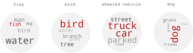
Figure 5: Word clouds generated from TExplain explanations for the Background Challenge Dataset categories. Red represents the detected features related to the main category.

To further investigate this observation, we conducted a detailed analysis using the Only-BG-T configuration from the dataset. In this configuration, the foreground is obscured with a portion of the background taken from the same image. As shown in Figure 6 (top), when the original images of a car and a bird are processed through the image classifier, the predicted ImageNet classes are mostly relevant to their respective categories. However, when the foreground is concealed, as illustrated in Figure 6 (bottom), the classifier still predicts bird and wheeled vehicle types. These findings corroborate the observations made in Figure 5. For instance, TExplain successfully detects "tree" and "branch" as dominant features for the bird category. When the bird is concealed, as shown in Figure 6 (bottom), the classifier tends to associate the remaining "branches" with the concept of a bird. Similarly, the car example in Figure 6 shows that "street" and "road" are correctly identified by TExplain in Figure 5.

TExplain not only exposes classifier bias, but it also has the potential to reveal dataset properties. For instance, in Figure 6, the prevalence of the man category for fish suggests that the dataset may contain many images of fishermen displaying their catches. Similarly, comparing the dog categories in the Background Challenge dataset indicates that the former likely has more outdoor images of dogs playing, as evidenced by the presence of grass and Frisbee, while the latter has more indoor images of dogs, indicated by the prominence of beds. Therefore, TExplain can serve as a tool for detecting bias in datasets and may provide insights on how to mitigate such biases by including samples from underrepresented classes to achieve balance.

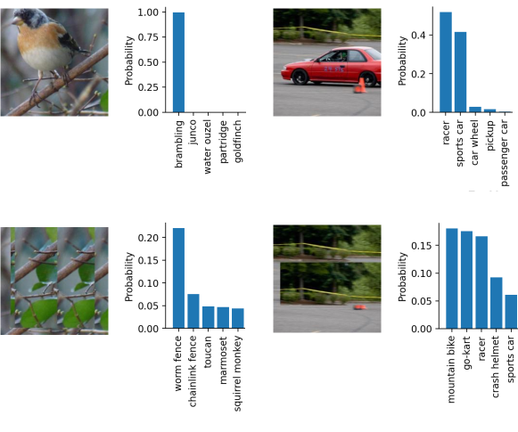
Figure 6: Top-5 class prediction probabilities on the original (top) and their corresponding Only-BG-T (bottom) samples from the ImageNet-9 dataset.

Waterbirds. The Waterbirds dataset, introduced by Sagawa et al. (Sagawa et al., 2019), serves as a benchmark for evaluating the extent to which models capture spurious correlations present in the training set. We employed TExplain to analyze both the training and test sets of each category, specifically the waterbirds and landbirds categories. As depicted in Figure 7, TExplain successfully identified significant shifts in the feature spaces between the training and test sets of each category. Notably, in the training set of the waterbirds class, the attribute "water" exhibited a much stronger presence compared to "bird", whereas in the waterbirds test set, these two features were more balanced. Additionally, in the test set of waterbirds, TExplain detected land attributes such as "grass", "tree", and "branch", which were not prominent in the training set of waterbirds. In essence, the waterbirds test set contained images of waterbirds on land, which the model had not encountered during training. It is worth noting that this subgroup (waterbirds on land) represents a particularly challenging category for most trained classifiers, as their performance tends to be subpar in such cases. Similarly, when examining the word clouds of the landbirds class, the attribute "water" became dominant in the test set compared to the training set of landbirds, where TExplain did not identify such an attribute.

Figure 7: Word clouds of the explanations generated by TExplain for the Waterbirds dataset. TExplain reveals significant feature shifts between the training and test sets within each category. Notably, in the training set of waterbirds, the attribute "water" outweighs "bird" in dominance compared to its respective test set. Additionally, the test set of landbirds exhibits the presence of "water" and "beach" attributes, which are absent in its corresponding training set.

Leveraging TExplain to Mitigate Spurious Correlations. In addition to visualizing and detecting potential spurious correlations and shortcuts learned by a model, TExplain can be utilized to enhance the model’s performance when encountering such correlations. In the case of the Waterbirds dataset, although most classifiers exhibit reasonable overall accuracy on the test set, their performance significantly deteriorates when evaluating specific subgroups. Our objective is to improve accuracy specifically for the worst-performing subgroup while maintaining a high average accuracy. To achieve this, we train classifier on the Waterbirds dataset and employ TExplain on the training set to identify the "problematic" samples. It is our assumption that the samples in which a class with a prominent presence other than the correct one is observed, are the instances in which the classifier is giving undue attention to the spurious features. Therefore, we select samples whose the first dominant feature is something other than "bird". By pinpointing these samples ($29\%$ of the training data), as done in (Asgari et al., 2022), we utilize GradCAM (Selvaraju et al., 2017) to localize and mask irrelevant areas (the first non-bird dominant feature that TExplain identifies) in the input. Subsequently, we fine-tune the trained model exclusively using the masked samples. The results presented in Table 2 demonstrate that employing TExplain yields a substantial improvement in the accuracy of the worst-performing subgroup while maintaining the average accuracy. Furthermore, in the second and third rows of the table, we compare this approach to randomly masking the training set, to match the number of samples identified as problematic by TExplain.

Table 2: Classification results from the Waterbirds dataset using ViT. Our method significantly improves empirical risk minimization (ERM)’s accuracy on the worst-group. Results are averaged over three different runs. In each run, TExplain demonstrated a substantial improvement in the ERM performance while outperforming other methods using significantly fewer masked samples during fine-tuning.

	ERM	RandMask	MaskTune	TExplain (ours)
Subgroup-1	98.20 $\pm$ 0.72	98.14 $\pm$ 1.76	97.63 $\pm$ 2.22	97.96 $\pm$ 0.25
Subgroup-2	89.49 $\pm$ 5.35	90.10 $\pm$ 2.80	93.62 $\pm$ 5.11	94.06 $\pm$ 1.82
Subgroup-3	97.95 $\pm$ 1.15	98.03 $\pm$ 1.97	97.96 $\pm$ 2.25	98.12 $\pm$ 0.47
Worst-group	89.79 $\pm$ 8.13	91.72 $\pm$ 2.49	95.195 $\pm$ 5.33	95.63 $\pm$ 2.55
Average	96.34 $\pm$ 2.12	96.59 $\pm$ 0.91	97.10 $\pm$ 0.71	97.39 $\pm$0.16
Masked Samples	N/A	100%	100%	26%

5 Related Work

Visual Heat Map-based Explanations.

A significant body of research has focused on post-hoc explanation techniques for image classifiers, including methods such as Grad-CAM (Selvaraju et al., 2017), LIME (Ribeiro et al., 2016), CAM (Wang et al., 2020), ablation studies (Ramaswamy et al., 2020), DeepLIFT (Collins et al., 2018), and saliency maps (Fong and Vedaldi, 2017). These methods typically rely on network gradients or perturbation analysis to generate heat maps that highlight the most relevant regions in an input image for the classifier’s decision. While these approaches effectively indicate the areas contributing to the classifier’s prediction, they lack the ability to provide a detailed understanding of the specific features learned by the model. Moreover, interpreting these heat maps can often be challenging and subjective. In contrast, our proposed approach leverages textual explanations to represent the learned features captured by the classifier, offering a more intuitive and direct interpretation of its decision-making process. By visualizing the dominant words, our method provides a comprehensive and accessible means to comprehend the underlying features encoded by the classifier, enabling a deeper understanding of its behavior and facilitating more informed analysis.

Textual Explanation of Vision Models.

Previous research has demonstrated the efficacy of incorporating textual explanations in training vision models, particularly in the context of multi-modal setups like visual question answering (Park et al., 2018; Sammani et al., 2022). Furthermore, the utilization of large-scale vision-language models in classification tasks has shown promising self-explanatory capabilities (Radford et al., 2021; Li et al., 2022, 2023; Jia et al., 2021; Singh et al., 2022). Notably, Menon and Vondrick (2022) recently proposed a technique to improve the interpretability of vision-language models used for image classification. However, the existing studies predominantly concentrate on elucidating vision-language models trained and fine-tuned jointly. There might be architectural similarities between our work and recent concurrent vision-language models such as (Li et al., 2023; Zhu et al., 2023; Liu et al., 2023). However, it is important to note that these models are designed for a different objective, such as image captioning, where a vision and a language model are trained together or individually. The exploration of interpreting the frozen embeddings of independently trained image classifiers using trained (and frozen) language models remains largely unexplored or deficient in current methodologies. This gap underscores the need for novel approaches that specifically address the challenge of interpreting independently trained image classifiers—an aspect that our proposed method aims to tackle.

6 Conclusion

We presented TExplain, a novel method that leverages the power of language models to interpret the learned features of independently trained image classifiers. Our approach enabled the generation of comprehensive textual explanations for learned visual features, revealing spurious correlations, biases, and uncovering underlying patterns. To validate the efficacy of TExplain, we conducted a series of experiments to ensure its proper functioning and reliability. We then demonstrated a practical application of the explanations that TExplain generates in identifying and mitigating spurious correlations ingrained within image classifiers. We uncovered and addressed these undesirable correlations, thereby enhancing the reliability and accuracy of the classifiers. This highlights the potential of TExplain as a valuable tool for finding and combating spurious correlations to promote more robust and trustworthy image classification models.

TExplain offers multiple applications in the realm of understanding and analyzing classifiers. Firstly, it can be employed to gain insights into the specific features that have been learned by a classifier. By generating comprehensive explanations, TExplain allows us to delve into the inner workings of the model and comprehend the learned representations. Secondly, it serves as a valuable tool for identifying biases and spurious correlations within the classifier. This capability enables the detection and mitigation of undesirable shortcuts or unintended associations that the model may have picked up during training. Lastly, TExplain can be utilized to assess data bias, assuming that the trained model itself is unbiased. By examining the generated explanations, we can gain valuable insights into any underlying biases present within the dataset being processed by the model. Overall, TExplain offers a versatile framework for uncovering and addressing various aspects of interpretability, bias, and feature analysis within classifiers.

In this paper we showed the application of TExplain on image classifiers and stable diffusion. An interesting avenue for future research is to explore its potential in other domains such as image segmentation and auto-encoders and other other architectures and input modalities. By adapting and applying TExplain to these contexts, we can gain valuable insights into the learned representations and underlying concepts within these models. Furthermore, it would be valuable to expand TExplain to encompass other data types, particularly in the realm of 3D (pointcloud, voxel, etc.) classifiers. One commonly held belief is that 3D data can inherently lead to capturing geometric information. Therefore, leveraging TExplain to investigate whether 3D encoders indeed extract geometry-related features could provide valuable insights into the learning process of these models. In this work, we performed multiple checks to ensure the explanation is indeed relevant to the learned visual features. However, we encourage using the method with even more checks to ensure that potentially learned biases from language models do not contribute to the final explanation.

References

- Adebayo et al. (2018) Julius Adebayo, Justin Gilmer, Michael Muelly, Ian Goodfellow, Moritz Hardt, and Been Kim. Sanity checks for saliency maps. Advances in neural information processing systems, 31, 2018.
- Alqaraawi et al. (2020) Ahmed Alqaraawi, Martin Schuessler, Philipp Weiß, Enrico Costanza, and Nadia Berthouze. Evaluating saliency map explanations for convolutional neural networks: a user study. In Proceedings of the 25th International Conference on Intelligent User Interfaces, pages 275–285, 2020.
- Asgari et al. (2022) Saeid Asgari, Aliasghar Khani, Fereshte Khani, Ali Gholami, Linh Tran, Ali Mahdavi Amiri, and Ghassan Hamarneh. Masktune: Mitigating spurious correlations by forcing to explore. Advances in Neural Information Processing Systems, 35:23284–23296, 2022.
- Banerjee and Lavie (2005) Satanjeev Banerjee and Alon Lavie. Meteor: An automatic metric for mt evaluation with improved correlation with human judgments. In Proceedings of the acl workshop on intrinsic and extrinsic evaluation measures for machine translation and/or summarization, pages 65–72, 2005.
- Brown et al. (2020) Tom Brown, Benjamin Mann, Nick Ryder, Melanie Subbiah, Jared D Kaplan, Prafulla Dhariwal, Arvind Neelakantan, Pranav Shyam, Girish Sastry, Amanda Askell, et al. Language models are few-shot learners. Advances in neural information processing systems, 33:1877–1901, 2020.
- Changpinyo et al. (2021) Soravit Changpinyo, Piyush Sharma, Nan Ding, and Radu Soricut. Conceptual 12m: Pushing web-scale image-text pre-training to recognize long-tail visual concepts. In Proceedings of the IEEE/CVF Conference on Computer Vision and Pattern Recognition, pages 3558–3568, 2021.
- Chu et al. (2020) Eric Chu, Deb Roy, and Jacob Andreas. Are visual explanations useful? a case study in model-in-the-loop prediction. arXiv preprint arXiv:2007.12248, 2020.
- Collins et al. (2018) Edo Collins, Radhakrishna Achanta, and Sabine Susstrunk. Deep feature factorization for concept discovery. In Proceedings of the European Conference on Computer Vision (ECCV), pages 336–352, 2018.
- Deng et al. (2009) Jia Deng, Wei Dong, Richard Socher, Li-Jia Li, Kai Li, and Li Fei-Fei. Imagenet: A large-scale hierarchical image database. In 2009 IEEE conference on Computer Vision and Pattern Recognition, pages 248–255. Ieee, 2009.
- Devlin et al. (2018) Jacob Devlin, Ming-Wei Chang, Kenton Lee, and Kristina Toutanova. Bert: Pre-training of deep bidirectional transformers for language understanding. arXiv preprint arXiv:1810.04805, 2018.
- Dosovitskiy et al. (2020) Alexey Dosovitskiy, Lucas Beyer, Alexander Kolesnikov, Dirk Weissenborn, Xiaohua Zhai, Thomas Unterthiner, Mostafa Dehghani, Matthias Minderer, Georg Heigold, Sylvain Gelly, et al. An image is worth 16x16 words: Transformers for image recognition at scale. arXiv preprint arXiv:2010.11929, 2020.
- Elson et al. (2007) Jeremy Elson, John R Douceur, Jon Howell, and Jared Saul. Asirra: a captcha that exploits interest-aligned manual image categorization. CCS, 7:366–374, 2007.
- Fong and Vedaldi (2017) Ruth C Fong and Andrea Vedaldi. Interpretable explanations of black boxes by meaningful perturbation. In Proceedings of the IEEE international conference on computer vision, pages 3429–3437, 2017.
- Holtzman et al. (2019) Ari Holtzman, Jan Buys, Li Du, Maxwell Forbes, and Yejin Choi. The curious case of neural text degeneration. arXiv preprint arXiv:1904.09751, 2019.
- Jia et al. (2021) Chao Jia, Yinfei Yang, Ye Xia, Yi-Ting Chen, Zarana Parekh, Hieu Pham, Quoc Le, Yun-Hsuan Sung, Zhen Li, and Tom Duerig. Scaling up visual and vision-language representation learning with noisy text supervision. In International Conference on Machine Learning, pages 4904–4916. PMLR, 2021.
- Kindermans et al. (2019) Pieter-Jan Kindermans, Sara Hooker, Julius Adebayo, Maximilian Alber, Kristof T Schütt, Sven Dähne, Dumitru Erhan, and Been Kim. The (un) reliability of saliency methods. Explainable AI: Interpreting, explaining and visualizing deep learning, pages 267–280, 2019.
- Krishna et al. (2017) Ranjay Krishna, Yuke Zhu, Oliver Groth, Justin Johnson, Kenji Hata, Joshua Kravitz, Stephanie Chen, Yannis Kalantidis, Li-Jia Li, David A Shamma, et al. Visual genome: Connecting language and vision using crowdsourced dense image annotations. International journal of computer vision, 123:32–73, 2017.
- Li et al. (2022) Junnan Li, Dongxu Li, Caiming Xiong, and Steven Hoi. Blip: Bootstrapping language-image pre-training for unified vision-language understanding and generation. In International Conference on Machine Learning, pages 12888–12900. PMLR, 2022.
- Li et al. (2023) Junnan Li, Dongxu Li, Silvio Savarese, and Steven Hoi. Blip-2: Bootstrapping language-image pre-training with frozen image encoders and large language models. arXiv preprint arXiv:2301.12597, 2023.
- Lin (2004) Chin-Yew Lin. Rouge: A package for automatic evaluation of summaries. In Text summarization branches out, pages 74–81, 2004.
- Lin et al. (2014) Tsung-Yi Lin, Michael Maire, Serge Belongie, James Hays, Pietro Perona, Deva Ramanan, Piotr Dollár, and C Lawrence Zitnick. Microsoft coco: Common objects in context. In Computer Vision–ECCV 2014: 13th European Conference, Zurich, Switzerland, September 6-12, 2014, Proceedings, Part V 13, pages 740–755. Springer, 2014.
- Liu et al. (2023) Haotian Liu, Chunyuan Li, Qingyang Wu, and Yong Jae Lee. Visual instruction tuning. arXiv preprint arXiv:2304.08485, 2023.
- Maynez et al. (2020) Joshua Maynez, Shashi Narayan, Bernd Bohnet, and Ryan McDonald. On faithfulness and factuality in abstractive summarization. arXiv preprint arXiv:2005.00661, 2020.
- Menon and Vondrick (2022) Sachit Menon and Carl Vondrick. Visual classification via description from large language models. arXiv preprint arXiv:2210.07183, 2022.
- Ordonez et al. (2011) Vicente Ordonez, Girish Kulkarni, and Tamara Berg. Im2text: Describing images using 1 million captioned photographs. Advances in neural information processing systems, 24, 2011.
- Park et al. (2018) Dong Huk Park, Lisa Anne Hendricks, Zeynep Akata, Anna Rohrbach, Bernt Schiele, Trevor Darrell, and Marcus Rohrbach. Multimodal explanations: Justifying decisions and pointing to the evidence. In Proceedings of the IEEE conference on computer vision and pattern recognition, pages 8779–8788, 2018.
- Poursabzi-Sangdeh et al. (2021) Forough Poursabzi-Sangdeh, Daniel G Goldstein, Jake M Hofman, Jennifer Wortman Wortman Vaughan, and Hanna Wallach. Manipulating and measuring model interpretability. In Proceedings of the 2021 CHI conference on human factors in computing systems, pages 1–52, 2021.
- Radford et al. (2021) Alec Radford, Jong Wook Kim, Chris Hallacy, Aditya Ramesh, Gabriel Goh, Sandhini Agarwal, Girish Sastry, Amanda Askell, Pamela Mishkin, Jack Clark, et al. Learning transferable visual models from natural language supervision. In International conference on machine learning, pages 8748–8763. PMLR, 2021.
- Ramaswamy et al. (2020) Harish Guruprasad Ramaswamy et al. Ablation-cam: Visual explanations for deep convolutional network via gradient-free localization. In Proceedings of the IEEE/CVF Winter Conference on Applications of Computer Vision, pages 983–991, 2020.
- Ribeiro et al. (2016) Marco Tulio Ribeiro, Sameer Singh, and Carlos Guestrin. " why should i trust you?" explaining the predictions of any classifier. In Proceedings of the 22nd ACM SIGKDD international conference on knowledge discovery and data mining, pages 1135–1144, 2016.
- Rombach et al. (2022) Robin Rombach, Andreas Blattmann, Dominik Lorenz, Patrick Esser, and Björn Ommer. High-resolution image synthesis with latent diffusion models. In Proceedings of the IEEE/CVF conference on computer vision and pattern recognition, pages 10684–10695, 2022.
- Sagawa et al. (2019) Shiori Sagawa, Pang Wei Koh, Tatsunori B Hashimoto, and Percy Liang. Distributionally robust neural networks for group shifts: On the importance of regularization for worst-case generalization. arXiv preprint arXiv:1911.08731, 2019.
- Sammani et al. (2022) Fawaz Sammani, Tanmoy Mukherjee, and Nikos Deligiannis. Nlx-gpt: A model for natural language explanations in vision and vision-language tasks. In Proceedings of the IEEE/CVF Conference on Computer Vision and Pattern Recognition, pages 8322–8332, 2022.
- Selvaraju et al. (2017) Ramprasaath R Selvaraju, Michael Cogswell, Abhishek Das, Ramakrishna Vedantam, Devi Parikh, and Dhruv Batra. Grad-cam: Visual explanations from deep networks via gradient-based localization. In Proceedings of the IEEE International Conference on Computer Vision, pages 618–626, 2017.
- Singh et al. (2022) Amanpreet Singh, Ronghang Hu, Vedanuj Goswami, Guillaume Couairon, Wojciech Galuba, Marcus Rohrbach, and Douwe Kiela. Flava: A foundational language and vision alignment model. In Proceedings of the IEEE/CVF Conference on Computer Vision and Pattern Recognition, pages 15638–15650, 2022.
- Srinivas and Fleuret (2020) Suraj Srinivas and François Fleuret. Rethinking the role of gradient-based attribution methods for model interpretability. arXiv preprint arXiv:2006.09128, 2020.
- Vaswani et al. (2017) Ashish Vaswani, Noam Shazeer, Niki Parmar, Jakob Uszkoreit, Llion Jones, Aidan N Gomez, Łukasz Kaiser, and Illia Polosukhin. Attention is all you need. Advances in neural information processing systems, 30, 2017.
- Wang et al. (2020) Haofan Wang, Zifan Wang, Mengnan Du, Fan Yang, Zijian Zhang, Sirui Ding, Piotr Mardziel, and Xia Hu. Score-cam: Score-weighted visual explanations for convolutional neural networks. In Proceedings of the IEEE/CVF conference on computer vision and pattern recognition workshops, pages 24–25, 2020.
- Wu et al. (2020) Bichen Wu, Chenfeng Xu, Xiaoliang Dai, Alvin Wan, Peizhao Zhang, Zhicheng Yan, Masayoshi Tomizuka, Joseph Gonzalez, Kurt Keutzer, and Peter Vajda. Visual transformers: Token-based image representation and processing for computer vision. arXiv preprint arXiv:2006.03677, 2020.
- Xiao et al. (2020) Kai Xiao, Logan Engstrom, Andrew Ilyas, and Aleksander Madry. Noise or signal: The role of image backgrounds in object recognition. arXiv preprint arXiv:2006.09994, 2020.
- Zhu et al. (2023) Deyao Zhu, Jun Chen, Xiaoqian Shen, Xiang Li, and Mohamed Elhoseiny. Minigpt-4: Enhancing vision-language understanding with advanced large language models. arXiv preprint arXiv:2304.10592, 2023.