A Semi-classical Spacetime Region with Maximum Entropy

Abstract

We consider a 4D spherically-symmetric static finite spacetime region as a collection of quanta in the semi-classical Einstein equation and study the entropy including the self-gravity. For sufficiently excited states, we estimate the entropy in a WKB-like method considering local consistency with thermodynamics and find its upper bound. The saturation condition uniquely determines the entropy-maximized spacetime as a radially uniform dense configuration with near-Planckian curvatures and a surface just outside the Schwarzschild radius. The interior metric is a non-perturbative solution in $\hbar$, leading to the species bound. The maximum entropy then saturates the Bousso bound and coincides with the Bekenstein-Hawking formula. Thus, the Bousso bound in this class of spacetime is verified by constructing the saturating configuration that has no horizon and stores information inside.

I Introduction

An interesting question, in which quantum theory, gravity, and thermodynamics are closely intertwined, is “What is the maximum entropy that can be given to a finite region?”, which should play a key role in searching for the fundamental degrees of freedom of quantum gravity tHooft ; Susskind ; Smolin ; Bousso2 . For this, the Bekenstein bound Bek_bound and the Bousso bound Bousso1 have been conjectured, and the existence of a horizon saturates both bounds. However, this is just a sufficient condition for the saturation, and the necessary one, or more physically, the spacetime structure that maximizes entropy, has not been well investigated. In this paper, we attempt to find it in a certain class of spacetime.

Then, self-gravity must be taken into account. This is because thermodynamic entropy depends on gravity. Suppose that we have a spherical static region with size $R$ and finite energy-momentum distribution, and the self-gravity is described by the metric $g_{\mu\nu}$ consistent with the Einstein equation. The outside is almost vacuum, and thus the boundary at $r=R$ plays a role of the surface of the region (see the left of Fig.1). We set the entropy of the region as

$$S=\int_{\Sigma}d\Sigma_{\mu}s^{\mu}=\int^{R}_{0}dr\sqrt{g_{rr}(r)}s(r),$$ (1)

with the conserved entropy current $s^{\mu}$, where $\Sigma$ is chosen as a spacelike hypersurface orthogonal to the timelike Killing vector foot:s_den . Here, the entropy density per proper radial length, $s(r)$, depends on the local temperature, which is $\frac{T_{global}}{\sqrt{-g_{tt}(r)}}$ if Tolman’s law holds Landau_SM ; Tolman . (1) also contains the effect of the proper length, $\sqrt{g_{rr}(r)}$. Thus, the self-gravity $g_{\mu\nu}$ makes the region inhomogeneous, breaking the extensivity of thermodynamic quantities, so that entropy follows not the volume law but another law that depends on $g_{\mu\nu}$. Indeed, the entropy of spherical self-gravitating thermal radiation behaves like $\sim R^{\frac{3}{2}}$ not $\sim R^{3}$ Sorkin (see Appendix A for a review).

Let us now speculate the microscopic meaning of the entropy in the semi-classical Einstein equation

$$G_{\mu\nu}=8\pi G\langle\psi|T_{\mu\nu}|\psi\rangle.$$ (2)

In a theory of many local degrees of freedom with local interactions, the static region is described as a collection of excited quanta according to an excited state $|\psi\rangle$ satisfying (2), where the static self-gravity $g_{\mu\nu}$ is determined self-consistently. See Fig.1.

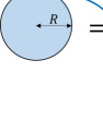
Figure 1: A semi-classical region with size $R$ as a collection of excited quanta in $(g_{\mu\nu},|\psi\rangle$) satisfying (2).

If sufficiently excited, the characteristic wavelength of the quanta around a point should be shorter than the radius of curvature of the spacetime there. In the region of about the wavelength, the effect of gravity is negligible, and the density of states should be high, consistent with thermodynamics Landau_SM . Then, there should exist many typical states $\{|\psi\rangle\}$ Goldstein ; Popescu ; Sugita ; Reimann that have, at a resolution about the wavelength, the same energy-momentum distribution and thus through (2) the same geometry $g_{\mu\nu}$. Therefore, the entropy $S$ should be given by the logarithm of the number of the typical states $\{|\psi\rangle\}$ that satisfy (2) for such a coarse-grained metric $g_{\mu\nu}$: $S[g_{\mu\nu}]$.

In this paper, we provide a primitive realization of this idea and find explicitly the spacetime $g_{\mu\nu}^{*}$ that maximizes the entropy inside $r=R$ in a class of 4D spherically-symmetric static spacetime: $S\leq S_{max}\equiv S[g_{\mu\nu}^{*}]$. Here, $X_{*}$ (or $X^{*}$) denotes a quantity $X$ for the entropy-maximized configuration.

As a first attempt, we estimate the order of the entropy $S[g_{\mu\nu}]$ including self-gravity $g_{\mu\nu}$ in a WKB-like/semi-classical method by focusing on sufficiently excited states $|\psi\rangle$ and assuming the phenomenological form (1) Francesco ; Landau_SM ; Zubarev (Sec.II). The key idea is to consider the quasi-local distribution of excited quanta with 1-bit of information about $|\psi\rangle$ consistent locally with thermodynamics, where the non-locality of entropy BFM ; BCFM is taken into account at a leading order in the WKB approximation. The self-gravity is introduced through the Hamiltonian constraint. The obtained entropy $S[g_{\mu\nu}]$ shows that the entropy is maximized by maximizing the typical excitation energy of the quanta at each $r$.

Then, an upper bound on the entropy emerges from a semi-classical inequality required by the global static condition: the global existence of the timelike Killing vector (Sec.III). The bound also leads to the Bekenstein bound including self-gravity. Note here that our class of spacetime has no trapped surface, since the Killing vector would become spacelike inside a trapped surface.

Next, we find the entropy-maximized configuration (Sec.IV). Assuming that the maximum excitation energy for the quantum is close to but smaller than the Planck energy, the condition saturating the entropy bound leads to uniquely an energy density meaning that the quanta are distributed uniformly in the radial direction (Sec.IV.1). This derivation and Appendix B show that a necessary and sufficient condition for the maximum entropy is the radial uniformity.

Then, the consistency with thermodynamics and semi-classicality determines uniquely the metric $g_{\mu\nu}^{*}$ (Sec.IV.2). We can check that if there are many local degrees of freedom, $g_{\mu\nu}^{*}$ is a non-perturbative self-consistent solution of (2) in $\hbar$, leading to the species bound Dvali1 ; Dvali2 . Note that $g_{\mu\nu}^{*}$ is robust in that it can be obtained in various approaches KMY ; KY1 ; KY2 ; Ho ; KY3 ; KY4 ; KY5 ; Y1 ; HKLY .

Geometrically, $g_{\mu\nu}^{*}$ is a warped product of $AdS_{2}$ with a near-Planckian radius and $S^{2}$ with radius $r$. Physically, $g_{\mu\nu}^{*}$ represents a dense configuration with near-Planckian curvature as Fig.4 (Sec.IV.3). The high curvature induces quantum fluctuations of various modes, generating a large quantum pressure that supports the system from strong gravity and self-consistently keeps the curvature large but finite. As a result, the energy is distributed throughout the interior, the central region is nearly flat, and no singularities appear. $g_{\mu\nu}^{*}$ is connected smoothly to the Schwarzschild metric with ADM mass $M_{0}\equiv\frac{a_{0}}{2G}~{}(\gg m_{p}\equiv\sqrt{\hbar/G})$, at the surface located at $r=R=a_{0}+\mathcal{O}\left(\frac{l_{p}^{2}}{a_{0}}\right)>a_{0}$. Therefore, there is no horizon while the information is kept inside for a long time due to a large redshift factor.

To evaluate explicitly $S[g_{\mu\nu}^{*}]=S_{max}$, we apply locally the Unruh effect (or the local temperature due to particle creation inside) and thermodynamic relations in $g_{\mu\nu}^{*}$ (Sec.V). We then find

$$S\leq S_{max}=\frac{\mathcal{A}}{4l_{p}^{2}},$$ (3)

where ${\cal A}\equiv 4\pi R^{2}=4\pi a_{0}^{2}+\mathcal{O}(1)$. Therefore, the maximum entropy $S_{max}$ coincides with the Bekenstein-Hawking formula, as a result of the strong self-gravity satisfying (2). The particle creation inside equilibrates the configuration in a heat bath at Hawking temperature and evaporates it in the vacuum.

Furthermore, we can apply $\nabla_{\mu}s^{\mu}=0$ and a regularity condition to all the configurations in our class and show that (1) agrees with one evaluated on a light-sheet $\Sigma$ introduced in Bousso1 and thus is covariant (Sec.VI.1). Therefore, (3) means that the entropy-maximized configuration, having no horizon, saturates the Bousso bound. Interestingly, $g_{\mu\nu}^{*}$ also saturates the local sufficient conditions proposed in FMW ; BFM for the Bousso bound (Sec.VI.2). Thus, the Bousso bound in this class of spacetime is verified by directly incorporating self-gravity and explicitly constructing the required configuration as the necessary condition for the saturation.

Finally, based on this entropy-maximized configuration with strong self-gravity and large quantum effect, we will discuss new ways to explore the meaning of the holographic principle (Sec.VII).

II Estimation of entropy $S[g_{\mu\nu}]$

We estimate entropy including self-gravity in a WKB-like manner and realize, at that level, the idea of $S[g_{\mu\nu}]$ mentioned in Sec.I. Generically, a quantum cannot simply be treated like a point particle because of its spread and entanglement, which leads to the non-locality of entropy BFM ; BCFM . If sufficiently excited, however, it behaves like a “particle” with a short wavelength and as localized as possible, corresponding to the leading solution of the WKB approximation. Then, a notion of the number of quanta can be introduced to estimate the entropy in a semi-classical way consistent locally with thermodynamics Landau_SM . We finally incorporate the self-gravity by Hamiltonian constraint and obtain the order of $S[g_{\mu\nu}]$.

II.1 1-bit quantum

We develop a self-consistent argument. Suppose that a spherically-symmetric static configuration of size $R$, consisting of a collection of many quanta in an excited state $|\psi\rangle$ like Fig.1, has the metric (for $r\leq R$)

$$ds^{2}=-\left(1-\frac{a(r)}{r}\right)e^{A(r)}dt^{2}+\left(1-\frac{a(r)}{r}\right)^{-1}dr^{2}+r^{2}d\Omega^{2}$$ (4)

and the energy-momentum distribution $\langle\psi|T_{\mu\nu}(r)|\psi\rangle$ satisfying (2). Here, $\frac{a(r)}{2G}$ is the Misner-Sharp mass inside $r$ Hayward . On the other hand, the region for $r\geq R$ is almost vacuum and can be approximated by the Schwarzschild metric with the ADM energy $M_{0}\equiv\frac{a_{0}}{2G}\approx\frac{a(R)}{2G}$. (See Appendix C for an example of the evaluation of $\langle\psi|T_{\mu\nu}(r)|\psi\rangle$ and its self-consistency.)

Each excited quantum at $r~{}(\leq R)$ may be in motion (in particular for a massless field), but from the spherically-symmetric static condition, spherically and time averaged, the quantum is stationary with respect to the timelike Killing vector $\partial_{t}$ and has the characteristic excitation energy, $\epsilon(r)(>0)$, measured locally. Here, we take as $\epsilon(r)$ the smallest excitation energy among the excited quanta that contribute significantly to representing the properties at $r$ inherent to the state $|\psi\rangle$ and determining the entropy BFM ; BCFM . In this sense, a quantum with $\epsilon(r)$ corresponds to the smallest unit in $|\psi\rangle$.

If $|\psi\rangle$ is sufficiently excited, a quantum around $r$ with $\epsilon(r)$ has a short wavelength such that

$$\lambda(r)\sim\frac{\hbar}{\epsilon(r)}\lesssim\mathcal{R}(r)^{-\frac{1}{2}},$$ (5)

and behaves like a “particle” with feeling little gravity, corresponding to the leading solution of the WKB approximation. Here, $\mathcal{R}(r)$ denotes the order of the magnitude of the curvatures of the metric (4). Then, if many such quanta are excited, according to thermodynamic typicality Goldstein ; Popescu ; Sugita ; Reimann , they typically behave like a local equilibrium state, at least, within a spherical subsystem at each $r$ in Fig.2. (Note that we don’t consider only configurations that are in local equilibrium in the strict sense, such as those corresponding to local Gibbs states Zubarev ; foot:Tolman .) Thus, $\epsilon(r)$ can be estimated by the local temperature $T_{loc}(r)$:

$$\epsilon(r)\sim T_{loc}(r),$$ (6)

which is determined self-consistently by $(g_{\mu\nu},|\psi\rangle)$ (see Appendix A and Sec.V.1 for examples). Here, from thermodynamic relation $T=\frac{dE}{dS}$, temperature $T$ is generally the typical energy per 1-bit of information demon . Therefore, a quantum with $\epsilon(r)$ has 1-bit of information around $r$ about the state $|\psi\rangle$, which is consistent with the definition of $\epsilon(r)$ above (see below for a further discussion). We call such a quantum a 1-bit quantum.

We also assume that the state $|\psi\rangle$ is excited enough to exceed the (possible) negative energy contribution from vacuum fluctuations BD , making the total energy density positive: $\langle\psi|-T^{t}{}_{t}(r)|\psi\rangle>0$.

II.2 Quasi-local distribution of information $N(r)$

To estimate the entropy of the system, we introduce an auxiliary function $N(r)$ taking into account the non-locality of entropy. We first divide the system into the smallest spherical unit in which the properties of $|\psi\rangle$ appear, i.e., spherical subsystems with width $\Delta\hat{r}\sim\lambda(r)$. See Fig.2.

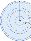
Figure 2: Decomposition of the region into spherical subsystems with width $\Delta\hat{r}\sim\lambda(r)$.

Here, $(\hat{t},\hat{r})$ is the local coordinate around $r$ with $\Delta\hat{t}=\sqrt{-g_{tt}(r)}\Delta t$ and $\Delta\hat{r}=\sqrt{g_{rr}(r)}\Delta r$. Each subsystem has the local energy $4\pi r^{2}\langle T^{\hat{t}\hat{t}}(r)\rangle\Delta\hat{r}=4\pi r^{2}\langle-T^{t}{}_{t}(r)\rangle\Delta\hat{r}$, where we use $g^{\hat{t}\hat{t}}=-1$ and $T^{t}{}_{t}=T^{\hat{t}}{}_{\hat{t}}=-T^{\hat{t}\hat{t}}$. Therefore,

$$N(r)\equiv\frac{4\pi r^{2}\langle-T^{t}{}_{t}(r)\rangle\Delta\hat{r}}{\epsilon(r)}~{}~{}~{}{\rm for}~{}~{}\Delta\hat{r}\sim\lambda(r)$$ (7)

estimates the order of the number of the 1-bit quanta within the subsystem. Here, quanta with excitation energies larger than $\epsilon(r)$ can also be included in this subsystem and contribute to $4\pi r^{2}\langle-T^{t}{}_{t}(r)\rangle\Delta\hat{r}$, and we consider them as combinations of the 1-bit quanta. For the semi-classical estimation Landau_SM , we assume

$$N(r)\gg 1,$$ (8)

which should hold if many degrees of freedom are sufficiently excited. Then, the subsystem has $\mathcal{O}(N(r))$ bit of entropy, since a 1-bit quantum typically has 1-bit of entropy. Thus, there exist $\mathcal{O}(e^{N(r)})$ typical states that can represent the subsystem with the same energy distribution $\langle T_{\mu\nu}(r)\rangle$ at the resolution of $\Delta\hat{r}\sim\lambda(r)$.

This estimation can also be obtained in a different manner inspired by Bekenstein’s thought experiment Bekenstein . In general, a localized quantum of wavelength $\lambda$ has 1 bit of information about whether it exists in a “box” of size $\sim\lambda$: at a resolution of about $\lambda$, it exists with almost half probability and does not exist with almost half probability. Thus, such a quantum is most uncertain about its existence at almost the same resolution as its wavelength, which means that the region occupied by the quantum has the corresponding 1-bit of information. Now, applying this idea to our subsystem at $r$, which contains $\mathcal{O}(N(r))$ 1-bit quanta and has almost the same width as that of the quanta, there exist $\mathcal{O}(2^{N(r)})$ different patterns for whether the quanta are present there. Therefore, the subsystem has $\mathcal{O}(N(r))$ bits of information about how it constitutes itself microscopically.

Thus, we use $N(r)$ to estimate the entropy density per proper radial length in the WKB-like approach as

$$s(r)=\frac{N(r)}{\Delta\hat{r}}~{}~{}~{}{\rm for}~{}~{}\Delta\hat{r}\sim\lambda(r).$$ (9)

This and (7) lead to the relations:

$$\langle-T^{t}{}_{t}(r)\rangle \sim\frac{N(r)\epsilon(r)^{2}}{4\pi\hbar r^{2}},~{}~{}s(r)\sim\frac{N(r)\epsilon(r)}{\hbar},$$ (10)

$$s(r) =\frac{4\pi r^{2}\langle-T^{t}{}_{t}(r)\rangle}{\epsilon(r)},$$ (11)

which hold for typical states.

This is consistent with thermodynamics. Indeed, for a highly excited state that macroscopically behaves like a ultra-relativistic fluid (including self-gravity), the Stefan-Boltzmann law holds approximately, leading to Landau_SM ; fluidbook

$$\frac{s(r)}{4\pi r^{2}}=\frac{4\langle-T^{t}{}_{t}(r)\rangle}{3T_{loc}(r)}.$$ (12)

Therefore, (11) and (12) are consistent through (6). (See Appendix A for more consistencies.)

We here see the properties of $N(r)$. First, $N(r)$ is quasi-local in the sense that it is defined only at resolutions of width $\Delta\hat{r}\sim\lambda(r)$, which accounts for the non-locality of entropy BFM ; BCFM . Also, $N(r)$ is covariant in that the quanta are stationary with respect to the timelike Killing vector, a covariant notion (see also Sec.VI).

II.3 Self-gravity

Now, we estimate the total entropy (1) considering self-gravity. The Hamiltonian constraint $\mathcal{H}=0$ ($G_{tt}=8\pi G\langle T_{tt}\rangle$) plays the key role:

$$\partial_{r}a(r)=8\pi Gr^{2}\langle-T^{t}{}_{t}(r)\rangle,$$ (13)

which gives Poisson ; Sorkin ; Landau_CF

$$\frac{a(r)}{2G}=4\pi\int^{r}_{0}dr^{\prime}r^{\prime 2}\langle-T^{t}{}_{t}(r^{\prime})\rangle.$$ (14)

From this, (4) and (10), (1) can be estimated as

$$S\sim\frac{1}{\hbar}\int^{R}_{0}drN(r)\epsilon(r)\left(1-\frac{2}{r}\int^{r}_{0}dr^{\prime}N(r^{\prime})\frac{\epsilon(r^{\prime})^{2}}{m_{p}^{2}}\right)^{-\frac{1}{2}}.$$ (15)

This provides what should be considered as the entropy $S[g_{\mu\nu}]$ for the self-consistent solution to (2).

(15) shows that for a given $N(r)$, the largest $\epsilon(r)$ leads to the largest $S$. More precisely, according to the second law within each spherical subsystem, the entropy density $\frac{s(r)}{4\pi r^{2}}\sim\frac{N(r)\epsilon(r)}{4\pi\hbar r^{2}}$ (from (10)) should be an increasing function of the local temperature $T_{loc}(r)$ Landau_SM , and thus the maximum local temperature at each $r$ provides the maximum entropy $S_{max}$ for a given size $R$. This is consistent with ordinary thermodynamic behavior without self-gravity Landau_SM , but it is a non-trivial result because self-gravity is included here.

In order for the semi-classical description to be valid, the excitation energy $\epsilon(r)$ of a 1-bit quantum (or the local temperature $T_{loc}(r)$ from (6)) should satisfy Pad_Lim ; Caianiello ; Brandt

$$\epsilon(r)\leq\epsilon_{max}\sim\frac{m_{p}}{\sqrt{n}}$$ (16)

with $n\gg 1$, a large number of $\mathcal{O}(1)$. Here, $\mathcal{O}(1)$ means $\mathcal{O}(r^{0})$ or $\mathcal{O}(a^{0}_{0})$ for $r,a_{0}\gg l_{p}$.

Here are some comments on the subtleties of the above entropy evaluation. We use only the geometrical static condition and local consistencies with thermodynamics and do not assume a priori a global thermodynamic equilibrium. This is motivated by two facts. Physically, static configurations should be considered including their formation processes, and mechanical and global/local thermodynamic equilibria are generically different due to differences in relaxation time scales Landau_SM . Therefore, we need to consider in which equilibrium state the configuration is, depending on the time scale we are considering. The other is that, a notion of global thermodynamic equilibrium in self-gravitating systems, leading often to thermodynamical instability from negative specific heat Antonov ; Lynden , is still controversial Landau_SM ; Pad_thermo , and in particular, one consistent with (2) is not known. Thus, we estimate $S[g_{\mu\nu}]$ for configurations consistent at least locally with thermodynamics. For the case of $S_{max}$, in Sec.IV.2 we will check the validity of this treatment by constructing the self-consistent solution $(g_{\mu\nu}^{*},|\psi\rangle_{*})$ of (2). In Sec.VII, we will discuss its global equilibrium briefly.

III Upper bound

We derive the upper bound for $S[g_{\mu\nu}]$. A static spacetime has a timelike Killing vector globally, indicating that there is no trapped surface Bousso2 ; No_trap . This condition can be expressed at a semi-classical level as

$$\lambda(r)\lesssim\sqrt{g_{rr}(r)}(r-a(r))$$ (17)

in (4): a 1-bit quantum at $r$ must be at least its wavelength outside from the Schwarzschild radius $a(r)$ for the energy inside it Sorkin . (A possible dynamical origin of (17) will be discussed in Sec.VII.) Using (11) and $\lambda\sim\frac{\hbar}{\epsilon}$, we can rewrite (17) as

$$s(r)\lesssim\frac{1}{\hbar}\sqrt{g_{rr}(r)}(r-a(r))4\pi r^{2}\langle-T^{t}{}_{t}(r)\rangle,$$ (18)

whose meaning will be discussed in Sec.VI.2.1. From this, (1) and (4), we can calculate

$$S \lesssim\frac{4\pi}{\hbar}\int^{R}_{0}drr^{2}g_{rr}(r)(r-a(r))\langle-T^{t}{}_{t}(r)\rangle$$

$$=\frac{4\pi}{\hbar}\int^{R}_{0}drr^{3}\langle-T^{t}{}_{t}(r)\rangle.$$ (19)

We apply (13) and obtain the upper bound (as an order estimation):

$$S\lesssim\frac{1}{l_{p}^{2}}\int^{R}_{0}drr\partial_{r}a(r),$$ (20)

which holds universally for any configuration in our class.

Here, we can derive from (III) the Bekenstein bound Bek_bound including the self-gravity:

$$S\lesssim\frac{RM_{0}}{\hbar},$$ (21)

where we have used $4\pi\int^{R}_{0}drr^{3}\langle-T^{t}{}_{t}(r)\rangle\leq 4\pi R\int^{R}_{0}drr^{2}\langle-T^{t}{}_{t}(r)\rangle=R\frac{a(R)}{2G}\approx RM_{0}$ from (14) foot:Sorkin . Note that $G$ doesn’t appear here, but this is a result of the dynamics of gravity because we need $\mathcal{H}=0$ (13) to obtain the ADM energy $M_{0}$.

IV Entropy-maximized configuration

We find the entropy-maximized configuration $g_{\mu\nu}^{*}$ that saturates the bound (20). (20) is just an order estimate, but remarkably, its saturation condition and the consistency with our arguments so far can determine the functional form of $r$ in $g_{\mu\nu}^{*}$ uniquely, except for two constant parameters. They can be fixed by solving (2) self-consistently. Then, we will explain the properties of $g_{\mu\nu}^{*}$.

IV.1 Saturating energy distribution $a_{*}(r)$

Let us first find the energy distribution $a_{*}(r)$ that saturates the inequality (20). Squaring the saturation condition for (17) and using (4) and $\lambda(r)\sim\frac{\hbar}{\epsilon(r)}$, we have

$$\hbar^{2}\epsilon(r)^{-2}\sim r(r-a_{*}(r)).$$ (22)

The estimation (15) and the bound (16) mean that the maximum entropy is obtained by setting $\epsilon(r)=\epsilon_{max}$. Therefore, (22) becomes $nl_{p}^{2}\sim r(r-a_{*}(r))$, leading to

$$a_{*}(r)=r-\frac{2\sigma}{r}$$ (23)

with $\sigma=fnl_{p}^{2}$ ($f>0$: a constant of $\mathcal{O}(1)$). Thus, the maximum entropy is estimated from (20) and (23) as

$$S_{max}\sim\frac{1}{l_{p}^{2}}\int^{R}_{0}drr\partial_{r}a_{*}(r)\sim\frac{R^{2}}{l_{p}^{2}}\approx\frac{a_{0}^{2}}{l_{p}^{2}},$$ (24)

where $a_{0}\approx a_{*}(R)\approx R$ foot:Roberto . (We will determine $R$ explicitly in Sec.V.2.)

We show that $a_{*}(r)$ represents a uniform configuration. First, combining the first one of (10) and (13) yields

$$N(r)\sim\frac{m_{p}^{2}}{\epsilon(r)^{2}}\partial_{r}a(r).$$ (25)

We then set $a(r)\to a_{*}(r)$ and $\epsilon(r)\to\epsilon_{max}$ to obtain

$$N_{*}(r)\sim n$$ (26)

for $n\gg 1$, consistent with (8). The second one of (10) gives $s_{*}(r)\sim\frac{N_{*}(r)\epsilon_{max}}{\hbar}\sim\frac{\sqrt{n}}{l_{p}}$. Thus, the 1-bit quanta are distributed uniformly in the radial direction, and $\mathcal{O}(\sqrt{n})$ bit of information is packed per the Planck length KY2 ; Y1 .

Thus, a necessary condition for the entropy maximum is the radial uniformity (26). Conversely, as a result of radial uniformity, (23) can be uniquely obtained as a solution satisfying the entropy maximum condition (22), without using $\epsilon(r)=\epsilon_{max}$ (see Appendix B). Therefore, from these two arguments, a necessary and sufficient condition for the entropy maximum is radial uniformity. This is a non-trivial result including self-gravity.

We here examine in which region (23) is valid. (26) indicates that each spherical subsystem at $r$ has local energy $N_{*}(r)\epsilon_{max}\sim\sqrt{n}m_{p}$. Therefore, we must have at least $\frac{a_{*}(r)}{2G}\gtrsim\sqrt{n}m_{p}$, meaning that (23) holds only in

$$\sqrt{n}l_{p}\lesssim r\leq R.$$ (27)

IV.2 Determination of the interior metric $g_{\mu\nu}^{*}$

We determine the metric $g_{\mu\nu}^{*}$. First, (23) fixes $g_{rr}^{*}(r)=\frac{r^{2}}{2\sigma}$ in (4). Next, from (27) and the condition $n\gg 1$, we can focus on the asymptotic form $A(r)=Cr^{k}$ for $r\gg l_{p}$. Here, it should be natural to assume that there is no length scale in $g_{\mu\nu}^{*}$ except for $l_{p}$, since the saturating configuration consists of excited quanta with $\epsilon_{max}\sim\frac{m_{p}}{\sqrt{n}}$ as seen above. Then, $C$ is a constant of $\mathcal{O}(1)$ which can depend on $l_{p}$ but not on $a_{0}$. Indeed, this will lead to a self-consistent solution of (2).

To find a physical value of $k$, we calculate

$$-G^{t}{}_{t} =\frac{1}{r^{2}}+\frac{2\sigma}{r^{4}},$$ (28)

$$G^{r}{}_{r} =-\frac{1}{r^{2}}-\frac{2\sigma}{r^{4}}+2Ck\sigma r^{k-4},$$ (29)

$$G^{\theta}{}_{\theta} =\frac{2\sigma}{r^{4}}+C(k-3)k\sigma r^{k-4}+\frac{1}{2}C^{2}k^{2}\sigma r^{2k-4},$$ (30)

and use two self-consistencies: thermodynamics and semi-classicality. Because we have considered the quanta consistent with thermodynamics, the pressures must be positive Landau_SM . This and (29) require $C>0$ and $k-4\geq-2$, that is, $k\geq 2$. Also, we are focusing only on semi-classical configurations satisfying (16), which means that the curvatures $\mathcal{R}(r)$ must be at most of $\mathcal{O}(r^{0})$ for $r\gg l_{p}$. This restricts the highest term, the third one of (30), such that $2k-4\leq 0$, that is, $k\leq 2$. Therefore, we can only have $k=2$. From dimensional analysis, we can set $C=\frac{1}{2\sigma\eta}$ for a $\mathcal{O}(1)$ dimensionless positive constant $\eta$.

Thus, we reach uniquely the interior metric $g_{\mu\nu}^{*}$ with the maximum entropy in the class of spherically-symmetric static spacetime:

$$ds^{2}=-\frac{2\sigma}{r^{2}}e^{\frac{r^{2}}{2\sigma\eta}+A_{0}}dt^{2}+\frac{r^{2}}{2\sigma}dr^{2}+r^{2}d\Omega^{2},$$ (31)

which is valid for (27). $A_{0}$ is a constant for connection to the exterior Schwarzschild metric (see below).

Note that (31) can be obtained in a variety of ways: semi-classical time evolution of a collapsing matter KMY ; KY3 ; KY4 ; KY2 ; Ho , adiabatic formation in a heat bath KY1 ; KY5 , consistency with the entropy-area law Y1 , and dominant configuration in a solution space of (2) HKLY . In this sense, (31) is robust, and the present argument provides a thermodynamical derivation that characterizes it as the entropy-maximized configuration.

We can check that the metric (31) satisfies (2) self-consistently. We here give an outline of the proof. (See Appendix C for a short review and KY4 for the details.) We first consider, say, $n_{s}(\gg 1)$ scalar fields in the background metric (31) and solve the matter field equations with a perturbative technique by employing the fact that the metric is a warped product of $AdS_{2}$ with radius $L$ and $S^{2}$ with radius $r$ (see the Ricci scalar in (33) foot:Ricci ). We then use dimensional regularization to evaluate the renormalized energy-momentum tensor $\langle\psi|T_{\mu\nu}|\psi\rangle_{*}$ for a state $|\psi\rangle_{*}$ in which only s-waves are excited with $\sim\epsilon_{max}$ and the other modes are in the ground state $|0\rangle$ of (31). (Note that $|\psi\rangle_{*}$ does not correspond to the local Gibbs state Zubarev with $T_{loc}\sim\epsilon_{max}$.) We finally compare both sides of (2) to find the self-consistent values of $(\sigma,\eta)$:

$$\sigma=\frac{n_{s}l_{p}^{2}}{120\pi\eta^{2}},~{}~{}1\leq\eta<2.$$ (32)

We can check that (32) is consistent with 4D Weyl anomaly BD (see Appendix C). Thus, we conclude that (31) with (32) is the non-perturbative solution of (2) for $\hbar$ in the sense that the limit $\hbar\to 0$ cannot be taken in (31) and (33).

We here explain two points about the solution $g_{\mu\nu}^{*}$.

IV.2.1 No singularity

We can see that there is no singularity. First, if $n$ is large, the leading terms of the curvatures for $r\gg l_{p}$ are near-Planckian and constant:

$$R_{RicciScalar}=-\frac{2}{L^{2}},~{}~{}R_{\mu\nu}R^{\mu\nu}=\frac{2}{L^{4}},~{}~{}R_{\mu\nu\alpha\beta}R^{\mu\nu\alpha\beta}=\frac{4}{L^{4}},$$ (33)

where $L\equiv\sqrt{2\sigma\eta^{2}}\sim\sqrt{n}l_{p}\gg l_{p}$. This means $\mathcal{R}_{*}(r)\sim\frac{1}{nl_{p}^{2}}$, and we have $\lambda_{*}(r)\sim\frac{\hbar}{\epsilon_{max}}\sim\sqrt{n}l_{p}\sim\mathcal{R}_{*}(r)^{-\frac{1}{2}}$, which satisfies the condition (5), albeit barely. Second, the metric (31) becomes around $r\approx\sqrt{2\sigma}\sim\sqrt{n}l_{p}$

$$ds^{2}|_{r\approx\sqrt{2\sigma}}\approx-e^{\frac{1}{\eta}+A_{0}}dt^{2}+dr^{2}+r^{2}d\Omega^{2},$$

which is a flat metric by redefining time coordinate $t$. The energy inside is estimated through (23) as $\frac{a_{*}(\sqrt{2\sigma})}{2G}\sim\sqrt{n}m_{p}$, which could be expressed as a small excitation of some quantum-gravitational degrees of freedom like string. Therefore, the metric can connect to a (almost) flat small region at the center KY3 ; KY4 . These show that the non-perturbative solution (31) with (32) has no singularity. This is a result of a quantum strong pressure induced inside (see below).

IV.2.2 Meaning of $n$ and species bound

We discuss the meaning of $n$. Comparing $\sigma=fnl_{p}^{2}$ to (32), we have $n=n_{s}$. In the case where matter fields are conformal, we can obtain $n=c_{W}$ KY1 ; KY3 ; KY5 , where $c_{W}$ is the coefficient of the square of Weyl tensors in the 4D Weyl anomaly BD . Therefore, $n$ represents the number of the degrees of freedom in the theory that can contribute to entropy (see (26) and (38)). In order for $n\gg 1$ to hold, the theory must have many species of fields. On the other hand, $n$ has been introduced in (16) as a parameter characterizing the maximum energy $\epsilon_{max}$ for which a semi-classical description is possible. Thus, (16) agrees with the species bound Dvali1 . This is the result of solving (2) non-perturbatively, which is a new and interesting derivation of the species bound. Note that the species bound also appears from the validity of the Bekenstein bound Dvali2 , while we first derive the upper boundary (20) and then reach the species bound. This may imply that there is an intrinsic relationship between the species bound and the entropy bound.

IV.3 Dense configuration

We examine the configuration of (31). (See KY2 for aspects not discussed below.) First, it has through (2)

$$\langle-T^{t}{}_{t}(r)\rangle_{*}=\frac{1}{8\pi Gr^{2}}, ~{}~{}\langle T^{r}{}_{r}(r)\rangle_{*}=\frac{2-\eta}{\eta}\langle-T^{t}{}_{t}(r)\rangle_{*},$$

$$\langle T^{\theta}{}_{\theta}(r)\rangle_{*} =\frac{1}{16\pi G\eta^{2}\sigma},$$ (34)

as the leading terms for $r\gg l_{p}$. We have $\langle T^{r}{}_{r}\rangle_{*}>0$ for $\eta$ satisfying (32). In the proof described above, we can see that the positive energy density $\langle-T^{t}{}_{t}\rangle_{*}$ comes from both the excited quanta and vacuum fluctuations KY4 .

$\langle T^{\theta}{}_{\theta}\rangle_{*}=\mathcal{O}\left(\frac{1}{Gnl_{p}^{2}}\right)$ is near-Planckian and large so that the dominant energy condition breaks down, and the interior is locally anisotropic, not a fluid. Its origin can be understood by considering the formation process (see KY4 for the details). Suppose that self-gravity brings together many excited modes. See Fig.3.

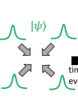
Figure 3: Generation of the pressure $\langle T^{\theta}{}_{\theta}\rangle_{*}$ and particles in the formation process of the dense configuration.

As the curvature increases, vacuum fluctuations of the other modes with various angular momenta are induced, which generate the pressure as a non-perturbative effect in the self-consistent solution $(g_{\mu\nu}^{*},|\psi\rangle_{*})$ (see also Appendix C). Because of this quantum pressure, the excited quanta are not concentrated at the center, but are spread and distributed throughout the interior. As a result, the curvatures are kept finite as (33), and the center is still (almost) flat. In fact, in the anisotropic TOV equation, we can see that this pressure is balanced by the strong self-gravity foot:pressure .

Thus, we reach the picture shown in Fig.4.

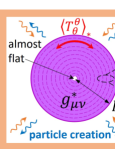
Figure 4: Left: The entropy-maximized configuration (31) in a heat bath of temperature $T_{0}$ (Hawking temperature). Right: The 1-bit quanta with $\lambda_{*}(r)\sim\sqrt{n}l_{p}$ distributed uniformly in the $\hat{r}$ direction.

The metric (31) represents a self-gravitating configuration consisting of the excited quanta, distributed uniformly in $\hat{r}$ direction, and the vacuum fluctuations. It is dense in the sense that it has the large pressure and curvatures. Here, we can check Y1 that the curvatures jump at the surface (located at (42)) in a mild manner to keep as much the interior uniformity as possible, consistent with Israel’s junction condition Poisson .

Let us now find a rough form of $A_{0}$ and consider what it means. First, we note from $a_{0}\approx a_{*}(R)=R-\frac{2\sigma}{R}$ that the surface exists at $r=R=a_{0}+\mathcal{O}\left(\frac{nl_{p}^{2}}{a_{0}}\right)$ (see (42) for the precise position). In order for the interior metric (31) to connect at $r=R$ to the exterior Schwarzschild metric with mass $\frac{a_{0}}{2G}$, the induced metric on $r=R$ must be continuous Poisson , which requires $-g_{tt}(R)=1-\frac{a_{0}}{R}=\frac{2\sigma}{R^{2}}e^{\frac{R^{2}}{2\sigma\eta}+A_{0}}$. Then, we can obtain

$$g_{tt}^{*}(r)=-\frac{2K\sigma}{r^{2}}e^{-\frac{R^{2}-r^{2}}{2\sigma\eta}},$$ (35)

where $K$ is a $\mathcal{O}(1)$ constant to be fixed. For $r=R-\Delta r$ ($\Delta r\ll R$), (35) becomes $-g_{tt}^{*}(r)\sim e^{-\frac{R\Delta r}{\sigma\eta}}$. This means that due to this large redshift, from the outside, a deep region of $\Delta r\gg\mathcal{O}\left(\frac{nl_{p}^{2}}{a_{0}}\right)$ is almost frozen in time (see KY5 for the details). As a result, although there is no horizon, the information carried by the excited quanta is kept inside for a long time KY2 .

Finally, we discuss how the dense configuration is formed. For example, we can obtain the metric (31) as a result of the semi-classical time evolution of adiabatic formation in a heat bath KY1 ; KY5 . Note here that generically, particle creation occurs in a time-dependent spacetime BD ; Barcelo . Indeed, in a time-dependent metric where radiations are coming together as in Fig.3, particles are created at Hawking temperature KMY ; KY4 . By slowly changing the temperature of the heat bath to match the Hawking temperature of the energy at each stage and considering the backreaction from the evaporation through (2), the dense configuration will be formed slowly.

We can see that this adiabatic formation is consistent with Bekenstein’s idea Bekenstein . At each stage where the mass is $\frac{a_{0}^{\prime}}{2G}$, a photon is emitted from the bath of $T_{H}^{\prime}=\frac{\hbar}{4\pi a_{0}^{\prime}}$ to the dense configuration with size $R^{\prime}=a_{0}^{\prime}+\mathcal{O}\left(\frac{nl_{p}^{2}}{a_{0}^{\prime}}\right)$. Since the wavelength $\sim a_{0}^{\prime}$ and the size $R^{\prime}$ are almost the same, the probability of the photon entering the dense region is roughly one-half, leading to 1 bit of information Bekenstein . On the other hand, the photon approaches to $r=R^{\prime}$ foot:r_i , and the blueshifted temperature becomes $T_{loc}(r=R^{\prime})=\frac{T_{H}^{\prime}}{\sqrt{1-\frac{a_{0}^{\prime}}{R^{\prime}}}}\sim\frac{m_{p}}{\sqrt{n}}\sim\epsilon_{max}$. Therefore, this photon corresponds to the 1-bit quantum, discussed in Sec.II, with $\epsilon_{max}$ and the 1 bit of information about its existence. Repeating this process, the uniform dense structure like Fig.4 appears, and the entropy follows the area law (24). In this sense, Bekenstein’s idea is realized, including the interior description at the level of (2).

Note also that when the configuration with mass $\frac{a_{0}}{2G}$ is moved out of the bath to the vacuum, it will evaporate in time $\Delta t\sim\frac{a_{0}^{3}}{nl_{p}^{2}}$ due to the particle creation KY1 ; KY5 .

V Maximum Entropy $S_{max}$

Following the derivation in Y1 , we show that the maximum entropy $S_{max}=S[g_{\mu\nu}^{*}]$ agrees with the Bekenstein-Hawking formula. We then identify the position of the surface, $R$, from a thermodynamical argument.

V.1 Bekenstein-Hawking formula

We first find the local temperature $T_{loc}^{*}(r)$. We note that the excited quanta composing the static configuration are in radially accelerated motion against gravity to stay there, and the required acceleration is $\alpha_{*}(r)=\frac{1}{\sqrt{2\eta^{2}\sigma}}+\mathcal{O}(r^{-1})$. Here, the proper acceleration $\alpha(r)\equiv|g_{\mu\nu}\alpha^{\mu}\alpha^{\nu}|^{\frac{1}{2}}=\frac{\partial_{r}\log\sqrt{-g_{tt}(r)}}{\sqrt{g_{rr}(r)}}$, $\alpha^{\mu}\equiv u^{\nu}\nabla_{\nu}u^{\mu}$, and $u^{\mu}\partial_{\mu}=(-g_{tt}(r))^{-\frac{1}{2}}\partial_{t}$. Then, we have $\alpha_{*}(r)\sim\mathcal{R}_{*}(r)^{1/2}\sim 1/\lambda_{*}(r)$, and we can apply the Unruh effect locally to the interior metric (31), albeit barely Jacobson ; Pad :

$$T_{loc}^{*}(r)=\frac{\hbar\alpha_{*}(r)}{2\pi}=\frac{\hbar}{2\pi\sqrt{2\sigma\eta^{2}}}+\mathcal{O}(r^{-1}),$$ (36)

which is $\sim\epsilon_{max}$ consistent with (6). Thus, the excited quanta behave, typically, like a local thermal state in the radial direction at the temperature (36). This result is kinematical and can be applied to any type of local degrees of freedom due to the universality of the Unruh effect. On the other hand, we have seen in the last part of Sec.IV.3 that (36) can be obtained dynamically through the particle creation during the formation process (see Y1 for an explicit proof). Therefore, the kinematical and dynamical results coincide, and (36) is robust.

At first glance, the fact that $T_{loc}^{*}(r)$ is constant might appear to contradict Tolman’s law, while its naive application to (35) for $r\ll R$ would lead to $T_{loc}(r)=\frac{T_{H}}{\sqrt{-g_{tt}^{*}(r)}}\sim\frac{\hbar}{\sqrt{\sigma}}e^{\frac{R^{2}}{4\sigma\eta}}$, violating the semi-classical condition (16). In general, Tolman’s law holds only if, in a stationary spacetime, thermal radiation (more generally, energy flow) can propagate between objects that are stationary with respect to each other within the considered time, including (if any) the effects of interaction with other modes and scattering by potentials Tolman ; Landau_SM . On the other hand, using the metric (31) with (35), the radial null geodesic equation is given by $\frac{dr(t)}{dt}=\pm\sqrt{K}\frac{2\sigma}{r^{2}}e^{-\frac{R^{2}-r^{2}}{4\sigma\eta}}$, which means that in the absence of interaction, it takes time $\Delta t\sim e^{a_{0}^{2}/l_{p}^{2}}$ for thermal radiation to travel a distance $\Delta r=\mathcal{O}(a_{0})$ inside the configuration.

Therefore, we can understand (36) as follows. Each part of the interior remains, due to the large redshift, at the temperature $T_{loc}(r)\sim\epsilon_{max}$ at the time of formation (see the end of Sec.IV.3), and only during $\Delta t<\mathcal{O}(e^{a_{0}^{2}/l_{p}^{2}})$ can the dense configuration exist consistent with Tolman’s law. In this sense, the interior is not in global equilibrium but in radially local one foot:T_loc2 , which is consistent with the self-consistent state $|\psi\rangle_{*}$ above (32). This may be some kind of global equilibrium, which will be discussed in Sec.VII. Note here that the time scale $\sim e^{a_{0}^{2}/l_{p}^{2}}$ is much longer than the evaporation time scale $\sim\frac{a_{0}^{3}}{l_{p}^{2}}$, and we can discuss the configuration physically.

Now, in this local equilibrium, the 1D Gibbs relation

$$T_{loc}s=\rho_{1d}+p_{1d}$$ (37)

holds for $\rho_{1d}=4\pi r^{2}\langle-T^{\hat{t}}{}_{\hat{t}}\rangle$ and $p_{1d}=4\pi r^{2}\langle T^{\hat{r}}{}_{\hat{r}}\rangle$, since the configuration is uniform in the proper radial length $\hat{r}$ Groot . Also, from (IV.3), $p_{1d}^{*}=\frac{2-\eta}{\eta}\rho_{1d}^{*}$ plays the role of the equation of state because $\langle T^{\theta}{}_{\theta}\rangle_{*}$ comes from the vacuum and thus has no thermodynamic contribution. These together with (36) and (IV.3) provide

$$s_{*}(r)=\frac{\rho_{1d}^{*}+p_{1d}^{*}}{T_{loc}^{*}}=\frac{1}{T_{loc}^{*}}\frac{2}{\eta}\rho_{1d}^{*}=\frac{2\pi\sqrt{2\sigma}}{l_{p}^{2}},$$ (38)

which is $\sim\frac{\sqrt{n}}{l_{p}}$ and consistent with one below (26). This and (31) lead to the Bekenstein-Hawking formula Bekenstein ; Hawking :

$$S_{max}=\int^{R}_{0}dr\sqrt{g^{*}_{rr}}s_{*}=\int^{R}_{0}dr\sqrt{\frac{r^{2}}{2\sigma}}\frac{2\pi\sqrt{2\sigma}}{l_{p}^{2}}=\frac{{\cal A}}{4l_{p}^{2}},$$ (39)

although there is no horizon, where ${\cal A}\equiv 4\pi R^{2}=4\pi a_{0}^{2}+\mathcal{O}(1)$. This gives the precise version of (24), and thus (20) and (39) mean (3).

Note that while the entropy density (38) depends on the species of fields and equation of state through $\sigma$ in (32), $\sigma$ cancels out in (39), leading to the universal coefficient. This is a result of the self-consistent treatment of the self-gravity and (36).

V.2 Surface

We determine the size $R$ from thermodynamics Y1 . Imagine that the configuration is in equilibrium with a heat bath of temperature $T_{0}$ during $\Delta t<\mathcal{O}(e^{a_{0}^{2}/l_{p}^{2}})$ (see Fig.4). From thermodynamic relation $T_{0}dS=dM_{0}$ ($M_{0}=\frac{a_{0}}{2G}$) and (39), the equilibrium temperature is fixed as the Hawking temperature:

$$T_{0}=\frac{\hbar}{4\pi a_{0}}.$$ (40)

Now, radiation emitted from the bath at $r\gg a_{0}$ comes close to the surface at $r=R$, and according to Tolman’s law in the Schwarzschild metric, the blueshifted temperature is given by $\frac{T_{0}}{\sqrt{1-\frac{a_{0}}{R}}}$. Then, thermodynamics requires that the local temperature be continuous at $r=R$ Landau_SM :

$$T_{loc}^{*}(R)=\frac{T_{0}}{\sqrt{1-\frac{a_{0}}{R}}}.$$ (41)

Setting $R=a_{0}+\Delta$ ($\Delta\ll a_{0}$) and using (36) and (40), (41) becomes $\frac{\hbar}{2\pi\sqrt{2\sigma\eta^{2}}}=\frac{\hbar}{4\pi a_{0}}\frac{1}{\sqrt{\frac{\Delta}{R}}}\approx\frac{\hbar}{4\pi\sqrt{a_{0}\Delta}}$, leading to $\Delta=\frac{\sigma\eta^{2}}{2a_{0}}$. We thus obtain

$$R=a_{0}+\frac{\sigma\eta^{2}}{2a_{0}}.$$ (42)

Note that the proper length $\sqrt{g_{rr}^{*}(R)}\frac{\sigma\eta^{2}}{2a_{0}}\sim\sqrt{n}l_{p}~{}(\gg l_{p})$ is independent of $a_{0}$.

Thus, using (42) to determine $A_{0}$ in the same procedure to get (35), we obtain the complete form of $g_{\mu\nu}^{*}$:

$$ds^{2}=-\frac{\sigma\eta^{2}}{2r^{2}}e^{-\frac{R^{2}-r^{2}}{2\sigma\eta}}dt^{2}+\frac{r^{2}}{2\sigma}dr^{2}+r^{2}d\Omega^{2}.$$ (43)

VI Bousso bound

In this section, we use the results obtained so far to derive the Bousso bound. We then confirm that the entropy-maximized configuration saturates not only the Bousso bound but also the local sufficient conditions proposed in the literature.

VI.1 Verification of the Bousso bound

We show that the Bousso bound holds in our class of spacetime. We first check that the entropy evaluated on a $t$-constant spacelike hypersurface $\Sigma_{t}$ inside the surface at $r=R$, which we have considered so far, agrees with one evaluated on a spherical ingoing null hypersurface $\Sigma_{L}$ starting from the surface and converging at $r=0$, a light sheet (roughly, a non-expanding null surface) proposed in Bousso1 . Here, we suppose that all configurations satisfy (2) and are regular. Applying $\nabla_{\mu}s^{\mu}=0$ to a closed spacetime region $V$ enclosed with $\Sigma_{t}$ and $\Sigma_{L}$ ($\partial V=\Sigma_{L}-\Sigma_{t}$. See Fig.5)

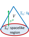
Figure 5: A spacetime region $V$ enclosed with $\Sigma_{t}$ and $\Sigma_{L}$.

and using Gauss’ theorem, we obtain

$$0=\int_{V}d{\mathcal{V}}\nabla_{\mu}s^{\mu}=\int_{\partial V}d\Sigma_{\mu}s^{\mu}\Rightarrow\int_{\Sigma_{t}}d\Sigma_{\mu}s^{\mu}=\int_{\Sigma_{L}}d\Sigma_{\mu}s^{\mu}.$$ (44)

Therefore, the entropy $S[g_{\mu\nu}]$, (15), agrees with the covariant entropy. Then, combining this and (3), we obtain the Bousso bound Bousso1 .

Thus, from this result and the discussion so far, we conclude that in the class of spherically-symmetric static spacetime, only (43) saturates the Bousso bound.

VI.2 Sufficient conditions for the Bousso bound

We study the relation of our discussion and the sufficient conditions proposed in FMW ; BFM for the Bousso bound and check the consistency.

First, we prepare ingredients to be used below. In a static spherical configuration with metric (4), the relation of entropy density $s$ and entropy current $s^{\mu}$ is as follows. For a $t$-constant hypersurface in (4), we have $d\Sigma_{\mu}=-u_{\mu}\sqrt{g_{rr}}r^{2}\sin\theta drd\theta d\phi$ with $u_{\mu}dx^{\mu}=-\sqrt{-g_{tt}}dt$ Poisson . Then, (1) gives $s=4\pi r^{2}(-u_{\mu}s^{\mu})$, i.e.,

$$s(r)=4\pi r^{2}\sqrt{-g_{tt}(r)}s^{t}(r),$$ (45)

and the entropy current is given by $s^{\mu}\partial_{\mu}=s^{t}\partial_{t}$.

We consider a spherical light sheet. A radially-ingoing null vector $k^{\mu}$ tangent to a geodesic generating it satisfies $0=g_{\mu\nu}k^{\mu}k^{\nu}=g_{tt}(k^{t})^{2}+g_{rr}(k^{r})^{2}$, leading to

$$\left(\frac{k^{t}}{k^{r}}\right)^{2}=\frac{g_{rr}}{-g_{tt}}.$$ (46)

Using this, we can calculate for a spherical static energy-momentum tensor $\langle T_{\mu\nu}(r)\rangle$

$$\langle T_{\mu\nu}\rangle k^{\mu}k^{\nu} =\langle T_{tt}\rangle(k^{t})^{2}+\langle T_{rr}\rangle(k^{r})^{2}$$

$$=g_{rr}(k^{r})^{2}\left(\left(\frac{k^{t}}{k^{r}}\right)^{2}\frac{-g_{tt}}{g_{rr}}\langle-T^{t}{}_{t}\rangle+\langle T^{r}{}_{r}\rangle\right)$$

$$=g_{rr}|k^{r}|^{2}\left(\langle-T^{t}{}_{t}\rangle+\langle T^{r}{}_{r}\rangle\right).$$ (47)

VI.2.1 Meaning of the upper bound (18)

The first sufficient condition, Eq.(1.9), suggested in FMW (or one in Pesci ) is given by

$$|-s^{\mu}k_{\mu}|\lesssim\frac{1}{\hbar}\Delta\zeta\langle T_{\mu\nu}\rangle k^{\mu}k^{\nu},$$ (48)

where $\Delta\zeta$ is the (finite) affine length of a geodesic along $k^{\mu}$ generating a light sheet in which quanta contributing to the entropy are included completely. (48) is a kind of light ray equivalent of Bekenstein’s bound (21), since $\Delta\zeta$ and $\langle T_{\mu\nu}\rangle k^{\mu}k^{\nu}$ correspond to $R$ and $M_{0}$, respectively.

We here show that the origin (18) of the upper bound (20) is a static spherical version of (48). First, we apply (45) to (18) and get

$$s^{t}\lesssim\frac{1}{\hbar}\sqrt{\frac{g_{rr}}{-g_{tt}}}(r-a(r))\langle-T^{t}{}_{t}\rangle.$$ (49)

We here have $|-s^{\mu}k_{\mu}|=|-s^{t}k_{t}|=s^{t}(-g_{tt})|k^{t}|$. Also, for excitations consistent with thermodynamics, $\langle-T^{t}{}_{t}\rangle\sim\langle T^{r}{}_{r}\rangle$ holds Landau_SM , and (VI.2) means $\langle T_{\mu\nu}\rangle k^{\mu}k^{\nu}\sim g_{rr}|k^{r}|^{2}\langle-T^{t}{}_{t}\rangle$. Using these, (49) leads to

$$|-s^{\mu}k_{\mu}| \lesssim\frac{1}{\hbar}\sqrt{\frac{-g_{tt}}{g_{rr}}}\frac{|k^{t}|}{|k^{r}|}\frac{r-a(r)}{|k^{r}|}\langle T_{\mu\nu}\rangle k^{\mu}k^{\nu}$$

$$=\frac{1}{\hbar}\frac{r-a(r)}{|k^{r}|}\langle T_{\mu\nu}\rangle k^{\mu}k^{\nu},$$ (50)

where (46) is applied. In terms of the affine parameter $\zeta$ of the geodesic, we have $k^{r}=\frac{dr(\zeta)}{d\zeta}$ and express $\frac{r-a(r)}{|k^{r}|}=\left|\frac{d\zeta}{dr}\right|(r-a(r))=\Delta\zeta$. Thus, (VI.2.1) provides (48) at each $r$ along the geodesic.

We discuss the meaning of this $\Delta\zeta$. In general, when considering a light sheet going to a horizon, the light sheet must not be continued to the interior, since the horizon entropy contains the contribution from objects that fell inside: Otherwise, it would be counted twice Bousso2 . In the geometry (4) without trapped surface, the “would-be horizon” for a point $r$ exists at $r=a(r)$. Therefore, our $\Delta\zeta$ represents the affine distance from a point to the “would-be end point”, and hence our $\Delta\zeta$ corresponds to that of Eq.(1.9) in FMW .

Thus, we conclude from the arguments in the previous sections that the spacetime $g_{\mu\nu}^{*}$ (43) is derived as a necessary condition for saturating (48), Eq.(1.9) in FMW .

VI.2.2 Exact saturation of a sufficient condition by $g_{\mu\nu}^{*}$

The sufficient condition, Eq.(3.5), proposed in BFM is

$$|k^{\mu}k^{\nu}\nabla_{\mu}s_{\nu}|\leq\frac{2\pi}{\hbar}\langle T_{\mu\nu}\rangle k^{\mu}k^{\nu},$$ (51)

which is motivated by an argument on the non-locality of entropy. We show that the entropy-maximized configuration $g_{\mu\nu}^{*}$, (43), saturates this exactly.

We first construct the spherically-symmetric static version of (51). From (45), we have $s_{\mu}dx^{\mu}=s_{t}dt$ with $s_{t}=-\frac{\sqrt{-g_{tt}}}{4\pi r^{2}}s$. We can calculate in (4)

$$k^{\mu}k^{\nu}\nabla_{\mu}s_{\nu}$$

$$=k^{t}k^{r}(\nabla_{t}s_{r}+\nabla_{r}s_{t})$$

$$=k^{t}k^{r}\sqrt{-g_{tt}}\left(\frac{s}{4\pi r^{2}}\partial_{r}\log\sqrt{-g_{tt}}-\partial_{r}\left(\frac{s}{4\pi r^{2}}\right)\right).$$ (52)

From this and (VI.2), (51) becomes

$$\langle-T^{t}{}_{t}\rangle+\langle T^{r}{}_{r}\rangle$$

$$\geq\frac{\hbar}{2\pi}\frac{\sqrt{-g_{tt}}}{g_{rr}}\frac{|k^{t}|}{|k^{r}|}\left|\frac{s}{4\pi r^{2}}\partial_{r}\log\sqrt{-g_{tt}}-\partial_{r}\left(\frac{s}{4\pi r^{2}}\right)\right|$$

$$=\frac{\hbar}{2\pi}\left|\frac{\partial_{r}\log\sqrt{-g_{tt}}}{\sqrt{g_{rr}}}\frac{s}{4\pi r^{2}}-\frac{1}{\sqrt{g_{rr}}}\partial_{r}\left(\frac{s}{4\pi r^{2}}\right)\right|$$ (53)

where we have applied (46). We then use the acceleration $\alpha=\frac{\partial_{r}\log\sqrt{-g_{tt}}}{\sqrt{g_{rr}}}$ to obtain

$$\left|\frac{\hbar\alpha}{2\pi}\frac{s}{4\pi r^{2}}-\frac{\hbar}{2\pi}\frac{1}{\sqrt{g_{rr}}}\partial_{r}\left(\frac{s}{4\pi r^{2}}\right)\right|\leq\langle-T^{t}{}_{t}\rangle+\langle T^{r}{}_{r}\rangle.$$ (54)

The metric (43) saturates this exactly at the leading order for $r\gg l_{p}$: The left hand side becomes $\frac{\hbar\alpha_{*}}{2\pi}\frac{s_{*}}{4\pi r^{2}}-\frac{\hbar}{2\pi}\frac{1}{\sqrt{g^{*}_{rr}}}\partial_{r}\left(\frac{s_{*}}{4\pi r^{2}}\right)\approx\frac{\hbar\alpha_{*}}{2\pi}\frac{s_{*}}{4\pi r^{2}}=\frac{1}{4\pi G\eta r^{2}}$ for $r\gg l_{p}$ (from (36) and (38)), while the right one becomes $\langle-T^{t}{}_{t}\rangle_{*}+\langle T^{r}{}_{r}\rangle_{*}=\frac{1}{4\pi G\eta r^{2}}$ (from (IV.3)).

Thus, the spacetime $g_{\mu\nu}^{*}$ (43) saturates the local condition (51), Eq.(3.5) in BFM . This is so non-trivial that there must be something behind it.

VII Conclusions and Discussions

In the class of spherically-symmetric static spacetimes with sufficiently excited states, we have evaluated entropy including the full self-gravity in the WKB approximation, and from the necessary condition that maximizes it, we have found uniquely the solution to the 4D semi-classical Einstein equation for a large $n$, leading to the Bousso bound. Such a dynamical and direct approach differs from the other ones. The solution is non-perturbative in $\hbar$, leading to the species bound, and it represents the radially uniform dense configuration with near-Planckian curvatures, not horizon or singularity. Its entropy saturates the Bousso bound and coincides with the Bekenstein-Hawking formula. It also saturates exactly the local sufficient condition for the Bousso bound. Therefore, this spacetime structure with strong gravity and large quantum effects should qualitatively exhibit, albeit at the semi-classical level, some non-perturbative behavior of quantum gravity, leading to the understanding of holographic principle. Let us discuss some future avenues in this direction.

First, we want to clarify the essence of the entropy-area law. The key question for this is, “How does the self-gravity $g_{\mu\nu}^{*}$ suppress the excitation of the local degrees of freedom?” From (38), the entropy per unit proper volume is given by $\frac{s_{*}(r)}{4\pi r^{2}}=\mathcal{O}\left(\frac{\sqrt{n}}{l_{p}r^{2}}\right)$, which is much smaller than the naive estimate, $\mathcal{O}\left(\frac{n}{l_{p}^{3}}\right)$ Bousso2 . This gap should be related to the self-consistent state $|\psi\rangle_{*}$ described above (32) (and (76)). Also, the radial uniformity (26), leading to (24), should be involved, and one could consider it as a realization of holography: the data at the boundary continues uniformly inside and determines the bulk (see also Appendix B). We will examine these points and answer the question.

Second, the energy scale of the dense configuration is $\sim\frac{m_{p}}{\sqrt{n}}$ (from (33) and (36)) and close to the Planck scale, and the configuration is described only at a resolution of about $\Delta\hat{r}\sim\sqrt{n}l_{p}$ and holds for any degree of freedom with that level of locality. Therefore, it should be interesting to search for such a “non-local” degree of freedom for an effective description of the configuration in quantum gravity. This could be along the direction above.

Third, we have utilized the WKB-like method for highly excited states to evaluate entropy $S[g_{\mu\nu}]$ incorporating self-gravity dynamically. This is considered complementary to methods that are more directly rooted in quantum theory, though not fully considering the self-consistent gravity Minic ; Casini ; BCFM ; Francesco ; f_con . Thus, a successful fusion of the two should allow us to refine the present entropy evaluation and treat other classes of spacetime (say, non-spherically symmetric or time-dependent ones) to explore more deeply the meaning of the Bousso bound.

Fourth, the only component of the Einstein equation that is explicitly used to reach the area law (24) is the Hamiltonian constraint (13). This reminds us the fact that the Hamiltonian constraint is applied to obtain Wald entropy Wald . Therefore, when considering the dynamics of gravity, the total entropy of matter and gravity may in general be a gravitational charge Y1 ; SY . For this aspect, it is also interesting to study the relationship between the maximum entropy (39) and the generalized entropy f_con involving both contributions from geometry and matter.

Finally, the relation between the entropy-maximized configuration and the second law of thermodynamics is interesting. The upper bound (20) is obtained from the geometric condition (17) and does not seem to be directly related to the second law. Also, the entropy-maximized configuration is not in a global equilibrium in the sense that Tolman’s law does not hold, although the configuration can be formed adiabatically KY1 ; KY5 . These should be closely related each other, leading to a new kind of global equilibrium. For this, we can make a conjecture.

When the dense configuration is formed in a heat bath adiabatically, (17) is saturated as a result of the time evolution KY1 ; foot:r_i . In thermodynamics, such an adiabatic process should yield the most typical configuration Landau_SM . Therefore, the dense configuration should be a global equilibrium state with the maximum entropy according to the second law.

Here, the effect of interactions should be involved significantly. First, thermal equilibrium is generally achieved through interactions Landau_SM . Second, the typical energy scale inside is close to the Planck scale, and some quantum-gravity effect may appear approximately where various degrees of freedom interact like, say, string. Indeed, we can model such interactions and show that ingoing radiation from the bath and outgoing radiation created inside interact around the surface in a time scale $\Delta t\sim a_{0}\log\frac{a_{0}}{nl_{p}}$, which makes the system stationary KY2 . We can then expect that due to many such interactions inside, energy should be transferred as conductive heat rather than radiative heat, and the propagation time scale should be longer than $\Delta t\sim\mathcal{O}(e^{a_{0}^{2}/l_{p}^{2}})$ (see Sec.V.1) so that the dense uniform configuration exists as a global equilibrium state, a strong-gravity “phase” of semi-classical quanta characterized by the entropy-area law. We will study this possibility in future.

Y.Y. thanks C.Barcelo, F.Becattini, R.Casadio, C.Y.Chen, C.Goeller, T.Harada, C.Kelly, E.Livine, A.Pesci, and Y.Sakatani for inspiring discussions and valuable comments. Y.Y. is partially supported by Japan Society of Promotion of Science (Grants No.21K13929) and by RIKEN iTHEMS Program.

Appendix A Self-gravitating thermal radiation

To demonstrate the self-gravity dependence of entropy explicitly in an example, we provide a review for self-gravitating thermal radiation and derive the entropy. We also check its consistency to $S[g_{\mu\nu}]$ and the upper bound.

A.1 Metric

We consider a spherically-symmetric static configuration of self-gravitating ultra-relativistic fluid with size $R$, mass $M_{0}=\frac{a_{0}}{2G}$, and equation of state $\rho=3p$, where $\rho(r)\equiv\langle-T^{t}{}_{t}(r)\rangle$ and $p(r)\equiv\langle T^{r}{}_{r}(r)\rangle=\langle T^{\theta}{}_{\theta}(r)\rangle$. For simplicity, we here neglect a small contribution from Weyl anomaly from the curvatures BD and interactions fluidbook . We construct its interior metric, for (4), in a heuristic manner. (See Weinberg for a more formal derivation.)

First, the equation of state $\rho=3p$, equivalent to $\langle T^{\mu}{}_{\mu}\rangle=0$, means that there is no special length scale in the system. Therefore, the order of the magnitude of the curvature at $r$ should be $\mathcal{R}(r)\sim\frac{1}{r^{2}}$. Also, $\rho=3p$ indicates $\rho\sim p$, and both $\rho$ and $p$ contribute to the curvature almost equally. Thus, from the Einstein equation (2), we have $\rho(r)\sim\frac{1}{Gr^{2}}$, which can be expressed as $\rho(r)=\frac{1-C}{8\pi Gr^{2}}$ with a $\mathcal{O}(1)$ constant $C$. Applying (14) to this, we have

$$\frac{a(r)}{2G}=\frac{1-C}{2G}r.$$ (55)

This must be positive due to radiation excitation and must be smaller than $\frac{4r}{9G}$ from Buchdahl’s limit Buchdahl ; Weinberg , and thus $C$ must satisfy $\frac{1}{9}<C<1$. Then, the metric (4) becomes

$$ds^{2}=-Ce^{A(r)}dt^{2}+\frac{1}{C}dr^{2}+r^{2}d\Omega^{2}.$$ (56)

Next, $A(r)$ is determined from the ultra-relativistic fluid condition: $\langle-T^{t}{}_{t}\rangle=3\langle T^{r}{}_{r}\rangle$ and $\langle T^{r}{}_{r}\rangle=\langle T^{\theta}{}_{\theta}\rangle$. (56) gives

$$-G^{t}{}_{t} =\frac{1-C}{r^{2}},$$ (57)

$$G^{r}{}_{r} =-\frac{1-C}{r^{2}}+\frac{CA^{\prime}(r)}{r},$$ (58)

$$G^{\theta}{}_{\theta} =\frac{C}{2r}A^{\prime}(r)+\frac{1}{4}CA^{\prime}(r)^{2}+\frac{1}{2}CA^{\prime\prime}(r).$$ (59)

Using these and (2), $\langle-T^{t}{}_{t}(r)\rangle=3\langle T^{r}{}_{r}(r)\rangle$ leads to $A(r)=A_{0}+\frac{4(1-C)}{3C}\log r$ ($A_{0}$: constant). Applying this $A(r)$, (58) and (59) to $\langle T^{r}{}_{r}(r)\rangle=\langle T^{\theta}{}_{\theta}(r)\rangle$ through (2), we have $(1-C)(-4+7C)=0$, giving $C=\frac{4}{7}$, which is consistent with Buchdahl’s limit. Then, we get $A(r)=A_{0}+\log r$, and (56) becomes

$$ds^{2}=-\frac{4}{7}e^{A_{0}}rdt^{2}+\frac{7}{4}dr^{2}+r^{2}d\Omega^{2},$$ (60)

and the energy density is given by

$$\rho(r)=\frac{3}{56\pi Gr^{2}}.$$ (61)

Here, the size $R$ is determined by applying (55) with $C=\frac{4}{7}$ and $a(R)=a_{0}$:

$$R=\frac{7}{3}a_{0}.$$ (62)

Finally, we connect (60) to the Schwarzschild metric with mass $\frac{a_{0}}{2G}$. This requires the continuity of $-g_{tt}(r)$ at $r=R$ Poisson : $-g_{tt}(R)=\frac{4}{7}e^{A_{0}}R=1-\frac{a_{0}}{R}$, leading through (62) to $e^{A_{0}}=\frac{1}{R}$. Thus, we reach the final form:

$$ds^{2}=-\frac{4}{7}\frac{r}{R}dt^{2}+\frac{7}{4}dr^{2}+r^{2}d\Omega^{2}~{}~{}~{}{\rm for}~{}~{}r\leq R.$$ (63)

Note that the curvatures are small for $r\gg l_{p}$: $R_{\mu\nu\alpha\beta}R^{\mu\nu\alpha\beta}\sim\frac{1}{r^{4}}$. Therefore, the contribution from 4D Weyl anomaly BD is indeed small for $r\gg l_{p}$, where our approximation is valid.

A.2 Entropy

Now, let us evaluate the entropy. First, the equation of state $\rho=3p$ and thermodynamics lead to the Stefan-Boltzmann law:

$$\rho(r)=\frac{kn_{f}}{4\hbar^{3}}T_{loc}(r)^{4},$$ (64)

where $k$ is a $\mathcal{O}(1)$ numerical constant, and $n_{f}$ is the number of the degrees of freedom of radiation Landau_SM . This and (61) determine the local temperature at $r$:

$$T_{loc}(r)\sim\frac{n_{f}^{-\frac{1}{4}}\hbar}{\sqrt{l_{p}r}}.$$ (65)

Note that (65) agrees with one obtained by applying Tolman’s law Landau_SM to the metric (63), $\frac{T_{0}}{\sqrt{-g_{tt}(r)}}\sim r^{-\frac{1}{2}}$, and thus the metric (63) is consistent with both thermodynamics and general relativity.

Using $\rho=3p$, the Gibbs relation $\rho+p=T_{loc}\tilde{s}$ Groot , (64) and (65), we obtain the entropy per unit proper volume, $\tilde{s}(r)\equiv\frac{s(r)}{4\pi r^{2}}$, as

$$\tilde{s}(r)=\frac{kn_{f}}{3\hbar^{3}}T_{loc}(r)^{3}\sim\frac{n_{f}^{\frac{1}{4}}}{(l_{p}r)^{\frac{3}{2}}}.$$ (66)

Thus, applying (66) and (63) to (1), we get Sorkin

$$S=4\pi\int^{R}_{0}dr\sqrt{g_{rr}(r)}r^{2}\tilde{s}(r)\sim\int^{R}_{0}dr\frac{n_{f}^{\frac{1}{4}}}{l_{p}^{\frac{3}{2}}}r^{\frac{1}{2}}\sim n_{f}^{\frac{1}{4}}\left(\frac{R}{l_{p}}\right)^{\frac{3}{2}},$$ (67)

which is different from the usual volume law $\sim R^{3}$. This is a consequence of the self-gravity dependence of entropy. More precisely, however, the self-consistency with (2) needs to be checked as in Appendix C. That is, we must consider a theory in the metric (63), evaluate $\langle\psi|T_{\mu\nu}|\psi\rangle$ in a state $|\psi\rangle$ corresponding to the local Gibbs state Zubarev ; Francesco at the local temperature (65), solve (2), and show that (67) holds. We leave this task for another time.

A.3 Consistency check

We use this example to examine the consistency of our argument on $S[g_{\mu\nu}]$ and the upper bound.

First, the consistency of (11) to thermodynamics is checked by (12), which is obtained as the ratio between (64) and (66).

Second, we check the WKB/semi-classical conditions. We can use $\lambda(r)\sim\frac{\hbar}{\epsilon(r)}$, (6) and (65) to get $\lambda(r)\sim n_{f}^{\frac{1}{4}}\sqrt{l_{p}r}$, which is shorter than $\mathcal{R}(r)^{-\frac{1}{2}}\sim r$ (from (61)) for $r\gg l_{p}$, and the WKB condition (5) holds. We then have from this $\lambda(r)$, (7) and (61)

$$N(r)\sim n_{f}^{\frac{1}{2}}\frac{r}{l_{p}}.$$ (68)

The semi-classical condition (8) is satisfied for $r\gg l_{p}$.

Third, we study the relation to the second law. Locally $\frac{\partial\tilde{s}(r)}{\partial T_{loc}(r)}>0$ holds from (66), while for the whole part, we have $\frac{\partial S}{\partial T_{0}}<0$ indicating that the total heat capacity is negative Landau_SM , where we use (67) and $T_{0}=T_{loc}(R)\propto R^{-1/2}$ (from (65)). Thus, due to the long-range nature of gravity, the thermodynamic behavior is different depending on the region being considered.

Fourth, we check that thermal radiation does not saturate the sufficient conditions for the Bousso bound. We first study (18). The right hand side is evaluated as $\frac{1}{\hbar}\sqrt{g_{rr}(r)}(r-a(r))4\pi r^{2}\langle-T^{t}{}_{t}(r)\rangle\sim\frac{r}{l_{p}^{2}}$ from (61) and (63), while the left hand side as $s=4\pi r^{2}\tilde{s}\sim n_{f}^{\frac{1}{4}}\frac{r^{\frac{1}{2}}}{l_{p}^{\frac{3}{2}}}$ from (66). Therefore, (18) is not saturated for $r\gg l_{p}$ and not so large $n_{f}$.

We next examine (54). The right hand side becomes $\rho+p=\frac{4}{3}\rho=\frac{1}{14\pi Gr^{2}}$ from (61). For the left hand side, we have $\alpha(r)=\frac{\partial_{r}\log\sqrt{-g_{tt}(r)}}{\sqrt{g_{rr}(r)}}\sim\frac{1}{r}$ from (63) and obtain from (66) $\left|\frac{\hbar\alpha}{2\pi}\frac{s}{4\pi r^{2}}-\frac{\hbar}{2\pi}\frac{1}{\sqrt{g_{rr}}}\partial_{r}\left(\frac{s}{4\pi r^{2}}\right)\right|\sim\frac{n_{f}^{\frac{1}{4}}}{Gr^{2}}\sqrt{\frac{l_{p}}{r}}$. Thus, (54) is not saturated again.

Appendix B Entropy maximum from uniformity

We give another derivation of (23): we derive it from the condition $N(r)={\rm const}.\equiv N_{0}=\mathcal{O}(1)\gg 1$, instead of setting $\epsilon=\epsilon_{max}$. This indicates that radial uniformity is a sufficient condition for entropy maximization. Also, this may be related to a realization of holography as described in Sec.VII. Note that the discussion in the main text doesn’t depend on this Appendix.

We first combine (22) and (25) to get

$$N_{0}l_{p}^{2}\sim r(r-a_{*}(r))\partial_{r}a_{*}(r).$$ (69)

Here, $N(r)={\rm const.}$ means through (25) that $\epsilon(r)>0$ and $\partial_{r}a_{*}(r)>0$. Hence, we can solve $a_{*}=a_{*}(r)$ for $r$ to have $r=r(a)$ (here we write $a=a_{*}$ for simplicity) and express (69) as

$$\frac{dr(a)}{da}=\frac{1}{\gamma}r(a)(r(a)-a),$$ (70)

where $\gamma={\rm const.}=\mathcal{O}(N_{0}l_{p}^{2})$.

The general solution to (70) is given by

$$r(a)=\frac{e^{-x^{2}}}{C-\sqrt{\frac{\pi}{2\gamma}}{\rm erf}(x)},$$ (71)

where $C$ is an integration constant, $x\equiv\frac{a}{\sqrt{2\gamma}}$ and ${\rm erf}(x)\equiv\frac{2}{\sqrt{\pi}}\int^{x}_{0}dye^{-y^{2}}$. We are now considering a configuration with $\frac{a_{0}}{2G}\gg m_{p}$, and we can focus on the asymptotic form of (71) for $a\gg l_{p}$, that is, $x\gg 1$:

$$r(a)\approx\frac{e^{-x^{2}}}{\sqrt{\frac{\pi}{2\gamma}}-C+e^{-x^{2}}\left[\frac{1}{\sqrt{2\gamma}x}-\frac{1}{2\sqrt{2\gamma}x^{3}}+\mathcal{O}(x^{-5})\right]}.$$ (72)

If $\sqrt{\frac{\pi}{2\gamma}}-C\neq 0$, we would have $r(a)\sim e^{-x^{2}}$ for $x\gg 1$, but it is not consistent with $r,a\gg l_{p}$. Therefore, we must have $C=\sqrt{\frac{\pi}{2\gamma}}$. Then, we obtain

$$r(a) \approx\sqrt{2\gamma}x+\sqrt{\frac{\gamma}{2}}\frac{1}{x}+\mathcal{O}(x^{-3})$$

$$=a+\frac{\gamma}{a}+\mathcal{O}(a^{-3}),$$ (73)

which means for $a\gg l_{p}$

$$a_{*}(r)\approx r-\frac{\gamma}{r}.$$ (74)

We now substitute (74) into (25) to get

$$\epsilon(r)\sim\frac{m_{p}}{\sqrt{N_{0}}}.$$ (75)

Comparing this to (16), we find $N_{0}\sim n$. Therefore, (74) means (23).

Appendix C A self-consistent solution $(g_{\mu\nu}^{*},|\psi\rangle_{*})$

As a demonstration of our self-consistent argument, we give a short review for the derivation of the self-consistent value of $\sigma$ in (32), where we can see how quantum effects play key roles. (See KY4 for details.)

We start with a review about how to solve the semi-classical Einstein equation (2) self-consistently. First, we consider the physical system and problem of interest and construct a candidate metric $g_{\mu\nu}$ for it, say, by making a model or a thought experiment. Next, using that metric as a background spacetime, we examine the behavior of the matter fields and identify a candidate state $|\psi\rangle$ for the system. Then, we regularize the energy-momentum tensor and renormalize it to remove divergences. Finally, we equate the obtained renormalized energy-momentum tensor $\langle\psi|T_{\mu\nu}|\psi\rangle$ with the Einstein tensor $G_{\mu\nu}$ calculated from the metric and solve (2). If it can be solved consistently, our $(g_{\mu\nu},|\psi\rangle)$ is the self-consistent solution. If not, we set up another candidate and repeat the process again. This is how to solve (2) in a self-consistent manner. Note that the self-consistent method can also obtain a non-perturbative solution in $\hbar$.

Let’s implement this program by setting (31) for $r\leq R$ and the Schwarzschild metric with $a_{0}$ for $R\leq r$ as the candidate metric.

(1) Candidate state. First, we can consider the adiabatic formation process in a heat bath of Hawking temperature $\sim\frac{\hbar}{a_{0}}$ (see a discussion in Sec.IV.3) and study each mode of scalar field, $\phi(x)=e^{-i\omega t}\varphi(r)Y_{lm}(\theta,\phi)$, in the WKB approximation, to find that there exist two types of modes inside. One is a bound mode with various angular momenta $l$, which is trapped inside the dense configuration and cannot be excited due to a constraint from the Bohr-Sommerfeld quantization condition. The other is a continuum mode of s-waves, which can go to and from the outside and can be excited with $\omega\sim\frac{1}{a_{0}}$ to express thermal radiation from the bath and the Hawking radiation produced inside. Therefore, we set a candidate state $|\psi\rangle_{*}$ such that

$$\langle\psi|T_{\mu\nu}|\psi\rangle_{*}\approx\langle 0|T_{\mu\nu}|0\rangle+T_{\mu\nu}^{(\psi)}.$$ (76)

The first term is the contribution from the vacuum fluctuation of all modes in the ground state $|0\rangle$ in (31), and the second one is that from the excitation of the continuum mode of s-waves. We here assume that the second contribution is so excited that it can be approximated as a classical one.

(2) Regularization. To regularize the energy-momentum operator, we use the dimensional regularization scheme. In a $d=4+\epsilon$ dimensional spacetime, the semi-classical Einstein equation coupled with $n_{s}$ free massless scalar fields can be expressed as a regularized operator equation BD :

$$G_{\mu\nu}=8\pi G\left[\mu^{-\epsilon}T_{\mu\nu}-2\left(\frac{\hbar n_{s}}{1152\pi^{2}\epsilon}+\alpha(\mu)\right)H_{\mu\nu}\right.$$

$$\left.-2\left(-\frac{\hbar n_{s}}{2880\pi^{2}\epsilon}+\beta(\mu)\right)K_{\mu\nu}-2\left(\frac{\hbar n_{s}}{2880\pi^{2}\epsilon}+\gamma(\mu)\right)J_{\mu\nu}\right].$$ (77)

Here, $\hbar\mu$ is a renormalization point, $T_{\mu\nu}$ is the regularized energy-momentum tensor operator, and the other tensors are proportional to the identity operator. The counter terms with $1/\epsilon$ is chosen as those required by the minimal subtraction scheme, and each tensor is defined as, respectively, $H_{\mu\nu}\equiv\frac{1}{\sqrt{-g}}\frac{\delta}{\delta g^{\mu\nu}}\int d^{d}x\sqrt{-g}R^{2}$, $K_{\mu\nu}\equiv\frac{1}{\sqrt{-g}}\frac{\delta}{\delta g^{\mu\nu}}\int d^{d}x\sqrt{-g}R_{\alpha\beta}R^{\alpha\beta}$, and $J_{\mu\nu}\equiv\frac{1}{\sqrt{-g}}\frac{\delta}{\delta g^{\mu\nu}}\int d^{n}x\sqrt{-g}R_{\alpha\beta\gamma\delta}R^{\alpha\beta\gamma\delta}$. We also have the renormalized coupling constants at energy scale $\hbar\mu$:

$$\alpha(\mu) =\alpha_{0}-\frac{\hbar n_{s}}{2304\pi^{2}}\log\left(\frac{\mu^{2}}{\mu_{0}^{2}}\right),~{}$$

$$\beta(\mu) =\beta_{0}+\frac{\hbar n_{s}}{5760\pi^{2}}\log\left(\frac{\mu^{2}}{\mu_{0}^{2}}\right),~{}$$

$$\gamma(\mu) =-\frac{\hbar n_{s}}{5760\pi^{2}}\log\left(\frac{\mu^{2}}{\mu_{0}^{2}}\right).$$ (78)

Here, $\alpha_{0}$ and $\beta_{0}$ fix a 4D theory at energy scale $\hbar\mu_{0}$ while we have chosen $\gamma_{0}=0$ because of the 4D Gauss-Bonnet theorem. Thus, we can obtain a more explicit form of the renormalized energy-momentum tensor in the right hand side of (2):

$$\langle\psi|T_{\mu\nu}|\psi\rangle=\lim_{\epsilon\to 0}\left[\mu^{-\epsilon}\langle\psi|T_{\mu\nu}|\psi\rangle_{reg}\right.$$

$$-\frac{\hbar n_{s}}{1440\pi^{2}\epsilon}\left(\frac{5}{2}H_{\mu\nu}-K_{\mu\nu}+J_{\mu\nu}\right)$$

$$\left.-2(\alpha(\mu)H_{\mu\nu}+\beta(\mu)K_{\mu\nu}+\gamma(\mu)J_{\mu\nu})\right].$$ (79)

(3) Matter fields. We now focus on $\langle 0|T_{\mu\nu}|0\rangle$ in (76), which will lead to the self-consistent value of $\sigma$. To evaluate $\langle 0|T_{\mu\nu}|0\rangle_{reg}$, we solve the matter field equation $\Box\phi=0$ in the $(4+\epsilon)$-dimensional spacetime manifold $\mathcal{M}\times\mathbb{R}^{\epsilon}$, where $\mathcal{M}$ is our 4D physical spacetime (31) and $\mathbb{R}^{\epsilon}$ is $\epsilon$-dimensional flat spacetime KN :

$$ds^{2}=-\frac{2\sigma}{r^{2}}e^{\frac{r^{2}}{2\sigma\eta}}dt^{2}+\frac{r^{2}}{2\sigma}dr^{2}+r^{2}d\Omega^{2}+\sum_{a=1}^{\epsilon}(dy^{a})^{2}.$$ (80)

Using the fact that (31) is locally $AdS_{2}\times S^{2}$ (with AdS radius $L\equiv\sqrt{2\eta^{2}\sigma}$ and $S^{2}$ radius $r$), we can employ a $1/r$ expansion technique (for $r\gg L$) to solve $\Box\phi=0$ around $r=r_{0}(<R)$ perturbatively. Then, the 0-th order solution for the bound modes is given by

$$\phi(x)=\sum_{i}(a_{i}u_{i}^{(0)}(x)+a_{i}^{\dagger}u_{i}^{(0)\ast}(x)),$$ (81)

where $a_{i}|0\rangle=0$, $\sum_{i}=\sum_{n,l,m}\int d^{\epsilon}k$, and

$$u_{i}^{(0)}(t,r,\theta,\phi,y^{a})=$$

$$\sqrt{\frac{\hbar\eta}{2r_{0}}}\sqrt{\frac{\partial\omega_{nl}}{\partial n}}e^{-i\omega_{nl}t}e^{-\frac{r^{2}}{8\sigma\eta}}J_{j}(X)Y_{lm}(\theta,\phi)\frac{e^{ik\cdot y}}{(2\pi)^{\epsilon/2}}.$$ (82)

Here, $n$ represents the quantum number satisfying the Bohr-Sommerfeld quantization condition, the factors in front of $e^{-i\omega_{nl}t}$ is the normalization consistent with the condition and commutation relation, and $J_{j}(X)$ is the Bessel function, where $j\equiv\sqrt{L^{2}(l(l+1)/r_{0}^{2}+k^{2})+\frac{1}{4}}$ and $X\equiv Le^{\frac{r_{0}(r_{0}-r)}{2\sigma\eta}}\omega/\sqrt{-g_{tt}(r_{0})}$.

(4) Renormalization. After a long calculation using (81), we can obtain the leading term of $\langle 0|T_{\mu\nu}|0\rangle_{reg}$:

$$\mu^{-\epsilon}\langle 0|T^{\mu}{}_{\nu}|0\rangle_{reg}^{(0)}= \left(\begin{array}[]{cccc}1&&&\\ &1&&\\ &&-1&\\ &&&-1\end{array}\right)\mu^{-\epsilon}\langle 0|T^{t}{}_{t}|0\rangle_{reg}^{(0)}$$ (87)

$$+\left(\begin{array}[]{cccc}0&&&\\ &0&&\\ &&1&\\ &&&1\end{array}\right)\frac{\hbar n_{s}}{1920\pi^{2}\eta^{4}\sigma^{2}},$$ (92)

where the components are in the order of $(t,r,\theta,\phi)$ and

$$\mu^{-\epsilon}\langle 0|T^{t}{}_{t}|0\rangle_{reg}^{(0)}$$

$$=\frac{\hbar n_{s}}{960\pi^{2}\eta^{4}\sigma^{2}}\left[\frac{1}{\epsilon}+\frac{1}{2}\left(\gamma+\log\frac{1}{32\pi\eta^{2}\sigma\mu^{2}}\right)+c\right].$$ (93)

Here, $\gamma$ is Euler’s constant and $c$ is the non-trivial finite value for $|0\rangle$: $c=0.055868$. This can be renormalized by the counter terms in (C), giving

$$\langle 0|T^{\mu}{}_{\nu}|0\rangle^{(0)}= \left(\begin{array}[]{cccc}1&&&\\ &1&&\\ &&-1&\\ &&&-1\end{array}\right)\langle 0|T^{t}{}_{t}|0\rangle^{(0)}$$ (98)

$$+\left(\begin{array}[]{cccc}0&&&\\ &0&&\\ &&1&\\ &&&1\end{array}\right)\frac{\hbar n_{s}}{1920\pi^{2}\eta^{4}\sigma^{2}},$$ (103)

where

$$\langle 0|T^{t}{}_{t}|0\rangle^{(0)}$$

$$=\frac{\hbar n_{s}}{1920\pi^{2}\eta^{4}\sigma^{2}}\left[2c+\gamma+\log\frac{1}{32\pi\eta^{2}\sigma\mu^{2}_{0}}-\frac{960\pi^{2}}{\hbar n_{s}}(2\alpha_{0}+\beta_{0})\right].$$ (104)

is $\mathcal{O}(1)$. We note here that the trace part

$$\langle 0|T^{\mu}{}_{\mu}|0\rangle^{(0)}=\frac{\hbar n_{s}}{960\pi^{2}\eta^{4}\sigma^{2}}$$ (105)

is independent of $(\alpha_{0},\beta_{0})$.

(5) Self-consistent solution. Finally, we use (33), (76) and (105) and solve the trace part of (2) at the leading order:

$$(G^{\mu}{}_{\mu})^{(0)} =8\pi G\langle\psi|T^{\mu}{}_{\mu}|\psi\rangle^{(0)}$$

$$\Rightarrow\frac{1}{\sigma\eta^{2}} =8\pi G\frac{\hbar n_{s}}{960\pi^{2}\eta^{4}\sigma^{2}}$$

$$\Rightarrow\sigma =\frac{n_{s}l_{p}^{2}}{120\pi\eta^{2}},$$ (106)

which gives the self-consistent value of $\sigma$ in (32). Here, we have dropped the contribution from $T^{(\psi)\mu}{}_{\mu}$ because the mode integrations over $\omega$ and $l$ lead to $\mathcal{O}(1)$ terms in (98), and $T^{(\psi)\mu}{}_{\mu}$, including only s-waves, cannot produce a $\mathcal{O}(1)$ term.

Furthermore, we can consider $T_{\mu\nu}^{(\psi)}=\mathcal{O}(r^{-2})$ and calculate the 1st order contribution $\langle 0|T^{\mu}{}_{\mu}|0\rangle^{(1)}=\mathcal{O}(r^{-2})$ to find the self-consistent value of $\eta$ in a similar manner. Here, we need to choose a theory with $(\alpha_{0},\beta_{0})$ such that $\langle 0|T^{t}{}_{t}|0\rangle^{(0)}=0$ in (C) and $1\leq\eta<2$ in (32). Thus, we conclude that our candidate $(g_{\mu\nu}^{*},|\psi\rangle_{*})$ is the self-consistent solution for such a theory.

Here, we can see explicitly the origin of the large tangential pressure $\langle\psi|T^{\theta}{}_{\theta}|\psi\rangle^{*}$ in (IV.3). Under the condition that $\langle 0|T^{t}{}_{t}|0\rangle^{(0)}=0$, the second term in (98) gives

$$\langle 0|T^{\theta}{}_{\theta}|0\rangle^{(0)}=\frac{\hbar n_{s}}{1920\pi^{2}\eta^{4}\sigma^{2}}=\frac{15}{2Gn_{s}l_{p}^{2}},$$ (107)

where we have used (C). This is the half of (105), which agrees with the 4D Weyl anomaly BD ; Nicolai ; it already appears in the second term of (87); and it is a non-perturbative effect in that we cannot take the limit $\hbar\to 0$. Therefore, the pressure originates from the UV divergent structure ($\sim 1/\epsilon$) due to 4D quantum fluctuations induced by the curved spacetime (31) as in Fig.3.

References

- (1) G. ’t Hooft, Conf. Proc. C 930308 (1993), 284-296.
- (2) L. Susskind, J. Math. Phys. 36 (1995), 6377-6396.
- (3) L. Smolin, Nucl. Phys. B 601, 209-247 (2001).
- (4) R. Bousso, Rev. Mod. Phys. 74, 825-874 (2002).
- (5) J. D. Bekenstein, Phys. Rev. D 23, 287 (1981).
- (6) R. Bousso, JHEP 07, 004 (1999).
- (7) See (45) for the relation of and .
- (8) R. Tolman and P. Ehrenfest, Phys. Rev. 36, no.12, 1791-1798 (1930).
- (9) L. D. Landau and E. M. Lifshitz, Statistical Physics (Butterworth-Heinemann, Oxford, 1984).
- (10) R. D. Sorkin, R. M. Wald and Z. J. Zhang, Gen. Rel. Grav. 13, 1127-1146 (1981).
- (11) S. Goldstein, J. L. Lebowitz, R. Tumulka and N. Zanghi, Phys. Rev. Lett. 96, 050403 (2006).
- (12) S. Popescu, A. J. Short, and A. Winter, Nat. Phys. 2, 754 (2006).
- (13) A. Sugita, Nonlinear Phenom. Complex Sys. 10, 192 (2007).
- (14) P. Reimann, Phys. Rev. Lett. 99, 160404 (2007).
- (15) D.N.Zubarev, A.V.Prozorkevich, and S.A.Smolyanskii, Theoret. and Math. Phys. 40, 821 (1979).
- (16) F. Becattini and D. Rindori, Phys. Rev. D 99, no.12, 125011 (2019)
- (17) R. Bousso, E. E. Flanagan and D. Marolf, Phys. Rev. D 68, 064001 (2003).
- (18) R. Bousso, H. Casini, Z. Fisher and J. Maldacena, Phys. Rev. D 90, no.4, 044002 (2014).
- (19) G. Dvali, Fortsch. Phys. 58, 528-536 (2010).
- (20) G. Dvali and M. Redi, Phys. Rev. D 77, 045027 (2008).
- (21) H. Kawai, Y. Matsuo, and Y. Yokokura, Int. J. Mod. Phys. A 28, 1350050 (2013).
- (22) H. Kawai and Y. Yokokura, Int. J. Mod. Phys. A 30, 1550091 (2015).
- (23) H. Kawai and Y. Yokokura, Phys. Rev. D 93, no.4, 044011 (2016).
- (24) P. M. Ho, Class. Quant. Grav. 34, no. 8, 085006 (2017).
- (25) H. Kawai and Y. Yokokura, Universe 3, no.2, 51 (2017)
- (26) H. Kawai and Y. Yokokura, Universe 6, no.6, 77 (2020).
- (27) H. Kawai and Y. Yokokura, Phys. Rev. D 105, no.4, 045017 (2022).
- (28) Y. Yokokura, [arXiv:2207.14274 [hep-th]].
- (29) P. M. Ho, H. Kawai, H. Liao and Y. Yokokura, [arXiv:2307.08569 [hep-th]].
- (30) E. E. Flanagan, D. Marolf and R. M. Wald, Phys. Rev. D 62, 084035 (2000).
- (31) S. A. Hayward, Phys. Rev. D 53, 1938-1949 (1996).
- (32) This also means that we don’t only consider static configurations where Tolman’s law holds Francesco . See also Sec.V.1.
- (33) Edited by H. S. Leff and A. F. Rex, Maxwell’s demon 2: entropy, classical and quantum information, computing (Taylor and Francis, 2002)
- (34) N. D. Birrell and P. C. W. Davies, Quantum Fields in Curved space (Cambridge University Press, 1982).
- (35) J. D. Bekenstein, Phys. Rev. D 7, 2333 (1973); Phys. Rev. D 9, 3292 (1974).
- (36) P. Romatschke and U. Romatschke, Relativistic Fluid Dynamics In and Out of Equilibrium (Cambridge University Press, Cambridge, 2019).
- (37) L. D. Landau and E. M. Lifshitz, The Classical Theory of Fields (Butterworth-Heinemann, Oxford, 1980).
- (38) E. Poisson, A Relativistic Toolkit (Cambridge University Press, Cambridge, 2004).
- (39) T. Padmanabhan, Class. Quant. Grav. 4, L107-L113 (1987).
- (40) E. R. Caianiello and G. Landi, Lett. Nuovo Cim. 42, 70 (1985)
- (41) H. E. Brandt, Found. Phys. Lett. 2 (1989), 39.
- (42) M. Mars and J. M. M. Senovilla, Class. Quant. Grav. 20, L293-L300 (2003).
- (43) V. A. Antonov, Vest. Leningrad Univ. 7, 135 (1962).
- (44) D. Lynden-Bell and R. Wood, Mon. Not. Roy. Astron. Soc. 138, 495 (1968).
- (45) T. Padmanabhan, Phys. Rept. 188, 285 (1990).
- (46) In Ref.Sorkin , (III) and (21) were obtained for thermal radiation, while our derivation can be applied to more general configurations including non-fluid.
- (47) The proportionality to the area in (24) comes from . Such an energy density also appears in Roberto .
- (48) R. Casadio, Phys. Lett. B 843, 138055 (2023).
- (49) More precisely, we have . See KY4 ; KY5 for an explicit proof of .
-
(50)
The conservation law in the metric (4) gives
.
Applying (31) and (IV.3), only the second, third and last terms remain as the leading ones for :
This shows that the tangential pressure supports the configuration against the strong self-gravity. - (51) C. Barcelo, S. Liberati, S. Sonego and M. Visser, Phys. Rev. D 83, 041501 (2011).
- (52) In a simple model, we can see explicitly that as a result of the self-consistent time-evolution by (2), the photon will naturally approach while emitting particles at temperature KMY ; KY4 . Continuously repeating this, (23) will be obtained by time evolution.
- (53) T. Jacobson, Phys. Rev. Lett. 75, 1260-1263 (1995).
- (54) T. Padmanabhan, Rept. Prog. Phys. 73, 046901 (2010).
- (55) This non-global equilibrium makes the difference from Oppenheim .
- (56) J. Oppenheim, Phys. Rev. D 65, 024020 (2002); Phys. Rev. E 68, 016108 (2003).
- (57) S. R. de Groot and P. Mazur, Non-Equilibrium Thermodynamics (North-Holland, Amsterdam, 1962).
- (58) S. W. Hawking, Commun. Math. Phys. 43, 199 (1975) [Erratum-ibid. 46, 206 (1976)].
- (59) A. Pesci, Class. Quant. Grav. 24, 6219-6226 (2007); Class. Quant. Grav. 25, 125005 (2008).
- (60) D. Marolf, D. Minic and S. F. Ross, Phys. Rev. D 69, 064006 (2004).
- (61) H. Casini, Class. Quant. Grav. 25, 205021 (2008).
- (62) R. Bousso, Z. Fisher, S. Leichenauer and A. C. Wall, Phys. Rev. D 93, no.6, 064044 (2016).
- (63) R. M. Wald, Phys. Rev. D 48 (1993) no.8, R3427-R3431.
- (64) S. i. Sasa and Y. Yokokura, Phys. Rev. Lett. 116, no.14, 140601 (2016).
- (65) S. Weinberg, Gravitation and Cosmology (Wiley, 1972).
- (66) H. A. Buchdahl, Phys. Rev. 116, 1027 (1959).
- (67) H. Kawai and M. Ninomiya, Nucl. Phys. B 336, 115 (1990).
- (68) L. Casarin, H. Godazgar and H. Nicolai, Phys. Lett. B 787, 94-99 (2018).