Fast quantum gates based on Landau-Zener-Stückelberg-Majorana transitions

Abstract

Fast quantum gates are of paramount importance for enabling efficient and error-resilient quantum computations. In the present work we analyze Landau-Zener-Stückelberg-Majorana (LSZM) strong driving protocols, tailored to implement fast gates with particular emphasis on small gap qubits. We derive analytical equations to determine the specific set of driving parameters for the implementation of single qubit and two qubit gates employing single period sinusoidal pulses. Our approach circumvents the need to scan experimentally a wide range of parameters and instead it allows to focus in fine-tuning the device near the analytically predicted values. We analyze the dependence of relaxation and decoherence on the amplitude and frequency of the pulses, obtaining the optimal regime of driving parameters to mitigate the effects of the environment. Our results focus on the study of the single qubit $X_{\frac{\pi}{2}}$, $Y_{\frac{\pi}{2}}$ and identity gates. Also, we propose the $\sqrt{\rm{bSWAP}}$ as the simplest two-qubit gate attainable through a robust LZSM driving protocol.

I Introduction

One of the key ingredients in quantum computing is the ability to implement fast quantum gates, which are the essential building blocks to perform quantum algorithms. In recent years, significant progress has been made in the design of quantum gates using superconducting qubits, which become one of the most promising platforms due to their scalability, long coherence times, and potential for fast high-fidelity operationsKrantz et al. (2019); Kjaergaard et al. (2020); Kwon et al. (2021). The transmon qubit Koch et al. (2007) and the capacitively shunted flux qubit Yan et al. (2016) establish the basis for modern design of artificial atoms based on superconducting circuits. A more recent addition, the fluxonium, Manucharyan et al. (2009); Pop et al. (2014); Nguyen et al. (2019); Bao et al. (2022); Weiss et al. (2022); Somoroff et al. (2023), has a low transition frequency and a large anharmonicity, making it a promising candidate for quantum simulations and high-fidelity gate operations.

A variety of techniques for implementing fast quantum gates, including dynamical decoupling , composite pulses, and optimal control have been implemented so far Leek et al. (2007); Bylander et al. (2011); Yang et al. (2017); Wang et al. (2017); Zhu et al. (2021); Shen et al. (2021); Ficheux et al. (2021); Bastrakova et al. (2022); Chen et al. (2022). These techniques have led to significant improvements in gate fidelity. However, most of them rely on a resonant Rabi driving with frequency $\omega\approx\Delta=E_{1}-E_{0}$ (the qubit energy gap) and small amplitude, $A\ll\Delta$, whose duration is adapted to perform the target operation (throughout this article we take $\hbar=1$). As the gate time $t_{g}$ is inversely proportional to the generalized Rabi frequency, i.e. $t_{g}\propto\frac{1}{\Omega_{R}}\propto\frac{1}{A}$ Bloch and Siegert (1940), these schemes usually have limited gate speed involving time scales that are in conflict with those imposed by decoherence processes.

One approach to mitigating decoherence is to reduce the qubit coupling to the environment by using a low frequency, or small gaps qubit, as the heavy fluxonium. However, again in these cases, methods based on the Rabi resonant control would be unfeasible as $\Delta$ is small and in the rotating wave approximation (RWA) as $A\ll\Delta$ results $t_{g}\gg t_{\Delta}=\frac{2\pi}{\Delta}$.

To circumvent the mentioned limitations, alternatives beyond the resonant Rabi protocol have been recently proposed to experimentally implement fast gates with the decoherence time $t_{decoh}\gg t_{g}$Avinadav et al. (2014); Campbell et al. (2020); Zhang et al. (2021); Petrescu et al. (2023). One of these schemes is based on driving a composite qubit, formed from two capacitively coupled transmon qubits which has a small gap between two energy levelsCampbell et al. (2020). The qubit is controlled by a Landau-Zener-Stückelberg-Majorana (LZSM) driving protocol, which consist on driving the qubit with a strong amplitude and/or an off resonant harmonic signal Oliver et al. (2005); Sillanpää et al. (2006); Ferrón et al. (2012); Shevchenko et al. (2012); Ivakhnenko et al. (2023). LZSM protocols have been successfully implemented in interferometry of superconducting qubits Oliver and Valenzuela (2009); Berns et al. (2008), temporal oscillations Bylander et al. (2009) and used in the quantum simulation of universal conductance fluctuations and weak localization phenomena Gustavsson et al. (2013); Gramajo et al. (2020).

On the theoretical side, the study of the LZSM driving protocols requires the implementation of numerical methods, the most useful based on the Floquet formalism Shirley (1965); Son et al. (2009); Ferrón et al. (2012, 2016), as the RWA is valid in the weak driving and resonant cases, but breaks down in the strong driving regime where analytical and perturbative approaches fail. It is well known that the counter rotating terms lead to the shifts of resonances (Bloch-Siegert shift) and additional beat patterns in the time evolution Bloch and Siegert (1940); Shirley (1965) which are not captured in the RWA. In a quite recent paper Yan et al. (2015), the Bloch-Siegert shift was analytically obtained along the entire driving-strength regime, i.e. for $0<A/\omega<\infty$, by a simple analytical method based on an unitary transformation. The method uses a counter-rotating hybridized rotating wave approximation (CHRW) Lü and Zheng (2012); Yan et al. (2015); Chen et al. (2022) and enables to obtain an effective description of the qubit dynamics which reproduces the numerical results not only when the driving strength is moderately weak but also for strong driving strengths, far beyond the perturbation theory.

In the present work, we conduct an analysis of LZSM strong driving protocols suitable for implementing quantum gates in small gap qubits. By presenting precise analytical equations based on the CHRW approximation, we offer a method to determine the driving parameters (amplitude, frequency, initial and final idling times) required for both single qubit gates and the $\sqrt{bSWAP}$ gate. The approach eliminates the need for extensive experimental parameter scanning, allowing to concentrate on fine-tuning the device based on the analytically predicted parameters. We suggest the $\sqrt{bSWAP}$ gate as an ideal two-qubit gate achievable through a straightforward single one-period sinusoidal pulse using the strong driving LZSM protocol.

The paper is organized as follows: In Sec.II we introduce the counter-rotating hybridized rotating wave approximation (CHRW) to analyze the effective dynamics of the driven qubit Hamiltonian in terms of the operator $U(T)$, for a single period $T$ of a sinuosoidal drive. As a figure of merit for the accuracy of the CHRW we compute the error of this approximation, defined in terms of the Fidelity of the evolution with the operator $U(T)$ with respect to a target (exact numerically computed) unitary operator. In Secs. III and IV we analyze the implementation of single qubit $X_{\frac{\pi}{2}}$, $Y_{\frac{\pi}{2}}$ and two qubit $\sqrt{bSWAP}$ gates respectively, with special focus on the determination of the optimal driving parameters in order to engineering fast gates with strong non resonant LZSM protocols based on single period sinusoidal drives. The effect of relaxation and decoherence on the gate dynamics is analyzed in Sec.V. Finally the summary and conclusions are presented in Sec.VI.

II Effective dynamics for strongly driven qubits

We start by considering the standard two-level Hamiltonian modeling a driven qubit:

$$H(t)=-\frac{\Delta}{2}\hat{\sigma}_{z}-\frac{\epsilon(t)}{2}\hat{\sigma}_{x},$$ (1)

where $\hat{\sigma}_{z}$ and $\hat{\sigma}_{z}$ are the Pauli matrices and $\Delta$ is the qubit energy gap The Hamiltonian is written in the basis spanned by $|0\rangle$ and $|1\rangle$, which correspond to the ground and excited states of the qubit respectively. We consider a transverse driving protocol $\epsilon(t)=A\sin(\omega t)$, as used recently in small gap qubits like superconducting composite qubits Campbell et al. (2020) and heavy fluxonium qubits Weiss et al. (2022); Zhang et al. (2021).

For large gap qubits, like the transmon, the driving strength $A$ is typically small compared with the qubit gap $\Delta$, and qubit control and quantum gates are implemented in the Rabi-driving regime at resonant frequencies $\omega\approx\Delta$, that can be accurately described within the RWA. The recent development of highly coherent qubits with small gaps requires operation with non resonant fast drives $\omega>\Delta$ and large driving amplitudes, using control protocols based on LZSM transitions Oliver et al. (2005); Oliver and Valenzuela (2009); Ferrón et al. (2012); Shevchenko et al. (2012); Ivakhnenko et al. (2023). In this case, and in contrast with the Rabi-driving protocol, there are no simple expressions to predict the driving parameters needed for the implementation of quantum gates. Instead, calibration protocols scanning the pulse amplitude $A$ and frequency $\omega$ are usually performed in the experiments Campbell et al. (2020); Weiss et al. (2022); Zhang et al. (2021). For instance in Ref.Campbell et al. (2020), as a first step in the calibration protocol, the transition probability from the ground state to the excited state after a single period $T=2\pi/\omega$ of the sinusoidal drive, $P_{01}\equiv P_{|0\rangle\rightarrow|1\rangle}(T)$, is measured as a function of $A$ and $\omega$. From this scanned transition probability, values of $A$ and $\omega$ are chosen such that for these values $P_{01}$ corresponds to the implementation of a given quantum gate. In a second calibration step, idling times before and after the driving pulse are finely tuned-up in order to implement the desired quantum gate Campbell et al. (2020).

We have computed the time evolution with the $H(t)$ of Eq.(1) using a fourth order Trotter-Suzuki algorithm Hatano and Suzuki (2005a), to compare with the calibration protocol of Ref.Campbell et al. (2020). From the time evolution operator computed numerically, $U_{num}(t)$, we obtain $P_{01}=|\langle 1|U_{num}(T)|0\rangle|^{2}$ and plot it in Fig.1 as a function of $A$ and $\omega$, scanning the same range of values as in the experiment. The computed probabilities align closely with the experimental results shown in Fig.S3 of Ref.Campbell et al. (2020).

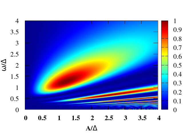
Figure 1: Transition probability $P_{01}=|\langle 1|U_{num}(T)|0\rangle|^{2}$ computed numerically using a fourth order Trotter-Suzuki algorithm. Intensity plot of $P_{01}$ as a function of the driving frequency $\omega$ and amplitude $A$, both normalized by the qubit gap $\Delta$. See text for details.

An analytical accurate estimation of the amplitude and frequency of the driving pulse could greatly simplify the calibration procedure. The difficulty is that large driving strengths require to go beyond the RWA and to account for counter-rotating effects. To obtain an effective description of the qubit dynamics an strategy is to use the CHRW approximation Lü and Zheng (2012); Yan et al. (2015); Chen et al. (2022), applied to this case. To this end, we start with the transformation $|\psi^{\prime}(t)\rangle=U_{x}|\psi(t)\rangle$, $H^{\prime}=U_{x}HU_{x}^{\dagger}+i(\partial_{t}U_{x})U_{x}^{\dagger}$, with $U_{x}=e^{-i\frac{\phi}{2}\hat{\sigma}_{x}}$. This gives Yan et al. (2015)

$$H^{\prime}=-\frac{(\epsilon-\dot{\phi})}{2}\hat{\sigma}_{x}-\frac{\Delta}{2}(\cos\phi\hat{\sigma}_{z}-\sin\phi\hat{\sigma_{y}}).$$ (2)

We take $\dot{\phi}=\xi\epsilon$, with $\xi$ a parameter to be determined later. Thus $\phi(t)=-\xi\frac{A}{\omega}\cos(\omega t)$ and $\exp{({i\phi})}=\exp{(-i\xi\frac{A}{\omega}\cos(\omega t))}$. Using the Jacobi-Anger expansion in terms of Bessel functions for:

$$e^{ix\cos a}=\sum_{k=-\infty}^{k=+\infty}i^{k}J_{k}(x)e^{ika}=J_{0}(x)+\sum_{k=1}^{\infty}2i^{k}J_{k}(x)\cos(ka),$$

we approximate in Eq.(2) (to lowest order in the Fourier expansion):

$$\cos\phi \approx J_{0}(\xi\frac{A}{\omega})$$

$$\sin\phi \approx -2J_{1}(\xi\frac{A}{\omega})\cos(\omega t),$$ (3)

and therefore

$$H^{\prime}=-\frac{\epsilon(1-\xi)}{2}\hat{\sigma}_{x}-\frac{\Delta}{2}\left[J_{0}(\xi\frac{A}{\omega})\hat{\sigma}_{z}+2J_{1}(\xi\frac{A}{\omega})\cos(\omega t)\hat{\sigma_{y}}\right],$$

which can be rewritten as:

$$H^{\prime}=-\frac{\widetilde{\Delta}}{2}\hat{\sigma}_{z}-\frac{1}{2}\left[A(1-\xi)\sin(\omega t)\hat{\sigma}_{x}+2\Delta J_{1}(a)\cos(\omega t)\hat{\sigma_{y}}\right],$$ (4)

with $\widetilde{\Delta}=\Delta J_{0}(a)$, and $a=\xi A/\omega$.

After expressing $\xi$ in terms of the self-consistent equation:

$$A(1-\xi)=2\Delta J_{1}(\xi\frac{A}{\omega})=\widetilde{A},$$ (5)

we can rewrite Eq.(4) as:

$$H^{\prime}=-\frac{\widetilde{\Delta}}{2}\hat{\sigma}_{z}-\frac{\widetilde{A}}{2}\left[\sin(\omega t)\hat{\sigma}_{x}+\cos(\omega t)\hat{\sigma_{y}}\right]$$ (6)

$$=-\frac{\widetilde{\Delta}}{2}\hat{\sigma}_{z}-\frac{\widetilde{A}}{2}\left[-ie^{i\omega t}\hat{\sigma}_{+}+ie^{-i\omega t}\hat{\sigma_{-}}\right].$$

which can be solved exactly. After transforming with the unitary operator $R=e^{-i\frac{\omega t}{2}\hat{\sigma}_{z}}$, we obtain:

$$H^{\prime\prime}=RH^{\prime}R^{\dagger}+i\frac{dR}{dt}R^{\dagger}$$

$$=-\frac{\widetilde{\delta}}{2}\hat{\sigma}_{z}-\frac{\widetilde{A}}{2}\hat{\sigma_{y}},$$ (7)

being $\widetilde{\delta}=\widetilde{\Delta}-\omega$.

Equation (7) can be easily diagonalized with the transformation $W=e^{-i\frac{\theta}{2}\hat{\sigma}_{x}}$, being $\tan\theta=\widetilde{A}/\widetilde{\delta}$, obtaining:

$$H_{d}=WH^{\prime\prime}W^{\dagger}=-\frac{\Omega_{R}}{2}\hat{\sigma}_{z},$$ (8)

with

$$\Omega_{R}=\sqrt{\widetilde{\delta}{{}^{2}}+\widetilde{A}{{}^{2}}}=\sqrt{[\Delta J_{0}(\xi\frac{A}{\omega})-\omega]^{2}+4\Delta^{2}J_{1}{{}^{2}}(\xi\frac{A}{\omega})},$$

the generalized Rabi frequency.

Taking into account the previous transformations, the evolution operator associated to Eq.(1), in the CHRW approximation, results :

$$U(t)=U_{x}^{\dagger}(t)R^{\dagger}(t)W^{\dagger}e^{i\frac{\Omega_{R}t}{2}\hat{\sigma}_{z}}WR(0)U_{x}(0).$$ (9)

In our case, for the implementation of fast quantum gates, we are interested in the evolution after one period of the driving, $T$, which is:

$$U(T)=-e^{i\frac{\theta-a}{2}\hat{\sigma}_{x}}e^{i\frac{\pi\Omega_{R}}{\omega}\hat{\sigma}_{z}}e^{-i\frac{\theta-a}{2}\hat{\sigma}_{x}}$$ (10)

$$=-\left(\begin{array}[]{cc}\cos\alpha+i\sin\alpha\cos{\tilde{\theta}}&\sin\alpha\sin{\tilde{\theta}}\\ -\sin\alpha\sin{\tilde{\theta}}&\cos\alpha-i\sin\alpha\cos{\tilde{\theta}}\end{array}\right),$$

with $\alpha=\frac{\pi\Omega_{R}}{\omega}$ and ${\tilde{\theta}}=\theta-a=\theta-\xi\frac{A}{\omega}$. The transition probability between the qubit states, $\left|0\right\rangle\rightarrow\left|1\right\rangle$, can then be obtained in this approximation as,

$$P_{01} = |\langle 1|U(T)|0\rangle|{{}^{2}}=\sin{{}^{2}}{\tilde{\theta}}\sin{{}^{2}}\alpha$$

$$= \frac{\left[\widetilde{A}\cos(\xi\frac{A}{\omega})-\widetilde{\delta}\sin(\xi\frac{A}{\omega})\right]{{}^{2}}}{\Omega_{R}^{2}}\sin{{}^{2}}\frac{\pi\Omega_{R}}{\omega}.$$

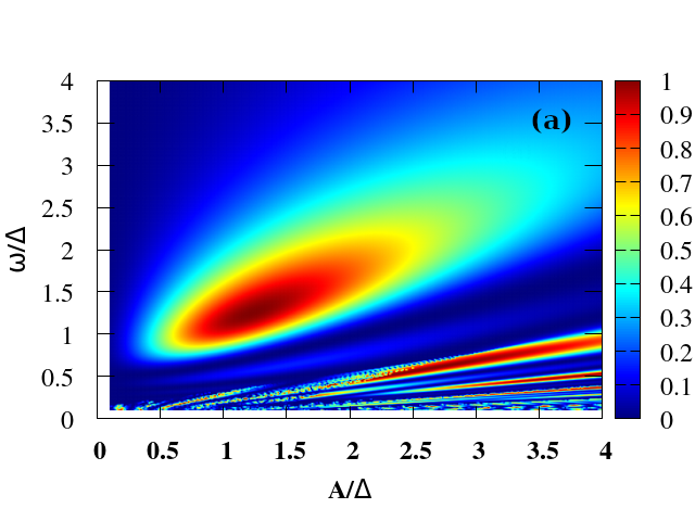
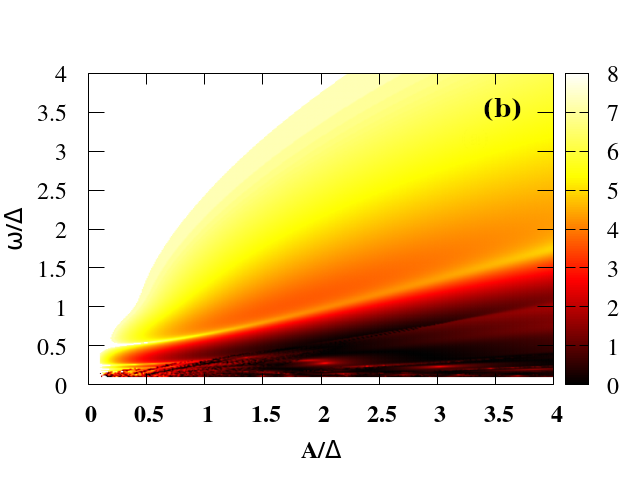
Figure 2: (a) Transition probability $P_{01}$ obtained from Eq.(II) as a function of driving frequency $\omega/\Delta$ and amplitude $A/\Delta$. (b) Plot of the error ${\cal E}$ of the CHRW approximation. The color scale of the intensity plot corresponds to $-\log_{10}|{\cal E}|$. Regions in white color correspond to ${\cal E}<10^{-8}$.

In Fig.2(a) we plot the transition probability computed from the analytical expression Eq.(II) as a function of the amplitude of the driving $A/\Delta$ and the frequency $\omega/\Delta$, (both normalized in terms of the qubit gap). The agreement with the numerical result of Fig.(1) is remarkable, despite some differences noticeable in the range of small $\omega/A$, due to numerical instabilities in the solution of Eq.(5) originated in the highly oscillatory behaviour of the Bessel function $J_{1}(x)$ for large values of its argument $x$.

In order to check the accuracy of the CHRW approximation we compare the approximated $U(T)$ of Eq.(10) with the the numerically exact $U_{num}(T)$. We quantify the error of the approximation as

$${\cal E}=1-{\cal F}=1-\frac{{\rm Tr}(U^{\dagger}U)+|{\rm Tr}(U_{tg}^{\dagger}U)|^{2}}{d(d+1)}\,.$$ (12)

where ${\cal F}$ is the standard expression for the fidelity of an evolution operator $U$ with respect to a target unitary operator $U_{tg}$ Pedersen et al. (2007). In the present case is $U_{tg}=U_{num}(T)$, with $d=2$ the dimension of the space, and ${\rm Tr}(U^{\dagger}U)=d$, as $U(T)$ is exactly unitary. In Fig.2(b) we plot the error ${\cal E}$. As expected Lü and Zheng (2012), the CHRW approximation is very accurate in the range $\omega\gtrsim A/2$ and $\omega\gtrsim\Delta$ (with ${\cal E}\ll 10^{-3}$), which is also the range of interest for the experiment of Ref.Campbell et al. (2020). Other methods of approximation as the Magnus expansion (used in Ref.Weiss et al. (2022)) and the RWA in a double rotating frame (used in Ref.Deng et al. (2015, 2016)) are much less accurate (see Appendix B for a comparison of the different approximations).

In the following sections we shall analyse different implementations of single and two qubit gates following this driving protocol.

III Implementation of single qubit gates

Here we analyze the conditions to implement fast single qubit gates with a strong driving protocol based on non resonant sinusoidal pulses (see Eq.(1)).

First, we note that $Z_{\alpha}=\exp(-i\alpha\hat{\sigma}_{z}/2)$ gates, can be realized by “idling” operations in the time evolution with the qubit set at $\epsilon=0$ for a time $t=\alpha/\Delta$, as implemented in Ref.Campbell et al. (2020). In addition to the continuous varying $Z_{\alpha}$ gate a complete set of single qubit gates can be realized, implementing for instance $X_{\pm\frac{\pi}{2}}=\exp(\mp i\pi\hat{\sigma}_{x}/4)$ and $Y_{\pm\frac{\pi}{2}}=\exp(\mp i\pi\hat{\sigma}_{y}/4)$ gates.

In the case of the $Y_{\frac{\pi}{2}}$ gate, we can write it in matrix form as:

$$Y_{\frac{\pi}{2}}=\frac{\sqrt{2}}{2}\left(\begin{array}[]{cc}1&-1\\ 1&1\end{array}\right).$$ (13)

A direct comparison of Eq.(13) with the CHRW expression for the operator $U(T)$, Eq.(10), gives the following condition to implement the $Y_{\frac{\pi}{2}}$ gate with the largest $\omega$:

$$\omega = \frac{4}{3}\Omega_{R},$$ (14)

$$\theta-\xi\frac{A}{\omega} = \frac{\pi}{2}$$

Numerical solution of these equations together with Eq.(5) give $\omega_{Y}\approx 2.07\Delta$ and $A_{Y}\approx 2.87\Delta$. The general conditions for the $Y_{\frac{\pi}{2}}$ gate are: $\omega=\Omega_{R}/(2k+3/4),\;{\tilde{\theta}}=(2l+1/2)\pi$ and $\omega=\Omega_{R}/(2k+5/4),\;{\tilde{\theta}}=(2l+3/2)\pi$, for $k,l$ integers. Solutions with $k\not=0,l\not=0$ give low $\omega$ and large $A$, beyond the parameter range for the CHRW approximation.

It is clear that the analytical estimate of the operational parameters for the gate implementation avoids the experimental cost of scanning parameters in a wide range. In the experiment, as described in the previous section, the fast gate is implemented applying the sinusoidal pulse for a single period $T=2\pi/\omega$, and the corresponding values of $A$ and $\omega$ are determined by performing different measurements scanning the amplitude and frequency. In a similar way, we can compute numerically the exact evolution operator $U_{num}(T)$ varying the parameters $\omega$ and $A$, for instance in the range $[0,4\Delta]$. To obtain the numerically exact conditions for the $Y_{\frac{\pi}{2}}$ gate, we show in Fig.3 the error function ${\cal E}$ from Eq.(12) with $U=U_{num}(T)$ compared with the target $U_{tg}=Y_{\frac{\pi}{2}}$. The point of minimum ${\cal E}$ (which is near the numerical precision for our calculation of $U_{num}(T)$, ${\cal E}\approx 10^{-7}$) corresponds to the operational point in $A,\omega$ for implementing the gate $Y_{\frac{\pi}{2}}$. This point agrees very accurately with the values $(A_{Y},\omega_{Y})$ computed previously from Eq.(14).

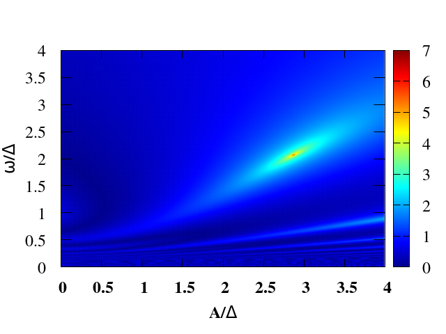
Figure 3: Location of the parameters for implementation of the $Y_{\frac{\pi}{2}}$ gate. Plot of the error function ${\cal E}$ that compares the numerically exact evolution operator $U_{num}$ with $Y_{\frac{\pi}{2}}$. The color scale of the intensity plot corresponds to $-\log_{10}|{\cal E}|$. The point where ${\cal E}<10^{-7}$ (practically zero within numerical precision) gives the operational parameters of the gate, frequency $\omega_{Y}$ and amplitude $A_{Y}$. It agrees with the analytical estimate of Eq.(14), $\omega_{Y}\approx 2.07\Delta$ and $A_{Y}\approx 2.87\Delta$.

In the case of the $X_{\frac{\pi}{2}}$ gate, its matrix representation is

$$X_{\frac{\pi}{2}}=\frac{\sqrt{2}}{2}\left(\begin{array}[]{cc}1&-i\\ -i&1\end{array}\right).$$ (15)

A comparison with the approximate $U(T)$ given in Eq.(10) shows that $X_{\frac{\pi}{2}}$ can not be realized directly, since $\sin\alpha\sin{\tilde{\theta}}\neq i$. However, one can add after the sinusoidal pulse an idle (Z gate) evolution McKay et al. (2017); Campbell et al. (2020) during a time $t_{f}=\frac{\pi}{\Delta}$, such that $e^{i\frac{\Delta}{2}\hat{\sigma}_{z}t_{f}}=i\hat{\sigma}_{z}$. Then, after the complete evolution given by $U(T+t_{f})=i\hat{\sigma}_{z}U(T)$, the main conditions to implement a $X_{\frac{\pi}{2}}$ gate result:

$$\omega = 2\Omega_{R},$$ (16)

$$\theta-\xi\frac{A}{\omega} = \frac{3\pi}{4}.$$

Numerical solution of these equations together with Eq.(5) give $\omega_{X}\approx 0.81\Delta$ and $A_{X}\approx 0.68\Delta$. The general conditions the for the $X_{\frac{\pi}{2}}$ gate are: $\omega=\Omega_{R}/(2k+1/2),\;{\tilde{\theta}}=(2l+3/4)\pi$ and $\omega=\Omega_{R}/(2k+3/2),\;{\tilde{\theta}}=(2l+5/4)\pi$, for $k,l$ integers.

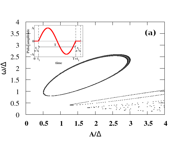
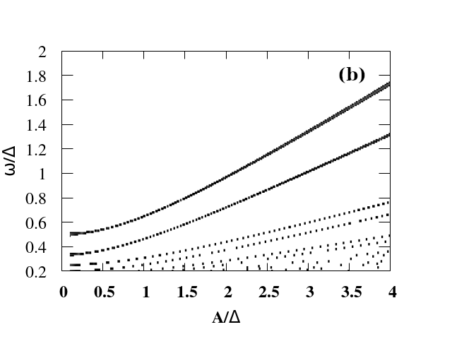
Figure 4: (a) Plot of the parameter sets $\omega$ and $A$ for the implementation of $X_{\frac{\pi}{2}}$ and $Y_{\frac{\pi}{2}}$ gates, obtained from the analytical expressions of Eqs.(17) and (22) (except for the low frequency points, that correspond to the numerical evaluation of the condition $P_{01}=1/2$). See text for details. Inset: Schematic representation of the pulsing protocol with an idle time $t_{i}$ added before the sinusoidal drive and a second idle time $t_{f}$ afterwards. (b) Values of $\omega$ and $A$ to implement the identity operation determined from Eq.(23).

The problem with the above conditions, Eqs.(14) and (16), is that each one requires very specific (and different) frequencies ($\omega_{Y}$ and $\omega_{X}$) and gate times ($T_{Y}=2\pi/\omega_{Y}$ and $T_{X}=2\pi/\omega_{X}$) to implement them.

A more general procedure McKay et al. (2017); Campbell et al. (2020), that expands the possibilities in parameter space, is to add an idle time $t_{i}$ before the sinusoidal drive and a second idle time $t_{f}$ afterwards, see inset in Fig.4(a). Calling $\tau_{+}=(t_{i}+t_{f})\Delta/2$ and $\tau_{-}=(t_{f}-t_{i})\Delta/2$, the evolution operator in the CHRW approximation results

$$U(t_{i}+T+t_{f})=$$

$$\!\!\!\!\!=\left(\!\begin{array}[]{cc}-e^{i\tau_{+}}(\cos\alpha+i\sin\alpha\cos{\tilde{\theta}})&-e^{i\tau_{-}}\sin\alpha\sin{\tilde{\theta}}\\ e^{-i\tau_{-}}\sin\alpha\sin{\tilde{\theta}}&-e^{-i\tau_{+}}(\cos\alpha-i\sin\alpha\cos{\tilde{\theta}})\end{array}\!\!\!\right)\!.$$

For both gates, $X_{\frac{\pi}{2}}$ and $Y_{\frac{\pi}{2}}$, the transition probability after one period is $P_{01}=|\langle 1|U|0\rangle|^{2}=1/2$, which corresponds to the implicit condition for $\omega$ and $A$ given from the equation,

$$\sin{{}^{2}}{\tilde{\theta}}\sin{{}^{2}}\alpha=\frac{1}{2}.$$ (17)

Thus after imposing this condition in $U(t_{i}+T+t_{f})$ one gets

$$U(t_{i}+T+t_{f})=\frac{\sqrt{2}}{2}\left(\begin{array}[]{cc}-e^{i(\tau_{+}+\nu)}&-e^{i\tau_{-}}\\ e^{-i\tau_{-}}&-e^{-i(\tau_{+}+\nu)}\end{array}\right)$$ (18)

where

$$\tan\nu=\tan\alpha\cos{\tilde{\theta}}.$$ (19)

Then the $X_{\frac{\pi}{2}}$ gate can be obtained for

$$\tau_{-} = (2n+1/2)\pi$$

$$\tau_{+} = (2k+1)\pi-\nu,$$ (20)

being $k$ and $n$ integers, while the $Y_{\frac{\pi}{2}}$ gate can be implemented for

$$\tau_{-} = 2n\pi$$

$$\tau_{+} = (2k+1)\pi-\nu,$$ (21)

after straightforward comparisons with Eqs.(15) and (13), respectively.

To summarize, in order to determine the driving parameters $\omega,A,t_{i},t_{f}$ for the gate implementation one can proceed as follows. For a given driving frequency $\omega$ one determines the possible amplitudes $A$ solving Eq.(17). Notice that since the relevant solutions of Eq.(17) are for $\omega>A$, it is very accurate to use for the $\xi$ parameter the expression

$$\xi\approx\frac{\omega}{\omega+\Delta},$$ (22)

from a first order approximation of Eq.(5). The resulting curve in $A,\omega$ space is shown in Fig.4(a), where all the possible values for implementation of $X_{\frac{\pi}{2}}$ and $Y_{\frac{\pi}{2}}$ gates are plotted. We find that they fall within the range $\Delta\lesssim\omega<3\Delta$ and $\Delta/2\lesssim A<3\Delta$. (We also plot for completeness in Fig.4(a) the low frequency curves, for $\omega\ll A$, even when these cases are not of interest for the implementation of fast gates. These points were obtained from the evaluation of $P_{01}=|\langle 1|U_{num}|0\rangle|^{2}=1/2$ using the numerically exact evolution, since the CHRW approximation does not apply in this case.)

Once the chosen driving parameters $A,\omega$ are determined from Eq.(17), the values of the idling times $t_{i}$ and $t_{f}$ needed to implement a $X_{\frac{\pi}{2}}$ or a $Y_{\frac{\pi}{2}}$ gate can be obtained from Eqs.(20) or (21), respectively.

It has been argued in Ref.Weiss et al. (2022) that, since different physical qubits could have different $\Delta$ parameters, it is useful to have variable-time single qubit identity operations, to be able to perform operations in one qubit avoiding that a second qubit acquires a dynamical phase at the same time. Comparing the CHRW expression of $U(T)$ given in Eq.(10) with the identity matrix we obtain that the identity operation can be implemented for the $A,\omega$ that satisfy the simple condition

$$\omega=\Omega_{R}/(2k+1).$$ (23)

The resulting values of $A,\omega$ are shown in Fig.4(b), where we observe that in this case it is possible to use arbitrary large values of $\omega$ (and large $A$). On the other hand, for the $X_{\frac{\pi}{2}}$ and $Y_{\frac{\pi}{2}}$ gates one can see in Fig.4(a) that there is an upper limit in the frequency range for their implementation.

IV Two qubit gates

Any universal quantum instruction set requires the implementation of at least one entangling two-qubit gate Huang et al. (2023); Krantz et al. (2019); Kwon et al. (2021). Here we consider the parametrically driven two qubit Hamiltonian:

$$H_{2q}(t)=-\frac{\Delta_{1}}{2}\hat{\sigma}_{z}\otimes I-\frac{\Delta_{2}}{2}I\otimes\hat{\sigma}_{z}-\frac{\epsilon(t)}{2}\hat{\sigma}_{x}\otimes\hat{\sigma}_{x},$$ (24)

with driving in the coupling parameter $\epsilon(t)=A\sin(\omega t)$. Its matrix representation, using the basis $\left\{\left|00\right\rangle,\left|01\right\rangle,\left|10\right\rangle,\left|11\right\rangle\right\}$ is

$$H_{2q}(t)=-\frac{1}{2}\left(\begin{array}[]{cccc}\Delta_{1}+\Delta_{2}&0&0&\epsilon(t)\\ 0&\Delta_{1}-\Delta_{2}&\epsilon(t)&0\\ 0&\epsilon(t)&\Delta_{2}-\Delta_{1}&0\\ \epsilon(t)&0&0&-\Delta_{1}-\Delta_{2}\end{array}\right).$$

This two-qubit Hamiltonian with a $\hat{\sigma}_{x}\otimes\hat{\sigma}_{x}$ tunable coupling has been implemented for example in coupled fluxonium qubits Weiss et al. (2022); Moskalenko et al. (2021, 2022).

In the following we show that with a single period sinusoidal drive, it is straightforward to get the $\sqrt{\rm{bSWAP}}$ entangling gate Poletto et al. (2012); Roth et al. (2017); Nesterov et al. (2021):

$$U_{ent}=\sqrt{\rm{bSWAP}}=\left(\begin{array}[]{cccc}\frac{\sqrt{2}}{2}&0&0&-\frac{\sqrt{2}}{2}\\ 0&1&0&0\\ 0&0&1&0\\ \frac{\sqrt{2}}{2}&0&0&\frac{\sqrt{2}}{2}\end{array}\right),$$ (25)

which generates the entangled states $(|00\rangle\pm|11\rangle)/\sqrt{2}$ and leaves invariant the subspace spanned by $\{|01\rangle,|10\rangle\}$. It is easy to show that it is locally equivalent to the $\sqrt{\rm{iSWAP}}$ gate Poletto et al. (2012); Huang et al. (2023).

The $\sqrt{\rm{bSWAP}}$ gate can be exactly implemented in the ideal case when both qubits have equal gaps, $\Delta_{1}=\Delta_{2}=\Delta$. To demonstrate its realization, we calculate the error function ${\cal E}$ of the exact evolution operator $U_{num,2q}(T)$, computed numerically from $H_{2q}(t)$, compared with the target gate $U_{tg}=U_{ent}$, as a function of the parameters $\omega$ and $A$. In the plot of Fig.5(a) we find a point $A_{bS},\omega_{bS}$ with a minimum ${\cal E}$, near the numerical accuracy, which shows that it is possible to implement the $\sqrt{\rm{bSWAP}}$ gate with this protocol. To illustrate the dynamical process that leads to the $\sqrt{\rm{bSWAP}}$ gate, we show in Fig.5(b) the time evolution of the population transfers during a driving period at $\omega_{bS},A_{bS}$. Furthermore, in Fig.5(c) we see that in a non ideal case, when there is a small difference in the gaps of the qubits, $\Delta_{2}=1.05\Delta_{1}$, the $\sqrt{\rm{bSWAP}}$ gate can be reproduced at a slightly shifted operational point and with error ${\cal E}\approx 10^{-6}$.

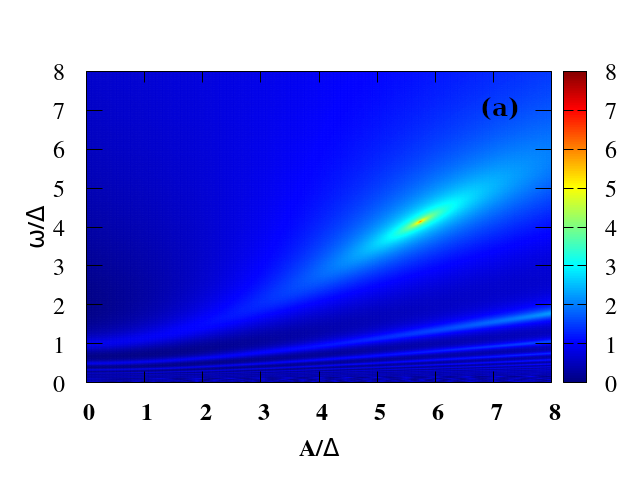
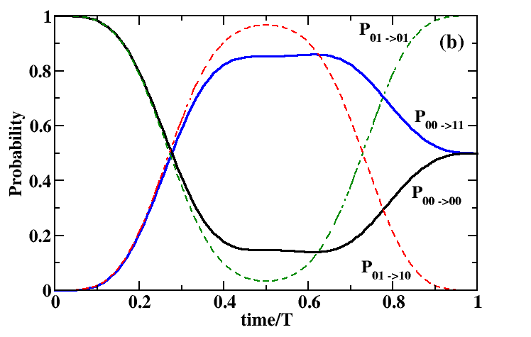
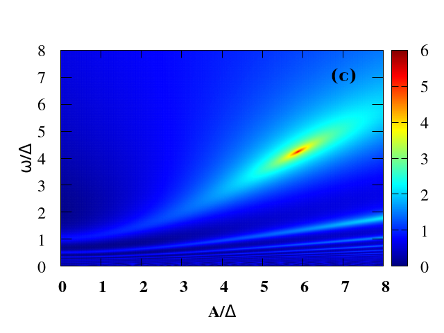
Figure 5: (a) Plot, as a function of the parameters $A$ and $\omega$, of the error ${\cal E}$ that compares $\sqrt{\rm{bSWAP}}$ with the numerically exact $U_{num,2q}$, computed from $H_{2q}$ Eq.(24). The color scale of the intensity plot corresponds to $-\log_{10}|{\cal E}|$. The point where ${\cal E}<10^{-7}$ (practically zero within numerical precision) gives the operational parameters of the gate, frequency $\omega_{bS}$ and amplitude $A_{bS}$. It agrees with the analytical estimate of $\omega_{bS}\approx 4.14\Delta$, $A_{bS}\approx 5.74\Delta$. (b) Time evolution of the population transfers during a driving period for $\omega_{bS},A_{bS}$. Continuous lines correspond to the evolution of the populations of the $|00\rangle$ (black) and the $|11\rangle$ states (blue), after the initial state $|00\rangle$. Dashed lines correspond to the evolution of the populations of the $|01\rangle$ (green) and the $|10\rangle$ states (red), after the initial state $|01\rangle$. (c) Same as (a) but for two slightly different qubits with $\Delta_{2}=1.05\Delta_{1}$. See text for more details.

We can proceed as in the previous section and provide an analytical estimate of the parameters for the $\sqrt{\rm{bSWAP}}$. To use the CHRW approximation of Sec.II it is convenient to transform $H_{2q}(t)$ to $\widetilde{H_{2q}}=SH_{2q}S^{\dagger}$ with

$$S=\left(\begin{array}[]{cccc}1&0&0&0\\ 0&0&0&1\\ 0&0&1&0\\ 0&1&0&0\end{array}\right),$$

obtaining

$$\widetilde{H_{2q}}(t)=-\frac{1}{2}\left(\begin{array}[]{cccc}\Delta_{1}+\Delta_{2}&\epsilon(t)&0&0\\ \epsilon(t)&-\Delta_{1}-\Delta_{2}&0&0\\ 0&0&\Delta_{2}-\Delta_{1}&\epsilon(t)\\ 0&0&\epsilon(t)&\Delta_{1}-\Delta_{2}\end{array}\right),$$

which separates in two independent blocks,

$$\widetilde{H_{2q}}(t) = \left[-\frac{\Delta_{+}}{2}\hat{\sigma}_{z}-\frac{\epsilon(t)}{2}\hat{\sigma}_{x}\right]\otimes\left(\begin{array}[]{cc}1&0\\ 0&0\end{array}\right)$$ (28)

$$+ \left[-\frac{\Delta_{-}}{2}\hat{\sigma}_{z}-\frac{\epsilon(t)}{2}\hat{\sigma}_{x}\right]\otimes\left(\begin{array}[]{cc}0&0\\ 0&1\end{array}\right),$$ (31)

with $\Delta_{+}=\Delta_{1}+\Delta_{2}$ and $\Delta_{-}=\Delta_{2}-\Delta_{1}$. Thus, in this basis we can express the evolution operator $\widetilde{U_{2q}}$ in terms of single qubit operators as,

$$\widetilde{U_{2q}}(t)=U_{+}(t)\otimes\left(\begin{array}[]{cc}1&0\\ 0&0\end{array}\right)+U_{-}(t)\otimes\left(\begin{array}[]{cc}0&0\\ 0&1\end{array}\right),$$ (32)

where $U_{+}$ ($U_{-}$) is equal to the single qubit evolution operator after replacing $\Delta$ by $\Delta_{+}$ ($\Delta_{-}$). It is now straightforward to obtain the evolution operator in the CHRW approximation, following the same steps as in the single qubit case for $U_{+}$ and $U_{-}$. After one period $T$, and transforming back to the original basis, we obtain

$$U_{2q}(T)=-\left(\begin{array}[]{cccc}a_{+}&0&0&b_{+}\\ 0&a_{-}^{*}&b_{-}&0\\ 0&-b_{-}&a_{-}&0\\ -b_{+}&0&0&a_{+}^{*}\end{array}\right),$$ (33)

with

$$a_{+} = \cos\alpha_{+}+i\sin\alpha_{+}\cos{\widetilde{\theta}}_{+}$$

$$b_{+} = \sin\alpha_{+}\sin{\widetilde{\theta}}_{+}$$

$$a_{-} = \cos\alpha_{-}+i\sin\alpha_{-}\cos{\widetilde{\theta}}_{-}$$

$$b_{-} = \sin\alpha_{-}\sin{\widetilde{\theta}}_{-},$$

where $\alpha_{+(-)},{\widetilde{\theta}}_{+(-)}$ are obtained as in Sec.II after replacing $\Delta\rightarrow\Delta_{+}(\Delta_{-})$ in the generalized Rabi frequency $\Omega_{R}\rightarrow\Omega_{+R}(\Omega_{-R})$ and $(..)^{*}$ denotes the complex conjugate operation.

When $\Delta_{\text{1}}$=$\Delta_{2}=\Delta$, since $\Delta_{-}=0$ , we have

$$U_{2q}(T)=\left(\begin{array}[]{cccc}-a_{+}&0&0&-b_{+}\\ 0&1&0&0\\ 0&0&1&0\\ b_{+}&0&0&-a_{+}^{*}\end{array}\right).$$ (34)

Therefore, to obtain the $\sqrt{\rm{bSWAP}}$ gate, a comparison with Eq.(25) gives $b_{+}=-a_{+}=\frac{\sqrt{2}}{2}$ with $\Delta_{+}=2\Delta$ and the main the conditions are:

$$\omega = \frac{4}{3}\Omega_{+R},$$ (35)

$$\theta_{+}-\xi_{+}\frac{A}{\omega} = \frac{\pi}{2}$$

Numerical solution of these equations give $\omega_{bS}=4.14\Delta$, $A_{bS}=5.74\Delta$, which coincide with the optimal point of Fig.5(a). (Note that they are the same as for the $Y_{\frac{\pi}{2}}$ gate after the substitution $\Delta\rightarrow 2\Delta$, an so similarly the general conditions can be obtained.)

As in the single qubit case, for the $\sqrt{\rm{bSWAP}}$ gate we can extend the set of parameters to those $A,\omega$ which satisfy $P_{00\rightarrow 11}=1/2$. It is straightforward to show that this set is obtained from the solution of:

$$P_{00\rightarrow 11} = |\langle 11|U_{2q}(T)|00\rangle|{{}^{2}}$$ (36)

$$= \sin{{}^{2}}{\tilde{\theta}_{+}}\sin{{}^{2}}\alpha_{+}=\frac{1}{2}.$$

To implement the $\sqrt{\rm{bSWAP}}$ gate for the parameters satisfying the above equation, one has to add an idle time $t_{i}$ before the sinusoidal drive and second idle time $t_{f}$ afterwards. Calling $\tau_{+}=(t_{1}+t_{2})\Delta$ , $\tau_{-}=(t_{2}-t_{1})\Delta$, we have

$$U(t_{i}+T+t_{f})=e^{i\frac{\tau_{2}}{2}(\hat{\sigma}_{z}\otimes I+I\otimes\hat{\sigma}_{z})}U(T)e^{i\frac{\tau_{1}}{2}(\hat{\sigma}_{z}\otimes I+I\otimes\hat{\sigma}_{z})}$$ (38)

$$=\left(\begin{array}[]{cccc}-e^{i\tau_{+}}a_{+}&0&0&-e^{i\tau_{-}}b_{+}\\ 0&1&0&0\\ 0&0&1&0\\ e^{-i\tau_{-}}b_{+}&0&0&-e^{-i\tau_{+}}a_{+}^{*}\end{array}\right).$$ (39)

Defining $\rho e^{i\nu}=\cos\alpha_{+}+i\sin\alpha_{+}\cos{\tilde{\theta}_{+}}$, where $\tan\nu=\tan\alpha_{+}\cos{\tilde{\theta}_{+}}$, we can write

$$\left(\begin{array}[]{cccc}-\rho e^{i(\tau_{+}+\nu)}&0&0&\mp e^{i\tau_{-}}\sqrt{1-\rho^{2}}\\ 0&1&0&0\\ 0&0&1&0\\ \pm e^{-i\tau_{-}}\sqrt{1-\rho^{2}}&0&0&-\rho e^{-i(\tau_{+}+\nu)}\end{array}\right).$$ (40)

For the case $P_{00\rightarrow 11}=1-\rho^{2}=1/2$ this corresponds to

$$\left(\begin{array}[]{cccc}\frac{\sqrt{2}}{2}e^{i(\tau_{+}+\nu)}&0&0&\mp\frac{\sqrt{2}}{2}e^{i\tau_{-}}\\ 0&1&0&0\\ 0&0&1&0\\ \pm\frac{\sqrt{2}}{2}e^{-i\tau_{-}}&0&0&\frac{\sqrt{2}}{2}e^{-i(\tau_{+}+\nu)}\end{array}\right).$$ (41)

Then the $\sqrt{\rm{bSWAP}}$ gate can be obtained for $\tau_{-}=2k\pi$ and $\tau_{+}+\nu=(2n+1)\pi$.

This gate is robust against a small difference in the parameters of the two qubits. For $\Delta_{2}-\Delta_{1}=\epsilon\Delta$, the invariance under gate operation of the subspace spanned by $\{|01\rangle,|10\rangle\}$ can not be attained exactly. Then, the error in the gate operation can be estimated from evaluating the probability $P_{|10\rangle\rightarrow|01\rangle}$, which should be zero for a perfect gate. For $\epsilon\ll 1$ we estimate the error from Eq.(33) as ${\cal E}_{\epsilon}\propto P_{|10\rangle\rightarrow|01\rangle}=b_{-}^{2}\approx\epsilon^{2}\pi^{2}(\frac{\Delta}{\omega})^{2}J_{0}^{2}(\frac{A}{\omega})\sin^{2}(\frac{A}{\omega})$. For the case $(A_{bS},\omega_{bS})$ and $\epsilon=0.01$ the error is ${\cal E}_{0.01}\approx 2\times 10^{-5}$ and it decreases as $\sim\omega^{-2}$ for increasing $\omega$.

V Relaxation and decoherence under strong drive

In the previous sections we have found more than one choice for the operational parameters $\omega,A$ to implement single qubit and two qubit gates with a LZSM protocol. In this section we analyze the effects of the environment on the gate dynamics since it is known that for strong driving the transition rates can depend on the driving parameters Kohler et al. (1998); Hausinger and Grifoni (2010a); Ferrón et al. (2012, 2016); Yan et al. (2013); Yoshihara et al. (2014). Therefore the dependence of relaxation and decoherence rates on $\omega,A$ has to be considered to fine tune the implementation of qubit gates under these protocols. We will discuss here the single qubit case, but the analysis can be extended straightforwardly for the case of two qubits considering that the dynamics of the Hamiltonian of Eq.(24), can be transformed to the dynamics of two independent qubits as shown in Eqs.(28) and (32).

The effect of the environment can be described by the global Hamiltonian ${\cal H}(t)={H}_{s}(t)+{H}_{b}+{H}_{sb}$, where ${H}_{s}(t)={H}_{s}(t+T)$ is the Hamiltonian of the driven qubits with time period $T=2\pi/\omega$. The Hamiltonian ${H}_{b}$ corresponds to a thermal bath and ${H}_{sb}=\hat{O}\otimes\hat{B}$ is the system-bath coupling term, with $\hat{B}$ representing the quantum noise due to the bath and $\hat{O}$ is the observable of the system coupled to the noise.

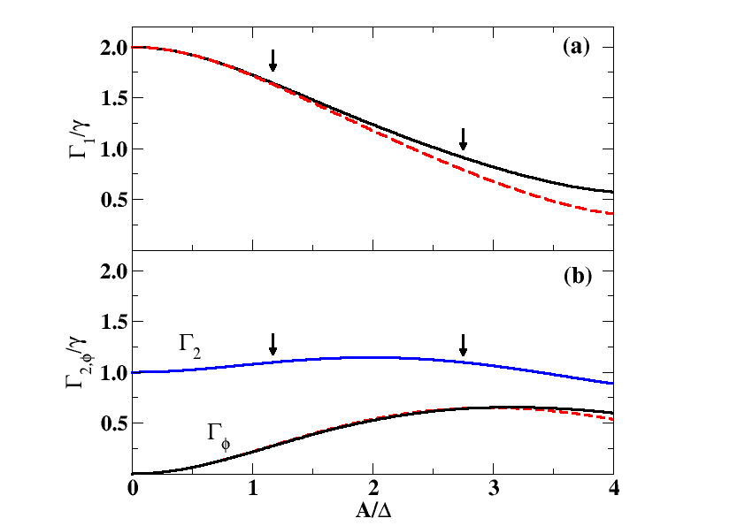
Figure 6: (a) Plot of the relaxation rate $\Gamma_{1}$ as a function of $A/\Delta$ for $\omega=1.92\Delta$. The black continuous line corresponds to the numerically exact value and the dashed line the CHRW approximation, Eq.(43). (b) Plot of the dephasing rate $\Gamma_{\phi}$ as a function of $A/\Delta$ for $\omega=1.92\Delta$. The black continuous line corresponds to the numerically exact value and the dashed line the CHRW approximation. Also the decoherence rate $\Gamma_{2}$ is plotted (blue continuous line, numerically exact values only). Both in (a) and (b): the arrows indicate the values of $A$ where the $X_{\frac{\pi}{2}}$, $Y_{\frac{\pi}{2}}$ gates can be implemented, as obtained from Fig.4(a); the rates $\Gamma_{1},\Gamma_{\phi},\Gamma_{2}$ are normalized by the noise strength parameter $\gamma$ and correspond to a thermal bath at temperature $T_{b}=0.1\Delta$.

The natural basis to compute relaxation and decoherence rates in the case of strong time periodic drives is the Floquet basis Shirley (1965), since in this basis the density matrix in the steady state becomes diagonal Grifoni and Hänggi (1998); Hausinger and Grifoni (2010b); Kohler et al. (1997, 1998); Breuer et al. (2000); Hone et al. (2009); Ferrón et al. (2016); Gasparinetti et al. (2013, 2014). In the case of the two level system, like the Hamiltonian of Eq.(1), the wave functions have the time dependence $|\Psi(t)\rangle=c_{a}e^{-i\epsilon_{a}t}|a(t)\rangle+c_{b}e^{-i\epsilon_{b}t}|b(t)\rangle$, where the Floquet states $|a(t)\rangle$, $|b(t)\rangle$ are periodic with time period $T$, and $\epsilon_{a}$, $\epsilon_{b}$ are the associated quasienergies Shirley (1965); Grifoni and Hänggi (1998); Hausinger and Grifoni (2010b); Ferrón and Domínguez (2010). In the CHRW approximation, $|a(t)\rangle$ and $|b(t)\rangle$ can be obtained from the eigenstates of the static Hamiltonian, Eq.(7), after performing on them a time dependent transformation back to the representation of the original Hamiltonian Eq.(1). In the limit $A\rightarrow 0$ the Floquet states tend to the eigenstates of the undriven Hamiltonian: $|a(t)\rangle\rightarrow|0\rangle$, $|b(t)\rangle\rightarrow|1\rangle$, and similarly the Floquet gap $\Delta_{F}=|\epsilon_{b}-\epsilon_{a}|$ tends to the undriven gap, $\Delta_{F}\rightarrow\Delta=E_{1}-E_{0}$.

From the Floquet-Markov quantum master equation (see Appendix A) the relaxation rate can be obtained as,

$$\Gamma_{1} = \sum_{q}S(\epsilon_{b}-\epsilon_{a}+q\omega)\left|\frac{1}{T}\int_{0}^{T}\langle a(t)|\hat{O}|b(t)\rangle e^{iq\omega t}dt\right|^{2}$$ (42)

$$\approx S(\Delta_{F})\left|\frac{1}{T}\int_{0}^{T}\langle a(t)|\hat{O}|b(t)\rangle dt\right|^{2},$$

where $S(\Omega)$ is the noise power spectrum. The second line of Eq.(42) approximates $\Gamma_{1}$ with the $q=0$ term, which is the dominant contribution in the sum of the first line. It is also direct to show that in the undriven limit, $A\rightarrow 0$, we can recover the standard result $\Gamma_{1}=S(\Delta)|\langle 0|\hat{O}|1\rangle|^{2}$.

We consider here that the main source of quantum noise is through the same channel as the driving, and thus we take for the noise coupling operator $\hat{O}=\hat{\sigma}_{x}$. An approximate expression of $\Gamma_{1}$ can be obtained calculating the matrix elements $\langle a(t)|\hat{\sigma}_{x}|b(t)\rangle$ in the CHRW approximation (see Appendix A),

$$\Gamma_{1}\approx S(\Delta_{F})\cos^{4}\frac{\theta}{2}.$$ (43)

where $\Delta_{F}=|\Omega_{R}-\omega|$ in this case. We have calculated the dependence of $\Gamma_{1}$ with the frequency $\omega$ and the amplitude $A$ considering noise with power spectrum $S(\Omega)=2\gamma\Omega\coth({\Omega}/{2T_{b}})$. We obtain the values of $\Gamma_{1}$ normalized by the noise strength parameter $\gamma$. In order to see more clearly the dependence with the driving parameters, we show the case for a low temperature $T_{b}=0.1\Delta$. We find that the general behavior for $\omega>\Delta$ is that the relaxation rate decreases with increasing $A$, as seen in Fig.6(a) for frequency $\omega=1.96\Delta$ in the range of interest com . Higher temperatures ($T_{b}\gtrsim\Delta$) give a similar behavior but with a milder dependence with $A$. The arrows in Fig.6(a) indicate the values of $A$ for which the $X_{\frac{\pi}{2}}$, $Y_{\frac{\pi}{2}}$ gates could be implemented at this driving frequency, as obtained from Fig.4(a). Considering that $\Gamma_{1}$ is smaller for larger $A$, the value indicated by the second arrow in the plot should be the preferred choice for a reduced effect of the environment in the qubit dynamics. We also plot in Fig.6(a) the CHRW approximation of Eq.(43) and the numerically exact evaluation of Eq.(42) (after calculating the Floquet states and quasienergies and summing terms in $q$ up $\pm 32$), showing that they are in good agreement.

To complete the analysis of the effect of the environment, we have to calculate the decoherence rate $\Gamma_{2}={\Gamma_{1}}/{2}+\Gamma_{\phi}$. The dephasing rate $\Gamma_{\phi}$ can be obtained from the Floquet-Markov quantum master equation as

$$\Gamma_{\phi}=\sum_{q\geq 0}2S(q\omega)\left|\frac{1}{T}\int_{0}^{T}dt\langle a(t)|\hat{O}|a(t)\rangle e^{iq\omega t}\right|^{2}.$$ (44)

In the case under consideration, with noise coupling operator $\hat{O}=\hat{\sigma}_{x}$, the $q=0$ term is exactly zero. Moreover, in the undriven limit $A\rightarrow 0$ the dephasing rate completely vanishes, $\Gamma_{\phi}^{A\rightarrow 0}=0$, corresponding to the fact that the qubit of Eq.(1) is in a ”sweet spot” Campbell et al. (2020). But, for finite driving, the $q\not=0$ terms start to contribute to dephasing with the dominant term being the $q=1$ term, leading to the expression

$$\Gamma_{\phi}\approx 2S(\omega)\left|\frac{1}{T}\int_{0}^{T}dt\langle a(t)|\hat{\sigma}_{x}|a(t)\rangle e^{i\omega t}\right|^{2}.$$ (45)

In this case, the CHRW approximation gives

$$\Gamma_{\phi}\approx 2S(\omega)[\sin\theta(J_{0}+J_{2})+\sin^{2}\frac{\theta}{2}(J_{1}+J_{3})]^{2},$$ (46)

where we have denoted $J_{l}\equiv J_{l}(\xi A/\omega)$. We plot in Fig.6(b) the dephasing rate $\Gamma_{\phi}$ as a function of $A$ for $\omega=1.96\Delta$. As stated, we find that $\Gamma_{\phi}=0$ for $A=0$, and then that $\Gamma_{\phi}$ increases for increasing $A$. Therefore dephasing is increased by the driving, which is in the opposite direction as the effect of driving on the relaxation rate, analyzed in the previous paragraph. However, to determine the optimal parameters for the gate, one has to analyze the decoherence rate $\Gamma_{2}$, that combines dephasing and relaxation. As can be seen in Fig.6(b), the decoherence rate changes mildly as a function of the driving strength $A$, being nearly the same for the two cases indicated by the arrows. Therefore, considering the previously discussed driving effect on relaxation, the larger $A$ is still the better choice for the implementation of the gates. We also compare in Fig.6(b) the approximated and the numerically exact $\Gamma_{\phi}$, which are in good agreement.

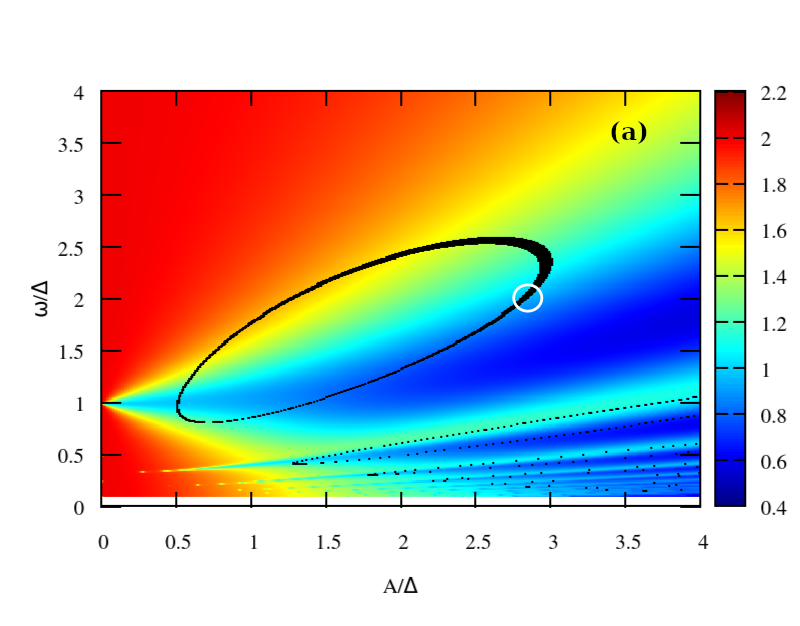
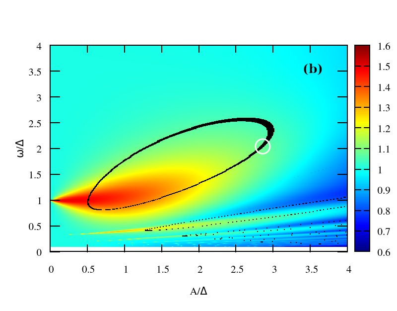
Figure 7: Intensity plot of (a) the relaxation rate $\Gamma_{1}$ and (b) the decoherence rate $\Gamma_{2}$, as a function of $A/\Delta$ and $\omega/\Delta$. The black dots indicate the parameter sets $\omega$ and $A$ for the implementation of $X_{\frac{\pi}{2}}$ and $Y_{\frac{\pi}{2}}$ gates, as in Fig.4(a). The white circle shows the optimal parameter region to minimize environmental effects. The rates $\Gamma_{1},\Gamma_{2}$ are normalized by the noise strength parameter $\gamma$ and correspond to a thermal bath at temperature $T_{b}=0.1\Delta$.

When considering lower $\omega$ the behavior of $\Gamma_{1}$ and $\Gamma_{2}$ is more complex. In Fig.7(a) and (b) we show intensity plots of $\Gamma_{1}$ and $\Gamma_{2}$, respectively, as a function of $A$ and $\omega$, plotting the numerically exact values in the full range of $\omega$ (the approximated values discussed above are accurate only for $\omega>\Delta$). We also plot in Fig.7 (with black dots) the values of $A,\omega$ corresponding to the conditions for the implementation of the $X_{\frac{\pi}{2}}$, $Y_{\frac{\pi}{2}}$ gates. The relaxation rate $\Gamma_{1}$ decreases for increasing $A$ for any of the frequencies in the range of interest ($\omega\gtrsim\Delta$), thus large $A$ would be always more convenient for gate implementations in order to minimize relaxation. In the plot of Fig.7(a) this corresponds to the gate parameters that fall within the blue colored region (which indicates lowest values of $\Gamma_{1}$ in the color scale of the plot).

On the other hand, the decoherence rate $\Gamma_{2}$ is large in the regions near resonance $\omega\sim\Delta$ and for $A\lesssim 2\Delta$, within the red colored region in Fig.7(b). This behavior is almost independent of temperature, i.e., higher temperatures ($T_{b}\gtrsim\Delta$) give similar plots except for a larger overall value of $\Gamma_{2}$, because the relevant dependence is on the matrix element $\left|\frac{1}{T}\int_{0}^{T}dt\langle a(t)|\hat{\sigma}_{x}|a(t)\rangle e^{i\omega t}\right|^{2}$. Therefore, off-resonant large frequency driving is always more convenient for the gates analyzed here, since for $\omega\gg\Delta$ the decoherence rate is low and nearly insensitive to variations in the driving amplitude $A$.

The combined analysis of the competing conditions for minimal relaxation and minimal decoherence lead to the conclusion that the best parameters for the implementation of the $X_{\frac{\pi}{2}}$, $Y_{\frac{\pi}{2}}$ gates are within the region in ${A,\omega}$ highlighted with a circle in Fig.7.

VI Summary and Conclusions

We have analyzed LZSM strong driving protocols for the implementation of quantum gates which are well suited for small gap qubits. We provide accurate analytical equations to obtain the driving parameters (amplitude, frequency, initial and final idling times) for single qubit gates and for the $\sqrt{\rm{bSWAP}}$ two qubits gate. Our approach avoids the need to scan experimentally a wide range of parameters and instead it allows to focus in fine-tuning the device near the analytically predicted parameters.

We have found that the $X_{\frac{\pi}{2}}$ and $Y_{\frac{\pi}{2}}$ gates can be efficiently implemented with a single strong one-period sinusoidal drive, with parameters in the range $\Delta\lesssim\omega\lesssim 3\Delta$ and $\Delta\lesssim A\lesssim 3\Delta$. We note that the $X_{\frac{\pi}{2}}$ and $Y_{\frac{\pi}{2}}$ gates could also be implemented using a half-period sinusoidal drive, which would allow for operation at even larger amplitudes and frequencies (it is easy in the CHRW calculation to obtain the $U(T/2)$ operator and the corresponding conditions for the gates). However, a one-period sinusoidal drive is preferred since it has zero time integral and thus the dc components associated with pulse transients cancel out Campbell et al. (2020).

The high amplitude and high frequency of the sinusoidal pulses make necessary to take into account the dependence of relaxation and decoherence with the driving parameters. We have shown that relaxation and decoherence decrease with increasing amplitude. Therefore large $A$ should be preferred. However, leakage to higher energy levels could induce gate errors for large drives. This effect depends on the specific multilevel structure of the quantum device. A rule of thumb argument is that the amplitude $A$ should be smaller than $E_{2}-E_{1}$, with $E_{2}$ the energy of the third level (and $E_{0},E_{1}$ the qubit two-level energies), to avoid leakage effects. In the optimal region signaled in Fig.7 we find $A\sim 3\Delta$ for minimal relaxation and decoherence, then requiring $E_{2}-E_{1}\gg 3(E_{1}-E_{0})$. Most superconducting qubit devices fulfill this condition. Decoherence is much smaller in the off-resonant case, for frequencies $\omega>\Delta$. After one driving period $T$ the error due to relaxation is proportional to $\Gamma_{1}T=2\pi\Gamma_{1}/\omega$ and similarly the error due to decoherence is proportional to $2\pi\Gamma_{2}/\omega$. Therefore, high frequencies, which imply faster gates, are always preferred to reduce the detrimental effects of the environment.

Here we propose the $\sqrt{\rm{bSWAP}}$ gate as the simplest two-qubit gate that can be implemented with a strong driving LZSM protocol. Previous implementations of the $\sqrt{\rm{bSWAP}}$ gate have been with protocols based on two-photon transitions Poletto et al. (2012); Roth et al. (2017); Nesterov et al. (2021). The protocol based on LZSM transitions proposed here only requires a single one period sinusoidal pulse, and thus it can be easier to realize, and possibly faster, than the “two-photon” protocols. Therefore, we consider to be worthwhile to implement in the future this two-qubit gate in small gap superconducting qubits.

Acknowlegments

We acknowledge support from CNEA, CONICET , ANPCyT ( PICT2019-0654) and UNCuyo (06/C591).

Appendix A Floquet states and quantum master equation

A.1 Floquet states

Consider the two level Hamiltonian:

$$H(t)=-\frac{\Delta}{2}\hat{\sigma}_{z}-\frac{\epsilon(t)}{2}\hat{\sigma}_{x}$$ (47)

with $\epsilon(t)=A\sin(\omega t)$.

According to Floquet theorem for time-periodic Hamiltonians, the solutions of the Schrödinger equation are of the form $|\Psi_{\alpha}(t)\rangle=e^{i\epsilon_{\alpha}t/\hbar}|u_{\alpha}(t)\rangle$, where the Floquet states $|u_{\alpha}(t)\rangle$ satisfy $|u_{\alpha}(t)\rangle$=$|u_{\alpha}(t+T)\rangle$ and are eigenstates of $[{H}_{s}(t)-i\hbar\partial/\partial t]|u_{\alpha}(t)\rangle=\epsilon_{\alpha}|u_{\alpha}(t)\rangle$, with $\epsilon_{\alpha}$ the associated quasienergy Shirley (1965); Grifoni and Hänggi (1998); Hausinger and Grifoni (2010b). The evolution operator can be written in matrix form as

$$U(t)=P(t)e^{-iH_{F}t}P^{\dagger}(0)$$

where $P(t+T)=P(t)$ is the matrix that contains the components of the Floquet states (in a given basis). In the CHRW approximation we obtain for the matrix of Floquet states

$$P(t)=U_{x}^{\dagger}(t)R^{\dagger}(t)W^{\dagger}e^{i\frac{\omega t}{2}\hat{\sigma}_{z}}$$

where we have taken for $H_{F}$ the form:

$$H_{F}=-\frac{\Omega_{R}-\omega}{2}\hat{\sigma}_{z}$$

which gives the correct $\omega\rightarrow\infty$ limit.

From the columns of the $P(t)$ matrix we obtain the Floquet states

$$\left|u_{\alpha}(t)\right\rangle=\left\{\begin{array}[]{c}\left|a\right\rangle=\left(\begin{array}[]{c}\cos\frac{\theta}{2}\cos\frac{\phi}{2}-e^{-i\omega t}\sin\frac{\theta}{2}\sin\frac{\phi}{2}\\ i\cos\frac{\theta}{2}\sin\frac{\phi}{2}+ie^{i\omega t}\sin\frac{\theta}{2}\cos\frac{\phi}{2}\end{array}\right)\\ \\ \left|b\right\rangle=\left(\begin{array}[]{c}i\cos\frac{\theta}{2}\sin\frac{\phi}{2}+ie^{-i\omega t}\sin\frac{\theta}{2}\cos\frac{\phi}{2}\\ \cos\frac{\theta}{2}\cos\frac{\phi}{2}-e^{i\omega t}\sin\frac{\theta}{2}\sin\frac{\phi}{2}\end{array}\right)\end{array}\right.,$$

where $\theta=-\arctan{\widetilde{A}/\widetilde{\delta}}$ and $\phi(t)=-\xi\frac{A}{\omega}\cos(\omega t)$ were already defined in Sec.II. The corresponding quasienergies are

$$\epsilon_{a/b}=\mp\frac{\Omega_{R}-\omega}{2},$$

and the so called Floquet gap is $\Delta_{F}=|\epsilon_{b}-\epsilon_{a}|=|\Omega_{R}-\omega|$.

A.2 Floquet-Markov master equation and transition rates

The open system dynamics can be described by the global Hamiltonian ${\cal H}(t)={H}_{s}(t)+{H}_{b}+{H}_{sb}$, where ${H}_{s}(t)={H}_{s}(t+T)$ is the Hamiltonian of the qubits driven by periodic external fields with time period $T=2\pi/\omega$. The Hamiltonian ${H}_{b}$ corresponds to a bosonic thermal bath at temperature $T_{b}$ and spectral density $J(\Omega)$. The bath h is linearly coupled to the qubit system in the form ${H}_{sb}=\hat{O}\otimes\hat{B}$, with $\hat{B}$ an observable of the bath and $\hat{O}$ an observable of the system. After performing the Born and Markov approximations, a quantum master equation can be obtained Grifoni and Hänggi (1998); Hausinger and Grifoni (2010b); Kohler et al. (1997, 1998); Breuer et al. (2000); Hone et al. (2009); Ferrón et al. (2016); Gasparinetti et al. (2013, 2014). In most situations (away from resonances) an additional secular approximation can be realized Grifoni and Hänggi (1998); Hausinger and Grifoni (2010b); Kohler et al. (1997, 1998); Breuer et al. (2000); Hone et al. (2009); Ferrón et al. (2016); Gasparinetti et al. (2013, 2014); Gramajo et al. (2018), leading to the quantum master equation:

$$\dot{\rho} =-i[H_{s}(t),\rho]+\sum_{\alpha\beta}\Gamma_{\alpha\beta}\left(L_{\alpha\beta}\rho L^{{\dagger}}_{\alpha\beta}-\frac{1}{2}\{L^{{\dagger}}_{\alpha\beta}L_{\alpha\beta},\rho\}\right),$$ (48)

where $L_{\alpha\beta}=|u_{\alpha}(t)\rangle\langle u_{\beta}(t)|$ are the corresponding jump operators, and the transition rates $\Gamma_{\alpha\beta}$ can be written as

$$\Gamma_{\alpha\beta}=\sum_{q}g(\epsilon_{\alpha\beta,q})|O_{\alpha\beta}(q)|^{2},$$ (49)

where the $q$-Fourier components of the transition matrix elements are

$$O_{\alpha\beta}(q)=\frac{1}{T}\int_{0}^{T}dt\langle u_{\alpha}(t)|\hat{O}|u_{\beta}(t)\rangle e^{iq\omega t},$$

and $g(x)$ is the spectral bath correlation function, $g(x)=J(x)n_{\rm th}(x)$ with with $J(x)$ the spectral density, $n_{\rm th}(x)=(\exp{(x/k_{B}T)}-1)^{-1}$, and $\varepsilon_{\alpha\beta,q}=\varepsilon_{\alpha}-\varepsilon_{\beta}+q\hbar\omega$.

In the case of a two-level system like the Hamiltonian of Eq.(47) the relaxation rate can be obtained from the Eq.(48) as

$$\Gamma_{1}=\sum_{q}g(\epsilon_{ab,q})|O_{ab}(q)|^{2}+g(\epsilon_{ba,q})|O_{ba}(q)|^{2}$$

Using that $O_{ab}(q)=\left[O_{ba}(-q)\right]^{*}$ we can write

$$\Gamma_{1}=\sum_{q}S(\epsilon_{ab,q})|O_{ab}(q)|^{2}$$

where $S(\Omega)$ is the noise power spectrum, $S(\Omega)=g(\Omega)+g(-\Omega)$. The decoherence rate is $\Gamma_{2}=\frac{\Gamma_{1}}{2}+\Gamma_{\phi}$ with the dephasing rate,

$$\Gamma_{\phi}=\sum_{q}g(q\omega)|O_{aa}(q)-O_{bb}(q)|^{2}$$

Without loss of generality we can choose ${\rm Tr}({\hat{O}})=0$, and then $O_{aa}(q)=-O_{bb}(q)$, giving

$$\Gamma_{\phi}=\sum_{q\geq 0}2S(q\omega)|O_{aa}(q)|^{2}$$

For $\hat{O}=\hat{\sigma}_{x}$ the matrix elements are $\langle u_{\alpha}(t)|\hat{O}|u_{\beta}(t)\rangle=\left\langle u_{\alpha}(t)|\hat{\sigma}_{x}|\beta(t)\right\rangle\equiv X_{\alpha\beta}(t)$. In the CHRW approximation we obtain the expressions

$$X_{ab}(t) = \cos{{}^{2}}\frac{\theta}{2}+\sin{{}^{2}}\frac{\theta}{2}\cos 2\omega t$$

$$-i\left(\sin\omega t\sin\theta\sin\phi+\sin 2\omega t\cos\phi\right)$$

$$X_{aa}(t)=-\sin\omega t\sin\theta\cos\phi+\sin 2\omega t\sin{{}^{2}}\frac{\theta}{2}\sin\phi$$

To evaluate the rates, the $q$ Fourier components $X_{\alpha\beta}(q)$ have to be calculated. After using the expansions for $\sin\phi(t)$ and $\cos\phi(t)$

$$\sin\phi(t)=\sum_{l}(-1)^{l+1}J_{2l+1}e^{i(2l+1)\omega t}$$

$$\cos\phi(t)=\sum_{l}(-1)^{l}J_{2l}e^{i2l\omega t}$$

with $J_{l}\equiv J_{l}(\xi A/\omega)$, we have,

$$X_{ab}(2l+1) = 0$$

$$X_{ab}(2l) = \frac{(-1)^{l+1}}{2}\left[\sin\theta\left(J_{2l+1}+J_{2l-1}\right)\right.$$

$$\left.-J_{2l-2}+J_{2l+2}\right]$$

$$+\delta_{l,0}\cos{{}^{2}}\frac{\theta}{2}+\left(\frac{\delta_{l,1}+\delta_{l,-1}}{2}\right)\sin{{}^{2}}\frac{\theta}{2}$$

$$X_{aa}(2l+1) = \frac{i^{2l+1}}{2}\left[\sin\theta\left(J_{2l}+J_{2l+2}\right)\right.$$

$$\left.-\sin{{}^{2}}\frac{\theta}{2}\left(J_{2l-1}-J_{2l+3}\right)\right]$$

$$X_{aa}(2l) = 0.$$

In the lowest approximation the relaxation rate is dominated by the $q=0$ term, giving

$$\Gamma_{1}\approx 2S(\Delta_{F})|X_{ab}(0)|^{2}=2S(\Delta_{F})\cos^{4}\frac{\theta}{2},$$

where the noise spectrum is evaluated at the Floquet gap $\Delta_{F}=|\Omega_{R}-\omega|$. On the other hand, for the dephasing rate, the $q=0$ term is zero, and we have to take the next term as an approximation,

$$\Gamma_{\phi}\approx 2S(\omega)|X_{aa}(1)|^{2}=S(\omega)[(J_{0}+J_{2})\sin\theta+(J_{1}+J_{3})\sin^{2}\frac{\theta}{2}]^{2}$$

Appendix B Other approximation methods to the dynamics

The dynamics of the driven two level system has been studied extensively along the last years. Different approximation methods have been attempted to solve the dynamics of a strongly driven qubit, given by the Hamiltonian Eq.(1) for $\epsilon(t)=A\sin(\omega t)$. Here we review some and compare them with the CHRW approximation.

B.1 Double rotating frame rotating wave approximation (DR)

The dynamics can also be approximated following the approach of Refs.Deng et al. (2015, 2016) where an improved (“second order”) rotating wave approximation is performed to calculate the Floquet states and quasienergies, after a basis transformation to a rotating frame with a time-dependent rotation frequency and a truncation of the transformed Floquet Hamiltonian to a 2 × 2 matrix.

Here we obtain the same result following a different (but equivalent) procedure, where we perform two rotation transformations of the Hamiltonian Eq.(1) and a RWA approximation at the end. We start with the $x$-rotation $|\psi^{\prime}(t)\rangle=U_{x}|\psi(t)\rangle$, with $U_{x}=e^{-i\frac{\phi}{2}\hat{\sigma}_{x}}$, and $\phi(t)=-\frac{A}{\omega}\cos(\omega t)$. After the rotation, the transformed Hamiltonian is $H^{\prime}=U_{x}HU_{x}^{\dagger}+i(\partial_{t}U_{x})U_{x}^{\dagger}$ and thus,

$$H^{\prime}=-\frac{\Delta}{2}(\cos\phi\hat{\sigma}_{z}-\sin\phi\hat{\sigma_{y}}).$$ (50)

Using the expansion of $e^{i\phi(t)}$ in terms of Bessel functions we approximate in Eq.(50) (neglecting the high frequency terms):

$$\cos\phi \approx J_{0}(\frac{A}{\omega})$$

$$\sin\phi \approx -2J_{1}(\frac{A}{\omega})\cos(\omega t),$$ (51)

and therefore

$$H^{\prime}=-\frac{\Delta}{2}\left[J_{0}(\frac{A}{\omega})\hat{\sigma}_{z}+2J_{1}(\frac{A}{\omega})\cos(\omega t)\hat{\sigma_{y}}\right].$$

The second rotation is a $z$-rotation with the unitary operator $U_{z}=e^{-i\frac{\omega t}{2}\hat{\sigma}_{z}}$, for which we obtain:

$$H^{\prime\prime}=-\frac{\widetilde{\delta}}{2}\hat{\sigma}_{z}+\frac{\widetilde{\nu}}{2}\left[(1+\cos 2\omega t)\hat{\sigma_{y}}-\sin 2\omega t\hat{\sigma_{x}}\right],$$ (52)

being $\widetilde{\delta}=\Delta J_{0}(a)-\omega$, $\widetilde{\nu}=\Delta J_{1}(\frac{A}{\omega})$ and $a=A/\omega$. Neglecting the fast oscillating terms with frequency $2\omega$ (RWA approximation),

$$H^{\prime\prime}\approx-\frac{\widetilde{\delta}}{2}\hat{\sigma}_{z}+\frac{\widetilde{\nu}}{2}\hat{\sigma_{y}}.$$ (53)

Equation (53) can be easily diagonalized with the transformation $W=e^{-i\frac{\theta}{2}\hat{\sigma}_{x}}$, being $\tan\theta=-\widetilde{\nu}/\widetilde{\delta}$, obtaining:

$$H_{d}=WH^{\prime\prime}W^{\dagger}=-\frac{\Omega_{R}}{2}\hat{\sigma}_{z},$$ (54)

with

$$\Omega_{R}=\sqrt{\widetilde{\delta}{{}^{2}}+\widetilde{\nu}{{}^{2}}}=\sqrt{[\Delta J_{0}(\frac{A}{\omega})-\omega]^{2}+\Delta^{2}J_{1}{{}^{2}}(\frac{A}{\omega})},$$

the generalized Rabi frequency.

Taking into account the previous transformations, the evolution operator associated to Eq.(1) results :

$$U^{DR}(t)=U_{x}^{\dagger}(t)U_{z}^{\dagger}(t)W^{\dagger}e^{i\frac{\Omega_{R}t}{2}\hat{\sigma}_{z}}WU_{z}(0)U_{x}(0),$$ (55)

which after one period of the driving, $T=2\pi/\omega$, is:

$$U^{DR}(T)=-e^{i\frac{\theta-a}{2}\hat{\sigma}_{x}}e^{i\frac{\pi\Omega_{R}}{\omega}\hat{\sigma}_{z}}e^{-i\frac{\theta-a}{2}\hat{\sigma}_{x}}$$ (56)

$$=-\left(\begin{array}[]{cc}\cos\alpha+i\sin\alpha\cos{\tilde{\theta}}&\sin\alpha\sin{\tilde{\theta}}\\ -\sin\alpha\sin{\tilde{\theta}}&\cos\alpha-i\sin\alpha\cos{\tilde{\theta}}\end{array}\right),$$

with $\alpha=\frac{\pi\Omega_{R}}{\omega}$ and ${\tilde{\theta}}=\theta-\frac{A}{\omega}$.

We can now calculate in this approximation the transition probability between the qubit states, $\left|0\right\rangle\rightarrow\left|1\right\rangle$ after a time $t=T$ as,

$$P_{01}^{DR}=|\langle 1|U(T)|0\rangle|{{}^{2}}=\sin{{}^{2}}{\tilde{\theta}}\sin{{}^{2}}\alpha$$ (57)

which is very similar in form to the obtained in the CHRW approximation. (Note that here the frequency $\Omega_{R}$ and the angles $\alpha$,$\theta$, etc. have different expressions).

B.2 Magnus expansion approximation (ME)

In Weiss et al. (2022) the dynamics is approximated with a Magnus expansion Magnus (1954); Blanes et al. (2009). Considering a Hamiltonian $H(t)$, the Magnus expansion for the evolution operator $U(t_{f},t_{i})$ from time $t=t_{i}$ to time $t=t_{f}$, with $\Delta t=t_{f}-t_{i}$, is

$$U\left(t_{f},t_{i}\right)=\exp\{-\mathrm{i}\bar{H}\Delta t\},$$ (58)

with

$$\bar{H}=\bar{H}^{(1)}+\bar{H}^{(2)}+\bar{H}^{(3)}+\bar{H}^{(4)}+\ldots\;,$$ (59)

where the first terms $\bar{H}^{(n)}$ of the expansion are:

$$\bar{H}^{(1)}= \frac{1}{\Delta t}\int_{t_{i}}^{t_{f}}\mathrm{~{}d}tH(t),$$ (60)

$$\bar{H}^{(2)}= \frac{1}{2\mathrm{i}\Delta t}\int_{t_{i}}^{t_{f}}\mathrm{~{}d}t\int_{t_{i}}^{t}\mathrm{~{}d}t^{\prime}\left[H(t),H\left(t^{\prime}\right)\right].$$

Since for fast gates we are interested in the evolution after one period of the drive $T=2\pi/\omega$, the Magnus expansion can be used to estimate $U(T)$ for the Hamiltonian $H$ given in Eq.(1). Following the approach of Weiss et al. (2022), we start by applying the transformations $|\psi^{\prime}(t)\rangle=U_{0}|\psi(t)\rangle$, $H^{\prime}=U_{0}HU_{0}^{\dagger}+i(\partial_{t}U_{0})U_{0}^{\dagger}$, with $U_{0}=e^{-i\frac{\chi}{2}\hat{\sigma}_{x}}$, and $\chi(t)=-\frac{A}{\omega}[\cos(\omega t)-1]$. This gives

$$H^{\prime}=-\frac{\Delta}{2}(\cos\chi\hat{\sigma}_{z}-\sin\chi\hat{\sigma_{y}}).$$ (61)

For the evolution after one period $T=2\pi/\omega$ we consider the lowest order in the Magnus expansion:

$$U^{\prime}(T)\approx e^{-i\frac{1}{T}\int_{0}^{T}\mathrm{~{}d}tH^{\prime}(t)}.$$

The Magnus expansion converges for $\|H(t)\|\Delta t\ll 1$, which in this case corresponds to the high frequency limit $\Delta\ll\omega$. Thus one obtains Weiss et al. (2022)

$$U^{\prime}(T)\approx-\left(\begin{array}[]{cc}\cos\alpha+i\sin\alpha\cos{\theta}&\sin\alpha\sin{\theta}\\ -\sin\alpha\sin{\theta}&\cos\alpha-i\sin\alpha\cos{\theta}\end{array}\right),$$

with $\alpha=\pi\Omega_{R}^{(0)}/\omega$, $\theta=A/\omega$, and $\Omega_{R}^{(0)}=\Delta J_{0}(\frac{A}{\omega})$. Since $U_{0}(0)=U_{0}(T)=I$, the evolution operator is $U(T)=U_{0}(T)U´(T)U_{0}^{\dagger}(0)=U^{\prime}(T)$. Therefore the transition probability $P_{01}$ in this first order Magnus expansion approximation is

$$P_{01}^{ME} = |\langle 1|U(T)|0\rangle|{{}^{2}}=\sin{{}^{2}}{\theta}\sin{{}^{2}}\alpha$$

$$= \sin^{2}(\frac{A}{\omega})\sin{{}^{2}}\frac{\pi\Delta J_{0}(\frac{A}{\omega})}{\omega}.$$

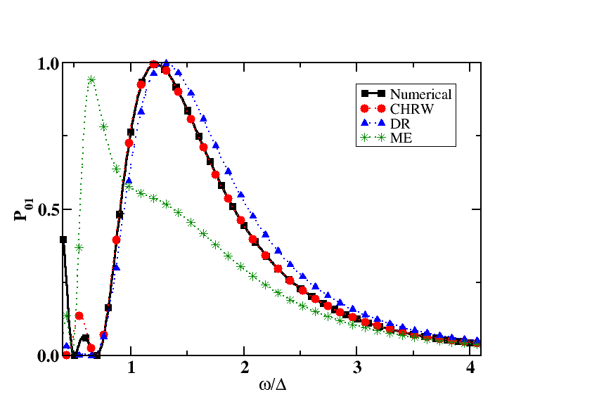
Figure 8: Plot of the transition probability $P_{01}$ as function of $\omega/\Delta$ for $A=1.16\Delta$ comparing different approximation methods. Black squares: numerically exact values. Red circles: counterrotating hybridized rotating wave approximation (CHRW), as given by Eq.(II). Blue triangles: double rotating frame rotating wave approximation (DR), as given by Eq.(57). Green stars: Magnus expansion approximation (ME), first order, as given by Eq.(B.2).

B.3 Comparison of the different approximations

We now compare the different approximations for the calculation of the transition probability $P_{01}$. In Fig.8 we show $P_{01}$ as a function of the frequency $\omega$ for $A=1.16\Delta$. We plot the numerically exact values obtained with a highly accurate fourth order Trotter-Suzuki algorithm Hatano and Suzuki (2005b). We find that the first order ME approximation of Eq.(B.2) only agrees with the exact results for $\omega\gtrsim 3\Delta$. On the other hand, the DR approximation of Eq.(57) agrees reasonably well with the exact dependence with frequency, with errors $\propto 10^{-2}$ in the frequencies of interest and improving accuracy for large frequencies.

The CHRW approximation is very accurate for $\omega\gtrsim\Delta$, and it is almost indistinguishable from the exact results in the scale of the plot. From Fig.2 one can see that for this amplitude and $\omega\gtrsim\Delta$ the error is ${\cal E}<10^{-5}$.

References

- Krantz et al. (2019) P. Krantz, M. Kjaergaard, F. Yan, T. P. Orlando, S. Gustavsson, and W. D. Oliver, Applied Physics Reviews 6, 021318 (2019).
- Kjaergaard et al. (2020) M. Kjaergaard, M. Schwartz, J. Braum”uller, P. Krantz, J. I.-J. Wang, S. Gustavsson, and W. Oliver, Annual Review of Condensed Matter Physics 11, 369 (2020).
- Kwon et al. (2021) S. Kwon, A. Tomonaga, G. Lakshmi Bhai, S. J. Devitt, and J.-S. Tsai, Journal of Applied Physics 129, 041102 (2021), https://pubs.aip.org/aip/jap/article-pdf/doi/10.1063/5.0029735/14770083/041102_1_online.pdf .
- Koch et al. (2007) J. Koch, T. Yu, M. Terri, J. Gambetta, A. A. Houck, D. I. Schuster, J. Majer, A. Blais, M. Devoret, S. Girvin, and R. J. Schoelkopf, Phys. Rev. A 76, 042319 (2007).
- Yan et al. (2016) F. Yan, S. Gustavsson, A. Kamal, J. Birenbaum, A. P. Sears, D. Hover, T. J. Gudmundsen, D. Rosenberg, G. Samach, S. Weber, et al., Nature communications 7, 1 (2016).
- Manucharyan et al. (2009) A. Manucharyan, J. Koch, L. I. Glazman, and M. H. Devoret, Science 326, 113 (2009).
- Pop et al. (2014) I. M. Pop, K. Geerlings, G. Catelani, R. J. Schoelkopf, L. I. Glazman, and M. H. Devoret, Nature 508, 369 (2014).
- Nguyen et al. (2019) L. B. Nguyen, Y.-H. Lin, A. Somoroff, R. Mencia, N. Grabon, and V. E. Manucharyan, Physical Review X 9, 041041 (2019).
- Bao et al. (2022) F. Bao, H. Deng, D. Ding, R. Gao, X. Gao, C. Huang, X. Jiang, H.-S. Ku, Z. Li, X. Ma, X. Ni, J. Qin, Z. Song, H. Sun, C. Tang, T. Wang, F. Wu, T. Xia, W. Yu, F. Zhang, G. Zhang, X. Zhang, J. Zhou, X. Zhu, Y. Shi, J. Chen, H.-H. Zhao, and C. Deng, Phys. Rev. Lett. 129, 010502 (2022).
- Weiss et al. (2022) D. K. Weiss, H. Zhang, C. Ding, Y. Ma, D. I. Schuster, and J. Koch, PRX Quantum 3, 040336 (2022).
- Somoroff et al. (2023) A. Somoroff, Q. Ficheux, R. A. Mencia, H. Xiong, R. Kuzmin, and V. E. Manucharyan, Phys. Rev. Lett. 130, 267001 (2023).
- Leek et al. (2007) P. J. Leek, J. M. Fink, A. Blais, R. Bianchetti, M. G”oppl, J. M. Gambetta, D. I. Schuster, L. Frunzio, R. J. Schoelkopf, and A. Wallraff, Science 318, 1889 (2007).
- Bylander et al. (2011) J. Bylander, S. Gustavsson, F. Yan, F. Yoshihara, K. Harrabi, G. Fitch, D. G. Cory, Y. Nakamura, J.-S. Tsai, and W. D. Oliver, Nature Physics 7, 565 EP (2011).
- Yang et al. (2017) Y.-C. Yang, S. N. Coppersmith, and M. Friesen, Phys. Rev. A 95, 062321 (2017).
- Wang et al. (2017) Y. Wang, C. Guo, G.-Q. Zhang, G. Wang, and C. Wu, Scientific Reports 7, 44251 (2017).
- Zhu et al. (2021) D. Zhu, T. Jaako, Q. He, and P. Rabl, Phys. Rev. Appl. 16, 014024 (2021).
- Shen et al. (2021) P. Shen, T. Chen, and Z.-Y. Xue, Phys. Rev. Appl. 16, 044004 (2021).
- Ficheux et al. (2021) Q. Ficheux, L. B. Nguyen, A. Somoroff, H. Xiong, K. N. Nesterov, M. G. Vavilov, and V. E. Manucharyan, Phys. Rev. X 11, 021026 (2021).
- Bastrakova et al. (2022) M. Bastrakova, N. Klenov, V. Ruzhickiy, I. Soloviev, and A. Satanin, Superconductor Science and Technology 35, 055003 (2022).
- Chen et al. (2022) Y.-H. Chen, A. Miranowicz, X. Chen, Y. Xia, and F. Nori, Phys. Rev. Appl. 18, 064059 (2022).
- Bloch and Siegert (1940) F. Bloch and A. Siegert, Physical Review 57, 522 (1940).
- Avinadav et al. (2014) C. Avinadav, R. Fischer, P. London, and D. Gershoni, Phys. Rev. B 89, 245311 (2014).
- Campbell et al. (2020) D. L. Campbell, Y.-P. Shim, B. Kannan, R. Winik, D. K. Kim, A. Melville, B. M. Niedzielski, J. L. Yoder, C. Tahan, S. Gustavsson, and W. D. Oliver, Phys. Rev. X 10, 041051 (2020).
- Zhang et al. (2021) H. Zhang, Y. Ma, D. K. Weiss, C. Ding, Y. Li, W. Huang, D. I. Schuster, L. Jiang, and J. Koch, Physical Review X 11, 011010 (2021).
- Petrescu et al. (2023) A. Petrescu, C. Le Calonnec, C. Leroux, A. Di Paolo, P. Mundada, S. Sussman, A. Vrajitoarea, A. A. Houck, and A. Blais, Phys. Rev. Appl. 19, 044003 (2023).
- Oliver et al. (2005) W. D. Oliver, Y. Yu, J. C. Lee, K. K. Berggren, L. S. Levitov, and T. P. Orlando, Science 310, 1653 (2005).
- Sillanpää et al. (2006) M. Sillanpää, T. Lehtinen, A. Paila, Y. Makhlin, and P. Hakonen, Phys. Rev. Lett. 96, 187002 (2006).
- Ferrón et al. (2012) A. Ferrón, D. Domínguez, and M. J. Sánchez, Phys. Rev. Lett. 109, 237005 (2012).
- Shevchenko et al. (2012) S. N. Shevchenko, A. N. Omelyanchouk, and E. Il’ichev, Low Temperature Physics 38, 283 (2012), https://doi.org/10.1063/1.3701717 .
- Ivakhnenko et al. (2023) O. V. Ivakhnenko, S. N. Shevchenko, and F. Nori, Physics Reports 995, 1 (2023), nonadiabatic Landau-Zener-Stückelberg-Majorana transitions, dynamics, and interference.
- Oliver and Valenzuela (2009) W. D. Oliver and S. O. Valenzuela, Quantum Information Processing 8, 261 (2009).
- Berns et al. (2008) D. M. Berns, M. S. Rudner, S. O. Valenzuela, K. K. Berggren, W. D. Oliver, L. S. Levitov, and T. P. Orlando, Nature 455, 51 (2008).
- Bylander et al. (2009) J. Bylander, M. S. Rudner, A. Shytov, S. O. Valenzuela, D. Berns, K. Berggren, L. Levitov, and W. Oliver, Physical Review B 80, 220506 (2009).
- Gustavsson et al. (2013) S. Gustavsson, J. Bylander, and W. D. Oliver, Physical Review Letters 110, 017003 (2013).
- Gramajo et al. (2020) A. L. Gramajo, D. Campbell, B. Kannan, D. K. Kim, A. Melville, B. M. Niedzielski, J. L. Yoder, M. J. Sánchez, D. Domínguez, S. Gustavsson, and W. D. Oliver, Phys. Rev. Applied 14, 014047 (2020).
- Shirley (1965) J. H. Shirley, Physical Review 138, B979 (1965).
- Son et al. (2009) S.-K. Son, S. Han, and S.-I. Chu, Phys. Rev. A 79, 032301 (2009).
- Ferrón et al. (2016) A. Ferrón, D. Domínguez, and M. J. Sánchez, Phys. Rev. B 93, 064521 (2016).
- Yan et al. (2015) Y. Yan, Z. Lu, and H. Zheng, Physical Review A 91, 053834 (2015).
- Lü and Zheng (2012) Z. Lü and H. Zheng, Phys. Rev. A 86, 023831 (2012).
- Hatano and Suzuki (2005a) N. Hatano and M. Suzuki, “Finding exponential product formulas of higher orders,” in Quantum Annealing and Other Optimization Methods, Vol. 679, edited by A. Das and B. K. Chakrabarti (Springer Berlin Heidelberg, Berlin, Heidelberg, 2005) pp. 37–68.
- Pedersen et al. (2007) L. H. Pedersen, N. M. Møller, and K. Mølmer, Physics Letters A 367, 47 (2007).
- Deng et al. (2015) C. Deng, J.-L. Orgiazzi, F. Shen, S. Ashhab, and A. Lupascu, Phys. Rev. Lett. 115, 133601 (2015).
- Deng et al. (2016) C. Deng, F. Shen, S. Ashhab, and A. Lupascu, Phys. Rev. A 94, 032323 (2016).
- McKay et al. (2017) D. C. McKay, C. J. Wood, S. Sheldon, J. M. Chow, and J. M. Gambetta, Phys. Rev. A 96, 022330 (2017).
- Huang et al. (2023) C. Huang, T. Wang, F. Wu, D. Ding, Q. Ye, L. Kong, F. Zhang, X. Ni, Z. Song, Y. Shi, H.-H. Zhao, C. Deng, and J. Chen, Phys. Rev. Lett. 130, 070601 (2023).
- Moskalenko et al. (2021) I. N. Moskalenko, I. S. Besedin, I. A. Simakov, and A. V. Ustinov, Applied Physics Letters 119, 194001 (2021), https://pubs.aip.org/aip/apl/article-pdf/doi/10.1063/5.0064800/13098797/194001_1_online.pdf .
- Moskalenko et al. (2022) I. N. Moskalenko, I. A. Simakov, N. N. Abramov, A. A. Grigorev, D. O. Moskalev, A. A. Pishchimova, N. S. Smirnov, E. V. Zikiy, I. A. Rodionov, and I. S. Besedin, npj Quantum Information 8, 130 (2022).
- Poletto et al. (2012) S. Poletto, J. M. Gambetta, S. T. Merkel, J. A. Smolin, J. M. Chow, A. D. Córcoles, G. A. Keefe, M. B. Rothwell, J. R. Rozen, D. W. Abraham, C. Rigetti, and M. Steffen, Phys. Rev. Lett. 109, 240505 (2012).
- Roth et al. (2017) M. Roth, M. Ganzhorn, N. Moll, S. Filipp, G. Salis, and S. Schmidt, Phys. Rev. A 96, 062323 (2017).
- Nesterov et al. (2021) K. N. Nesterov, Q. Ficheux, V. E. Manucharyan, and M. G. Vavilov, PRX Quantum 2, 020345 (2021).
- Kohler et al. (1998) S. Kohler, R. Utermann, P. Hänggi, and T. Dittrich, Phys. Rev. E 58, 7219 (1998).
- Hausinger and Grifoni (2010a) J. Hausinger and M. Grifoni, Phys. Rev. A 81, 022117 (2010a).
- Yan et al. (2013) F. Yan, S. Gustavsson, J. Bylander, X. Jin, F. Yoshihara, D. G. Cory, Y. Nakamura, T. P. Orlando, and W. D. Oliver, Nature Communications 4, 2337 EP (2013).
- Yoshihara et al. (2014) F. Yoshihara, Y. Nakamura, F. Yan, S. Gustavsson, J. Bylander, W. D. Oliver, and J.-S. Tsai, Phys. Rev. B 89, 020503 (2014).
- Grifoni and Hänggi (1998) M. Grifoni and P. Hänggi, Physics Reports 304, 229 (1998).
- Hausinger and Grifoni (2010b) J. Hausinger and M. Grifoni, Phys. Rev. A 81, 022117 (2010b).
- Kohler et al. (1997) S. Kohler, T. Dittrich, and P. Hänggi, Phys. Rev. E 55, 300 (1997).
- Breuer et al. (2000) H.-P. Breuer, W. Huber, and F. Petruccione, Phys. Rev. E 61, 4883 (2000).
- Hone et al. (2009) D. W. Hone, R. Ketzmerick, and W. Kohn, Phys. Rev. E 79, 051129 (2009).
- Gasparinetti et al. (2013) S. Gasparinetti, P. Solinas, S. Pugnetti, R. Fazio, and J. P. Pekola, Phys. Rev. Lett. 110, 150403 (2013).
- Gasparinetti et al. (2014) S. Gasparinetti, P. Solinas, A. Braggio, and M. Sassetti, New Journal of Physics 16, 115001 (2014).
- Ferrón and Domínguez (2010) A. Ferrón and D. Domínguez, Phys. Rev. B 81, 104505 (2010).
- (64) The relaxation rate decreases with within the range of application for the proposed gates, as seen in Figs. 6 and 7. For much larger values, , it has an oscillatory behavior.
- Gramajo et al. (2018) A. L. Gramajo, D. Domínguez, and M. J. Sánchez, Phys. Rev. A 98, 042337 (2018).
- Magnus (1954) W. Magnus, Commun. Pure Appl. Math. 7, 649 (1954).
- Blanes et al. (2009) S. Blanes, F. Casas, J. Oteo, and J. Ros, Physics Reports 470, 151 (2009).
- Hatano and Suzuki (2005b) N. Hatano and M. Suzuki, in Quantum annealing and other optimization methods (Springer, 2005) pp. 37–68.