Bayesian location of the QCD critical point from a holographic perspective

Abstract

A fundamental question in QCD is the existence of a phase transition at large doping of quarks over antiquarks. We present the first prediction of a QCD critical point (CP) from a Bayesian analysis constrained by first principle results at zero doping. We employ the gauge/gravity duality to map QCD onto a theory of dual black holes. Predictions for the CP location in different realizations of the model overlap at one sigma. Even if many prior samples do not include a CP, one is found in nearly 100% of posterior samples, indicating a strong preference for a CP.

Introduction. First principle lattice calculations have shown that quantum chromodynamics (QCD), the fundamental quantum field theory which accounts for $\sim 95\%$ of the visible matter in the universe, undergoes an analytic crossover between phases Aoki:2006we when subjected to temperatures of $T\sim 10^{12}$ K and zero net baryon density. Such a smooth (though rapid) transition characterizes the change in the degrees of freedom of the theory from hadrons to a novel deconfined state of strongly interacting quarks and gluons. The conditions of temperature and density needed for this phenomenon occurred $\sim 20$ microseconds after the Big Bang Weinberg:2008zzc and are constantly being reproduced, since the last decade, in ultrarelativistic heavy ion collisions at the Relativistic Heavy Ion Collider (RHIC) at Brookhaven National Laboratory, and the Large Hadron Collider (LHC) at CERN. These experiments have provided overwhelming evidence that quarks and gluons can behave collectively Heinz:2013th as a new type of strongly interacting, nearly perfect fluid called the quark-gluon plasma (QGP) Gyulassy:2004zy ; Shuryak:2004cy . Since its first discovery in 2005, it quickly became clear that the QGP exhibits many unexpected features, being the smallest, hottest, and most perfect fluid ever observed.

The phase diagram of strongly interacting matter is still vastly unexplored: a quantitative description in a baryon-dense regime defies ab initio lattice calculations due to the fermion sign problem, a fundamental obstacle of exponential complexity Troyer:2004ge that affects any path integral representation of finite-density fermionic systems. Nevertheless, it is widely expected that increasing the imbalance between matter and anti-matter in this hot system will turn the crossover into a first-order phase transition, which would imply the existence of a critical point Stephanov:1998dy in the QCD phase diagram. Understanding the emergence of critical phenomena in the theory of strong interactions is a fundamental challenge for both theory and experiment. Unlike condensed matter physics where doped systems can be investigated in equilibrium, heavy-ion experiments produce billions of collisions wherein highly dynamical quantum systems are formed that probe slightly different trajectories across the phase diagram. A scan of the phase diagram can be achieved by systematically decreasing the energy of the colliding ion beams: the second Beam Energy Scan (BESII) took place at RHIC during 2019-2021. New fixed target experiments will start operating in the next decade, allowing one to reach even larger densities. The QCD phase diagram at large densities is also crucial for the physics of neutron stars and neutron star mergers Dexheimer:2020zzs ; Almaalol:2022xwv ; Lovato:2022vgq ; Sorensen:2023zkk ; MUSES:2023hyz .

In the absence of a general mathematical framework, alternative approaches have been used to investigate the properties of dense fermionic systems. Our analysis makes use of the holographic gauge-gravity correspondence Maldacena:1997re ; Gubser:1998bc ; Witten:1998qj ; Witten:1998zw , a duality between a classical gravity theory in a 5-dimensional asymptotically Anti-de Sitter (AdS₅) spacetime, and a strongly coupled quantum field theory which lives on its conformally flat 4-dimensional boundary. This approach has already been applied to quark-gluon plasma physics Son:2007vk ; Gubser:2009md : its main success is the natural emergence of nearly perfect fluidity Kovtun:2004de , one of the most striking features of the QGP, in the strong coupling limit.

In the holographic approach followed here, conformal invariance is broken by a real scalar field, which can be roughly understood as the running coupling of QCD; an additional U(1) gauge field is introduced to generate a baryonic charge and its corresponding chemical potential $\mu_{B}$ DeWolfe:2010he . We find numerical solutions of the theory corresponding to thousands of charged black holes, each one of them dual to a point in the $T-\mu_{B}$ phase diagram of QCD. In previous applications Critelli:2017oub ; Rougemont:2018ivt ; Grefa:2021qvt ; Grefa:2022sav , we chose a specific functional form for the scalar field potential $V(\phi)$ and for the coupling between scalar and gauge fields $f(\phi)$, and we fixed their parameters to reproduce two crucial QCD quantities obtained through lattice simulations at $\mu_{B}=0$ for a system of 2+1 quark flavors: the equation of state Borsanyi:2013bia , and the second-order fluctuation of the baryon charge Bellwied:2015lba , which measures the response of the baryonic density to an infinitesimal change in the chemical potential. This led to a holographic prediction for the location of the QCD critical point Critelli:2017oub , and to a holographic equation of state at finite $\mu_{B}$ Grefa:2021qvt in quantitative agreement with state-of-the-art lattice results Borsanyi:2021sxv . See Rougemont:2023gfz for a comprehensive review.

In this manuscript, we employ the same classical gravity approach, but we choose two different functional forms for $V(\phi)$ and $f(\phi)$. We then use Bayesian inference to find the parameters that, for each functional form, yield the best description of the lattice QCD results. The prior distributions for $V(\phi)$ and $f(\phi)$ give rise to critical points scattered all over the phase diagram, or in some cases to no critical point at all. However, the posterior distributions that fall within the lattice QCD error bars, all yield holographic critical points that sit very close together, with 95% confidence levels in the range $T=101-108$ MeV and $\mu_{B}=560-625$ MeV. Remarkably, this region falls within the extrapolated lattice QCD transition band between the hadron and quark-gluon plasma phases. Even more remarkably, the different functional forms predict compatible locations for the critical point, which are driven by the features of the lattice QCD results. We present a prediction of the collision energy needed to measure it in experiments.

Holographic model. The original formulation of the holographic gauge-gravity duality relates an asymptotically AdS spacetime to a conformal super-symmetric Yang-Mills theory. Since QCD is not conformal, here we follow Gubser:2008ny ; Gubser:2008yx ; DeWolfe:2010he ; DeWolfe:2011ts and introduce a scalar dilaton field $\phi$ in the bulk theory to break conformal invariance. While there are three conserved charges in QCD, baryon number $B$, electric charge $Q$, and strangeness $S$, here we focus on the baryon number. Namely, we take a slice of the four-dimensional phase diagram corresponding to $\mu_{S}=0$ and $\mu_{Q}=0$. A dual Abelian gauge field $A^{\mu}$ promotes the global $U(1)_{B}$ symmetry associated with baryon-number conservation to a local symmetry in the bulk. The action of the 5-dimensional gravitational theory for the so-called Einstein-Maxwell-Dilaton (EMD) model is given by

$$S = \int_{\mathcal{M}_{5}}d^{5}x\mathcal{L}=\frac{1}{2\kappa_{5}^{2}}\int_{\mathcal{M}_{5}}d^{5}x\sqrt{-g}\times$$ (1)

$$\times \left[R-\frac{(\partial_{\mu}\phi)^{2}}{2}-V(\phi)-\frac{f(\phi)F_{\mu\nu}^{2}}{4}\right],$$

where, on the right-hand side, the different terms are the Einstein-Hilbert action, the dilaton field kinetic term, the dilaton potential, and the Maxwell action, with $F_{\mu\nu}\equiv\partial_{\mu}A_{\nu}-\partial_{\nu}A_{\mu}$. The $F_{\mu\nu}^{2}$ term is scaled by a function $f(\phi)$ of the dilaton field, which couples the renormalization group flow to the baryon current without breaking $U(1)_{B}$.

For the functions $V(\phi)$ and $f(\phi)$ we do not have a systematic expansion to regulate their functional forms. Yet, in the past, we proposed an Ansatz that allowed us to reproduce lattice QCD results and predict thermodynamic observables and transport coefficients Critelli:2017oub ; Rougemont:2018ivt ; Grefa:2021qvt ; Grefa:2022sav . Here, we test different functional forms and perform, for the first time in this field, a Bayesian analysis to fix their parameters to reproduce the lattice QCD results at $\mu_{B}=0$. Our goal is to investigate how these choices affect the location of the predicted critical point and how the lattice QCD features affect these predictions.

The first functional form we propose is a Polynomial-Hyperbolic Ansatz (PHA), which has often been used for this kind of model in the past Gubser:2008ny ; Gubser:2008yx ; DeWolfe:2010he ; DeWolfe:2011ts ; Finazzo:2014cna ; Rougemont:2015wca ; Rougemont:2015ona ; Finazzo:2015xwa ; Rougemont:2017tlu ; Critelli:2017oub ; Rougemont:2018ivt ; Grefa:2021qvt ; Grefa:2022sav ; Cai:2022omk ; Li:2023mpv . We propose the following functions:

$$V(\phi)=-12\cosh(\gamma\,\phi)+b_{2}\,\phi^{2}+b_{4}\,\phi^{4}+b_{6}\,\phi^{6},$$ (2)

$$f(\phi)=\frac{\mathrm{sech}(c_{1}\phi+c_{2}\phi^{2}+c_{3}\phi^{3})}{1+d_{1}}+\frac{d_{1}}{1+d_{1}}\mathrm{sech}(d_{2}\phi).$$ (3)

These functional forms are similar to the ones proposed by some of us in Ref. Critelli:2017oub , but they also include the cubic term in the argument of the hyperbolic secant, which was introduced in Ref. Cai:2022omk . The last term in Eq. (3) replaces the pure exponential of Ref. Cai:2022omk . We note that in Ref. Cai:2022omk , $b_{4}$, $c_{1}$ and $c_{2}$ were not considered.

The functional forms in Eqs. (2) and (3) exhibit distinct features, such as exponential slopes and plateaus, at different values of $\phi$. However, these features are not uniquely driven by a specific coefficient in the above functions. For this reason, we propose a new Parametric Ansatz (PA) for them:

$$V(\phi)=-12\cosh\left[\left(\frac{\gamma_{1}\,\Delta\phi_{V}^{2}+\gamma_{2}\,\phi^{2}}{\Delta\phi_{V}^{2}+\phi^{2}}\right)\phi\right],$$ (4)

$$f(\phi)=1-(1-A_{1})\left[\frac{1}{2}+\frac{1}{2}\tanh\left(\frac{\phi-\phi_{1}}{\delta\phi_{1}}\right)\right]+\\ -A_{1}\left[\frac{1}{2}+\frac{1}{2}\tanh\left(\frac{\phi-\phi_{2}}{\delta\phi_{2}}\right)\right].$$ (5)

This Ansatz has the advantage of having parameters that are easier to interpret since they now control the features described above. Besides being able to produce an EMD model that mimics lattice thermodynamics at zero chemical potential, this Ansatz will provide further information regarding the dependence of the predicted critical point on the choice for $V(\phi)$ and $f(\phi)$. We note that the form for $f(\phi)$ is similar to the one proposed in Ref. Knaute:2017lll .

Bayesian setup and results. To systematically investigate how results and uncertainties from lattice QCD drive predictions in the above holographic model, we constrain the corresponding parameter space using Bayesian inference. We will use the different functional forms for $V(\phi)$ and $f(\phi)$ described in the previous section to gauge possible biases from the chosen functional forms and flat priors, and to test whether the features of the lattice QCD results can predict a unique location for the QCD critical point.

We sample parameter sets from the posterior distribution using Differential Evolution Markov Chain Monte Carlo (DE-MCMC). Prior knowledge is represented as flat prior distributions over model parameters. Because lattice results at different temperatures are correlated, as a result of procedures such as the continuum extrapolation, an extra parameter is introduced to quantify correlations between neighboring points. Details on the Bayesian setup and prior ranges for each parameter are shown in the Supplemental Material.

To locate the critical point, we plot lines of constant $\phi_{0}$ while increasing $\Phi_{1}$, where $\phi_{0}$ and $\Phi_{1}$ are, respectively, the values of the dilaton and $U(1)$ electric fields at the event horizon of a black hole solution, corresponding to the two initial conditions needed to numerically solve the bulk field equations. These lines start off parallel at $\mu_{B}=0$, but as we increase $\mu_{B}$ their behavior changes, leading to a crossing at the CP and to a three-solution region beyond it. We show this behavior in Fig. 1, where the CP is indicated by a star. We construct a CP-locating algorithm to automatically find the intersection between these lines, and use it to locate the critical point for each prior and posterior curve for $V(\phi)$ and $f(\phi)$.

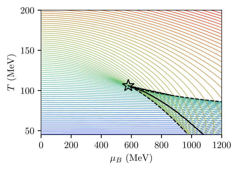
Figure 1: Example of critical point location by finding the point in the $(T,~{}\mu_{B})$ phase diagram where the lines of constant $\phi_{0}$ at increasing $\Phi_{1}$ cross for the first time.

The partially gray lines in the leftmost and middle panels of Fig. 2 display the prior equations of state (entropy density and second order baryon susceptibility $\chi_{2}^{B}$), resulting from the functions $f(\phi)$ and $V(\phi)$ utilized to start the DE-MCMC algorithm. The rightmost panels show the spatial distribution of critical points in the $(T,~{}\mu_{B})$ plane corresponding to these samples of the priors. The top and bottom panels correspond to the PHA and PA models, respectively. It is evident that priors for the PA version of the EMD model cover a wider range for the equation of state, especially for $\chi_{2}^{B}$. While $\sim 20\%$ of the prior sample does not produce a critical point at all for the PA model, critical points found in this sample are scattered over a very wide region in the phase diagram. On the other hand, the prior for the PHA version of the model comparatively produces critical points that are concentrated mainly in one region of the phase diagram.

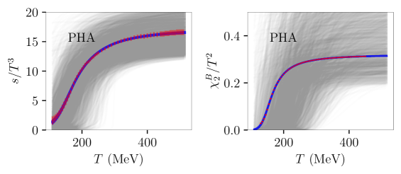
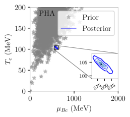
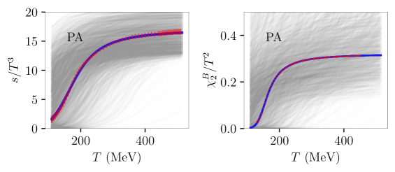
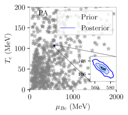
Figure 2: Results for sample equations of state from the prior (gray) and posterior (blue) distributions, for the PHA (top) and PA (bottom) Ansätze. Left: Entropy density, normalized by temperature cubed, as a function of temperature. Center: Second order baryon number susceptibility normalized by temperature squared, as a function of temperature. Right: Predictions for the QCD critical point for the prior (grey stars) and posterior samples (blue histogram and contours). In the left and center panels, the red points with error bars are the lattice results from Refs. Borsanyi:2013bia ; Bellwied:2015lba . In the rightmost panels, the blue lines visible in the inset represent 68% and 95% confidence levels for the posterior distribution.

The DE-MCMC algorithm mentioned above allows us to constrain the model parameters in Eqs. (2)-(5) to reproduce the lattice QCD results for entropy density and second-order baryon number susceptibility, thus yielding samples of the posterior distributions for these functions. Posterior samples for the zero-doping equation of state are shown as blue lines in Fig. 2, together with the lattice QCD results from Refs. Borsanyi:2013bia ; Bellwied:2015lba (red points). Even though, like the prior ones, these samples are shown individually as partially transparent lines, they concentrate in a clear-cut thin blue band, which roughly spans the entire region allowed by the lattice error bars.

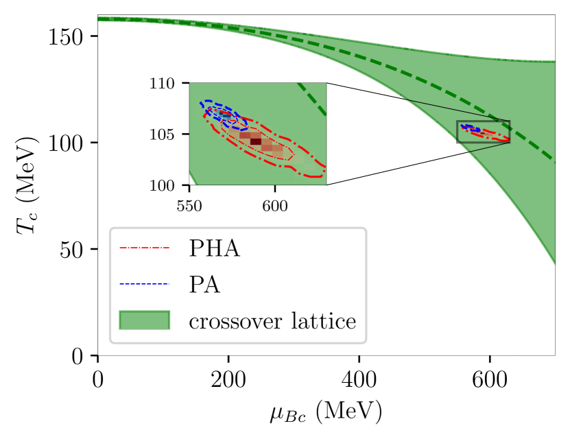
Figure 3: Predictions for the location of the critical point on the $(T,~{}\mu_{B})$-plane, based on the posterior distributions for the PHA model (red area) and the PA model (blue area). Also shown is the extrapolation of the lattice QCD transition line from Ref. Borsanyi:2020fev (green band), based on the peak of the chiral susceptibility. Lines around confidence regions for the critical point location represent $68\%$ and $95\%$ confidence levels.

Figure 3 shows the predicted distributions for the critical point location from our Bayesian analysis for the PHA (red) and PA (blue) Ansätze, together with the corresponding $68\%$ and $95\%$ confidence levels. Differently from what was found for the prior samples, each critical point predicted within the posterior samples is located within a narrow region in $T$ and $\mu_{B}$. Moreover, the regions for the PA and PHA Ansätze agree with each other, with overlapping $68\%$ confidence regions. This indicates that it is the lattice QCD results at zero baryon density that provide the main influence on the location of the critical point in the holographic model, regardless of the functional forms of the model potentials.

Also shown in Fig. 3 is the extrapolation of the lattice QCD crossover line from Ref. Borsanyi:2020fev , based on the peak of the chiral susceptibility (green band). It is evident that both $95\%$ confidence levels for the critical point are contained within the lattice extrapolation band. Since this did not have to be the case, we take this as a strong indication of the predictive power of the lattice QCD results, which strongly constrain the posterior distributions of critical points of the holographic model to a meaningful region of the phase diagram. To enable the comparison to prior critical points, critical points drawn from the posterior are also shown in the insets on the rightmost panels of Fig. 2.

Marginalizing the distribution in Fig. 3 yields the following $95\%$ confidence intervals for the critical temperature $T_{c}$ and chemical potential $\mu_{c}$ :

$$(T_{c},\,\mu_{Bc})_{PHA} = (104\pm 3,\,589^{+36}_{-26})~{}\mathrm{MeV},$$ (6)

$$(T_{c},\,\mu_{Bc})_{PA} = (107\pm 1,\,571\pm 11)~{}\mathrm{MeV}.$$ (7)

These results are compatible with those obtained in Ref. Cai:2022omk .

Next, we provide an estimate for the center-of-mass energy, $\sqrt{s}$, in relativistic heavy-ion collisions that can potentially probe our holographic prediction for the location of the critical point. The analysis of mean hadron multiplicities within transport and statistical hadronization models provides the dependence of the variables $(T,~{}\mu_{B})$ on $\sqrt{s}$ at the point where inelastic collisions cease to promote chemical equilibrium, i.e. the chemical freeze-out point Cleymans:2005xv ; Andronic:2008gu ; Vovchenko:2015idt ; Alba:2020jir . Additionally, the dependence on $\sqrt{s}$ can also be extracted from the measurement of moments of net-particle distributions that can be directly compared with ratios of susceptibilities Alba:2014eba . Taking into account the uncertainties in the location of the critical point from our analysis, we predict a range for the center of mass energy of $\sqrt{s}=4.4\pm 0.4$ GeV for the PHA model, and $\sqrt{s}=4.6^{+0.2}_{-0.1}$ GeV for the PA model (see Fig. 4). These results were obtained by using the statistical hadronization model from Ref. Vovchenko:2015idt for $\mu_{B}(\sqrt{s})$. Predictions for a holographic critical point have been previously presented in Critelli:2017oub ; Li:2023mpv .

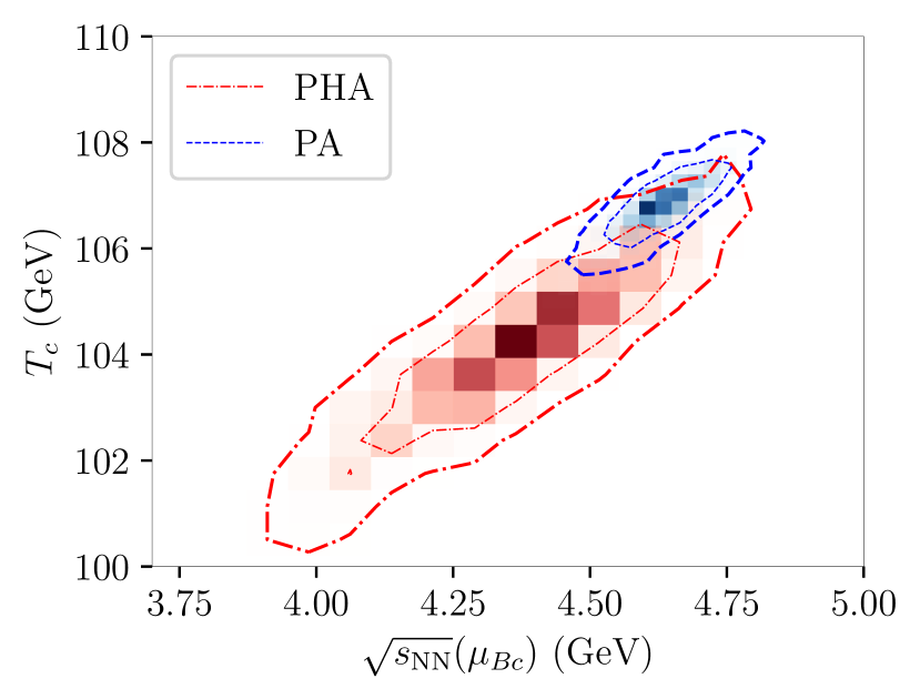
Figure 4: Collision energy dependence of the baryon chemical potential for the critical point from the PA model (Blue, dashed lines) and the PHA model (red, dash-dotted lines). The predicted range for the center of mass energy is $\sqrt{s}=4.4\pm 0.4$ GeV for the PHA model and $\sqrt{s}=4.6^{+0.2}_{-0.1}$ GeV for the PA one. The parametrization for $\mu_{B}(\sqrt{s})$ is taken from Ref. Vovchenko:2015idt . Lines represent $68\%$ and $95\%$ confidence levels.

Conclusions. In this manuscript, we presented the first prediction on the location of the critical point in the high-density phase of strongly interacting matter, obtained through a Bayesian analysis constrained by first principle results at zero density. The analysis has been performed within the Holographic EMD model. Different functional forms for the dilaton field potential and its coupling to the Maxwell field have been tested and constrained to reproduce the lattice QCD results for the entropy density and second-order baryon number susceptibility at $\mu_{B}=0$. While the prior distributions for all functional forms yield critical points that cover wide regions of the phase diagram, or no critical point at all, all posterior predictions for the critical point location collapse around $(T_{c},\,\mu_{Bc})_{PHA}=(104\pm 3,\,589^{+36}_{-26})$ MeV and $(T_{c},\,\mu_{Bc})_{PA}=(107\pm 1,\,571\pm 11)$ MeV. The two regions agree within 1 standard deviation, showing the ability of the lattice results at zero baryon density to strongly constrain the critical point location within the holographic model. We predict that the collision energy needed to discover the critical point lies in the range: $\sqrt{s}=4.0-4.8$ GeV , which is covered by the STAR Fixed Target program and could be explored at FAIR.

Acknowledgements. We thank R. Haas for discussions on computational aspects of this work. We also thank D. Phillips for his insight on how to treat unknown error correlations and theory error, N. Yunes for advice on Bayesian analyses, and D. Mroczek and G. Nijs for fruitful discussions. This material is based upon work supported by the National Science Foundation under grants No. PHY-2208724 and No. PHY-2116686 and in part by the U.S. Department of Energy, Office of Science, Office of Nuclear Physics, under Award Number DE-SC0022023, DE-SC0023861. This work was supported in part by the National Science Foundation (NSF) within the framework of the MUSES collaboration, under grant number No. OAC-2103680. This research was supported in part by the National Science Foundation under Grant No. PHY-1748958.

Here, we provide a more detailed account of the analysis presented in the main text. We discuss our choice of prior distribution, our likelihood function, and our MCMC implementation. We also show more complete results for the posterior distribution and compare predictions from our maximum a posteriori parameters to lattice QCD results at zero and finite baryon density.

I Prior distributions

We have taken prior distributions to be uniform over most parameters, within the ranges shown in Table 1. The sole exceptions are the parameters $d_{2}$, in the PHA model, and $\delta\phi_{1}$, in the PA model, for which we employ Jeffreys prior distributions (uniform over the logarithm of these parameters), also within the ranges indicated in Table 1, where they are marked by a ‘(J)’. Prior ranges for the parameters in $V(\phi)$ are chosen keeping in mind that $V(\phi)$ should have a single maximum at $\phi=0$ and so that $-4\leq V^{\prime\prime}(0)<0$.

An extra parameter in the likelihood function is given by the correlation between neighboring points $0\leq\Gamma<1$. Accordingly, we take the prior for this parameter in the interval $[0,1)$.

As a starting point for the Markov Chain Monte Carlo, priors are initially sampled in a Latin hypercube configuration using library pyDOE, with 500 points per parameter for the PHA model, and 200 points per parameter for the PA model.

PHA Ansatz
Parameter	min	max
$\Lambda$	800 MeV	1400 MeV
$\kappa_{2}$	9.0	15.0
$\gamma$	0.5682	0.6500
$b_{2}$	-0.05	0.65
$b_{4}$	-0.150	-0.015
$b_{6}$	-0.00200	0.00169
$c_{1}$	-0.035	0.100
$c_{2}$	0.1	1.5
$c_{3}$	0.0	1.0
$d_{1}$	0.0	2.5
(J) $d_{2}$ (J)	3	10000

PA Ansatz
Parameter	min	max
$\Lambda$	400 MeV	1400 MeV
$\kappa_{2}$	9.0	15.0
$\gamma_{1}$	0.40	0.57
$\gamma_{2}$	0.50	0.68
$\Delta\phi_{V}$	1.5	3.0
$A$	0.25	0.50
$\phi_{1}$	-0.1	0.5
(J) $\delta\phi_{1}$ (J)	$10^{-5}$	0.3
$\phi_{2}$	0.8	4.5
$\delta\phi_{2}$	0.2	4.0

Table 1: Prior ranges for parameters in the PHA (left) and PA (right) models. The ‘(J)’ marks parameters for which we have used Jeffreys priors — i.e., prior distributions that are uniform over the logarithm of these parameters.

PHA	Posterior 95% CI
Parameter	min	max	MAP
$\Lambda$	1089 MeV	1190 MeV	1129 MeV
$\kappa_{2}$	11.3	11.5	11.4
$\gamma$	0.57	0.63	0.58
$b_{2}$	0.1	0.5	0.2
$b_{4}$	-0.06	-0.03	-0.05
$b_{6}$	0.000	0.002	0.0007
$c_{1}$	-0.1	0.1	0.0
$c_{2}$	0.1	0.3	0.2
$c_{3}$	0.01	0.08	0.04
$d_{1}$	1.70	1.74	1.72
(J) $d_{2}$ (J)	113	8068	1294

PA	Posterior 95% CI
Parameter	min	max	MAP
$\Lambda$	862 MeV	1043 MeV	955 MeV
$\kappa_{2}$	11.3	11.5	11.4
$\gamma_{1}$	0.50	0.54	0.52
$\gamma_{2}$	0.60	0.62	0.61
$\Delta\phi_{V}$	1.6	2.1	1.8
$A$	0.369	0.374	0.371
$\phi_{1}$	0.000	0.025	0.002
(J) $\delta\phi_{1}$ (J)	0.0001	0.0032	0.0003
$\phi_{2}$	2.1	2.3	2.2
$\delta\phi_{2}$	0.65	0.73	0.69

Table 2: Posterior 95% confidence intervals (95% CI) and maximum a posteriori (MAP) values for parameters of the PHA (left) and PA (right) models. The ‘(J)’ marks parameters for which we have used Jeffreys priors — i.e., prior distributions that are uniform over the logarithm of these parameters. MAP values are extracted by maximizing the likelihood.

II Likelihood function

The agreement between predictions $\vec{p}(\theta)$ of the model with parameters $\theta$ and lattice QCD results $\vec{d}$ is quantified by the likelihood function $\mathcal{L}(\vec{\theta})\equiv P(\vec{d}|\vec{\theta})$.

We take a Gaussian likelihood

$$\mathcal{L}(\vec{\theta})=\frac{1}{\,\displaystyle\prod_{Q=s,\chi_{2}}\left[\left(\prod_{i}\sigma_{i}^{(Q)}\right)\sqrt{2\pi\det{\Lambda}}\right]}\exp\left\{-\frac{1}{2}\sum_{i,j}\sum_{Q=s,\chi_{2}}\frac{p_{i}^{(Q)}(\vec{\theta})-d_{i}^{(Q)}}{\sigma_{i}^{(Q)}}\left[\Lambda^{-1}\right]_{ij}\frac{p_{j}^{(Q)}(\vec{\theta})-d_{j}^{(Q)}}{\sigma_{j}^{(Q)}}\right\},$$ (S.1)

where $\sigma_{i}^{(Q)}$, with $Q=s,\chi_{2}^{B}$ represent error bars for the different points from lattice QCD.

The matrix $\Lambda$ is responsible for implementing correlations between neighboring points, by introducing an extra parameter $\Gamma=0-1$:

$$\Lambda_{ij}=\Gamma^{-|T_{i}-T_{j}|/\Delta T},$$ (S.2)

where $\Delta T$ is the temperature step used to match all the points from lattice QCD. In principle, the determinant of $\Lambda$ should be computed only over the points where lattice results exist, since points are not always equally spaced and in the same interval for the two quantities in question. In practice, however, for simplicity, we assume there are $N=(T_{\textrm{max}}-T_{\textrm{min}})/\Delta T+1$ and take

$$\det\Lambda\approx(1-\Gamma^{2})^{N-1}.$$ (S.3)

Finally, the logarithm of the likelihood becomes sivia1996data

$$\log\mathcal{L}=\frac{-1}{1-\Gamma^{2}}\left[(1+\Gamma^{2})\,\zeta^{2}-\Gamma\,\psi-\Gamma^{2}\,\phi\right]-(N-1)\,\log(1-\Gamma^{2})+\text{const.}\,,$$ (S.4)

where

$$\zeta^{2} \equiv\frac{1}{2}\sum_{i}\sum_{Q=s,\chi_{2}}\left(\frac{p_{i}^{(Q)}(\vec{\theta})-d_{i}^{(Q)}}{\sigma_{i}^{(Q)}}\right)^{2},$$ (S.5)

$$\psi \equiv\sum_{i}\sum_{Q=s,\chi_{2}}\frac{p_{i}^{(Q)}(\vec{\theta})-d_{i}^{(Q)}}{\sigma_{i}^{(Q)}}\frac{p_{i+1}^{(Q)}(\vec{\theta})-d_{i+1}^{(Q)}}{\sigma_{i+1}^{(Q)}},$$ (S.6)

$$\phi \equiv\frac{1}{2}\left[\left(\frac{p_{1}^{(Q)}(\vec{\theta})-d_{1}^{(Q)}}{\sigma_{1}^{(Q)}}\right)^{2}+\left(\frac{p_{N}^{(Q)}(\vec{\theta})-d_{N}^{(Q)}}{\sigma_{N}^{(Q)}}\right)^{2}\right].$$ (S.7)

Remarkably, the posterior $95\%$ confidence interval obtained for the correlation strength is of $\Gamma=0.84^{+0.03}_{-0.06}$, for both the PHA and PA models. This impressive agreement indicates that its value does not reflect the parametrization, but rather the lattice QCD error bars.

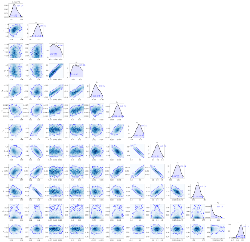
Figure 5: Marginalized a posteriori probability distributions for pairs of parameters of the PHA model. Solid lines show 95% confidence intervals. On the diagonal, marginalized one-parameter posterior distributions are also shown, along with the marginalized maximum a posteriori (MMAP) value and 95% confidence interval for each parameter. MMAP values are extracted by maximizing the marginalized one-parameter posterior distributions.

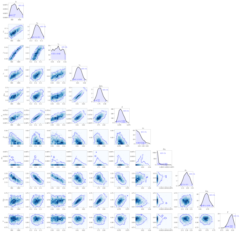
Figure 6: Marginalized a posteriori probability distributions for pairs of parameters of the PA model. Solid lines show 95% confidence intervals. On the diagonal, marginalized one-parameter posterior distributions are also shown, along with the marginalized maximum a posteriori (MMAP) value and 95% confidence interval for each parameter. MMAP values are extracted by maximizing the marginalized one-parameter posterior distributions.

III DE-MCMC Algorithm

To carry out our analyses, we had to overcome numerical challenges for the convergence of the MCMC. First of all, parameters in our posterior distributions turn out to be highly correlated. Furthermore, due to the small errors in lattice results, especially for the second-order baryon susceptibility, our posterior is strongly dominated by the likelihood, which delays the convergence of the MCMC.

To overcome numerical challenges posed by correlations in a simple manner, we employ differential evolution MCMC (DE-MCMC) speagle2019conceptual,2006S&C….16..239T, with a simple Metropolis acceptance criterion. To avoid issues with local maxima of the posterior function, we employ the common strategy of increasing the relative step size every 10 iterations, so that each Monte Carlo chain can hop between local maxima 2006S&C….16..239T. To ensure all the chains reflect the same probability distribution so that DE-MCMC works in ideal conditions, enhancing the convergence of the algorithm, we also employ a simple sequential tempering of all the chains, choosing random starting samples from the previous step, according to the update in temperature, every time the MCMC temperature changes. After the MCMC temperature reaches $1$, we let each chain evolve without interference.

IV Posterior distributions

After convergence is found, we collect samples. To ensure statistical independence between samples, we “thin out” the data (i.e., skip samples) according to the measured correlation time.

The resulting posterior distributions for the parameters of the PHA and PA models are illustrated in the corner plots in Figs. 5 and 6, respectively, where 95% confidence levels are also shown.

The same 95% confidence intervals are shown in Table 2. However, in that table, maximum a posteriori parameters are extracted from the point of maximum likelihood, while in Figs. 5 and 6, marginalized maximum a posteriori parameters are extracted from the marginalized distribution for each parameter.

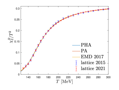
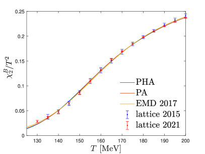
Figure 7: Second order baryon susceptibility $\chi_{2}^{B}$ at zero chemical potential from the best fit to lattice data from Ref. Borsanyi:2021sxv for PHA and PA. For comparison, we also show the previous lattice result for this susceptibility from Ref. Bellwied:2015lba and the resulting fitting for our previous EMD model from Refs. Critelli:2017oub,Grefa:2021qvt

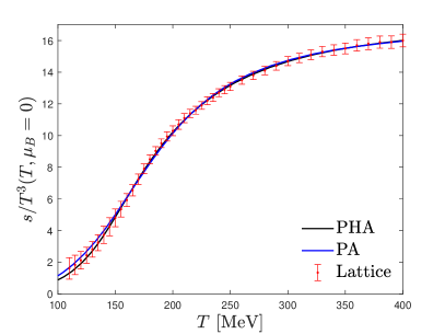
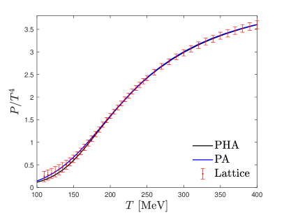
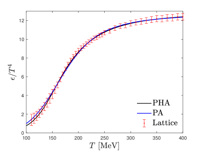
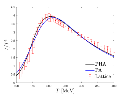
Figure 8: Comparison between the best fit for the PHA and PA models and the lattice equation of state at zero chemical potential from Ref. Borsanyi:2013bia

V Comparison with lattice QCD results

In this section, we compare state-of-the-art lattice QCD results to the corresponding holographic postdictions for the PA and PHA models, with the best-fit parameters from the Bayesian analysis. In Fig. 7 we present the comparison of the second-order baryon susceptibility at $\mu_{B}=0$ between the holographic model and the Lattice QCD results from Ref. Borsanyi:2021sxv, which were used to constrain the PA and PHA models. For further contrast, we also show the previous lattice data from Ref. Bellwied:2015lba and the previous holographic result from Refs. Critelli:2017oub,Grefa:2021qvt. It is worth noticing that the error bars for the lattice susceptibility have reduced, and the holographic susceptibility from both models almost overlaps completely.

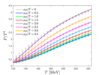
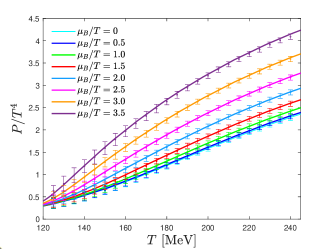
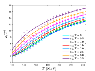
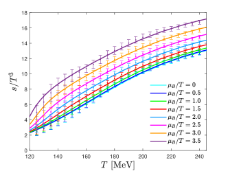
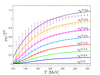
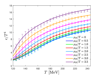
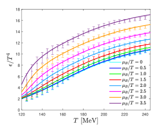
Figure 9: Comparison between the Equation of State at finite density obtained from the best fit to lattice data at zero chemical potential for the PHA model (left) and the PA one (right), and the state-of-the-art lattice QCD results from Borsanyi:2021sxv.

In Fig. 8, we also show the holographic results in the PA and PHA models for the equation of state at zero chemical potential, compared to the lattice results from Borsanyi:2013bia. It is important to remark that the entropy density, together with the second-order baryon susceptibility, is the quantity that is matched to the lattice result, whereas other thermodynamic quantities are computed directly from thermodynamic identities.

One can observe minor differences between the best PHA and PA models. The PA model gets closer to the lattice data at very low T, but then the PHA model gets a better agreement after the third lowest temperature point, although both are within error bars. At some point, both results completely overlap in the case of the entropy density and pressure. However, for the trace anomaly, the PHA model is in better agreement with the corresponding lattice results. This is not too surprising, since the lattice error bars are large at low $T$, which means that those data points are the least constrained in the Bayesian analysis. Thus, the models with the highest likelihood are the ones that fit the high $T$ error bars, which are much smaller. At high temperatures, the results from both PA and PHA completely overlap.

However, the most important comparison is the one between the predicted holographic equation of state and the most recent lattice results for the QCD equation of state at finite temperature and chemical potential. This comparison with the lattice results from Ref. Borsanyi:2021sxv is shown in Fig. 9. One can note that the holographic prediction for the entropy density in the PHA (left) and PA (right) models are in numerical agreement with the lattice points, although, in the case of the pressure and energy density, the holographic results start to deviate from the lattice prediction when $\mu_{B}/T\geq 3.5$. Similarly to what was reported in our previous work Grefa:2021qvt , the holographic baryon density is in agreement with the lattice results up to $T\approx 190$ MeV for all values of $\mu_{B}/T$. Additionally, one difference we observe is the location of the critical point from the best fit (i.e, maximum likelihood parameters) for each model. The predicted critical point for the PHA model with the highest likelihood is found at $T_{c}=103.45$ MeV, and $\mu_{Bc}=599$ MeV, whereas for the PA case, the critical point is located at $T_{c}=106.72$ MeV, $\mu_{Bc}=573$ MeV.

unsrturl reference,noninspire

References

- (1) Y. Aoki, G. Endrodi, Z. Fodor, S. D. Katz, and K. K. Szabo. The Order of the quantum chromodynamics transition predicted by the standard model of particle physics. Nature, 443:675–678, 2006. arXiv:hep-lat/0611014, doi:10.1038/nature05120.
- (2) Steven Weinberg. Cosmology. 2008.
- (3) Ulrich Heinz and Raimond Snellings. Collective flow and viscosity in relativistic heavy-ion collisions. Ann. Rev. Nucl. Part. Sci., 63:123–151, 2013. arXiv:1301.2826, doi:10.1146/annurev-nucl-102212-170540.
- (4) Miklos Gyulassy and Larry McLerran. New forms of QCD matter discovered at RHIC. Nucl. Phys. A, 750:30–63, 2005. arXiv:nucl-th/0405013, doi:10.1016/j.nuclphysa.2004.10.034.
- (5) Edward V. Shuryak. What RHIC experiments and theory tell us about properties of quark-gluon plasma? Nucl. Phys. A, 750:64–83, 2005. arXiv:hep-ph/0405066, doi:10.1016/j.nuclphysa.2004.10.022.
- (6) Matthias Troyer and Uwe-Jens Wiese. Computational complexity and fundamental limitations to fermionic quantum Monte Carlo simulations. Phys. Rev. Lett., 94:170201, 2005. arXiv:cond-mat/0408370, doi:10.1103/PhysRevLett.94.170201.
- (7) Misha A. Stephanov, K. Rajagopal, and Edward V. Shuryak. Signatures of the tricritical point in QCD. Phys. Rev. Lett., 81:4816–4819, 1998. arXiv:hep-ph/9806219, doi:10.1103/PhysRevLett.81.4816.
- (8) Veronica Dexheimer, Jorge Noronha, Jacquelyn Noronha-Hostler, Claudia Ratti, and Nicolás Yunes. Future physics perspectives on the equation of state from heavy ion collisions to neutron stars. J. Phys. G, 48(7):073001, 2021. arXiv:2010.08834, doi:10.1088/1361-6471/abe104.
- (9) D. Almaalol et al. QCD Phase Structure and Interactions at High Baryon Density: Continuation of BES Physics Program with CBM at FAIR. 9 2022. arXiv:2209.05009.
- (10) Alessandro Lovato et al. Long Range Plan: Dense matter theory for heavy-ion collisions and neutron stars. 11 2022. arXiv:2211.02224.
- (11) Agnieszka Sorensen et al. Dense Nuclear Matter Equation of State from Heavy-Ion Collisions. 1 2023. arXiv:2301.13253.
- (12) Rajesh Kumar et al. Theoretical and Experimental Constraints for the Equation of State of Dense and Hot Matter. 3 2023. arXiv:2303.17021.
- (13) Juan Martin Maldacena. The Large N limit of superconformal field theories and supergravity. Adv. Theor. Math. Phys., 2:231–252, 1998. arXiv:hep-th/9711200, doi:10.4310/ATMP.1998.v2.n2.a1.
- (14) S. S. Gubser, Igor R. Klebanov, and Alexander M. Polyakov. Gauge theory correlators from noncritical string theory. Phys. Lett. B, 428:105–114, 1998. arXiv:hep-th/9802109, doi:10.1016/S0370-2693(98)00377-3.
- (15) Edward Witten. Anti-de Sitter space and holography. Adv. Theor. Math. Phys., 2:253–291, 1998. arXiv:hep-th/9802150, doi:10.4310/ATMP.1998.v2.n2.a2.
- (16) Edward Witten. Anti-de Sitter space, thermal phase transition, and confinement in gauge theories. Adv. Theor. Math. Phys., 2:505–532, 1998. arXiv:hep-th/9803131, doi:10.4310/ATMP.1998.v2.n3.a3.
- (17) Dam T. Son and Andrei O. Starinets. Viscosity, Black Holes, and Quantum Field Theory. Ann. Rev. Nucl. Part. Sci., 57:95–118, 2007. arXiv:0704.0240, doi:10.1146/annurev.nucl.57.090506.123120.
- (18) Steven S. Gubser and Andreas Karch. From gauge-string duality to strong interactions: A Pedestrian’s Guide. Ann. Rev. Nucl. Part. Sci., 59:145–168, 2009. arXiv:0901.0935, doi:10.1146/annurev.nucl.010909.083602.
- (19) P. Kovtun, Dan T. Son, and Andrei O. Starinets. Viscosity in strongly interacting quantum field theories from black hole physics. Phys. Rev. Lett., 94:111601, 2005. arXiv:hep-th/0405231, doi:10.1103/PhysRevLett.94.111601.
- (20) Oliver DeWolfe, Steven S. Gubser, and Christopher Rosen. A holographic critical point. Phys. Rev. D, 83:086005, 2011. arXiv:1012.1864, doi:10.1103/PhysRevD.83.086005.
- (21) Renato Critelli, Jorge Noronha, Jacquelyn Noronha-Hostler, Israel Portillo, Claudia Ratti, and Romulo Rougemont. Critical point in the phase diagram of primordial quark-gluon matter from black hole physics. Phys. Rev. D, 96(9):096026, 2017. arXiv:1706.00455, doi:10.1103/PhysRevD.96.096026.
- (22) Romulo Rougemont, Renato Critelli, and Jorge Noronha. Nonhydrodynamic quasinormal modes and equilibration of a baryon dense holographic QGP with a critical point. Phys. Rev. D, 98(3):034028, 2018. arXiv:1804.00189, doi:10.1103/PhysRevD.98.034028.
- (23) Joaquin Grefa, Jorge Noronha, Jacquelyn Noronha-Hostler, Israel Portillo, Claudia Ratti, and Romulo Rougemont. Hot and dense quark-gluon plasma thermodynamics from holographic black holes. Phys. Rev. D, 104(3):034002, 2021. arXiv:2102.12042, doi:10.1103/PhysRevD.104.034002.
- (24) Joaquin Grefa, Mauricio Hippert, Jorge Noronha, Jacquelyn Noronha-Hostler, Israel Portillo, Claudia Ratti, and Romulo Rougemont. Transport coefficients of the quark-gluon plasma at the critical point and across the first-order line. Phys. Rev. D, 106(3):034024, 2022. arXiv:2203.00139, doi:10.1103/PhysRevD.106.034024.
- (25) Szabocls Borsanyi, Zoltan Fodor, Christian Hoelbling, Sandor D. Katz, Stefan Krieg, and Kalman K. Szabo. Full result for the QCD equation of state with 2+1 flavors. Phys. Lett. B, 730:99–104, 2014. arXiv:1309.5258, doi:10.1016/j.physletb.2014.01.007.
- (26) R. Bellwied, S. Borsanyi, Z. Fodor, S. D. Katz, A. Pasztor, C. Ratti, and K. K. Szabo. Fluctuations and correlations in high temperature QCD. Phys. Rev. D, 92(11):114505, 2015. arXiv:1507.04627, doi:10.1103/PhysRevD.92.114505.
- (27) S. Borsányi, Z. Fodor, J. N. Guenther, R. Kara, S. D. Katz, P. Parotto, A. Pásztor, C. Ratti, and K. K. Szabó. Lattice QCD equation of state at finite chemical potential from an alternative expansion scheme. Phys. Rev. Lett., 126(23):232001, 2021. arXiv:2102.06660, doi:10.1103/PhysRevLett.126.232001.
- (28) Romulo Rougemont, Joaquin Grefa, Mauricio Hippert, Jorge Noronha, Jacquelyn Noronha-Hostler, Israel Portillo, and Claudia Ratti. Hot QCD Phase Diagram From Holographic Einstein-Maxwell-Dilaton Models. 7 2023. arXiv:2307.03885.
- (29) Steven S. Gubser and Abhinav Nellore. Mimicking the QCD equation of state with a dual black hole. Phys. Rev. D, 78:086007, 2008. arXiv:0804.0434, doi:10.1103/PhysRevD.78.086007.
- (30) Steven S. Gubser, Abhinav Nellore, Silviu S. Pufu, and Fabio D. Rocha. Thermodynamics and bulk viscosity of approximate black hole duals to finite temperature quantum chromodynamics. Phys. Rev. Lett., 101:131601, 2008. arXiv:0804.1950, doi:10.1103/PhysRevLett.101.131601.
- (31) Oliver DeWolfe, Steven S. Gubser, and Christopher Rosen. Dynamic critical phenomena at a holographic critical point. Phys. Rev. D, 84:126014, 2011. arXiv:1108.2029, doi:10.1103/PhysRevD.84.126014.
- (32) Stefano I. Finazzo, Romulo Rougemont, Hugo Marrochio, and Jorge Noronha. Hydrodynamic transport coefficients for the non-conformal quark-gluon plasma from holography. JHEP, 02:051, 2015. arXiv:1412.2968, doi:10.1007/JHEP02(2015)051.
- (33) Romulo Rougemont, Andrej Ficnar, Stefano Finazzo, and Jorge Noronha. Energy loss, equilibration, and thermodynamics of a baryon rich strongly coupled quark-gluon plasma. JHEP, 04:102, 2016. arXiv:1507.06556, doi:10.1007/JHEP04(2016)102.
- (34) Romulo Rougemont, Jorge Noronha, and Jacquelyn Noronha-Hostler. Suppression of baryon diffusion and transport in a baryon rich strongly coupled quark-gluon plasma. Phys. Rev. Lett., 115(20):202301, 2015. arXiv:1507.06972, doi:10.1103/PhysRevLett.115.202301.
- (35) Stefano Ivo Finazzo and Romulo Rougemont. Thermal photon, dilepton production, and electric charge transport in a baryon rich strongly coupled QGP from holography. Phys. Rev. D, 93(3):034017, 2016. arXiv:1510.03321, doi:10.1103/PhysRevD.93.034017.
- (36) Romulo Rougemont, Renato Critelli, Jacquelyn Noronha-Hostler, Jorge Noronha, and Claudia Ratti. Dynamical versus equilibrium properties of the QCD phase transition: A holographic perspective. Phys. Rev. D, 96(1):014032, 2017. arXiv:1704.05558, doi:10.1103/PhysRevD.96.014032.
- (37) Rong-Gen Cai, Song He, Li Li, and Yuan-Xu Wang. Probing QCD critical point and induced gravitational wave by black hole physics. Phys. Rev. D, 106(12):L121902, 2022. arXiv:2201.02004, doi:10.1103/PhysRevD.106.L121902.
- (38) Zhibin Li, Jingmin Liang, Song He, and Li Li. Holographic study of higher-order baryon number susceptibilities at finite temperature and density. Phys. Rev. D, 108(4):046008, 2023. arXiv:2305.13874, doi:10.1103/PhysRevD.108.046008.
- (39) J. Knaute and B. Kämpfer. Holographic Entanglement Entropy in the QCD Phase Diagram with a Critical Point. Phys. Rev. D, 96(10):106003, 2017. arXiv:1706.02647, doi:10.1103/PhysRevD.96.106003.
- (40) Szabolcs Borsanyi, Zoltan Fodor, Jana N. Guenther, Ruben Kara, Sandor D. Katz, Paolo Parotto, Attila Pasztor, Claudia Ratti, and Kalman K. Szabo. QCD Crossover at Finite Chemical Potential from Lattice Simulations. Phys. Rev. Lett., 125(5):052001, 2020. arXiv:2002.02821, doi:10.1103/PhysRevLett.125.052001.
- (41) J. Cleymans, H. Oeschler, K. Redlich, and S. Wheaton. Comparison of chemical freeze-out criteria in heavy-ion collisions. Phys. Rev. C, 73:034905, 2006. arXiv:hep-ph/0511094, doi:10.1103/PhysRevC.73.034905.
- (42) A. Andronic, P. Braun-Munzinger, and J. Stachel. Thermal hadron production in relativistic nuclear collisions: The Hadron mass spectrum, the horn, and the QCD phase transition. Phys. Lett. B, 673:142–145, 2009. [Erratum: Phys.Lett.B 678, 516 (2009)]. arXiv:0812.1186, doi:10.1016/j.physletb.2009.06.021.
- (43) V. Vovchenko, V. V. Begun, and M. I. Gorenstein. Hadron multiplicities and chemical freeze-out conditions in proton-proton and nucleus-nucleus collisions. Phys. Rev. C, 93(6):064906, 2016. arXiv:1512.08025, doi:10.1103/PhysRevC.93.064906.
- (44) P. Alba, V. Mantovani Sarti, J. Noronha-Hostler, P. Parotto, I. Portillo-Vazquez, C. Ratti, and J. M. Stafford. Influence of hadronic resonances on the chemical freeze-out in heavy-ion collisions. Phys. Rev. C, 101(5):054905, 2020. arXiv:2002.12395, doi:10.1103/PhysRevC.101.054905.
- (45) Paolo Alba, Wanda Alberico, Rene Bellwied, Marcus Bluhm, Valentina Mantovani Sarti, Marlene Nahrgang, and Claudia Ratti. Freeze-out conditions from net-proton and net-charge fluctuations at RHIC. Phys. Lett. B, 738:305–310, 2014. arXiv:1403.4903, doi:10.1016/j.physletb.2014.09.052.
Supplemental Material